an interactive tool for teaching transmission line
TRANSCRIPT

An Interactive Tool for Teaching Transmission Line Concepts
by
Keaton Scheible
A THESIS
submitted to
Oregon State University
Honors College
in partial fulfillment of
the requirements for the
degree of
Honors Baccalaureate of Science in Electrical and Computer Engineering
(Honors Associate)
Presented June 1, 2017
Commencement June 2017


AN ABSTRACT OF THE THESIS OF
Keaton Scheible for the degree of Honors Baccalaureate of Science in Electrical and
Computer Engineering presented on June 1, 2017. Title: An Interactive Tool for Teaching
Transmission Line Concepts.
Abstract approved:_____________________________________________________
Andreas Weisshaar
In college transmission lines courses, students are expected to understand how different
circuit configurations affect the signals on a transmission line. Having a way to visualize
these signals can greatly improve their learning experience. This thesis details the
development of an open source, interactive learning tool used to illustrate fundamental
transmission line concepts. The tool provides an engaging environment that lets students
construct circuits and generate transient and steady state animations for lossless and lossy
lines, respectively. A variety of adjustable sources and loads are available, letting students
explore a range of transmission line phenomena. Matlab was chosen for the development
of this tool, and all source code is freely available online. The hope is that students and
educators will learn from this tool and develop it further to create additional avenues for
understanding transmission line concepts.
Key Words: transmission line, open source, electrical, engineering, Matlab, interactive
Corresponding e-mail address: [email protected]

©Copyright by Keaton Scheible
June 1, 2017
All Rights Reserved

An Interactive Tool for Teaching Transmission Line Concepts
by
Keaton Scheible
A THESIS
submitted to
Oregon State University
Honors College
in partial fulfillment of
the requirements for the
degree of
Honors Baccalaureate of Science in Electrical and Computer Engineering
(Honors Associate)
Presented June 1, 2017
Commencement June 2017

Honors Baccalaureate of Science in Electrical and Computer Engineering project of
Keaton Scheible presented on June 1, 2017.
APPROVED:
_____________________________________________________________________
Andreas Weisshaar, Mentor, representing Electrical and Computer Engineering
_____________________________________________________________________
Albrecht Jander, Committee Member, representing Electrical and Computer Engineering
_____________________________________________________________________
Lei Zheng, Committee Member, representing Electrical and Computer Engineering
_____________________________________________________________________
Toni Doolen, Dean, Oregon State University Honors College
I understand that my project will become part of the permanent collection of Oregon
State University, Honors College. My signature below authorizes release of my project
to any reader upon request.
_____________________________________________________________________
Keaton Scheible, Author
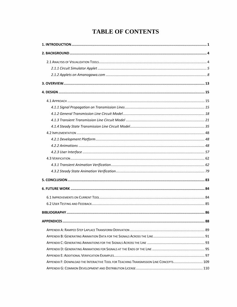
TABLE OF CONTENTS
1. INTRODUCTION ...................................................................................................................................... 1
2. BACKGROUND ........................................................................................................................................ 4
2.1 ANALYSIS OF VISUALIZATION TOOLS........................................................................................................... 4
2.1.1 Circuit Simulator Applet ............................................................................................................ 5
2.1.2 Applets on Amanogawa.com .................................................................................................... 8
3. OVERVIEW............................................................................................................................................ 13
4. DESIGN ................................................................................................................................................. 15
4.1 APPROACH ........................................................................................................................................ 15
4.1.1 Signal Propagation on Transmission Lines ............................................................................... 15
4.1.2 General Transmission Line Circuit Model ................................................................................. 18
4.1.3 Transient Transmission Line Circuit Model .............................................................................. 21
4.1.4 Steady State Transmission Line Circuit Model.......................................................................... 35
4.2 IMPLEMENTATION ............................................................................................................................... 48
4.2.1 Development Platform ............................................................................................................ 48
4.2.2 Animations ............................................................................................................................. 48
4.2.3 User Interface ......................................................................................................................... 57
4.3 VERIFICATION ..................................................................................................................................... 62
4.3.1 Transient Animation Verification ............................................................................................. 62
4.3.2 Steady State Animation Verification ........................................................................................ 79
5. CONCLUSION ........................................................................................................................................ 83
6. FUTURE WORK ..................................................................................................................................... 84
6.1 IMPROVEMENTS ON CURRENT TOOL ........................................................................................................ 84
6.2 USER TESTING AND FEEDBACK ................................................................................................................ 85
BIBLIOGRAPHY ......................................................................................................................................... 86
APPENDICES ............................................................................................................................................. 88
APPENDIX A: RAMPED STEP LAPLACE TRANSFORM DERIVATION .......................................................................... 89
APPENDIX B: GENERATING ANIMATION DATA FOR THE SIGNALS ACROSS THE LINE ................................................... 91
APPENDIX C: GENERATING ANIMATIONS FOR THE SIGNALS ACROSS THE LINE ......................................................... 93
APPENDIX D: GENERATING ANIMATIONS FOR SIGNALS AT THE ENDS OF THE LINE .................................................... 95
APPENDIX E: ADDITIONAL VERIFICATION EXAMPLES .......................................................................................... 97
APPENDIX F: DOWNLOAD THE INTERACTIVE TOOL FOR TEACHING TRANSMISSION LINE CONCEPTS ............................. 109
APPENDIX G: COMMON DEVELOPMENT AND DISTRIBUTION LICENSE .................................................................. 110

LIST OF FIGURES
Figure 1: Standing Waves Pattern....................................................................................... 2
Figure 2: Lattice Diagram ................................................................................................... 2
Figure 3: Signal Propagation on a Transmission Line [3] .................................................. 5
Figure 4: Standing Wave on a Transmission Line [4] ........................................................ 6
Figure 5: Reflections Caused by Transmission Line Terminations [5] .............................. 6
Figure 6: Interactive Smith Chart General Lossy Line [6] ................................................. 8
Figure 7: Interactive Smith Chart General Lossy Line Plots [6] ........................................ 9
Figure 8: General Lossy Line (wide plots) [7].................................................................. 10
Figure 9: General Lossy Line (wide plots) Plot [7] .......................................................... 10
Figure 10: Transient Line with Capacitive Load [8] ........................................................ 11
Figure 11: Transmission Line Circuit and Lattice Diagram ............................................. 16
Figure 12: Step Source ...................................................................................................... 18
Figure 13: Ramped Step Source ....................................................................................... 19
Figure 14: Transient Sinusoidal Source ............................................................................ 19
Figure 15: Supported Loads .............................................................................................. 20
Figure 16: Transmission Line Circuit and s-Domain Lattice Diagram ............................ 26
Figure 17: Lossy Transmission Line Circuit and Lattice Diagram ................................... 38
Figure 18: Forward Traveling Voltage Wave for Transient Animation ........................... 53
Figure 19: Backward Traveling Voltage Wave for Transient Animation ........................ 54
Figure 20: Editable Circuit Diagram for a Lossless Transmission Line ........................... 57
Figure 21: Editable Circuit Diagram for a Lossy Transmission Line ............................... 57
Figure 22: Source Selection Screen .................................................................................. 58
Figure 23: Load Selection Screen ..................................................................................... 58
Figure 24: Animation Settings Screen .............................................................................. 59
Figure 25: Transient Animation ........................................................................................ 60
Figure 26: Steady State Animation ................................................................................... 61
Figure 27: Transient Animation Verification – Step Circuit (Tool) ................................. 63
Figure 28: Transient Animation Verification – Step Circuit (LTspice) ........................... 63

Figure 29: Transient Animation Verification – Step Circuit (Plots) ................................. 64
Figure 33: Transient Animation Verification – Ramped Step Circuit (Tool) ................... 65
Figure 34: Transient Animation Verification – Ramped Step Circuit (LTspice) ............. 65
Figure 35: Transient Animation Verification – Ramped Step Circuit (Plots) .................. 66
Figure 39: Transient Animation Verification – Sine Circuit (Tool) ................................. 67
Figure 40: Transient Animation Verification – Sine Circuit (LTspice) ........................... 67
Figure 41: Transient Animation Verification – Sine Circuit (Plots) ................................. 68
Figure 45: Transient Animations Approaching Steady State – Step Circuit .................... 70
Figure 46: Transient Voltage Approaching Steady State – Step Circuit .......................... 71
Figure 47: Transient Current Approaching Steady State – Step Circuit ........................... 72
Figure 48: Transient Animations Approaching Steady State – Ramped Step Circuit ...... 73
Figure 49: Transient Voltage Approaching Steady State – Ramped Step Circuit ............ 74
Figure 50: Transient Current Approaching Steady State – Ramped Step Circuit ............ 75
Figure 51: Transient Animations Approaching Steady State – Sine Circuit .................... 76
Figure 52: Transient Voltage Approaching Steady State – Sine Circuit .......................... 77
Figure 53: Transient Current Approaching Steady State – Sine Circuit ........................... 78
Figure 54: Steady State Verification – Circuit 1 (Tool) ................................................... 80
Figure 55: Steady State Verification – Circuit 1 (Online) [7] .......................................... 80
Figure 56: Steady State Standing Wave Patterns Created by Tool – Circuit 1................. 81
Figure 57: Steady State Standing Wave Patterns Created by Online (A) – Circuit 1 [7] . 81
Figure 58: Steady State Standing Wave Patterns Created by Online (B) – Circuit 1 [7] . 82
Figure 69: Creating the Ramped Step Function ................................................................ 89
Figure 30: Transient Animation Verification – Step Circuit 2 (Tool) .............................. 97
Figure 31: Transient Animation Verification – Step Circuit 2 (LTspice) ........................ 97
Figure 32: Transient Animation Verification – Step Circuit 2 (Plots) .............................. 98
Figure 36: Transient Animation Verification – Ramped Step Circuit 2 (Tool) ................ 99
Figure 37: Transient Animation Verification – Ramped Step Circuit 2 (LTspice) .......... 99
Figure 38: Transient Animation Verification – Ramped Step Circuit 2 (Plots) ............. 100
Figure 42: Transient Animation Verification – Sine Circuit 2 (Tool) ............................ 101
Figure 43: Transient Animation Verification – Sine Circuit 2 (LTspice) ...................... 101

Figure 44: Transient Animation Verification – Sine Circuit 2 (Plots) ............................ 102
Figure 59: Steady State Verification – Circuit 2 (Tool) ................................................. 103
Figure 60: Steady State Verification – Circuit 2 (Online) [7] ........................................ 103
Figure 61: Steady State Standing Wave Patterns Created by Tool – Circuit 2............... 104
Figure 62: Steady State Standing Wave Patterns Created by Online (A) – Circuit 2 [7] 104
Figure 63: Steady State Standing Wave Patterns Created by Online (B) – Circuit 2 [7] 105
Figure 64: Steady State Verification – Circuit 3 (Tool) ................................................. 106
Figure 65: Steady State Verification – Circuit 3 (Online) [7] ........................................ 106
Figure 66: Steady State Standing Wave Patterns Created by Tool – Circuit 3............... 107
Figure 67: Steady State Standing Wave Patterns Created by Online (A) – Circuit 3 [7] 107
Figure 68: Steady State Standing Wave Patterns Created by Online (B) – Circuit 3 [7] 108

1
1. Introduction
In the modern practice of electrical engineering, devices are becoming smaller and faster,
requiring engineers to have a greater understanding of transmission line behavior. The
study of transmission lines plays an integral role in the fields of radio frequency
(RF)/microwaves and signal integrity. Transmission line effects must be considered when
a components’ physical length becomes a significant fraction of the wavelength of a signal,
or when the propagation delay of the line is a significant fraction of the rise time of a signal.
As transmission line phenomena become more prevalent, it is important that students have
a thorough understanding of transmission line concepts by the time they finish their
education.
While studying transmission lines, it is important to understand how variations in the
circuit parameters affect signal propagation on the line. Without the ability to vary these
parameters and witness the impact on the signals, it can be difficult for students to grasp
these relationships. Another challenge that electrical engineering students encounter is
visualizing how the voltages and currents change over time along the line. For a
transmission line with a sinusoidal source, a common method used to graphically represent
signals is a magnitude plot of the standing waves pattern on the line, which can be seen in
Figure 1. This representation can be misleading as it masks the propagative and time-
varying nature of the voltages and currents across the line.

2
Figure 1: Standing Waves Pattern
For transmission lines with a step source, signal propagation is often illustrated using a
lattice diagram or a bounce diagram [1], which can be seen in Figure 2. This depiction
shows that signals propagate from one end of the transmission line to the other over time,
but it does not provide a direct visual representation of how the voltages and currents vary
over time.
Figure 2: Lattice Diagram

3
Providing students with an animation is a much better way to illustrate signal propagation
on a transmission line than traditional static diagrams. This is because animations can
easily illustrate the time-varying nature of the voltages and currents across the length of
the line.
To help students solidify their understanding of transmission line concepts, a tool with
adjustable circuit parameters that provides an animation of the voltages and currents on the
line would be of great value. This would help students gain an intuitive understanding of
how each circuit parameter affects signal propagation. As of today, several educators have
created tools to help students understand signal propagation. Each of these tools have their
own advantages and disadvantages. An analysis of these tools is provided in the following
section.

4
2. Background
To help illustrate transmission line behavior, educators have developed tools that provide
an animation of the signals on a line. This is advantageous because time and distance can
be represented simultaneously. An important consideration that the designers of these tools
had to make was whether to provide transient or steady state animations. Transient
animations are appropriate when demonstrating a circuit’s response to instantaneous
changes in voltage or current. An example of this is when a transmission line’s source is
initially turned on. Steady state animations are best suited for situations where a
transmission line’s source is generating periodic oscillations. These animations can be used
to illustrate standing wave patterns on a line. For students to get the most out of these tools,
having control over the circuit parameters is essential. This gives them the ability to
experiment and gain intuition about how each parameter affects the signals on a
transmission line.
2.1 Analysis of Visualization Tools
A survey was conducted to determine what educational tools have been created to help
students understand transmission line concepts. When evaluating these tools, only those
that allow for variation of the circuit parameters while also providing a visual
representation of the signals across the transmission line were considered. In this analysis,
two educational resources were found that meet these criteria. One of the resources is a
Circuit Simulator Applet that was developed by Paul Falstad [2]. It provides an interface

5
that lets users design circuits to visualize important transmission line phenomena, such as
wave propagation and standing waves. The other resource is a series of educational applets
that cover a wide range of transmission line concepts, including transient response of
terminated lines and steady state response of lossy lines. These applets are available on the
website Amanogawa.com [3]. An evaluation of the advantages and disadvantages of each
resource is provided below.
2.1.1 Circuit Simulator Applet
One benefit of Falstad’s Circuit Simulator Applet is that it comes with several
preconfigured examples that demonstrate important transmission line concepts. These
concepts include signal propagation, standing waves, and reflections caused by
terminations on transmission lines. The examples are convenient for beginners because
they can illustrate important ideas without any input required from the user. Illustrations of
these examples can be seen in Figure 3, Figure 4, and Figure 5.
Figure 3: Signal Propagation on a Transmission Line [4]

6
Figure 4: Standing Wave on a Transmission Line [5]
Figure 5: Reflections Caused by Transmission Line Terminations [6]

7
In addition to having preconfigured examples, the Circuit Simulator Applet also gives users
the ability to design their own circuits. This is advantageous because it lets students
experiment and investigate additional transmission line concepts. However, while the user
interface is versatile, there are deficiencies in the available transmission line models. The
only transmission line model that is included is a lossless line. Providing students with a
lossy line would give them more avenues for exploration.
Another interesting aspect of this tool is the creative way by which it illustrates signals in
a transmission line circuit. By using moving dots to represent current flow and alternating
colors to represent voltage changes, students are given a unique way to visualize signals
across the line. While these illustrations are aesthetically pleasing, they add a layer of
abstraction that can obscure important characteristics of the signals, such as wave shape
and amplitude. Choosing a more traditional method of plotting could help make these
details more evident.
This tool also provides an oscilloscope emulator that can be used to probe different circuit
elements. It gives users the ability to visualize how the voltages and currents of each
element changes over time. While students can learn from seeing signals in the time
domain, visualizing the signal across the length of the transmission line is more beneficial.

8
2.1.2 Applets on Amanogawa.com
The developers of the resources that are available on Amanogawa.com have taken a
completely different approach to teaching transmission line concepts. They have created a
series of educational applets, each one focusing on specific transmission line fundamentals.
One of the applets uses an interactive Smith chart to show how changes in load impedance
can affect signals on the line. This tool lets students adjust the load impedance of a
transmission line circuit by moving their cursor around the Smith chart. While the student
is adjusting the load impedance, the tool simultaneously updates an envelope plot of the
signals across the line and displays the standing wave ratio, load reflection coefficient, and
voltage minimums and maximums. An illustration of the Interactive Smith Chart applet
can be seen in Figure 6 and Figure 7.
Figure 6: Interactive Smith Chart General Lossy Line [7]

9
Figure 7: Interactive Smith Chart General Lossy Line Plots [7]
While the Interactive Smith Chart applet demonstrates many important transmission line
concepts, the envelop plots that it provides tend to mask the true nature of how signals
move across the line. The applet called General Lossy Line (wide plots), which can be seen
in Figure 8 and Figure 9, addresses this problem by providing an animation of the signals
across line over time.

10
Figure 8: General Lossy Line (wide plots) [8]
Figure 9: General Lossy Line (wide plots) Plot [8]

11
In this applet, users are given complete control over the load, source, and line parameters.
This includes the ability to choose between lossless and lossy transmission line models.
Once the user has configured the circuit, they can animate the voltage, current, and power
across the line over time. The animation that this applet provides is a steady state animation.
This means that it illustrates how the signal will look after all transient effects have
dissipated, but it does not show how the circuit responds shortly after the source is turned
on. To observe the transient response of a transmission line, several other applets have been
developed. Figure 10 depicts an applet that provides a transient animation for a line with a
capacitive load.
Figure 10: Transient Line with Capacitive Load [9]

12
There are several additional applets that provide transient animations for some of the most
common load configurations including resistive, inductive, RC, and RL loads. One of the
constraints of these tools is that they require the source and characteristic impedances to
be matched. This prevents students from observing how source reflections affect transients.
Another limiting factor of these applets is that transient analysis is only provided for
circuits with step and ramped step sources. There is currently no support for circuits with
a transient sinusoidal source. Providing students with a transient animation using a transient
sinusoidal source could help illustrate how standing wave patterns develop on a
transmission line.

13
3. Overview
For students to get the most out of a transmission lines course, having access to a
visualization tool is essential. Being able to see the signals as they move across the line can
make it much easier to grasp challenging concepts. Several educators have created tools
that animate a variety of different transmission line phenomena, but there are still several
ideas that have not been addressed by a visualization tool yet. Some of the concepts that
have not been covered include:
1. Transient response of a transmission line with a transient sinusoidal source
2. Transient response of a transmission line with unmatched source impedance
3. Transient response of a lossy transmission line
The goal of this project is to implement an open source, interactive learning tool that will
help students explore fundamental transmission line concepts. This tool will illustrate many
important topics that were covered by the previous tools, while also covering those that
were not included. It will provide transient and steady state animations of the signals across
the line, as well as at the ends of the line. Transient animations will be supported for lossless
lines with step, ramped step, and sinusoidal sources. Steady state animations will be
supported for lossy lines with a sinusoidal source. Some of the ideas that this tool will help
students understand include:
1. How signals propagate across a transmission line

14
2. What conditions create transmission line environments
3. How the terminations of a transmission line can create reflections
4. How reflections on a transmission line can create standing waves
To demonstrate these phenomena, it is important that the tool provide an animation of the
signals over both distance and time. Creating a visualization of the signals across the line
will help students gain intuition about how these concepts apply to real world applications.
An important aspect of this tool is that it is approachable enough to attract beginning
engineering students, but powerful enough to illustrate advanced transmission line
concepts. By creating an accessible user interface with easily configurable parameters,
students will be able to explore how various circuit configurations affect signals on a
transmission line.
15
4. Design
4.1 Approach
This section discusses the design considerations and decisions that were made when
developing the Interactive Tool for Teaching Transmission Line Concepts. It starts with an
analysis of the underlying theory behind signal propagation on transmission lines. It then
discusses how the transmission line circuit was modeled and derives the equations that
were used to generate the data for the transient and steady state animations.
4.1.1 Signal Propagation on Transmission Lines
Signal propagation on transmission lines is best described using the circuit and lattice
diagram illustrated in Figure 11 [1]. The horizontal axis of the lattice diagram depicts
distance across the transmission line. The left side portrays the end of the line that is nearest
to the source, and the right side portrays the end nearest to the load. The vertical axis
represents the time that has elapsed since the signal was launched into the transmission
line. Each arrow represents a voltage wave traveling along the line. The blue arrows
represent forward traveling waves and the red arrows represent backward traveling waves.
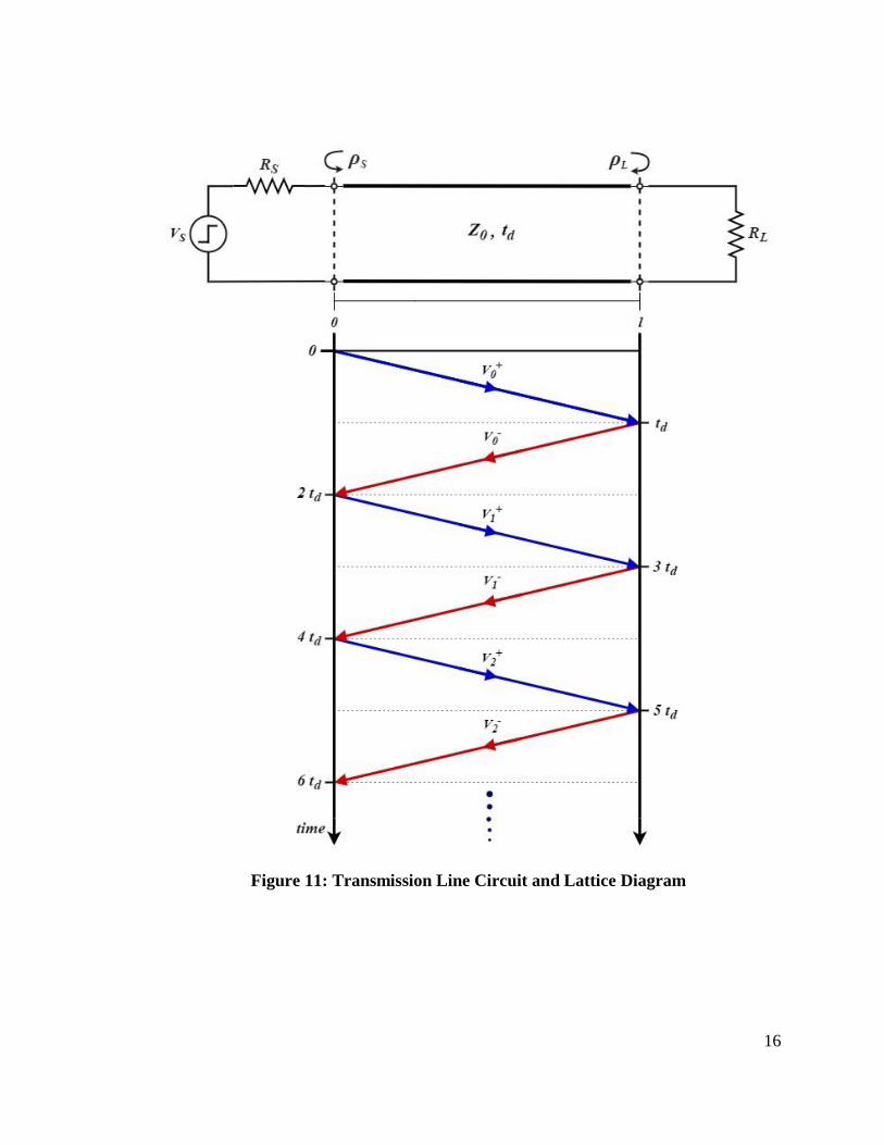
16
Figure 11: Transmission Line Circuit and Lattice Diagram

17
The blue arrow labeled 𝑉0+ indicates the first wave, or incident wave, that travels along the
transmission line. The incident voltage can be calculated using (1).
𝑉0+ = 𝑉𝑆 ·
𝑍0𝑅𝑆 + 𝑍0
(1)
After one propagation delay, 𝑡𝑑, the incident wave reaches the far end of the transmission
line and reflects off the load, sending another wave back towards the source. After an
additional propagation delay, this wave reaches the source and creates another reflection.
This process continues indefinitely if the source resistance, 𝑅𝑆, and load resistance, 𝑅𝐿, are
not matched to the characteristic impedance of the line, 𝑍0.
Each time a reflection occurs, the reflected wave has a magnitude that is equal to the
incoming wave multiplied by a reflection coefficient. The source and load each have their
own reflection coeffects that can be calculated using (2) and (3), respectively.
𝜌𝑆 =𝑅𝑆 − 𝑍0𝑅𝑆 + 𝑍0
(2)
𝜌𝐿 =𝑅𝐿 − 𝑍0𝑅𝐿 + 𝑍0
(3)
The voltages and currents across the transmission line for a given time can be calculated
by summing up all the forward and backward traveling waves up to that point in time. A

18
transmission line reaches steady state when the contributions of the reflected waves are
negligible compared to the overall signal on the line.
4.1.2 General Transmission Line Circuit Model
The objective of the transmission line circuit model is to generate animation data that will
be used in the Interactive Tool for Teaching Transmission Line Concepts. This tool
supports animations of the voltages and currents across the length of the transmission line,
as well as at the ends. To create the transient and steady state animations, two separate
models were developed. Both models support some common sources and the same loads.
The sources that are available in this model include step, ramped step, and transient
sinusoidal sources, which can be seen in Figure 12, Figure 13, and Figure 14, respectively.
The loads that are supported are illustrated in Figure 15.
Figure 12: Step Source

19
Figure 13: Ramped Step Source
Figure 14: Transient Sinusoidal Source
All the sources have an amplitude, 𝐴. Additionally, the ramped step source has a rise time,
𝑡𝑟, and the sinusoidal source has a frequency, 𝑓.

20
Figure 15: Supported Loads
The transient transmission line model supports all the sources described above and the
steady state model supports a sinusoidal source. The reason the steady state model does not
provide animations for the step and ramped step sources is because the signals across the
line are simply constant at steady state. While both models support many of the same
sources and loads, separate equations are used to generate the data for the transient and
steady state animations. The differences between the transient and steady state models are
discussed below.
21
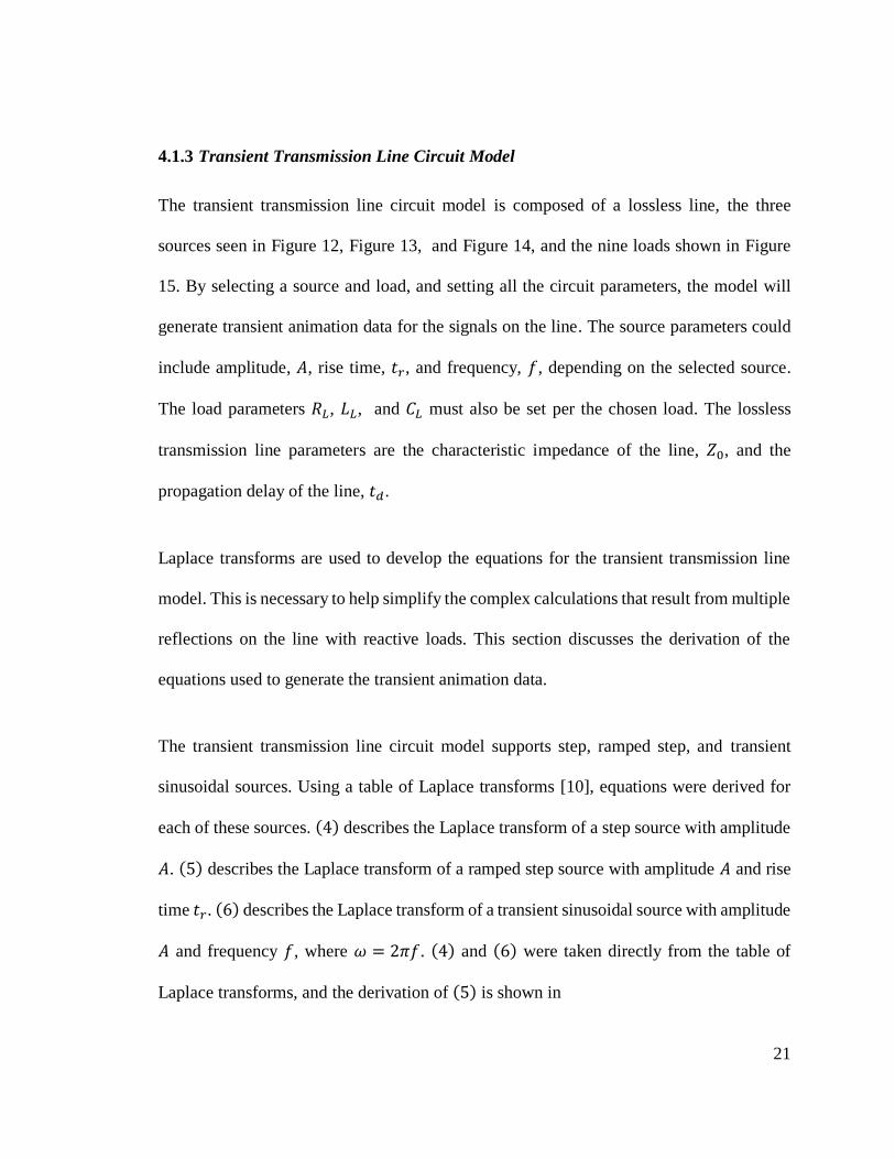
4.1.3 Transient Transmission Line Circuit Model
The transient transmission line circuit model is composed of a lossless line, the three
sources seen in Figure 12, Figure 13, and Figure 14, and the nine loads shown in Figure
15. By selecting a source and load, and setting all the circuit parameters, the model will
generate transient animation data for the signals on the line. The source parameters could
include amplitude, 𝐴, rise time, 𝑡𝑟, and frequency, 𝑓, depending on the selected source.
The load parameters 𝑅𝐿, 𝐿𝐿, and 𝐶𝐿 must also be set per the chosen load. The lossless
transmission line parameters are the characteristic impedance of the line, 𝑍0, and the
propagation delay of the line, 𝑡𝑑.
Laplace transforms are used to develop the equations for the transient transmission line
model. This is necessary to help simplify the complex calculations that result from multiple
reflections on the line with reactive loads. This section discusses the derivation of the
equations used to generate the transient animation data.
The transient transmission line circuit model supports step, ramped step, and transient
sinusoidal sources. Using a table of Laplace transforms [10], equations were derived for
each of these sources. (4) describes the Laplace transform of a step source with amplitude
𝐴. (5) describes the Laplace transform of a ramped step source with amplitude 𝐴 and rise
time 𝑡𝑟. (6) describes the Laplace transform of a transient sinusoidal source with amplitude
𝐴 and frequency 𝑓, where 𝜔 = 2𝜋𝑓. (4) and (6) were taken directly from the table of
Laplace transforms, and the derivation of (5) is shown in

22
Appendix A.
𝑉𝑆(𝑠) = 𝐴 ·1
𝑠 (4)
𝑉𝑆(𝑠) =𝐴
𝑡𝑟·1
𝑠2· (1 − 𝑒−𝑡𝑟·𝑠) (5)
𝑉𝑆(𝑠) = 𝐴 ·𝜔
𝑠2 +𝜔2 (6)
The loads that are supported by this model are illustrated in Figure 15. To calculate the
load impedance, 𝑍𝐿, the s-domain impedances of 𝑅𝐿, 𝐿𝐿, and 𝐶𝐿 must be used. The load
impedance calculations for each load configuration are illustrated in Table 1.

23
Table 1: s-Domain Load Impedances
Load Configuration Load Impedance, 𝒁𝑳
Resistor 𝑹𝑳
Inductor 𝒔𝑳𝑳
Capacitor 𝟏
𝒔𝑪𝑳
Series Resistor & Inductor 𝑹𝑳 + 𝒔𝑳𝑳
Series Resistor & Capacitor 𝑹𝑳 +𝟏
𝒔𝑪𝑳
Series Resistor, Inductor & Capacitor 𝑹𝑳 + 𝒔𝑳𝑳 +𝟏
𝒔𝑪𝑳
Parallel Resistor & Inductor (𝟏
𝑹𝑳+
𝟏
𝒔𝑳𝑳)−𝟏
Parallel Resistor & Capacitor (𝟏
𝑹𝑳+ 𝒔𝑪𝑳)
−𝟏
Parallel Resistor, Inductor & Capacitor (𝟏
𝑹𝑳+
𝟏
𝒔𝑳𝑳+ 𝒔𝑪𝑳)
−𝟏

24
To generate the animation data for the transient transmission line model, several equations
were developed using the concepts discussed in Section 4.1.1. Figure 16 shows a
transmission line circuit and the corresponding s-domain lattice diagram. All variables
illustrated in this figure are operational s-domain parameters. The reflection coefficients,
𝜌𝑆 and 𝜌𝐿, that were used in Section 4.1.1 have been changed to Γ𝑆 and Γ𝐿 to signify that
they are operational parameters. The equations for Γ𝑆 and Γ𝐿 can be seen in (7) and (8),
respectively.
𝛤𝑆(𝑠) =𝑍𝑆 − 𝑍0𝑍𝑆 + 𝑍0
(7)
𝛤𝐿(𝑠) =𝑍𝐿 − 𝑍0𝑍𝐿 + 𝑍0
(8)
The s-domain voltage that is entering the near end of the transmission line, 𝑉0+, is illustrated
in (9).
𝑉0+(𝑠) = 𝑉𝑆(𝑠) ·
𝑍0𝑍𝑆 + 𝑍0
(9)
It is also necessary to derive an operational s-domain equation for the traveling waves on
the transmission line. The solution for voltage phasor of the forward going wave is shown
in (10) [11], where 𝑉+ is a complex constant determined by the boundary of 𝑍𝑆 and 𝑍0, 𝛾
is the propagation constant, and 𝑧 is the location on the transmission line.
25
𝑉+𝑒−𝛾𝑧 (10)
The formula for 𝛾 on a lossless transmission line is illustrated in (11), where 𝐿 is the
inductance per meter on the transmission line, and 𝐶 is the capacitance per meter on the
line.
𝛾 = √(𝑗𝜔𝐿)(𝑗𝜔𝐶) (11)
To create the operational s-domain form of 𝛾, the 𝑗𝜔 terms in (11) can be substituted with
the Laplace operator, 𝑠, as shown in (12) [12].
𝛾(𝑠) = 𝑠√𝐿𝐶 (12)
Combining (9), (10), and (13), the operational solution for the forward going wave, 𝑉𝑓,
as a function of distance can be derived, as illustrated in (13).
𝑉𝑓(𝑧, 𝑠) = 𝑉+(𝑠)𝑒−𝑠√𝐿𝐶·𝑧 (13)
Since 𝑣𝑃 =1
√𝐿𝐶 for a lossless line [13], and 𝑡𝑑 =
𝑙
𝑣𝑝, evaluating (13) at 𝑧 = 𝑙 provides an
equation for 𝑉𝑓 at the end of the transmission line in terms of 𝑡𝑑. This equation is illustrated
in (14).
𝑉𝑓(𝑙, 𝑠) = 𝑉+(𝑠)𝑒−𝑠√𝐿𝐶·𝑙 = 𝑉+(𝑠)𝑒
−𝑠·𝑙𝑉𝑃 = 𝑉+(𝑠)𝑒−𝑠·𝑡𝑑 (14)

26
To develop the equations for the signals at the ends of the transmission line, the operational
propagation factor, 𝑝, is used to characterize how a signal has changed after traveling from
one end of the transmission line to the other. Using the equation developed in (14), 𝑝 is
defined as shown in (15).
𝑝(𝑠) = 𝑒−𝑠·𝑡𝑑 (15)
Figure 16: Transmission Line Circuit and s-Domain Lattice Diagram

27
Calculating the Transient Voltage at the Near End of the Line
The near end of the transmission line refers to the end nearest to the source. The voltage at
the near end, 𝑉𝑁𝐸, is depicted in the circuit shown in Figure 16. To calculate 𝑉𝑁𝐸 for a given
time, the sum of all incoming and outgoing waves at the near end is taken up to that point
in time. (16) illustrates this process.
𝑉𝑁𝐸(𝑠) =
{
𝑉0+ 0 ≤ 𝑡 < 2𝑡𝑑
𝑉0+ + 𝑉0
+𝑝2𝛤𝐿 + 𝑉0+𝑝2𝛤𝐿𝛤𝑆 2𝑡𝑑 ≤ 𝑡 < 4𝑡𝑑
𝑉0+ + 𝑉0
+𝑝2𝛤𝐿 + 𝑉0+𝑝2𝛤𝐿𝛤𝑆 + 𝑉0
+𝑝4𝛤𝐿2𝛤𝑆 + 𝑉0
+𝑝4𝛤𝐿2𝛤𝑆
2 4𝑡𝑑 ≤ 𝑡 < 6𝑡𝑑
⋮ ⋮
(16)
By grouping like terms, (16) can be rewritten as shown in (17). From this consolidation,
a pattern starts to emerge as successive incoming and outgoing waves are added to 𝑉𝑁𝐸.
𝑉𝑁𝐸(𝑠) =
{
𝑉0+ 0 ≤ 𝑡 < 2𝑡𝑑
𝑉0+ · [ 1 + 𝑝2𝛤𝐿(1 + 𝛤𝑆) ] 2𝑡𝑑 ≤ 𝑡 < 4𝑡𝑑
𝑉0+ · [ 1 + 𝑝2𝛤𝐿(1 + 𝛤𝑆)(1 + 𝑝
2𝛤𝐿𝛤𝑆) ] 4𝑡𝑑 ≤ 𝑡 < 6𝑡𝑑
𝑉0+ · [ 1 + 𝑝2𝛤𝐿(1 + 𝛤𝑆)(1 + 𝑝
2𝛤𝐿𝛤𝑆 + 𝑝4𝛤𝐿
2𝛤𝑆2) ] 6𝑡𝑑 ≤ 𝑡 < 8𝑡𝑑
⋮ ⋮
(17)

28
The generalized version of (17) in terms of 𝑉0+ is shown in (18), where 𝑡𝑠 represents the
last time for which 𝑉𝑁𝐸 will be computed and ⌊ ⌋ represents the floor function, which rounds
the argument to the next lowest integer value.
𝑉𝑁𝐸(𝑠) = 𝑉0+ ·
[
1 + 𝛤𝐿 · (1 + 𝛤𝑆) · ∑ 𝑝𝑘 · (𝛤𝐿 · 𝛤𝑆)𝑘2−1
⌊𝑡𝑠𝑡𝑑⌋
𝑘=2,4,6…]
(18)
Since all voltage sources have already been defined in the s-domain, it is useful to represent
𝑉0+ in terms of the source voltage, 𝑉𝑆, and the source reflection coefficient, Γ𝑆. By
manipulating (7) and (1), 𝑉0+ can be rewritten as shown in (19).
𝑉0+(𝑠) =
𝑉𝑆(𝑠)
2· (1 − 𝛤𝑆) (19)
Substituting (19) into (18) gives the generalized equation for 𝑉𝑁𝐸 in terms of 𝑉𝑆, which is
illustrated in (20).
𝑉𝑁𝐸(𝑠) =𝑉𝑆(𝑠)
2· (1 − 𝛤𝑆) ·
[
1 + 𝛤𝐿 · (1 + 𝛤𝑆) · ∑ 𝑝𝑘 · (𝛤𝐿 · 𝛤𝑆)𝑘2−1
⌊𝑡𝑠𝑡𝑑⌋
𝑘=2,4,6…]
(20)
To get the time domain equation for the voltage at the near end of the transmission line,
𝑣𝑁𝐸(𝑡), the inverse Laplace transform of 𝑉𝑁𝐸 is taken, as shown in (21).
𝑣𝑁𝐸(𝑡) = ℒ−1{𝑉𝑁𝐸(𝑠)} (21)

29
Calculating the Transient Voltage at the Far End of the Line
The far end of the transmission line refers to the end nearest to the load. Calculating the
voltage at the far end, 𝑉𝐹𝐸, for a given time uses the same approach taken to calculate 𝑉𝑁𝐸,
but the sum of the incoming and outgoing waves is taken from the far end of the line.
Following the same process, the generalized equation for 𝑉𝐹𝐸 in terms of 𝑉𝑆 can be
calculated. The result of this calculation is shown in (22).
𝑉𝐹𝐸(𝑠) =𝑉𝑆(𝑠)
2· (1 − 𝛤𝑆) ·
[
(1 + 𝛤𝐿) · ∑ 𝑝𝑘 · (𝛤𝐿 · 𝛤𝑆)𝑘−12
⌊𝑡𝑠𝑡𝑑⌋
𝑘=1,3,5,…]
(22)
The time domain equation for the voltage at the far end of the line, 𝑣𝐹𝐸(𝑡), can then be
calculated by taking the inverse Laplace transform of 𝑉𝐹𝐸, as shown in (23).
𝑣𝐹𝐸(𝑡) = ℒ−1{𝑉𝐹𝐸(𝑠)} (23)

30
Calculating the Transient Current at the Near End of the Line
Calculating the current at the near end of the line, 𝐼𝑁𝐸, for a given time uses the same
process that was used for 𝑉𝑁𝐸, but the source reflection coefficient for current is −Γ𝑆 and
the load reflection coefficient for current is −Γ𝐿. The calculation for 𝐼𝑁𝐸 also uses the
incident current wave, 𝐼0+, as opposed to 𝑉0
+. The calculation for 𝐼0+ is shown in (24).
𝐼0+(𝑠) =
𝑉0+(𝑠)
𝑍0(24)
It is useful to represent 𝐼0+ in terms of 𝑉𝑆, just as it was useful to represent 𝑉0
+ in terms of
𝑉𝑆. By manipulating (19) and (24), 𝐼0+ can be rewritten as shown in (19).
𝐼0+ =
𝑉𝑆2𝑍0
· (1 − 𝛤𝑆) (25)
Following the same process that was used to calculate 𝑉𝑁𝐸 and applying the changes that
were described above, the generalized equation for 𝐼𝑁𝐸 in terms of 𝑉𝑆 is calculated using
equation (26).
𝐼𝑁𝐸(𝑠) =𝑉𝑆(𝑠)
2𝑍0· (1 − 𝛤𝑆) ·
[
1 − 𝛤𝐿 · (1 − 𝛤𝑆) · ∑ 𝑝𝑘 · (𝛤𝐿 · 𝛤𝑆)𝑘2−1
⌊𝑡𝑠𝑡𝑑⌋
𝑘=2,4,6…]
(26)

31
The time domain equation for the current at the near end of the transmission line, 𝑖𝑁𝐸(𝑡),
is calculated by taking the inverse Laplace transform of 𝐼𝑁𝐸, as shown in (27).
𝑖𝑁𝐸(𝑡) = ℒ−1{𝐼𝑁𝐸(𝑠)} (27)

32
Calculating the Transient Current at the Far End of the Line
Calculating the transient current at the far end of the line, 𝐼𝐹𝐸, for a given time follows the
same steps used to calculate 𝐼𝑁𝐸, but the incoming and outgoing waves are summed at the
far end of the line. Following this process, the generalized equation for 𝐼𝐹𝐸 in terms of 𝑉𝑆
is illustrated in (28).
𝐼𝐹𝐸(𝑠) =𝑉𝑆(𝑠)
2𝑍0· (1 − 𝛤𝑆) ·
[
(1 − 𝛤𝐿) · ∑ 𝑝𝑘 · (𝛤𝐿 · 𝛤𝑆)𝑘−12
⌊𝑡𝑠𝑡𝑑⌋
𝑘=1,3,5,…]
(28)
Generating the time domain equation for the current at the far end of the transmission line,
𝑖𝐹𝐸(𝑡), involves taking the inverse Laplace transform of 𝐼𝐹𝐸, as shown in (29).
𝑖𝐹𝐸(𝑡) = ℒ−1{𝐼𝐹𝐸(𝑠)} (29)

33
Calculating the Forward Traveling Voltage Wave Leaving the Near End of the Line
To compute the overall voltage across the transmission line, it is useful to derive an
equation that describes the overall forward traveling voltage wave leaving from the near
end of the line, 𝑉𝑓,𝑁𝐸. This equation is used to generate the animation of the voltage across
the transmission line and is described in more detail in Section 4.2.2. To calculate 𝑉𝑓,𝑁𝐸 for
a given time, the summation of all outgoing waves at the near end of the line is taken up to
that point in time. This uses the same procedure that was used to calculate 𝑉𝑁𝐸, but the
contributions of the incoming waves are not included. Following this process, the general
equation for 𝑉𝑓,𝑁𝐸 in terms of 𝑉𝑆 is illustrated in (30).
𝑉𝑓,𝑁𝐸(𝑠) =𝑉𝑆(𝑠)
2· (1 − 𝛤𝑆) ·
[
1 + ∑ 𝑝𝑘 · (𝛤𝐿 · 𝛤𝑆)𝑘2
⌊𝑡𝑠𝑡𝑑⌋
𝑘=2,4,6…]
(30)
Generating the time domain equation for the forward traveling voltage wave leaving the
near end of the line, 𝑣𝑓,𝑁𝐸(𝑡), is accomplished by taking the inverse Laplace transform of
𝑉𝑓,𝑁𝐸, as shown in (31).
𝑣𝑓,𝑁𝐸(𝑡) = ℒ−1{𝑉𝑓,𝑁𝐸(𝑠)} (31)

34
Calculating the Backward Traveling Voltage Wave Leaving the Far End of the Line
To compute the overall voltage on the transmission line, it is also useful to derive an
equation for the backward traveling voltage wave that is leaving from the far end of the
line, 𝑉𝑏,𝐹𝐸. This equation is also used to generate the animation of the voltage across the
transmission line and is described in more detail in Section 4.2.2. To calculate 𝑉𝑏,𝐹𝐸 for a
given time, all outgoing waves at the far end are summed up to that point in time. Deriving
the general equation for 𝑉𝑏,𝐹𝐸 in terms of 𝑉𝑆 uses the same process that is described in the
above sections. The result is illustrated in (32).
𝑉𝑏,𝐹𝐸(𝑠) =𝑉𝑆(𝑠)
2· (1 − 𝛤𝑆) ·
[
𝛤𝐿 · ∑ 𝑝𝑘 · (𝛤𝐿 · 𝛤𝑆)𝑘−12
⌊𝑡𝑠𝑡𝑑⌋
𝑘=1,3,5,…]
(32)
The time domain equation for the backward traveling voltage wave leaving from the far
end of the line, 𝑣𝑏,𝐹𝐸(𝑡) can be generated by taking the inverse Laplace transform of 𝑉𝑏,𝐹𝐸,
as shown in (33).
𝑣𝑏,𝐹𝐸(𝑡) = ℒ−1{𝑉𝑏,𝐹𝐸(𝑠)} (33)
35
4.1.4 Steady State Transmission Line Circuit Model
The steady state transmission line circuit model is composed of a lossy line, a sinusoidal
source, and the nine loads shown in Figure 15. By selecting a load and setting all the circuit
parameters, the model will generate steady state animation data for the signals on the line.
The source parameters include amplitude, 𝐴, and frequency, 𝑓. The load parameters 𝑅𝐿,
𝐿𝐿, and 𝐶𝐿 must be set per the chosen load, and the load impedance, 𝑍𝐿, can be calculated
using Table 2. The lossy transmission line parameters include the inductance per unit
length, 𝐿, capacitance per unit length, 𝐶, resistance per unit length, 𝑅, conductance per unit
length, 𝐺, and the length of the line, 𝑙. In addition to these circuit parameters, several other
derived parameters are used to develop the equations for this model [11]. These parameters
include:
Angular frequency of the source, 𝜔, (34)
Characteristic impedance of the line, 𝑍0, (35)
Propagation constant, 𝛾, (36)
𝜔 = 2𝜋𝑓 (34)
𝑍0 = √𝑅 + 𝑗𝜔𝐿
𝐺 + 𝑗𝜔𝐶(35)
𝛾 = √(𝑅 + 𝑗𝜔𝐿)(𝐺 + 𝑗𝜔𝐶) (36)

36
Table 2: Complex Load Impedances
Load Configuration Load Impedance, 𝒁𝑳
Resistor 𝑹𝑳
Inductor 𝒋𝝎𝑳𝑳
Capacitor 𝟏
𝒋𝝎𝑪𝑳
Series Resistor & Inductor 𝑹𝑳 + 𝒋𝝎𝑳𝑳
Series Resistor & Capacitor 𝑹𝑳 +𝟏
𝒋𝝎𝑪𝑳
Series Resistor, Inductor & Capacitor 𝑹𝑳 + 𝒋𝝎𝑳𝑳 +𝟏
𝒋𝝎𝑪𝑳
Parallel Resistor & Inductor (𝟏
𝑹𝑳+
𝟏
𝒋𝝎𝑳𝑳)−𝟏
Parallel Resistor & Capacitor (𝟏
𝑹𝑳+ 𝒋𝝎𝑪𝑳)
−𝟏
Parallel Resistor, Inductor & Capacitor (𝟏
𝑹𝑳+
𝟏
𝒋𝝎𝑳𝑳+ 𝒋𝝎𝑪𝑳)
−𝟏

37
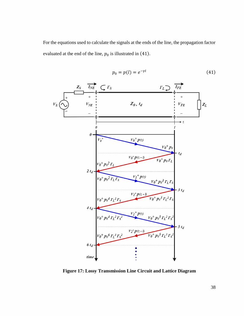
To generate the animation data for the steady state transmission line model, several
equations were developed using the concepts discussed in Section 4.1.1. Figure 17 shows
a transmission line circuit and lattice diagram for general lossy lines that is similar to the
illustrations shown in Figure 11. All parameters shown in Figure 17 represent phasors.
The incident voltage, 𝑉0+ shown in (37), is a phasor that represents voltage entering the
transmission line.
𝑉0+ = 𝑉𝑆 ·
𝑍0𝑍𝑆 + 𝑍0
(37)
The source and load reflection coefficient phasors represented by Γ𝑆 and Γ𝐿, can be seen in
(38) and (39), respectively.
𝛤𝑆 =𝑍𝑆 − 𝑍0𝑍𝑆 + 𝑍0
(38)
𝛤𝐿 =𝑍𝐿 − 𝑍0𝑍𝐿 + 𝑍0
(39)
On lossy transmission lines, signals decay, in addition to undergoing a decreasing phase
change as they move across the line. The propagation factor, 𝑝, shown in (40), represents
the change in amplitude and phase that signals undergo as a function of distance.
𝑝(𝑧) = 𝑒−𝛾𝑧 (40)
38
For the equations used to calculate the signals at the ends of the line, the propagation factor
evaluated at the end of the line, 𝑝0 is illustrated in (41).
𝑝0 = 𝑝(𝑙) = 𝑒−𝛾𝑙 (41)
Figure 17: Lossy Transmission Line Circuit and Lattice Diagram
39
Calculating the Steady State Voltage at the Near End of the Line
Calculating the steady state voltage at the near end of the line, 𝑉𝑁𝐸, involves summing all
incoming and outgoing waves at the near end of the line as 𝑡 → ∞. (42) illustrates this
process.
𝑉𝑁𝐸 = 𝑉0+ + 𝑉0
+𝑝02𝛤𝐿 + 𝑉0
+𝑝02𝛤𝐿𝛤𝑆 + 𝑉0
+𝑝04𝛤𝐿
2𝛤𝑆 + 𝑉0+𝑝0
4𝛤𝐿2𝛤𝑆
2 +⋯ (42)
By grouping like terms, (42) is rewritten as shown in (43).
𝑉𝑁𝐸 = 𝑉0+ · [1 + 𝑝0
2𝛤𝐿 · (1 + 𝛤𝑆) · (1 + 𝑝02𝛤𝐿𝛤𝑆 + 𝑝0
4𝛤𝐿2𝛤𝑆
2 + ⋯)] (43)
The infinite sum in (43) can then be rewritten as (44).
𝑉𝑁𝐸 = 𝑉0+ · [1 + 𝑝0
2𝛤𝐿 · (1 + 𝛤𝑆) ·∑(𝑝02𝛤𝐿𝛤𝑆)
𝑘
∞
𝑘=0
] (44)
Since |𝑝02Γ𝐿Γ𝑆| < 1, the geometric series [14] illustrated in (45) can be used with (44) to
create the closed form solution for 𝑉𝑁𝐸, shown in (46).
∑𝑥𝑘∞
𝑘=0
= {
1
1 − 𝑥|𝑥| < 1
𝐷𝑖𝑣𝑒𝑟𝑔𝑒𝑠 |𝑥| ≥ 1
(45)
𝑉𝑁𝐸 = 𝑉0+ · [1 +
𝑝02𝛤𝐿 · (1 + 𝛤𝑆)
1 − 𝑝02𝛤𝐿𝛤𝑆
] (46)
40
To convert a phasor to the time domain, (47) can be used, where 𝑉 is a phasor and 𝑣(𝑡) is
the time domain representation of the phasor [15].
𝑣(𝑡) = 𝑅𝑒{𝑉 · 𝑒𝑗𝜔𝑡} (47)
Substituting 𝑉𝑁𝐸 into (47), the time domain representation 𝑣𝑁𝐸(𝑡), can be computed using
(48).
𝑣𝑁𝐸(𝑡) = 𝑅𝑒{𝑉𝑁𝐸 · 𝑒𝑗𝜔𝑡} (48)
41
Calculating the Steady State Voltage at the Far End of the Line
Calculating the steady state voltage at the far end of the line, 𝑉𝐹𝐸, involves summing all
incoming and outgoing waves at the far end of the line as 𝑡 → ∞. Generating the closed
form solution for the 𝑉𝐹𝐸 uses the same process that was used to calculate 𝑉𝑁𝐸. This result
is shown in (49).
𝑉𝐹𝐸 = 𝑉0+ · [
𝑝0 · (1 + 𝛤𝐿)
1 − 𝑝02𝛤𝐿𝛤𝑆
] (49)
To create the time domain representation 𝑣𝐹𝐸(𝑡), 𝑉𝐹𝐸 is substituted into (47) as illustrated
in (50).
𝑣𝐹𝐸(𝑡) = 𝑅𝑒{𝑉𝐹𝐸 · 𝑒𝑗𝜔𝑡} (50)
42
Calculating the Steady State Current at the Near End of the Line
Calculating the steady state current at the near end of the line, 𝐼𝑁𝐸, uses the same procedure
as described above, but the source and load reflection coefficients for current are −Γ𝑆 and
−Γ𝐿. The calculation for 𝐼𝑁𝐸 also uses the incident current wave, 𝐼0+, as opposed to 𝑉0
+. The
calculation for 𝐼0+ is shown in (24).
𝐼0+ =
𝑉0+
𝑍0(51)
Making the adjustments described above and following the same process used to calculate
𝑉𝑁𝐸, the closed form solution for 𝐼𝑁𝐸 is shown in (52).
𝐼𝑁𝐸 = 𝐼0+ · [
1 − 𝑝02𝛤𝐿
1 − 𝑝02𝛤𝐿𝛤𝑆
] (52)
Substituting 𝐼𝑁𝐸 into (47), the time domain equation for the current at the near end of the
line, 𝑖𝑁𝐸(𝑡), can be computed as illustrated in (53).
𝑖𝑁𝐸(𝑡) = 𝑅𝑒{𝐼𝑁𝐸 · 𝑒𝑗𝜔𝑡} (53)

43
Calculating the Steady State Current at the Far End of the Line
Using the same process that was used to calculate 𝐼𝑁𝐸, but summing all the incoming and
outgoing waves at the far end of the line, the closed form solution for the current at the far
end of the line, 𝐼𝐹𝐸, is shown in (54).
𝐼𝐹𝐸 = 𝐼0+ · [
𝑝0 · (1 − 𝛤𝐿)
1 − 𝑝02𝛤𝐿𝛤𝑆
] (54)
The time domain equation for the current at the far end of the line, 𝑖𝐹𝐸(𝑡), can be calculated
by substituting 𝐼𝐹𝐸 into (47), as shown in (55).
𝑖𝐹𝐸(𝑡) = 𝑅𝑒{𝐼𝐹𝐸 · 𝑒𝑗𝜔𝑡} (55)

44
Calculating the Steady State Voltage Across the Line
The voltage phasor as a function of distance along a lossy transmission line, 𝑉(𝑧), can be
calculated by multiplying all forward traveling waves, 𝑉𝑘+, and backward traveling waves,
𝑉𝑘−, by the propagation factor, 𝑝(𝑧), and summing as 𝑡 → ∞. The general equation for 𝑉(𝑧)
is illustrated in (56).
𝑉(𝑧) = 𝑝(𝑧) ·∑𝑉𝑘+
∞
𝑘=0
+ 𝑝(𝑧 − 𝑙) ·∑𝑉𝑘−
∞
𝑘=0
(56)
The sum of all forward traveling waves is shown in (57) and the sum of all backward
traveling waves is shown in (58).
∑𝑉𝑘+
∞
𝑘=0
= 𝑉0+ · ∑(𝑝0
2Γ𝐿Γ𝑆)𝑘
∞
𝑘=0
(57)
∑𝑉𝑘−
∞
𝑘=0
= 𝑉0+𝑝0Γ𝐿 ·∑(𝑝0
2Γ𝐿Γ𝑆)𝑘
∞
𝑘=0
(58)
Since |𝑝2Γ𝐿Γ𝑆| < 1, the geometric series described in (45) can be used with equations (57)
and (58) to create closed form solutions for the summations of all forward and backward
traveling waves. These solutions can be seen in (59) and (60), respectively.
∑𝑉𝑘+
∞
𝑘=0
=𝑉0+
1 − 𝑝02Γ𝐿Γ𝑆
(59)

45
∑𝑉𝑘−
∞
𝑘=0
= 𝑉0+𝑝0Γ𝐿
1 − 𝑝02Γ𝐿Γ𝑆
(60)
Substituting the closed form solutions for the traveling waves shown in (59) and (60) into
the general equation for 𝑉(𝑧) in (56), the closed form representation of 𝑉(𝑧) can be
calculated as shown in (61).
𝑉(𝑧) = 𝑉0+ · [
𝑝(𝑧)
1 − 𝑝02𝛤𝐿𝛤𝑆
+ 𝑝(𝑧 − 𝑙) · 𝑝0𝛤𝐿1 − 𝑝0
2𝛤𝐿𝛤𝑆] (61)
The time domain equation for the voltage as a function of distance across the line, 𝑣(𝑧, 𝑡),
can be calculated by substituting 𝑉(𝑧) into (47), as shown in (62).
𝑣(𝑡, 𝑧) = 𝑅𝑒{𝑒𝑗𝜔𝑡 · 𝑉(𝑧)} (62)
When generating the animation data in the following Section (4.2.2), the voltage across the
line is represented as a 2-dimensional array, [𝑣]. To calculate [𝑣], (63) can be used, where
𝑡 is a column vector representing each instant of the simulation time, 𝑧 is a row vector
representing each position on the line, and ⊗ is the tensor product.
[𝑣] = 𝑅𝑒{𝑒𝑗𝜔𝑡⊗𝑉(𝑧)} (63)

46
Calculating the Steady State Current Across the Line
Calculating the current phasor as a function of distance along a lossy transmission line,
𝐼(𝑧), requires the same steps used to calculate the steady state voltage, but the reflection
coefficients for current, −Γ𝑆 and −Γ𝐿, are used, and the incident current wave, 𝐼0+, is used.
The closed form solution for 𝐼(𝑧) is shown in (64).
𝐼(𝑧) = 𝐼0+ · [
𝑝(𝑧)
1 − 𝑝02𝛤𝐿𝛤𝑆
− 𝑝(𝑧 − 𝑙) · 𝑝0𝛤𝐿1 − 𝑝0
2𝛤𝐿𝛤𝑆] (64)
The time domain equation for the current as a function of distance across the line, 𝑖(𝑧, 𝑡),
can be calculated by substituting 𝐼(𝑧) into (47), as shown in (55).
𝑖(𝑡, 𝑧) = 𝑅𝑒{𝑒𝑗𝜔𝑡 · 𝐼(𝑧)} (65)
When generating the animation data for the current across the line, [𝑖], (66) can be used,
where 𝑡 is a column vector representing each instant of the simulation time, 𝑧 is a row
vector representing each position on the line, and ⊗ is the tensor product.
[𝑖] = 𝑅𝑒{𝑒𝑗𝜔𝑡⊗ 𝐼(𝑧)} (66)

47
Calculating the Standing Wave Pattern of the Signals Across the Line
Calculating the standing wave pattern of the signals across the transmission line can be
accomplished by taking the magnitude of the voltage phasor, 𝑉(𝑧), and current phasor,
I(z), that were developed in (61) and (64), respectively.

48
4.2 Implementation
4.2.1 Development Platform
The Interactive Tool for Teaching Transmission Line Concepts was developed using
Matlab. Matlab was chosen because it is accessible to students, it is well suited for
mathematical operations, and it provides many tools for creating aesthetically pleasing user
interfaces.
4.2.2 Animations
The first step in generating the animations in Matlab is to create a time column vector, 𝒕. 𝒕
spans from 0 up to the stop time of the simulation, 𝑡𝑠, and has 𝑁 elements. (67) describes
the time column vector 𝒕.
𝒕 =
[ 𝑡1
𝑡2
⋮
𝑡𝑁]
, 𝑤ℎ𝑒𝑟𝑒 𝑡𝑛 =(𝑛 − 1) · 𝑡𝑠𝑁 − 1
(67)
The number of elements, 𝑁, that are used to create 𝑡 is controlled by a precision parameter,
𝑀. 𝑀 represents the number of points per propagation delay, 𝑡𝑑, in the simulation. 𝑁 is
calculated using (68), where ⌈ ⌉ is the ceiling function, which rounds the argument to the
next highest integer value. 𝑀 is set to 100 by default, but can be adjusted by the user in the
transmission line tool.

49
𝑁 = ⌈𝑀 ·𝑡𝑠𝑡𝑑⌉ (68)
Another vector that is used when creating the animations across the length of the
transmission line is the distance vector, 𝒛. 𝒛 is a row vector that spans from 0 to the length
of the line, 𝑙, and has 𝑀 elements. The vector 𝒛 is illustrated in (69).
𝒛 = [𝑧1 𝑧2 … 𝑧𝑀], 𝑤ℎ𝑒𝑟𝑒 𝑧𝑛 =(𝑛 − 1) · 𝑙
𝑀 − 1(69)
To ensure that the transient and steady state animations can use the same code in Matlab,
all the animation data are put into the same format. This tool provides animations of the
signals at the ends of the transmission line as well as across the line. The animation data
for the signals at the ends of the line are the same dimensions as the time vector, 𝒕. The
animation data for the signals across the line are formatted in an (𝑁 𝑥 𝑀) 2-dimensional
array, where the rows represent each instant of the simulation time and the columns
represent locations along the transmission line. The data format for the signals across the
line is illustrated in (70), where 𝑥 represents a generic signal.
[𝑥] =
[ 𝑥(𝑡1, 𝑧1) ⋯ 𝑥(𝑡1, 𝑧𝑀)
⋮ ⋱ ⋮
𝑥(𝑡𝑁, 𝑧1) ⋯ 𝑥(𝑡𝑁, 𝑧𝑀)]
(70)

50
The following section describes how the animation data is developed for each of the signals
and how the animations are created.
51
Generating Animation Data for the Signals at the Ends of the Line
Both the transient and steady state models use the same approach to generate animation
data for the signals at the ends of the line. The equations used to calculate these signals,
𝑣𝑛𝑒(𝑡), 𝑖𝑛𝑒(𝑡), 𝑣𝑓𝑒(𝑡), and 𝑖𝑓𝑒(𝑡), were developed in Sections 4.1.3 and 4.1.4. By
evaluating each of these equations using the time vector, 𝒕, the signals at each instant in
time during the simulation can be calculated.

52
Generating Transient Animation Data for the Signals Across the Line
Generating the transient animation data for the signals across the transmission line uses the
equations, 𝑣𝑓,𝑁𝐸(𝑡) and 𝑣𝑏,𝐹𝐸(𝑡), that were developed in Section 4.1.3. To calculate the
voltage across the line for a given time, the forward and backwards traveling voltage
waves, 𝑣𝑓(𝑡, 𝑧) and 𝑣𝑏(𝑡, 𝑧), must be calculated. Both 𝑣𝑓(𝑡, 𝑧) and 𝑣𝑏(𝑡, 𝑧) are represented
as 2-dimensional arrays in Matlab and are in the form shown in (70). To create the forward
and backward traveling voltage arrays, [𝑣𝑓] and [𝑣𝑏], a shift register technique is used
along with 𝑣𝑓,𝑁𝐸(𝑡) and 𝑣𝑏,𝐹𝐸(𝑡). Figure 18 and Figure 19 illustrate how this animation
data is generated. The Matlab code for this can be seen in Appendix B. The transient
animation data for the voltage across the transmission line, [𝑣], can be calculated as
illustrated in (71).
[𝑣] = [𝑣𝑓] + [𝑣𝑏] (71)

53
Figure 18: Forward Traveling Voltage Wave for Transient Animation

54
Figure 19: Backward Traveling Voltage Wave for Transient Animation
To generate the animation data for the current across the line, [𝑖], the forward and backward
traveling currents, [𝑖𝑓] and [𝑖𝑏], must first be computed using (72) and (73).
[𝑖𝑓] =[𝑣𝑓]
𝑍0(72)
[𝑖𝑏] = −[𝑣𝑏]
𝑍0(73)
The animation data, [𝑖], can then be calculated using (74).

55
[𝑖] = [𝑖𝑓] + [𝑖𝑏] (74)
Generating Steady State Animation Data for Signals Across the Line
To generate the steady state animation data for the voltage and current across the line, [𝑣]
and [𝑖], (63) and (66) that were developed in Section 4.1.4 can be used with the vectors 𝒕
and 𝒛, that were described above. This produces 2-dimensional arrays of the voltage and
current across the line at different instants in time. These arrays are in the same format
illustrated in (70).
One of the features that this tool provides is the ability to plot the standing wave pattern of
the signals across the transmission line for steady state animations. To generate the
standing wave pattern for the voltage and the current across the line, the distance vector, 𝒛,
can be substituted into (61) and (64), respectively, and the magnitudes are taken.

56
Generating the Animations
This tool supports animations of the signals across the transmission line, as well as at each
end of the line. The data for the signals across the line are formatted in 2-dimensional
arrays, where the rows are instants in time and the columns are locations on the
transmission line. Animations of the signals across the line are created by iterating through
each row and plotting all the columns in that row. An example of the Matlab code that is
used to generate the animations of the signals across the line is provided in Appendix C.
The data for the signals at the ends of the line are formatted in 1-dimensional arrays, where
each element of the array represents the signals value at a specific point in time. Animations
of the signals at each end of the line are created by iterating through each element of the
animation data and adding that element to the plot. An example of the Matlab code that is
used to generate the animations of the signals at the ends of the line is provided in Appendix
D.

57
4.2.3 User Interface
The goal when designing the user interface was to make it easy for students to understand.
By displaying an editable circuit diagram, as shown in Figure 20 and Figure 21, students
can adjust the circuit parameters as they wish, with little to no training. All parameters in
this tool follow the International System of Units, or SI units.
Figure 20: Editable Circuit Diagram for a Lossless Transmission Line
Figure 21: Editable Circuit Diagram for a Lossy Transmission Line
58
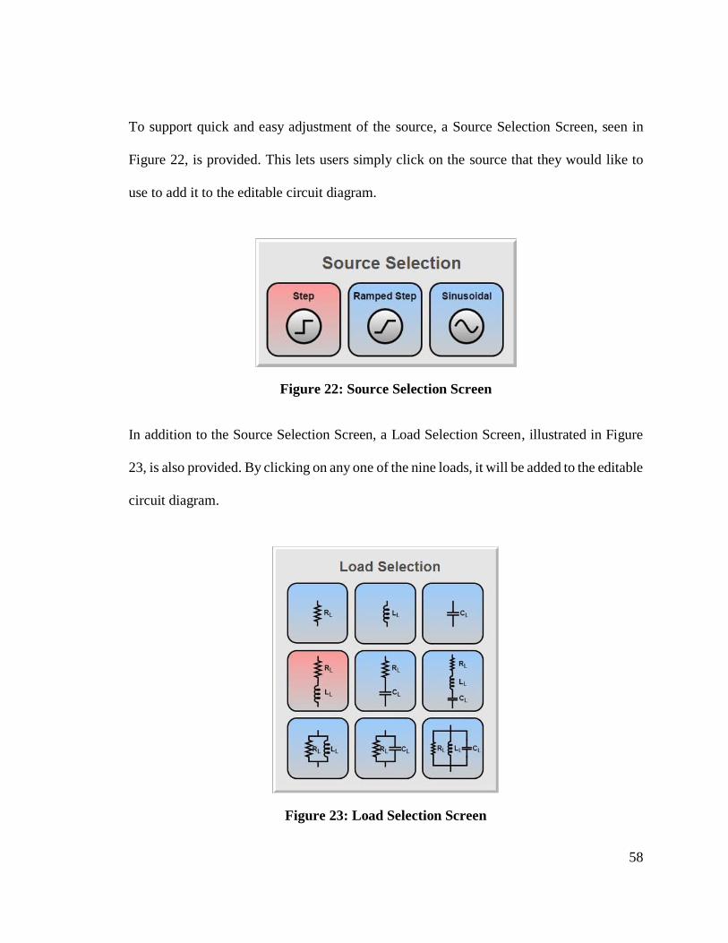
To support quick and easy adjustment of the source, a Source Selection Screen, seen in
Figure 22, is provided. This lets users simply click on the source that they would like to
use to add it to the editable circuit diagram.
Figure 22: Source Selection Screen
In addition to the Source Selection Screen, a Load Selection Screen, illustrated in Figure
23, is also provided. By clicking on any one of the nine loads, it will be added to the editable
circuit diagram.
Figure 23: Load Selection Screen
59
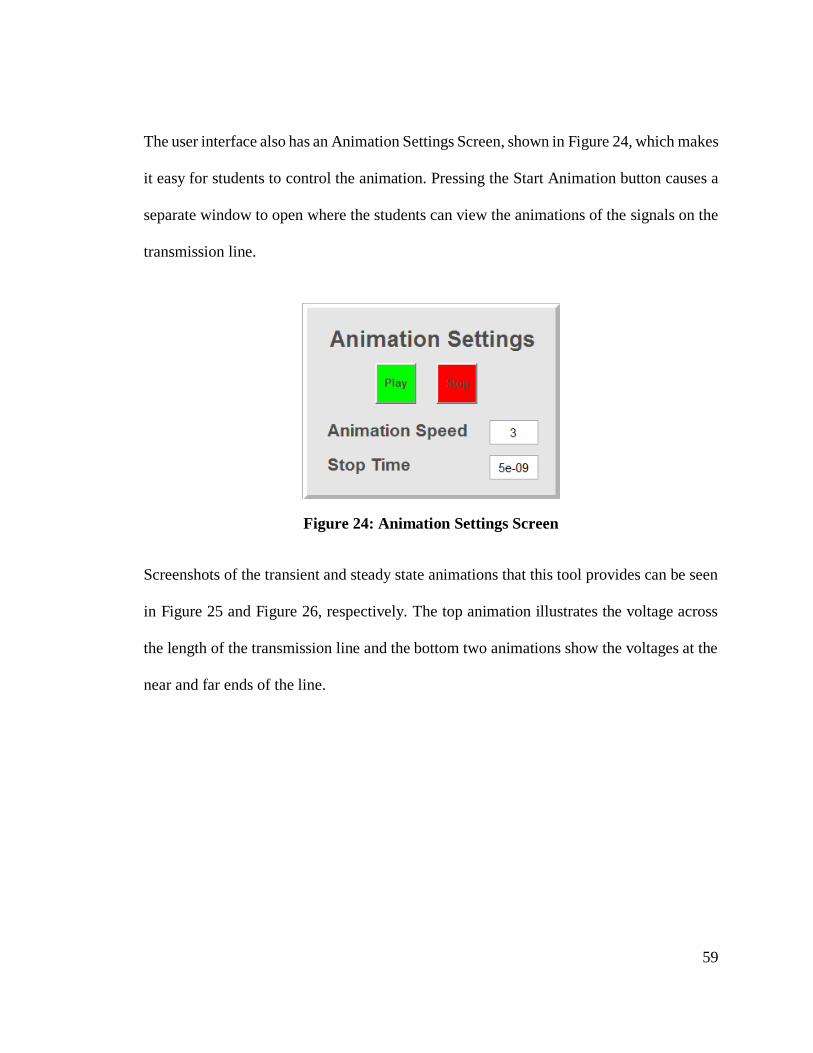
The user interface also has an Animation Settings Screen, shown in Figure 24, which makes
it easy for students to control the animation. Pressing the Start Animation button causes a
separate window to open where the students can view the animations of the signals on the
transmission line.
Figure 24: Animation Settings Screen
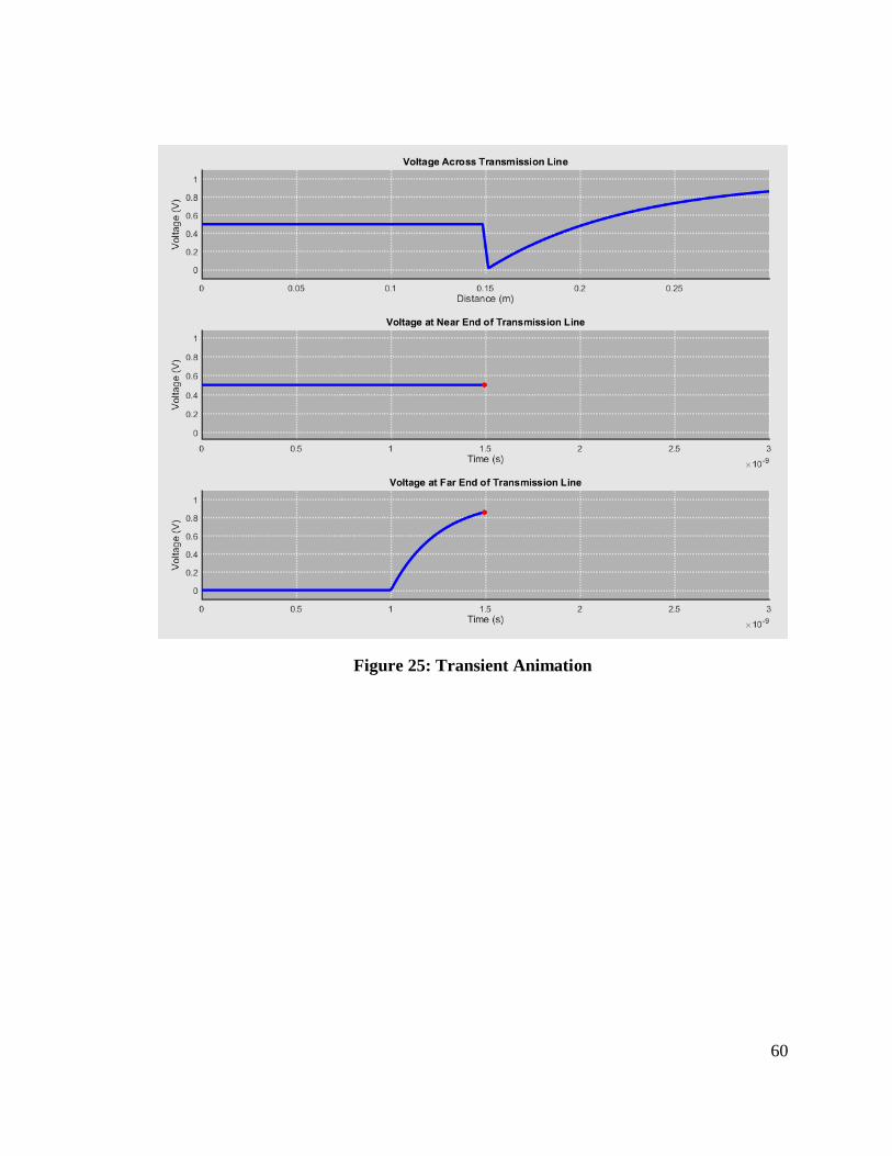
Screenshots of the transient and steady state animations that this tool provides can be seen
in Figure 25 and Figure 26, respectively. The top animation illustrates the voltage across
the length of the transmission line and the bottom two animations show the voltages at the
near and far ends of the line.
60
Figure 25: Transient Animation

61
Figure 26: Steady State Animation

62
4.3 Verification
A variety of methods are used to verify that the animations produced by this tool are
accurate. To verify the transient animations, two different approaches are used. The first
approach compares the signals at the near and far ends of the line with simulations in
LTspice. LTspice is a circuit simulator that is commonly used to model electrical circuits.
The second approach tests that the transient animations approach the expected steady state
value if the simulation is run for a relatively long time. To verify the steady state
animations, the standing wave patterns that are created by this tool are compared with
standing wave patterns that are generated by the online tool illustrated in Figure 8. All of
these tests are conducted using variety of circuit configurations. Additional details about
each test, as well as the test results are provided in the following section.
4.3.1 Transient Animation Verification
LTspice Transient Animation Verification
The LTspice comparisons of the signals at the near and far ends of the transmission line
are illustrated in the figures below. Two separate circuits were designed for each of the
three sources. The figures show the circuit that was built in this tool, the circuit that was
built in LTspice, and a picture that overlays the signals generated by this tool and by
LTspice on top of each other. The signals generated by this tool are shown in dark blue and
red. The signals that were generated by LTspice are shown in light blue and orange.
Additional verification plots are shown in Appendix E.

63
LTspice Transient Animation Verification – Step Circuit
Figure 27: Transient Animation Verification – Step Circuit (Tool)
Figure 28: Transient Animation Verification – Step Circuit (LTspice)

64
Figure 29: Transient Animation Verification – Step Circuit (Plots)

65
LTspice Transient Animation Verification – Ramped Step Circuit
Figure 30: Transient Animation Verification – Ramped Step Circuit (Tool)
Figure 31: Transient Animation Verification – Ramped Step Circuit (LTspice)

66
Figure 32: Transient Animation Verification – Ramped Step Circuit (Plots)

67
LTspice Transient Animation Verification – Sine Circuit
Figure 33: Transient Animation Verification – Sine Circuit (Tool)
Figure 34: Transient Animation Verification – Sine Circuit (LTspice)

68
Figure 35: Transient Animation Verification – Sine Circuit (Plots)

69
Transients Animations Approaching Steady State Verification
The figures illustrated below demonstrate that the transient animations approach the
expected steady state value when the simulation is run for a relatively long period of time.
A description of how the steady state values of the signals are calculated for each test is
also provided. Additional verification plots are shown in Appendix E.

70
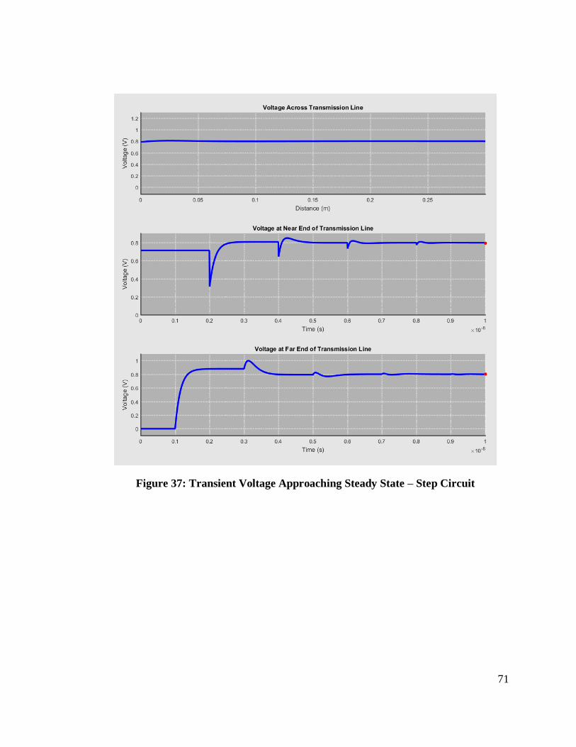
Transient Animations Approaching Steady State – Step and Ramped Step Circuits
At steady state, the capacitor shown in Figure 36 acts as an open circuit and the inductor
shown in Figure 39 acts as a short circuit. The steady state voltage can be calculated using
(75). The steady state current can be calculated using (76).
𝑣𝑠𝑠 = 𝑣𝑆(𝑡 = ∞) ·𝑅𝐿
𝑅𝑆 + 𝑅𝐿=80
100= 0.8 V (75)
𝑖𝑠𝑠 =𝑣𝑆(𝑡 = ∞)
𝑅𝑆 + 𝑅𝐿=
1
100= 10 mA (76)
Looking at Figure 37, Figure 38, Figure 40, and Figure 41, the voltages and currents across
the line and at the ends of the line are all approaching the expected steady state values.
Figure 36: Transient Animations Approaching Steady State – Step Circuit
71
Figure 37: Transient Voltage Approaching Steady State – Step Circuit

72
Figure 38: Transient Current Approaching Steady State – Step Circuit

73
Figure 39: Transient Animations Approaching Steady State – Ramped Step Circuit

74
Figure 40: Transient Voltage Approaching Steady State – Ramped Step Circuit

75
Figure 41: Transient Current Approaching Steady State – Ramped Step Circuit

76
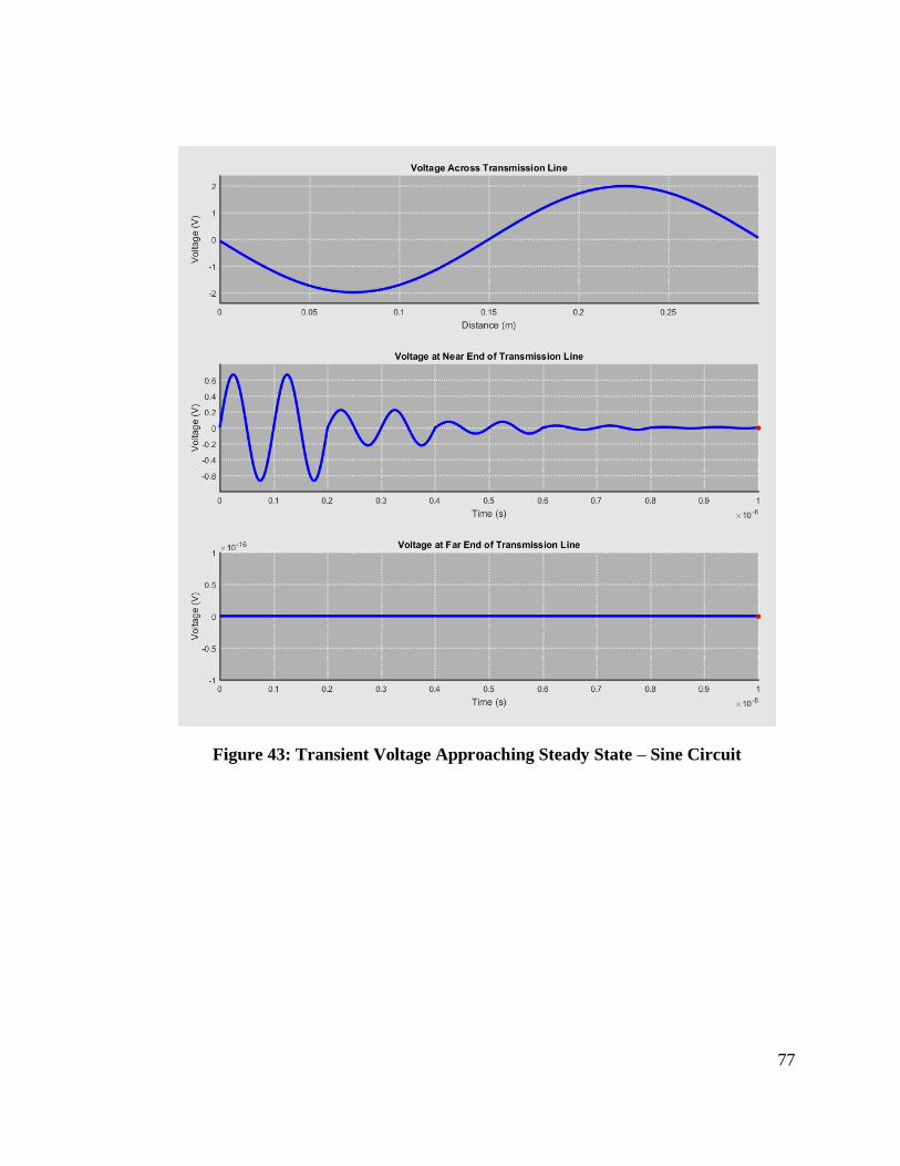
Transient Animations Approaching Steady State – Sine Circuit
Since the load shown in Figure 42 is shorted, a sinusoidal source is being used, and the
wave length of the signal is equal to the length of the line, the expected steady state voltage
can be calculated using (77). The steady state current can be calculated using (78).
𝑣𝑠𝑠(𝑧 = 0) = 𝑣𝑠𝑠(𝑧 = 𝑙) = 𝑣𝑆(𝑡 = ∞) ·𝑅𝐿
𝑅𝑆 + 𝑅𝐿= 0 · 𝑠𝑖𝑛(2𝜋𝑓𝑡) = 0 V (77)
𝑖𝑠𝑠(𝑧 = 0) = 𝑖𝑠𝑠(𝑧 = 𝑙) =𝑣𝑆(𝑡 = ∞)
𝑅𝑆 + 𝑅𝐿=1
25· 𝑠𝑖𝑛(2𝜋𝑓𝑡) = 40 · 𝑠𝑖𝑛 (2𝜋𝑓𝑡) mA (78)
Looking at Figure 43 and Figure 38, the voltages and currents at the ends of the line are all
approaching the expected steady state values.
Figure 42: Transient Animations Approaching Steady State – Sine Circuit
77
Figure 43: Transient Voltage Approaching Steady State – Sine Circuit

78
Figure 44: Transient Current Approaching Steady State – Sine Circuit

79
4.3.2 Steady State Animation Verification
To verify the accuracy of the steady state animations, three different circuits were created.
These circuits can be seen in Figure 45, Figure 60, and Figure 65. Each of these circuits
was also created in the online tool, which can be seen in Figure 46, Figure 61, and Figure
66. Once the circuits were created, standing wave patterns for the voltage and the current
across the line were generated by each of the tools. On each standing wave plot, two data
points are indicated to show that the standing wave patterns match for this tool and the
online tool. Take note that x-axis for this tool is 𝑧 = 0 at the near end and 𝑧 = 𝑙 at the far
end, while the x-axis of the online tool is 𝑧 = 𝑙 at the near end and 𝑧 = 0 at the far end.
Additional verification plots are shown in Appendix E.

80
Steady State Standing Wave Pattern Comparison
Figure 45: Steady State Verification (Tool)
Figure 46: Steady State Verification (Online Tool) [8]

81
Figure 47: Steady State Standing Wave Patterns Created by this Tool
Figure 48: Steady State Standing Wave Patterns Created by Online Tool (Case A)
[8]

82
Figure 49: Steady State Standing Wave Patterns Created by Online Tool (Case B)
[8]

83
5. Conclusion
To fully understand transmission lines, electrical engineers must be able to visualize the
signals across the line. Since these signals vary over both time and space, they can be
difficult to envisage using traditional methods. Two educators have created tools that
animate signals across transmission lines, but neither of these tools are capable of
illustrating:
1. Transient response of a transmission line with a transient sinusoidal source
2. Transient response of a transmission line with unmatched source impedance
The goal of this project was to implement an open source, interactive learning tool that will
help students explore fundamental transmission line concepts. By reiterating the important
topics covered by the previous tools and incorporating the unrepresented concepts, this tool
addresses the need for a comprehensive tool to teach transmission line concepts.

84
6. Future Work
This section will discuss additional work that could be completed to enhance the Interactive
Tool for Teaching Transmission Line Concepts.
6.1 Improvements on Current Tool
There are several features that could be added to the current tool to enhance its
functionality. A relatively easy improvement that could be made is providing students with
additional voltage sources. This would give them more opportunity to explore and gain
intuition about transmission lines. These sources could include a:
Pulse generator
Pulse train generator
Square wave generator
Sawtooth wave generator
Triangle wave generator
Another useful, but more challenging feature that could be added is providing transient
animations for lossy transmission lines. This could help students understand how loss on a
transmission line can affect signals shortly after the source has been turned on. One more
feature that could be added to this tool is giving students the option to place a stub
somewhere along the line. Having this capability while also being able to animate signals

85
on the line could help students gain insight into why stubs are used in various transmission
line applications.
6.2 User Testing and Feedback
Since one of the main objectives for this tool was for it to be approachable to beginning
students, the ease of use was an important factor. At this time, this tool has only been tested
by the developer. Giving students access to the tool and gathering their feedback would
reveal additional improvements to be made. Some of these improvements could include
refinements of the user interface or new animations to help students better understand
transmission lines.

86
Bibliography
[1] U. S. Inan and A. S. Inan, "Reflection at Discontinuities," in Engineering
Electromagnetics, Menlo Park, Addison-Wesley, 1999, pp. 34-37.
[2] P. Falstad, "Circuit Simulator Applet," Falstad.com, Inc., [Online]. Available:
http://www.falstad.com/circuit/. [Accessed 6 May 2017].
[3] "Amanogawa.com," [Online]. Available: http://www.amanogawa.com/index.html.
[Accessed 8 May 2017].
[4] P. Falstad, "Simple Transmission Lines," Falstad.com, Inc., 7 Dec 2016. [Online].
Available: http://www.falstad.com/circuit/e-tl.html. [Accessed 6 May 2017].
[5] P. Falstad, "Standing Wave on a Transmission Line," Falstad.com, Inc., 7 Dec 2016.
[Online]. Available: http://www.falstad.com/circuit/e-tlstand.html. [Accessed 6 May
2017].
[6] P. Falstad, "Termination of a Transmission Line," Falstad.com, Inc., 7 Dec 2016.
[Online]. Available: http://www.falstad.com/circuit/e-tlterm.html. [Accessed 6 May
2017].
[7] "Interactive Smith Chart General Lossy Line," Amanogawa, [Online]. Available:
http://www.amanogawa.com/archive/LossySmithChart/LossySmithChart-2.html.
[Accessed 7 May 2017].
[8] "General Lossy Line (wide plots)," Amanogawa, [Online]. Available:
http://www.amanogawa.com/archive/LossyWide/LossyWide-2.html. [Accessed 7
May 2017].
[9] "Transient Line with Capacitive Load," Amanogawa, [Online]. Available:
http://www.amanogawa.com/archive/ShuntCapacitance/ShuntCapacitance-2.html.
[Accessed 7 May 2017].
[10] "Table of Laplace Transforms," [Online]. Available:
http://tutorial.math.lamar.edu//pdf/Laplace_Table.pdf. [Accessed 17 May 2017].
[11] U. S. Inan and A. S. Inan, "Sinusoidal Steady-State Behavior of Lossy Lines," in
Engineering Electromagnetics, Menlo Park, Addison-Wesley, 1999, pp. 199-216.

87
[12] P. C. Magnusson, G. C. Alexander, V. K. Tripathi and A. Weisshaar, "Wave
Distortion on Lossy Lines — Step-Function Source," in Transmission Lines and
Wave Propagation 4th Edition, Boca Raton, CRC Press, 2001, pp. 76-80.
[13] P. C. Magnusson, G. C. Alexander, V. K. Tripathi and A. Weisshaar, "Wave
Propagation on an Infinite Lossless Line," in Transmission Lines and Wave
Propagation 4th Edition, Boca Raton, CRC Press, 2001, pp. 11-24.
[14] S. D. S. John W. Lee, "Geometric Series," in Matrix and Power Series Methods Fifth
Edition, Hoboken, Wiley, 2013, p. 135.
[15] B. M. Notaros, "Complex Representatives of Time-Harmonic Field and Circuit
Quantities," in MATLAB-Based Electromagnetics, Boston, Pearson, 2014, p. 138.
[16] E. Cheever, "Table of Laplace Transform Properties," Swarthmore College, 2015.
[Online]. Available:
http://lpsa.swarthmore.edu/LaplaceZTable/LaplacePropTable.html. [Accessed 4
June 2017].

88
Appendices
Appendix A: Ramped Step Laplace Transform Derivation
Appendix B: Generating Animation Data for the Signals Across the Line
Appendix C: Generating Animations for the Signals Across the Line
Appendix D: Generating Animations for Signals at the Ends of the Line
Appendix E: Additional Verification Examples
Appendix F: Download the Interactive Tool for Teaching Transmission Line Concepts
Appendix G: Common Development and Distribution License

89
Appendix A: Ramped Step Laplace Transform Derivation
The Laplace transform of the ramped step function is derived in this section. The ramped
step function is created by subtracting a line with slope 𝐴
𝑡𝑟 that starts at the origin from a
line with the same slope that is offset by 𝑡𝑟, where 𝐴 is the amplitude of the ramped step
and 𝑡𝑟 is the rise time of the ramped step. Figure 50 illustrates how the ramped step function
is created.
Figure 50: Creating the Ramped Step Function
(80) is the time domain formula for calculating the ramped step function, where 𝑢(𝑡)
represents the unit step function.
𝑣(𝑡) = 𝐴
𝑡𝑟· 𝑡 · 𝑢(𝑡) −
𝐴
𝑡𝑟· (𝑡 − 𝑡𝑟) · 𝑢(𝑡 − 𝑡𝑟) (79)
Using a table of Laplace transforms [10], the Laplace transform of a line with a slope of 1
is illustrated in (80).

90
𝑡 ℒ⇔
1
𝑠2 (80)
Using the linearity property of the Laplace transform [16], a line with slope 𝐴
𝑡𝑟 can be
generated by multiplying (80) by 𝐴
𝑡𝑟, resulting in (81).
𝐴
𝑡𝑟· 𝑡
ℒ⇔
𝐴
𝑡𝑟·1
𝑠2 (81)
To shift a function, 𝑓(𝑡), in time, the time shift property of the Laplace transform, shown
in (82), can be used. Along with shifting 𝑓(𝑡) in time, this property also multiples the
shifted function by a shifted unit step function.
𝑓(𝑡 − 𝑡0) · 𝑢(𝑡 − 𝑡0) ℒ⇔ 𝑒−𝑡0·𝑠 · 𝐹(𝑠) (82)
Using the time shift property shown in (82) along with the formula for creating a line with
slope 𝐴
𝑡𝑟 that was developed in (81), the general equation for the Laplace transform of a
ramped step with amplitude 𝐴 and rise time 𝑡𝑟 can be calculated, as illustrated in .
𝑣(𝑡) = 𝐴
𝑡𝑟· [𝑡 · 𝑢(𝑡) − (𝑡 − 𝑡𝑟) · 𝑢(𝑡 − 𝑡𝑟)]
ℒ⇔ 𝑉(𝑠) =
𝐴
𝑡𝑟·1
𝑠2· [1 − 𝑒−𝑡𝑟·𝑠] (83)
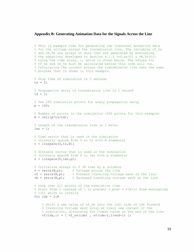
91
Appendix B: Generating Animation Data for the Signals Across the Line
% This is example code for generating the transient animation data % for the voltage across the transmission line. The variables vf_ne % and vb_fe are arrays of data that are generated by evaluating % the equations developed in Section 4.1.3 (vf,ne(t) & vb,fe(t)) % using the time array, t, which is shown below. The values for % vf_ne and vb_fe must be calculated before this code will run. % Calculating the current across the transmission line uses the same % process that is shown in this example.
% Stop time of simulation is 5 seconds ts = 5;
% Propagation delay of transmission line is 1 second td = 1;
% Use 100 simulation points for every propagation delay p = 100;
% Number of points in the simulation (500 points for this example) N = ceil(p*ts/td);
% Length of the transmission line is 1 meter len = 1;
% Time vector that is used in the simulation % (Linearly spaced from 0 to ts with N elements) t = linspace(0,ts,N);
% Distance vector that is used in the simulation % (Linearly spaced from 0 to len with p elements) z = linspace(0,len,p);
% Initialize arrays to 0 (N rows by p columns) v = zeros(N,p); % Voltage across the line vf = zeros(N,p); % Forward traveling voltage wave on the line vb = zeros(N,p); % Backward traveling voltage wave on the line
% Loop over all points of the simulation time % Start from 2 instead of 1 to prevent t_prev = t(k-1) from evaluating % t(0) which is invalid for idx = 2:N
% Shift a new value of vf_ne into the left side of the forward % traveling voltage wave array at every new instant of the % simulation, discarding the oldest value at the end of the line vf(idx,:) = [ vf_ne(idx) , vf(idx-1,1:end-1) ];

92
% Shift a new value of vb_fe into the right side of the backward % traveling voltage wave array at every new instant of the % simulation, discarding the oldest value at the end of the line vb(idx,:) = [vb(idx-1,2:end),vb_fe(idx)];
% The sum of the forward and backward traveling voltage waves on % the transmission line is the overall voltage across the line. v(idx,:) = vf(idx,:) + vb(idx,:);
end

93
Appendix C: Generating Animations for the Signals Across the Line
% This is example code for generating an animation of a signal across % the transmission line. A generic variable called sig is used to % represent the animation data. The format of this animation data is % described in Section 4.2.2. An example signal has been created that % will allow the animation to run. This signal is purely for % demonstration purposes and was not modeled after a transmission % line.
% Stop time of simulation is 5 seconds ts = 5;
% Propagation delay of transmission line is 1 second td = 1;
% Use 100 simulation points for every propagation delay p = 100;
% Number of points in the simulation (500 points for this example) N = ceil(p*ts/td);
% Length of the transmission line is 1 meter len = 1;
% Time vector that is used in the simulation % (Linearly spaced from 0 to ts with N elements) t = linspace(0,ts,N)';
% Distance vector that is used in the simulation % (Linearly spaced from 0 to len with p elements) z = linspace(0,len,p);
% This is a generic signal that is created to let the code run sig = sin(pi*t)*sin(2*pi*z);
% Speed of the animation % (must be an integer greater than or equal to 1) speed = 2;
% Loop from the first point in the simulation to the last point in the % simulation, incrementing by speed, which is 2 in this example for time_idx = 1:speed:N
% Plot the signal across the line for the instant in time % specified by time_idx plot( z, sig(time_idx,:) );

94
% Set the x axis limits % (from 0 meters to len) xlim([0 len]);
% Set the y axis limits % (from the smallest value of sig to the largest value of sig) ylim([min(min(sig)), max(max(sig))]);
% This limits the frame rate of the animation to 20 frames per sec drawnow;
end

95
Appendix D: Generating Animations for Signals at the Ends of the Line
% This is example code for generating an animation of a signal at % either end of the line. A generic variable called sig is used to % represent the animation data. The format of this animation data is % described in Section 4.2.2. An example signal has been created that % will allow the animation to run. This signal is purely for % demonstration purposes and was not modeled after a transmission % line.
% Stop time of simulation is 5 seconds ts = 5;
% Propagation delay of transmission line is 1 second td = 1;
% Use 100 simulation points for every propagation delay p = 100;
% Number of points in the simulation (500 points for this example) N = ceil(p*ts/td);
% Time vector that is used in the simulation % (Linearly spaced from 0 to ts with N elements) t = linspace(0,ts,N)';
% This is a generic signal that is created to let the code run sig = sin(2*pi*t);
% Speed of the animation % (must be an integer greater than or equal to 1) speed = 2;
% Loop from the first point in the simulation to the last point in the % simulation, incrementing by speed, which is 2 in this example for time_idx = 1:speed:N
% Plot the signal at the end of the line, adding new points to the % plot every iteration of the loop plot( t(1:time_idx), sig(1:time_idx) );
% Set the x axis limits % (from 0 seconds to ts) xlim([0 ts]);
% Set the y axis limits % (from the smallest value of sig to the largest value of sig) ylim([min(sig), max(sig)]);

96
% This limits the frame rate of the animation to 20 frames per sec drawnow;
end

97
Appendix E: Additional Verification Data
This section provides additional verification of the accuracy of this tool. Explanations of
these images can be seen in Section 4.3.
LTspice Transient Animation Verification – Step Circuit 2
Figure 51: Transient Animation Verification – Step Circuit 2 (Tool)
Figure 52: Transient Animation Verification – Step Circuit 2 (LTspice)

98
Figure 53: Transient Animation Verification – Step Circuit 2 (Plots)

99
LTspice Transient Animation Verification – Ramped Step Circuit 2
Figure 54: Transient Animation Verification – Ramped Step Circuit 2 (Tool)
Figure 55: Transient Animation Verification – Ramped Step Circuit 2 (LTspice)

100
Figure 56: Transient Animation Verification – Ramped Step Circuit 2 (Plots)

101
LTspice Transient Animation Verification – Sine Circuit 2
Figure 57: Transient Animation Verification – Sine Circuit 2 (Tool)
Figure 58: Transient Animation Verification – Sine Circuit 2 (LTspice)

102
Figure 59: Transient Animation Verification – Sine Circuit 2 (Plots)

103
Steady State Standing Wave Pattern Comparison – Circuit 2
Figure 60: Steady State Verification – Circuit 2 (Tool)
Figure 61: Steady State Verification – Circuit 2 (Online Tool) [8]

104
Figure 62: Steady State Standing Wave Patterns Created by this Tool – Circuit 2
Figure 63: Steady State Standing Wave Patterns Created by Online Tool (Case A) –
Circuit 2 [8]
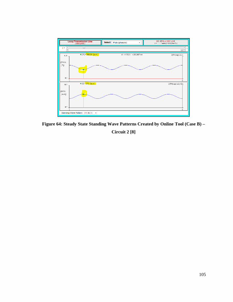
105
Figure 64: Steady State Standing Wave Patterns Created by Online Tool (Case B) –
Circuit 2 [8]
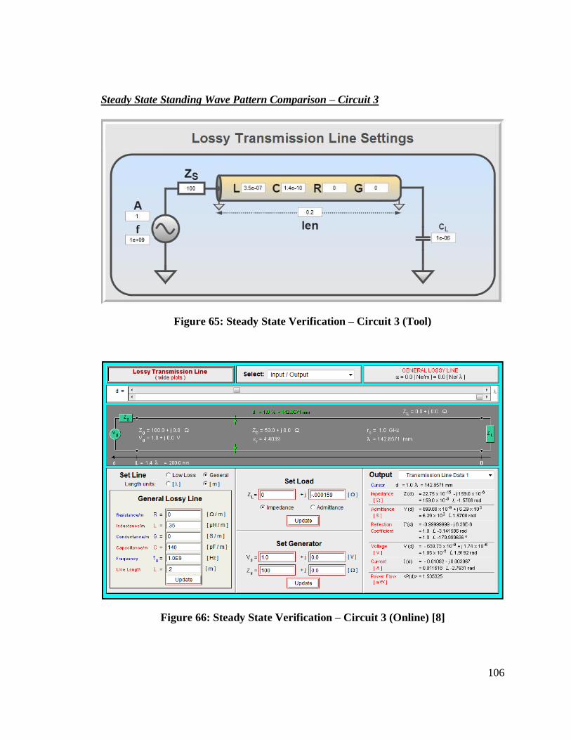
106
Steady State Standing Wave Pattern Comparison – Circuit 3
Figure 65: Steady State Verification – Circuit 3 (Tool)
Figure 66: Steady State Verification – Circuit 3 (Online) [8]

107
Figure 67: Steady State Standing Wave Patterns Created by this Tool – Circuit 3
Figure 68: Steady State Standing Wave Patterns Created by Online Tool (Case A) –
Circuit 3 [8]

108
Figure 69: Steady State Standing Wave Patterns Created by Online Tool (Case B) –
Circuit 3 [8]

109
Appendix F: Download the Interactive Tool for Teaching Transmission Line Concepts
The Interactive Tool for Teaching Transmission Line Concepts is licensed under the
GNU General Public License v3.0, and is available for free at:
https://github.com/keatoncscheible/Transmission_Lines_Simulation

110
Appendix G: Common Development and Distribution License
GNU GENERAL PUBLIC LICENSE Version 3, 29 June 2007 Copyright (C) 2007 Free Software Foundation, Inc. <http://fsf.org/> Everyone is permitted to copy and distribute verbatim copies of this license document, but changing it is not allowed. Preamble The GNU General Public License is a free, copyleft license for software and other kinds of works. The licenses for most software and other practical works are designed to take away your freedom to share and change the works. By contrast, the GNU General Public License is intended to guarantee your freedom to share and change all versions of a program--to make sure it remains free software for all its users. We, the Free Software Foundation, use the GNU General Public License for most of our software; it applies also to any other work released this way by its authors. You can apply it to your programs, too. When we speak of free software, we are referring to freedom, not price. Our General Public Licenses are designed to make sure that you have the freedom to distribute copies of free software (and charge for them if you wish), that you receive source code or can get it if you want it, that you can change the software or use pieces of it in new free programs, and that you know you can do these things. To protect your rights, we need to prevent others from denying you these rights or asking you to surrender the rights. Therefore, you have certain responsibilities if you distribute copies of the software, or if you modify it: responsibilities to respect the freedom of others. For example, if you distribute copies of such a program, whether gratis or for a fee, you must pass on to the recipients the same freedoms that you received. You must make sure that they, too, receive or can get the source code. And you must show them these terms so they know their rights. Developers that use the GNU GPL protect your rights with two steps: (1) assert copyright on the software, and (2) offer you this License giving you legal permission to copy, distribute and/or modify it. For the developers' and authors' protection, the GPL clearly explains

111
that there is no warranty for this free software. For both users' and authors' sake, the GPL requires that modified versions be marked as changed, so that their problems will not be attributed erroneously to authors of previous versions. Some devices are designed to deny users access to install or run modified versions of the software inside them, although the manufacturer can do so. This is fundamentally incompatible with the aim of protecting users' freedom to change the software. The systematic pattern of such abuse occurs in the area of products for individuals to use, which is precisely where it is most unacceptable. Therefore, we have designed this version of the GPL to prohibit the practice for those products. If such problems arise substantially in other domains, we stand ready to extend this provision to those domains in future versions of the GPL, as needed to protect the freedom of users. Finally, every program is threatened constantly by software patents. States should not allow patents to restrict development and use of software on general-purpose computers, but in those that do, we wish to avoid the special danger that patents applied to a free program could make it effectively proprietary. To prevent this, the GPL assures that patents cannot be used to render the program non-free. The precise terms and conditions for copying, distribution and modification follow. TERMS AND CONDITIONS 0. Definitions. "This License" refers to version 3 of the GNU General Public License. "Copyright" also means copyright-like laws that apply to other kinds of works, such as semiconductor masks. "The Program" refers to any copyrightable work licensed under this License. Each licensee is addressed as "you". "Licensees" and "recipients" may be individuals or organizations. To "modify" a work means to copy from or adapt all or part of the work in a fashion requiring copyright permission, other than the making of an exact copy. The resulting work is called a "modified version" of the earlier work or a work "based on" the earlier work. A "covered work" means either the unmodified Program or a work based on the Program. To "propagate" a work means to do anything with it that, without

112
permission, would make you directly or secondarily liable for infringement under applicable copyright law, except executing it on a computer or modifying a private copy. Propagation includes copying, distribution (with or without modification), making available to the public, and in some countries other activities as well. To "convey" a work means any kind of propagation that enables other parties to make or receive copies. Mere interaction with a user through a computer network, with no transfer of a copy, is not conveying. An interactive user interface displays "Appropriate Legal Notices" to the extent that it includes a convenient and prominently visible feature that (1) displays an appropriate copyright notice, and (2) tells the user that there is no warranty for the work (except to the extent that warranties are provided), that licensees may convey the work under this License, and how to view a copy of this License. If the interface presents a list of user commands or options, such as a menu, a prominent item in the list meets this criterion. 1. Source Code. The "source code" for a work means the preferred form of the work for making modifications to it. "Object code" means any non-source form of a work. A "Standard Interface" means an interface that either is an official standard defined by a recognized standards body, or, in the case of interfaces specified for a particular programming language, one that is widely used among developers working in that language. The "System Libraries" of an executable work include anything, other than the work as a whole, that (a) is included in the normal form of packaging a Major Component, but which is not part of that Major Component, and (b) serves only to enable use of the work with that Major Component, or to implement a Standard Interface for which an implementation is available to the public in source code form. A "Major Component", in this context, means a major essential component (kernel, window system, and so on) of the specific operating system (if any) on which the executable work runs, or a compiler used to produce the work, or an object code interpreter used to run it. The "Corresponding Source" for a work in object code form means all the source code needed to generate, install, and (for an executable work) run the object code and to modify the work, including scripts to control those activities. However, it does not include the work's System Libraries, or general-purpose tools or generally available free programs which are used unmodified in performing those activities but which are not part of the work. For example, Corresponding Source

113
includes interface definition files associated with source files for the work, and the source code for shared libraries and dynamically linked subprograms that the work is specifically designed to require, such as by intimate data communication or control flow between those subprograms and other parts of the work. The Corresponding Source need not include anything that users can regenerate automatically from other parts of the Corresponding Source. The Corresponding Source for a work in source code form is that same work. 2. Basic Permissions. All rights granted under this License are granted for the term of copyright on the Program, and are irrevocable provided the stated conditions are met. This License explicitly affirms your unlimited permission to run the unmodified Program. The output from running a covered work is covered by this License only if the output, given its content, constitutes a covered work. This License acknowledges your rights of fair use or other equivalent, as provided by copyright law. You may make, run and propagate covered works that you do not convey, without conditions so long as your license otherwise remains in force. You may convey covered works to others for the sole purpose of having them make modifications exclusively for you, or provide you with facilities for running those works, provided that you comply with the terms of this License in conveying all material for which you do not control copyright. Those thus making or running the covered works for you must do so exclusively on your behalf, under your direction and control, on terms that prohibit them from making any copies of your copyrighted material outside their relationship with you. Conveying under any other circumstances is permitted solely under the conditions stated below. Sublicensing is not allowed; section 10 makes it unnecessary. 3. Protecting Users' Legal Rights From Anti-Circumvention Law. No covered work shall be deemed part of an effective technological measure under any applicable law fulfilling obligations under article 11 of the WIPO copyright treaty adopted on 20 December 1996, or similar laws prohibiting or restricting circumvention of such measures. When you convey a covered work, you waive any legal power to forbid circumvention of technological measures to the extent such circumvention

114
is effected by exercising rights under this License with respect to the covered work, and you disclaim any intention to limit operation or modification of the work as a means of enforcing, against the work's users, your or third parties' legal rights to forbid circumvention of technological measures. 4. Conveying Verbatim Copies. You may convey verbatim copies of the Program's source code as you receive it, in any medium, provided that you conspicuously and appropriately publish on each copy an appropriate copyright notice; keep intact all notices stating that this License and any non-permissive terms added in accord with section 7 apply to the code; keep intact all notices of the absence of any warranty; and give all recipients a copy of this License along with the Program. You may charge any price or no price for each copy that you convey, and you may offer support or warranty protection for a fee. 5. Conveying Modified Source Versions. You may convey a work based on the Program, or the modifications to produce it from the Program, in the form of source code under the terms of section 4, provided that you also meet all of these conditions: a) The work must carry prominent notices stating that you modified it, and giving a relevant date. b) The work must carry prominent notices stating that it is released under this License and any conditions added under section 7. This requirement modifies the requirement in section 4 to "keep intact all notices". c) You must license the entire work, as a whole, under this License to anyone who comes into possession of a copy. This License will therefore apply, along with any applicable section 7 additional terms, to the whole of the work, and all its parts, regardless of how they are packaged. This License gives no permission to license the work in any other way, but it does not invalidate such permission if you have separately received it. d) If the work has interactive user interfaces, each must display Appropriate Legal Notices; however, if the Program has interactive interfaces that do not display Appropriate Legal Notices, your work need not make them do so. A compilation of a covered work with other separate and independent works, which are not by their nature extensions of the covered work,

115
and which are not combined with it such as to form a larger program, in or on a volume of a storage or distribution medium, is called an "aggregate" if the compilation and its resulting copyright are not used to limit the access or legal rights of the compilation's users beyond what the individual works permit. Inclusion of a covered work in an aggregate does not cause this License to apply to the other parts of the aggregate. 6. Conveying Non-Source Forms. You may convey a covered work in object code form under the terms of sections 4 and 5, provided that you also convey the machine-readable Corresponding Source under the terms of this License, in one of these ways: a) Convey the object code in, or embodied in, a physical product (including a physical distribution medium), accompanied by the Corresponding Source fixed on a durable physical medium customarily used for software interchange. b) Convey the object code in, or embodied in, a physical product (including a physical distribution medium), accompanied by a written offer, valid for at least three years and valid for as long as you offer spare parts or customer support for that product model, to give anyone who possesses the object code either (1) a copy of the Corresponding Source for all the software in the product that is covered by this License, on a durable physical medium customarily used for software interchange, for a price no more than your reasonable cost of physically performing this conveying of source, or (2) access to copy the Corresponding Source from a network server at no charge. c) Convey individual copies of the object code with a copy of the written offer to provide the Corresponding Source. This alternative is allowed only occasionally and noncommercially, and only if you received the object code with such an offer, in accord with subsection 6b. d) Convey the object code by offering access from a designated place (gratis or for a charge), and offer equivalent access to the Corresponding Source in the same way through the same place at no further charge. You need not require recipients to copy the Corresponding Source along with the object code. If the place to copy the object code is a network server, the Corresponding Source may be on a different server (operated by you or a third party) that supports equivalent copying facilities, provided you maintain clear directions next to the object code saying where to find the Corresponding Source. Regardless of what server hosts the

116
Corresponding Source, you remain obligated to ensure that it is available for as long as needed to satisfy these requirements. e) Convey the object code using peer-to-peer transmission, provided you inform other peers where the object code and Corresponding Source of the work are being offered to the general public at no charge under subsection 6d. A separable portion of the object code, whose source code is excluded from the Corresponding Source as a System Library, need not be included in conveying the object code work. A "User Product" is either (1) a "consumer product", which means any tangible personal property which is normally used for personal, family, or household purposes, or (2) anything designed or sold for incorporation into a dwelling. In determining whether a product is a consumer product, doubtful cases shall be resolved in favor of coverage. For a particular product received by a particular user, "normally used" refers to a typical or common use of that class of product, regardless of the status of the particular user or of the way in which the particular user actually uses, or expects or is expected to use, the product. A product is a consumer product regardless of whether the product has substantial commercial, industrial or non-consumer uses, unless such uses represent the only significant mode of use of the product. "Installation Information" for a User Product means any methods, procedures, authorization keys, or other information required to install and execute modified versions of a covered work in that User Product from a modified version of its Corresponding Source. The information must suffice to ensure that the continued functioning of the modified object code is in no case prevented or interfered with solely because modification has been made. If you convey an object code work under this section in, or with, or specifically for use in, a User Product, and the conveying occurs as part of a transaction in which the right of possession and use of the User Product is transferred to the recipient in perpetuity or for a fixed term (regardless of how the transaction is characterized), the Corresponding Source conveyed under this section must be accompanied by the Installation Information. But this requirement does not apply if neither you nor any third party retains the ability to install modified object code on the User Product (for example, the work has been installed in ROM). The requirement to provide Installation Information does not include a requirement to continue to provide support service, warranty, or updates for a work that has been modified or installed by the recipient, or for the User Product in which it has been modified or installed. Access to a

117
network may be denied when the modification itself materially and adversely affects the operation of the network or violates the rules and protocols for communication across the network. Corresponding Source conveyed, and Installation Information provided, in accord with this section must be in a format that is publicly documented (and with an implementation available to the public in source code form), and must require no special password or key for unpacking, reading or copying. 7. Additional Terms. "Additional permissions" are terms that supplement the terms of this License by making exceptions from one or more of its conditions. Additional permissions that are applicable to the entire Program shall be treated as though they were included in this License, to the extent that they are valid under applicable law. If additional permissions apply only to part of the Program, that part may be used separately under those permissions, but the entire Program remains governed by this License without regard to the additional permissions. When you convey a copy of a covered work, you may at your option remove any additional permissions from that copy, or from any part of it. (Additional permissions may be written to require their own removal in certain cases when you modify the work.) You may place additional permissions on material, added by you to a covered work, for which you have or can give appropriate copyright permission. Notwithstanding any other provision of this License, for material you add to a covered work, you may (if authorized by the copyright holders of that material) supplement the terms of this License with terms: a) Disclaiming warranty or limiting liability differently from the terms of sections 15 and 16 of this License; or b) Requiring preservation of specified reasonable legal notices or author attributions in that material or in the Appropriate Legal Notices displayed by works containing it; or c) Prohibiting misrepresentation of the origin of that material, or requiring that modified versions of such material be marked in reasonable ways as different from the original version; or d) Limiting the use for publicity purposes of names of licensors or authors of the material; or e) Declining to grant rights under trademark law for use of some trade names, trademarks, or service marks; or
118
f) Requiring indemnification of licensors and authors of that material by anyone who conveys the material (or modified versions of it) with contractual assumptions of liability to the recipient, for any liability that these contractual assumptions directly impose on those licensors and authors. All other non-permissive additional terms are considered "further restrictions" within the meaning of section 10. If the Program as you received it, or any part of it, contains a notice stating that it is governed by this License along with a term that is a further restriction, you may remove that term. If a license document contains a further restriction but permits relicensing or conveying under this License, you may add to a covered work material governed by the terms of that license document, provided that the further restriction does not survive such relicensing or conveying. If you add terms to a covered work in accord with this section, you must place, in the relevant source files, a statement of the additional terms that apply to those files, or a notice indicating where to find the applicable terms. Additional terms, permissive or non-permissive, may be stated in the form of a separately written license, or stated as exceptions; the above requirements apply either way. 8. Termination. You may not propagate or modify a covered work except as expressly provided under this License. Any attempt otherwise to propagate or modify it is void, and will automatically terminate your rights under this License (including any patent licenses granted under the third paragraph of section 11). However, if you cease all violation of this License, then your license from a particular copyright holder is reinstated (a) provisionally, unless and until the copyright holder explicitly and finally terminates your license, and (b) permanently, if the copyright holder fails to notify you of the violation by some reasonable means prior to 60 days after the cessation. Moreover, your license from a particular copyright holder is reinstated permanently if the copyright holder notifies you of the violation by some reasonable means, this is the first time you have received notice of violation of this License (for any work) from that copyright holder, and you cure the violation prior to 30 days after your receipt of the notice.

119
Termination of your rights under this section does not terminate the licenses of parties who have received copies or rights from you under this License. If your rights have been terminated and not permanently reinstated, you do not qualify to receive new licenses for the same material under section 10. 9. Acceptance Not Required for Having Copies. You are not required to accept this License in order to receive or run a copy of the Program. Ancillary propagation of a covered work occurring solely as a consequence of using peer-to-peer transmission to receive a copy likewise does not require acceptance. However, nothing other than this License grants you permission to propagate or modify any covered work. These actions infringe copyright if you do not accept this License. Therefore, by modifying or propagating a covered work, you indicate your acceptance of this License to do so. 10. Automatic Licensing of Downstream Recipients. Each time you convey a covered work, the recipient automatically receives a license from the original licensors, to run, modify and propagate that work, subject to this License. You are not responsible for enforcing compliance by third parties with this License. An "entity transaction" is a transaction transferring control of an organization, or substantially all assets of one, or subdividing an organization, or merging organizations. If propagation of a covered work results from an entity transaction, each party to that transaction who receives a copy of the work also receives whatever licenses to the work the party's predecessor in interest had or could give under the previous paragraph, plus a right to possession of the Corresponding Source of the work from the predecessor in interest, if the predecessor has it or can get it with reasonable efforts. You may not impose any further restrictions on the exercise of the rights granted or affirmed under this License. For example, you may not impose a license fee, royalty, or other charge for exercise of rights granted under this License, and you may not initiate litigation (including a cross-claim or counterclaim in a lawsuit) alleging that any patent claim is infringed by making, using, selling, offering for sale, or importing the Program or any portion of it. 11. Patents. A "contributor" is a copyright holder who authorizes use under this License of the Program or a work on which the Program is based. The work thus licensed is called the contributor's "contributor version".

120
A contributor's "essential patent claims" are all patent claims owned or controlled by the contributor, whether already acquired or hereafter acquired, that would be infringed by some manner, permitted by this License, of making, using, or selling its contributor version, but do not include claims that would be infringed only as a consequence of further modification of the contributor version. For purposes of this definition, "control" includes the right to grant patent sublicenses in a manner consistent with the requirements of this License. Each contributor grants you a non-exclusive, worldwide, royalty-free patent license under the contributor's essential patent claims, to make, use, sell, offer for sale, import and otherwise run, modify and propagate the contents of its contributor version. In the following three paragraphs, a "patent license" is any express agreement or commitment, however denominated, not to enforce a patent (such as an express permission to practice a patent or covenant not to sue for patent infringement). To "grant" such a patent license to a party means to make such an agreement or commitment not to enforce a patent against the party. If you convey a covered work, knowingly relying on a patent license, and the Corresponding Source of the work is not available for anyone to copy, free of charge and under the terms of this License, through a publicly available network server or other readily accessible means, then you must either (1) cause the Corresponding Source to be so available, or (2) arrange to deprive yourself of the benefit of the patent license for this particular work, or (3) arrange, in a manner consistent with the requirements of this License, to extend the patent license to downstream recipients. "Knowingly relying" means you have actual knowledge that, but for the patent license, your conveying the covered work in a country, or your recipient's use of the covered work in a country, would infringe one or more identifiable patents in that country that you have reason to believe are valid. If, pursuant to or in connection with a single transaction or arrangement, you convey, or propagate by procuring conveyance of, a covered work, and grant a patent license to some of the parties receiving the covered work authorizing them to use, propagate, modify or convey a specific copy of the covered work, then the patent license you grant is automatically extended to all recipients of the covered work and works based on it. A patent license is "discriminatory" if it does not include within the scope of its coverage, prohibits the exercise of, or is conditioned on the non-exercise of one or more of the rights that are specifically granted under this License. You may not convey a covered

121
work if you are a party to an arrangement with a third party that is in the business of distributing software, under which you make payment to the third party based on the extent of your activity of conveying the work, and under which the third party grants, to any of the parties who would receive the covered work from you, a discriminatory patent license (a) in connection with copies of the covered work conveyed by you (or copies made from those copies), or (b) primarily for and in connection with specific products or compilations that contain the covered work, unless you entered into that arrangement, or that patent license was granted, prior to 28 March 2007. Nothing in this License shall be construed as excluding or limiting any implied license or other defenses to infringement that may otherwise be available to you under applicable patent law. 12. No Surrender of Others' Freedom. If conditions are imposed on you (whether by court order, agreement or otherwise) that contradict the conditions of this License, they do not excuse you from the conditions of this License. If you cannot convey a covered work so as to satisfy simultaneously your obligations under this License and any other pertinent obligations, then as a consequence you may not convey it at all. For example, if you agree to terms that obligate you to collect a royalty for further conveying from those to whom you convey the Program, the only way you could satisfy both those terms and this License would be to refrain entirely from conveying the Program. 13. Use with the GNU Affero General Public License. Notwithstanding any other provision of this License, you have permission to link or combine any covered work with a work licensed under version 3 of the GNU Affero General Public License into a single combined work, and to convey the resulting work. The terms of this License will continue to apply to the part which is the covered work, but the special requirements of the GNU Affero General Public License, section 13, concerning interaction through a network will apply to the combination as such. 14. Revised Versions of this License. The Free Software Foundation may publish revised and/or new versions of the GNU General Public License from time to time. Such new versions will be similar in spirit to the present version, but may differ in detail to address new problems or concerns. Each version is given a distinguishing version number. If the Program specifies that a certain numbered version of the GNU General
122
Public License "or any later version" applies to it, you have the option of following the terms and conditions either of that numbered version or of any later version published by the Free Software Foundation. If the Program does not specify a version number of the GNU General Public License, you may choose any version ever published by the Free Software Foundation. If the Program specifies that a proxy can decide which future versions of the GNU General Public License can be used, that proxy's public statement of acceptance of a version permanently authorizes you to choose that version for the Program. Later license versions may give you additional or different permissions. However, no additional obligations are imposed on any author or copyright holder as a result of your choosing to follow a later version. 15. Disclaimer of Warranty. THERE IS NO WARRANTY FOR THE PROGRAM, TO THE EXTENT PERMITTED BY APPLICABLE LAW. EXCEPT WHEN OTHERWISE STATED IN WRITING THE COPYRIGHT HOLDERS AND/OR OTHER PARTIES PROVIDE THE PROGRAM "AS IS" WITHOUT WARRANTY OF ANY KIND, EITHER EXPRESSED OR IMPLIED, INCLUDING, BUT NOT LIMITED TO, THE IMPLIED WARRANTIES OF MERCHANTABILITY AND FITNESS FOR A PARTICULAR PURPOSE. THE ENTIRE RISK AS TO THE QUALITY AND PERFORMANCE OF THE PROGRAM IS WITH YOU. SHOULD THE PROGRAM PROVE DEFECTIVE, YOU ASSUME THE COST OF ALL NECESSARY SERVICING, REPAIR OR CORRECTION. 16. Limitation of Liability. IN NO EVENT UNLESS REQUIRED BY APPLICABLE LAW OR AGREED TO IN WRITING WILL ANY COPYRIGHT HOLDER, OR ANY OTHER PARTY WHO MODIFIES AND/OR CONVEYS THE PROGRAM AS PERMITTED ABOVE, BE LIABLE TO YOU FOR DAMAGES, INCLUDING ANY GENERAL, SPECIAL, INCIDENTAL OR CONSEQUENTIAL DAMAGES ARISING OUT OF THE USE OR INABILITY TO USE THE PROGRAM (INCLUDING BUT NOT LIMITED TO LOSS OF DATA OR DATA BEING RENDERED INACCURATE OR LOSSES SUSTAINED BY YOU OR THIRD PARTIES OR A FAILURE OF THE PROGRAM TO OPERATE WITH ANY OTHER PROGRAMS), EVEN IF SUCH HOLDER OR OTHER PARTY HAS BEEN ADVISED OF THE POSSIBILITY OF SUCH DAMAGES. 17. Interpretation of Sections 15 and 16. If the disclaimer of warranty and limitation of liability provided above cannot be given local legal effect according to their terms, reviewing courts shall apply local law that most closely approximates an absolute waiver of all civil liability in connection with the Program, unless a warranty or assumption of liability accompanies a

123
copy of the Program in return for a fee. END OF TERMS AND CONDITIONS How to Apply These Terms to Your New Programs If you develop a new program, and you want it to be of the greatest possible use to the public, the best way to achieve this is to make it free software which everyone can redistribute and change under these terms. To do so, attach the following notices to the program. It is safest to attach them to the start of each source file to most effectively state the exclusion of warranty; and each file should have at least the "copyright" line and a pointer to where the full notice is found. {one line to give the program's name and a brief idea of what it does.} Copyright (C) {year} {name of author} This program is free software: you can redistribute it and/or modify it under the terms of the GNU General Public License as published by the Free Software Foundation, either version 3 of the License, or (at your option) any later version. This program is distributed in the hope that it will be useful, but WITHOUT ANY WARRANTY; without even the implied warranty of MERCHANTABILITY or FITNESS FOR A PARTICULAR PURPOSE. See the GNU General Public License for more details. You should have received a copy of the GNU General Public License along with this program. If not, see <http://www.gnu.org/licenses/>. Also add information on how to contact you by electronic and paper mail. If the program does terminal interaction, make it output a short notice like this when it starts in an interactive mode: {project} Copyright (C) {year} {fullname} This program comes with ABSOLUTELY NO WARRANTY; for details type `show w'. This is free software, and you are welcome to redistribute it under certain conditions; type `show c' for details. The hypothetical commands `show w' and `show c' should show the appropriate parts of the General Public License. Of course, your program's commands might be different; for a GUI interface, you would use an "about box".

124
You should also get your employer (if you work as a programmer) or school, if any, to sign a "copyright disclaimer" for the program, if necessary. For more information on this, and how to apply and follow the GNU GPL, see <http://www.gnu.org/licenses/>. The GNU General Public License does not permit incorporating your program into proprietary programs. If your program is a subroutine library, you may consider it more useful to permit linking proprietary applications with the library. If this is what you want to do, use the GNU Lesser General Public License instead of this License. But first, please read <http://www.gnu.org/philosophy/why-not-lgpl.html>.

