an introduction to mplus and path analysis - lesa hoffman · comparing the generalized variances...
TRANSCRIPT

An Introduction to Mplus and Path Analysis
PSYC 943 (930): Fundamentals of Multivariate Modeling
Lecture 19: November 7, 2012
PSYC 943: Lecture 19
Today’s Lecture
• A brief intro to Mplus
• Path analysis …starting with multivariate regression… …then arriving at our final destination
• Path analysis details:
Standardized coefficients (introduced in regression) Model fit (introduced in multivariate regression) Model modification (introduced in multivariate regression and
path analysis)
• Additional issues in path analysis
Estimation types Variable considerations
PSYC 943: Lecture 19 2
Today’s Data Example
• Data are simulated based on the results reported in: Pajares, F., & Miller, M. D. (1994). Role of self-efficacy and self-concept beliefs in mathematical problem solving: a path analysis. Journal of Educational Psychology, 86, 193-203. • Sample of 350 undergraduates (229 women, 121 men)
In simulation, 10% of variables were missing (using missing completely at random mechanism)
• Note: simulated data characteristics differ from actual data (some
variables extend beyond their official range) Simulated using Multivariate Normal Distribution
Some variables had boundaries that simulated data exceeded Results will not match exactly due to missing data and boundaries
PSYC 943: Lecture 19 3

Variables of Data Example • Gender (1 = male; 0 = female) • Math Self-Efficacy (MSE)
Reported reliability of .91 Assesses math confidence of college students
• Perceived Usefulness of Mathematics (USE) Reported reliability of .93
• Math Anxiety (MAS) Reported reliability ranging from .86 to .90
• Math Self-Concept (MSC) Reported reliability of .93 to .95
• Prior Experience at High School Level (HSL) Self report of number of years of high school during which students took
mathematics courses • Prior Experience at College Level (CC)
Self report of courses taken at college level • Math Performance (PERF)
Reported reliability of .788 18-item multiple choice instrument (total of correct responses)
PSYC 943: Lecture 19 4

Our Destination: Overall Path Model
Mathematics Performance
Mathematics Self-Concept
Perceived Usefulness
Mathematics Self-Efficacy
College Math Experience
High School Math
Experience
Gender
Direct Effect
Residual Variance
PSYC 943: Lecture 19 5
The Big Picture
• Path analysis is a multivariate statistical method that, when using an identity link, assumes the variables in an analysis are multivariate normally distributed Mean vectors Covariance matrices
• By specifying simultaneous regression equations (the core of path
models), a very specific covariance matrix is implied This is where things deviate from our familiar R matrix
• Like multivariate models, the key to path analysis is finding an
approximation to the unstructured (saturated) covariance matrix With fewer parameters, if possible
• The art to path analysis is in specifying models that blend theory
and statistical evidence to produce valid, generalizable results
PSYC 943: Lecture 19 6

INTRODUCTION TO MPLUS
PSYC 943: Lecture 19 7

The Mplus Statistical Package
• Mplus provides a general latent variable modeling framework that allows for combinations of: Continuous or categorical latent variables Continuous, categorical, count, nominal or censored data
• Mplus is commercial software that is available on Windows machines in the Burnett computer labs
• Mplus is also available for purchase: Available at http://www.statmodel.com From $195 to $350 (student)
8 PSYC 943: Lecture 19

Mplus Data File Input Format
• Mplus input files must be ASCII text based (so not binary) Text-based file formats: *.txt, *.dat, *.csv Not-text-based file formats: *.xlsx, *.sas7bdat, *.sav
• The easiest way to get data files into Mplus is to use “free-formatting” (some type of delimiter between columns) I prefer comma-delimited files and will only use those in this course Cannot start with variable names in first row of data
• Typically, I store data in Excel and save as a comma-delimited file Save As…*.csv…
(then click OK to the first question)…(then click YES to the second) Ignore the warning (click NO) to re-save when closing the Excel Workbook
PSYC 943: Lecture 19 9

Mplus Syntax Conventions • Most syntax must have a semi-colon end each line (;)
Exceptions: TITLE section, comments, and continuing lines
• Comments are denoted with an exclamation point (!)
• Syntax is organized by sections; headings of sections end with colons (:) TITLE:, DATA:, VARIABLE:, DEFINE:, and MODEL: are what we use this week
• Syntax cannot exceed 90 characters per row ( ‽)
• Mplus input files are typically saved with the extension *.inp
• Mplus output files are typically saved with the extension *.out
Both are ASCII text (i.e., you can open with text editors)
• The default location for the data file and output file are the folder containing the input file PSYC 943: Lecture 19 10

Mplus TITLE Section
• The TITLE section contains the label of the analysis
• You can type whatever you want here…it will appear verbatim at the top of the output file
• You do not have to terminate this section with a semi-colon
• This section is optional
PSYC 943: Lecture 19 11

Mplus DATA Section
• The DATA section is where data files are defined
• Define the name (and path if different from input file folder) by using the command:
FILE = mydata.csv • POTENTIAL MISTAKES:
Data must be numeric – if not errors happen First row of data should not contain variable names
• This section is NOT OPTIONAL
PSYC 943: Lecture 19 12

Mplus VARIABLE Section
• The Mplus VARIABLE section defines the names of the variables in the data file, variable types, and variables in your analysis
NAMES = provides variable names
Names cannot be more than 8 characters Lists of variables can be created (i.e., X1-X10 makes 10 variables) By default all variables listed in the NAMES section are assumed to be part of
the analysis USEVARIABLE = provides names of variables used in the analysis (optional) IDVARIABLE = provides the ID variable name (optional)
• This section is NOT OPTIONAL
PSYC 943: Lecture 19 13

Mplus DEFINE Section
• The DEFINE section is where new variables are created
• To test our equal slopes hypothesis we created interaction variables by the following syntax:
PSYC 943: Lecture 19 14

Mplus MODEL Section
• The MODEL section is where you define the model These models use the ON statement (ON = REGRESSION) achieve ON selfest motivate
• And an empty model to figure out the covariance matrix of the MOTIVATION items This used the WITH statement (WITH = COVARIANCE)
motiv1-motive5 WITH motive1-motive5
PSYC 943: Lecture 19 15
MULTIVARIATE REGRESSION
PSYC 943: Lecture 19 16

Multivariate Regression
• Before we dive into path analysis, we will begin with a multivariate regression model: Predicting mathematics performance (PERF) with high school (HSL) and
college (CC) experience Predicting perceived usefulness (USE) with high school (HSL) and College
(CC) experience
𝑃𝑃𝑃𝐹𝑖 = 𝛽0𝑃𝑃𝑃𝑃 + 𝛽𝐻𝐻𝐻𝑃𝑃𝑃𝑃𝐻𝐻𝐿𝑖 + 𝛽𝐶𝐶𝑃𝑃𝑃𝑃𝐶𝐶𝑖 + 𝑒𝑖𝑃𝑃𝑃𝑃
𝑈𝐻𝑃𝑖 = 𝛽0𝑈𝐻𝑃 + 𝛽𝐻𝐻𝐻𝑈𝐻𝑃𝐻𝐻𝐿𝑖 + 𝛽𝐶𝐶𝑈𝐻𝑃𝐶𝐶𝑖 + 𝑒𝑖𝑈𝐻𝑃 • We denote the residual for PERF as 𝑒𝑖𝑃𝑃𝑃𝑃 and the residual for
USE as 𝑒𝑖𝑈𝐻𝑃 We also assume the residuals are Multivariate Normal:
𝑒𝑖𝑃𝑃𝑃𝑃
𝑒𝑖𝑈𝐻𝑃∼ 𝑁2
00 ,
𝜎𝑒:𝑃𝑃𝑃𝑃2 𝜎𝑒:𝑃𝑃𝑃𝑃,𝑈𝐻𝑃
𝜎𝑒:𝑃𝑃𝑃𝑃,𝑈𝐻𝑃 𝜎𝑒:𝑈𝐻𝑃2
PSYC 943: Lecture 19 17

Multivariate Linear Regression Path Diagram
Mathematics Performance
(PERF)
High School Math Experience (HSL)
College Math Experience (CC)
𝜎𝑒:𝑃𝑃𝑃𝑃2
𝛽𝐻𝐻𝐻𝑃𝑃𝑃𝑃
𝛽𝐶𝐶𝑃𝑃𝑃𝑃
𝜎𝐻𝐻𝐻2
𝜎𝐶𝐶2
𝜎𝐻𝐻𝐻,𝐶𝐶
Direct Effect
Residual (Endogenous) Variance Exogenous Variances Exogenous Covariances
Mathematics Usefulness
(USE) 𝜎𝑒:𝑈𝐻𝑃2
𝜎𝑒:𝑃𝑃𝑃𝑃,𝑈𝐻𝑃
𝛽𝐻𝐻𝐻𝑈𝐻𝑃
𝛽𝐶𝐶𝑈𝐻𝑃
PSYC 943: Lecture 19 18
Types of Variables in the Analysis
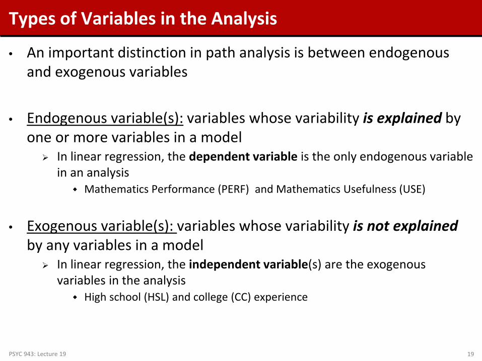
• An important distinction in path analysis is between endogenous and exogenous variables
• Endogenous variable(s): variables whose variability is explained by one or more variables in a model In linear regression, the dependent variable is the only endogenous variable
in an analysis Mathematics Performance (PERF) and Mathematics Usefulness (USE)
• Exogenous variable(s): variables whose variability is not explained by any variables in a model In linear regression, the independent variable(s) are the exogenous
variables in the analysis High school (HSL) and college (CC) experience
PSYC 943: Lecture 19 19
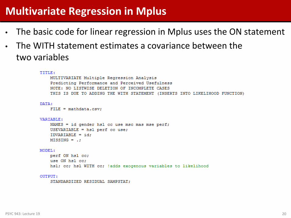
Multivariate Regression in Mplus
• The basic code for linear regression in Mplus uses the ON statement • The WITH statement estimates a covariance between the
two variables
PSYC 943: Lecture 19 20
Labeling Variables
• The endogenous (dependent) variables are: Performance (PERF) and Usefulness (USE)
• The exogenous (independent) variables are: High school (HSL) and college (CC) experience
PSYC 943: Lecture 19 21

Multivariate Regression Model Parameters • If we considered all four variables to be part of a multivariate normal
distribution, our unstructured (saturated) model would have a total of 14 parameters:
4 means 4 variances 6 covariances (4-choose-2 or 4*(4-1)/2))
• The model itself has 14 parameters:
4 intercepts 4 slopes 2 residual variances 1 residual covariance 2 exogenous variances 1 exogenous covariance
• Therefore, this model will fit perfectly – no model fit statistics will
be available Even without model fit, interpretation of parameters can proceed
PSYC 943: Lecture 19 22

Multivariate Linear Regression Path Diagram (Unstandardized Coefficients)
Mathematics Performance
(PERF)
High School Math Experience (HSL)
College Math Experience (CC)
6.623 (0.559)
.984 (0.120)
0.079 (0.027)
1.728 (0.138)
34.561 (2.758)
1.290 (0.456)
Direct Effect Residual (Endogenous) Variance
Exogenous Variances
Exogenous Covariances
Mathematics Usefulness
(USE)
243.303 (19.086)
2.901 (2.444)
1.466 (0.684)
0.206 (0.156)
Not Shown On Path Diagram: • 𝛽0𝑃𝑃𝑃𝑃 = 8.264 (0.629) • 𝛽0𝑈𝐻𝑃 = 43.129 (0.359) • 𝜇𝐻𝐻𝐻 = 4.922 (0.074) • 𝜇𝐶𝐶 = 10.330 (0.331)
Residual (Endogenous) Covariance
PSYC 943: Lecture 19 23
Interpreting Multivariate Regression Results for PERF
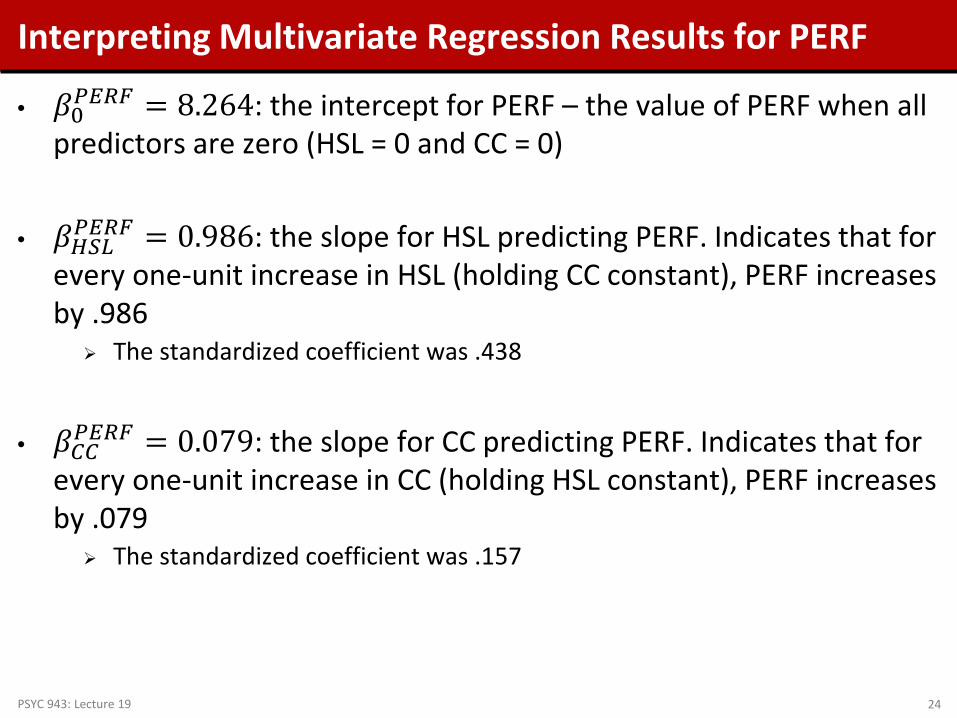
• 𝛽0𝑃𝑃𝑃𝑃 = 8.264: the intercept for PERF – the value of PERF when all predictors are zero (HSL = 0 and CC = 0)
• 𝛽𝐻𝐻𝐻𝑃𝑃𝑃𝑃 = 0.986: the slope for HSL predicting PERF. Indicates that for every one-unit increase in HSL (holding CC constant), PERF increases by .986 The standardized coefficient was .438
• 𝛽𝐶𝐶𝑃𝑃𝑃𝑃 = 0.079: the slope for CC predicting PERF. Indicates that for
every one-unit increase in CC (holding HSL constant), PERF increases by .079 The standardized coefficient was .157
PSYC 943: Lecture 19 24

Interpreting Multivariate Regression Results for USE
• 𝛽0𝑈𝐻𝑃 = 43.129: the intercept for USE – the value of USE when all predictors are zero (HSL = 0 and CC = 0)
• 𝛽𝐻𝐻𝐻𝑈𝐻𝑃 = 1.466: the slope for HSL predicting USE. Indicates that for every one-unit increase in HSL (holding CC constant), USE increases by 1.466 The standardized coefficient was .122
• 𝛽𝐶𝐶𝑈𝐻𝑃 = 0.206: the slope for CC predicting USE. Indicates that for every one-unit increase in CC (holding HSL constant), USE increases by .206. This was found to be not significant, meaning college experience did not predict perceived usefulness The standardized coefficient was .077
PSYC 943: Lecture 19 25

Interpretation of Residual Variances and Covariances
• 𝜎𝑒:𝑃𝑃𝑃𝑃2 = 6.623: the residual variance for PERF The R2 for PERF was .240 (the same as before)
• 𝜎𝑒:𝑈𝐻𝑃2 = 243.303: the residual variance for USE The R2 for USE was .024 (a very small effect)
• 𝜎𝑒:𝑃𝑃𝑃𝑃,𝑈𝐻𝑃 = 2.901: the residual covariance between USE and PERF This value was not significant, meaning we can potentially set its value to
zero and re-estimate the model
• Each of these variance describes the amount of variance not
accounted for in each dependent (endogenous) variable
PSYC 943: Lecture 19 26
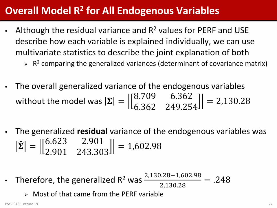
Overall Model R2 for All Endogenous Variables
• Although the residual variance and R2 values for PERF and USE describe how each variable is explained individually, we can use multivariate statistics to describe the joint explanation of both R2 comparing the generalized variances (determinant of covariance matrix)
• The overall generalized variance of the endogenous variables
without the model was 𝚺 = 8.709 6.3626.362 249.254 = 2,130.28
• The generalized residual variance of the endogenous variables was
𝚺� = 6.623 2.9012.901 243.303 = 1,602.98
• Therefore, the generalized R2 was 2,130.28−1,602.982,130.28
= .248 Most of that came from the PERF variable
PSYC 943: Lecture 19 27
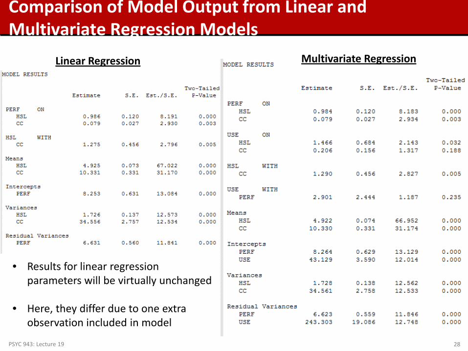
Comparison of Model Output from Linear and Multivariate Regression Models
Linear Regression Multivariate Regression
• Results for linear regression parameters will be virtually unchanged
• Here, they differ due to one extra observation included in model
PSYC 943: Lecture 19 28

Model Modification
• The residual covariance parameter (between PERF and USE) was not significant
• This means that after accounting for the relationship between HSL and CC with PERF along with HSL and CC with USE, the correlation between these two is zero Meaning we can likely remove the parameter from the model
• Removal of the parameter from the model would reduce the number of estimated parameters from 14 to 13 And would provide a mechanism to inspect goodness of fit of the
reduced model
PSYC 943: Lecture 19 29

Reduced Model Path Diagram
Mathematics Performance
(PERF)
High School Math Experience (HSL)
College Math Experience (CC)
𝜎𝑒:𝑃𝑃𝑃𝑃2
𝛽𝐻𝐻𝐻𝑃𝑃𝑃𝑃
𝛽𝐶𝐶𝑃𝑃𝑃𝑃
𝜎𝐻𝐻𝐻2
𝜎𝐶𝐶2
𝜎𝐻𝐻𝐻,𝐶𝐶
Direct Effect
Residual (Endogenous) Variance Exogenous Variances Exogenous Covariances
Mathematics Usefulness
(USE) 𝜎𝑒:𝑈𝐻𝑃2
𝛽𝐻𝐻𝐻𝑈𝐻𝑃
𝛽𝐶𝐶𝑈𝐻𝑃
PSYC 943: Lecture 19 30
Model Fit Information
• The Mplus Model Fit Information section provides model fit statistics that can help judge the fit of a model More frequently used in models with latent variables, but sometimes used
in path analysis
• The important thing to note is that not all “good-fitting” models are useful…
• The next few slides describe the statistics reported in this section of Mplus output
PSYC 943: Lecture 19 31

Log-likelihood Output
• The log-likelihood output section provides two log-likelihood values: H0: the log-likelihood from the model run in the analysis H1: the log-likelihood from the saturated (unstructured) model
• The saturated model (H1): All variances, covariances, and means estimated from Multivariate Normal Cannot do any better than the saturated model when using MVN If not all variables are normal, saturated model is harder to understand
• If these statistics are identical, then you are running a model equivalent to the saturated model No other model fit will be available or useful
PSYC 943: Lecture 19 32

Information Criteria Output
• The information criteria output provides relative fit statistics:
AIC: Akaike Information Criterion BIC: Bayesian Information Criterion (also called Schwarz’s criterion) Sample-size Adjusted BIC
• These statistics weight the information given by the parameter
values by the parsimony of the model (the number of model parameters) For all statistics, the smaller number is better
• The core of these statistics is -2*log-likelihood
PSYC 943: Lecture 19 33

Chi-Square Test of Model Fit
• The Chi-Square Test of Model Fit provides a likelihood ratio test comparing the current model to the saturated (unstructured) model: The value is -2 times the difference in log-likelihoods The degrees of freedom is the difference in the number of estimated
model parameters The p-value is from the Chi-square distribution
• If this test has a significant p-value:
The current model (H0) is rejected – the model fit is significantly worse than the full model
• If this test does not have a significant p-value:
The current model (H0) is not rejected – fits equivalently to full model
PSYC 943: Lecture 19 34

RMSEA (Root Mean Square Error of Approximation)
• The RMSEA is an index of model fit where 0 indicates perfect fit (smaller is better):
• RMSEA is based on the approximated covariance matrix
• The goal is a model with an RMSEA less than .05 Although there is some flexibility
• The result above indicates our model fits well (RMSEA of .035) Expected for 13 parameters (out of 14 possible)
PSYC 943: Lecture 19 35

CFI/TLI
• The CFI/TLI section provides two additional measures of model fit:
• CFI stands for Comparative Fit Index Higher is better (above .95 indicates good fit) Compares fit to independence model (uncorrelated variables)
• TLI stands for Tucker Lewis Index
Higher is better (above .95 indicates good fit)
• Both measures indicate good model fit (as they should for 13
parameters out of 14 possible)
PSYC 943: Lecture 19 36
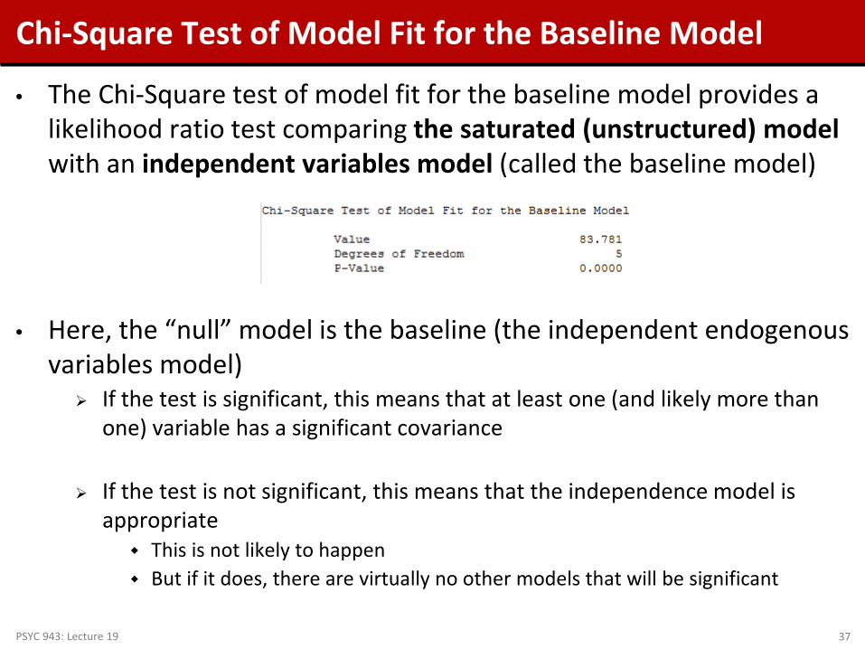
Chi-Square Test of Model Fit for the Baseline Model
• The Chi-Square test of model fit for the baseline model provides a likelihood ratio test comparing the saturated (unstructured) model with an independent variables model (called the baseline model)
• Here, the “null” model is the baseline (the independent endogenous variables model) If the test is significant, this means that at least one (and likely more than
one) variable has a significant covariance
If the test is not significant, this means that the independence model is appropriate This is not likely to happen But if it does, there are virtually no other models that will be significant
PSYC 943: Lecture 19 37
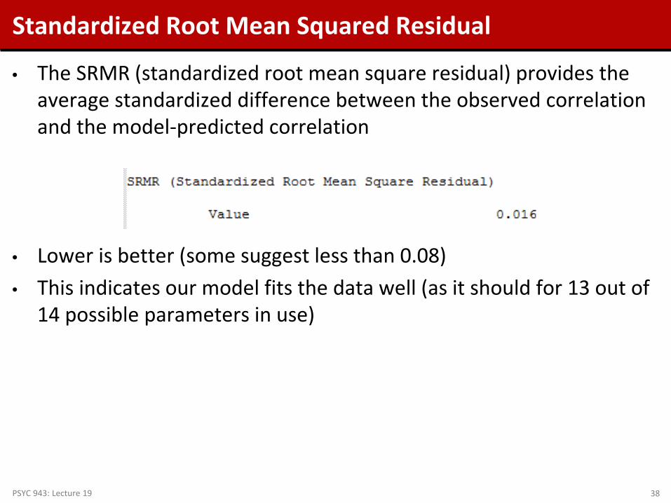
Standardized Root Mean Squared Residual
• The SRMR (standardized root mean square residual) provides the average standardized difference between the observed correlation and the model-predicted correlation
• Lower is better (some suggest less than 0.08) • This indicates our model fits the data well (as it should for 13 out of
14 possible parameters in use)
PSYC 943: Lecture 19 38

Comparing Our Full and Reduced Multivariate Regression Models
Full Model Reduced Model
PSYC 943: Lecture 19 39

Reduced Model Predicted and Residual Covariance Matrices – in Mplus • The REDUCED MODEL does not exactly reproduce the covariance
matrix of endogenous and exogenous variables:
• Note: the position of greatest discrepancy is for the covariance of PERF and USE The location where the residual covariance would matter
• The question of model fit statistics is whether “close fit” is close enough – does the model fit well enough
PSYC 943: Lecture 19 40

THE FINAL PATH MODEL: PUTTING IT ALL TOGETHER
PSYC 943: Lecture 19 41
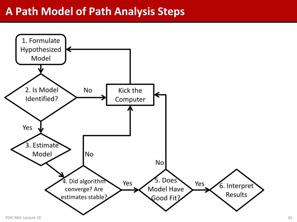
A Path Model of Path Analysis Steps
PSYC 943: Lecture 19 42
1. Formulate Hypothesized
Model
2. Is Model Identified?
Yes
No
3. Estimate Model
4. Did algorithm converge? Are
estimates stable?
No
Yes 5. Does Model Have
Good Fit?
No
Yes 6. Interpret Results
Kick the Computer
Identification of Path Models
• Model identification is necessary for statistical models to have meaningful results
From the error on the previous slide, we essentially had too many unknown values (parameters) and not enough places to put the parameters in the model
• For path models, identification can be a very difficult thing to understand We will stick to the basics here
• Because of their unique structure, path models must have identification in two ways:
“Globally” – so that the total number of parameters does not exceed the total number of means, variances, and covariances of the endogenous and exogenous variables
“Locally” – so that each individual equation is identified
• Identification is guaranteed if a model is both “globally” and
“locally” identified PSYC 943: Lecture 19 43

Global Identification: “T-rule”
• A necessary but not sufficient condition for a path models is that of having equal to or fewer model parameters than there are distributional parameters
• As the path models we discuss assume the multivariate normal
distribution, we have two matrices of parameters with which to work Distributional parameters: the elements of the mean vector and (or more
precisely) the covariance matrix
• For the MVN, the so-called T-rule states that a model must have equal to or fewer parameters than the unique elements of the covariance matrix of all endogenous and exogenous variables (the sum of all variables in the analysis) Let 𝑠 = 𝑝 + 𝑞, the total of all endogenous (p) and exogenous (q) variables Then the total unique elements are 𝑠(𝑠+1)
2
PSYC 943: Lecture 19 44

More on the “T-rule”
• The classical definition of the “T-rule” counts the following entities as model parameters:
Direct effects (regression slopes) Residual variances Residual covariances Exogenous variances Exogenous covariances
• Missing from this list are:
The set of exogenous variable means The set of intercepts for endogenous variables
• Each of the missing entities are part of the Mplus likelihood function, but
are considered “saturated” so no additional parameters can be added These do not enter into the equation for the covariance matrix of the
endogenous and exogenous variables
PSYC 943: Lecture 19 45

T-rule Identification Status
• Just-Identified: number of observed covariances = number of model parameters Necessary for identification, but no model fit indices available
• Over-Identified: number of observed covariances > number of model parameters Necessary for identification; model fit indices available
• Under-Identified: number of observed covariances < number of model parameters Model is NOT IDENTIFIED: No results available Do not pass go…do not collect $200
PSYC 943: Lecture 19 46
PSYC 943: Lecture 19 47
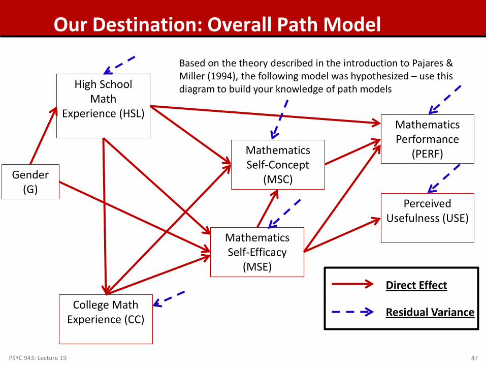
Our Destination: Overall Path Model
Mathematics Performance
(PERF) Mathematics Self-Concept
(MSC)
Perceived Usefulness (USE)
Mathematics Self-Efficacy
(MSE)
College Math Experience (CC)
High School Math
Experience (HSL)
Gender (G)
Direct Effect
Residual Variance
Based on the theory described in the introduction to Pajares & Miller (1994), the following model was hypothesized – use this diagram to build your knowledge of path models

Path Model Setup – Questions for the Analysis
• How many variables are in our model? 7 Gender, HSL, CC, MSC, MSE, PERF, and USE
• How many variables are endogenous? 6 HSL, CC, MSC, MSE, PERF, and USE
• How many variables are exogenous? 1 Gender
• Is the model recursive or non-recursive? Recursive – no feedback loops present
PSYC 943: Lecture 19 48

Path Model Setup – Questions for the Analysis
• Is the model identified? Check the t-rule first (and only as it is recursive) How many covariance terms are there in the all-variable matrix?
7∗ 7+1
2= 28
How many model parameters are to be estimated? 12 direct paths 6 residual variances 1 variance of the exogenous variable (19 model parameters for the covariance matrix) 6 endogenous variable intercepts
– Not relevant for t-rule identification, but counted in Mplus
• The model is over-identified 28 total variance/covariances but 19 model parameters We can use Mplus to run our analysis
PSYC 943: Lecture 19 49
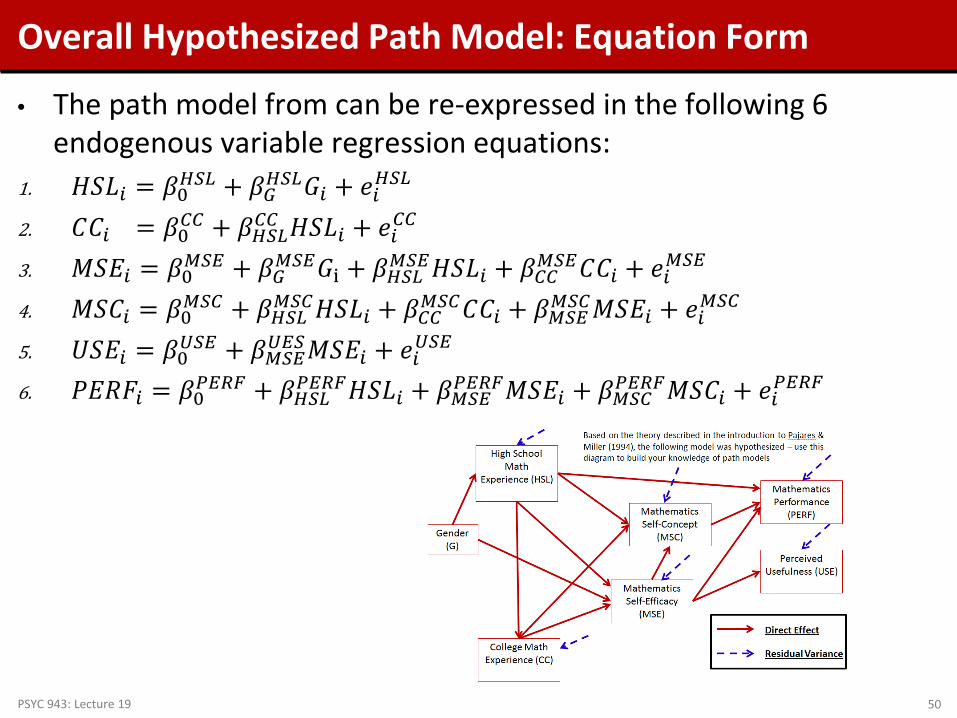
Overall Hypothesized Path Model: Equation Form
• The path model from can be re-expressed in the following 6 endogenous variable regression equations:
1. 𝐻𝐻𝐿𝑖 = 𝛽0𝐻𝐻𝐻 + 𝛽𝐺𝐻𝐻𝐻𝐺𝑖 + 𝑒𝑖𝐻𝐻𝐻 2. 𝐶𝐶𝑖 = 𝛽0𝐶𝐶 + 𝛽𝐻𝐻𝐻𝐶𝐶 𝐻𝐻𝐿𝑖 + 𝑒𝑖𝐶𝐶 3. 𝑀𝐻𝑃𝑖 = 𝛽0𝑀𝐻𝑃 + 𝛽𝐺𝑀𝐻𝑃𝐺i + 𝛽𝐻𝐻𝐻𝑀𝐻𝑃𝐻𝐻𝐿𝑖 + 𝛽𝐶𝐶𝑀𝐻𝑃𝐶𝐶𝑖 + 𝑒𝑖𝑀𝐻𝑃 4. 𝑀𝐻𝐶𝑖 = 𝛽0𝑀𝐻𝐶 + 𝛽𝐻𝐻𝐻𝑀𝐻𝐶𝐻𝐻𝐿𝑖 + 𝛽𝐶𝐶𝑀𝐻𝐶𝐶𝐶𝑖 + 𝛽𝑀𝐻𝑃𝑀𝐻𝐶𝑀𝐻𝑃𝑖 + 𝑒𝑖𝑀𝐻𝐶 5. 𝑈𝐻𝑃𝑖 = 𝛽0𝑈𝐻𝑃 + 𝛽𝑀𝐻𝑃𝑈𝑃𝐻𝑀𝐻𝑃𝑖 + 𝑒𝑖𝑈𝐻𝑃 6. 𝑃𝑃𝑃𝐹𝑖 = 𝛽0𝑃𝑃𝑃𝑃 + 𝛽𝐻𝐻𝐻𝑃𝑃𝑃𝑃𝐻𝐻𝐿𝑖 + 𝛽𝑀𝐻𝑃𝑃𝑃𝑃𝑃𝑀𝐻𝑃𝑖 + 𝛽𝑀𝐻𝐶𝑃𝑃𝑃𝑃𝑀𝐻𝐶𝑖 + 𝑒𝑖𝑃𝑃𝑃𝑃
PSYC 943: Lecture 19 50

Path Model Estimation in Mplus
• Having (1) constructed our model and (2) verified it was identified using the t-rule and that it is a recursive model, the next step is to (3) estimate the model with Mplus
• NOTE: Gender is not listed under the model statement It is a categorical variable (dummy coded 0/1)
• If added, Mplus treats it as continuous and plugs it into the MVN
log-likelihood This is a big no-no as it cannot be MVN
PSYC 943: Lecture 19 51
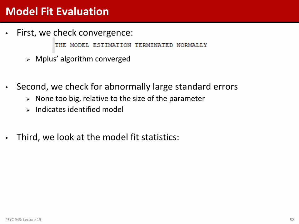
Model Fit Evaluation
• First, we check convergence: Mplus’ algorithm converged
• Second, we check for abnormally large standard errors
None too big, relative to the size of the parameter Indicates identified model
• Third, we look at the model fit statistics:
PSYC 943: Lecture 19 52

Model Fit Statistics
PSYC 943: Lecture 19 53
This is a likelihood ratio (deviance) test comparing our model (H0) with the saturated model – The saturated model fits much better (but that is typical).
The RMSEA estimate is 0.126. Good fit is considered 0.05 or less.
The CFI estimate is .917 and the TLI is .806. Good fit is considered 0.95 or higher.
This compares the independence model (H0) to the saturated model (H1) – it indicates that there is significant covariance between variables
The average standardized residual covariance is 0.056. Good fit is less than 0.05.
Based on the model fit statistics, we can conclude that our model does not do a good job of approximating the covariance matrix – so we cannot make inferences with these results (biased standard errors and effects may occur)
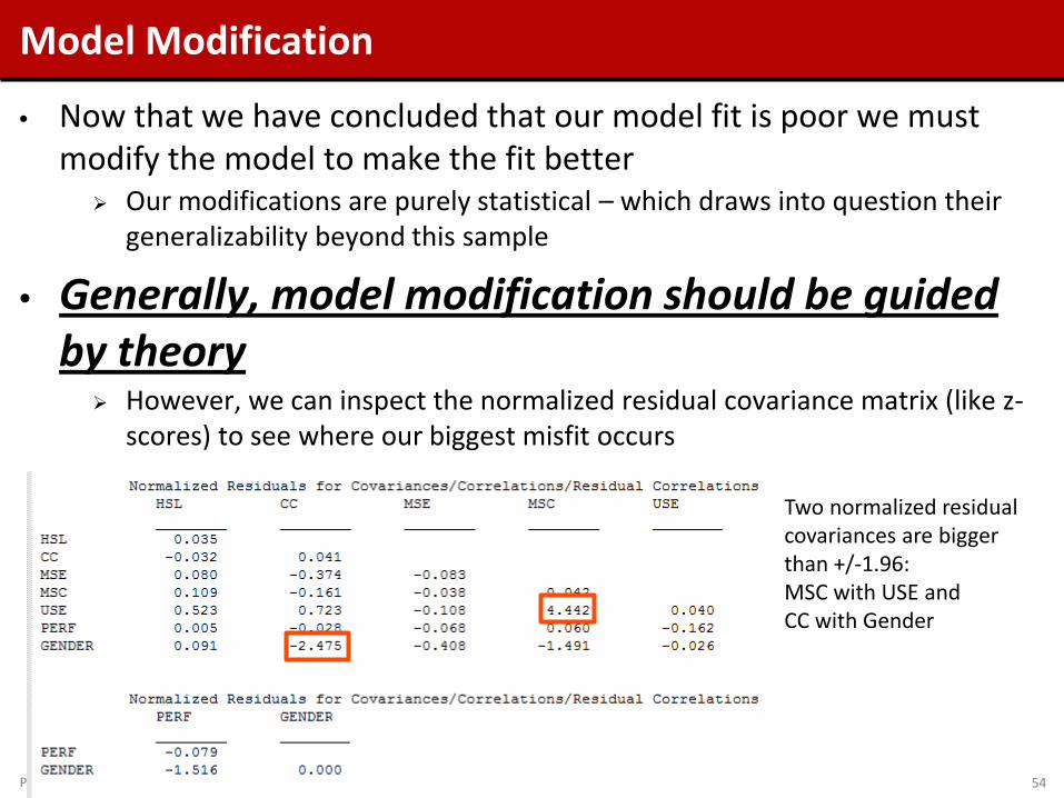
Model Modification
• Now that we have concluded that our model fit is poor we must modify the model to make the fit better Our modifications are purely statistical – which draws into question their
generalizability beyond this sample
• Generally, model modification should be guided by theory However, we can inspect the normalized residual covariance matrix (like z-
scores) to see where our biggest misfit occurs
PSYC 943: Lecture 19 54
Two normalized residual covariances are bigger than +/-1.96: MSC with USE and CC with Gender

PSYC 943: Lecture 19 55
Our Destination: Overall Path Model
Mathematics Performance
(PERF) Mathematics Self-Concept
(MSC)
Perceived Usefulness (USE)
Mathematics Self-Efficacy
(MSE)
College Math Experience (CC)
High School Math
Experience (HSL)
Gender (G)
The largest normalized covariances suggest relationships that may be present that are not being modeled:
For these we could: • Add a direct effect between G and CC • Add a direct effect between MSC and USE OR Add a residual
covariance between MSC and USE

Modification Indices: More Help for Fit
• As we used Maximum Likelihood to estimate our model, another useful feature is that of the modification indices Modification indices (also called Score or LaGrangian Multiplier tests) that
attempt to suggest the change in the log-likelihood for adding a given model parameter (larger values indicate a better fit for adding the parameter)
PSYC 943: Lecture 19 56
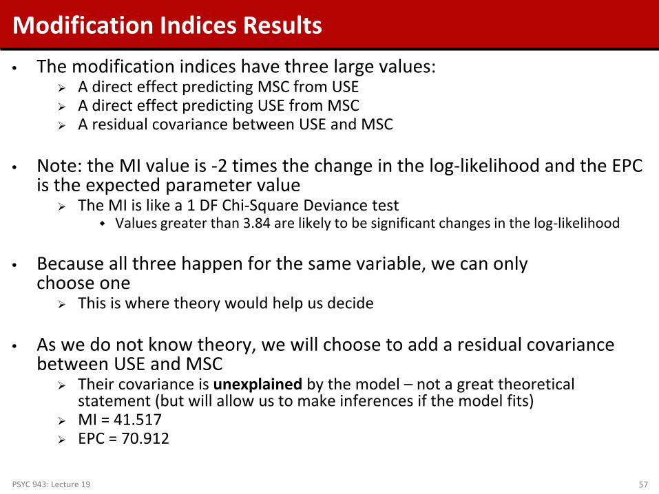
Modification Indices Results • The modification indices have three large values:
A direct effect predicting MSC from USE A direct effect predicting USE from MSC A residual covariance between USE and MSC
• Note: the MI value is -2 times the change in the log-likelihood and the EPC
is the expected parameter value The MI is like a 1 DF Chi-Square Deviance test
Values greater than 3.84 are likely to be significant changes in the log-likelihood
• Because all three happen for the same variable, we can only choose one
This is where theory would help us decide
• As we do not know theory, we will choose to add a residual covariance between USE and MSC
Their covariance is unexplained by the model – not a great theoretical statement (but will allow us to make inferences if the model fits)
MI = 41.517 EPC = 70.912
PSYC 943: Lecture 19 57
PSYC 943: Lecture 19 58
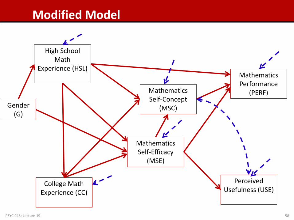
Modified Model
Mathematics Performance
(PERF) Mathematics Self-Concept
(MSC)
Perceived Usefulness (USE)
Mathematics Self-Efficacy
(MSE)
College Math Experience (CC)
High School Math
Experience (HSL)
Gender (G)

Assessing Model fit of the Modified Model
• Now we must start over with our path model decision tree The model is identified (now 20 parameters < 28 covariances) Mplus estimation converged; Standard errors look acceptable
• Model fit statistics:
PSYC 943: Lecture 19 59
The comparison with the saturated model suggests our model fits statistically
The RMSEA is 0.049, which indicates good fit
The CFI and TLI both indicate good fit
The SRMR also indicates good fit
Therefore, we can conclude the model adequately approximates the covariance matrix – meaning we can now inspect our model parameters…but first, let’s check our residual covariances and modification indices
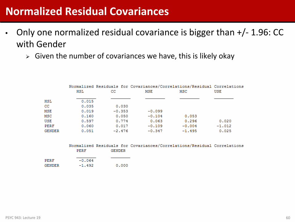
Normalized Residual Covariances
• Only one normalized residual covariance is bigger than +/- 1.96: CC with Gender Given the number of covariances we have, this is likely okay
PSYC 943: Lecture 19 60

Modification Indices
• Now, no modification indices are glaringly large, although some are bigger than 3.84 We discard these as our model now fits (and adding them may not be
meaningful)
PSYC 943: Lecture 19 61
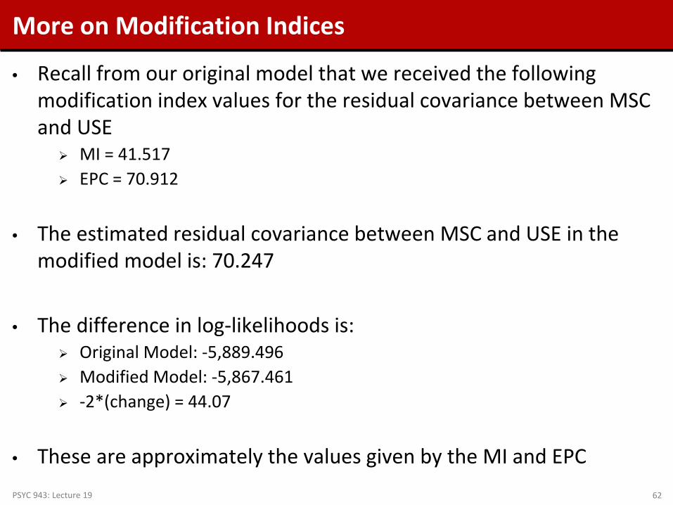
More on Modification Indices
• Recall from our original model that we received the following modification index values for the residual covariance between MSC and USE MI = 41.517 EPC = 70.912
• The estimated residual covariance between MSC and USE in the modified model is: 70.247
• The difference in log-likelihoods is: Original Model: -5,889.496 Modified Model: -5,867.461 -2*(change) = 44.07
• These are approximately the values given by the MI and EPC PSYC 943: Lecture 19 62

Model Parameter Investigation
PSYC 943: Lecture 19 63
There are two direct effects that are non-significant:
𝛽𝐺𝐻𝐻𝐻 = 0.208 𝛽𝐻𝐻𝐻𝑃𝑃𝑃𝑃 = 0.153
We can leave these in the model, but the overall path model seems to suggest they are not needed So, I will remove them and re-estimate the model

PSYC 943: Lecture 19 64
Modified Model #2
Mathematics Performance
(PERF) Mathematics Self-Concept
(MSC)
Perceived Usefulness (USE)
Mathematics Self-Efficacy
(MSE)
College Math Experience (CC)
High School Math
Experience (HSL)
Gender (G)

Model #2: Model Fit Results
• We have: an identified model, a converged algorithm, and stable standard errors, so model fit should be inspected Next – inspect model fit Model fit seems to not be as good as we would think
• Again, the largest normalized residual covariance is that of GENDER
and CC MI for direct effect of GENDER on CC is 6.595, indicating that adding this
parameter may improve model fit
• So, we will now add a direct effect of Gender on CC
PSYC 943: Lecture 19 65
PSYC 943: Lecture 19 66
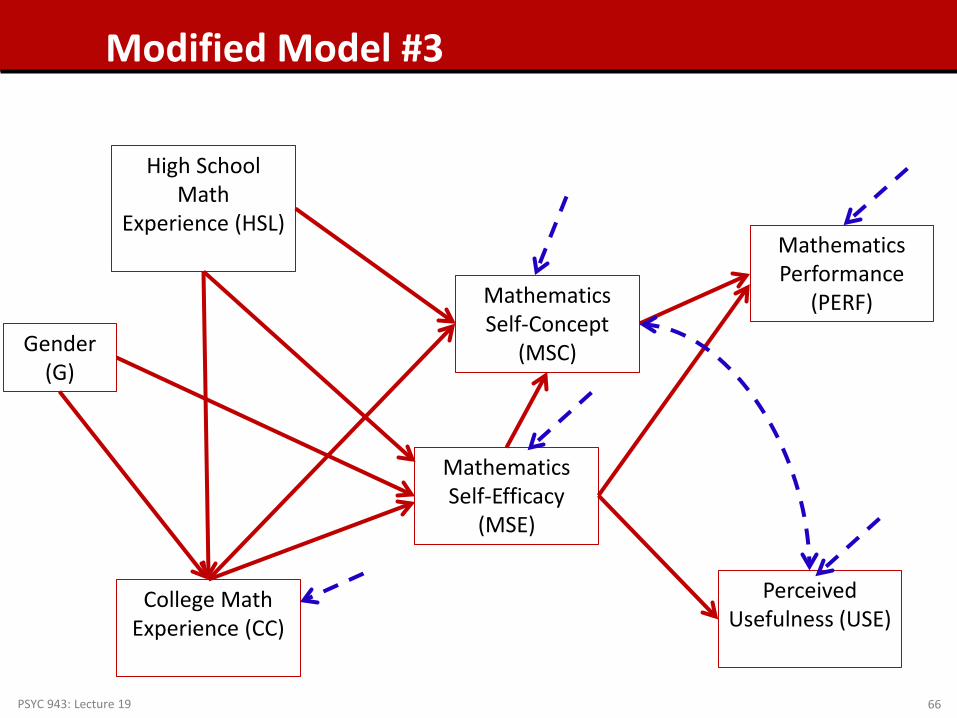
Modified Model #3
Mathematics Performance
(PERF) Mathematics Self-Concept
(MSC)
Perceived Usefulness (USE)
Mathematics Self-Efficacy
(MSE)
College Math Experience (CC)
High School Math
Experience (HSL)
Gender (G)

Model #3: Model Fit Results
• We have: an identified model, a converged algorithm, and stable standard errors, so model fit should be inspected Next – inspect model fit Model fit seems to be very good
• No normalized residual covariances are larger than +/- 1.96 – so we appear to have good fit
• No Modification Indices are larger than 3.84 We will leave this model as-is and interpret the results
PSYC 943: Lecture 19 67

Model #3 Parameter Interpretation
Interpret each of these parameters as you would in regression: A one-unit increase in HSL brings about a .707 unit increase in CC, holding gender constant
PSYC 943: Lecture 19 68
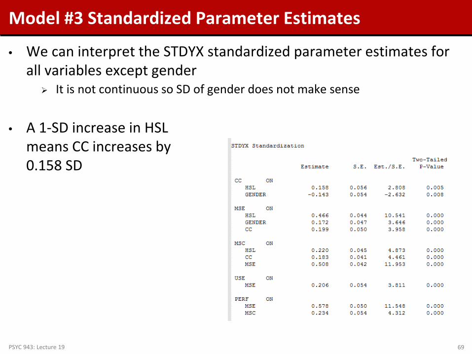
Model #3 Standardized Parameter Estimates
• We can interpret the STDYX standardized parameter estimates for all variables except gender It is not continuous so SD of gender does not make sense
• A 1-SD increase in HSL means CC increases by 0.158 SD
PSYC 943: Lecture 19 69

Model #3 STDY Interpretation
• The STDY standardization does not standardize by the SD of the X variable So it’s interpretation makes sense for Gender (1 = male)
Here, males have an average CC (intercept) that is -.301 SD lower than females
PSYC 943: Lecture 19 70

Overall Model Interpretation
• High School Experience and Gender are significant predictors of College Experience Men lower than women in College Experience More High School Experience means more College Experience
• High School Experience, College Experience, and Gender are significant predictors of Math Self-Efficacy More High School and College Experience means higher Math Self-Efficacy Men have higher Math Self-Efficacy than Women
PSYC 943: Lecture 19 71

Overall Model Interpretation, Continued
• High School Experience, College Experience, and Math Self-Efficacy are significant predictors of Math Self-Concept More High School and College Experience and higher Math Self-Efficacy
mean higher Math Self-Concept
• Higher Math Self-Efficacy means significantly higher
Perceived Usefulness
• Higher Math Self-Efficacy and Math Self-Concept result in higher Math Performance scores
• Math Self-Concept and Perceived Usefulness have a significant residual covariance
PSYC 943: Lecture 19 72

Model Interpretation: Explained Variability
• The R2 for each endogenous variable: CC – 0.046 MSE – 0.306 MSC – 0.509 USE – 0.042 PERF – 0.568
• Note how college experience and perceived usefulness both have low percentages of variance accounted for by the model We could have increased the R2 for USE by adding the direct path between
MSC and USE instead of the residual covariance
PSYC 943: Lecture 19 73
ADDITIONAL MODELING CONSIDERATIONS IN PATH ANALYSIS
PSYC 943: Lecture 19 74
Additional Modeling Considerations
• The path analysis we just ran was meant to be an introduction to the topic and the field It is much more complex than what was described
• In particular, our path analysis assumed all variables to be
Continuous and Multivariate Normal Measured with perfect reliability
• In reality, neither of these are true
• Structural equation models (path models with latent variables) will
help with variables with measurement error See PSYC 948 in the Spring
• Modifications to model likelihoods or different distributional
assumptions will help with the normality assumption See next lecture
PSYC 943: Lecture 19 75
About Causality
• You will read a lot of talk about path models indicating causality, or how path models are causal models
• It is important to note that causality can rarely, if ever, be inferred on the basis of observational data Experimental designs with random assignment and manipulations of factors
will help detect causality
• With observational data, about the best you can say is that IF your model fits, then causality is ONE reason But realistically, you are simply describing covariances of variables in more
fancy ways/parameters
• If your model does not fit, the causality is LIKELY not occurring But still could be possible if important variables are omitted
PSYC 943: Lecture 19 76

CONCLUDING REMARKS
PSYC 943: Lecture 19 77

Path Analysis: An Introduction
• In this lecture we discussed the basics of path analysis Model specification/identification Model estimation Model fit (necessary, but not sufficient) Model modification and re-estimation Final model parameter interpretation
• There is a lot to the analysis – but what is important to remember is the over-arching principal of multivariate analyses: covariance between variables is important Path models imply very specific covariance structures The validity of the results hinge upon accurately finding an approximation to
the covariance matrix
PSYC 943: Lecture 19 78