an open-source python-based boundary-element method code

Modeling, Identification and Control, Vol. 42, No. 2, 2021, pp. 47–81, ISSN 1890–1328

An Open-Source Python-Based Boundary-ElementMethod Code for the Three-Dimensional,Zero-Froude, Infinite-Depth, Water-Wave

Diffraction-Radiation Problem

S. Viswanathan 1 C. Holden 1 O. Egeland 1 M. Greco 2

1Department of Mechanical and Industrial Engineering, Norwegian University of Science and Technology (NTNU),N0-7041 Trondheim, Norway. E-mail: {savin.viswanathan,christian.holden,olav.egeland}@ntnu.no

2Department of Marine Technology, Norwegian University of Science and Technology (NTNU), N0-7491 Trond-heim, Norway; Institute of Marine Engineering, CNR-INM, Italy. E-mail: [email protected]

Abstract

In this paper, a new open-source implementation of the lower-order, 3-D Boundary Element Method(BEM) of solution to the deep-water, zero Froude-number wave-body interaction problem is described. Avalidation case for OMHyD, the new open-source package, is included, where the outputs are compared toresults obtained using the widely used frequency-domain hydrodynamic analysis package ANSYS-AQWA.The theory behind the solution to the diffraction-radiation problem is re-visited using the Green functionmethod. The Hess and Smith panel method is then extended to the case of a floating object using theimage-source to impose the wall condition at the free-surface, and a wavy Green function component toaccount for presence of free-surface waves. An algorithm for computer implementation of the procedure isdeveloped and subsequently implemented in PYTHON. The wavy part of the Green function is determinedusing a verified and published FORTRAN code by Teleste and Noblesse, wrapped for PYTHON using theFortran to Python (F2PY) interface. Results are presented for the various stages of implementationviz. panelling, body in infinite fluid domain, effect of the free-surface, and effect of surface-waves. Thehydrodynamic coefficients obtained from this preliminary frequency-domain analysis are shown to be insatisfactory agreement with ANSYS-AQWA results. Conclusions are drawn based on the performance ofthe code, followed by suggestions for further improvement by including the removal of irregular-frequencies,multi-body interactions, and bottom interference, which are not considered in the present implementation.

Keywords: Wave-body interaction, 3D boundary-element method, frequency-domain hydrodynamic anal-ysis, diffraction-radiation loads

1. Introduction

In offshore applications, there is often a need to simu-late the dynamic response of ships and floaters to theenvironmental loads due to the wind, waves, and cur-rents, and to the operational loads from cranes, stationkeeping systems, risers, pipe-lay systems etc.

The problem of a ship in waves is commonly referredto as the sea-keeping problem (Fossen, 2011, pp. 11–12), and involves frequency dependent hydrodynamicparameters. Determination of these parameters re-quires numerical solutions to the wave-body interactionproblem. The theory for this is well developed and

doi:10.4173/mic.2021.2.2 c© 2021 Norwegian Society of Automatic Control

http://dx.doi.org/10.4173/mic.2021.2.2

Modeling, Identification and Control

is implemented in commercial frequency-domain hy-drodynamic analysis packages like WAMIT, ANSYS-AQWA etc.

The multiphysical simulation of marine operationscan be done in a component-oriented modeling ap-proach where models representing each component ofthe system are interconnected, as demonstrated in(Viswanathan and Holden, 2019). The interconnectionof the models can be done in a co-simulation arrange-ment, or as one integrated model. The interconnectionscan be implemented using either commercial MODEL-ICA environments, or the open-source OpenModelicaenvironment.

Commonly used hydrodynamic analysis packageslike WAMIT and ANSYS-AQWA do not render them-selves to the open-source philosophy of OpenModelica.This makes the use of component models requiring in-puts from such software cumbersome. This is espe-cially true if there is a need to recalculate the hydro-dynamic parameters, e.g. due to a large change in themean position of the wetted surface, based on whichthe hydrodynamic parameters are calculated. A fewopen-source, frequency domain, hydrodynamic analy-sis packages like NeMOH exist, but with limitations inthe number of nodes, documentation, and simulationtimes as discussed in (Penalba et al., 2017).

On this note, we decided to develop an open-source software package for frequency domain hydro-dynamic analysis, which makes it possible to calculatethe required hydrodynamic parameters for use in acomponent-oriented modeling-and-simulation packagebased on OpenModelica. The new hydrodynamic anal-ysis package, OMHyD, is a three-dimensional, lower-order boundary-element method program, utilizing thesource formulation, and the zero-speed, infinite-depth,free-surface Green function. This paper presents thetheory and implementation details behind the develop-ment of OMHyD. The program package is implementedin PYTHON, and the developed code is made publicat github.com/Savin-Viswanathan/OMHyD-PA.

The paper includes a validation of the program pack-age for a cuboidal body where the parameters fromOMHyD are compared to the parameters generated forthe same body in ANSYS-AQWA.

Lagrange introduced the concept of the velocity po-tential in the 1780’s. Lamb (1879, Ch. 3) appliedGreen’s second identity to express the velocity po-tential, in the case of a body in an infinite fluid do-main, as the effect of a distribution of simple and dou-ble sources over the body boundary. John (1949) ob-tained expressions for the wave function in the caseof regular incident waves interacting with bodies satis-fying certain geometric assumptions. Hess and Smith(1967) pioneered a method to calculate the flow around

arbitrary, non-lifting, 3D bodies, in an infinite fluiddomain, based on simple source distributions on flatquadrilateral panels approximating the body surface,also referred to as the panel-method. Hess and Wilcox(1969) reported the progresses in the extension of thepanel-method in evaluating the velocity potential by asmall oscillating body in the presence of a free surface.Wehausen (1971) formulated a potential flow methodfor wave-induced motions of free-floating bodies, anddemonstrated the agreement of numerical calculationsbased on the diffraction-radiation formulation with ex-perimental results. Newman and Sclavounos (1988)presented the WAMIT software package, which wasbased on the panel method, for analysis of water-waveradiation and diffraction.

Further, (Newman, 1977, Ch. 6) and (Faltinsen,1990, Ch. 3) discussed the wave-body interactionproblem within the confines of potential theory. TheGreen’s theorem and the distribution of singularitiesis discussed in (Newman, 1977, Ch. 4). Garrison(1978) described the use of the Green function to rep-resent the source potential in calculating wave-loads onlarge floating-bodies. Numerical implementation of thepanel-method was described in (Faltinsen, 1990, Ch.4). Telste and Noblesse (1986) presented a method fornumerically evaluating the free surface Green functionand its gradient, in deep-water, and zero forward-speedconditions, and also made available the print-out of theassociated FORTRAN subroutine in their appendix.

McTaggart (2002) described a method for comput-ing three-dimensional hydrodynamic coefficients in thefrequency domain, using the Green function given in(Telste and Noblesse, 1986). Guha (2012) describedthe development of a three-dimensional panel-methodusing the Green function, as described by Telste andNoblesse (1986), and based on the overall approachby McTaggart (2002). The software implementationsof McTaggart (2002) and Guha (2012) have not beenmade publicly available.

In implementing the PYTHON code for OMHyD, wefollow the general framework presented in (McTaggart,2002) and (Guha, 2012).

The paper proceeds with a brief description of thetheory behind the wave-body interaction problem, andthe Green function method. A discussion on the ex-tension of the Hess and Smith panel method to thecase of an object in the presence of free-surface wavesis then presented, along with analytical expressions forthe source potential, and its derivatives. The method ofdetermination of the wavy part of the Green function,and its derivatives is also discussed. Subsequently, thealgorithm for OMHyD is described, and results of theimplementation discussed thereafter.

48

https://github.com/Savin-Viswanathan/OMHyD-PA

Viswanathan et.al., “Pythonic approach to BEM”

2. Theory

In the discussions that follow, ~x represents a vector,and x represents a unit vector. u represents the timederivative of u.

2.1. The Wave-Body Interaction Problem

Considering the physical effects of a floating object in-teracting with incident waves, we observe the following(Wehausen, 1971):

1. The fluid pressure force on the body changes as aresult of the incident waves, and this causes thebody to oscillate about its mean position.

2. The presence of the body scatters the incidentwave in all directions, and these scattered wavesexert associated fluid pressure forces on the body,affecting its motion.

3. The motion of the body generates radiation wavesmoving out in all directions, and these waves in-turn exert associated fluid pressure forces on thebody.

Within assumptions of potential flow and linearizedboundary conditions, considering the steady-state in-teraction of a floating object with a regular-wave prop-agating in deep water, on an infinite free-surface, thetotal velocity potential in the vicinity of the float-ing object in regular waves can be expressed as (Mc-Taggart, 2002), (Wehausen, 1971) and (Faltinsen andMichelsen, 1975):

Φ(~x, γ, t) =

ϕ0(~x, γ) + ϕ7(~x, γ) +

6∑j=1

ηjϕj(~x)

eiωt.(1)

Here, ϕ0 is the spatial component of incident wavepotential, ϕ7 is the scattered wave potential, ϕj=1,...,6

represent the radiation potential for unit amplitude os-cillation in the jth DoF (mode) of the body, and ηj isthe amplitude of oscillation for mode j. i is the imagi-nary unit. ~x is the position vector xı+ y+ zk of anyfield point, and γ is the angle of incidence of the wavewith respect to the positive direction of the x axis ofa right-handed coordinate system with its origin lyingon the water plane directly above the centre of gravityof the floating object. The notation is illustrated inFigure 1.

For deep-water, the spatial component of the inci-dent wave potential is expressed as

ϕ0(~x, γ, ω, ζa) = igζaωekze−ik(x cos γ−y sin γ). (2)

η6 η4

η1η3

η2 η5

X

Z

Y

wave crests

direction ofwave propagation

γ

∞

∞

∞

Figure 1: Definition sketch

Here, ζa [m] is the wave amplitude, and k [m−1] is thewave number, which is related to the wave frequencyω [rad/s] through the dispersion relation

ω2 = gk tanh kh, (3)

where, g [m/s2] is the acceleration due to gravity, andh [m] is the water depth.

Further, ϕj , j ∈ {1, . . . , 7} must satisfy:

∂2ϕj∂x2

+∂2ϕj∂y2

+∂2ϕj∂z2

= 0, in the fluid domain (4)

−ω2ϕj + g∂ϕj∂z

= 0, on z = 0 (5)

∂ϕj∂z

= 0, on z = −∞. (6)

In addition, ϕjηj , j ∈ {1, . . . , 6} and ϕ7 must satisfythe linearized kinematic body-boundary condition

∂ϕj∂n

=

{iωnj , j = 1, . . . 6

−∂ϕ0

∂n , j = 7

∣∣∣∣∣S0

. (7)

Here, ∂∂n is the normal derivative in the direction of

the unit outward normal n to the submerged surface ofthe body in its mean position, S0. The scalars nj arethe components of the generalized normal vectors

n = (n1, n2, n3), (8)

~x× n = (n4, n5, n6). (9)

For further details see (Wehausen, 1971), (Faltinsenand Michelsen, 1975), and (Milgram, 2003, pp. 238,241, and 266 ).

It is noted that waves originating as a consequenceof incident waves being scattered by the body surface,

49


and those originating due to the motions of the body,must be outgoing, and should have proper amplitudebehavior at infinity. This imposes an additional radi-ation condition on ϕj , j ∈ {1, . . . , 7}. Details can befound in (Wehausen, 1971) and (John, 1949).

In determining ϕj=1,...,7, we make use of the Greenfunction method as described in Sec. 2.2.

2.1.1. The Bernoulli equation

The Bernoulli equation relates the fluid pressure andthe velocity potential in the fluid domain.

From the linearized form of the Bernoulli equation,(Faltinsen, 1990, (2.4)), we get

p(~x, t) = −ρ∂Φ(~x, t)

∂t︸︷︷︸Hydrodynamic pressure

−ρgz︸︷︷︸Hydrostatic pressure

. (10)

With reference to (1), the total velocity potential Φis expressed as the sum of the diffraction potential ΦD,and the radiation potential ΦR. Thus,

Φ = ΦD + ΦR, (11)

where,

ΦD = [ϕ0(~x, γ) + ϕ7(~x, γ)] eiωt (12)

ΦR =

6∑j=1

ηjϕj(~x)eiωt. (13)

Consider the wetted body surface S(~ξ), ~ξ = (ξ, η, ζ).Here the ξηζ frame is the body coordinate frame, whichcoincides with the global xyz coordinate frame. At themean position, let the wetted body surface be denotedby S0(~ξ). To determine the linear terms of the pressureloads, the hydrostatic pressure should be integratedover the instantaneous position of the body, while thehydrodynamic pressure should be integrated along themean wetted surface. Thus, from (10)

O(1)

{∫∫S

p(~ξ, t)nk(~ξ)dS

}= −ρ

∫∫S0

∂[ΦD(~ξ, t) + ΦR(~ξ, t)]

∂tnk(~ξ)dS︸︷︷︸

Hydrodynamic pressure Load

−ρg∫∫

S

ζnk(~ξ)dS︸︷︷︸Hydrostatic pressure load

, k = 1, . . . , 6. (14)

Here nk is defined in (8) and (9).The hydrostatic pressure loads give the mean buoy-

ancy. The component of the hydrodynamic pressureload due to the diffraction potential gives the wave-excitation loads and that due to the radiation potentialgives the wave-radiation loads on the oscillatory body.

2.1.2. The diffraction problem: The Froude–Kryloffand diffraction loads

With reference to (12), the diffraction potential at thebody surface is written as

ΦD(~ξ, t) = Φ0(~ξ, t) + Φ7(~ξ, t). (15)

With reference to the first term on the R.H.S. of (14),the wave-excitation load along the kth DoF is given by

F ek (t) =−ρ∫∫

S0

∂Φ0(~ξ, t)


Froude–Kryloff loads

− ρ∫∫

S0

∂Φ7(~ξ, t)


Diffraction loads

,

k = 1, . . . , 6. (16)

Here, the loads due to the incident wave potential Φ0

are commonly referred to as the Froude–Kryloff loads,and those associated with the scattered wave potentialΦ7, are referred to as the diffraction loads (Faltinsen,1990, (3.36)).

2.1.3. The radiation problem: Added-mass anddamping

With reference to (13), the radiation potential at thebody surface is written as

ΦR(~ξ, t) =

6∑j=1

ϕj(~ξ){ηjeiωt}, (17)

where ηj is the amplitude of motion in mode j, and ϕjis the spatial component of the complex potential dueto unit amplitude of motion in the jth DoF.

With reference to the first term on the R.H.S. of (14),the wave-radiation load along the kth DoF is given by

F rk (t) = −ρ∫∫

S0

∂ΦR(~ξ, t)

∂tnk(~ξ)dS. (18)

The wave-radiation load along the kth DoF due to bodyoscillation along the jth DoF is now expressed as

F rk,j(t) = −ρ∫∫

S0

{ ˙ηjeiωt}[R{ϕj(~ξ)}

+ iI{ϕj(~ξ)}]nk(~ξ)dS

=

[− ρω

∫∫S0

I{ϕj(~ξ)}nk(~ξ)dS

]︸︷︷︸

added mass

¨ηjeiωt

+

[−ρ∫∫

S0

R{ϕj(~ξ)}nk(~ξ)dS

]︸︷︷︸

damping

˙ηjeiωt.

(19)

50


Here, R and I represent the real and imaginary com-ponents, respectively, and the dot and double-dot rep-resent time derivatives.

The load component proportional to the accelerationis referred to as the added mass, and that proportionalto the velocity is referred to as damping. Thus,

Akj = − ρω

∫∫S0

I{ϕj(~ξ)}nk(~ξ)dS (20)

Bkj = −ρ∫∫

S0

R{ϕj(~ξ)}nk(~ξ)dS, (21)

where Akj is referred to as the added-mass, and Bkj isreferred to as the radiation-damping, in the kth direc-tion due to wave radiation in the jth mode of oscilla-tion. For details, see (Faltinsen and Michelsen, 1975),and (Guha et al., 2016).

2.2. The Green Function Method

2.2.1. The free-space Green function

Consider a body placed inside an unbounded fluid do-main. The velocity potential at any field point Q inthe fluid domain is given by (Lamb, 1879, p. 60)

ϕQ =−1

4π

∫∫S

(∂ϕ

∂n− ∂ϕ′

∂n

)1

rdS (22)

i.e., as the resultant potential due to the distribution

of simple sources of strength(∂ϕ∂n −

∂ϕ′

∂n

)on the body

surface, and where ϕ and ϕ′ correspond to potentialsoutside and inside the closed body surface S, respec-tively. Here, r is the distance between the field pointQ(~x), and the source located at P (~ξ), on the body sur-face, where ~x = (x, y, z) is the position vector of the

field point, and ~ξ = (ξ, η, ζ) is the position vector ofthe source point on the body surface.

The next step is to define the free-space Green func-tion G∗(~x, ~ξ) = −1

4πr , which is analogous to the source-

potential, and the source density σ(~ξ) =(∂ϕ∂n −

∂ϕ′

∂n

).

We may then express the potential at any field pointas

ϕ(~x) =

∫∫S

σ(~ξ)G∗(~x; ~ξ)dS (23)

2.2.2. The free-surface Green function

In cases where the body may move in a fluid do-main bounded by other boundaries such as the free-surface, the fluid bottom, or lateral boundaries, addi-tional boundary conditions are imposed on the prob-lem.

The Green function should satisfy the Laplace equa-tion in the fluid domain, and all boundary conditionssatisfied by ϕ, except the body boundary condition.

Determination of such a Green function provides anexplicit solution to the potential. However, this typeof source potential is not known except for some verysimple body geometries (Newman, 1977, pp. 138–137).

(Wehausen and Laitone, 1960) gives expressions forthe finite-depth Green function. Kim (2008) gives adetailed derivation for the deep-water Green function.

(Telste and Noblesse, 1986) gives expressions forthe infinite-depth free-surface Green function and itsderivatives, with the velocity potential expressed asR{G(~x, ~ξ; f)e−iωt}. These expressions, modified for atemporal component of eiωt of the velocity potential,are given as

G(~x, ~ξ; f) =−1

4π

(1

r+

1

r′

)+ G(~x, ~ξ, f) (24)

where,

G(~x, ~ξ, f) =−1

4π[2f {R0(h, v)− iπJ0(h) exp(v)}]

(25)

f =ω2L

g, L being the reference length (26)

ρ ={

(x− ξ)2 + (y − η)2}

(27)

r ={ρ2 + (z − ζ)2

}1/2(28)

r′ ={ρ2 + (z + ζ)2

}1/2(29)

h = fρ (30)

v = f(z + ζ) (31)

(ξ,η,ζ≤0)

(ξ,η,-ζ≥0)

(x,y,z≤0)

Singular point

Image singular point

Field point

r'=d/f

r

(x-ξ)2+(y-η)2= h/f

z+ζ=v/f

Figure 2: Definition sketch [adapted from (Telste andNoblesse, 1986)]

Considering the R.H.S. of (24), and the definitionsketch in Figure 2, we make the interpretations that

51


the first term represents the sum of the source poten-tial at a field point ~x = (x, y, z) due to a unit source

at ~ξ = (ξ, η, ζ), and the image-source, having coordi-nates (ξ, η,−ζ). This image source (Newman, 1977, p.160) accounts for the interaction between the body andthe linearized free surface which behaves like a rigidboundary. The second term G(~x, ~ξ, f) is the oscillat-ing potential at the field point due to the oscillation ofthe source strength, to account for the oscillating flowdue to the presence of waves, and therefore referred toas the wavy part of the Green function.

The wavy part of the Green function given by (25)has partial derivatives:

∂G

∂x=∂G

∂ρ

(x− ξ)ρ

(32)

∂G

∂y=∂G

∂ρ

(y − η)

ρ(33)

∂G

∂z=

1

4π

[− 2f2

{1

d+R0(h, v)

− iπJ0(h)ev}]

(34)

where,

∂G

∂ρ=

1

4π

[2f2 {R1(h, v) + iJ1(h)ev}

](35)

d = (h2 + v2)1/2 = fr′. (36)

Here, J0(h) and J1(h) are usual Bessel functions ofthe first kind, and R0(h, v) and R1(h, v) are real func-tions, which are evaluated by the FORTRAN subrou-tine GRADIF, the printout of which, is available in theappendix of (Telste and Noblesse, 1986).

Numerous works cite this method and it has beenvalidated in (Chakrabarti, 2001).

2.2.3. Determination of the source densitydistribution

Once the Green function is determined, the solutionfor ϕj , j ∈ {1, . . . , 7} can be expressed as given in(Faltinsen and Michelsen, 1975) by

ϕj(~x) =

∫∫S0

σj(~ξ)G(~x, ~ξ; f)dS, (37)

where G is the deep-water Green Function given by(24).

The application of the body boundary conditiongiven by (7) to the above gives

∂

∂n(~x)

∫∫S0

σj(~ξ)G(~x, ~ξ; f)dS

=

{iωnj(~x), j = 1, . . . 6

− ∂ϕ0

∂n(~x) , j = 7

∣∣∣∣∣~x∈S0

. (38)

Here, the integral over the body surface is to be in-terpreted in the Cauchy principal value sense, sinceit is singular when ~x = ~ξ. The limiting process ofthe Cauchy principal-value gives (Malenica and Chen,1998):

∂

∂n(~x)

∫∫S0

σj(~ξ)G(~x, ~ξ; f)dS

=σj(~x)

2+

∫∫S0

σj(~ξ)∂G(~x, ~ξ; f)

∂n(~x)dS (39)

Thus, (38) gives

σj(~x)

2+

∫∫S0

σj(~ξ)∂G(~x, ~ξ; f)

∂n(~x)dS

=

{iωnj(~x), j = 1, . . . 6

− ∂ϕ0

∂n(~x) , j = 7

∣∣∣∣∣~x∈S0

. (40)

From this the source density distributions associatedwith the diffraction and radiation problems can be de-termined, provided we have knowledge about the in-cident potential, the generalized normals to the bodysurface, and the normal derivative of the associatedGreen function.

The numerical procedure for the determination ofthe source density distribution is presented in the fol-lowing section.

2.3. Numerical Solution to theDiffraction–Radiation Problem

2.3.1. The Hess and Smith panel-method

We refer to (Hess and Smith, 1967), and consider abody of arbitrary shape in an infinite fluid domain,where the body surface is approximated as being builtup of N flat panels, each with an associated constantsource density distribution σp.

This would allow for the representation of the fieldpoint velocity potential as

ϕ(~x) =

N∑p=1

σp(~ξp)

∫∫Sp

G∗p(~x; ~ξp)dS, (41)

where, ~ξp is the position vector of the centroid of thepth panel with surface Sp, and G∗p is the associatedfree-space Green function.

2.3.2. Extending the Hess and Smith panel-methodto the free-surface problem

Extending the panelling philosophy to the case of abody in the presence of a free surface with waves,the free-space Green function, is now replaced by the

52


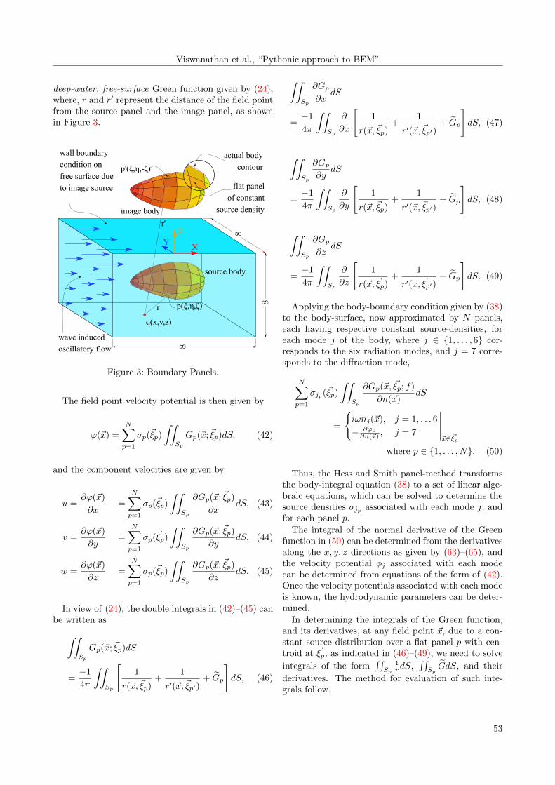
deep-water, free-surface Green function given by (24),where, r and r′ represent the distance of the field pointfrom the source panel and the image panel, as shownin Figure 3.

p(ξ,η,ζ)

p'(ξ,η,-ζ)

wave induced

oscillatory flow

flat panel

of constant

source density

actual body

contour

wall boundary

condition on

free surface due

to image source

q(x,y,z)

image body

source body

r'

r

∞

∞

∞

X

ZY

Figure 3: Boundary Panels.

The field point velocity potential is then given by

ϕ(~x) =

N∑p=1

σp(~ξp)

∫∫Sp

Gp(~x; ~ξp)dS, (42)

and the component velocities are given by

u =∂ϕ(~x)

∂x=

N∑p=1

σp(~ξp)

∫∫Sp

∂Gp(~x; ~ξp)

∂xdS, (43)

v =∂ϕ(~x)

∂y=

N∑p=1

σp(~ξp)

∫∫Sp

∂Gp(~x; ~ξp)

∂ydS, (44)

w =∂ϕ(~x)

∂z=

N∑p=1

σp(~ξp)

∫∫Sp

∂Gp(~x; ~ξp)

∂zdS. (45)

In view of (24), the double integrals in (42)–(45) canbe written as∫∫

Sp

Gp(~x; ~ξp)dS

=−1

4π

∫∫Sp

[1

r(~x, ~ξp)+

1

r′(~x, ~ξp′)+ Gp

]dS, (46)

∫∫Sp

∂Gp∂x

dS

=−1

4π

∫∫Sp

∂

∂x

[1

r(~x, ~ξp)+

1

r′(~x, ~ξp′)+ Gp

]dS, (47)

∫∫Sp

∂Gp∂y

dS

=−1

4π

∫∫Sp

∂

∂y

[1

r(~x, ~ξp)+

1

r′(~x, ~ξp′)+ Gp

]dS, (48)

∫∫Sp

∂Gp∂z

dS

=−1

4π

∫∫Sp

∂

∂z

[1

r(~x, ~ξp)+

1

r′(~x, ~ξp′)+ Gp

]dS. (49)

Applying the body-boundary condition given by (38)to the body-surface, now approximated by N panels,each having respective constant source-densities, foreach mode j of the body, where j ∈ {1, . . . , 6} cor-responds to the six radiation modes, and j = 7 corre-sponds to the diffraction mode,

N∑p=1

σjp(~ξp)

∫∫Sp

∂Gp(~x, ~ξp; f)

∂n(~x)dS

=

{iωnj(~x), j = 1, . . . 6

− ∂ϕ0

∂n(~x) , j = 7

∣∣∣∣∣~x∈ ~ξp

where p ∈ {1, . . . , N}. (50)

Thus, the Hess and Smith panel-method transformsthe body-integral equation (38) to a set of linear alge-braic equations, which can be solved to determine thesource densities σjp associated with each mode j, andfor each panel p.

The integral of the normal derivative of the Greenfunction in (50) can be determined from the derivativesalong the x, y, z directions as given by (63)–(65), andthe velocity potential φj associated with each modecan be determined from equations of the form of (42).Once the velocity potentials associated with each modeis known, the hydrodynamic parameters can be deter-mined.

In determining the integrals of the Green function,and its derivatives, at any field point ~x, due to a con-stant source distribution over a flat panel p with cen-troid at ~ξp, as indicated in (46)–(49), we need to solve

integrals of the form∫∫Sp

1rdS,

∫∫SpGdS, and their

derivatives. The method for evaluation of such inte-grals follow.

53


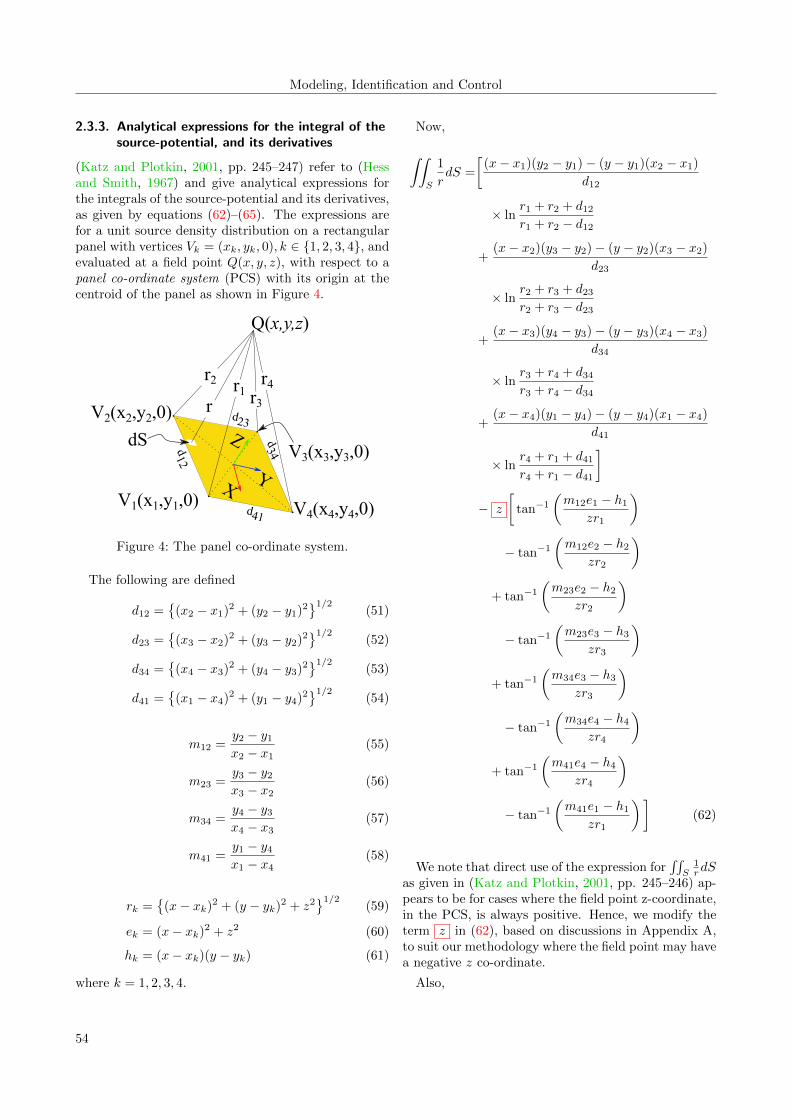
2.3.3. Analytical expressions for the integral of thesource-potential, and its derivatives

(Katz and Plotkin, 2001, pp. 245–247) refer to (Hessand Smith, 1967) and give analytical expressions forthe integrals of the source-potential and its derivatives,as given by equations (62)–(65). The expressions arefor a unit source density distribution on a rectangularpanel with vertices Vk = (xk, yk, 0), k ∈ {1, 2, 3, 4}, andevaluated at a field point Q(x, y, z), with respect to apanel co-ordinate system (PCS) with its origin at thecentroid of the panel as shown in Figure 4.

Z

XY

V4(x4,y4,0)V1(x1,y1,0)

V2(x2,y2,0)

V3(x3,y3,0)d12

d23

d34

d41

Q(x,y,z)

rr1 r3r4

dS

r2

Figure 4: The panel co-ordinate system.

The following are defined

d12 ={

(x2 − x1)2 + (y2 − y1)2}1/2

(51)

d23 ={

(x3 − x2)2 + (y3 − y2)2}1/2

(52)

d34 ={

(x4 − x3)2 + (y4 − y3)2}1/2

(53)

d41 ={

(x1 − x4)2 + (y1 − y4)2}1/2

(54)

m12 =y2 − y1

x2 − x1(55)

m23 =y3 − y2

x3 − x2(56)

m34 =y4 − y3

x4 − x3(57)

m41 =y1 − y4

x1 − x4(58)

rk ={

(x− xk)2 + (y − yk)2 + z2}1/2

(59)

ek = (x− xk)2 + z2 (60)

hk = (x− xk)(y − yk) (61)

where k = 1, 2, 3, 4.

Now,

∫∫S

1

rdS =

[(x− x1)(y2 − y1)− (y − y1)(x2 − x1)

d12

× lnr1 + r2 + d12

r1 + r2 − d12

+(x− x2)(y3 − y2)− (y − y2)(x3 − x2)

d23

× lnr2 + r3 + d23

r2 + r3 − d23

+(x− x3)(y4 − y3)− (y − y3)(x4 − x3)

d34

× lnr3 + r4 + d34

r3 + r4 − d34

+(x− x4)(y1 − y4)− (y − y4)(x1 − x4)

d41

× lnr4 + r1 + d41

r4 + r1 − d41

]

− z

[tan−1

(m12e1 − h1

zr1

)

− tan−1

(m12e2 − h2

zr2

)

+ tan−1

(m23e2 − h2

zr2

)

− tan−1

(m23e3 − h3

zr3

)

+ tan−1

(m34e3 − h3

zr3

)

− tan−1

(m34e4 − h4

zr4

)

+ tan−1

(m41e4 − h4

zr4

)

− tan−1

(m41e1 − h1

zr1

)](62)

We note that direct use of the expression for∫∫S

1rdS

as given in (Katz and Plotkin, 2001, pp. 245–246) ap-pears to be for cases where the field point z-coordinate,in the PCS, is always positive. Hence, we modify theterm z in (62), based on discussions in Appendix A,to suit our methodology where the field point may havea negative z co-ordinate.

Also,

54


∫∫S

∂

∂x

(1

r

)dS =

[y1 − y2

d12lnr1 + r2 − d12

r1 + r2 + d12

+y2 − y3

d23lnr2 + r3 − d23

r2 + r3 + d23

+y3 − y4

d34lnr3 + r4 − d34

r3 + r4 + d34

+y4 − y1

d41lnr4 + r1 − d41

r4 + r1 + d41

](63)

∫∫S

∂

∂y

(1

r

)dS =

[x1 − x2

d12lnr1 + r2 − d12

r1 + r2 + d12

+x2 − x3

d23lnr2 + r3 − d23

r2 + r3 + d23

+x3 − x4

d34lnr3 + r4 − d34

r3 + r4 + d34

+x4 − x1

d41lnr4 + r1 − d41

r4 + r1 + d41

](64)

∫∫S

∂

∂z

(1

r

)dS =

[tan−1

(m12e1 − h1

zr1

)

− tan−1

(m12e2 − h2

zr2

)

+ tan−1

(m23e2 − h2

zr2

)

− tan−1

(m23e3 − h3

zr3

)

+ tan−1

(m34e3 − h3

zr3

)

− tan−1

(m34e4 − h4

zr4

)

+ tan−1

(m41e4 − h4

zr4

)

− tan−1

(m41e1 − h1

zr1

)](65)

It is noted that the values given by (63) and (64)become infinite when the field point is on the elementedges, and go to zero when the field point is at thecentroid (Katz and Plotkin, 2001, p. 247). This is nota problem in the present development, as the compu-tation at the singular field points are not used.

The value given by (65) is singular at the centroidand tends to ∓2π, depending on the direction of ap-proach towards z = 0. I.e., the normal velocity inducedby a source panel at its centroid is +σ

2 on the positive

side, and −σ2 on the negative side. This accounts for

the limiting procedure described in the formulation of(40).

We avoid this singularity by considering the sourcepanels s to lie at an infinitesimal distance below thebody panels p as shown in Figure 5 (Guha, 2012). Thepoint where the body boundary condition is to be sat-isfied now lies at the centroid of the body panel, at avery small distance from the source panel, and thus thesingularity is avoided in the calculations based on (65).

Actual bodycontour

Edges of flatbody panels approximatingthe body surface

Source panelslying belowbody panels

body panelnull point

collocationdistance

Figure 5: Source panels beneath body panels.

2.3.4. Numerical evaluation of the integrals of thewavy Green function, and its derivatives

The wavy part of the Green function, Gp, and itsderivatives along the x, y, and z directions, can beevaluated using the GRADIF subroutine of Telste andNoblesse (1986), as discussed in Sec. 2.2.2. To imple-ment the GRADIF subroutine in our PYTHON code,we reconstruct the subroutine in FORTRAN and wrapit to PYTHON as discussed in Sec. 3.2 and 3.2.4.

In evaluating the integrals of the wavy part of theGreen function, and of its derivatives, we make use ofthe consideration that these terms are regular through-out the fluid domain and vary spatially with the wavelength, which is generally large compared to the di-mension of the immersed surface panel. Hence, G and∂G/∂n can be considered constant over a panel, and avalid approximation to the integral is to evaluate theintegrands at the centroid of a panel and multiply it bythe associated panel area. See (McTaggart, 2002, Sec.5.3), and Guha and Falzarano (2013). Thus,∫∫

Sp

GpdS = Gp∆Sp (66)∫∫Sp

∂Gp∂~x

dS =∂Gp∂~x

∆Sp, ~x = xı+ y+ zk, (67)

where ∆Sp is the surface area of panel p.

55


2.3.5. Determination of the source densities – Theα matrix

When the expressions for the Green function have beencomputed, the next step is to compute the source den-sities. To this end, let α be an N × N matrix whereeach term αps represents the induced normal velocityat the centroid of body panel p, p ∈ {1, . . . , N}, dueto unit source density distributions on source panel s,s ∈ {1, . . . , N}. In the presence of a free surface, thisterm would also include the induced normal velocity atthe body panel centroids due to the image of the sourcepanels about the free surface. In addition, if there is awave present on the free surface, then this term wouldalso include the integral of the normal derivative of thewavy part of the Green function due to an oscillatingsource of unit magnitude on the source panel s, oscil-lating at a frequency equal to the wave frequency ω.Application of the body boundary condition (7) yields

αω11 αω12 . . . αω1Nαω21 αω22 . . . αω2N

......

......

αωN1 αωN2 . . . αωNN

σωj1σωj2...

σωjN

=

vn,ωj1vn,ωj2

...vn,ωjN

(68)

where, with reference to (7), vn,ωjp , p ∈ {1, . . . , N} is

given by iωnj for j ∈ {1, . . . , 6} and−∂ϕω

0

∂n for j = 7,evaluated at the centroid (xp, yp, zp) of panel p. Herenj is given by (8), and (9).

Thus, (68) is the integral equation (40) expressed asa set of algebraic equations in the matrix form. Thesource density distribution associated with each panels for the jth mode, corresponding to the frequency ω,σωjs , may now be determined from (68).

2.3.6. Determination of the velocity potentials –The β matrix

Next, the velocity potentials are computed. Let βbe an N × N matrix where each term βωps repre-sents the velocity potential at the centroid of panelp, p ∈ {1, . . . , N}, due to unit source distributions oneach panel s, s ∈ {1, . . . , N}, subject to the same con-ditions as above for the presence of a free surface, andwaves on the free surface. Then, we have

ϕωj1ϕωj2

...ϕωjN

=

βω11 βω12 . . . βω1Nβω21 βω22 . . . βω2N

......

......

βωN1 βωN2 . . . βωNN

σωj1σωj2...

σωjN

. (69)

We note that (69) is the matrix equivalent of the setof algebraic equations representing the integral equa-tion (37) when evaluated at the panel centroids. Thesolution of (69) gives the velocity potentials ϕωjp for

j ∈ 1, . . . , 7, for each incident wave frequency ω, eval-uated at the centroid of each panel p.

2.3.7. Determination of the Froude–Kryloff anddiffraction loads

Having determined the diffraction potentials ϕω7pfrom

(69), the excitation force along any DoF k, for any inci-dent frequency ω may now be expressed with referenceto (16) as

F ek (ω, t) =

[−iωρ

N∑p=1

{ϕω0p

+ ϕω7p

}nkp∆Sp

]eiωt.

(70)

Here, nkp is the kth component of the generalized unitnormal vector given by (8), and (9), evaluated at thecentroid of body panel p, and ∆Sp is the area of bodypanel p.

2.3.8. Determination of the radiation loads

Having determined the radiation potentials ϕωjp from

(69), the added-mass and damping loads along the kth

DoF due to body oscillation along the jth DoF withfrequency ω, can now be expressed with reference to(19) as

Aωkj = − ρω

N∑p=1

I{ϕωjp

}nkp∆Sp (71)

Bωkj = −ρN∑p=1

R{ϕωjp

}nkp∆Sp. (72)

Here, j, k ∈ {1, . . . , 6}, nkp is the kth component ofthe generalized unit normal vector given by (8), and(9), evaluated at the centroid of body panel p, j is theradiation mode of the body, and ∆Sp is the area ofbody panel p.

3. Computer Implementation

3.1. The aims

To develop a methodology for computer implementa-tion of the panel method, we list out the desired resultsfrom the implementation:

• body visualization.

• mean free surface visualization.

• image body visualization in case of the presenceof a free surface.

• visualization of panel diagonals and normals tocheck correct orientation of panels.

56


• field point velocities along the xy and xz planesfor visualization of the effects of the source part,image part, and wavy part of the Green function.

• graphical representation of the source density dis-tribution associated with each panel.

• determine added-mass, damping and excitationforces for specified degrees of freedom.

• output storage as a .txt file with simulation pa-rameters specified for identification.

• graphical representation of specific hydrodynamicresults from the results stored in the .txt file, andgeneration of .csv files to enable presentation ofresults in a LATEX document or similar environ-ment.

3.2. The implementation

From the flow-chart shown in Figure 6, we note thatthe implementation has the following structure:

SFI OMHyD V0R1 : The file containing the belowlisted code components.

3D Diffraction.py : The front end PYTHON codewhere the analysis parametersand options are specified.

diff 3d obj func.py : The PYTHON code containingthe various functions used incarrying out the analysis.

Hyd mstr( ): The master function which in-terfaces the other miscellaneousfunctions and solves the varioussub-problems.

gradif... .pyd : A dynamic link library thatcontains a PYTHON module,or set of modules, to be calledby other PYTHON code. Inthis case, the wrapped FOR-TRAN code for the infinitedepth Green function.

libgradif... .dll : Additional .dll files generatedduring the wrapping of FOR-TRAN code.

am.txt : The text file that contains theresults of the analysis.

Plotter.py : PYTHON code for generatingplots of the outputs stored inthe generated text file.

plt file.csv : The comma separated value filefor easy plotting of hydrody-namic parameters in LATEX orsimilar package.

The description of the implementation is given be-low.

3.2.1. Plotting the body, free surface, imagebody,determination of panel parameters, andcalculation of hydrostatics

The environment, body, panel, DoF, and plot param-eters are to be specified in the 3D Diffraction.py,which is the front-end of the code. Details of inputsare indicated by comments in the code.

The above parameters are passed on as arguments tothe function Hyd mstr.py, which is present inside thefile diff 3d obj func.py, and a message is displayedin the shell indicating this transfer.

The unit conversion of the user-defined data to unitsfor use during computations is performed, e.g., thewave direction is specified in degrees by the user, andthis is converted to radians for use in the code.

The next step is to check if the type of body specifiedby the user is defined in the code. An error message isdisplayed if the body type is not defined, and the pro-gram execution is terminated. This step is not shownin the flow-chart.

If the body type is defined, then the next step is toset the plot definitions for displaying the body and thefree surface, if any.

This is followed by a block of code to mitigate con-flicting scenarios, as described by the comments in thecode. This step is not shown in the flow chart.

The next step is to determine the parameters forplotting the body, image, and free surface as required.It is effected by calling the function cube param. De-tails of the arguments passed, and values returned canbe found in the code comments. To summarize, thisfunction takes the passed arguments and generates pa-rameters for plotting (i) the body, and the completeimage body, in the case of a submerged body, in thepresence of a free surface, (ii) the body surface, exclud-ing the top surface, and image of all surfaces except thetop surface, for a floating body, and (iii) only the body,if there is no free-surface.

The next step is the plotting of the body/image/freesurface based on the return values from the previousstep. This is effected by a call to the plt cube func-tion which contains the PYTHON code for plotting therequired surfaces.

Once this stage of execution is reached, a progressmessage is displayed in the shell window. This is notdepicted in the flow chart.

57


Call Hydrodynamics master-functionStart Specify environmental, body, panel, DoF, plot parameters Stop

Determine the sourcedensities

Determine the panelnull point velocitiesand plot

Fn. field_point_velPlot field point velocities

Display graphical output

Open data fileStart Stop

Fn

. : w

av_g

reen

-fun

c

Fn

. : g

radi

fF

2PY

In

terf

ace

Plot the required dimensional or non dimensional values andwrite the .csv file

Plot definitions

Fn. : cube_param

Fn. : plt_cube

Fn. : pan_vert_cub

Determine body parametersfor plotting

Plot body, image body, and free surface as required

Determine vertex coordinatesof body panels

Determine panel parameterslike diagonals, normals, etc. Fn. : panel_par

Plot panel diagonals? Fn. : plt_diag

Determine panel-based hydrostatics Fn. : hydrostatics

Determine non-wavy part of Green function

Determine the alphamatrix without wavy Green function part

Fn. : non_wav_green_func

Plot panel normals? Fn. : plt_norm

Plot collocation points? Fn. : plt_src

YES

YES

YES

Are there waves?

NO

NO

NO

NO

Determine generalized normalsfor each panel

Determine wavy part of GreenFunction for each frequency

Determine Alpha (α) and Beta (β) matrices for each frequency

Determine normal velocities at panel centroids correspoinding to

radiation mode

Determine source densities of panels correspoinding to radiation mode

Determine corresponding radiation potentials

Determine corresponding added mass and damping values

Determine corresponding wave number

Determine corrresponding incidentpotential

Determine normal derivatives of the incident potential at panel centroids

Determine the source densities corresponding to the diffraction potential

Determine the diffraction potential

Determine the excitation forces

Write the output file

YES

Return to caller( ).txtS

FI_

OM

HyD

_V0R

1

3D_Diffraction.py

dif

f_3d

_ob

j_fu

nc.

py

dif

f_3d

_ob

j_fu

nc.

py

Hyd

_mst

r( )

Plotter.py

Plot field point data?

Plot source density?

Plot source density

Fn. : src_str

NO

YES

YES

NO

.csv

Figure 6: Implementation flow chart.

58


The next step is to determine the panel vertices ofthe source and image body. The order of storage of thepanel vertices is important in the view of determiningthe diagonals and the surface normals. This is effectedby calling the function pan vert cub. The process iseasily understood from the code comments. The re-turn values are vectors ‘vert’, ‘verti’, ‘z bp’, and ‘z tp’,which contains the vertex coordinates of the body pan-els, the image panels, the z-coordinate of the bottomsurface, and the z-coordinate of the top surface, respec-tively.

The next step is the determination and storage ofpanel parameters as described below.

If the coordinates of the four vertices of a quadri-lateral panel are Vi(xi, yi, zi), i ∈ {1, . . . , 4}, then the

diagonals ~D1 and ~D2 are given as

~D1 = ~V3 − ~V1 = (x3 − x1)ı+ (y3 − y1)+ (z3 − z1)k(73)

~D2 = ~V4 − ~V2 = (x4 − x2)ı+ (y4 − y2)+ (z4 − z2)k.(74)

Here, ı, , k are unit vectors along x, y and z directions.The normal ~n and the unit normal n to the panel

are then given as

~n = ~D1 × ~D2 (75)

n =~n

|n|= n1 ı+ n2+ n3k, (76)

where n1, n2, and n3 are the x, y and z components ofthe unit surface normal.

Similarly, defining ~L lying on the surface of the panelas

~L =

[x4 + x3

2− x1 + x2

2

]ı

+

[y4 + y3

2− y1 + y2

2

]

+

[z4 + z3

2− z1 + z2

2

]k. (77)

The unit vector along ~L is

l =~L

|~L|= l1 ı+ l2+ l3k. (78)

Another vector lying on the surface of the panel andperpendicular to both l and n would then be given by

~P = n× l. (79)

The unit vector along ~P is given as,

p =~P

|~P |= p1i+ p2j + p3k. (80)

The postion vector of the centroid of the panel is

~C = cx ı+ cy + cz k, (81)

where

cx =cx1d1 + cx2d2 + cx3d3 + cx4d4

d1 + d2 + d3 + d4,

cy =cy1d1 + cy2d2 + cy3d3 + cy4d4

d1 + d2 + d3 + d4,

cz =cz1d1 + cz2d2 + cz3d3 + cz4d4

d1 + d2 + d3 + d4. (82)

cx1 =x1 + x2

2, cx2 =

x2 + x3

2, cx3 =

x3 + x4

2, cx4 =

x4 + x1

2,

cy1 =y1 + y2

2, cy2 =

y2 + y32

, cy3 =y3 + y4

2, cy4 =

y4 + y12

,

cz1 =z1 + z2

2, cz2 =

z2 + z32

, cz3 =z3 + z4

2, cz4 =

z4 + z12

.

(83)

and

d1 =√

(x2 − x1)2 + (y2 − y1)2 + (z2 − z1)2,

d2 =√

(x3 − x2)2 + (y3 − y2)2 + (z3 − z2)2,

d3 =√

(x4 − x3)2 + (y4 − y3)2 + (z4 − z3)2,

d4 =√

(x1 − x4)2 + (y1 − y4)2 + (z1 − z4)2. (84)

The panel coordinates (xi, yi, zi), i ∈ {1, . . . , 4}, canbe transformed from the body coordinate system de-fined by (ı, , k) to the local coordinate system defined

by (l, p, n) as (xli, yli, 0), i ∈ {1, . . . , 4}, using

xli = (xi − cx)l1 + (yi − cy)l2 + (zi − cz)l3,yli = (xi − cx)p1 + (yi − cy)p2 + (zi − cz)p3. (85)

The centroid of the source panel (cxp , cyp, c

zp), lying

at a distance specified by parameter cp from the bodypanel, is given by

cxp = cx − cp · n1, cyp = cy − cp · n2, c

zp = cz − cp · n3

(86)

The panel parameters calculated above for eachsource and image panel are stored as a vector of vectorsfor use in later calculations. Details of the storage canbe understood from the code.

If the diagonals, normals and centroids of the sourcepanels are required to be plotted, functions plt diag,plt norm, and plt src are called.

The function hydrostatics determines the hydro-static parameters of the body as described below.

The area of a quadrilateral panel, given its four ver-tices, is

A =1

2

{(x1y2 + x2y3 + x3y4 + x4y1)

− (x2y1 + x3y2 + x4y3 + x1y4)}. (87)

59


Thus, the volume bounded by N panels is given by

∇ =

N∑j=1

Ajn3,jzj . (88)

Here, n3,j is the z component of the unit normal topanel j, and zj is the z-coordinate of the centroid ofpanel j.

The vertical and longitudinal centres of buoyancy aregiven by

zCB =12

∑Nj=1Ajn3,jz

2j

∇, (89)

xCB =12

∑Nj=1Ajn3,jzjxj

∇. (90)

Here, xj is the x -coordinate of the centroid of panel j.The longitudinal centre of flotation is given as

xWP =−∑Nj=1Ajn3,jxj

AWP, (91)

where AWP is the waterplane area given by

AWP = −N∑j=1

Ajn3,j . (92)

The moment of the waterplane about the x and yaxes are given by

IxxWP = −N∑j=1

Ajn3,jy2j , (93)

IyyWP = −N∑j=1

Ajn3,jx2j . (94)

The hydrostatic stiffness terms are then given by

C33 = ρgAWP (95)

C35 = −ρgAWPxWP (96)

C44 = ρg {∇zCB −∇zCG + IxxWP} (97)

C53 = C35 (98)

C55 = ρg {∇zCB −∇zCG + IyyWP} . (99)

They may be non-dimensionalized as

Cnd33 =

C33

ρgL2nd

, (100)

Cnd35 =

C35

ρgL3nd

, (101)

Cnd44 =

C44

ρgL4nd

, (102)

Cnd53 = Cnd

35 , (103)

Cnd55 =

C55

ρgL4nd

, (104)

where Lnd is the characteristic length. This is simi-lar to the non-dimensionalization in WAMIT (Newmanand Lee, 2013, Sec. 3.1).

Once the hydrostatics are determined, they are dis-played in the shell output along with a progress mes-sage.

3.2.2. The source, and image-source Greenfunctions

The next step is to determine the non-wavy part(s)of the Green function at the body panel centroidsdue to unit source distribution on the source pan-els/image panels. This is effected by calling the func-tion non wav green func, which returns the follow-ing:

The IV matrix: An N × N matrix, each element ofwhich represents the induced velocity at the cen-troid of panel p, by unit source density distribu-tion on source panel s. Each element ivps is itselfa vector [vxps, v

yps, v

zps], which represents the x, y, z

components of the induced velocity.

The IVI matrix: An N × N matrix, each element ofwhich represents the induced velocity at the cen-troid of panel p by unit source density distribu-tion on image of source panel s, referred to aspanel s′. Each element ivips′ is itself a vector[vxps′ , v

yps′ , v

zps′ ], which represents the x, y, z com-

ponents of the induced velocity.

The DNR matrix: An N ×N matrix, each element ofwhich represents the normal component of the in-duced velocity at the centroid of panel p by unitsource density distribution on source panel s.

The DNRI matrix: An N × N matrix, each elementof which represents the normal component of theinduced velocity at the centroid of panel p byunit source density distribution on image of sourcepanel s, referred to as panel s′.

The R INV matrix an N × N matrix, each elementof which represents the induced velocity potentialat the centroid of panel p by unit source densitydistribution on source panel s.

The RI INV matrix an N × N matrix, each elementof which represents the induced velocity potentialat the centroid of panel p by unit source densitydistribution on image of source panel s, referredto as panel s′.

In determining the IV and IVI matrices, we makeuse of (63), (64), and (65).

60


In determining the DNR and DNRI matrices, wemake use of the relation

vnps = ~vps · np, (105)

where vnps is the induced normal velocity at the cen-troid of panel p due to source density distribution onpanel s. ~vps = vxps ı+vyps+vzpsk is the induced velocityvector at the centroid of panel p due to source den-sity distribution on panel s, and np is the unit positivesurface normal at the centroid of panel p given by (76).

In determining the R INV and RI INV matrices,we make use of (62).

3.2.3. Body in steady, uniform incident flow

In the presence of an incident flow, assuming the bodyto be fixed, the problem to be solved is a diffractionproblem, and hence the mode j = 7 for (68). Eachterm αps of the α matrix represents the induced normalvelocity at the centroid of the pth body panel due tounit source density distribution on the sth source panel,and on the s′ th image-source panel in addition, if thereis a free surface . Thus, each term αps is given as

αps =−1

4π

[ ∫∫S

∂

∂n(~ξp)

{1

r(~ξp, ~ξs)

}dS

+

∫∫S′

∂

∂n(~ξp)

{1

r′(~ξp, ~ξs′)

}dS

]. (106)

Here, p, s, s′ ∈ {1, . . . , N}.With reference to the definition of the DNR, and

DNRI matrices, the α matrix can be expressed as

α = DNR + DNRI (107)

Once the α matrix is determined, the source densitydistribution associated with each panel may now bedetermined as

[σ7s]T = [αps]

−1[vn7p]T; p, s ∈ {1, . . . , N} (108)

Here, in the sole presence of an incident flow definedby ~v∞ = [vx∞, v

y∞, v

z∞], vn7p

is the negative of the com-ponent of the incident flow velocity in the direction ofthe positive surface normal of the pth panel, as givenin the description of (68), and is expressed as

vn7p= −~v∞ · np. (109)

Here, ~v∞ is specified in the inputs, and np is deter-mined using (76).

Once the density distribution associated with eachsource panel is determined, the null point velocities atthe panel centroids may be determined as

[Vp]T = [IVps][σ7s

]T + [IVIps′ ][σ7s]T. (110)

These are then summed up with the incident flow atthe centroid of each panel and plotted as a quiver plot.

3.2.4. Body in the presence of free-surface waves

If waves are present, and the body is free to move alongthe specified DoFs, then the diffraction-radiation prob-lem is to be solved.

We start by determining the generalized normalsgiven by (8) and (9).

The presence of waves necessitates theevaluation of the integral of the wavy partof the Green function and its derivatives.This is accomplished by calling the functionwav green func, which returns, for each wavefrequency specified in the input:

The SG0 matrix: An N × N matrix, each element ofwhich represents the integral of the wavy part ofthe Green function at the centroid of panel p dueto an oscillating unit density source distributionon panel s, calculated based on (25) and (66).

The SDG0 N matrix: An N × N matrix, each ele-ment of which represents the integral of the normalderivative of the wavy part of the Green functionat the centroid of panel p due to an oscillating unitdensity source distribution on panel s, calculatedbased on (32)–(34), (67), and (105).

In determining the R0(h, v) and R1(h, v) in (32)–(34), we make use of the gradif function which is orig-inally written in FORTRAN, the printout of which, isgiven as an appendix to (Telste and Noblesse, 1986).We use F2PY (Peterson, 2005) to wrap the FOR-TRAN code for PYTHON. This wrapping generatesthe gradif... .pyd and the libgradif... .dll

files in Windows OS. Instead of .dll files, .so files aregenerated by F2PY on Linux/Mac OS. The gradiffunction may now be called into PYTHON, as anyother regular PYTHON function.

With reference to (68), the α matrix correspondingto wave frequency ω is now defined as matrix αω, whereeach element αωps represents the normal component ofthe induced velocity at the centroid of body panel pdue to

1. unit source density distribution on source panel s,and,

2. unit source density distribution on the image ofsource panel s, referred to as s′, in case of thepresence of a free surface, and,

3. oscillating source density distribution of unit mag-nitude on panel s.

61


Thus, the elements of the αω matrix are given by

αωps =−1

4π

[ ∫∫S

∂

∂n(~ξp)

(1

r(~ξp, ~ξs)

)dS

+

∫∫S′

∂

∂n(~ξp)

(1

r′(~ξp, ~ξs′)

)dS

]

+

∫∫S

∂G(~ξp, ~ξs; f)

∂n(~ξp)dS, (111)

where p, s, s′ ∈ {1, . . . , N}.With reference to the definitions of the DNR,

DNRI, and the SDG0 N matrices, we see that

αω = DNR + DNRI + SDG0 Nω (112)

Again, in determining the normal components fromthe (x, y, z) components given by (43), (44), (45), and(67), we make use of (105).

Once the α matrix is determined, we may determinethe source density distribution σωjs associated with eachsource panel s, for a given frequency of oscillation ω,for a given mode of oscillation j from equations of theform of (108), with vn,ωjp ’s corresponding to the nor-mal velocity at the panel centroids due to oscillationswith unit amplitude corresponding to each mode j, asindicated by (7), (8), and (9). Thus,

[σωjs ]T = [αωps]−1[vn,ωjp ]T (113)

With reference to (69), the β matrix correspond-ing to wave frequency ω, is now defined as matrix βω

where each element βωps represents the induced velocitypotential at the centroid of body panel p due to

1. unit source density distribution on source panel s,and,

2. unit source density distribution on image of sourcepanel s, referred to as s′, in case of the presenceof a free surface, and,

3. oscillating source density distribution of unit mag-nitude on panel s.

Thus, the elements of the βω matrix are given by

βωps =−1

4π

[ ∫∫S

(1

r(~ξp, ~ξs)

)dS

+

∫∫S′

(1

r′(~ξp, ~ξs′)

)dS

]+

∫∫S

G(~ξp, ~ξs; f)dS, (114)

where p, s, s′ ∈ {1, . . . , N}.

With reference to the definitions of the R INV,RI INV, and the SG0 matrices, we see that

βω = R INV + RI INV + SG0ω. (115)

The complex spatial component of the velocity po-tential at the centroid of body panel p, correspondingto the jth mode, with frequency ω, can now be ex-pressed, with reference to (69), as

[ϕωjp ]T = [βωps][σωjs ]T. (116)

Once the radiation potentials are known, the corre-sponding added mass and damping components in thekth DoF, due to body motion along the jth DoF, canbe determined by using (71) and (72).

Mode j = 7 in this case, is the diffraction problemwith the body held fixed at its mean position in inci-dent waves of specified frequencies.

With reference to (68),

vn,ω7p= − ∂

∂n(ϕω0 )

∣∣∣∣~ξp

(117)

Where ϕω0 is the velocity potential given by (2),~ξp(ξp, ηp, ζp) is the centroid of submerged body panelp.

The wave induced water-particle velocity at the cen-troid of the pth panel is indicated by ~u0p(u0p , v0p , w0p),where

u0p=

∂

∂x

(ϕω0p

)∣∣∣∣~ξp

= Zaω cos γe−ik(ξp cos γ−ηp sin γ)ekζp (118)

v0p=

∂

∂y

(ϕω0p

)∣∣∣∣~ξp

= Zaω sin γe−ik(ξp cos γ−yηp sin γ)ekζp (119)

w0p==

∂

∂z

(ϕω0p

)∣∣∣∣~ξp

= iZaωe−ik(ξp cos γ−ηp sin γ)ekζp . (120)

Here, γ [rad] is the wave direction, and Za = 1 m isthe wave amplitude. See, (Guha, 2012, pp. 31–32).

Also, with reference to (105),

vn,w7p= −~u0p · np, (121)

where np is the unit outward normal to the pth bodypanel given by (76).

The α matrix being given by (112), an equationof the form (108) may now be solved to determinethe source densities σω7s

corresponding to each incidentwave frequency ω.

62


The matrix of diffraction potentials[ϕω7p

]associated

with each body panel p, for each incident wave fre-quency ω, is obtained from a relation similar to (116).

The excitation force along any DoF, k, may now bedetermined with reference to (16) as

F ek = −iωρN∑p=1

(ϕ0p

+ ϕ7p

)nkp∆Sp. (122)

The added-mass, damping and excitation force ma-trices are now written to an output file am.txt,along with identification details, and placed inside theSFI OMHyD folder.

If field point velocities are to be plotted, the functionfield point vel is called. This function calculates thefield point velocities in a similar manner to the calcu-lation of the body panel null point velocities describedearlier. The only difference being that the IV andIVI matrices are determined for the field points andsource/image panels, in this case.

In plotting the field velocities to illustrate the effectof the radiated waves, only the IV matrix is considered,since the effect of the image source is inherent in thecalculation of the source strengths corresponding to theradiation modes.

If source densities associated with each panel are tobe displayed, they are plotted as colormapped spheresat the body panel centroids by calling the functionsrc str.

A separate post processing code Plotter.py enablesthe user to generate required plots of data containedwithin the .txt file. The code has options to spec-ify the k, j components of the added-mass and damp-ing terms, as given by (20) and (21), to be plotted.The plot for the excitation force in the kth directionis also generated. Options are also available to plotdimensional as well as non dimensional values. In ad-dition to this, the code also generates a .csv file forthe data contained in the generated plots to make itreadily available for use in LATEXdocuments by usingthe pgfplots package.

4. Results

We endeavour to discuss the results generated using theOMHyD code, as far as possible, by using the screen-shot of the graphical output as obtained. Whereverpossible, we compare OMHyD and ANSYS-AQWA re-sults.

The OMHyD files are available for download atgithub.com/Savin-Viswanathan/OMHyD-PA.

The required parameters for the various cases pre-sented are specified in the front-end files identified by

the figure number in this paper. Thus, for each casepresented, there is a different front-end file availablein the download, but they all use the same functionscontained inside the file named diff 3d obj func.py.More instructions on how to run the different scenariosare given in the README.txt file of the download.

For better comprehension of some of the scenarios,it is recommended to run the corresponding front-endcode to get the three-dimensional graphical output.

4.1. Plotting the body and image panels

Figure 7a shows the body panels generated by the codefor a cubical body of side 10 m discretized into squarepanels of side 5 m, while Figure 7b shows the normalsand diagonals of the body panels. The indication of thesurface normals and diagonals helps us in ascertainingthat the vertices are stored in the required order duringthe function call pan vert cub.

If the free surface is present, the effect of the imagepanels are also to be considered in the determinationof the Green function. Hence, for a submerged body,in the presence of a free surface, the plot is as shownin Figure 8a. The image body is represented by thegrey dashed lines, and the free surface by the red gridat z = 0. The diagonals and normals are not shownto avoid cluttering the image. However, these may beswitched on, if required. In this case the body hasdimensions 10× 10× 5 m and the panel side is 2.5 m.

If the body is floating, then the top surface of thebody, and the image of the top surface need not beplotted as is shown in Figure 8b.

4.2. Body in infinite fluid in the presenceof a steady uniform flow: Effect ofthe free-space Green function

Consider a cube of side 10 m, in an unbounded fluid,in the presence of a steady flow along the positive Xaxis given by vf = [1, 0, 0] m/s. The free space Greenfunction is applicable, and is given by G∗ = −1

4πr . Con-sider a field point lying at a distance, greater than thelength of the panel side, from the body. The velocitypotential of this field point may now be expressed asthe sum of the incident velocity potential and the veloc-ity potential due to source density distributions on thequadrilateral panels discretizing the body surface. Theinability to plot velocities at field points lying closer tothe body surface is due to the fact that the velocity po-tential increases as one approaches the element edgesand goes to infinity at the edge, as indicated by (62).The induced velocities at the body panel centroids canalso be determined and plotted. The graphical outputfrom the code showing the field point and null point ve-

63

https://github.com/Savin-Viswanathan/OMHyD-PA


x [m]

64

20

24

6

y [m]

6

4

2

0

2

4

6

z [m

]

6

4

2

0

2

4

6

(a) Body panels.

x [m]

6 4 2 0 2 4 6

y [m

]

6

4

2

0

2

4

6

z [m

]

6

4

2

0

2

4

6

(b) Panel normals and diagonals.

Figure 7: Body in infinite fluid domain.

x [m]

10.07.5

5.02.5

0.02.5

5.07.5

10.0

y [m]

10.07.5

5.02.5

0.02.5

5.07.5

10.0

z [m

]

10.0

7.5

5.0

2.5

0.0

2.5

5.0

7.5

10.0

(a) Submerged body.

x [m]

7.55.0

2.50.0

2.55.0

7.5

y [m]

7.5

5.0

2.5

0.0

2.5

5.07.5

z [m

]

7.5

5.0

2.5

0.0

2.5

5.0

7.5

(b) Floating body.

Figure 8: Body in semi-infinite fluid domain.

64


locities is shown in Figure 9. The velocities of the fluidat grid points lying only in the XY and XZ planes areshown to avoid clutter.

We observe that the presence of the body causes achange in the flow field, and it is no longer uniform.The flow diverges as it approaches the body and con-verges as it leaves the body.

The effect of a diagonal flow given by vf =[0.707, 0.707 , 0] m/s is shown in Figure 10.

The source strengths may also be indicated by a colorbar as shown in Figure 11. We notice that, on the aftpanels facing the incident flow, the source strengthsare positive since an outward flow from the panel is re-quired to oppose the incident flow and bring the totalvelocity of the fluid to zero at the panel null points,thus satisfying the boundary condition. Similarly onthe forward side, the body boundary condition impliesthe presence of a flow into the panels such that the totalfluid velocity at the null points is zero. This flow intothe panel implies the presence of a sink. This combina-tion of sources and sinks ensures the fulfillment of theconservation of mass equations in the fluid domain.The source strengths are negative on the starboard,port, bottom, and top panels, bordering the aft pan-els. This is to prevent the flow from separating fromthe body surface due to the effect of the induced ve-locity by the aft source panels. Similarly, the positivesource strengths on the starboard, port, bottom andtop panels, bordering the forward panels prevent thefluid from penetrating the body under the influence ofthe aft sink panels.

4.3. Body in semi-infinite fluid domain:Effect of the image-source Greenfunction

Consider a cuboidal body of dimensions 15 × 10 × 10m, submerged such that the top surface is 2.5 m be-low the free surface. Consider a steady, uniform flowalong the positive X axis given by vf = [1, 0, 0] m/sin the fluid domain. Since a free-surface is present,the effect of the image-body is also to be considered,and the free-surface Green function is now given byG = −1

4π

[1r + 1

r′

]. The field and null point velocities

are shown in Figure 12a.

When the immersion is such that top surface is 0.5 mbelow the water surface, the field point and null pointvelocities are as shown in Figure 12b.

When the top surface immersion depth is 2.5 m, theincident flow deviates almost symmetrically. However,when the immersion depth is 0.5 m, the flow deviationis not symmetric. This can be observed from the nullpoint velocities of the top and bottom starboard panelsbordering the aft panels, and the second and third row

x [m]

10.07.5

5.02.5

0.02.5

5.07.5

10.0

y [m]

10.0

7.5

5.0

2.5

0.0

2.5

5.0

7.5

10.0

z [m

]

10.0

7.5

5.0

2.5

0.0

2.5

5.0

7.5

10.0

(a) Field point velocities in the XY plane.

x [m]

10.07.5

5.02.5

0.02.5

5.07.5

10.0

y [m]

10.0

7.55.0

2.50.0

2.55.0

7.510.0

z [m

]

10.0

7.5

5.0

2.5

0.0

2.5

5.0

7.5

10.0

(b) Field point velocities in the XZ plane.

Figure 9: Fully submerged body in infinite fluid do-main, and in the presence of a steady uniformflow vf = [1, 0, 0] [m/s].

65


x [m]

10.07.5

5.02.5

0.02.5

5.07.5

10.0

y [m]

10.0

7.55.0

2.50.0

2.55.0

7.510.0

z [m

]

10.0

7.5

5.0

2.5

0.0

2.5

5.0

7.5

10.0

Figure 10: Fully submerged body in infinite fluid do-main, and in the presence of a steady uni-form flow vf = [0.707, 0.707, 0] m/s.

x [m]

10.07.5

5.02.5

0.02.5

5.07.5

10.0

y [m]

10.07.5

5.02.5

0.02.5

5.07.5

10.0

z [m]

10.0

7.5

5.0

2.5

0.0

2.5

5.0

7.5

10.0

2

1

0

1

2

Sour

ce st

reng

th

Figure 11: Body in infinite fluid domain: Source den-sity distribution magnitudes.

x [m]15 10 5 0 5 10 15y [m] 15105051015

z [m]

15

10

5

0

5

10

15

(a) Top surface 2.5 [m] below the free surface.

x [m]15 10 5 0 5 10 15y [m] 15105051015

z [m]

15

10

5

0

5

10

15

(b) Top surface 0.5 [m] below the free surface

Figure 12: Submerged body in semi-infinite fluid, andin the presence of a steady uniform flowvf = [1, 0, 0] m/s.

66


of field velocities from the free surface.This points to the wall condition at the free surface.

As the body moves towards the wall, the area avail-able for the flow above the body decreases, and theflow deviates to pass around the body along the otheravailable paths. An increase in the fluid velocity inthe space between the free surface and the top surfaceof the body is also observed. The function of the im-age body is to enforce this wall condition as describedin Sec. 2.2. If it were not for the image-source, thewhole of the free surface would have to be modeledwith source panels, as is done for the body.

Figure 13 shows the field and null point velocitieswhen the body is floating at a draft of 5 m. Again, weobserve that the flow near the surface does not deviatein the XZ plane but deviates in the XY plane to passaround the body.

4.4. Body in semi-infinite fluid domain inthe presence of a free surface andwaves: Effect of the wavy part of theGreen function

We consider a cuboidal body of dimensions 15×10×10m floating at a draft of 5 m. To illustrate the effect ofradiation waves, we consider the induced velocities atthe field points, due to the wavy part of the Green func-tion alone, as given by (25). The incident wave frequen-cies [rad/s] to be considered are specified by the useragainst the vector ‘omega’ in the 3D Diffraction.pyfile. We can select a particular frequency and plot theinduced velocity at the field points due to the bodyoscillating along the required DoF by specifying therequirements against parameters under the n rad freqand the Degrees of freedom fields, respectively. Tomake the velocities visible, we might need to scale thevelocities using the parameter sf rad. The image bodyis kept hidden, for aesthetic purposes.

Considering the surge motion of the body, the fieldpoint velocities are as shown in Figure 14. As the bodymoves in the positive x-direction, there is an increase inthe fluid pressure forward of the body, and a decreasein the fluid pressure aft of the body. The fluid nowcirculates around the body, from the high pressure zoneto the low pressure zone, as shown by the plots for thefield point velocities in the XY plane. Consideringthe XZ plane, we observe that low- and high-pressurezones also develop along the bottom surface.

Considering the sway motion of the body, the fieldpoint velocities are shown in Figure 15. Again, weobserve similar behaviour of the field velocities as inthe surge case.

Considering the heave motion of the body, the fieldpoint velocities are shown in Figure 16. We observe

x [m]15 10 5 0 5 10 15

y [m] 15105051015

z [m]

15

10

5

0

5

10

15

(a) Flow along the XZ plane.

x [m]

15

10

5

0

5

10

15y [m]

15

10

5

0

5

10

15

z [m]

15

10

5

0

5

10

15

(b) Flow along the XY plane.

Figure 13: Floating body in semi-infinite fluid, and inthe presence of a steady uniform flow vf =[1, 0, 0] [m/s].

67


x [m]

15

10

5

0

5

10

15

y [m]

15

10

5

0

5

10

15z

[m]

15

10

5

0

5

10

15


x [m]15 10 5 0 5 10 15

y [m]

1510

50

510

15

z [m]

15

10

5

0

5

10

15


Figure 14: Radiation waves due to surge of floatingbody.

x [m]

15

10

5

0

5

10

15

y [m]

15

10

5

0

5

10

15

z [m

]

15

10

5

0

5

10

15


x [m]

1510

50

510

15 y [m]15 10 5 0 5 10 15

z [m

]

15

10

5

0

5

10

15

(b) Field point velocities in the Y Z plane.

Figure 15: Radiation waves due to sway of floatingbody.

68


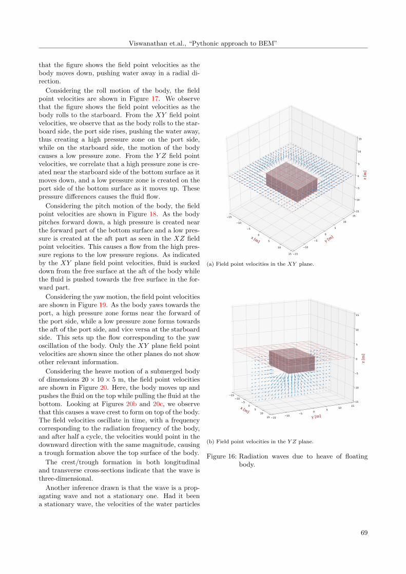
that the figure shows the field point velocities as thebody moves down, pushing water away in a radial di-rection.

Considering the roll motion of the body, the fieldpoint velocities are shown in Figure 17. We observethat the figure shows the field point velocities as thebody rolls to the starboard. From the XY field pointvelocities, we observe that as the body rolls to the star-board side, the port side rises, pushing the water away,thus creating a high pressure zone on the port side,while on the starboard side, the motion of the bodycauses a low pressure zone. From the Y Z field pointvelocities, we correlate that a high pressure zone is cre-ated near the starboard side of the bottom surface as itmoves down, and a low pressure zone is created on theport side of the bottom surface as it moves up. Thesepressure differences causes the fluid flow.

Considering the pitch motion of the body, the fieldpoint velocities are shown in Figure 18. As the bodypitches forward down, a high pressure is created nearthe forward part of the bottom surface and a low pres-sure is created at the aft part as seen in the XZ fieldpoint velocities. This causes a flow from the high pres-sure regions to the low pressure regions. As indicatedby the XY plane field point velocities, fluid is suckeddown from the free surface at the aft of the body whilethe fluid is pushed towards the free surface in the for-ward part.

Considering the yaw motion, the field point velocitiesare shown in Figure 19. As the body yaws towards theport, a high pressure zone forms near the forward ofthe port side, while a low pressure zone forms towardsthe aft of the port side, and vice versa at the starboardside. This sets up the flow corresponding to the yawoscillation of the body. Only the XY plane field pointvelocities are shown since the other planes do not showother relevant information.

Considering the heave motion of a submerged bodyof dimensions 20 × 10 × 5 m, the field point velocitiesare shown in Figure 20. Here, the body moves up andpushes the fluid on the top while pulling the fluid at thebottom. Looking at Figures 20b and 20c, we observethat this causes a wave crest to form on top of the body.The field velocities oscillate in time, with a frequencycorresponding to the radiation frequency of the body,and after half a cycle, the velocities would point in thedownward direction with the same magnitude, causinga trough formation above the top surface of the body.

The crest/trough formation in both longitudinaland transverse cross-sections indicate that the wave isthree-dimensional.

Another inference drawn is that the wave is a prop-agating wave and not a stationary one. Had it beena stationary wave, the velocities of the water particles

x [m]

15

10

5

0

5

10

15

y [m]

15

10

5

0

5

10

15

z [m

]

15

10

5

0

5

10

15


x [m]

1510

50

510

15 y [m]1510 5 0 5 10 15

z [m

]

15

10

5

0

5

10

15


Figure 16: Radiation waves due to heave of floatingbody.

69


x [m]

15

10

5

0

5

10

15y [m]

1510

50

510

15

z [m

]

15

10

5

0

5

10

15


x [m]

1510

50

510

15y [m]15 10 5 0 5 10 15

z [m

]

15

10

5

0

5

10

15


Figure 17: Radiation waves due to roll of floating body.

x [m]

15

10

5

0

5

10

15

y [m]

15

10

5

0

5

10

15

z [m]

15

10

5

0

5

10

15


x [m]15 10 5 0 5 10 15y [m]15

105

05

1015

z [m]

15

10

5

0

5

10

15


Figure 18: Radiation waves due to pitch of floatingbody.

70


x [m]

15

10

5

0

5

10

15

y [m]

15

10

5

0

5

10

15

z [m

]

15

10

5

0

5

10

15

Figure 19: Yaw induced velocities at field points lyingon the XY plane.

x [m]20 15 10 5 0 5 10 15 20y [m] 201510505101520

z [m]

20

15

10

5

0

5

10

15

20

(a) Field point velocities in the XZ plane.

x [m]

201510505101520y [m]

20 15 10 5 0 5 10 15 20

z [m

]

20

15

10

5

0

5

10

15

20

(b) Free surface field point ve-locities when viewed fromaft.

x [m]20 15 10 5 0 5 10 15 20

y [m]201510505101520

z [m

]

20

15

10

5

0

5

10

15

20

(c) Free surface field point ve-locities when viewed fromport.

Figure 20: Heave radiation of submerged body.

would have had only the vertical component.Yet another conclusion drawn is that, far away from

the body, the wave induced velocities die out.The above paragraphs, read in conjunction, indicate

the presence of circular outgoing waves with reducingamplitudes, as the wave moves away from the body.Thus, we confirm from the results that the wavy partof the Green function generates waves that satisfy theradiation condition as described by the theory in Sec.2.

These radiation waves cause a change in the hydro-dynamic pressure distribution on the body surface, andas a result, the body experiences a force which is ex-pressed mathematically by (19). The component of theforce proportional to the acceleration of the body isreferred to as the added mass, and the component pro-portional to the velocity of the body is termed as thedamping. Since both velocity and acceleration of thebody are frequency-dependent, the radiation added-mass and damping are also frequency-dependent.

4.5. The hydrodynamic coefficients of adeeply submerged cube.

Considering a deeply submerged object, we hypothe-size:

1. Since the object is submerged beyond half thewave length of the longest wave, the excitationforces must be zero.

2. There exists an associated added mass, whichmust be independent of the frequency of motionfor a deeply submerged body. This is because theextent of the volume of water which is acceleratedby the body, as is the interpretation of added massmade by Newman in (Newman, 1977), is constantin the absence of the influence of the free surface.

3. There is no associated potential damping since noradiation waves are present to carry energy awayfrom the body.

(Sarpkaya and Isaacson, 1981) gives the analyticalexpression for the translational added mass of a deeplysubmerged cube as 0.7ρa3 [kg]. Here ρ [kg/m3] is thedensity of water, and a [m] is the side of the cube.

Table 1 compares the added masses calculated by thecode to results obtained by Guha using MDLHydroDfrequency domain solver, as given in (Guha, 2012, p.60).

The results in OMHyD are for a cube of side 1 m,sea water of density 1025 kg/m3, panel size of 0.125 mgiving 384 diffracting panels, (or)panel size of 0.0625 mgiving 1536 diffracting panels, and an immersion depthof 10000 m. In MDLHydroD, 864 panels were used,

71


Table 1: Translational added-mass [kg] of a deeply sub-merged cube of side 1 m.

DoF Analytical OMHyD OMHyD GuhaPanels N/A 384 1546 864

Surge 717.50 673.29 661.68 665.37Sway 717.50 673.29 661.68 665.37Heave 717.50 673.29 661.68 665.34

while no details are given for the immersion depth andfrequencies.

The added mass, damping and excitation forces ob-tained from the code are plotted in Figure 21.

0.5 1 1.5 2 2.5 30

250

500

673.29

750

ω [rad/s]

Valu

es a33 [kg]

b33 [Ns/m]

fe3 [N]

Figure 21: Hydrodynamic coefficients of a deeply sub-merged cube (384 panels).

.

Currently, only square panels can be used inOMHyD. Use of exactly 864 panels gives erroneous re-sults. However, we see that Guha’s results with 864panels lie between our results using 384 and 1536 pan-els. We also notice that as the mesh becomes finer, theresults are diverging from the analytical value, contraryto what one would normally expect.

Sec. 2.2.1 General Modelling Requirements of theANSYS-AQWA user manual Release 14.5, 2012, re-quires the surface to be split at the water plane, andhence such an analysis seems implausible in AQWA.Further, there is no indication of the results of a panelconvergence study in (Guha, 2012), for this case.

Notwithstanding the above deficiencies, the resultspresented confirm our hypothesis above. We also ar-rive at the conclusion that our implementation of thesurface panelization, and evaluation of the integrals ofthe wavy Green function and its derivatives, are notwrong. Further proof of correctness of our procedure ispresented in sections that follow.

4.6. Panel convergence.

We look at the heave added mass, damping and excita-tion forces for a cube of side 24 [m], floating at a draftof 12 [m]. Results for discretization with square panelsof side 12, 6, 4, 3, and 2 m are shown in Figure 22.

We observe convergence when the panel side is 3 m.

PS 12 PS 6 PS 4 PS 3 PS 2

0.2 0.4 0.6 0.8

4.55

5.56

·106

ω [rad/s]

a33

[kg]

(a) Heave added mass.

0.2 0.4 0.6 0.80.20.40.60.8

1

·106

ω [rad/s]

b 33

[kg/

s]

(b) Heave radiation damping.

0.2 0.4 0.6 0.8

2

3

4

5

·106

ω [rad/s]

|Fe 3|[N

]

(c) Heave excitation force.

Figure 22: Panel Convergence.

4.7. The hydrodynamic coefficients of acuboidal barge.

Results from MDLHydroD and WAMIT, for a cuboidalbarge of dimensions 80× 20× 20 m, floating at a draftof 10 m, in sea water with density 1025 kg/m3, aregiven in (Guha, 2012). We model the same barge inboth OMHyD and ANSYS-AQWA for incident waveswith periods that lie in the time range [5.45,251.32]s, with a time interval of 5.45 s, corresponding to the

72


frequency range [0.025,1.153] rad/s, with an interval of0.023 rad/s.

In OMHyD, the submerged body surface is dis-cretized into 576 square panels of side 2.5 m, and thehydrodynamic coefficients are non-dimensionalized fora characteristic length of 40.0 m. In ANSYS-AQWA,the water depth of 10, 000 m is specified to simulatedeep water conditions. ANSYS-AQWA gives dimen-sional hydrodynamic coefficients, and these are non-dimensionalized using (123) and (124), in the Excelsheet available in the download.

The non-dimensionalization follows (Newman andLee, 2013), where, the non-dimensional added-massand damping terms are expressed as:

Aij =AijρLknd

; Bij =Bij

ρLkndω(123)

Here k = 3 for i, j ∈ {1, 2, 3}, k = 4 for i ∈ {1, 2, 3}; j ∈{4, 5, 6} or i ∈ {4, 5, 6}; j ∈ {1, 2, 3}, and k = 5 fori, j ∈ {4, 5, 6}. Aij and Bij are the dimensional termsobtained from (20), and (21). Lnd [m] is the charac-teristic length.

The non-dimensional wave excitation forces are ex-pressed as:

Xi =Xi

ρgALmnd(124)

where m = 2 for i ∈ {1, 2, 3}, and m = 3 fori ∈ {4, 5, 6}. The dimensional excitation force Xi isobtained from (16).

The results are compared with results generated forthe same barge using ANSYS-AQWA in Figures 23–28.

For higher frequencies, we encounter the irregularfrequencies, the effects of which are noticeable in thevicinity of non-dimensional frequency of 2 or higher, inFigures 23–27.

Numerically, irregular frequencies are frequencies atwhich the α matrix becomes ill conditioned in equa-tions of the form of (68), as described in detail in(Malenica and Chen, 1998). Physically, irregular fre-quencies correspond to the frequencies of the free-surface standing waves formed in the interior fluid do-main bounded by the body surface, (Ohmatsu, 1975,p. 4). As there is no function to eliminate irregularfrequencies in OMHyD yet, their appearance is antici-pated.

The effect of irregular frequencies can be observedin the results for the same barge using MDLHydroD in(Guha, 2012). Irregular frequency effects can also beobserved in analyses carried out using NeMOH, e.g., in(Penalba et al., 2017).

With reference to (Newman and Sclavounos, 1988,p. 4), and (Faltinsen and Michelsen, 1975, p. 6), these

OMHyD ANSYS

0.5 1 1.5 22

3

4

5

6·10−2

ω√L/g

A11/ρL

3

(a) Non-dimensional added mass (a11).

0.5 1 1.5 20

1

2

3

4·10−2

ω√L/g

B11/ρL

3ω

(b) Non-dimensional damping (b11).

0.5 1 1.5 2−1

0

1

2·10−2

ω√L/g

A15/ρL

4

(c) Non-dimensional added mass (a15).

0.5 1 1.5 2−0.5

0

0.5

1

1.5

2·10−2

ω√L/g

B15/ρL

4ω

(d) Non-dimensional damping (b15).

Figure 23: Cuboidal barge a11, b11, a15, and b15

73


OMHyD ANSYS

0.5 1 1.5 20

10

20

30

40·10−2

ω√L/g

A22/ρL

3


0.5 1 1.5 20

10

20

30

·10−2

ω√L/g

B22/ρL

3ω


0.5 1 1.5 20

1

2

3

·10−2

ω√L/g

A24/ρL

4


0.5 1 1.5 20

1

2

3·10−2

ω√L/g

B24/ρL

4ω



OMHyD ANSYS

0.5 1 1.5 20

10

20

30

40

·10−2

ω√L/g

A33/ρL

3


0.5 1 1.5 20

5

10

15·10−2

ω√L/g

B33/ρL

3ω


0.5 1 1.5 20

1

2

3

·10−2

ω√L/g

A42/ρL

4


0.5 1 1.5 20

1

2

3·10−2

ω√L/g

B42/ρL

4ω



74


OMHyD ANSYS

0.5 1 1.5 20

0.1

0.2

0.3

0.4

0.5·10−2

ω√L/g

A44/ρL

5


0.5 1 1.5 20

0.1

0.2·10−2

ω√L/g

B44/ρL

5ω


0.5 1 1.5 2−1

0

1

2·10−2

ω√L/g

A51/ρL

4


0.5 1 1.5 2−0.5

0

0.5

1

1.5

2·10−2

ω√L/g

B51/ρL

4ω



OMHyD ANSYS

0.5 1 1.5 20

5

10·10−2

ω√L/g

A55/ρL

5


0.5 1 1.5 20

0.5

1

1.5·10−2

ω√L/g

B55/ρL

5ω


0.5 1 1.5 20

5

10

15·10−2

ω√L/g

A66/ρL

5


0.5 1 1.5 20

5

10·10−2

ω√L/g

B66/ρL

5ω



75


OMHyD ANSYS

0.5 1 1.5 20

0.1

0.2

ω√L/g

|Fe 1|/ρgAL

2

(a) Non-dimensional surge excitation force (fe1 ).

0.5 1 1.5 20

0.5

1

ω√L/g

|Fe 3|/ρgAL

2

(b) Non-dimensional heave excitation force (fe3 ).

0.5 1 1.5 2

0

5

10

15

20·10−2

ω√L/g

|Fe 5|/ρgAL

2

(c) Non-dimensional pitch excitation force (fe5 ).

Figure 28: Cuboidal barge fe1 , fe3 , and fe5

irregular frequencies are not of practical significancefor most offshore structures.

The satisfactory agreement demonstrated here be-tween OMHyD and ANSYS-AQWA results, and alsowith WAMIT and MDLHydroD, as given in (Guha,2012), indicates the correct modelling of the wave ra-diation and diffraction effects, or in other words, thewavy Green function, which was reconstructed fromthe printout given in (Telste and Noblesse, 1986).

5. Conclusions

The theory behind the linearized, infinite water-depth,zero forward-speed wave-body interaction problem isrefreshed to demonstrate that the determination of thediffraction and radiation potentials enable the evalua-tion of the first order wave excitation, added-mass, andpotential-damping loads.

Lamb’s use of the free-space Green function methodto represent the field point velocity potential in the in-finite fluid domain as the effect of a source distributionon the surface of the submerged body, and its exten-sion to the wave-body interaction problem through theuse of the appropriate free-surface Green function, isthen presented in brief.

The infinite water-depth, zero Froude-number free-surface Green function formulated in (Telste and No-blesse, 1986) is discussed, and the break-down ofthe Green function to its source, image-source, andpulsating-source components is presented.

Analytical representations presented for the source,and image-source Green functions, and its derivatives,are based on the lower-order quadrilateral boundarypanel method given in (Hess and Smith, 1967), andthose for the wavy Green function and its derivatives,are based on the FORTRAN code sourced from (Telsteand Noblesse, 1986).

A detailed description of the extension of the Hessand Smith method to the wave-body interaction prob-lem, in order to determine the source density distribu-tion associated with each body panel, from the matrixformulation of the set of algebraic equations represent-ing the linearized kinematic body boundary condition,is presented. Calculation of the panel null-point veloc-ity potentials, for the corresponding frequencies andradiation modes, is then discussed. This is followedby the discussion on the method of calculation of theadded-mass and damping loads, for the correspondingfrequencies and radiation modes. The method of calcu-lation of the wave excitation loads for the correspond-ing frequencies along the various DoFs are then dis-cussed.

A detailed description of the implementation of theabove method of solution using PYTHON is then pre-

76


sented, and the code for the frequency domain hydro-dynamic analysis package OMHyD is made availablefor public access.

A comprehensive discussion of the outputs fromOMHyD is presented, to demonstrate the effects of thesource, image-source, and pulsating-source part of theGreen function, in order to gain better perspectiveson the effect of a submerged/floating body on incidentfluid flow, the effect of the free surface, and of radiationloads.

The hydrodynamic analysis results for a cuboidalbarge, obtained using OMHyD, is then benchmarkedwith results obtained using the commercial softwareANSYS-AQWA. From other sources discussed, it wasnoticed that there is satisfactory agreement betweenOMHyD results, and results from WAMIT, MDLHy-droD, and ANSYS-AQWA.

A shortcoming of the present implementation liesin the presence of irregular frequencies. Such effectsare observed in MDLHydroD and NeMOH implemen-tations also. The ability to remove irregular frequencyeffects is one major feature that sets apart commer-cial software like ANSYS-AQWA and WAMIT fromthe other software discussed above.

It is thus concluded that the work succeeded in:

1. Building up a compendium on the source formu-lation of three dimensional, lower-order boundaryelement method of solution, for the first order, infi-nite water-depth, zero-Froude number wave-bodyinteraction problem, using the free-surface Greenfunction.

2. Demonstrating the computer implementation ofthe theory discussed in the item above, usingPYTHON, to develop the open-source frequencydomain hydrodynamic analysis software, OMHyD.

3. Demonstrating satisfactory agreement betweenOMHyD results, and results from other commonlyused commercial and proprietary software.

The simplicity of the PYTHON syntax is particu-larly advantageous for those interested in gaining abetter understanding of the working of panel meth-ods. Further, the comprehension of the implementa-tion algorithm would enable code development usingcompiled software like C or FORTRAN.

6. Considerations for improvement

The following may be considered for improving thepresent work:

1. A global approximation to the deep-water free-surface Green function is given in (Wu et al.,

2017), and is much simpler than the approxima-tions given in (Telste and Noblesse, 1986). Replac-ing the wav green func function with the globalapproximation is expected to reduce the associ-ated computation time.

2. The panel parameters in OMHyD are computedsolely based on the vertex coordinates of thequadrilateral panels discretizing the body surface.All subsequent computations are thereafter basedon these panel parameters. Noting that triangu-lar panels are special cases of quadrilateral pan-els, with two coincident vertices, as mentioned in(Newman and Sclavounos, 1988, p. 5), extendingthe present capabilities of OMHyD to accommo-date arbitrary shapes is relatively easy. One maydevelop a customized panelling procedure, or im-port panel vertex co-ordinates generated using ex-ternal software.

3. For objects with a symmetric submerged surface,one can take advantage of the reflection rela-tionship as described in (Hess and Smith, 1967,p. 25), (Hess and Smith, 1962, p. 65), and p.30 of the lecture notes about sink-source meth-ods and wave induced loads by O.M Faltinsen,prescribed as course material for course MR8300(Hydrodynamic Aspects of Marine Structures-1),Department of Marine Technology, NTNU. Mostcommercial software take advantage of symmetry(Newman and Lee, 2013, Sec. 6.1). The advan-tage is that only the non-redundant portion of thebody needs to be discretized, effecting a significantreduction in computation time, as can be inferredfrom (Newman, 1992).

4. The induced velocity potential at a point lying farfrom the quadrilateral source panel of area A, ofgiven source density distribution σ, approximatesthe velocity potential due to a point source ofstrength Aσ placed at the centroid of the panel, ascan be inferred from (Garrison, 1978, p. 106). Onemay make use of this fact to reduce the associatedcomputational load.

5. Use of compiled languages like FORTRAN or Ccan improve computation time. OMHyD mayentirely be implemented in FORTRAN, wrappedfor PYTHON using F2PY (Peterson, 2005), andcalled into MODELICA taking advantage of inter-operability, as described in (OpenModelica, 2020).Or, OMHyD may also be coded in C, and calleddirectly into MODELICA using the interoperabil-ity features.

6. Lau and Hearn (1989) present a review of differentmethods for removal or irregular frequencies. In

77


the ‘extended boundary condition method’ formu-lated by Ohmatsu (1975), and Kleinman (1982),a rigid lid is placed on the interior free surface tosuppress the internal sloshing modes. Guha (2012)refers to the results of the numerical implemen-tation of this method presented in (Zhu, 1994),including the algorithm for automatic lid genera-tion, and opines that this method is, by far, themost efficient method.

7. The theoretical basis of the evaluation of the fi-nite water-depth Green function is discussed in(John, 1949), (John, 1950), (Thorne, 1953), (We-hausen and Laitone, 1960), (Chiang, 1983, Ch. 7),and (Linton and McIver, 2001, Appendix B. 4).Numerical evaluations are discussed in (Newman,1985), (Newman, 1992), (Pidcock, 1985), (Linton,1999), and (Liu, 2015). Implementation of suchmethods will enable extension of OMHyD capa-bilities to handle shallow water problems.

A. Analytical expression for thevelocity potential due to a planesource panel

With reference to (Katz and Plotkin, 2001, p. 245),the velocity potential induced at point Q(x, y, z), dueto unit source density distribution on a quadrilateralpanel S is given as

φ(x, y, z) =−1

4π

∫∫S

1

rdS, (125)

where,∫∫S

1

rdS =

[(x− x1)(y2 − y1)− (y − y1)(x2 − x1)

d12

× lnr1 + r2 + d12

r1 + r2 − d12

+(x− x2)(y3 − y2)− (y − y2)(x3 − x2)

d23

× lnr2 + r3 + d23

r2 + r3 − d23

+(x− x3)(y4 − y3)− (y − y3)(x4 − x3)

d34

× lnr3 + r4 + d34

r3 + r4 − d34

+(x− x4)(y1 − y4)− (y − y4)(x1 − x4)

d41

× lnr4 + r1 + d41

r4 + r1 − d41

]

− |z|[

tan−1

(m12e1 − h1

zr1

)− tan−1

(m12e2 − h2

zr2

)+ tan−1

(m23e2 − h2

zr2

)− tan−1

(m23e3 − h3

zr3

)+ tan−1

(m34e3 − h3

zr3

)− tan−1

(m34e4 − h4

zr4

)+ tan−1

(m41e4 − h4

zr4

)− tan−1

(m41e1 − h1

zr1

)]. (126)

The variables in the above equation are as defined in(51)–(61). We notice that using the absolute value of

the z co-ordinate, as indicated by |z| in the above

expression, gives inconsistent results, for negative z co-ordinates of the field point, as demonstrated below.

With reference to (Garrison, 1978, p. 106), expres-sion (126) for a field point lying at a distance r >2√

∆S [m] from the centroid of a panel of surface areaof ∆S [m2], can be approximated as ∆S

r .

We write the following downloadable code inPYTHON for the velocity potential at a field point(x, y, z), z 6= 0, due to unit source density distributionon a panel with vertices (xi, yi, zi), i ∈ {1, . . . , 4}, suchthat the panel lies in the XY plane of the co-ordinatesystem with its origin at the panel centroid as shownin Figure 4.

HS.py : Python code based on the analytical ex-pression for the field point potential givenin (Hess and Smith, 1967, p. 54).

FM.py : Python code based on the integral formu-lation for the field point potential given in(Faltinsen and Michelsen, 1975, Appendix2).

KP.py : Python code based on the analytical ex-pression of the field point potential givenin (Katz and Plotkin, 2001, p. 245), as re-produced in (126).

KPC.py : Based on the modified expression given by

(62), where the |z| in (126) is replaced by

z .

78


Table 2 gives the comparison for∫∫S

1rdS evaluated

using the different approximations above for a squarepanel with side 5 m. We notice that using (126) giveserroneous values for z < 0, as indicated by the valuesenclosed in the blue box. Hence, we use the correctedexpression given by (62) in OMHyD.

Table 2: Comparison of field potential approximations.

x y z ∆S/r HS FM KP KPC

0 0 25 1 0.997 0.997 0.997 0.997

0 0 -25 1 0.997 0.997 2.977 0.9973 3 15 1.603 1.592 1.592 1.592 1.592

3 3 -15 1.603 1.592 1.592 4.500 1.592

References

A calculation method for finite depth Free-Surfacegreen function. International Journal of NavalArchitecture and Ocean Engineering, 2015.doi:10.1515/ijnaoe-2015-0026.

Chakrabarti, S. K. Application and verificationof deepwater green function for water waves.Journal of ship research, 2001. 45(3):187–196. URL https://onepetro.org/journal-

paper/SNAME-JSR-2001-45-3-187.

Chiang, C. M. The Applied Dynamics of Ocean SurfaceWaves. World Scientific, 1983. doi:10.1142/0752.

Faltinsen, O. M. Sea Loads on Ships and OffshoreStructures. Cambridge University Press, 1990.URL https://www.cambridge.org/no/academic/

subjects/engineering/engineering-design-

kinematics-and-robotics/sea-loads-ships-

and-offshore-structures?format=PB&isbn=

9780521458702.

Faltinsen, O. M. and Michelsen, F. C. Mo-tions of large structures in waves at zeroFroude number. Technical report, 1975. URLhttps://www.studocu.com/no/document/norges-

teknisk-naturvitenskaplige-universitet/

akademisk-skriving/essay/motions-of-

large-structures-in-waves-at-zero-froude-

number/6109623/view.

Fossen, T. I. Handbook of Marine Craft Hydrodynamicsand Motion Control. Wiley, 2011.

Garrison, C. Hydrodynamic loading of large offshorestructures: Three dimensional source distributionmethod. In O. Zienkicwicz, R. Lewis, and K. Stagg,

editors, Numer. Methods in Offshore Eng., volume 3,pages 97–140. John Wiley & Sons, 1978.

Guha, A. Development of a computer program forthree dimensional frequency domain analysis of zerospeed first order wave body interaction. Master’s the-sis, 2012. URL https://oaktrust.library.tamu.

edu/handle/1969.1/148193.

Guha, A. and Falzarano, J. Development of a Com-puter Program for Three Dimensional Analysis ofZero Speed First Order Wave Body Interaction inFrequency Domain. In Volume 5: Ocean Engi-neering. American Society of Mechanical Engineers,2013. doi:10.1115/OMAE2013-11601.

Guha, A., Somayajula, A., and Falzarano, J. Timedomain simulation of large amplitude motionsin shallow water. In 21st SNAME OffshoreSymposium, Society of Naval Architects and Ma-rine Engineers, Houston, February. 2016. URLhttp://www.doe.iitm.ac.in/abhilash/wp-

content/uploads/sites/50/2019/05/Guha-

Somayajula-Falzarano-2016-Time-domain-

simulation-of-large-amplitude-motions-in-

shallow-water.pdf.

Hess, J. L. and Smith, A. Calculation of non-lifting po-tential flow about arbitrary three-dimensional bod-ies. Technical report, Douglas Aircraft Co., LongBeach CA, 1962. URL https://apps.dtic.mil/

dtic/tr/fulltext/u2/282255.pdf.

Hess, J. L. and Smith, A. M. O. Calcula-tion of potential flow about arbitrary bodies.Progress in Aerospace Sciences, 1967. 8:1 – 138.doi:10.1016/0376-0421(67)90003-6.

Hess, J. L. and Wilcox, D. C. Progress in the solution ofthe problem of a three-dimensional body oscillatingin the presence of a free surface. Technical report,McDonnell Douglas Corp., Long Beach, CA DouglasAircraft Div., 1969. URL https://apps.dtic.mil/

dtic/tr/fulltext/u2/690203.pdf.

John, F. On the motion of floating bodies I. Commu-nications on Pure and Applied Mathematics, 1949.2(1):13–57. doi:10.1002/cpa.3160020102.

John, F. On the motion of floating bod-ies II. Simple harmonic motions. Communica-tions on Pure and Applied Mathematics, 1950.doi:10.1002/cpa.3160030106.

Katz, J. and Plotkin, A. Low-Speed Aerodynamics.2001. doi:10.1017/cbo9780511810329.

79

http://dx.doi.org/10.1515/ijnaoe-2015-0026

https://onepetro.org/journal-paper/SNAME-JSR-2001-45-3-187

https://onepetro.org/journal-paper/SNAME-JSR-2001-45-3-187

http://dx.doi.org/10.1142/0752

https://www.cambridge.org/no/academic/subjects/engineering/engineering-design-kinematics-and-robotics/sea-loads-ships-and-offshore-structures?format=PB&isbn=9780521458702





https://www.studocu.com/no/document/norges-teknisk-naturvitenskaplige-universitet/akademisk-skriving/essay/motions-of-large-structures-in-waves-at-zero-froude-number/6109623/view





https://oaktrust.library.tamu.edu/handle/1969.1/148193

https://oaktrust.library.tamu.edu/handle/1969.1/148193

http://dx.doi.org/10.1115/OMAE2013-11601

http://www.doe.iitm.ac.in/abhilash/wp-content/uploads/sites/50/2019/05/Guha-Somayajula-Falzarano-2016-Time-domain-simulation-of-large-amplitude-motions-in-shallow-water.pdf





https://apps.dtic.mil/dtic/tr/fulltext/u2/282255.pdf


http://dx.doi.org/10.1016/0376-0421(67)90003-6



http://dx.doi.org/10.1002/cpa.3160020102

http://dx.doi.org/10.1002/cpa.3160030106

http://dx.doi.org/10.1017/cbo9780511810329


Kim, C. H. Nonlinear Waves and Offshore Structures,volume 27 of Advanced Series on Ocean Engineering.World Scientific, 2008. doi:10.1142/4906.

Kleinman, R. E. On the mathematical theory ofthe motion of floating bodies-An Update. Tech-nical report, David W Taylor Naval Ship Re-search and Development Center, Bethsada MD,1982. URL https://apps.dtic.mil/dtic/tr/

fulltext/u2/a121433.pdf.

Lamb, S. H. Hydrodynamics. Cam-bridge University Press, 1879. URLhttps://www.cambridge.org/no/academic/

subjects/mathematics/fluid-dynamics-

and-solid-mechanics/hydrodynamics-6th-

edition?format=PB&isbn=9780521458689.

Lau, S. M. and Hearn, G. E. Suppression of irregularfrequency effects in fluidstructure interaction prob-lems using a combined boundary integral equationmethod. International Journal for Numerical Meth-ods in Fluids, 1989. doi:10.1002/fld.1650090703.

Linton, C. M. Rapidly convergent representa-tions for Green’s functions for Laplace’s equa-tion. Proceedings of the Royal Society A: Mathe-matical, Physical and Engineering Sciences, 1999.doi:10.1098/rspa.1999.0379.

Linton, C. M. and McIver, P. Handbook of mathemati-cal techniques for wave/structure interactions. 2001.doi:10.1201/9781420036060.

Malenica, S. and Chen, X. B. On the Irregular Frequen-cies Appearing in Wave Diffraction-Radiation Solu-tions. International Journal of Offshore and PolarEngineering, 1998. URL https://www.onepetro.

org/journal-paper/ISOPE-98-08-2-110.

McTaggart, K. A. Three dimensional ship hydrody-namic coefficients using the zero forward speed greenfunction. Defence R & D Canada-Atlantic, 2002.URL https://pdfs.semanticscholar.org/77f1/

889f836a37df015c2fdae599804d0b40da6c.pdf.

Milgram, J. H. Lecture notes on numerical ma-rine hydrodynamics: Numerical methods inincompressible fluid mechanics. 2003. URLhttps://ocw.mit.edu/courses/mechanical-

engineering/2-29-numerical-marine-

hydrodynamics-13-024-spring-2003/lecture-

notes/.

Newman, J. and Sclavounos, P. The computation ofwave loads on large offshore structures. In BOSS’88.pages 605–622, 1988. URL https://www.wamit.

com/Publications/boss88.pdf.

Newman, J. N. Marine Hydrodynamics. MIT Press,1977. URL https://mitpress.mit.edu/books/

marine-hydrodynamics-40th-anniversary-

edition.

Newman, J. N. Algorithms for the free-surface Greenfunction. Journal of Engineering Mathematics, 1985.doi:10.1007/BF00055041.

Newman, J. N. Panel methods in marine hydrody-namics. In 11th Australasian Fluid Mechanics Con-ference. 1992. URL https://people.eng.unimelb.

edu.au/imarusic/proceedings/11/Newman.pdf.

Newman, J. N. and Lee, C. WAMIT User ManualVersion 7.0. Technical report, 2013.

Ohmatsu, S. On the irregular frequencies inthe theory of oscillating bodies in a free sur-face. Paper 48 of the Ship Research Insti-tute, Ship Dynamics Division, Tokyo, Japan,1975. URL http://resolver.tudelft.nl/uuid:

cf6d35d4-d22c-4eed-b4ba-8dd9d79c6fbe.

OpenModelica. User guide. Open SourceModelica Consortium, 2020. URLhttps://www.openmodelica.org/doc/

OpenModelicaUsersGuide/latest/.

Penalba, M., Kelly, T., and Ringwood, J. Using nemohfor modelling wave energy converters: A compara-tive study with wamit. In Proc. of the 12th EuropeanWave and Tidal Energy Conference (EWTEC2017),Cork, Ireland, volume 27. pages 631–1, 2017. URLhttp://mural.maynoothuniversity.ie/12466/.

Peterson, P. F2PY user guide and reference man-ual. 2005. URL http://pds8.egloos.com/pds/

200802/20/11/f2py_usersguide.pdf.

Pidcock, M. K. The calculation of Green’s functions inthree dimensional hydrodynamic gravity wave prob-lems. International Journal for Numerical Methodsin Fluids, 1985. doi:10.1002/fld.1650051004.

Sarpkaya, T. and Isaacson, M. Mechanics ofwave forces on offshore structures. 1981.doi:10.1016/0261-7277(82)90028-6.

Telste, J. G. and Noblesse, F. Numerical evalua-tion of the green function of water-wave radiationand diffraction. Journal of Ship Research, 1986.30(02):69–84. URL https://www.onepetro.org/

journal-paper/SNAME-JSR-1986-30-2-69.

Thorne, R. C. Multipole expansions in the theoryof surface waves. Mathematical Proceedings of theCambridge Philosophical Society, 1953. 49(04):707—-716. doi:10.1017/S0305004100028905.

80

http://dx.doi.org/10.1142/4906

https://apps.dtic.mil/dtic/tr/fulltext/u2/a121433.pdf

https://apps.dtic.mil/dtic/tr/fulltext/u2/a121433.pdf

https://www.cambridge.org/no/academic/subjects/mathematics/fluid-dynamics-and-solid-mechanics/hydrodynamics-6th-edition?format=PB&isbn=9780521458689




http://dx.doi.org/10.1002/fld.1650090703

http://dx.doi.org/10.1098/rspa.1999.0379

http://dx.doi.org/10.1201/9781420036060

https://www.onepetro.org/journal-paper/ISOPE-98-08-2-110

https://www.onepetro.org/journal-paper/ISOPE-98-08-2-110

https://pdfs.semanticscholar.org/77f1/889f836a37df015c2fdae599804d0b40da6c.pdf

https://pdfs.semanticscholar.org/77f1/889f836a37df015c2fdae599804d0b40da6c.pdf

https://ocw.mit.edu/courses/mechanical-engineering/2-29-numerical-marine-hydrodynamics-13-024-spring-2003/lecture-notes/




https://www.wamit.com/Publications/boss88.pdf

https://www.wamit.com/Publications/boss88.pdf

https://mitpress.mit.edu/books/marine-hydrodynamics-40th-anniversary-edition



http://dx.doi.org/10.1007/BF00055041

https://people.eng.unimelb.edu.au/imarusic/proceedings/11/Newman.pdf

https://people.eng.unimelb.edu.au/imarusic/proceedings/11/Newman.pdf

http://resolver.tudelft.nl/uuid:cf6d35d4-d22c-4eed-b4ba-8dd9d79c6fbe

http://resolver.tudelft.nl/uuid:cf6d35d4-d22c-4eed-b4ba-8dd9d79c6fbe

https://www.openmodelica.org/doc/OpenModelicaUsersGuide/latest/

https://www.openmodelica.org/doc/OpenModelicaUsersGuide/latest/

http://mural.maynoothuniversity.ie/12466/

http://pds8.egloos.com/pds/200802/20/11/f2py_usersguide.pdf

http://pds8.egloos.com/pds/200802/20/11/f2py_usersguide.pdf

http://dx.doi.org/10.1002/fld.1650051004

http://dx.doi.org/10.1016/0261-7277(82)90028-6

https://www.onepetro.org/journal-paper/SNAME-JSR-1986-30-2-69

https://www.onepetro.org/journal-paper/SNAME-JSR-1986-30-2-69

http://dx.doi.org/10.1017/S0305004100028905


Viswanathan, S. and Holden, C. Towards the devel-opment of an ocean engineering library for open-modelica. In Proc. ASME/OMAE Conf., volume7B: Ocean Engineering, OMAE2019-95054. Glas-gow, Scotland, UK, 2019. doi:10.1115/OMAE2019-95054.

Wehausen, J. V. The motion of floating bodies. An-nual review of fluid mechanics, 1971. 3(1):237–268.doi:10.1146/annurev.fl.03.010171.001321.

Wehausen, J. V. and Laitone, E. V. Surface Waves.In Fluid Dynamics, pages 446–778. Springer, Berlin,Heidelberg, 1960. doi:10.1007/978-3-642-45944-3 6.

Wu, H., Zhang, C., Zhu, Y., Li, W., Wan, D., andNoblesse, F. A global approximation to the Greenfunction for diffraction radiation of water waves.European Journal of Mechanics, B/Fluids, 2017.doi:10.1016/j.euromechflu.2017.02.008.

Zhu, X. Irregular Frequency Removal from theBoundary Integral Equation for the Wave-bodyProblem. M.s, Massachusetts Institute of Tech-nology, 1994. URL https://dspace.mit.edu/

bitstream/handle/1721.1/11691/32279180-

MIT.pdf?sequence=2.

81



http://dx.doi.org/10.1146/annurev.fl.03.010171.001321

http://dx.doi.org/10.1007/978-3-642-45944-3_6

http://dx.doi.org/10.1016/j.euromechflu.2017.02.008

https://dspace.mit.edu/bitstream/handle/1721.1/11691/32279180-MIT.pdf?sequence=2



http://creativecommons.org/licenses/by/3.0

an open-source python-based boundary-element method code

Documents