an thanos papanicolaou and casey kramer iihr hydroscience and engineering university of iowa, usa...
TRANSCRIPT

AN Thanos Papanicolaou and AN Thanos Papanicolaou and Casey KramerCasey Kramer
IIHR Hydroscience and IIHR Hydroscience and EngineeringEngineering
University of Iowa, USAUniversity of Iowa, USA
Presented at the RCEM meeting, Presented at the RCEM meeting, Urbana-Champaign 2005Urbana-Champaign 2005
THE ROLE OF RELATIVE THE ROLE OF RELATIVE SUBMERGENCE ON CLUSTER SUBMERGENCE ON CLUSTER
MICROTOPOGRAPHY AND BEDLOAD MICROTOPOGRAPHY AND BEDLOAD PREDICTIONS IN MOUNTAIN STREAMSPREDICTIONS IN MOUNTAIN STREAMS

IntroductionIntroductionWhat Is Missing?What Is Missing?
• Several authors (Robert et al., 1992, 1996; Robert, 1993; Buffin-Several authors (Robert et al., 1992, 1996; Robert, 1993; Buffin-Belenger and Roy, 1998; Shamloo et al., 2001) have Belenger and Roy, 1998; Shamloo et al., 2001) have demonstrated that the most important momentum exchange demonstrated that the most important momentum exchange mechanism in gravel-bed rivers is associated with vortex mechanism in gravel-bed rivers is associated with vortex shedding around large protruding roughness elements (i.e. shedding around large protruding roughness elements (i.e. pebble clusters and clasts) pebble clusters and clasts)
• The role of relative submergence is a significant parameter when The role of relative submergence is a significant parameter when protruding roughness is present.protruding roughness is present.
• Few to none have studied the role of relative submergence, Few to none have studied the role of relative submergence, despite the fact that large roughness elements are ubiquitous despite the fact that large roughness elements are ubiquitous features in gravel-bed streams.features in gravel-bed streams.

IntroductionIntroduction
Definition of Relative SubmergenceDefinition of Relative Submergence
High Relative Submergence Low Relative Submergence

ObjectivesObjectives
The overarching objective of this investigation was to evaluate the role of relative submergence on the formation and evolution of cluster microforms in gravel bed streams and its implications to bedload transport.
• Specific Objectives:
1. A quantitative description of the geometric features of clusters during a hydrological cycle for high and low relative submergences (HRS and LRS)
2. A comparison of the geometric features of clusters for high and low relative submergences under the same shearing action of the flow
3. An improved understanding of the mean flow patterns around clast/cluster obstacles

MethodologyMethodologyWhy Lab Work?Why Lab Work?
1. A setback in the study of bed microtopography and bedload transport in natural streams is bed evolution occurs during high flow events, making it difficult to make real-time measurements and morphological observations.
2. It is difficult to account for different parameters when making measurements in the field, such as:
o Dischargeo Stageo Topographyo The sediment’s angle of reposeo Determining roughness height, etc.
MethodologyMethodology Theme 1: Geomorphological Theme 1: Geomorphological
FeaturesFeaturesBedload Size Distribution of Feeding SedimentBedload Size Distribution of Feeding Sediment
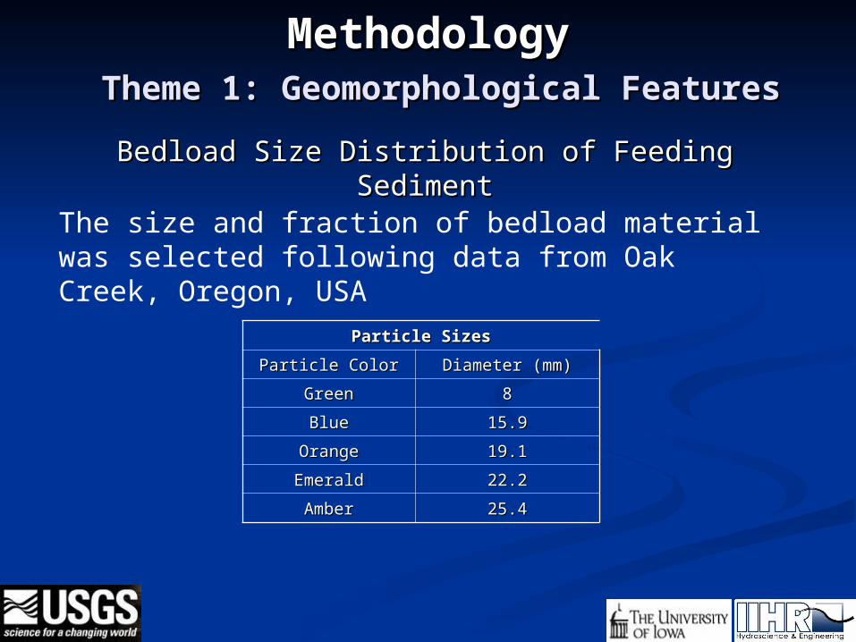
The size and fraction of bedload material was selected following data from Oak Creek, Oregon, USA
Particle SizesParticle Sizes
Particle ColorParticle Color Diameter (mm)Diameter (mm)
GreenGreen 88
BlueBlue 15.915.9
OrangeOrange 19.119.1
EmeraldEmerald 22.222.2
AmberAmber 25.425.4

Methodology Theme 1: Geomorphological
FeaturesClast Size
The clast size is defined as,The clast size is defined as,
ddclastsclasts ≈≈ 3d 3darmorarmor, where d, where darmorarmor = d = d5050 = 1.9 cm = 1.9 cm
thus, dthus, dclasts clasts = 5.5 cm= 5.5 cm
due to the size of the median particle matching the size due to the size of the median particle matching the size of the armored bed (Reid et al., 1992). of the armored bed (Reid et al., 1992).

Methodology Theme 1: Geomorphological
FeaturesSpacing of clasts
de Jong (1995) Papanicolaou and Kramer (submitted)

Methodology Theme 1: Geomorphological
FeaturesIncipient Conditions
To identify the incipient conditions for individual particles, the To identify the incipient conditions for individual particles, the concept of the probability of entrainment, Pconcept of the probability of entrainment, PEE, was employed , was employed
rather than the Shields diagram where:rather than the Shields diagram where:
T
EE
N
NP
T
EE
N
NP
T
EE
N
NP
T
E
EN
NP

Methodology Theme 1: Geomorphological
FeaturesIncipient Conditions
T
EE
N
NP
T
EE
N
NP
T
EE
N
NP
T
E
EN
NP
t = 0 min t = 1.5 min

Methodology Theme 1: Geomorphological
FeaturesBedload Feeding rate
Once a critical probability of entrainment is set (PE=0.02), a correspondence between PE and the dimensionless shear stress, cr
* (the Shields parameter) was developed where:
501
2**
gdSG
u
A dimensionless bedload, qA dimensionless bedload, qbb**, formula based on , formula based on * from * from
Paintal (1971) and calibrated by Strom et al. (2004) for Paintal (1971) and calibrated by Strom et al. (2004) for spherical particles was employed where:spherical particles was employed where:

Methodology Theme 1: Geomorphological
FeaturesBedload Feeding rateBedload Feeding rate
From dimensional analysis the bedload feeding rate [kg/m/s], qFrom dimensional analysis the bedload feeding rate [kg/m/s], qbb, ,
can be determined from can be determined from
This feeding rate was provided via feeding, well upstream of the clast section, so that the exiting bedload size distribution and transport rate was independent of initial conditions (Parker and Wilcock, 1993)

Experimental Setup
Head Tank
FLUME TILTED AT 15%
LEVEL FLUME
LiftingPoint
LiftingPoint
TailgateWeir
TailgateWeir
2'-6" 3'-0" 3'-0"3'-3"18x50Wide Flange Beam
W10x49Wide Flange
Beam
LipExtension
LipExtension
Brace
3'-0" 12'-0" 39'-0"
15'-0"
3'-0" 3'-0" 9'-0" 12'-0" 12'-0" 12'-0" 3'-0" 3'-0" 3'-0" 3'-0" 6'-3 7/8"
69'-3 7/8"
3'-0"3'-7 1/2"
LiftingMechanism
Flow
Head Tank
1'-3 3/4"
1'-9 3/4"
3'-0"
2'-6"
Head Tank
PLAN VIEW OF FLUME
TelescopingPipe
5'-11"
5'-6 9/16"
8.53°
8'-4 9/16"
6'-1 15/16"
14'-6 1/2"
5'-6"
2'-7"
Flume

Experimental SetupClast Section

Experimental Setup
-3Dy -2Dy -1Dy 0Dy
8Dx
7Dx
6Dx
5Dx
0Dx
1Dx
2Dx
3Dx
4Dx
9Dx
10Dx
• Acoustic Doppler Velocimeter (10 MHz ADV)
• 40 Measuring Locations with 15 point measurements per profile (Total of 600 point measurements )
• 3000 measurements per point, for obtaining velocity measurements of statistical significance (e.g., Nikora and Goring 1998, Papanicolaou and Hilldale 2002).
Flow Measuring Devices
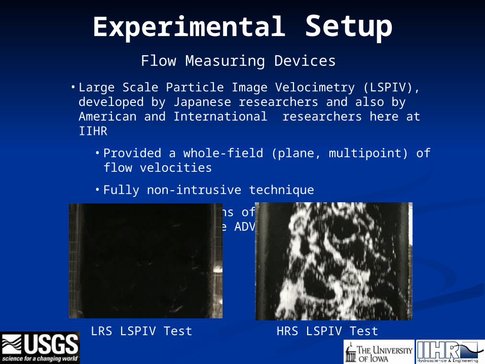
Experimental SetupFlow Measuring Devices
• Large Scale Particle Image Velocimetry (LSPIV), developed by Japanese researchers and also by American and International researchers here at IIHR
• Provided a whole-field (plane, multipoint) of flow velocities
• Fully non-intrusive technique
• Much quicker means of data collection in comparison to the ADV
LRS LSPIV Test HRS LSPIV Test

Experimental conditions(1)
Test Name(2)
(3)H
(cm)
(4)H/dclast
(m/m)
(5)Q
(m3/s)
(6)S (m/m)
(7)Ubulk
(m/s)
(8)Fr
(-)
(9)Re
(-)
(10)u*
(m/s)
A1a 0.017 4.4 0.8 0.02 0.0159 0.49 0.75 8.671E+04 0.08
A1b 0.017 4.4 0.8 0.02 0.0159 0.49 0.75 8.671E+04 0.08
A2a 0.021 4.4 0.8 0.02 0.0186 0.54 0.81 9.414E+04 0.09
A2b 0.021 4.4 0.8 0.02 0.0186 0.53 0.80 9.290E+04 0.09
A3a 0.026 4.4 0.8 0.03 0.0212 0.70 1.06 1.226E+05 0.10
A3b 0.026 4.4 0.8 0.03 0.0212 0.71 1.08 1.251E+05 0.10
A4a 0.030 4.4 0.8 0.03 0.0239 0.75 1.14 1.313E+05 0.10
A4b 0.030 4.4 0.8 0.03 0.0239 0.74 1.13 1.301E+05 0.10
B1a 0.017 19.25 3.5 0.13 0.0024 0.76 0.56 5.871E+05 0.07
B1b 0.017 19.25 3.5 0.13 0.0024 0.76 0.56 5.871E+05 0.07
B2a 0.021 19.25 3.5 0.14 0.003 0.78 0.57 6.020E+05 0.08
B2b 0.021 19.25 3.5 0.14 0.003 0.78 0.57 6.008E+05 0.08
B3a 0.026 19.25 3.5 0.14 0.0036 0.82 0.60 6.293E+05 0.08
B3b 0.026 19.25 3.5 0.14 0.0036 0.80 0.59 6.194E+05 0.08
B4a 0.030 19.25 3.5 0.15 0.0042 0.84 0.61 6.429E+05 0.09
B4b 0.030 19.25 3.5 0.15 0.0042 0.83 0.61 6.417E+05 0.09

Results
Bedload AnalysisQualitative Observations
for H/dclast = 3.5

Results
Test B1b
Test B2a
Test B3b
Test B4a

ResultsBedload Analysis
Qualitative Observations for H/dclast = 3.5
• Majority of clusters are deposited on the wake region of the clasts
• Some few …particles are deposited randomly throughout the test section if not located in the vicinity of a clast

Results
0.00
0.01
0.02
0.03
0.04
0.05
0.06
0.07
0.08
0.09
0.10
0 20 40 60 80
Time (min)
Bed
load
Rat
e (g
/m/s
)
Exiting Bedload Incoming Bedload
0.00
0.02
0.04
0.06
0.08
0.10
0.12
0.14
0.16
0 20 40 60 80
Time (min)
Bed
load
Rat
e (g
/m/s
)
Exiting Bedload Incoming Bedload
0.00
0.05
0.10
0.15
0.20
0.25
0.30
0 20 40 60 80
Time(min)
Be
dlo
ad
Ra
te (
g/m
/s)
Exiting Bedload Incoming Bedload
0.00
0.05
0.10
0.15
0.20
0.25
0.30
0.35
0.40
0.45
0 20 40 60 80
Time(min)
Bed
load
Rat
e (g
/m/s
)
Exiting Bedload Incoming Bedload
Test B1b Test B2a
Test B3b Test B4a

Results
0.120.48 0.70
0.951.24
Incoming Bedload
Exiting Bedload
DepositedBedload0
0.05
0.1
0.15
0.2
0.25
0.3
0.35
0.4
0.45
No
rmal
ized
Fre
qu
ency
Mass (g)
0.12 0.48 0.700.95
1.24
Incoming Bedload
Exiting Bedload
Deposited Bedload0
0.05
0.1
0.15
0.2
0.25
0.3
0.35
0.4
0.45
0.5
No
rmal
ized
Fre
qu
ency
Mass (g)
0.12 0.48 0.70 0.95 1.24
Incoming Bedload
Exiting Bedload
Deposited Bedload0
0.05
0.1
0.15
0.2
0.25
0.3
0.35
0.4
0.45
No
rmal
ized
Fre
qu
ency
Mass (g)
0.12 0.48 0.70 0.95 1.24
Incoming Bedload
Exiting Bedload
Deposited Bedload0
0.05
0.1
0.15
0.2
0.25
0.3
0.35
0.4
0.45
No
rmal
ized
Fre
qu
ency
Mass (g)
Test B1b Test B2a
Test B3b Test B4a

ResultsTest B1b
Stoss Wake
Green 0.0% 0.0%
Blue 1.5% 13.8%
Orange 0.0% 27.7%
Emerald 13.8% 29.2%
Amber 4.6% 9.2%
Test B4a
Stoss Wake
Green 0.0% 3.7%
Blue 0.0% 23.4%
Orange 0.0% 30.8%
Emerald 9.3% 24.3%
Amber 0.0% 8.4%
Test B3b
Stoss Wake
Green 0.0% 0.0%
Blue 0.0% 25.0%
Orange 0.0% 19.0%
Emerald 9.0% 37.0%
Amber 0.0% 10.0%
Test B2a
Stoss Wake
Green 0.0% 0.0%
Blue 0.0% 16.5%
Orange 0.0% 25.9%
Emerald 7.1% 32.9%
Amber 5.9% 11.8%

Results
Bedload AnalysisQualitative Observations
for H/dclast = 0.8
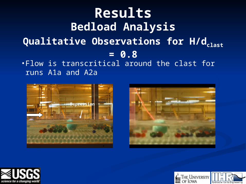
ResultsBedload Analysis
Qualitative Observations for H/dclast = 0.8
• Flow is transcritical around the clast for runs A1a and A2a
Depression

Results
• Supercritical flow with the presence of surface waves become pronounced for runs A3b and A4a
Bedload AnalysisQualitative Observations for H/dclast =
0.8
Surface Wave

ResultsBedload Analysis
Qualitative Observations for H/dclast = 0.8• Two different types of bed topography were observed for the low relative
submergence runs:
1. In-line clusters
2. Cluster–deposits
• In-line clusters (i.e. “streaks”) form during the transcritical flow runs, A1a and A2a
• In-line clusters spacing is dictated by clast spacing
• Cluster–deposits (known in the literature as dump-deposits, Billi, 1988) are generated during runs A3b and A4a
• Cluster-deposits spacing is dictated by surface waves

Results
Figure 18. Test A2a
Figure 19. Test A3b
Figure 20. Test A4b
Figure 17. Test A1a

Results
Bedload AnalysisQuantitative Observations
for H/dclast = 0.8

ResultsBedload Analysis
Quantitative Observations for H/dclast = 0.8
• For the low relative submergence, clusters exhibit a similar effect on bedload to clusters in the high relative submergence runs
• The only notable difference between the LRS and the HRS is that the depositional patterns are larger and distinguishable
• Incoming and exiting bedload are in phase with one another
• The larger percentage of particles are deposited in the stoss region with the most populated fractions being the emerald and amber

Results
0.00
0.01
0.02
0.03
0.04
0.05
0.06
0.07
0 20 40 60 80
Time (min)
Bed
load
Rat
e (g
/m/s
)
Exiting Bedload Incoming Bedload
0.00
0.02
0.04
0.06
0.08
0.10
0.12
0.14
0.16
0.18
0.20
0 20 40 60 80
Time (min)
Bed
load
Rat
e (g
/m/s
)
Exiting Bedload Incoming Bedload
0.00
0.10
0.20
0.30
0.40
0.50
0.60
0 10 20 30 40 50 60
Time (min)
Bed
lao
d R
ate
(g/m
/s)
Exiting Bedload Incoming Bedload
A1a A2a
A3b A4b
0.00
2.00
4.00
6.00
8.00
10.00
12.00
0.00 20.00 40.00 60.00 80.00
Lag Time (min)
Bed
load
Rat
e g
/m/s
Exiting Bedload Incoming Bedload

Results
0.12 0.480.70 0.95
1.24
Incoming Bedload
Exiting BedloadDeposited Bedload
0
0.05
0.1
0.15
0.2
0.25
0.3
0.35
0.4
0.45
No
rma
lize
d F
req
ue
nc
y
Mass (g)0.12 0.48 0.70
0.95 1.24
Incoming Bedload
Exiting Bedload
Deposited Bedload0
0.05
0.1
0.15
0.2
0.25
0.3
0.35
0.4
0.45
0.5
No
rmal
ized
Fre
qu
ency
Mass (g)
0.12 0.48 0.700.95
1.24
Incoming Bedload
Exiting Bedload
Deposited Bedload0
0.05
0.1
0.15
0.2
0.25
0.3
0.35
0.4
0.45
No
rma
liz
ed
Fre
qu
en
cy
Mass (g)
0.12 0.48 0.700.95
1.24
Incoming Bedload
Exiting Bedload
Deposited Bedload0
0.05
0.1
0.15
0.2
0.25
0.3
0.35
0.4
0.45
No
rma
liz
ed
Fre
qu
en
cy
Mass (g)
A1a A2a
A3b A4b

ResultsTest A1a
Stoss Wake
Green 0.0% 0.0%
Blue 0.0% 0.0%
Orange 36.4% 0.0%
Emerald 36.4% 0.0%
Amber 27.3% 0.0%
Test A2a
Stoss Wake
Green 0.0% 0.0%
Blue 8.5% 0.0%
Orange 29.2% 0.0%
Emerald 46.2% 0.0%
Amber 16.2% 0.0%
Test A4b
Stoss Wake
Green 0.0% 0.0%
Blue 4.2% 0.0%
Orange 16.7% 0.0%
Emerald 45.8% 0.0%
Amber 33.3% 0.0%
Test A1a
Stoss Wake
Green 0.0% 0.0%
Blue 7.7% 0.0%
Orange 13.5% 0.0%
Emerald 44.2% 0.0%
Amber 34.6% 0.0%

Flow AnalysisFlow AnalysisQuantitative Observations for H/dclast =
3.5 and *= 2.5 *cr
Quantitative Observations for H/dclast = 0.8 and *= 2.5 *cr

ResultsFlow Analysis
Quantitative Observations for H/dclast = 3.5 and *= 2.5 *cr• Analysis of the mean flow measurements performed during a run for
*=2.5*cr on the specified grid shown below aimed to provide an improved understanding of the flow structures around the clasts with the intent to complement the sediment observations of run B2a (H/dclast = 3.5 and *= 2.5 *cr)
-3Dy -2Dy -1Dy 0Dy
8Dx
7Dx
6Dx
5Dx
0Dx
1Dx
2Dx
3Dx
4Dx
9Dx
10Dx

0
5
10
15
20
Dep
th (
cm)
0
5
10
15
20
Dep
th (
cm)
0
5
10
15
20
Dep
th (
cm)
Transect 0Dy
0 50 100
Velocity (cm/s)
0
5
10
15
20
Dep
th (
cm)

ResultsFlow Analysis
Quantitative Observations for H/dclast = 3.5 and *= 2.5 *cr
0
2
4
6
8
10
12
14
0.1 1 10
(z+zo)/ks
u/u
*
log law
0D
1D
2D
3D
4D
5D
6D
7D
8D
9D
10D
Log Law Transect -3Dy
Log Law Transect -1Dy
0
2
4
6
8
10
12
14
0.1 1 10(z+zo)/ks
u/u
*
log law
0D
1D
2D
3D
4D
5D
6D
7D
8D
9D
10D

ResultsFlow Analysis
Quantitative Observations for H/dclast = 3.5 and *= 2.5 *cr
Transect 0Dy (Side View) Transect -1Dy (Side View)
Transect -2Dy (Side View) Transect -3Dy (Side View)

ResultsFlow Analysis
Quantitative Observations for H/dclast = 3.5 and *= 2.5 *cr
Plan View of the Streamwise Velocity at z = 0.6 cm Plan View of the Streamwise Velocity at z = 3.85 cm
Plan View of the Streamwise Velocity at z = 17.6 cm

ResultsFlow Analysis
Comparison of ADV and LSPIV
LSPIV Streamwise Velocity for
H/dclast = 3.5 and *= 2.5 *cr
Plan View of the Streamwise Velocity at z = 17.6 cm

ResultsFlow Analysis
Quantitative Observations for H/dclast = 0.8 and *= 2.5 *cr
• For the low relative submergence experiments, LSPIV measurements were utilized due to ADV measurements not being feasible at low flow depths
• The effects of roughness to the flow are well depicted at the free surface
• To link flow characteristics around clasts with cluster depositional patterns, the plan view LSPIV images were superimposed with plan view images of depositional patterns

ResultsFlow Analysis
Quantitative Observations for H/dclast = 0.8 and *= 2.5 *cr
LSPIV Streamwise Velocity for
H/dclast = 0.8 and *= 2.5 *cr

ResultsFlow Analysis
Superimposition Observation for H/dclast = 0.8 and *= 2.5 *cr
LSPIV Particles Overlayed with Bedload for H/dclast = 0.8 and *= 2.5 *cr

ConclusionsConclusions• This research examined the effects of relative submergence on cluster
formation.
• In the laboratory flume, spherical clasts were placed in a fixed grid atop a well-packed glass bead bed.
• Two relative submergences were investigated, namely the high and low relative submergences
• In the high relative submergence, sediment motion is governed by the particle Reynolds number.
• In the low relative submergence, the importance of the Reynolds number on sediment motion diminishes, and the Froude number becomes the governing parameter.

ConclusionsConclusions• The results of this study focused on:
1. The qualitative evaluation of the bed microtopography for the high and low relative submergence
2. A quantitative description of the bedload transport rates and their statistical properties
3. A detailed analysis of the flow characteristics around a clast
4. The coupling of flow with bed microtopography observations around a clast

ConclusionsConclusionsThe following specific conclusions can be drawn from this investigation:
1. Clasts placed at specified distances regulated the depositional dynamics atop the flume bed, thus minimizing the random formation of microstructures
2. For the high and low relative submergence experiments clasts/clusters worked as a sink for the incoming sediment
3. Cluster formation occurred randomly in space for the high relative submergence, while for the low relative submergence clasts appeared to control the areas where cluster formation occurred
4. For the high relative submergence, a larger percentage of incoming particles were deposited in the wake region. For the low relative submergence and for stress less than * = 2.5*cr, particles were mainly deposited in the stoss region of the clasts.

ConclusionsConclusions
5. For the high relative submergence, the plots of the velocity profiles indicated that the effects of the clasts were not felt significantly at the free surface of the flow where the log law in the outer layer appeared to adequately describe the measured observations.
6. For the high relative submergence, the effects of clasts on the flow were present within the zone of influence of clasts, which was typically found to be at 0.3-0.5 times the clast diameter in the vertical direction and 2 to 4 times the clast diameter in the streamwise direction

ConclusionsConclusions7. For the high relative submergence tests, several factors contributed to
the generation of secondary currents of Prandtl’s second kind, including
• The low aspect ratio (B/H < 5)
• The presence of the fixed grid of clasts,
• The feedback process between flow and clasts
8. The ADV measurements provided improved insight about the governing flow mechanisms for the high relative submergence runs. These mechanisms were described with
• flow upwelling at the center of the flume
• downwelling occurring along the flume walls

ConclusionsConclusionsThe following specific conclusions can be drawn from this investigation:
9. For the low relative submergence experimental runs, the near-bed flow structures (HS vortices, “Froudian” wakes, and hydraulic jumps) controlled the depositional patterns of the incoming sediment.