an unobserved components approach to separating land from ... · materialofeachstructure....
TRANSCRIPT

An Unobserved Components Approach to Separating Land
from Structure in Property Prices: A Case Study for the
City of Brisbane
Alicia N. Rambaldi(1), Ryan R. J. McAllister(2), Kerry Collins(2), Cameron S. Fletcher(3)
version: 23 June, 2011
(1)School of Economics, The University of Queensland, St Lucia, QLD 4072. Australia.
(2) Commonwealth Scientific and Industrial Research Organisation (CSIRO) Ecosystem Sciences, Boggo Road,
Dutton Park, Brisbane, QLD 4102. Australia
(3) Commonwealth Scientific and Industrial Research Organisation (CSIRO) Ecosystem Sciences, PO Box 780,
Atherton, QLD 4883. Australia
Abstract
The study develops a spatio-temporal model of hedonic pricing that explicitly separates
the land and the structure components of property prices. This is illustrated with a dataset
for Brisbane, Australia, constructed by combining commercial real estate, local government
databases and GIS-based spatial analyzes. The land component of prices has increased from
42% in 2000 to 66% in 2010. This has implications for a broad range of planning and policy
issues, including property tax rates, town planning, and options for climate adaptations.
Keywords: urban land prices, housing prices, state-space, unobserved components.
JEL: C5, C8, R1
1

1 Introduction
A property is a bundled good composed of an appreciating asset, land, and a depreciating asset,
structure. The importance of this distinction is increasingly recognised in the real estate literature
(see Bostic et al (2007)) as well as in the price index construction literature (see Statistics Nether-
lands and EuroStat (2011), Chapter 13 and Diewert et al (2010)). Bostic et al (2007) provides
an excellent exposition of the arguments. In particular, they argue that due to the mobility of
materials and labor, construction costs are generally uniform within a housing market and thus
it must be the case that asymmetric appreciation across properties within a market arise from
asymmetric exposure to common shocks to land values.
At any point in time the value of the structure is its replacement cost less any accumulated
depreciation. Thus, sufficiently large depreciation can result in the structure (improvements on
the land) declining in value over time (see (Malpezzi et al , 1987) and (Knight and Sirmans ,
1996) for an excellent discussion and treatment of modelling and accounting for depreciation and
maintenance of the structure).
This study proposes the use of a hedonic based unobserved components approach. Specifically, land
and structure are viewed as two additive components of the price. The underlying trend in each
component is determined by hedonic characteristics intrinsic to that component. For instance, the
size and age of the dwelling are unique characteristics of the structure, while the size of the parcel
and distance to amenities are unique characteristics of the land. In particular, previous studies
have identified the importance of the structure’s age and size, and lot size heterogeneity (Knight
and Sirmans (1996) and Diewert et al (2010)). The data used for this study are from the city
of Brisbane, Australia, where there are two commercial providers of real estate transactions that
cover most of the urbanized areas in the country. Unfortunately, the age of the structure (building
age) and the size of the structure are not available through the datasets from these commercial
providers. Thus, government databases with supplementary GIS-based spatial analyzes were used
to assemble a unique set of hedonic attributes for an Australian dataset.
The method of estimation and imputation of the structure and land components of property values
2

used in this study is different from those in previous studies. An unobserved components approach
is used to estimate a time-varying hedonic model with attributes that capture: 1) structure, such
as the number of bedrooms, structure size and age; and 2) land, including lot size, location with
respect to landmarks, and location-related characteristics (e.g. frequency of flooding). There is
no common trend in the model as it would capture the combined trends in land and structure.
This problem was identified in studies using conventional hedonic models with an intercept term
(Diewert et al (2010)). The method proposed allows identification of the land and structure com-
ponents of property prices through the memory built into the time-varying parameters associated
with specific hedonic characteristics of each component.
The paper is organised as follows: Section 2 presents the unobserved components model proposed
for the decomposition. This includes a spatially correlated error to account for omitted hedonic
characteristics that might create dependence in the random error component. Section 3 describes
that data used to illustrate the method. The dataset was assambled from a number of sources
and this is discussed in some detail. Section 4 presents the results and compares them to those
produced by the State Valuation Service of the Queensland’s government. Section 5 concludes.
2 Model
Similar to previous studies (Bostic et al (2007) and Diewert et al (2010)) three orthogonal
components are defined, land (L), structure (H) and noise. In this study these components are
defined within a time-varying parameter framework with spatial errors.
yt = XLt β
Lt +XH
t βHt + εt
εt = ρWtεt + ut (1)
βct = βct−1 + ηct
where,
3

yt vector sale price properties sold in t
Xct matrix hedonic characteristics associated with c = L,H for properties sold in t
βct vector hedonic coefficients associated with component c = L,H
ρ spatial correlation parameter
εt spatially correlated error
ut ∼ N(0, σ2uI)
ηct ∼ N(0, σ2ηI)
Wt a row stochastic spatial weights matrix, Wt =
wii,t = 0
wij,t 6= 0 if neighbouring
The model has no common intercept trend to avoid capturing combined trends of land and struc-
ture. In this paper the nearest neighbours are computed using a Delaunay triangulation. A
detailed exposition of Delaunay triangulations can be found in LeSage and Pace (2009) Section
4.11. When W is derived using Delaunay triangles, it represents the nearest m neighbours, W 2
represents neighbours to neighbours, and so on.
The model (1) is cast in a state-space form,
yt = Ztαt + εt
αt = αt−1 + ηt
where,
εt ∼ (0, Ht)
ηt ∼ (0, Qt)
α0 ∼ (0, P0)
Zt =
[XLt XH
t
], a Nt×K matrix, Nt is the number of properties sold in t; K is the number of
hedonic characteristics (land plus structure).
4

αt =
βLt
βHt
Ht = σ2
u (INt − ρWt)−1 (INt − ρWt)
−1′
Qt = σ2ηIK
The parameters αt are estimated by a Kalman filter (KF) and smoother (S) given estimates of the
hyperparameters, ψ =[σ2u, σ
2η, ρ], which are estimated by maximum likelihood. The KF algorithm
provides a value of the likelihood function to find the estimates of ψ in a standard state-space
framework (see Harvey (1989) or Durbin and Koopman (2001)).
Given estimates of αt, predictions of the sale price of the property, land and structure components
are,
yt|T = Ztαt|T (2)
where,
αt|T is the S estimate of βt =
βLt
βHt
yLt|T = XL
t βLt|T (3)
where,
βLt|T is the subset of αt|T corresponding to hedonic characteristics of land
yHt|T = XHt β
Ht|T (4)
βHt|T is the subset of αt|T corresponding to hedonic characteristics of structure
5

3 Data
A purposely built dataset was assembled for this project. Real estate property sales data purchased
from a commercial provider (RP Data Ltd) were merged with a number of other datasets. The
real estate sales dataset included information of the sale date, sale price, the type of sale, land
area, street address, the land parcels’ unique identifier (Lot/Plan number), geographical location,
and land use, as well as specific house structure variables including the number of bedrooms,
bathrooms, and car spaces.
For this study only normal property sales (all other sales, such as gifted or partial sales were
excluded) with a land use description of vacant land (i.e. Vacant – large house site and Vacant –
urban land) or dwelling (i.e. Dwelling – large house site or Single Unit Dwelling) were used.
Due to the incomplete nature of the commercially provided data substantially cleaning was re-
quired to remove obvious errors and build a more complete dataset. This process involved cross
checking against additional data sources including local government sources (e.g. the council’s
property planning and development website – PD Online), other real estate data sources (e.g.
www.homepriceguide.com.au and www.realestate.com) and aerial imagery sources. Online
sources such as Google Earth (using its Historical Imagery feature) and Google Street View. Once
cleaned the dataset was combined with numerous other information sources, such as geospatial
data, aerial imagery, and historical council records, to build a more comprehensive set of hedonic
characteristics.
The age of the structure (i.e. the year it was built) is a key variable but one often not available in
Australian datasets. Only around 7% of the commercially purchase dataset were supplied with a
build year. To establish a proxy for build year/age of the structure online sources, largely Google
Street View, were used to view each property and determine, through expert knowledge, a build
era (The University of Queensland; Apperly et al. 1994; Wikipedia 2010; Wilcox 2009). The
identified eras were pre-war (pre-1946), post-war (1946-1960), late twentieth century (1960-2000)
and contemporary (2000 onwards). At the same time, this process was also used to collect the
additional hedonic characteristics of number of levels of each structure and the building and roof
6

material of each structure.
Geospatial data were used in the determination of the distance of properties to key features (e.g.
parks, train stations, schools, and waterways), their minimum and maximum ground levels, and
the footprint of houses in one of the case study areas. All spatial calculations were done using
the ESRI ArcGIS platform. Distances to features of interest were calculated using the Euclidean
distance tool. This was a measurement of the straight-line distance from the centroid of each
land parcel to the closest object of interest, such as a park, train station, bus stop, school, the
coastline or a waterway. The calculated distance values were exported to the point layer using
the Extract Values to Points tool. The minimum and maximum ground levels of each land parcel
were determined from a digital elevation model (DEM) at a spatial resolution of 5 m created
from LiDAR data (DERM). The Zonal Statistics tool within the Spatial Analyst toolbox was
used to summarise the values of the DEM within the boundaries of each land parcel, determining
the minimum and maximum ground heights of each unique land parcel. Building footprints were
determined using a grid based modelling approach on LiDAR data to a 10m2 level of accuracy.
The dataset contains 3944 residential sales records1 Figure 1 shows the distribution of sales for
each year in the sample, 1970 to 2010Q1.
Figure 1 here
The hedonic characteristics used in the modelling are presented in Tables 1 and 2. The dataset is
from a single suburb and there is some unavoidable homogeneity, e.g. the majority of the structures
are either pre-war or post-war (1946 marks a change in local architecture). This suburb, which
we do not identify due to confidentiality agreements, is ≈ 5 kms from Brisbane’s Central Business
District and is an older, well established suburb. There is a small proportion of sales of vacant
land concentrated in the later part of the sample, which appear to play a crucial role in the ability
to separate the land from structure.
Tables 1 and 2 here1The data contain ∼ 1610 properties, with an average of ∼ 3 sales records each.
7

4 Results
The modeling is designed to provide predictions of two additive components (land and structure)
and not intended to provide estimates of the marginal effects (shadow prices) of hedonic charac-
teristics (Figure 2). Due to the small number of observations in the sample, the time period for
estimation, t, in model (1) is a year. Ideally the model should be run at a monthly or quarterly
level of disaggregation. In spite of the short time period available, the model performs well. The
squared correlation between actual and predicted sale price, R2, over the sample is 0.81. The
decomposition of the price seems meaningful only after vacant land sales are observed (1988 on-
wards). Before 1988 the decomposition yields negative values for the land component, similar to
findings by Diewert et al (2010). This indicates sales of vacant land might be crucial to iden-
tifying the two components. There is a very small number of sales of vacant land in the sample
(87 properties); however, they greatly improve the ability of the model to decompose prices. The
time-varying parameter model seems to make efficient use of the vacant land sales.
Figure 2 here
The proportion of sale price due to land vale has increased from ≈ 42% to ≈ 66% between 2000
and 2010 (Figure 3). Existing estimates for Brisbane (ABS Housing Price Index), showed large
increases in residential properties prices in Brisbane between 2000 and 2008, with the majority of
that increase occurring in the period 2000 to 2005. The general view of government and the market
is that this is primarily due to land price increases in response to regional population growth.
Figure 3 here
The sample used in this study is small and for properties located within a particular suburb very
close to the Brisbane CBD. As such the empirical results are an illustration of the method and
cannot be used to make inferences to other areas of Brisbane or other types of property products
such as units, townhouses or commercial property. However, the results can be compared to the
8

valuations of the individual properties in the sample to those made by the Department of Envi-
ronment and Resource Management (DERM)- State Valuation Service. DERM is a department
of the state of Queensland with duties of land valuation under the Land Valuation Act.
The recently released report from the Valuer-General of the state of Queensland (State Valuation
Service (2011)) indicates the method of valuation for urban land has changed from 2011 to a
method known as ’site valuation.’ The method used to valuate urban land during the sample
period of this study is known as ’unimproved value.’ The new method is the same used across
other states in Australia and argued as more reflective of the market value of land. The method
proposed in this paper is a market model based valuation method in that the observed sale price
of a property is used to fit a willingness to pay model. The model is a hedonic based model which
predicts the trend in land and structure values given the hedonic characteristics of the properties.
Land valuations for the years 2009 and 2010 are available through the DERM website. The median
of the ratio of the DERM land valuation to the observed sale price of the property are compared to
the median of the ratio of the model’s land valuation to the sale price of the property. These results
are presented in Table 3. As stated, due to the small sample, the unit time period of estimation
of the model is annual; however, the predictions for properties sold within a given month are
aggregated for the presentation.
Table 3 here
The report from the Valuer-General indicates that “Brisbane was last revalued in 2010, and resi-
dential value movements have generally been mixed.” (State Valuation Service (2011), page 6).
This is consistent with the estimates from the model which show the median proprtion due to the
land component for 2010 to be much higher than that in 2009. The proportion of the land value
as a ratio of the predicted price (Figure 3) is close to 0.7, while the proportion of the predicted
land value to the observed sale price is 0.78 for 2010. The equivalent predictions for 2009 are 0.72
and 0.57, respectively. The model produces significant lower land valuations for 2009. This could
be a combination of the slower market in 2009 and a composition of sales effect (that is the sample
of houses that were sold in 2009).
9

5 Conclusions
The movement of property prices is a crucial indicator of economic performance. They are used
as indicators of potential price bubbles and in deliberations to set official interest rates. Local
taxes in Australia are based on land valuations, and the perception that these valuations are
obtained through ad-hoc procedures has driven recent controversy. The relative contribution of
land and structure to aggregate price has important implications for planning, policy and the
debate on housing affordability. Given this importance, the value of hedonic based price imputation
is substantial as this is a model based approach and thus it can be replicated.
A practical application of this understanding of the relative contribution of land and structure
to property value is in planning adaptation to future climates. The Intergovernmental Panel
on Climate Change identified the Brisbane region as particularly vulnerable because its growing
population is clustered in low lying coastal areas exposed to storm surge and flooding. Economically
rational adaptation pathways need to be developed, and understanding how much of a property
represents an appreciating asset (i.e. land) versus a depreciating asset (i.e. structure), will critically
determine the logic of spending now to defend against future events. Our study shows that as land
value represents an increasingly larger proportion of property values in major urban areas, cost-
benefit assessments of adaptation pathways will need to think beyond benefits accrued due to
avoided damage to infrastructure and also consider avoided loss of land assets as a major store of
personal wealth.
10

References
Apperly, R., R. Irving, P. Reyonlds (1995) "A Pictorial Guide to Identifying Australian Architec-
ture”
Basu S. and T. Thibodeau (1998), "Analysis of Spatial Autocorrelation in House Prices," Journal
of Real Estate Finance and Economics, 17:1, pp 61-85.
Bostic, R.W., Longhofer, S. D., and C. L. Redfearn (2007), “Land Leverage: Decomposing Home
Price Dynamics.” Real Estate Economics, 35:2, pp. 183–208.
Clapp J.M, H.J. Kim and A. E. Gelfand (2002), “Predicting Spatial Patterns of House Prices Using
LPR and Bayesian Smoothing,” Real Estate Economics, 30:4, pp. 505-532.
Diewert, W. E., Jan de Haan and R. Hendriks (2010), “The Decomposition of a House Price index
into Land and Structures Components: A Hedonic Regression Approach,” Paper presented at
the General Conference of the International Association for Research in Income and Wealth
(IARIW), St. Gallen, Switzerland, 22-28 August 2010.http://www.iariw.org/papers/2010/
2aDiewert.pdf
Durbin, J. and S. J. Koopman (2001), Time Series Analysis by State Space Methods, Oxford
Statistical Science Series. Oxford University Press Inc.
Harvey, A. C (1989), Forecasting, Structural Time Series Models and the Kalman Filter, Cam-
bridge.
Knight, J.R. and C.F. Sirmans. 1996. Depreciation, Maintenance, and Housing Prices. Journal of
Housing Economics 5: 369–389.
LeSage, J. and Pace, K. (2009) Introduction to Spatial Econometrics, Boca Raton: Chapman &
Hall.
Malpezzi, S., L. Ozanne and T. Thibodeau. 1987. Microeconomic Estimates of Housing Deprecia-
tion. Land Economics 6: 372–385.
11

State Valuation Service, Department of Environment and Resource Management, State of Queens-
land (2011), “ Valuer-General’s Property Market Movement Report. Snapshot of the 2011 valu-
ation”
Statistics Netherlands and EuroStat (2011), Handbook on Residential Property Price In-
dices, v3.0 (draft version available for comments). Statistics Netherlands and EuroStat.
http://epp.eurostat.ec.europa.eu/portal/page/portal/hicp/documents/Tab/Tab/
RPPI_Handbook%20_combined_V3_0.pdf
Wilcox, L. (2009) Housing Styles, http://www.hotpropertyspecialists.com.au/articles/
housing-styles.html
12

0
40
80
120
160
200
240
280
70 75 80 85 90 95 00 05 10
5 . 0 5 . 0
8 . 07 . 0
11. 012. 0 12. 0
17. 0
21. 0
12. 0
30. 0
27. 0
24. 0
43. 044. 0
46. 0
38. 0
67. 0
105. 0
94. 0
128 . 0
106. 0
130. 0
140. 0
133. 0
107. 0
115. 0
137. 0
131 . 0
142 . 0
175. 0
226. 0
239 . 0
225 . 0
165. 0
197. 0
213 . 0
223 . 0
173 . 0
170. 0
41. 0
Figure 1: Number of Sales Observed Per Year
13

-200,000
0
200,000
400,000
600,000
800,000
1,000,000
70 75 80 85 90 95 00 05 10
Median Observed Price Sum Median Predicted ComponentsMedian Predicted Land Value Median Predicted Structure Value
Vacant Sales Observed
Figure 2: Observed Sale Price and Decomposition of Predicted Price into Land and StructureComponents (year median shown)
14

0.1
0.2
0.3
0.4
0.5
0.6
0.7
0.8
0.9
1.0
90 92 94 96 98 00 02 04 06 08 10
LAND_PROPORTIONSTRUCTURE_PROPORTION
Figure 3: Proportion of Price Due to Land and Structure
15
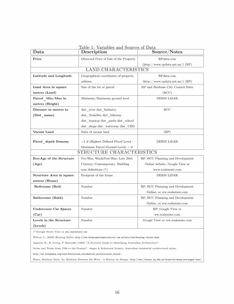
Table 1: Variables and Sources of DataData Description Source/NotesPrice Observed Price of Sale of the Property RPdata.com
(http://www.rpdata.net.au/) (RP)
LAND CHARACTERISTICSLatitude and Longitude Geographical coordinates of property
address
RPdata.com
(http://www.rpdata.net.au/) (RP)
Land Area in square
metres (Land)
Size of the lot or parcel RP and Brisbane City Council Data
(BCC)
Parcel_Min/Max in
metres (Height)
Minimum/Maximum ground level DERM LiDAR
Distance in metres to
(Dist_name)
dist_river dist_Industry
dist_TrainStn dist_bikeway
dist_busstop dist_parks dist_school
dist_shops dist_waterway dist_CBD
BCC
Vacant Land Sales of vacant land (RP)
Flood_depth Dummy =1 if (Highest Defined Flood Level -
Minimum Parcel Ground Level) > 0
DERM LiDAR
STRUCTURE CHARACTERISTICSEra-Age of the Structure
(Age)
Pre-War; War&Post-War; Late 20th
Century; Contemporary. Building
eras definitions (a)
RP, BCC Planning and Development
Online website, Google View or
www.realestate.com
Structure Area in square
metres (House)
Footprint of the house DERM LiDAR
Bedrooms (Bed) Number RP, BCC Planning and Development
Online, or ww.realestate.com
Bathrooms (Bath) Number RP, BCC Planning and Development
Online, or ww.realestate.com
Undercover Car Spaces
(Car)
Number RP, Google View or
ww.realestate.com
Levels in the Structure
(Levels)
Number Google View or ww.realestate.com
(a)Google Street View or www.realestate.com
Wilcox, L. (2009) Housing Styles, http://www.hotpropertyspecialists.com.au/articles/housing-styles.html
Apperly, R., R. Irving, P. Reyonlds (1995) "A Pictorial Guide to Identifying Australian Architecture”;
Styles and Terms from 1788 to the Present". Angus & Robertson Sydney; Australian residential architectural styles,
http://en.wikipedia.org/wiki/Australian_residential_architectural_styles ;
Home, Brisbane Style. In: Brisbane Between the Wars - A History by Design. http://www.library.uq.edu.au/fryer/brisbane_btw/page5.html;
16

Table 2: Descriptive StatisticsMin
Max MedianPrice $2,600
$4,710,000 $215,000
Land 1812218 607
House 44.961000 174.20
Vacant Land 087
Parcel_Min in metres (Height_Min) 0.08480.625 20.107
Distance in metres todist_river dist_Industry
dist_TrainStn dist_bikewaydist_busstop dist_parks dist_schooldist_shops dist_waterway dist_CBD
0.9520; 0; 0.0141;
0.0100; 0.0112; 0.0050;
0.0400; 0; 0.0050;
2.46114.7740; 2.6157; 3.1689;
1.5055; 0.5040; 0.5629;
1.2339; 1.0894; 1.6236;
5.7696
3.0447; 0.9101; 1.4041;
0.5597; 0.1812; 0.1589;
0.4451; 0.3312; 0.5256;
3.9667
AgePre-War
1942
War/Post-War1462
Late 20th Century (1980s and 1990s)290
Contemporary (2000s)168
Bedrooms 06 3
Bathrooms 03 1
Undercover Car Spaces 05 2
Levels in the Structure 02 1
17

Table 3: Ratio of Land Valuation to Observed Property Sale Price (median over number of prop-erties)
Month DERM(∗) MODEL # PropertiesJan-09 0.721 0.620 13Feb-09 0.704 0.708 11Mar-09 0.762 0.578 16Apr-09 0.741 0.563 17May-09 0.746 0.564 16Jun-09 0.675 0.555 9Jul-09 0.738 0.578 11Aug-09 0.673 0.582 13Sep-09 0.734 0.589 14Oct-09 0.617 0.487 19Nov-09 0.683 0.495 12Dec-09 0.716 0.543 15Jan-10 0.581 0.811 6Feb-10 0.636 0.828 22Mar-10 0.748 0.765 7Apr-10 0.862 0.946 3May-10 0.315 0.374 2Sep-10 0.703 0.907 1
Median 2009 0.716 0.564 166Median 2010 0.664 0.775 41(∗)Department of Environment and Resource Managementhttp://www.derm.qld.gov.au/property/index.html
18