Eleventh Floor, Menzies Building Monash University, Wellington Road CLAYTON Vic 3800 AUSTRALIA Telephone: from overseas: (03) 9905 2398, (03) 9905 5112 61 3 9905 2398 or 61 3 9905 5112 Fax: (03) 9905 2426 61 3 9905 2426 e-mail: impact@buseco.monash.edu.au Internet home page: http//www.monash.edu.au/policy/

Analysing a Hypothetical Pierce’s

Disease Outbreak in South Australia Using a Dynamic CGE Approach

by

GLYN WITTWER Centre of Policy Studies

Monash University

SIMON MCKIRDY The Cooperative Research Centre

for National Plant Biosecurity

RYAN WILSON Plant Health Australia

General Working Paper No. G-162 September 2006

ISSN 1 031 9034 ISBN 0 7326 1569 0

The Centre of Policy Studies (COPS) is a research centre at Monash University devoted to quantitative analysis of issues relevant to Australian economic policy.

1

Analysing a hypothetical Pierce’s disease

outbreak in South Australia using a dynamic

CGE approach

Glyn Wittwer1, Simon McKirdy2 and Ryan Wilson3

Abstract

A dynamic computable general equilibrium model provides a tool for analysing the regional

economic consequences of a hypothetical plant pest incursion. The model is very detailed at

the industry and regional level. It includes a theory of regional labour market adjustment. In

our example, a hypothetical Pierce’s disease incursion, direct regional economic losses are

magnified by consequent depressed investment in downstream wine processing sectors.

Following elimination of the disease, it takes a number of years for the region to recover fully.

Key words: plant disease, CGE modeling

JEL classification: C68, Q11, Q68.

1 Centre of Policy Studies 2 The Cooperative Research Centre for National Plant Biosecurity 3 Plant Health Australia

2

3

Contents

1. Introduction 1 1.1 A dynamic, general equilibrium, multi-regional approach 1 2. Background 5 3. The model 8 4. The scenario 12 5. Conclusion 18 References 19 Appendix: a no-recovery scenario 25

4

1

1. Introduction

The WTO Sanitary and Phytosanitary (SPS) Agreement does not allow a purely precautionary

approach to quarantine restrictions except as a temporary measure (WTO, 1994). This implies

that quarantine rules must accept a certain level of risk of pest transmission arising from

international trade. It is helpful for policy makers to have at their disposal an economic model

that estimates the economic impacts of a particular plant pest.4 This can assist in evaluating

expected welfare losses against the economic benefits of trade. It may also compare the

economic consequences of a successful campaign with those of a failed campaign or

inadequate response to an incursion.

The present study uses a dynamic computable general equilibrium (CGE) model to analyse the

regional and national economic impact of a hypothetical plant pest incursion. This approach

has been motivated by new cost sharing arrangements between the government and plant

industries in Australia to deal with a broad range of potential emergency plant pest incursions

(see www.planthealthaustralia.com.au). The dynamic model may quantify different policy

responses to an incursion, ranging from a do-nothing approach to ongoing attempts at

eradication and management.

1.1 A dynamic, general equilibrium, multi-regional approach

Previous studies have concentrated mainly on a partial equilibrium approach (see Mumford,

2002). There are a number of motivations for moving to a general equilibrium approach in

examining the costs of pest incursions. Policy makers may prefer to measure social costs and

benefits, rather than industry- or commodity-specific effects, given the involvement of public

funding in pest prevention and management. Partial equilibrium (PE) approaches provide a

method for such estimation, but leave out some of the economic effects that might be highly

relevant to the analysis, including reallocation of capital and labour between sectors and real

4 International Plant Protection Convention definition of a “pest” is used here, being “any species, strain or biotype of plant, animal or pathogenic agent injurious to plants or plant products” unless indicated otherwise.

2

wage impacts, and the impacts on related industries. In addition, PE approaches measure only

the direct impacts of a scenario. Indirect impacts include, for example, the impact of changing

industry costs on the general price level, changing industry incomes on investment and

regional aggregate consumption, and the associated impacts on other sectors. Consequently,

PE approaches tend to underestimate the overall impact by excluding indirect effects. On the

other hand, particularly in the case of smaller crops of a regional rather than national interest,

for which published statistics with an input-output level of detail are not available, the CGE

approach may in the past have been perceived as either impractical or cumbersome. The

database and theory of TERM (The Enormous Regional Model, Horridge et al., 2005), used in

the present study, overcomes such concerns, by allowing CGE modeling at a regional and

sectoral level not previously available. The cornerstone of TERM is a master database

distinguishing 167 sectors and 58 regions. In applications, it is computationally convenient to

aggregate the model to the focus of the study. This allows us to combine very detailed

industry-level data with the full theory of a CGE model. The data are discussed in more detail

in section 3.

While agriculture accounts for a relatively small share of GDP in Australia (around 3.5 per

cent, Australian Bureau of Statistics 2005a), regions away from the major cities tend to be

relatively dependent on primary activities. An incursion that disrupts agriculture in a particular

region may have little effect nationally. However, at the regional level, it may have severe

impacts on employment opportunities and household incomes. The regional labour market

theory of the model, as described in section 3.1, allows real wages, employment and, in the

long run, labour supply at the regional level to deviate from the baseline forecast. If labour

supply in one region decreases in the long run due to deterioration in local labour market

conditions (stemming from a negative impact such as a disease incursion), labour supply in

other unaffected regions will increase correspondingly, as we assume in the long run that

national labour supply and employment will return to baseline forecast levels. Events of

economic significance at the regional level are important to policy makers, not only because

politicians are elected by region. The four largest cities in Australia (i.e., Sydney, Melbourne,

Brisbane and Perth), which account for around 55 per cent of the national population, are also

3

growing at a faster percentage rate than the national population: events adverse to the

prosperity of non-urban regions exacerbate this trend.

An alternative to a CGE modeling approach is to use input-output analysis based on Barossa

Valley data. This approach is defensible in so far as the Barossa Valley is small compared

with the Australian economy, so that losses and gains in the region have a relatively small

national impact. However, it has limitations. Input-output models are linear, being able to

solve for prices alone or quantities alone, without doing both simultaneously. This would omit

price-induced substitution from our study, which is potentially important for the Barossa wine

sectors, which source some grapes from outside the region. This approach would also

potentially exaggerate national losses, as it would not account for diversions of labour and

investment to other regions. Moreover, the input-output approach uses comparative statics: we

believe a dynamic approach is most suitable for this study.

There are several advantages in choosing a dynamic model for this application. An incursion

may persist for several years, during which time crop yields may fall, plantations may be

removed and, due to additional spraying and precautionary measures, costs per hectare may

rise. Regional impacts and national welfare effects therefore have a time path. Another

advantage of the dynamic approach is that the magnitude of welfare losses will depend on

whether an industry is expanding or shrinking: an incursion that reduces output in a shrinking

sector will have smaller consequences than in the case of an expanding sector. Dynamics are

also helpful in the treatment of compensation for lost output or destroyed plantations: lump

sum payments may be treated as reduction in the stock of debt in a region (i.e., as a transfer

from one region to another), so that no out-of-model calculation is required to convert it to an

annualised flow.

Endogenous investment responses and their linkage to capital accumulation are a crucial part

of dynamic modelling. Yet, we do not endogenise investment in the winegrape sectors in our

application. This is because our scenario concerns hypothetical disease outbreaks that threaten

the local winegrape sectors. The response to the outbreak involves a combination of actions by

private grape growers and coordination of disease management and quarantine restrictions by

4

a statutory authority, Plant Health Australia. We model vineyard removal as an exogenous

reduction in capital stocks and vineyard land. During the recovery/replanting phase in the first

scenario, we ascribe exogenous shocks to the investment levels of the grape sectors.

The dynamic theory of investment does apply to other sectors. Notably, investment levels in

the downstream wine sectors will be affected. As the scarcity of winegrapes rises with the

disease outbreak, the price of grapes purchased by wineries will rise, raising the costs of

winery production and lowering rates of return on winery capital. Consequently, winery

investment levels will fall relative to a baseline in which there is no disease outbreak. In turn,

sectors whose sales are mainly in the local economy will be adversely affected by any regional

downturn, with consequent falls in investment. Dynamics are also important in the labour

market theory, elaborated in section 3.5.

The lag between plantings and commercial grape yields, which is typical of plantation crops,

requires special treatment in the model. We use delayed productivity shocks, assuming that

initial plantings lower the average productivity of vineyards as they are not yet bearing. That

is, an x% increase in vineyard area by new plantings initially lowers productivity (relative to

pre-outbreak productivity) by x% (excluding yield losses in vineyards that remain intact).

Commercial yields in a region such as the Barossa would commence three years after

planting, with full yields being realized after 5 years. However, some of the vineyards

removed following the disease outbreak would have been aged and of relatively high quality.

We cannot assume that within a decade or so, the quality of grapes in new vineyards will yet

be equal to that of the vineyards prior to the disease outbreak. Therefore, when full yields are

restored, we assumed that winegrape productivity in the Barossa Valley is still slightly less

than pre-disease levels.

A previous study by Wittwer et al. (2005) considered a hypothetical outbreak of Karnal bunt

in wheat in Western Australia in a dynamic, multiregional CGE model. The present study

differs in several ways. First, the major source of losses arising from Pierce's disease will be

real output rather than quarantine-imposed losses. Second, the level of regional disaggregation

is more detailed in this level. Instead of the region of interest being modelled at the state level

5

in a bottom-up form, with the sub-state or statistical division detail being presented in top-

down form, as in Wittwer et al. (2005), the statistical division of interest is modelled in

bottom-up form in the present application. That is, each statistical division of interest has its

own input-output database, behavioural equations and trade matrices with other regions and

the rest of the world. In particular, the regional labour market theory operates at the statistical

division rather than state level. Third, we are dealing with a pest affecting a perennial (vine

stocks) rather than annual plant (wheat). The implication is that destruction of the plant

potentially will reduce incomes for a number of years to come. In this sense, vineyards or

orchards are a form of capital, with initial investment over several years leading to eventual

returns for many years to follow. The welfare implications of capital destruction, in this case,

removal of vineyards, are more readily measured in a dynamic than comparative static

framework, as it accounts for both stocks and flows. As with the earlier study, the dynamic

approach allows us to update the model's database year-by-year. This is particularly relevant

for the grape and wine sectors, which have exhibited extraordinary growth in Australia since

the late 1990s (Anderson and Norman, 2003).

2. Background

2.1 Pierce's disease

Pierce's disease is a serious bacterial disease, caused by Xylella fastidiosa, that kills

grapevines. The bacterium can reside in the water conductive system (xylem) of plants and

eventually block water movement in the plant. Vines develop symptoms when the bacteria

block the water conducting system and reduce the flow of water to affected leaves. Water

stress begins in mid-summer and increases through autumn. Once infected, grapevines

become nonproductive and may die within one to two years after infection (Varela et al.

2001). Pierce's disease is currently restricted to North America through to Central America

and has also been reported from some parts of northwestern South America. The disease is

restricted to regions with mild winters. The disease is less prevalent where winter

temperatures are colder, such as at higher altitudes, farther inland from ocean influences, and

at more northern latitudes (see http://nature.berkeley.edu/xylella/index.html).

6

X. fastidiosa has a very large host range and many plant species may host the pathogen

without having any symptoms of disease (Luck et al. 2002). The bacterium is spread

(vectored) from plant to plant by xylem feeding insects. The most important insect vector is

the glassy winged sharpshooter (GWSS) (Homalodisca coagulata). The introduction of

GWSS into southern California has dramatically changed the distribution and importance of

Pierce's disease (Varela et al. 2001). There are several reasons why GWSS is a more

important vector. It has faster movement and greater dispersal in vineyards. It feeds much

lower on the cane than other sharpshooters resulting in infections that are more likely to

survive the winter. This then enables vine-to-vine spread of Pierce's disease, which does not

occur with other vectors. It feeds on dormant grapevines during the winter, and it will breed

in large numbers in citrus orchards that are often adjacent to vineyards (see

http://nature.berkeley.edu/xylella/index.html).

Australia is presently free from X. fastidiosa and H. coagulata. Both have been identified as

serious threats to Australia's viticulture industry and research has indicated that most of

Australia's viticultural regions are suitable for the establishment and spread of both the

pathogen and its vector (Luck et al. 2002; Hoddle 2002; Hoddle 2004). The likelihood of

entry of Pierce’s disease and GWSS in Australia has been assessed as “moderate” and the

subsequent likelihood of establishment as “high” (Luck et al. 2001) though this likelihood has

not been quantified. The likelihood of entry into Australia was assessed on the known

occurrence of attempted illegal importation of grapevine budwood, the wide range of other

hosts for the GWSS and the recent history of spread of the pathogen and vector. As such an

active quarantine program is in place in Australia to minimise the risk of entry of either X.

fastidiosa or H. coagulata. This includes quarantine treatments for imported table grapes to

minimise the likelihood of introduction through this pathway.

2.2 The contribution of vineyards and wine to the local economy The Barossa Valley accounts for approximately 0.2 per cent of national economic activity, so

that even a regionally devastating economic event may transmit to a small impact at the

national level. The valley is one of South Australia's oldest grape growing regions. The state's

vineyards were never decimated by phylloxera, which is under official control and contained

7

within a small region in Victoria, so that it retains some vineyards dating back to the 1840s,

with heritage value partly reflected in the price of some of the wines produced from these

grapes. At present, the region accounts for 4 per cent of the volume and 6 per cent of the value

of wine grapes produced in Australia (Australian Wine and Brandy Corporation, 2006). The

TERM database indicates that grape growing accounted for 7 per cent and wine production for

20 per cent of value-added activity in the region in 2005. At least half of the wine produced in

the Barossa Valley is sourced from grapes grown outside the region, mainly from warm

climate, inland regions several hundred kilometres away. Barossa grapes generally produce

super-premium wine, with grapes sourced from elsewhere contributing more to lower quality

commercial-premium of bulk wines. Virtually all Barossa Valley wine is exported either to

other regions in Australia or to the rest of the world. The main implication of the sales

structure is that total demand for Barossa Valley wine is relatively elastic.

The Barossa Valley remains different from most other wine regions in Australia. Following an

extraordinary vineyard plantings boom in Australia in the second half of the 1990s, fuelled by

rising red wine grape prices for seven consecutive vintages in the 1990s and accelerated

depreciation provisions, Barossa red wine grape output increased by around 80 per cent

between 1999 and 2004, while it more than trebled in some other regions. To some extent,

growing wine export demand accommodated output growth: Australian wine exports grew

from less than 30 megalitres in the late 1980s to 643 megalitres in 2004 with relatively little

downward pressure on export prices. That is now changing, with prices falling particularly for

given commercial-premium quality wine due to increasing competition from other wine-

producing nations plus slower demand growth in importing nations. Reflecting both a smaller

supply increase and a higher proportion of heritage vineyards in regional wine grape

production than elsewhere, Barossa wine grape price falls in the vintages since the turn of the

millennium have been smaller than national price falls (Australian Wine and Brandy

Corporation, 2006). While grapes from relatively new vineyards have suffered similar price

falls as elsewhere, heritage wine grapes have continued to attract high price premiums. Higher

quality wines for which the Barossa is becoming increasingly famous have not faced the same

growing international competition as commercial-premium quality wines.

8

3. The model

TERM is a dynamic, multi-regional CGE model of Australia (Horridge et al. 2005). The grape

and wine sectors have been disaggregated in much more detail than available in input-output

tables published by the Australian Bureau of Statistics. Price and quantity data on red and

white wine grapes and export data by wine type prepared by the Australian Wine and Brandy

Corporation (2005) have been combined with additional industry-specific data from the

Australian Bureau of Statistics (2005b). In this application, red wine grapes, white wine

grapes, multipurpose grapes, red wine, white wine and bulk wine are represented separately in

the sectoral and regional detail of the model. Each sector includes labour, capital and, for the

grape sectors, land. Each sector also uses intermediate inputs. On the sales side, each sector

potentially sells to other industries, investors, households, exports and government. For

example, red wine grape sales are sold entirely to the red and bulk wine industries. Red wine,

in turn, is sold mostly to domestic households or exported. The aggregated database used for

this specific study contains 25 sectors, including the grape and wine sectors listed above, and

three regions, the Barossa Valley, the rest of South Australia and the rest of Australia. The

database of the model used in this application therefore contains as much data as are available

on the grape and wine sectors for the Barossa Valley. We do not lose any grape- and wine-

specific detail in the Barossa region by aggregating the master database in sectors and regions

not directly relevant to the study. Consequently, we are able to combine the detail of an

industry-specific model with the economy-wide features of a CGE model.

3.1 The production structure of the model The theory of TERM is much the same as that in national dynamic CGE models such as

MONASH (Dixon and Rimmer 2002). Each industry in TERM selects inputs of labour,

capital and materials to minimise the costs of producing its output. The levels of output are

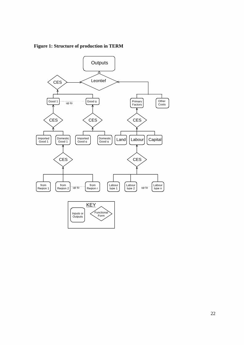
chosen to satisfy demands, which in turn reflect prices and incomes. Figure 1 shows the

production structure of each sector in the model. Starting at the bottom left-hand corner of this

figure, industry demands for intermediate inputs by region follow a constant elasticity of

substitution (CES) form, used repeatedly in the model. For example, if the price of red wine

grapes sold to red wine production in the Barossa Valley increases relative to other domestic

red wine grape sources, there will be a decrease in the Barossa-sourced proportion of red wine

9

grape purchases. Each domestic composite good is substitutable with the imported good. In

the production technology, there are potentially g composite inputs used by each industry.

Composites of each good also follow CES substitution possibilities with one another, though

weakly so. Were the parameter unsuitably large, it would imply that red wine grapes were

readily substitutable with other intermediate inputs in red wine production, which would not

be realistic - or legal.

The bottom right-hand corner of Figure 1 shows substitution between different labour types.

The labour input composite is substitutable at the next level with capital and land. The

primary factor composite, other costs, and the intermediate input composite follow Leontief or

fixed proportions technologies, with proportions determined by the output level as shown at

the top of Figure 1.

Different types of technical changes are possible within TERM. Different variables describe

primary-factor and intermediate-input-saving technical change in current production. In our

simulations, these variables are held on their base case forecast paths except for grape

production in the Barossa Valley, reflecting the assumptions of our scenarios.

3.2 Investment Investment decisions in each industry are driven by rates of return. Capital stocks depend on

past investments and depreciation. TERM allows for short-run divergences in the ratios of

actual to required rates of return from their levels in the base case forecasts. Short-run changes

in these ratios cause changes in the same direction in investment. Movements in investment

are reflected with a lag in capital stocks. These adjustments in capital stocks gradually erode

initial divergences in the rate of return ratios. In the present application, capital stocks in the

the Barossa grape sectors (and in the Rest of South Australia grape sectors in the second

scenario) are an exception: following the hypothetical Pierce's disease outbreak, grape

industry capital decreases exogenously to reflect the removal of vineyards due to Pierce's

disease. The Barossa wine sectors follow the usual investment theory of the model, so that

rising costs due to rising grape scarcity are likely to depress winery investment in our

scenarios.

10

3.3 Other final demands Each region in the model contains a representative household. Aggregate consumption is

determined via a consumption function linked to disposable income net of interest payments.

Household demands for each commodity follow a linear expenditure system, otherwise known

as the Stone-Geary or Klein-Rubin form. In addition to investors and households, the other

final users in the model are foreign buyers and the government. Exports are assumed to be

finitely elastic in the export demand equations, with typical export demand elasticities of

around -4. This is based on a derivation of export demand elasticities from import substitution

parameters as presented in Dixon and Rimmer (2002, pp. 222-225). Government spending is

assumed to be exogenous, so that policy scenarios do not result in variations in real

government spending on each commodity. An exception is in a variant of the second scenario,

in which we model compensation payments to affected grape growers: increases in national

income taxes are used to fund these payments. Unlike the single region national MONASH

model, each industry and commodity in the model is represented at the regional level. TERM

imposes a fixed exchange rate and free trade between regions, and common external tariffs. In

this sense, TERM remains a national model, rather than international. The links to foreign

markets are through the export demand equations and import supplies, which are assumed

exogenous (that is, in perfectly elastic supply), on the basis that Australia's import share of

global markets is too small to influence such prices.

3.4 The baseline forecast and policy modes TERM can be run in two modes: baseline forecasting and policy. In baseline forecasting or

control mode, it takes as inputs forecasts of macro and trade variables from organizations such

as Access Economics (2005), together with trend forecasts of demographic, technology and

consumer-preference variables. It then produces detailed baseline forecasts for industries and

regions. Our study has been supplemented by industry-specific forecasts for the grape and

wine sectors based on known vineyard plantings (Australian Bureau of Statistics, 2005b). In

policy mode, it produces deviations from baseline forecast paths in response to shocks such as

changes in government policies, technologies, world commodity prices and, in our study, pest

incursions.

11

The macroeconomic variables in the model are aggregates of sectoral activities. Therefore, if

we are to impose macroeconomic baseline forecasts on the model, such forecasts must impact

directly at the sectoral level. For example, to impose a certain change in regional real GDP to

match a given forecast, an endogenous all-industry technological change variable moves to

accommodate the target. To fit an aggregate consumption target, a consumption function

shifter is made endogenous, so that household demand for all commodities moves with the

shifter according to the household demand theory of the model.

In running the model in policy deviation mode, important indicators include the deviation in

macroeconomic variables from forecast. This implies that such variables need to be

endogenous in our deviation run. To facilitate this, following the method detailed in Dixon

and Rimmer (2002, chapter 2), when we run the policy simulation, variables such as the all-

industry technological change and consumption function shifter variables are exogenous, and

shocked by the same percentages as when they were endogenous and real GDP and aggregate

consumption exogenous in forecast. Through this method, the macroeconomic variables

become endogenous as required while we ascribe demand and supply shifts that are consistent

with the underlying forecasts of the model. The forecast and policy simulations are run

separately, year-by-year. The shocks are ascribed to the policy simulation for a given year,

based on the policy simulation database for the previous year. We report deviations in the

policy run from forecast.

3.5 Regional labour market dynamics In section 3.1, we outlined how industry demands for labour are determined. Now, we turn to

the dynamic theory of the labour market at the regional level. The regional labour market

adjustment mechanism, in levels, is given by:

1

1

1 1r r rr

tt t tr r r rt t t t

W W LSEMPWf Wf EMPf LSf

α−

−

⎛ ⎞ ⎛ ⎞ ⎛ ⎞− = − + −⎜ ⎟ ⎜ ⎟ ⎜ ⎟⎜ ⎟ ⎜ ⎟ ⎜ ⎟

⎝ ⎠ ⎝ ⎠ ⎝ ⎠ (1)

In policy mode, if the deviation shock weakens the labour market in region r and period t

relative to forecast, real wages rtW in deviation will fall relative to forecast r

tWf . In addition,

12

there will be an initial enlarged gap between labour market demand rtEMP and supply LSr

t ,

relative to forecast levels EMPf rt and LSf r

t , based on the assumption that wages adjust

slowly in the short term. In successive years, the gap between demand and supply will

gradually return to forecast through a further decline in real wages. The speed of labour

market adjustment is governed by α, a positive parameter.

The regional labour supply equation is:

( )( )

( )( )

rrrttt

r q q q qt t t t tq q

WfWLSLSf W S Wf Sf

γγ

γ γ=∑ ∑

(2)

The deviation from forecast in regional labour supply depends on the deviation in regional

relative to national real wages. In (2), ( )∑q

qt

qt SW

γ is a measure of labour responsiveness to real

wages summed across all regions, where γ is a positive parameter and S qt the share of region q

in national employment. Within this theory, should the deviation from forecast in real wages

in a region fall relative to that for national real wages, its labour supply will fall, while that in

other regions will rise. Combining (1) and (2), adjustment in a weakened labour market in a

given region will initially occur via a combination of additional unemployment and lower real

wages, with sluggish wages adjustment. Unemployment will eventually return to forecast

rates, with lower real wages. As real wages fall relative to control, the region’s labour supply

will also fall. Labour market adjustment occurs as a combination of inter-regional labour

migration and changes in regional real wage differentials within this theory.

4. The scenario

We assume that Pierce's disease affects 10 properties totalling 150 hectares. The outbreak

response necessitates complete removal of all vines on these properties, plus placing these

properties under quarantine until the disease is eliminated. The vineyards account for around 2

per cent of Barossa Valley's wine grapes. In addition, all vineyards within a 10 kilometre

radius are subjected to additional spraying to restrict the vectors of the Pierce's disease. It is

assumed that the most effective vector, the glassy winged sharpshooter, is also present in the

13

affected region. This requires spraying virtually all vineyards in the Barossa Valley. Total

additional spraying costs are estimated to be $5 million per annum, with a further $5 million

(all reported dollar figures are in Australian dollars) of R&D and administrative costs. After

five years, the pathogen is eradicated and affected properties are removed from quarantine.

The cost sharing arrangement splits the costs of disease management and compensation

(known as Owner Reimbursement Costs) to affected growers between the Australian

government (40%), the state governments (in this case that of South Australia, 40%) and

industry (20%). The amount of compensation to growers has been devised to reflect profit

losses, compensation for the depreciated value of the lost plantation (i.e., vineyards in our

example) and lost income arising from land being placed in fallow during a quarantine period.

The objective of compensation is that a grower is neither better nor worse off as a result of an

incursion response. If compensation were too high, some growers would end up better off by

earning as much as they would in the absence of an incursion, with reduced labour inputs. On

the other hand, if compensation were too low, some growers would be financially

disadvantaged by the incursion response, and may not be able to afford to remain in the

industry.

In our scenario, we assume that growers who are required to remove their vineyards are paid a

lump sum of $30,000 per hectare for the lost capital value. In addition, they are paid $8,000

per hectare for each year their vineyards are out of production. This is based on assumed

average yield of 8 tonnes per hectare and an average grape price of $1,250 per tonne, less

average costs of vineyard management and harvesting of $2,000 per hectare. The total costs of

disease management and compensation in the first year, based on 150 hectares of removed

vineyards, are $4.5 million in lost capital value, $1.2 million in annual income compensation

and $10.0 million in additional spraying and management. The total costs in the first year of

the management and compensation package are $15.7 million. The Australian and South

Australian governments fund $6.3 million each in the first year, with $3.1 million coming

from a levy on grapegrowers. Costs fall to $10.2 million in succeeding years after the initial

lump-sum payment. Once the disease has been eradicated, we assume that payments to

14

affected growers of $1.2 million continue for another five years to reflect expected income

from the now destroyed crop.

To examine the modelled economic impacts of the incursion, we turn first the industry output

results for the directly affected sectors (Table 1). The initial shrinkage in Barossa output of red

and white wine grapes raises grape prices and consequent input costs for the wine sectors in

the Barossa and other regions. Output of red wine shrinks by more than 0.2 percent in 2006

relative to the baseline forecast in both the Barossa and in the rest of South Australia, with

shrinkages in the white wine sectors of the two regions by just under 0.2 percent. That wine

outputs also fall in the rest of Australia in 2006 indicates that grape prices have risen in the

composite region, with an increasing proportion of interstate grapes being sold to Barossa

wineries for processing

Figure 2 shows the impact of the Pierce's disease incursion on wine grape producer prices in

the Barossa and in the rest of South Australia. Producer prices rise during the period of the

incursion, reflecting a greater scarcity of wine grapes within the Barossa Valley. Given that

grapes from different regions are substitutable to some extent, bad news for Barossa grapes

growers in this scenario (in which there is no threat of incursion and no additional

management costs outside the Barossa) translates into good news for grape growers

elsewhere, as Barossa wineries source grapes increasingly from outside the region. That grape

outputs persists below forecast long after Pierce's disease has been eradicated from the

Barossa Valley reflects slightly depressed investment in the wine sectors following raised

grape prices for several years.

The contribution of various sectors to the change in income in the Barossa Valley relative to

forecast is shown in Table 2. That is, the percentage change in each industry’s output is

multiplied by its share of regional income. The table includes the factor income contribution

to the deviation in real GRP from forecast for selected industries, with a separate row for

technological and tax changes. In this study, technological change includes the additional

spraying and administration costs, while the additional industry levy is an example of an

industry tax. In 2006, direct impacts dominate the change in regional income: the grape

15

sectors account for 0.64 percent out of a total income loss of 0.71 percent relative to forecast

(i.e., red grapes -0.09%, white grapes -0.12%, technological (a negative contribution) plus tax

changes (a small positive contribution) -0.43%).

By 2010, the year prior to the disease being eliminated, indirectly affected sectors make a

larger contribution to the deviation from forecast. Investment in the grape and wine sectors in

the Barossa Valley relative to forecast has fallen. In addition, a fall in aggregate consumption

relative to forecast has reduced output of the relatively income-elastic housing sector. Each of

these impacts leads to reduced output for the construction sector, whose sales consist almost

entirely of investment activity. Housing’s contribution to the deviation in regional income

from forecast is now -0.09%, while that of construction is -0.14%.

Aggregate consumption falls proportionally more than real GRP in the Barossa Valley, being

1.75 per cent below forecast in 2010 compared with a real GRP fall of less than one per cent.

In part, this reflects the negative impact of reduced regional income on non-traded sector

prices, including housing. Sectors relatively intensive in sales of goods traded out of the

region are affected proportionally less. The Barossa Valley therefore has a real depreciation

relative to forecast during the incursion, inducing an increase in net inter-regional and

international exports as a share of real GRP, while regional domestic absorption decreases as a

share of real GRP. Since government spending, one of the components of domestic

absorption, is fixed by assumption, investment and consumption fall proportionally more than

the overall fall in domestic absorption.

In 2015, although Pierce’s disease has been eradicated and investment in the region has been

restored almost to baseline forecast levels (Figure 3), replanted vineyards are not yet fully

bearing. Therefore, the grape sectors still make a substantial negative contribution to regional

income relative to forecast (although most of the negative technical change contribution has

been eliminated). The contribution of housing remains negative, recovering slowly in

subsequent years – housing’s contribution to regional GDP is -0.09 per cent relative to

forecast in 2010 and 2015, and still 0.03 per cent below forecast in 2025 (Table 2).

16

Figure 4 shows the impact of the incursion on the Barossa Valley's labour market, following

the theory of labour market adjustment outlined in equations (1) and (2). The initial

production loss wipes almost 0.3 per cent off the region's employment, equivalent to 80 jobs.

Although additional spraying in the Barossa Valley creates some jobs, as does grubbing out

vineyards (a one-off, relatively capital-intensive activity), these are more than offset by the

negative employment effects. These include pruning and grape-picking that are no longer

undertaken once vineyards have been removed. Placing land in quarantine and falling rates of

return in Barossa vineyards discourage investment (a relatively labour-intensive activity) in

vineyards, wineries and housing, so that employment continues to fall after the first year

(2006) in which there is a response to the incursion. Real wages continue to fall until the pest

has been eradicated, as labour supply remains above employment in this period. Following the

eradication of Pierce's disease in 2011, after employment has bottomed out at 0.45 per cent or

120 jobs below forecast in the Barossa Valley, the region's employment thereafter rises above

forecast very slightly due to catch-up investment. Real wages slowly return towards the

baseline, but are not fully restored, reflecting our assumption that although yields recover

within 5 years of replanting, grape quality in new vineyards does not match that of the

vineyards they replaced. In addition, the incursion depresses investment in the Barossa

Valley's wine sectors, so that wine processing capacity remains slightly below forecast at the

end of the simulation period.

South Australia accounts for no more 6.5 per cent of national economic activity, but contains

around half the nation's grape and wine production (including that of the Barossa Valley). In

the rest of South Australia (i.e., excluding Barossa), there are gains for the wine grape sectors

due to rising scarcity in the Barossa region, but these increase the production costs of wineries

in the rest of the state. There are very small adverse employment consequences for the rest of

the state, due to rising costs during the incursion and consequent slower-than-forecast

investment in wine sectors during and after the incursion. After 2011, employment relative to

forecast falls slightly, due to labour being drawn into the Barossa during the recovery phase,

but bottoms out only 0.005 per cent or 35 jobs below forecast in 2017 (Figure 5).

17

4.1 Welfare impacts and sensitivity analysis

The discounted net present value of the national welfare loss, calculated as the deviation in

national aggregation consumption from the baseline forecast, is $135 million. A similar

calculation, confined to the deviation in the Barossa’s real GRP from forecast (see Table 2 and

Figure 5), reveals a discounted regional income loss of $120 million. Nationally, the

discounted income loss is only $110 million. This implies higher than forecast income outside

the Barossa, reflecting migration out of the region during the incursion. The difference

between the discounted national consumption and income losses reflects in part additional

investment required to replant vineyards. It also reflects a very weak terms-of-trade

deterioration arising from the incursion that reduces consumption’s share of national income

slightly.

The welfare result depends to some extent on assumed rate of adjustment in the labour market.

This depends on two parameters, α in equation (1), governing regional real wage adjustment,

and γ in equation (2), governing inter-regional migration. The default setting for α is 0.5

which implies that half of the gap between regional labour demand and supply will be

eliminated in the following year via real wages adjustment. Raising this parameter to 0.9

implies that most real wages adjustment will occur within a single year, thereby lessening job

losses when the labour market weakens. Raising γ from the default setting of 0.2 to 0.5

implies more rapid inter-regional migration in response to regional labour market changes.

The scenario was run again three times, with α set to 0.9, γ set to 0.5 and with both parameters

at the higher settings. In each case, the net present value of the welfare loss diminished

slightly, to around $120 million (relative to $135 million with the default parameters),

indicating that employment losses play only a small part in the overall welfare impact of the

incursion.

5. Conclusion

This paper has analysed the economic impacts of a hypothetical incursion of Pierce's disease

in the Barossa Valley region of South Australia. We assume Pierce's disease is controlled

18

within 5 years with limited damage at the regional level. Our scenario assumed that industry

and public funding were used in a successful campaign to eradicate the pathogen. The success

of such a campaign would depend on early detection and thus an industry culture of early

reporting, followed by an active field-based eradication campaign. Even in this relatively

moderate incursion response, the welfare loss was $135 million in discounted net present

value terms.

Perhaps the main issue in allocating resources to preventive measures is that these need not be

incursion-specific. To the extent that resources directed at disease prevention can apply to a

number of diseases across a range of crops, an appropriate level of preventive resources would

reflect expected welfare losses, that is, the probability of each incursion multiplied by

estimated welfare losses summed across all possible incursions. While the expected welfare

loss may be sufficient to justify some preventive or contingency measures specifically for

Pierce’s disease, the summed expected welfare losses across many possible significant exotic

threats are more substantial: Plant Health Australia usually deals with a number of minor

incursions each year and a major incursion every year or two in the crops covered by its

partner organisations. This warrants generic risk mitigation and contingency measures to

minimise the likelihood of entry and maximise the potential for successful eradication

campaigns in the future.

The multi-regional framework of our dynamic model, with its theory of imperfect, regional

labour market adjustment would be useful in applications, for example, to regions within the

European Union. There may concerns among farmers in Western Europe that pest and disease

incursions could affect specific agricultural regions, such as the historic wine producing

regions in parts of Europe. Moreover, interest in policy debate is increasingly on regional

rather than national implications. Development of a database of Europe for relevant policy

analysis within TERM is feasible, following a methodology outlined in Horridge et al. (2005).

19

References Access Economics (2005). Business Outlook. March, Canberra. Anderson, K and Norman, D. (2003). Global Wine Production, Consumption and Trade, 1961 to 2001. Centre for International Economic Studies: The University of Adelaide.

Australian Bureau of Statistics (2005a). Australian national accounts, State accounts. ABS catalogue no. 5220.0.

Australian Bureau of Statistics (2005b). Australian Wine and Grape Industry. ABS catalogue no. 1329.0.

Australian Wine and Brandy Corporation (2006). Australian Regional Crush Survey Online, http://www.awbc.com.au/ARWCS/areaoutcomes.asp (accessed 24 March, 2006).

Dixon P.B. and Rimmer, M.T. (2002). Dynamic General Equilibrium Modelling for Forecasting and Policy: a Practical Guide and Documentation of MONASH. Contributions to Economic Analysis 256, North-Holland Publishing Company, Amsterdam. Dixon P.B., Menon, J. and Rimmer, M.T. (2000). Changes in technology and preferences: a general equilibrium explanation of rapid growth in trade. Australian Economic Papers 39: 33-55. Hoddle, M.S. (2002). Progress made in understanding GWSS including its natural enemies and impact. The Australian and New Zealand Grapegrower and Winemaker 459: 17-22. Hoddle, M.S. (2004). The potential adventive geographic range of glassy-winged sharpshooter, Homalodisca coagulata and the grape pathogen Xylella fastidiosa: implications for California and other grape growing regions of the world. Crop Protection, 23: 691-699. Horridge, M., Madden, J. and Wittwer, G. (2005). Using a highly disaggregated multi-regional single-country model to analyse the impacts of the 2002-03 drought on Australia. Journal of Policy Modelling 27: 285-308. Luck, J., Traicevski, V., Mann, R., Moran, J. and Merriman, P. (2001). The potential for the establishment of Pierce’s disease in Australian grapevines. Final Report to Grape and Wine Research and Development Corporation DNR00/1. Luck, J., Letham, D., McKirdy, S. and Brown, B. (2002). Pierce's Disease and the Glassy-winged sharpshooter-Understanding the threat and minimising the risks. The Australian and New Zealand Grapegrower and Winemaker 462: 22-26. Mumford, J.D. (2002). Economic issues related to quarantine in international trade. European Review of Agricultural Economics 29(3): 329-348.

20

Varela, L.G., Smith, R.J. and Phillips, P.A. (2001). Pierce’s disease. University of California: Agriculture and Natural Resources. Wittwer, G., McKirdy, S. and Wilson, R. (2005). The regional economic impacts of a plant disease incursion using a general equilibrium approach. Australian Journal of Agricultural and Resource Economics 49: 75-89. WTO (World Trade Organization) (1994). Agreement on the Application of Sanitary and Phytosanitary Measures. Geneva: WTO.

21

Table 1: Outputs of grape and wine sectors (% deviation from baseline forecast) Barossa 2006 2010 2015 2020 2025 Red grapes -3.69 -3.58 -2.41 -1.53 -0.94 White grapes -2.13 -2.09 -2.09 -1.16 -0.59 Red Wine -0.28 -0.26 -0.41 -0.42 -0.38 White Wine -0.17 -0.17 -0.37 -0.41 -0.34 Construction -0.01 -0.97 -0.17 0.06 -0.04 Trade -0.12 -0.2 0.04 0.03 -0.02 Rest of Sth Aust 2006 2010 2015 2020 2025 Red grapes 0.16 0.07 -0.18 -0.23 -0.26 White grapes -0.03 -0.12 -0.21 -0.25 -0.27 Red Wine -0.24 -0.36 -0.47 -0.38 -0.3 White Wine -0.16 -0.29 -0.35 -0.29 -0.24 Rest of Aust 2006 2010 2015 2020 2025 Red grapes 0.1 0.02 -0.19 -0.23 -0.24 White grapes -0.04 -0.14 -0.22 -0.23 -0.23 Red Wine -0.19 -0.33 -0.45 -0.37 -0.31 White Wine -0.16 -0.28 -0.36 -0.29 -0.26

Table 2: Contribution of selected sectors to Barossa Valley’s real GRP (% deviation from baseline forecast) 2006 2010 2015 2020 2025 Red grapes -0.09 -0.12 -0.10 -0.08 -0.08 White grapes -0.12 -0.15 -0.17 -0.14 -0.12 Agricultural services 0.01 0.02 0.01 0.00 0.00 Red Wine -0.02 -0.02 -0.03 -0.03 -0.03 White Wine -0.01 -0.01 -0.02 -0.03 -0.02 Construction -0.01 -0.14 -0.03 0.02 -0.01 Trade -0.02 -0.01 0.02 0.02 0.02 Housing -0.01 -0.09 -0.09 -0.05 -0.03 Other sectors -0.03 0.07 0.16 0.14 0.13 Total -0.28 -0.45 -0.25 -0.14 -0.14 Tech. change + indirect taxes -0.43 -0.45 0.08 0.08 0.06 Real GRP -0.71 -0.90 -0.17 -0.07 -0.08

22

Figure 1: Structure of production in TERM

up to

up to up tofrom

Region r from

Region 2

CES

from Region 1

KEY Inputs or Outputs

FunctionalForm

CES

CESCES CES

Labourtype n

Labourtype 2

Labourtype 1

Capital Labour Land

PrimaryFactors

DomesticGood g

Imported Good g

Domestic Good 1

Imported Good 1

Good g Good 1

Leontief

Outputs

OtherCosts

CES

23

Figure 2: Impact of the incursion on wine grape prices in the Barossa Valley and the rest of South Australia (% deviation from baseline forecast)

0.0

0.5

1.0

1.5

2.0

2.5

3.0

2005 2008 2011 2014 2017 2020 2023

Red grapes, rest of Sth Aust

Red grapes, Barossa

White grapes, Barossa

White grapes, rest of Sth Aust

Figure 3: Impact of the incursion on Barossa Valley's aggregate consumption and investment (% deviation from baseline forecast)

-2

-1.5

-1

-0.5

0

0.5

1

2005 2008 2011 2014 2017 2020 2023

Aggregate consumption -- Barossa

Aggregate investment -- Barossa

24

Figure 4: Impact of the incursion on the Barossa Valley's labour supply, employment and real wages (% deviation from baseline forecast)

-1

-0.8

-0.6

-0.4

-0.2

0

0.2

2005 2008 2011 2014 2017 2020 2023

Real wage -- Barossa

Labour supply -- Barossa

Employment -- Barossa

Figure 5: Impact of the incursion on the Rest of South Australia's labour supply, employment and real wages (% deviation from baseline forecast)

-0.016

-0.014

-0.012

-0.01

-0.008

-0.006

-0.004

-0.002

0

0.002

2005 2008 2011 2014 2017 2020 2023

Employment -- Rest of SA

Real wage-- Rest of SA

Labour supply-- Rest of SA

25

Appendix: a no-recovery scenario

Available evidence from California indicates that Pierce’s disease could be so far advanced on

detection that no recovery of vineyards in the affected region is possible. In this alternative

scenario, the vector for the of Pierce's disease is not brought under control. This scenario

depicts a policy response in which the focus is entirely on structural assistance into other

economic activities, without any effort being devoted to disease eradication. The decision not

to attempt to eradicate the disease may be due to a judgment by industry and statutory bodies

that the outbreak is too widespread when detected to be manageable. The initial outbreak in

this scenario results in one tenth of the region's vineyards being removed in 2006. Thereafter,

in this scenario, vineyards in the Barossa Valley are successively removed over time as

Pierce's disease spreads through the region. At the end of the simulation period in the year

2025, four fifths of the Barossa Valley's vineyards have been destroyed by Pierce's disease. At

the same time, the disease had spread to other vineyard districts in South Australia (the

outbreak becoming apparent a year later than in the Barossa), particularly to the south of the

Barossa, given the expectation that the vector would travel relatively long distances with hot

northerly spring and summer winds. In this hypothetical case, the incursion is too widespread

for the cost sharing arrangements to apply. All that growers can expect is some government

funding to assist in movement into other industries.

The outcomes for wine grape prices and outputs differ markedly between the Barossa, the rest

of South Australia and the rest of Australia. In the Barossa, in which four-fifths of output is

wiped out by 2025, output prices have not quite doubled by then, indicating substantial losses

in regional grape revenue (Figure A1). In the rest of South Australia, which is a net exporter

of grapes to the Barossa prior to the incursion, grape revenue increases relative to forecast

even though some vineyards are destroyed by Pierce's disease. For example, by 2025, red

wine grape prices have increased by 25 per cent, coupled with an output decline of 8 per cent,

indicating revenue increases relative to forecast (Figure A2). It follows that growers outside

South Australia benefit from higher prices, induced by a degree of substitutability with South

Australian grapes, without suffering the output reducing impacts of the disease. Indeed, higher

rates of return to vineyard investment interstate, induced by growing scarcity in South

26

Australia, contribute to a rise in grape output in the rest of Australia relative to forecast

(Figure A3).

Figure A4 reveals the impact of this pessimistic scenario on the Barossa Valley's labour

market. Due to ongoing vineyard removals, real wages are still falling further relative to

forecast in 2025 in the ever-weakening labour market. Real wages have fallen relative to

forecast by 15 per cent in 2025. At the same time, employment has fallen by around 5 per cent

or 1,500 jobs. In addition, there has been a net migration to other regions, reflected in falling

labour supply, of 3 per cent or 900 workers (45 workers per year), and an increase in jobless

in the Barossa Valley relative to control of 600 by 2025. In the larger economy of the rest of

South Australia, labour supply has fallen relative to forecast by 0.04 per cent in 2025,

amounting to outward net migration of 280 workers. Unemployment has worsened, as the

number employed in the region has fallen by 700 relative to forecast. The fall in wages in

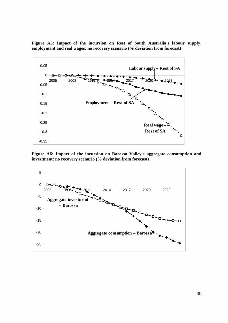
South Australia is just over 0.3 per cent relative to forecast by 2025.

The macroeconomic impacts on the expenditure and income sides respectively for the Barossa

Valley are shown in figures A6 and A7. Aggregate investment and consumption in the region

both fall continuously relative to forecast, by 15 per cent and 25 per cent respectively in 2025

(Figure A6). The decline in aggregate investment tracks real GRP, which is 14 per cent below

control in 2025 (Figure A7). As in the first scenario, the percentage decline in aggregate

consumption is larger than real GRP, reflecting both the impact of a real devaluation on

regional domestic absorption and the assumption that aggregate government spending

(excluding adjustment assistance to growers) in the region has not changed relative to

forecast. As an indicator the region’s real devaluation, the sector with the largest price decline

is housing: prices in this non-traded sector have fallen 30 per cent relative to forecast by 2025,

compared with a decline in the region’s CPI (which includes traded goods) of 6.5 per cent.

In the rest of South Australia, in which grapes make a relatively small contribution to the

economy, the economy slowly declines relative to forecast. Initially, in 2006 before the

disease has affected vineyard outputs outside the Barossa Valley, aggregate consumption in

the rest of the state rises relative to forecast (Figure A8). This is because the rise in grape

27

prices, without any offsetting output loss in the region, improves the region’s terms-of-trade

temporarily, so that aggregate consumption as a share of GRP rises. In subsequent years,

despite wine grape revenues in the region increasing, production costs for wineries rise,

worsening as vineyard removals continue, leading to declines in winery investment. In both

the Barossa Valley and the rest of South Australia, aggregate capital stocks decrease

proportionally more than labour (Figures 13 and 15). This is because we assume regional

wages can adjust downwards in response to a regional economic downturn, whereas rates of

return on capital are determined in international markets, and therefore not likely to persist

below forecast rates of return in the long run. With real wages falling relative to capital

rentals, the labour to capital ratio in industries in these regions must increase.

We assume in this scenario that after a two year period of quarantine, former vineyards are

moved into other farming activities. Some land switched to other horticultural production may

earn returns per hectare similar to those earned by vineyards prior to the outbreak. Through

lack of access to irrigation water and insufficient rainfall for other horticulture, other land

grubbed of vineyards is suitable only for broadacre activity. Overall, the returns from

alternative land uses per hectare are lower than for vineyards. Moreover, grubbed vineyards

represent lost capital that has a marked effect on income earning capacity. The value of lost

vineyards combined with lost employment make substantial contributions to overall welfare

losses. In this scenario, the discounted net present value of welfare losses is $4.2 billion by

2025, and still growing as a consequence of ongoing vineyard removals and ongoing

disruption to the labour market.

28

Figure A1: Impact of the incursion on the Barossa Valley's wine grape outputs and producer prices: no recovery scenario (% deviation from forecast)

-80.0

-60.0

-40.0

-20.0

0.0

20.0

40.0

60.0

80.0

100.0

2005 2008 2011 2014 2017 2020 2023

White grapes, price output, Barossa

Red grapes, price -- Barossa

Red grapes, output -- Barossa

Figure A2: Impact of the incursion on Rest of South Australia's wine grape outputs and producer prices: no recovery scenario (% deviation from forecast)

-20

-15

-10

-5

0

5

10

15

20

25

30

35

2005 2008 2011 2014 2017 2020 2023

Red grapes, price, Rest of SA

Red grapes, output, Rest of SA

White grapes, priceoutput -- Rest of SA

29

Figure A3: Impact of the incursion on Rest of Australia's wine grape outputs and producer prices: no recovery scenario (% deviation from forecast)

0

2

4

6

8

10

12

14

16

18

2005 2008 2011 2014 2017 2020 2023

White grapes, price -- Rest of Aust

Red grapes, price output -- Rest of Aust

White grapes,output -- Rest of Aust

Figure A4: Impact of the incursion on Barossa Valley's labour supply, employment and real wages: no recovery scenario (% deviation from forecast)

-18

-16

-14

-12

-10

-8

-6

-4

-2

02005 2009 2013 2017 2021 2025

Real wage -- Barossa

Labour supply -- Barossa

Employment -- Barossa

30

Figure A5: Impact of the incursion on Rest of South Australia's labour supply, employment and real wages: no recovery scenario (% deviation from forecast)

-0.35

-0.3

-0.25

-0.2

-0.15

-0.1

-0.05

0

0.05

2005 2008 2011 2014 2017 2020 2023

Employment -- Rest of SA

Real wage-- Rest of SA

Labour supply-- Rest of SA

Figure A6: Impact of the incursion on Barossa Valley's aggregate consumption and investment: no recovery scenario (% deviation from forecast)

-25

-20

-15

-10

-5

0

5

2005 2008 2011 2014 2017 2020 2023

Aggregate consumption -- Barossa

Aggregate investment -- Barossa

31

Figure A7: Impact of the incursion on Barossa Valley's aggregate capital, labour and real GRP: no recovery scenario s (% deviation from forecast)

-18

-16

-14

-12

-10

-8

-6

-4

-2

02005 2009 2013 2017 2021 2025

Employment -- Barossa

Real GRP -- Barossa

Capital stocks -- Barossa

Figure A8: Impact of the incursion on Rest of South Australia's aggregate consumption and investment: no recovery scenario (% deviation from forecast)

-0.45

-0.4

-0.35

-0.3

-0.25

-0.2

-0.15

-0.1

-0.05

0

0.05

2005 2008 2011 2014 2017 2020 2023Aggregate consumption --

Rest of SA

Aggregate investment --Rest of SA

32

Figure A9: Impact of the incursion on Rest of South Australia's aggregate capital, labour and real GRP: no recovery scenario (% deviation from forecast)

-0.7

-0.6

-0.5

-0.4

-0.3

-0.2

-0.1

0

0.1

2005 2008 2011 2014 2017 2020 2023

Capital stocks -- Rest of SA

Real GDP -- Rest of SA

Aggregate employment -- Rest of SA