analysis and design optimization of laminated composite
TRANSCRIPT
Analysis and Design Optimization
of Laminated Composite Structures
using Symbolic Computation
Evan Summers
Submitted in fulfilment of the academic requirements for the degree of
Doctor of Philosophy in the Department of Mechanical Engineering
at University of Natal.
Durban, South Africa October 1994

To Ben Coughlan
Abstract
The present study involves the analysis and design optimization of thin and thick
laminated composite structures using symholic computation.
The fibre angle and wall thickness of balanced and unbalanced thin composite pres
sure vessels are optimized subject to a strength criterion in order to maximise in
ternal pressure or minimise weight , and the effects of axial and torsional forces on
the optimum design are investigated.
Special purpose symbolic computation routines are developed in the C programming
language for the transformation of coordinate axes, failure analysis and the calcu
lation of design sensitivities. In the study of thin-walled laminated structures, the
analytical expression for the thickness of a laminate under in-plane loading and its
sensitivity with respect to the fibre orientation are determined in terms of the fibre
orientation using symbolic computation. In the design optimization of thin com
posite pressure vessels, the computational efficiency of the optimization algorithm
is improved via symbolic computation.
A new higher-order theory which includes the effects of transverse shear and nor
mal deformation is developed for the analysis of laminated composite plates and
shells with transversely isotropic layers. The Mathematica symbolic computation
package is employed for obtaining analytical and numerical results on the basis of
the higher-order theory. It is observed that these numerical results are in excellent
agreement with exact three-dimensional elasticity solutions. The computational ef
ficiency of optimization algorithms is important and therefore special purpose sym
bolic computation routines are developed in the C programming language for the
design optimization of thick laminated structures based on the higher-order theory.
Three optimal design problems for thick laminated sandwich plates are considered,
namely, the minimum weight, minimum deflection and minimum stress design. In
the minimum weight problem, the core thickness and the fibre content of the surface
layers are optimally determined by using equations of micromechanics to express the
elastic constants. In the minimum deflection problem, the thicknesses of the surface
layers are chosen as the design variables. In the minimum stress problem, the relative
thicknesses of the layers are computed such that the maximum normal stress will
be minimized. It is shown that this design analysis cannot be performed using a
classical or shear-deformable theory for the thick panels under consideration due to
the substantial effect of normal deformation on the design variables.
/A6cTpaKT

A6CTPaKT
HaCTOxw;ee lICCJIe,ll;OBaHlIe BKJIIO"tIaeT B ce65I OIITlIM1I3aD;lIIO TOHKlIX 11 TOJICThlX CJIo
lICThlX KOMII031ITHhlX KOHCTPYKD;lIH lICIIOJIb3Y5I ClIMBOJIbHhlH MeTO,ll; Bhl"tIlICJIeHlI5I.
IIpe,ll;MeTOM OIITlIM1I3aD;1I1I, C lICIIOJIb30BaHlIeM KplITeplI5I IIPO"tIHOCTlI, 5IBJI5IIOTC5I yrOJI
apMlIpOBaHlI5I BOJIOKOH 11 TOJIID;lIHa CTeHKlI C6aJIaHClIpOBaHHhlX 11 Hec6aJIaHClIpOBaH
HbIX TOHKlIX KOMII031ITHhlX COCY,ll;OB ,ll;aBJIeHlI5I, B pe3YJIbTaTe "tIerO OIIpe,ll;eJI5IeTC5I
MaKClIMaJIbHOe ,ll;OIIYCTlIMOe BHYTpeHHee ,ll;aBJIeHlIe lIJIlI MlIHlIMaJIbHhli BeC. 3<p<peKT
IIPO,ll;OJIbHbIX 11 KPYTXW;lIX ClIJI Y"tIlITbIBaeTC5I IIplI OIITlIM1I3aD;1I1I IIapaMeTpOB KOH
CTPYKD;lIH.
nJI5I IIpe06pa.30BaHlI5I KOOp,ll;lIHa T, aHaJI1I3a pa.3pymeHlI5I 11 OD;eHKlI "tIYBCTBlITeJIb
HOCTlI KOHCTPYKD;lIH IIplI OIITlIMaJIbHOM IIpoeKTlIpOBaHlIlI pa.3pa6oTaH MeTO,ll; CIIe
D;lIaJIbHbIX ClIMBOJIbHhlX BbI"tIlICJIeHlIH C lICIIOJIb30BaHlIeM aJIrOplITMlI"tIeCKOrO 5I3bIKa
IIporpaMMlIpOBaHlI5I C. lIcIIOJIb3Y5I IIpoD;e,ll;Ypy ClIMBOJIbHOrO BbI"tIlICJIeHlI5I IIplI HC
CJIe,ll;OBaHlIlI TOHKOCTeHHhlX CJIOlICTbIX KOHCTPYKD;lIH 6hlJIO IIOJIY"tIeHO aHaJIHTlIlleCKoe
BbIpa2KeHlIe ,ll;JI5I OIIpe,ll;erreHlI5I TOJIID;lIHhl CJI05I IIplI HarpY2KeHlIlI B IIJIaHe 11 ee "tIYB
CTBlITeJIbHOCTb B 3aBlIClIMOCTlI OT yrJIa apMlIpOBaHlI5I. Bhl"tIlICJIlITeJIbHaK 3<p<peK
TlIBHOCTb aJIroplITMa OIITlIM1I3aD;1I1I IIplI ,ll;1I3aHHe TOHKlIX KOMII031ITHbIX COCY,ll;OB
,ll;aBJIeHlI5I 3Ha"tIlITeJIbHO YJIyqmeHa 6JIaro,ll;ap5I lICIIOJIb30BaHlIIO MeTO,ll;a ClIMBOJIbHbIX
BhllllICJIeHlIH CIIeD;lIaJIbHoro Ha.3Ha"tIeHlI5I.
Pa.3pa6oTaHa HOBaK YTO"tIHeHHaK HeKJIaCClIlleCKaK TeOplI5I YlllITbIBaIOlI(aK 3<p<peKT IIo
IIepe"tIHOrO C,ll;BlIra H 062KaTlI5I ,ll;JI5I aHaJI1I3a CJIOlICTbIX KOMII031ITHbIX IIJIaCTlIH 11 060-
JIO"tIeK C TpaHCBepCaJIbHO-1I30TPOIIHbIMlI CJI05IMlI. ClIMBOJIbHhlH 5I3hlK IIporpaMMlI
pOBaHlI5I Mathematica lICIIOJIb3yeTCjI ,ll;JI5I IIOJIY"tIeHlI5I aHaJIHTlIlleCKlIX H "tIHCJIeHHbIX
pe3YJIbTaTOB Ha OCHOBe YTO"tIHeHHOH HeKJIaCClI"tIeCKOH Te0PlIlI. IIoKa.3aHo, lITO lllI
CJIeHHhle pe3YJIbTaThl IIpeKpacHo CXO,ll;5ITC5I C TOllHhlM TpexMepHhlM yIIpyrHM peme
HlIeM. BbI"tIlICJIlITeJIbHaK 3cpcpeKTlIBHocTb aJIroplITMa OIITlIM1I3aD;1I1I OlleHb Ba2KHa
11 II03TOMY ,ll;JI5I OIITlIM1I3aD;1I1I TOJICThlX CJIOlICTbIX KOHCTPYKD;HH 6hlJIa pa.3pa6oTaHa
OCHOBaHHaK Ha YTOllHeHHoH HeKJIaCClIllecKoH TeOplIlI IIpOD;e,ll;ypa ClIMBOJIbHOro Me
TO,ll;a CIIeD;lIaJIbHoro Ha.3Ha"tIeHlI5I C lICIIOJIb30BaHlIeM arrroplITMlIllecKoro 5I3bIKa C.
PaCCMOTpeHhl TplI OIITlIM1I3aD;1I0HHhle 3a,ll;a"tI1I ,ll;JI5I TOJICThlX TpeXCJIOHHbIX IIJIlIT, a
lIMeHHO, ,ll;1I3aHH MlIHlIMaJIbHOro Beca, MlIHlIMaJIbHhlX ,ll;e<popMaD;lIH 11 MlIHlIMaJIbHhlX
HaIIpjl2KeHlIH. IIPlI IIo.n6ope OIITlIMaJIbHOro Beca TOJIID;lIHa 3aIIOJIHlITeJI5I 11 xapaK
TePlICTlIKlI BOJIOKOH BHemHlIX CJIOeB OIIpe,ll;eJI5IIOTC5I lICIIOJIb3Y5I ypaBHeHlI5I MlIKpo
MexaHlIKlI KOTOphle OIIpe,ll;eJI5IIOT 3Ha"tIeHlIe yIIpyrlIx KOHCTaHT. IIPlI paCCMOTpeHlIlI
3a,ll;a"tI1I MlIHlIMaJIbHhlX .ll:e<popMaD;lIH TOJIlI(lIHhl BHemHlIX CJIOeB Bhl61IpaIOTC5I B Ka-
11

"tJeCTBe nepeMeHHhIX. PaCCMaTpHBaJI 3a.n;a"tJY MHHHMaJIbHhIX HanpK2KeHHH OTHOCH
TeJIbHhIe TOJIIIJ;HHhI crroeB BhI"tJHCJIKIOTCK TaK, "tJTOOhI MaKCHMaJIbHOe HOpMaJIbHOe
HanpK2KeHHe 6hIJIO MHHHMH3HpOBaHO. IIoKa3aHo,"tJTO H3-3a 3Ha"tJHTeJIbHOro BJIHKHHK
062KaTHK Ha nepeMeHHhIe OnTHMH3a~HH 3TOT .n;H3aHH He M02KeT 6hITb ocymecTBJIeH
HCnOJIb3YK KJIaCCH"tJeCKYIO HJIH C.n;BHroBYIO .n;e<l>opMa~HOHHYIO TeOpHIO npH paCCMO
TpeHHH TOJICThIX nJIHT.
III
Declaration
I declare that this dissertation is my own unaided work except where due acknow
ledgement is made to others. This dissertation is being submitted for the Degree
of Doctor of Philosophy to the University of Natal, Durban, and has not been
submitted previously for any other degree or examination.
Evan Summers October 1994
IV

Acknowledgements
I express my gratitude to my supervisors, Professors Sarp Adali and Viktor Veri
jenko, for their guidance and encouragement; to their collaborator, Professor V. G.
Piskunov, for his contributions; and to my colleague Pavel Tabakov for his support
and encouragement.
Financial assistance from the Foundation of Research Development of South Africa
is gratefully acknowledged.
v
Contents
Abstract I
A6cTpaKT I
Declaration IV
Acknowledgements v
Contents VI
Nomenclature: Thin-walled structures Xl
Nomenclature: Higher-order theory .. Xll
List of Figures XllI
List of Tables . XVI
1 Introduction 1
1.1 Overview. 1
1.2 Symbolic Computation 3
1.3 Optimization of Thin-Walled Structures ............ . ... 4
VI
1.4 Higher-Order Theory for Thick Plates and Shells 5
1.5 Optimization of Thick Structures . . . . . . . . . 5
2 Optimization of Thin Walled Structures using Special Purpose Sym-
bolic Computation 7
2.1 Introduction . . 7
2.2 Literature Review . 8
2.3 Laminate under In-plane Load. 9
2.3.1 Basic Equations . . . 9
2.3.2 Design Optimization 11
2.4 Special purpose symbolic computation 12
2.4.1 Data Storage .... 12
2.4.2 Symbolic Processing 13
2.4.3 Matrix Algebra 15
2.5 Method of Solution 16
2.5.1 Program. 17
2.5.2 Results .. 22
2.6 Laminated Pressure Vessels 24
2.6.1 Basic Equations . . . 25
2.6.2 Problem 2.1: Design for Maximum Internal Pressure 26
2.6.3 Problem 2.2: Design for Minimum Weight 29
2.7 Conclusions ... . .... . ............ 40
3 Derivation of a Higher-Order Theory for Thick Laminated Plates and Shells 42
Vll
3.1 Introduction . . . · ............ 42
3.2 Literature Survey · ............ 43
3.3 Basic Equations . .......................... 44
3.4 Higher-Order Theory. . ................. 50
3.5 Equilibrium & Boundary Conditions .................. 53
3.6 Conclusions . . . . . . . . . . . . . . . . . . . . . . . . . . . . . . .. 62
4 Implementation of the Higher-Order Theory using Symbolic Com-
putation 63
4.1 Introduction . ............ 63
4.2 Basic Equations and Some Analytical Solutions . . . . . . . . . . .. 64
4.3 Implementation using Mathematica . . . . . . . . . . . . . . . . . .. 69
4.3.1 Derivation of Distribution Functions .............. 70
4.3.2 Derivation of Integrated Stiffnesses . . . . . . . . . . . . . .. 76
4.3.3 System of Governing Equations 79
4.3.4 Stresses and Strains . 83
4.4 Homogeneous Shell . . . . . 85 .
4.5 Special Purpose Symbolic Computation . 88
4.5.1 Symbols ... 89
4.5.2 Power Series . .......................... ........ 90
4.5.3 Symbolic Processing 90
4.5.4 Application to Higher-Order Theory 92
4.5.5 Symbolic Results ........................ 94
4.6 Numerical Results. . . . ........................ · .......... " 96
VIll
4.6.1 Isotropic Plates . . . . . . .. 96
4.6.2 Transversely Isotropic Plates . 97
4.6.3 Heterogeneous Plates 98
4.6.4 Sandwich Plates . 98
4.6.5 Isotropic Shells · 101
4.6.6 Laminated Shells · 102
4.7 Conclusions . . . . . . . . . . . . . . . ..... . . . . . ... . . · 111
5 Optimization of Thick Sandwich Plates based on Higher-Order
Theory 113
5.1 Introduction . · 113
5.2 Literature survey · 115
5.3 Software .... · 115
5.3.1 Symbols · 116
5.3.2 Distribution Functions · 116
5.3.3 Integrated Stiffnesses · 117
5.3.4 Trigonometric Series · 118
5.4 Optimal Design Problems · 119
5.4.1 Minimum Weight Design . · 119
5.4.2 Minimum Deflection Design · 121
5.4.3 Minimum Stress Design · 122
5.5 Numerical Results ........ · 123
5.5.1 Minimum Weight Design . · 123
5.5.2 Minimum Deflection Design · 124
IX
5.5.3 Minimum Stress Design
5.6 Conclusions . . . . . . . . . . .
6 Conclusions
6.1 Overview.
6.2 Symbolic Computation
6.3 Optimization of Thin Pressure Vessels
6.4 Higher-Order Theory ......... .
6.5
6.6
Optimization of Thick Sandwich Plates
Recommendations for Future Work . .
Bibliography
Appendix A. Symbolic Results from Mathematica
Appendix B. Routines for Trigonometric Series
Appendix C. Routines for Piecewise Integrals
Appendix D. Routines for Higher-Order Theory
x
· 126
· 155
157
· 157
· 158
· 159
· 160
· 160
· 162
163
171
176
195
207
k = l, ... ,n
(h x,<p,z R
P T
F
Pmax
Her
Hmin
Wmin
Qij
Qij
El,E2
VI, V2
0'1, 0'2, T12
c1, C2, C12
Nomenclature
1. Thin-walled structures
Layer number
Orthogonal coordinates
Force resultants
Normal and shear strains
Fibre angle of the k-th layer
Cylindrical coordinates
Mean Radius
Internal pressure of a pressure vessel
Torque
Axial force
Optimal fibre angle
Burst pressure
Maximum internal pressure
Laminate thickness at failure
Minimum thickness
Minimum weight
Stiffness coefficients
Reduced stiffness coefficients
Moduli of elasticity in the material coordinate system
Poisson's ratios in the material coordinate system
Stress components in the material coordinate system
Strain components in the material coordinate system
Xl
Nomenclature
2. Higher-order theory for thick plates and shells
Xl, X2, Z
X=(XI,X2)
ku, k22
k = 1, ... ,n
Ek,vk,Gk
Ul(X), U2(X), w(x) Xl(X)
X2(X) q+(x),q-(x)
(k) (k) (k) U1 ,U2 ,U3
(}:qk(Z), <pqk(Z), tPgk(Z)
O"u, 0"12, 0"22
0"13,0"23
0"33
EOk,vOk,
i111k,i112k,i113k,i133k
Curvilinear orthogonal coordinates
Orthogonal coordinate pair
Curvatures of a shell
Layer number
Modulus of elasticity, Poisson's ratio and shear modulus
in the k-th layer in the plane 'of isotropy
Modulus of elasticity, Poisson's ratio and shear modulus
in the k-th layer in the transverse direction
Displacements and deflection of the reference surface
Shear function
Compression function
N ormalloading on the bounding surfaces
Displacements in the k-th layer
Distribution functions through the thickness
In-plane stresses
Transverse shear stresses
Transverse normal stress
Stiffness parameters of the k-th layer
Components of the strain tensor
XlI
List of Figures
Figure 2.1 Curves of burst pressure versus
fibre angle with T = 0 (Problem 2.1) 36
Figure 2.2 Surface of maximum pressure with respect to axial force
and torque for a single-layered pressure vessel (Problem 2.1) 37
Figure 2.3 Surface of maximum pressure with respect to axial force
and torque for a four-layered pressure vessel (Problem 2.1) 38
Figure 2.4 Optimal thickness distribution with respect to x axis and
internal pressure for a four-layered pressure vessel (Problem 2.2) 39
Figure 3.1 Geometry of laminated shell .................................... 59
Figure 3.2 Kinematic model........ .. ..................................... 60
Figure 3.3 Boundary conditions ........................................... 61
Figure 4.1 Deflection and stress distribution of an isotropic plate. . . ... .. . . . 105
Figure 4.2 Deflection and stress distribution of a transversely isotropic plate 106
Figure 4.3 Deflection and stress distribution of a sandwich plate ........... 107
Figure 4.4 Relative deflection of a doubly curved isotropic shell ............ 108
Figure 4.5 Relative deflection of a doubly curved laminated shell...... . .. . . 109
Figure 4.6 Relative 'stress of a doubly curved laminated shell.... . . . .... . . .. no
Figure 5.1 Geometry and loading of a sandwich plate...................... 128
Figure 5.2 Deflection versus t81h with Ell E2 = 50 ......................... 129
Figure 5.3 Weight versus the ~otal thickness h ..... ... ..................... 130
Figure 5.4 Fibre content vJ versus the total thickness h .................... 131
Figure 5.5 Minimum weight versus the deflection constraint
with t8 = 20mm .. . . . . . . . . . . . . . . . . . . . . . . . . . . . . . . . . . . . . . . . . . . . . . . 132
Xlll
Figure 5.6 Minimum weight versus tiS with Wo = 0.88mm ............. 133
Figure 5.7 Optimal thickness ratio t,,1 h versus Ed E2
for the minimum deflection design. . . .... ....... ... . ... .. . 134
Figure 5.8 Minimum deflection Wb,min versus Ed E2 .................. 135
Figure 5.9 Efficiency index versus Ell E2 ............................ 136
Figure 5.10 Optimal thickness ratio topt/h versus Ed E~
for the minimum deflection design. . ... .. . .. . . .... . . . .. . . . 137
Figure 5.11 Minimum deflection Wb,min versus Ell E~ .................. 138
Figure 5.12 Efficiency index versus Ed E~ ............................ 139
Figure 5.13 Deflection distribution for Ed E2 = 50 and Ed E~ = 10 for 140
(a) t",opt/h = 0.803 (b) single-layered laminate
( c) sandwich plate without normal deformation
Figure 5.14 Deflection distribution for Ed E2 = 90 and Ed E~ = 5 for 141
(a) t",opt/h = 0.683
(b) single-layered laminate
(c) sandwich plate without normal deformation
Figure 5.15 Stress ratio TJ vs tdh with alh = 2, Ed E2 = 10
and E~/ E2 = 1 (isotropic core) based on
( a) higher-order theory . . . . . . . . . . . . . . . . . . . . . . . . . . . . . . . . . . . 142
(b) shear-deformable theory (without normal deformation) 143
Figure 5.16 Stress ratio TJ vs tdh with t21h = 0.5, Ed E2 = 100
and E~I E2 = 10 (transversely isotropic core) based on
( a) higher-order theory . . . . . . . . . . . . . . . . . . . . . . . . . . . . . . . . . . . 144
(b) shear-deformable theory (without normal deformation) 145
XIV
Figure 5.17 t~/h and TJ vs t2 with a/h = 3
and E~/ E2 = 1 (isotropic core)
(a) Optimal thickness t~/h vs t2 (b) Minimum stress ratio TJ vs t2 ............................ .
Figure 5.18 t~/h and TJ vs a/h with Ed E2 = 10
and E~/ E2 = 1 (isotropic core)
146
147
(a) Optimal thickness t~/h vs a/h........................... 148
(b) Minimum stress ratio TJ vs a / h ........................... 149
Figure 5.19 t~/h and TJ vs a/h with EdE2 = 100
and E~/ E2 = 10 (transversely isotropic core)
(a) Optimal thickness t~/h vs a/h ........................... 150
(b) Minimum stress ratio TJ vs a/h. . . . . . . . . . . . . . . . . . . . . . . . . . . 151
Figure 5.20 ti/h and TJ vs Ed E2 with a/h = 4
and E~/ E2 = 1 (isotropic core)
(a) Optimal thickness t~/h vs Ed E2 152
(b) Minimum stress ratio TJ vs El / E2 .............. . ......... 153
Figure 5.21 Stress distributions for a/ h = 3, t 2 / h = 0.6, . . . . . . . . . . . . . . . . . . . 154
Ed E2 = 20, E~/ E2 = 1 (isotropic core) for
(a) Optimal design (t~/h = 0.139)
(b) Symmetrically laminated plate
(c) Symmetrically laminated plat~ without normal deformation
xv

List of Tables
Table 2.1 Optimal fibre angles and maximum pressure (Problem 2.1) .. 29
Table 2.2 Optimal fibre angles and minimum weight for a single-layered
constant thickness pressure vessel (Problem 2.2) ............ 32
Table 2.3 Optimal fibre angles and minimum weight for a single-layered
variable thickness pressure vessel (Problem 2.2) ............. 33
Table 2.4 Optimal fibre angles and minimum weight for a four-layered
constant thickness pressure vessel (Problem 2.2) ............ 34
Table 2.5 Optimal fibre angles and minimum weight for a four-layered
variable thickness pressure vessel (Problem 2.2) ............. 35
Table 4.1 Deflection and stress of an isotropic plate ................... 96
Table 4.2 Deflection and stress of a transversely isotropic plate 97
Table 4.3 Deflection behaviour of isotropic and
transversely isotropic plates ................................ 98
Table 4.4 Deflection of a partially heterogeneous plate ................ 99
Table 4.5 Deflection and stress of sandwich plates.. .. ... . . .. ... . .. . . . . 100
Table 4.6 Deflection behaviour of sandwich plates.... .... ... . . ........ 101
Table 4.7 Deflections and stresses of a doubly curved
isotropic shell .............................................. 102
Table 4.8 Deflections and stresses of a doubly curved
laminated shell... . . .. ... .......... . ..... . .... . . . .. ..... .. . . 103
Table 5.1 Optimal h and v J for the minimum weight design ........... 117
XVI
Chapter 1
Introd uction
1.1 Overview
Advanced composite materials have properties which are quite different from con
ventional materials. In many engineering applications it is more advantageous to use
composite materials rather than conventional ones. In particular, advanced compos
ite materials are widely used in applications where a high strength-to-weight ratio
is the most important criterion in the choice of material.
The cost of advanced composite materials is significantly higher than that of con
ventional materials and therefore the design optimization of composite structures is
important in order to maximise the benefits which composites offer and to better
utilise these expensive materials. In particular, an effective way to reduce the cost
of such structures is via hybridization. Laminated structures may fulfil the design
requirements and yet be substantially cheaper than homogeneous structures owing
to the use of cheaper materials as filler layers.
The objective of the present study is the design optimization of a suite of laminated
composite structures. In the first instance thin laminates are studied, in partic
ular balanced and unbalanced laminated composite pressure vessels with specially
orthotropic layers whose elastic properties depend on the angle of reinforcing fibres.
Clearly the analysis of laminated structures manufactured from different materials
which may be orthotropic or transversely isotropic is a demanding area of compu
tational solid mechanics and one well suited to the use of symbolic computation.
Symbolic computation systems are able to mathematically manipulate expressions
1
in symbolic form and may be used to derive analytical results or formulae for nu
merical computations.
In the optimization study of composite pressure vessels, special purpose symbolic
computation routines are developed to improve the computational efficiency of the
optimization algorithm. These routines reduce the number of calculations required
in each iteration of the optimization algorithm by combining the relationship be
tween the loading parameters and the material stress into one transformation matrix.
The analysis of laminated composite structures on the basis of analytical solutions
of the three-dimensional equations of elasticity is cumbersome. It is more com
mon rather to employ a two-dimensional theory which is derived from the three
dimensional theory of elasticity via some assumptions or hypotheses. For example,
the classical shell theory is based on the Kirchhoff-Love assumptions which neglect
transverse stresses. Clearly a theory based on certain assumptions will lose accuracy
where those assumptions are not valid. In particular, the classical shell theory is
accurate for thin structures but not for thick ones. The challenge then is to derive
a two-dimensional theory which is accurate for thin and thick structures. This has
led to the development of improved or refined theories which include the effects of
transverse shear. However, in thick laminated composite structures, there are two
important effects, namely transverse shear and normal deformation. A theory which
neglects normal deformation is based on the assumption that the structure is rigid
in the transverse direction, and this assumption is invalid for thick structures.
Nonclassical theories which include both transverse shear and normal deformation
are developed by Piskunov and Verijenko in Refs. [42, 31, 46, 45]. The approach is
used in Ref. [44] to develop a higher-order theory which takes both transverse shear
and normal deformation into account more comprehensively.
Clearly the computational implementation of a theory which is accurate for thick
composite laminated plates and shells with layers with significantly different elastic
properties, is expected to exact demanding computational effort, and indeed this
is the case. The higher-order theory introduces distribution functions and inte
grated stiffness constants which in general are multiple piecewise integrals through
the thickness of the laminate and in the general case cannot be derived in a form
suitable for direct numerical implementation. Therefore the higher-order theory is
implemented using symbolic computation. In the first instance, a general purpose
symbolic computation system is employed. However, in design optimization studies
on the basis of the higher-order theory it is necessary to integrate the symbolic
computations into the optimization algorithm. This requirement together with the
2
unimpressive computational efficiency of the general purpose system makes such
studies infeasible using this system. Therefore special purpose symbolic computa
tion routines are developed in a conventional programming language for the imple
mentation of the higher-order theory. These routines are two orders of magnitude
more efficient than the general purpose system and are easily incorporated into the
optimization algorithm.
In the present study, this new theory is employed for the analysis and design op
timization of thick structures using symbolic computation. In particular, three op
timization problems for thick composite sandwich plates are considered, namely,
minimum weight, minimum de:H.ection and minimum stress designs. It is shown that
the design analysis cannot be performed using a classical or shear-deformable theory
due to the substantial effect of normal deformation.
1.2 Symbolic Computation
In a numerical optimization technique which involves phases of design and analysis,
the efficiency depends heavily on the computational time taken by the analysis. The
same considerations also apply to the evaluation of the design sensitivities which may
be needed in the numerical optimization algorithm to determine the sensitivity of
a design with respect to the problem parameters, and in particular to the design
variables.
The use of general purpose symbolic computation in a design optimization problem
is computationally expensive due to the iterative nature of optimization algorithms.
However, the development of special purpose symbolic computation software to per
form the analysis phase leads to substantial gains in computational efficiency as
compared to using a general purpose symbolic computation tool. In optimization
studies, computational efficiency is of paramount importance. Therefore the im
plementation of special purpose symbolic computation is preferable to the use of
a general purpose symbolic computation system. The efficiency of special purpose
symbolic computation stems from its dedication to the analysis of a specific class
of functions. In fact, . the key observation which makes the development of special
purpose symbolic computation software a realistic objective in a given problem is
that, in general, the expressions needed in the calculations are confined to specific
classes of functions .
A major motivation to develop such routines is to be able to incorporate the symbolic
3

computations into an iterative solution procedure. These features are particularly
important when symbolic computations need to be performed within each iteration,
or when the efficiency of an iterative optimization procedure may be improved by
incorporating some symbolic analysis before the iterations in order to reduce the
number of numerical calculations required in each iteration. Even if the symbolic
computations are not essential, the increased efficiency may justify the development
of special purpose symbolic computation routines for specific applications.
1.3 Optimization of Thin-Walled Structures
Fibre-reinforced composite materials are finding increased use in various engineering
applications, and the optimization of such structures is a natural part of the design
process in order to maximize the benefits which these materials can offer.
A major advantage of fibre reinforced composite materials is the large number of
design variables available to the designer. To realize this potential and to maximize
the benefits which composites can offer, the design has to be tailored to the specific
requirements of the problem. Optimization of the design is an effective way of
achieving this goal.
Special purpose symbolic computation routines are developed in a conventional pro
gramming language for the transformation of coordinate axes, failure analysis and
the calculation of design sensitivities. In the study of thin-walled laminated struc
tures, the analytical expression for the thickness of a laminate under in-plane loading
and its sensitivity with respect to the fibre orientation are determined in terms of
the fibre orientation using special purpose symbolic computation. In the design
optimization of thin composite pressure vessels, the computational efficiency of the
optimization algorithm is improved by using special purpose symbolic computation
routines to combine the relationship between the loading parameters and the mate
rial stress into one transformation matrix.
Thin composite pressure vessels are optimized subject to a strength constraint in
order to maximise the internal pressure or minimise the weight of the structure.
The fibre orientation is determined for balanced and unbalanced laminations in
order to maximize the internal pressure, and the effects of axial and torsional forces
on the optimal design are investigated. The weight of a liquid filled pressure vessel
is minimized taking both the fibre orientation and the wall thickness as design
variables. Both constant and variable wall thickness cases are investigated and
4
comparative numerical results are presented for single and multiple layered vessels.
Simultaneous design of pressure vessels with respect to fibre orientations and thiCk
ness distributions does not seem to be considered in the literature.
1.4 Higher-Order Theory for Thick Plates and
Shells
The effects of both transverse shear and normal deformation are substantial in thick
structures. Therefore an improved higher-order theory is presented for the analy
sis of laminated transversely isotropic plates and shells subject to transverse shear
and normal deformation. The theory is capable of analysing the three-dimensional
stress-strain behaviour of laminated plates and shells with an arbitrary number of
layers which may differ significantly in their physical and mechanical properties.
Closed form solutions on the basis of the higher-order theory are considered for
the analysis of thick structures. Mathematica is employed to generate analytical
and numerical results. The numerical results are compared to those given in the
literature in order to validate the analysis presented. The features of this theory
and the implications of the numerical results are discussed.
Special purpose symbolic computation routines are developed in the C programming
language for a general and computationally efficient implementation of the higher
order theory. The routines process symbolic expressions and derive power series
expressions for symbols. The software using these routines is able to derive the
distribution functions of the higher-order theory, calculate the integrated stiffness
constants exactly, and derive the stress and strain distributions through the thickness
in power series form for a given laminate.
1.5 Optimization of Thick Structures
The optimal design of thick composite structures poses special challenges because
of the additional effects of transverse shear and normal deformations which have to
be taken into account for a realistic analysis.
Three optimal designs of thick sandwich plates are considered on the basis of the
5
higher-order theory, namely, minimum weight, minimum deflection and minimum
stress designs. The surface layers are made of a transversely isotropic composite
material and the core material may be isotropic or transversely isotropic.
In the minimum weight design problem, the core thickness and the fibre content of
the surface layers are optimally determined by using equations of micromechanics
to express the elastic constants. In the minimum deflection problem, the relative
thickness of the surface and core layers is chosen as the design variable. In the
minimum stress problem, the relative thicknesses of the layers are determined such
that the maximum normal stress will be minimized.
Numerical results are given for thick sandwich plates under sinusoidal loading and
the effects of various input parameters are investigated. The deflection and stress
behaviour is studied and it is shown that design analysis cannot be performed using a
classical theory or a shear deformable theory for the thick plates under consideration.
Design of thick sandwich structures using a higher-order theory which includes
normal as well as shear deformation does not seem to be considered in the literature.
In fact previous studies on the optimal design of thick laminated structures seem to
be based on shear deformable theories only.
6
Chapter 2
Optimization of Thin Walled
Structures using Special Purpose
Symbolic Computation
2.1 Introduction
The present chapter addresses the problem of optimally designing thin-walled com
posite laminates using symbolic computation. The analysis is based on the mem
brane theory of shells and the optimization is carried out with respect to fibre
orientations and thickness distributions subject to a quadratic failure criterion.
Symbolic computation software is developed in the C programming language for
the transformation of coordinate axes, failure analysis and the calculation of design
sensitivities. These computations arise in the design optimization studies of struc
tures made of fibre reinforced composite materials. The symbolic computations are
integrated into an optimization algorithm resulting in a combined symbolic and
numerical approach to determine the optimal design.
In order to illustrate the approach using the special purpose symbolic computation
for the design optimization of laminated structures, a laminate under in-plane loads
is designed for minimum thickness taking the fibre orientation as the design variable.
The relationship between the loading parameters and the material stress is com
bined and simplified into one transformation matrix using symbolic computation.
The stresses are determined symbolically in terms of the fibre angle for a balanced
symmetric laminate under a given loading, and substituted into a quadratic failure
7
criterion. The analytical expressions for the laminate thickness in terms of the fibre
angle and its sensitivity with respect to the fibre angle are then determined using
the symbolic computation software.
Finally, an optimal design approach is presented for laminated composite pressure
vessels. The fibre orientation and wall thickness are taken as the design variables.
The lamination can be balanced or unbalanced. The balanced case refers to a
lamination in which the layers with the same positive and negative fibre angles
balance each other out . Two examples are considered. The first one involves pressure
vessels under uniform internal pressure and subjected to axial and torsional forces,
and the second example concerns circular cylindrical shells filled with a liquid. The
optimal thickness distribution is obtained in the case of liquid filled vessels where
the pressure distribution is a function of the axial coordinate. The effect of various
problem parameters on the optimal designs are investigated.
2.2 Literature Review
Previous studies involving the optimization of laminated pressure vessels include
Refs. [1]-[10]. In Ref. [1], the minimum mass of fibres is determined subject to
a tensile strength condition assuming inextensible fibres. Designs in Ref. [2] are
based on Fliigge's theory of shells and the Tsai-Hill failure criterion is employed
as the strength condition. Optimal designs based on criteria other than · a failure
one are given in Refs. [3]-[5]. Optimum shapes of filament-wound pressure vessels
are determined subject to the Tsai-Hill failure criterion in Ref. [6]. Optimal fibre
orientations for cylindrical pressure vessels are obtained by Fukunaga & Chou [7]
for balanced stacking sequences. Karandikar et al. [8] considered a multiobjective
approach to the design of composite pressure vessels by including deflection, weight
and volume in the performance index. In Refs. [9] and [10], Donnell's shell theory is
used to investigate the effect of temperature and fuzzy strength data, respectively,
on the optimal design of laminated pressure vessels. Simultaneous design of pressure
vessels with respect to fibre orientations and thickness distributions does not seem
to be considered in the literature.
A review of use of symbolic computation in the solution of engineering problems is
given by Beltzer in Ref. [15]. Several general purpose symbolic computation packages
are presently available for such analysis and have found use in the solution of various
engineering problems such as rotor dynamics [16], flutter [17], instability [18] and
8
buckling [19]. Symbolic computation has also been employed in the buckling [20],
stress [21] and vibration [22] analysis of composite structures. As pointed out by
Graaf & Springer [21], symbolic computation provides a powerful tool for the analysis
of laminated structures made of a fibre composite material in view of the complexity
of axis transformations.
2.3 Laminate under In-plane Load
The approach for the design optimization of laminated composite structures using
special purpose symbolic computation is presented in this section.
A laminate under in-plane loads is designed for minimum thickness taking the fibre
orientation as the design variable. The relationship between the loading parameters
and the material stress is combined and simplified into one transformation matrix
using symbolic computation. This involves tedious matrix algebra where the entries
are series of trigonometric functions of the fibre angle. The stresses are determined
symbolically in terms of the fibre angle for a balanced symmetric laminate under
a given loading, and substituted into the Tsai-Wu failure criterion. The analytical
expressions for laminate thickness in terms of the fibre angle, and its sensitivity
with respect to the fibre angle, are then determined using the symbolic computation
software.
2.3.1 Basic Equations
A balanced symmetric laminate of thickness H is considered. The laminate consists
of an even number of orthotropic layers of equal thickness t. The fibre angles are
orientated symmetrically with respect to the middle surface such that Ok = (-1 )k-10
for k ::; n/2 and Ok = (-1 )kO for k ~. n/2+ 1 where k is the layer number and n is the
total number of layers. The coordinate axes are x, y and z where z is perpendicular
to the plate with the origin lying in the middle surface of the plate. The laminate
is subjected to the normal loads N~, Ny and the shear load N~y in the xy plane.
Due to the symmetry of the lamination, the force resultants in the coordinate axes are given by
(2.1)
9
where
(
Nx ) ( An [N] = Ny ,[A] = A12
Nxy A16
If) = (:: )
IXY
(2.2)
where Ai; are the external stiffnesses given by Ai; = HOi;(()), H = nt and Ex, Ey and
IXY denote the normal and shear strains. Here Oi;( ()) are the transformed reduced
stiffness coefficients given by
On Qn cos4 () + 2( Q12 + 2Q66) cos2 () sin2
() + Q22 sin4 ()
012 (Qn + Q22 - 4Q66) sin2 () cos2 () + Q12(sin4 () + cos4 ())
016 (Qn - Q12 - 2Q66) sin () cos3 ()
+Q12 - Q22 + 2Q66) sin3 () cos ()
022 Qn sin4 () + 2( Q12 + 2Q66) sin2 () cos2 () + Q22 cos4 ()
026 (Qn - Q12 - 2Q66) sin3 () cos ()
+( Q12 - Q22 + 2Q66) sin () cos3 ()
066 (Qn + Q22 - 2Q12 - 2Q66) sin2 () cos2 ()
+Q66(sin4 () + cos4 ()) (2.3)
where the reduced stiffness coefficients Qi; are given by
(2.4)
It is noted that for the laminate configuration to be considered, On, 012, 022 and
066 are independent of the layer number, since Oi;(()) = Oi;( -()) for these entries.
Moreover A16 = A26 = 0 for laminates consisting of an even number of layers of
equal thickness and alternating fibre orientations since 016( ()) = -016( -()) and
026(()) = -026( -()).
The stress-strain equations for the k-th orthotropic layer are given by
(2.5)
where [E] = [A]-l[N] from eqn. (2.1), and [S(k)] denotes the stress components
[cr(k) cr(k) r(k)]T in the xy coordinate system x y xy .
The stress components in the material coordinate system, denoted by
10
are obtained from the geometric stress components [s(k)] via the matrix transforma
tion (2.6)
where [T(k)] = [T( Ok) ] denotes the transformation matrix for the k-th layer given by
sin2 Ok
cos2 Ok
2 cos Ok sin Ok
From eqns. (2.1), (2.5) and (2.6) it follows that
2 cos Ok sin Ok) - 2 cos Ok sin Ok
cos2 Ok - sin2 Ok
[O"(k)] = [T(k)][Q(k)][Atl[N]
We denote the force-stress transformation matrix
which is a function of the fibre angle Ok of the k-th layer.
2.3.2 Design Optimization
(2.7)
(2.8)
(2.9)
The design problem involves determining the optimal fibre orientation 0 to minimize
the laminate thickness H subject to a strength criterion. In this study, the Tsai-Wu
failure criterion is used which stipulates that the condition for non-failure is
(k) (k) (k) (k) (k) (k) Fll 0"1 0"1 + F22 0"2 0"2 + F66 T12 T12
+2F12 0"1k)0"~k) + F10"1k) + F2 O"~k) ~ 1 (2.10)
where the strength parameters Fll , F22 , F66 , F12 , Fl and F2 are given by
Fll = 1/(Xt Xc); F22 = 1/(YtYc); F66 = 1/ S2
Fl = 1/ Xt - 1/ Xc; F2 = I/Yt - I/Yc; F12 = -~J FllF22
where Xt, Xc, Yt and Yc are the tensile and compressive strengths of the composite
material in the fibre and transverse directions, and S is the in-plane shear strength.
The optimal design problem is to determine the minimum thickness Hmin of a lami
nate under the in-plane loads Nx, Ny and Nxy subject to the failure criterion (2.10), VIZ.
(2.11)
subject to the constraint (2.10) .
11
2.4 Special purpose symbolic computation
The special purpose symbolic computation routines developed in the C programming
language for the optimization of laminated structures are presented in this section.
Special purpose symbolic computation is useful in optimization studies for improving
the computational efficiency of the optimization algorithm. General purpose sym
bolic computation packages cannot, in general, be integrated into an optimization
program developed in a conventional programming language. Moreover, the compu
tational efficiency of general purpose symbolic computation systems is substantially
less than that of special purpose systems which are dedicated to the specific prob
lem at hand. Therefore in optimization studies, where computational efficiency is
of paramount importance, the implementation of special purpose symbolic compu
tation is more suitable than the use of a general purpose system.
The present study requires tedious matrix algebra where the entries are series of dou
ble trigonometric functions of the fibre angle. Special purpose routines are therefore
developed to handle such expressions. The routines can perform matrix algebra in
volving matrices of trigonometric series and simplify the results using trigonometric
identities. Since the routines manipulate a specific class of functions only, they are
relatively simple and their development is a feasible objective.
Symbolic computation requires a great deal of dynamic memory allocation and ac
cess [24]. Therefore the C programming language is chosen for the development of
the special purpose symbolic computation software presented in this section and a
knowledge of the C language is assumed in the following discussion.
2.4.1 Data Storage
The first step is to define a storage class for the functions to be considered. Therefore,
the structure trigt is defined by
typedef struct /* structure for trig series */ {
real coeff ; /* coefficient */ int fn[2] ; /* function types */ int pow[2] ; /* powers */
int harm[2]; /* harmonics of argument */ char var; /* argument */
12
}
trigt;
which contains a single term of the form
in a double trigonometric series, where a, m, n , k and 1 are constants and () is a
variable. In the laminate design application, () denotes the fibre orientation.
A trigonometric series is stored as a null- terminated list of the trigt structure.
Memory is dynamically allocated for each new series. A symbolic series is then ac
cessed via a pointer to its memory address. A symbolic matrix is a two-dimensional
array of such pointers to each entry of the matrix.
Various basic routines are coded to handle memory allocation for storing symbolic
series and to define or duplicate a series. The routine trig_alloc(n) allocates
memory for a series with n terms and returns the address of the allocated memory.
The amount of memory required for a series is the size of the trigt structure
multiplied by the number of terms in the series. When a series is no longer required,
the memory it occupies is freed using the trig_free routine.
The routine trig_set 0 is used a define a trigonometric series in an application.
For example, the expression
2 sin3 () + 4 cos2
()
is defined in a program by the code
trigt *ts;
ts = trig_set(2.,FnSin,3, 4 . ,FnCos,2, 0 . );
(2.12)
The series is accessed via the pointer ts which contains the memory address where
the defined series is stored.
2.4.2 Symbolic Processing
The routine trig_add adds two series by appending the two arrays of the structure
trigt to form the sum. This routine then invokes trig_collect to collect the
similar terms. In order to make this routine more flexible, two constants may be
given for pre-multiplying the two series before they are summed.
The routine trig_mul t multiplies two series and invokes trig_collect. Both the
trig_add and trig_mul t routines take the memory addresses of the two operand
13
senes as arguments and return the memory address of the new resultant senes
created by the routine.
The routine trig_diff differentiates a series with respect to 0 and returns the
memory address of the symbolic derivative derived by the routine. The routine
trig_diff_calc calculates the derivative of a series for a given 0 without creating
its symbolic derivative.
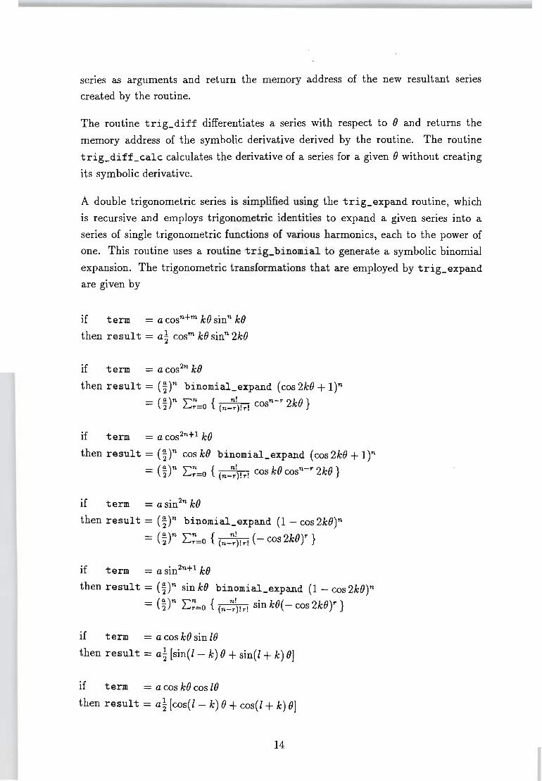
A double trigonometric series is simplified using the trig_expand routine, which
is recursive and employs trigonometric identities to expand a given series into a
series of single trigonometric functions of various harmonics, each to the power of
one. This routine uses a routine trig_binomial to generate a symbolic binomial
expansion. The trigonometric transformations that are employed by trig_expand
are given by
if term = a cosn+m kO sinn kO
then result = a~ cosm kO sinn 2kO
if term = a cos2n kO
then result = (~)n binomial_expand (cos 2kO + l)n _ (Cl)n ~n {n! n-r 2kO} - '2 ~r=O (n-r)!r! cos
if term = a cos2n+1 kO
then result = (~)n cos kO binomial_expand (cos 2kO + 1)n
= (~)n I:~=o { (n-:!)! r! cos kO cosn- r 2kO }
if term = a sin2n k()
then result = (~)n binomial_expand (1 - cos 2k())n
= (Vn I:~=o { (n-:!)! r! ( - cos 2kOY }
if term = a sin 2n+1 k()
then result = (~)n sin kO binomial_expand (1 - cos 2k())n
= (~)n I:~=o { (n-:!)! r! sin kO( - cos 2kOY }
if term = a cos kO sin 10
then result = a! [sin(l- k) 0 + sin(l + k) 0]
if term = a cos kO cos 10
then result = a! [cos(l- k) () + cos(l + k) 0]
14
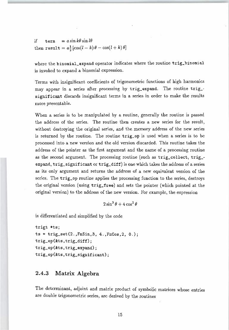
if term = a sin kO sin 10
then result = a~ [cos(l - k) 0 - cos(l + k) 0]
where the binomial_expand operator indicates where the routine trig_binomial
is invoked to expand a binomial expression.
Terms with insignificant coefficients of trigonometric functions of high harmonics
may appear in a series after processing by trig_expand. The routine trig_
significant discards insignificant terms in a series in order to make the results
more presentable.
When a series is to be manipulated by a routine, generally the routine is passed
the address of the series. The routine then creates a new series for the result,
without destroying the original series, and the. memory address of the new series
is returned by the routine. The routine trig_op is used when a series is to be
processed into a new version and the old version discarded. This routine takes the
address of the pointer as the first argument and the name of a processing routine
as the second argument. The processing routine (such as trig_collect, trig_
expand, trig_significant or trig_diff) is one which takes the address of a series
as its only argument and returns the address of a new equivalent version of the
series. The trig_op routine applies the processing function to the series, destroys
the original version (using trig_free) and sets the pointer (which pointed at the
original version) to the address of the new version. For example, the expression
is differentiated and simplified by the code
trigt *ts;
ts = trig_set(2.,FnSin,3, 4.,FnCos,2, 0.);
trig_op(tts,trig_diff);
trig_op(tts,trig_expand);
trig_op(tts,trig_significant);
2.4.3 Matrix Algebra
The determinant, adjoint and matrix product of symbolic matrices whose entries
are double trigonometric series, are derived by the routines
15
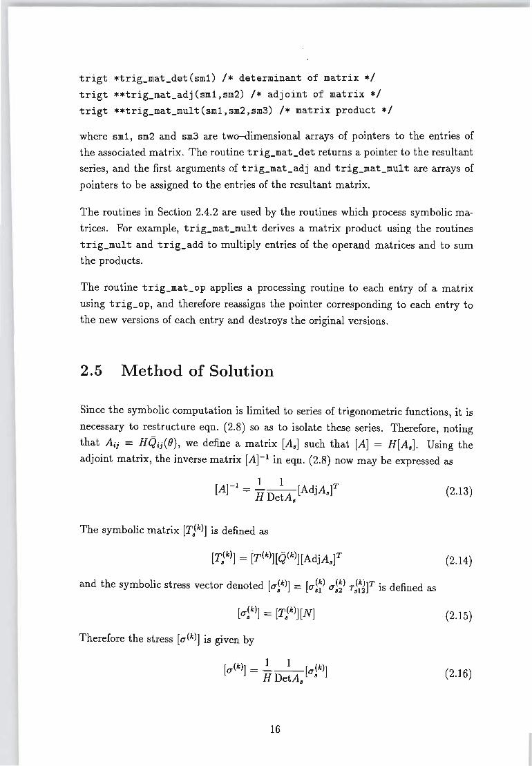
trigt *trig_mat_det(sml) 1* determinant of matrix *1 trigt **trig_mat_adj(sml,sm2) 1* adjoint of matrix *1 trigt **trig_mat_mult(sml,sm2,sm3) 1* matrix product *1
where sml, sm2 and sm3 are two-dimensional arrays of pointers to the entries of
the associated matrix. The routine trig_mat_det returns a pointer to the resultant
series, and the first arguments of trig_mat_adj and trig_mat_mul t are arrays of
pointers to be assigned to the entries of the resultant matrix.
The routines in Section 2.4.2 are used by the routines which process symbolic ma
trices. For example, trig_mat_mul t derives a matrix product using the routines
trig_mul t and trig_add to multiply entries of the operand matrices and to sum
the products.
The routine trig_mat_op applies a processing routine to each entry of a matrix
using trig_op, and therefore reassigns the pointer corresponding to each entry to
the new versions of each entry and destroys the original versions.
2.5 Method of Solution
Since the symbolic computation is limited to series of trigonometric functions, it is
necessary to restructure eqn. (2.8) so as to isolate these series. Therefore, noting
that Aij = HQij(f)), we define a matrix [A6] such that [A] = H[As]. Using the
adjoint matrix, the inverse matrix [A]-l in eqn. (2.8) now may be expressed as
[A]-l = ~ 1 [Ad·A ]T HDetA6 J s
(2.13)
The symbolic matrix [T6(k)] is defined as
(2.14)
and the symbolic stress vector denoted [u!k)] = [u~~) u~;) r::J]T is defined as
(2.15)
Therefore the stress ruCk)] is given by
(2.16)
16
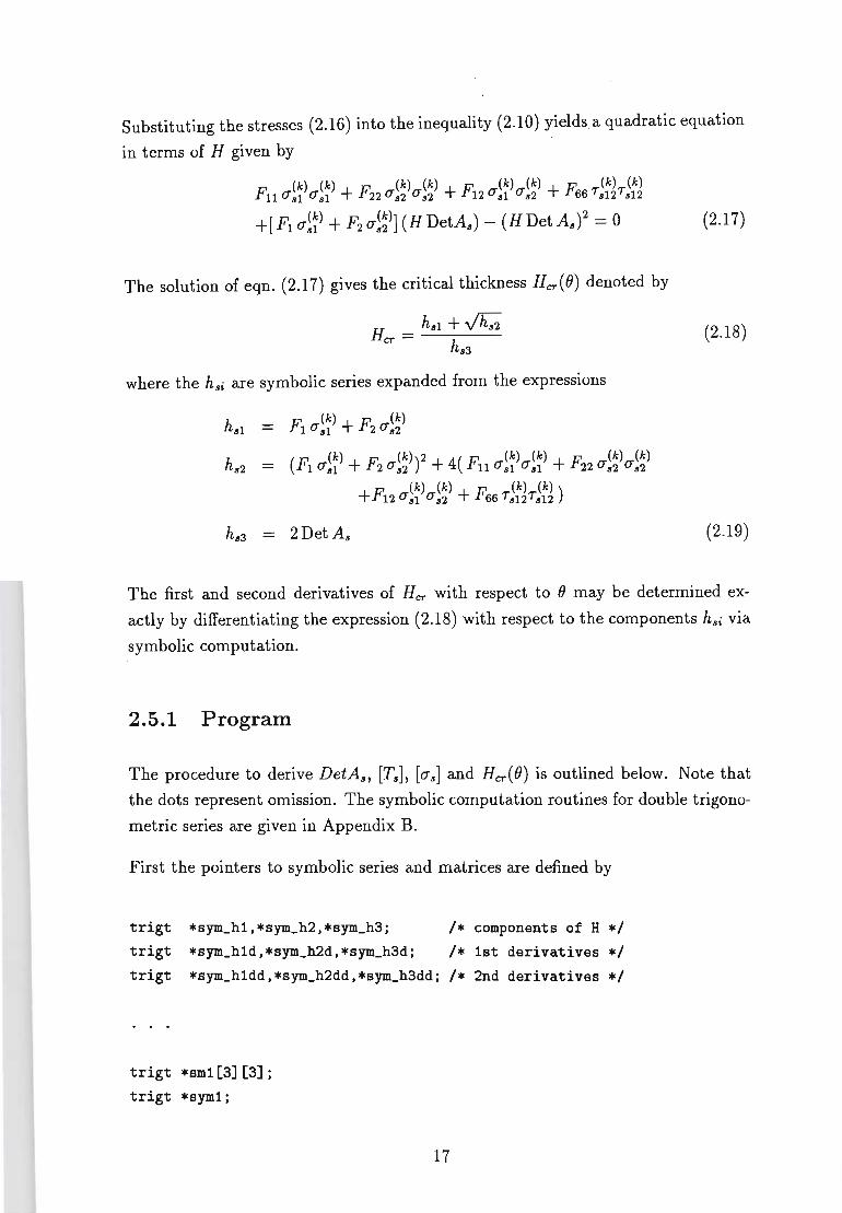
Substituting the stresses (2.16) into the inequality (2.10) yields a quadratic equation
in terms of H given by
(k) (k) (k) (k) F (k) (k) F. (k) (k) Fll 0'31 0'31 + F22 0'152 0'152 + 120'31 0'152 + 66 Td2Ts12
+[ F1 O'~~) + F2 O'~;)] (H DetAs) - (H Det As)2 = 0
The solution of eqn. (2.17) gives the critical thickness Her(fJ) denoted by
Her = hd+~ hs3
where the hsi are symbolic series expanded from the expressions
2Det As
(2.17)
(2.18)
(2.19)
The first and second derivatives of Her with respect to B may be determined ex
actly by differentiating the expression (2.18) with respect to the components hsi via
symbolic computation.
2.5.1 Program
The procedure to derive DetAs, [Ts] , [0'15] and Her(B) is outlined below. Note that
the dots represent omission. The symbolic computation routines for double trigono
metric series are given in Appendix B.
First the pointers to symbolic series and matrices are defined by
trigt
trigt
trigt
*sym_h1,*sym_h2,*sym_h3;
*sym_h1d,*sym_h2d,*sym_h3d;
*sym_h1dd,*sym_h2dd,*sym_h3dd;
trigt *sml[3] [3];
trigt *sym1;
17
1* components of H *1 1* 1st derivatives *1 1* 2nd derivatives *1
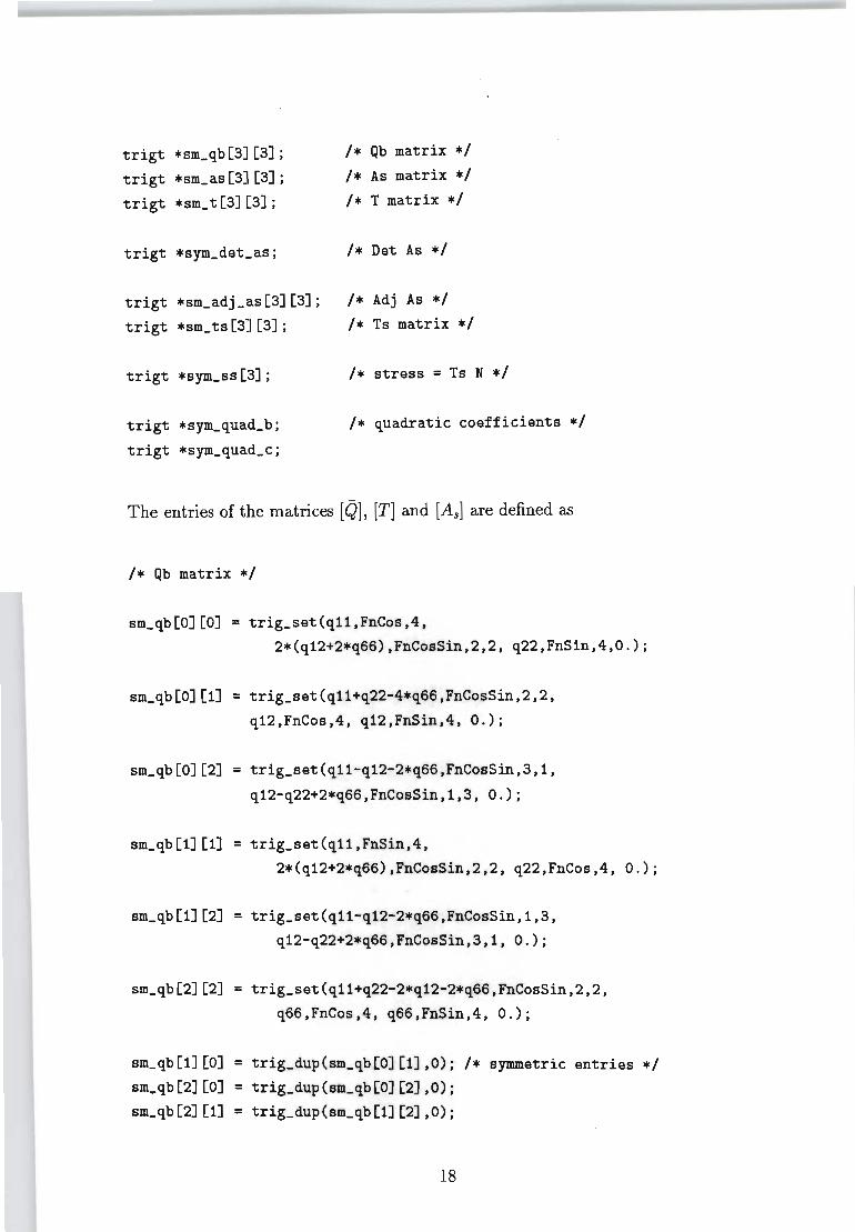
trigt *sm_qb [3] [3] ; 1* Qb matrix *1 trigt *sm_as [3] [3] ; 1* As matrix *1 trigt *sm_ t [3] [3] ; 1* T matrix *1
trigt *sym_det_as; 1* Det As *1
trigt *sm_adj _as [3] [3] ; 1* Adj As *1 trigt *sm_ ts [3] [3] ; 1* Ts matrix *1
trigt *sym_ss [3] ; 1* stress = Ts N *1
trigt *sym_quad_b; 1* quadratic coefficients *1 trigt *sym_quad_c;
The entries of the matrices [Q], [T] and [As] are defined as
1* Qb matrix *1
sm_qb[O] [0] = trig_set(q11,FnCos,4,
2*(q12+2*q66),FnCosSin,2,2, q22,FnSin,4,O.);
sm_qb[O] [1] = trig_set(q11+q22-4*q66,FnCosSin,2,2,
q12,FnCos,4, q12,FnSin,4, 0.) ;
sm_qb[0][2] = trig_set(q11-q12-2*q66,FnCosSin,3,1,
q12-q22+2*q66,FnCosSin,1,3, 0.) ;
sm_qb[1] [1] = trig_set(q11,FnSin,4,
2*(q12+2*q66),FnCosSin,2,2, q22,FnCos,4, 0 . );
sm_qb[1][2] = trig_set(q11-q12-2*q66,FnCosSin,1,3,
q12-q22+2*q66,FnCosSin,3,1, 0.);
sm_qb[2][2] = trig_set(q11+q22-2*q12-2*q66,FnCosSin,2,2,
q66,FnCos,4, q66,FnSin,4, 0.);
sm_qb[1] [0] = trig_dup(sm_qb[O] [1],0); 1* symmetric entries *1 sm_qb[2] [0] = trig_dup(sm_qb[O] [2] ,0);
sm_qb[2] [1] = trig_dup(sm_qb[1] [2] ,0);
18
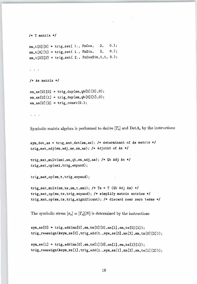
1* T matrix *1
sm_t [0] [0] = trig_set( i., FnCos, 2,
sm_t [0] [1] = trig_set( i., FnSin, 2,
sm_t [0] [2] = trig_set( 2. , FnCosSin,1,1,
1* As matrix *1
sm_as[O][O] = trig_dup(sm_qb[O][O],O);
sm_as[0][1] = trig_dup(sm_qb[0][1],O);
sm_as[O] [2] = trig_const(O.);
0.) ;
0.) ;
0.) ;
Symbolic matrix algebra is performed to derive [Ta] and DetAs by the instructions
sym_det_as = trig_mat_det(sm_as); 1* determinant of As matrix *1 trig_mat_adj(sm_adj_as,sm_as); 1* Adjoint of As *1
trig_mat_mult(sm1,sm_qb,sm_adj_as); 1* Qb Adj As *1 trig_mat_op(sm1,trig_expand);
trig_mat_mult(sm_ts,sm_t,sm1); 1* Ts = T (Qb Adj As) *1 trig_mat_op(sm_ts,trig_expand); 1* simplify matrix entries *1 trig_mat_op(sm_ts,trig_significant); 1* discard near zero terms *1
The symbolic stress [O"s] = [Ts][N] is determined by the instructions
sym_ss[O] = trig_add(nn[O] ,sm_ts[O] [0] ,nn[1] ,sm_ts[O] [1]);
trig_reassign(&sym_ss[0],trig_add(1.,sym_ss[0],nn[2],sm_ts[0][2]));
sym_ss[1] = trig_add(nn[O] ,sm_ts[1] [0] ,nn[1] ,sm_ts[1] [1]);
trig_reassign(&sym_ss[1],trig_add(1.,sym_ss[1],nn[2],sm_ts[1][2]));
19
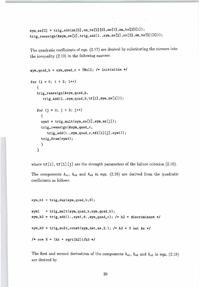
sym_ss [2] = trig_add(nn[O] ,sm_ts [2] [0] ,nn[1] ,sm_ts [2] [1]);
trig_reassign(&sym_ss[2],trig_add(1.,sym_ss[2],nn[2],sm_t5[2][2]));
The quadratic coefficients of eqn. (2.17) are derived by substituting the stresses into
the inequality (2.10) in the following manner.
for (i = 0; i < 3; i++)
{
trig_reassign(&sym_quad_b,
trig_add(i.,sym_quad_b,tf[i],sym_ss[i]));
for (j = 0; j < 3; j++) {
}
symi = trig_mult(sym_ss[i],sym_ss[j]);
trig_reassign(&sym_quad_c,
trig_add(i.,sym_quad_c,tff[i][j],symi));
trig_free(symi );
}
where tf [i], tf [i] [j] are the strength parameters of the failure criterion (2.10).
The components h61, hs2 and hl/3 in eqn. (2.18) are derived from the quadratic
coefficients as follows.
sym1 = trig_mult (sym_quad_b,sym_quad_b);
sym_h2 = trig_add( 1.,symi,4.,sym_quad_c); /* h2 = discriminant */
/* now H = (hi + sqrt(h2))/h3 */
The first and second derivatives of the components hsll hs2 and hs3 in eqn. (2.18)
are derived by
20
sym_hld = trig_diff(sym_hl); 1* first derivatives *1 sym_h2d = trig_diff(sym_h2);
sym_h3d = trig_diff(sym_h3);
sym_hldd = trig_diff(sym_hld); 1* second derivatives *1 sym_h2dd = trig_diff(sym_h2d);
sym_h3dd = trig_diff(sym_h3d);
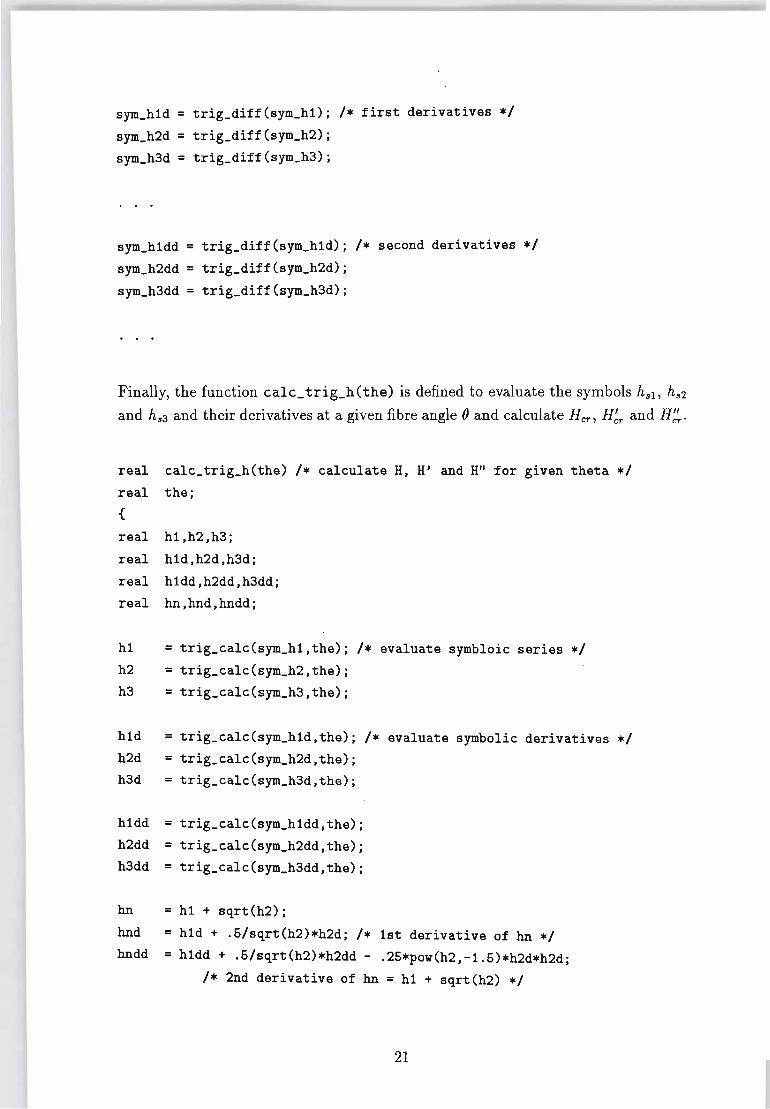
Finally, the function calc_ trig_h (the) is defined to evaluate the symbols hSl' hs2
and hs3 and their derivatives at a given fibre angle () and calculate Her, H~ and H::".
real calc_trig_h(the) 1* calculate H. H' and HI! for given theta *1 real the; {
real hl.h2 .h3;
real hld.h2d.h3d;
real hldd.h2dd.h3dd;
real hn.hnd.hndd;
hi = trig_calc(sym_hl.the); 1* evaluate symbloic series *1 h2 = trig_calc(sym_h2.the);
h3 = trig_calc(sym_h3.the);
hid = trig_calc(sym_hld.the); 1* evaluate symbolic derivatives *1 h2d = trig_calc(sym_h2d,the);
h3d = trig_calc(sym_h3d.the);
hldd = trig_calc(sym_hldd.the);
h2dd = trig_calc(sym_h2dd.the);
h3dd = trig_calc(sym_h3dd.the);
hn = hi + sqrt(h2);
hnd = hid + .5/sqrt(h2)*h2d; 1* 1st derivative of hn *1 hndd = hldd + .5/sqrt(h2)*h2dd - . 25*pow(h2,-1.5)*h2d*h2d;
1* 2nd derivative of hn = hi + sqrt(h2) *1
21
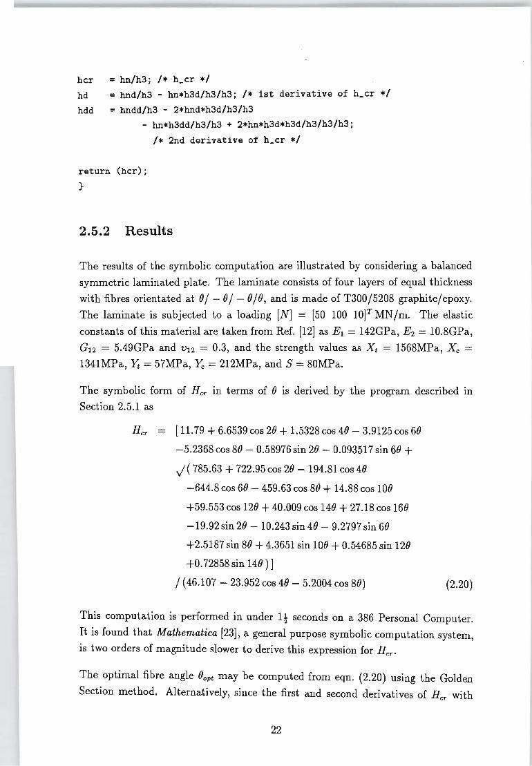
hcr = hn/h3; /* h_cr */ hd = hnd/h3 - hn*h3d/h3/h3; /* 1st derivative of h_cr */
hdd = hndd/h3 - 2*hnd*h3d/h3/h3
- hn*h3dd/h3/h3 + 2*hn*h3d*h3d/h3/h3/h3;
/* 2nd derivative of h_cr */
return (hcr); }
2.5.2 Results
The results of the symbolic computation are illustrated by considering a balanced
symmetric laminated plate. The laminate consists of four layers of equal thickness
with fibres orientated at ()/ - ()/ - ()/(), and is made of T300/5208 graphite/epoxy.
The laminate is subjected to a loading [N] = [50 100 10]T MN/m. The elastic
constants of this material are taken from Ref. [12] as El = 142GPa, E2 = 10.8GPa,
G12 = 5.49GPa and V12 = 0.3, and the strength values as Xt = 1568MPa, Xc = 1341MPa, Yt = 57MPa, Yc = 212MPa, and S = 80MPa.
The symbolic form of Her in terms of () is derived by the program described in
Section 2.5.1 as
Her = [ 11. 79 + 6.6539 cos 2() + 1.5328 cos 4() - 3.9125 cos 6()
-5.2368 cos 8() - 0.58976 sin 2() - 0.093517 sin 6() +
..; ( 785.63 + 722.95 cos 2() - 194.81 cos 4()
-644.8 cos 6() - 459.63 cos 8() + 14.88 cos 10()
+59.553 cos 12() + 40.009 cos 14() + 27.18 cos 16()
-19.92 sin 2() - 10.243 sin 4() - 9.2797 sin 6()
+2.5187 sin 8() + 4.3651 sin 10() + 0.54685 sin 12()
+0.72858 sin 14())]
/ (46.107 - 23.952 cos 4() - 5.2004 cos 8()) (2.20)
This computation is performed in under 1~ seconds on a 386 Personal Computer.
It is found that Mathematica [23], a general purpose symbolic computation system,
is two orders of magnitude slower to derive this expression for Her.
The optimal fibre angle ()opt may be computed from eqn. (2.20) using the Golden
Section method. Alternatively, since the first and second derivatives of Her with
22
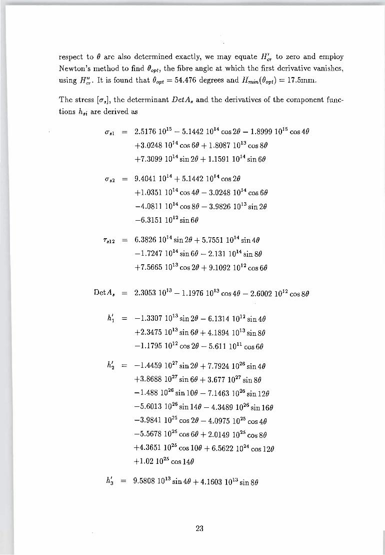
respect to 0 are also determined exactly, we may equate H~ to zero and employ
Newton's method to find Oopt, the fibre angle at which the first derivative vanishes,
using H::". It is found that Oopt = 54.476 degrees and Hmin(Oopt) = 17.5mm.
The stress [0"3]' the determinant DetA3 and the derivatives of the component func
tions h3i are derived as
0"31 = 2.5176 1015 - 5.1442 1014 cos 20 - 1.8999 1015 cos 40
+3.0248 1014 cos 60 + 1.8087 1013 cos 80
+7.3099 1014 sin 20 + 1.15911014 sin60
0"32 9.4041 1014 + 5.1442 1014 cos 20
+ 1.0351 1014 cos 40 - 3.0248 1014 cos 60
-4.0811 1014 cos 80 - 3.9826 1013 sin 20
-6.3151 1012 sin 60
7312 6.3826 1014 sin 20 + 5.75511014 sin 40
-1.7247 1014 sin 60 - 2.1311014 sin80
+ 7.5665 1013 cos 20 + 9.1092 1012 cos 60
DetA3
h' 1
2.3053 1013 - 1.1976 1013 cos 40 - 2.6002 1012 cos 80
-1.3307 1013 sin 20 - 6.13141012 sin 40
+2.34751013 sin60+4.18941013 sin80
-1.1795 1012 cos 20 - 5.611 1011 cos 60
h~ - -1.4459 1027 sin 20 + 7.7924 1026 sin 40
+3.8688 1027 sin 60 + 3.677 1027 sin 80
-1.488 1026 sin 100 - 7.1463 1026 sin 120
-5.6013 1026 sin 140 - 4.3489 1026 sin 160
-3.9841 1025 cos 20 - 4.0975 1025 cos 40
-5.5678 1025 cos 60 + 2.0149 1025 cos 80
+4.3651 1025 cos 100 + 6.5622 1024 cos 120
+ 1.02 1025 cos 140
h; 9.5808 1013 sin40 + 4.1603 1013 sin 80
23
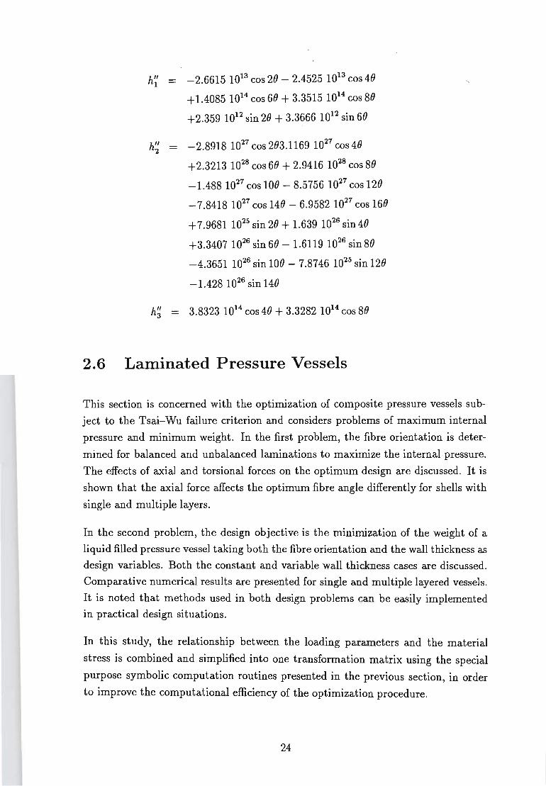
h" _ -2.6615 1013 cos 20 - 2.4525 1013 cos 40 1
+ 1.4085 1014 cos 60 + 3.3515 1014 cos 80
+2.359 1012 sin 20 + 3.3666 1012 sin 60
h" -2.8918 1027 cos 203.1169 1027 cos 40 2
+2.3213 1028 cos 60 + 2.9416 1028 cos 80
-1.488 1027 cos 100 - 8.5756 1027 cos 120
-7.8418 1027 cos 140 - 6.9582 1027 cos 160
+ 7 .9681 1025 sin 20 + 1.639 1026 sin 40
+3.3407 1026 sin 60 - 1.6119 1026 sin 80
-4.36511026 sin 100 - 7.8746 1025 sin 120
-1.428 1026 sin 140
h~ 3.8323 1014 cos 40 + 3.3282 1014 cos 80
2.6 Laminated Pressure Vessels
This section is concerned with the optimization of composite pressure vessels sub
ject to the Tsai-Wu failure criterion and considers problems of maximum internal
pressure and minimum weight. In the first problem, the fibre orientation is deter
mined for balanced and unbalanced laminations to maximize the internal pressure.
The effects of axial and torsional forces on the optimum design are discussed. It is
shown that the axial force affects the optimum fibre angle differently for shells with
single and multiple layers.
In the second problem, the design objective is the minimization of the weight of a
liquid filled pressure vessel taking both the fibre orientation and the wall thickness as
design variables. Both the constant and variable wall thickness cases are discussed.
Comparative numerical results are presented for single and multiple layered vessels.
It is noted that methods used in both design problems can be easily implemented
in practical design situations.
In this study, the relationship between the loading parameters and the material
stress is combined and simplified into one transformation matrix using the special
purpose symbolic computation routines presented in the previous section, in order
to improve the computational efficiency of the optimization procedure.
24
2.6.1 Basic Equations
The pressure vessel is modelled as a symmetrically laminated cylindrical shell of
thickness H, length L and radius R where R refers to the radius of the middle
surface. The shell is constructed of an even number of orthotropic layers of equal
thickness t. The fibre orientation () is defined as the angle between the fibre direction
and the longitudinal axis x. The fibre angles are orientated symmetrically with
respect to the middle surface such that ()k = (_l)k-l() for k ~ n/2 and ()k = (_l)k()
for k ~ n/2 + 1 where k = 1,2, ... , n is the layer number and n is the total number
of layers. It is noted that n = 2 corresponds to a single lamina of thickness H = 2t
and fibre orientation (). The coordinate axes x,</> and z refer to the longitudinal,
circumferential and radial directions respectively, with the origin lying in the middle
surface of the shell.
Due to the symmetry of the lamination, the force resultants in the geometric coor
dinate axes are given by
(2.21 )
where
(2.22)
In eqn. (2.22), Aij are the extensional stiffnesses given by Aij = HQij(()) for i,j =
1,2 and i = j = 6, Ai6 = 2tQi6(()) for unbalanced laminates and Ai6 = 0 for balanced
laminates with i = 1,2. Also in eqn. (2.22), fx, f4> and Ix4> denote the normal and
shear strains. Here Qij(()) is the transformed reduced stiffness component.
The stress-strain equations for the k- th orthotropic layer are given by
[S(k)] = [Q!;)][f]
where [f] = [A]-l[N] from eqn. (2.21), and
denotes the stress vector in the x</> coordinate system.
The stress vector in the material coordinate system, denoted by
25
(2.23)
is obtained from the geometric stress vector [s(k)] via the matrix transformation
(2.24)
where [T(k)] = [T( Ok)] denotes the transformation matrix for the k-th layer. From
eqns. (2.23) and (2.24) it follows that
(2.25)
The design against failure is determined by employing a suitable failure criterion.
In this study, the Tsai-Wu failure criterion (2.10) is used.
The problem formulation and the performance index depend on the nature of the
specific design problem. The problem statement involves maximizing or minimizing
a cost function subject to the strength constraint given by the criterion (2.10). The
optimization procedure is applied to two design problems.
2.6.2 Problem 2.1: Design for Maximum Internal Pressure
We consider a cylindrical pressure vessel with closed ends and subject to an internal
pressure p, axial force F and torque T. The first design problem involves determining
the fibre orientation 0 so as to maximize the internal pressure p for a given laminate
thickness H under the forces F and T such that the optimal design satisfies the
strength criterion (2.10).
Method of solution
The force resultants for this problem are given by
pR F Nc = 2"" - 27rR' NIP = pR, (2.26)
The vector [N] = [Nx NIP NXIPf can be expressed as a sum of two components: one
due to the internal pressure p, and the other due to the external forces F and T , VIZ.
[N] = [N]p p + [N]f (2.27)
where [N]p is the coefficient vector of p, and [N]f incorporates the external forces.
26
From eqns. (2.26) and (2.27), it follows that
(2.28)
Similarly, the strain vector [E] may be expressed as
(2.29)
where [E]p = [A]-I[N]p and [E]f = [A]-I[N]" which follows from eqns. (2.21) and (2.27). Now the stresses in the material coordinates can be computed by in
serting [E] from eqn. (2.29) into eqn. (2.25) which gives
(2.30)
where
(2.31 )
We substitute the stresses from eqn. (2.30) into the strength constraint (2.10) and
obtain a quadratic failure criterion in terms of the internal pressure p as given by
(2.32)
where [u(k)] - [u(k) u(k) r(k)]T and [U(k)]f - [u(k) u(k) r(k)]T p - Ip 2p I2p - If 2f 12f •
Solving the quadratic equation (2.32) for the k-th layer yields the burst pressure
p~) = p~)(O; F, T) corresponding to that layer. The burst pressure of the vessel is given by
P = minp(k) cr k cr (k=1,2, ... ,n) (2.33)
If no positive real solution of eqn. (2.32) exists, then the pressure vessel fails under
external load only, and the solution of the design problem does not exist as there is
no feasible design satisfying the constraint (2.10).
27

Optimal design problem
The design objective is the maximization of the burst pressure PC1" subject to the
failure criterion (2.10). The optimization is carried over the fibre orientation (). The
design problem can be stated as
def ((). F T) _ . (k) Pmax - maxpC1" " - maxmlnpC1" 9 9 k
(2.34)
where PC1"( ()j F, T) is given by eqn. (2.33). The maximum burst pressure pmax is
determined by solving the max-min problem (2.34) which also yields the optimal
fibre orientation ()opt.
The optimization procedure involves the stages of evaluating the burst pressure PC1"
for a given () and iteratively improving ()opt to maximize PC1". Thus the computational
solution consists of successive stages of analysis and optimization until convergence
is obtained. The optimization stage employs the Golden Section method in deter
mining ()opt.
Numerical results for Problem 2.1
The optimization of the laminated pressure vessel is illustrated by considering a
cylindrical shell of mean radius R = 1m and thickness H = O.Olm. The laminate is
made of T300/5208 graphite/epoxy the elastic constants of which are EI = 142GPa,
E2 = 10.8GPa, G12 = 5.49GPa, and V12 = 0.3. The strength values are Xt =
1568MPa, Xc = 1341MPa, Yt = 57MPa, Yc = 212MPa, and S = 80MPa. The
values for the material properties are taken from Ref. [12] .
We first investigate the effect of fibre orientation on the burst pressure PC1" for dif
ferent values of the axial force. Figure 2.1 on Page 36 shows the curves of PC1" versus
() for single-layered, four-layered and six- layered laminates with T = 0 for F = 0
and F = 5MN. It is noted that the results for the four-layered (balanced) laminate
are applicable to balanced laminates with any number of layers. For single-layered
construction, it is observed that ()opt = 0 for F = 0 and ()opt = 90° for F = 5MN.
The burst pressure PC1" is much higher for multilayered laminates with the balanced
case giving the highest burst pressure. The effects of the axial force and torque on
()opt and Pmax are investigated in Table 2.1. For single-layered laminates, ()opt = 0 for
low values of F and jumps to 90° at a certain value of F > 0 which depends on the
amount of torque applied. For multilayered laminates, the fibres align themselves
with the longitudinal axis x as F increases. This result is to be expected on physical
grounds.
28
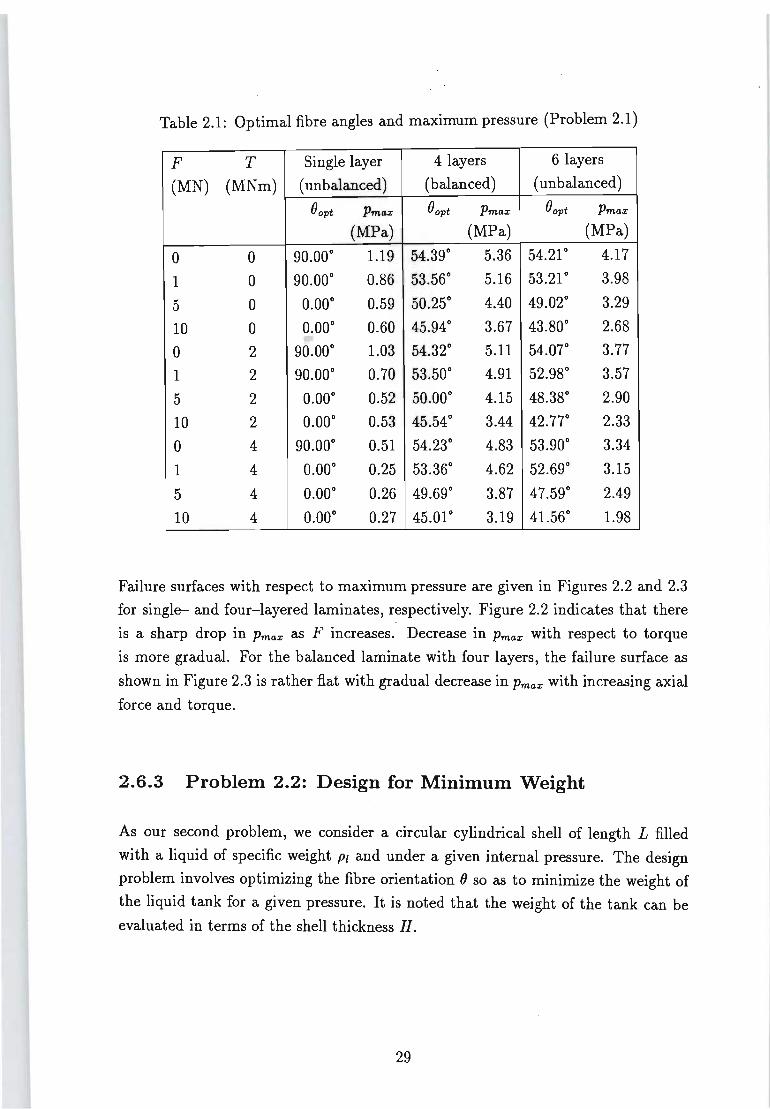
Table 2.1: Optimal fibre angles and maximum pressure · (Problem 2.1)
F T Single layer 4 layers 6 layers
(MN) (MNm) ( unbalanced) (balanced) ( unbalanced)
()opt Pmax ()opt Pmax ()opt Pmax
(MPa) (MPa) (MPa)
0 0 90.00° 1.19 54.39° 5.36 54.21° 4.17
1 0 90.00° 0.86 53.56° 5.16 53.21° 3.98
5 0 0.00° 0.59 50.25° 4.40 49.02° 3.29
10 0 0.00° 0.60 45.94° 3.67 43.80° 2.68
0 2 90.00° 1.03 54.32° 5.11 54.07° 3.77
1 2 90.00° 0.70 53.50° 4.91 52.98° 3.57
5 2 0.00° 0.52 50.00° 4.15 48.38° 2.90
10 2 0.00° 0.53 45.54° 3.44 42.77° 2.33
0 4 90.00° 0.51 54.23° 4.83 53.90° 3.34
1 4 0.00° 0.25 53.36° 4.62 52.69° 3.15
5 4 0.00° 0.26 49.69° 3.87 47.59° 2.49
10 4 0.00° 0.27 45.01° 3.19 41.56° 1.98
Failure surfaces with respect to maximum pressure are given in Figures 2.2 and 2.3
for single- and four-layered laminates, respectively. Figure 2.2 indicates that there
is a sharp drop in Pmax as F increases. Decrease in Pmax with respect to torque
is more gradual. For the balanced laminate with four layers, the failure surface as
shown in Figure 2.3 is rather flat with gradual decrease in Pmax with increasing axial
force and torque.
2.6.3 Problem 2.2: Design for Minimum Weight
As our second problem, we consider a circular cylindrical shell of length L filled
with a liquid of specific weight PI and under a given internal pressure. The design
problem involves optimizing the fibre orientation () so as to minimize the weight of
the liquid tank for a given pressure. It is noted that the weight of the tank can be
evaluated in terms of the shell thickness H.
29
Method of solution
The force resultants for this problem are derived in Refs. [13] and [14]. For a
cylindrical tank with bulkheads attached to the ends of the cylinder, these forces
are
Nz: P;R + ~ cos ¢>(4x2 - L2 - 2R2)
N,p - PcR - PIR2 cos ¢>
-PIRx sin ¢> (2.35)
where Pc 2: PIR is the pressure at the center of the cylinder and x is the longitudinal
axis with the origin located at the mid-point such that -L/2 ~ x ~ L/2.
We note that Aij = Hr/i/Jij(O) where TJij = 1 for i,j = 1,2 and i = j = 6, TJi6 = 2/n
for unbalanced laminates and TJi6 = 0 for balanced laminates with i = 1,2. We define
a matrix [a] such that [a] = H-l[A]. Thus aij = Qij(O) for ij = 11,12,22 and 66, and ai6 = TJi6Qi6(O) for i = 1,2. From eqn. (2.21), it follows that [€] = H-l[a]-l[N] where [N] is defined by eqns. (2.22) and (2.35). Substituting [€] into eqn. (2.25), we
find
(2.36)
where
(2.37)
We substitute the stresses from eqn. (2.36) into the strength constraint (2.10) and
obtain a quadratic failure criterion in terms of the shell thickness H as given by
{F ( (k))2 D (k))2 Po (k))2 F (k) (k)} 11 O"lO + .£'22 0"20 + 66 T120 + 2 120"10 0"20
{ (k) (k)} 2 + FlO"lO + F20"20 H - H = 0 (2.38)
The solution of eqn. (2.38) gives for -any x and ¢> the minimum shell thickness H~)
corresponding to the failure of the k-th layer. From eqn. (2.38), it follows that the
critical thickness Hcr = Hcr(Oj x) at a point x is given by
H = maxH(k) cr ,p,k cr (k = 1, 2, ... ,nj 0 ~ ¢> ~ 271") (2.39)
It is noted that the critical thickness Hcr depends on the location x along the
cylindrical shell as well as the internal pressure Pc and the specific weight PI of the liquid.
30
Optimal design problem
The design objective for the cylindrical liquid tank problem is the minimization of
the shell weight with the thickness subject to the strength condition (2.10). The
weight of the shell is given by
1L/2
W(O) = 27rRpt H(O; x)dx -L/2
(2.40)
where Pt is the specific weight of the fibre composite material used in the construction
of the tank.
Two distinct cases depending on whether the shell thickness is constant or variable
over the length -L/2 ~ x ~ L/2 are considered.
Case I. Constant thickness tank
In this case H = H(O) and the weight is given by
(2.41 )
Since the weight is proportional to the thickness, it is sufficient to minimize H( 0) to
obtain the minimum weight design. Hmin (0) for a given 0 valid for all x is determined
from
Hmin(O) = max Her = max(maxH~») x x "',k (-L/2 ~ x ~ L/2, 0 ~ <P ~ 27r) (2.42)
where H~) is determined from eqn. (2.38).
Case II. Variable thickness tank
In this case H = H(O;x) and the minimum thickness Hmin(O;X) at a point x for a
given 0 is defined by Her in eqn. (2.39). Therefore Hmin(O; x) is determined as the
maximum of H~) given by eqn. (2.39) at every point x producing a variable wall thickness. Thus
H . (0· x) = maxH(k) mm, "',k er (2.43)
Due to symmetry, the thickness distributions are the same for -:-L /2 ~ x ~ 0 and
o ~ x ~ L/2. For this case, the weight is given by eqn. (2.40).
In both cases, the design problem is to determine the optimal fibre orientation Oopt
so as to minimize the weight of the shell, viz.
Wmin = min W(O) o
31
(2.44)
with Hmin obtained from eqn. (2.42) in Case I and from eqn. (2.43) in Case II. In
eqn. (2.44), W(()) is given by eqn. (2.41) for the constant thickness case and by
eqn. (2.40) for the variable thickness case.
The minimum weight problem is solved by determining the minimum thickness
Hmin satisfying the constraint (2.38) from eqn. (2.42) (Case I), or from eqn. (2.43)
(Case II). The weight is minimized over the fibre orientation () by using a one
dimensional numerical optimization scheme, viz. the Golden Section method. Com
putations are continued until convergence is attained for ().
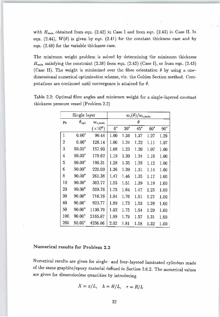
Table 2.2: Optimal fibre angles and minimum weight for a single-layered constant
thickness pressure vessel (Problem 2.2)
Single layer we(())/We,min
Po ()opt We ,min ()
(X 106) 0° 30° 45° 60° 90°
1 0.00° 90.44 1.00 1.36 1.37 1.27 1.29
2 0.00° 128.14 1.00 1.24 1.22 1.11 1.07
3 90.00° 157.93 1.08 1.23 1.20 1.07 1.00
4 90.00° 178.62 1.19 1.30 1.24 1.10 1.00
5 90.00° 199.31 1.28 1.35 1.28 1.12 1.00 .
6 90.00° 220.00 1.36 1.39 1.31 1.14 1.00 8 90.00° 261.38 1.47 1.46 1.35 1.17 1.00 10 90.00° 302.77 1.55 1.51 1.39 1.19 1.00 20 90.00° 509.76 1.75 1.64 1.47 1.25 1.00 30 90.00° 716.76 1.84 1.70 1.51 1.27 1.00 40 90.00° 923.77 1.89 1.73 1.53 1.28 1.00 50 90.00° 1130.79 1.92 1.75 1.54 1.29 1.00 100 90.00° 2165.87 1.99 1.79 1.57 1.31 1.00 200 90.00° 4236.06 2.02 1.81 1.58 1.32 1.00
Numerical results for Problem 2.2
Numerical results are given for single- and four-layered laminated cylinders made
of the same graphite/epoxy material defined in Section 2.6.2. The numerical values
are given for dimensionless quantities by introducing
x = x/ L, h = H/ L, r = R/ L
32
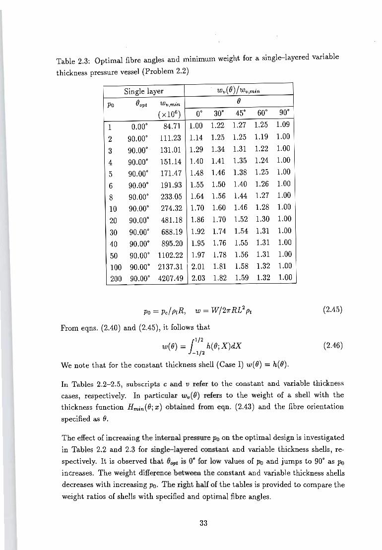
T bl 2 3 Optl·mal fibre angles and minimum weight for a single-layered variable a e .:
thickness pressure vessel (Problem 2.2)
Single layer W1l ( 0) / W 1l,min
Po Oopt W 1I ,min 0
( x106) 0° 30° 45°
1 0.00° 84.71 1.00 1.22 1.27
2 90.00° 111.23 1.14 1.25 1.25
3 90.00° 131.01 1.29 1.34 1.31
4 90.00° 151.14 1.40 1.41 1.35
5 90.00° 171.47 1.48 1.46 1.38
6 90.00° 191.93 1.55 1.50 1.40
8 90.00° 233.05 1.64 1.56 1.44
10 90.00° 274.32 1.70 1.60 1.46
20 90.00° 481.18 1.86 1.70 1.52
30 90.00° 688.19 1.92 1.74 1.54
40 90.00° 895.20 1.95 1.76 1.55
50 90.00° 1102.22 1.97 1.78 1.56
100 90.00° 2137.31 2.01 1.81 1.58 200 90.00° 4207.49 2.03 1.82 1.59
Po = Pc/P1R, w = W/27rRL2 pt
From eqns. (2.40) and (2.45), it follows that
jl/2
w( 0) = h( 0; X)dX -1/2
60°
1.25
1.19
1.22
1.24
1.25
1.26
1.27
1.28
1.30
1.31
1.31
1.31
1.32
1.32
90°
1.09
1.00
1.00
1.00
1.00
1.00
1.00
1.00
1.00
1.00
1.00
1.00
1.00
1.00
We note that for the constant thickness shell (Case I) w(O) = h(O).
(2.45)
(2.46)
In Tables 2.2-2.5, subscripts c and v refer to the constant and variable thickness
cases, respectively. In particular w1l ( 0) refers to the weight of a shell with the
thickness function Hmin(O; x) obtained from eqn. (2.43) and the fibre orientation specified as O.
The effect of increasing the internal pressure Po on the optimal design is investigated
in Tables 2.2 and 2.3 for single-layered constant and variable thickness shells, re
spectively. It is observed that Oopt is 0° for low values of Po and jumps to 90° as Po
increases. The weight difference between the constant and variable thickness shells
decreases with increasing Po. The right half of the tables is provided to compare the
weight ratios of shells with specified and optimal fibre angles.
33
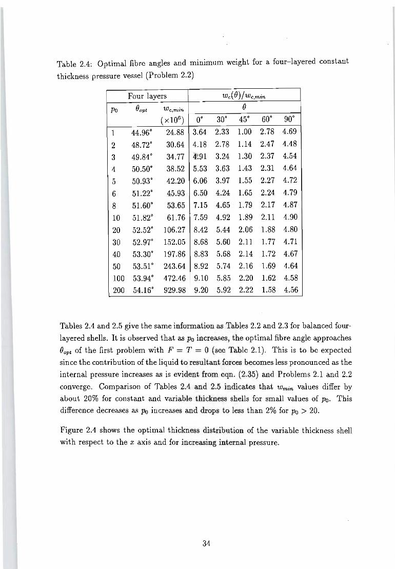
Table 2.4: Optimal fibre angles and minimum weight for a four-layered constant
thickness pressure vessel (Problem 2.2)
Four layers w e( 0) / We ,min
po Oopt We,min 0
( x106) 0° 30° 45° 60° 90°
1 44.96° 24.88 3.64 2.33 1.00 2.78 4.69
2 48.72° 30.64 4.18 2.78 1.14 2.47 4.48
3 49.84° 34.77 4.91 3.24 1.30 2.37 4.54
4 50.50° 38.52 5.53 3.63 1.43 2.31 4.64
5 50.93° 42.20 6.06 3.97 1.55 2.27 4.72
6 51.22° 45.93 6.50 4.24 1.65 2.24 4.79
8 51.60° 53.65 7.15 4.65 1.79 2.17 4.87
10 51.82° 61.76 7.59 4.92 1.89 2.11 4.90
20 52.52° 106.27 8.42 5.44 2.06 1.88 4.80
30 52.97° 152.05 8.68 5.60 2.11 1.77 4.71
40 53.30° 197.86 8.83 5.68 2.14 1.72 4.67
50 53.51 ° 243.64 8.92 5.74 2.16 1.69 4.64
100 53.94° 472.46 9.10 5.85 2.20 1.62 4.58
200 54.16° 929.98 9.20 5.92 2.22 1.58 4.56
Tables 2.4 and 2.5 give the same information as Tables 2.2 and 2.3 for balanced four
layered shells. It is observed that as Po increases, the optimal fibre angle approaches
Oopt of the first problem with F = T = 0 (see Table 2.1). This is to be expected
since the contribution of the liquid to resultant forces becomes less pronounced as the
internal pressure increases as is evident from eqn. (2.35) and Problems 2.1 and 2.2
converge. Comparison of Tables 2.4 and 2.5 indicates that Wmin values differ by
about 20% for constant and variable thickness shells for small values of Po. This
difference decreases as Po increases and drops to less than 2% for Po > 20.
Figure 2.4 shows the optimal thickness distribution of the variable thickness shell
with respect to the x axis and for increasing internal pressure.
34
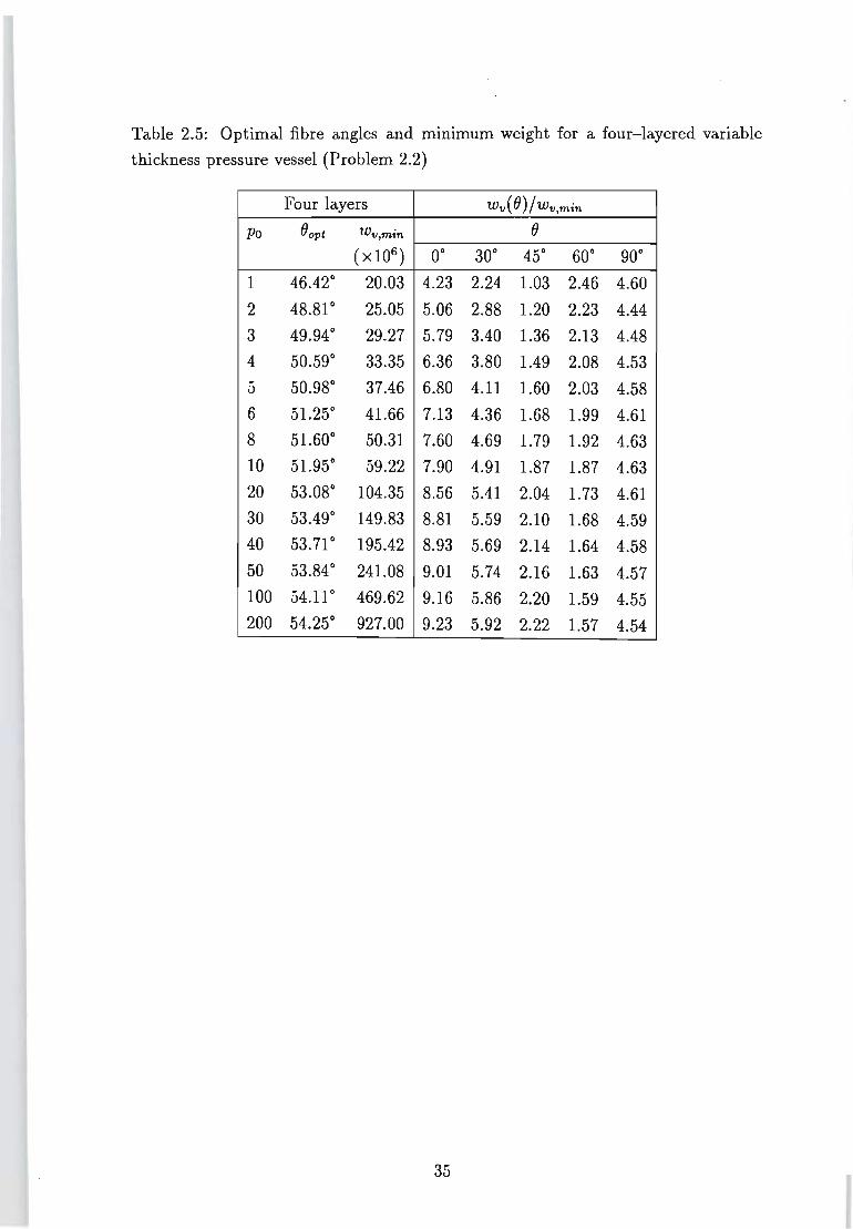
Table 2.5: Optimal fibre angles and minimum weight for a four-layered variable
thickness pressure vessel (Problem 2.2)
Four layers . Wv( ())/Wv,min
po ()opt Wv,min ()
( x106) O· 30· 45· 60· 90·
1 46.42· 20.03 4.23 2.24 1.03 2.46 4.60
2 48.81 • 25.05 5.06 2.88 1.20 2.23 4.44
3 49.94· 29.27 5.79 3.40 1.36 2.13 4.48
4 50.59· 33.35 6.36 3.80 1.49 2.08 4.53
5 50.98· 37.46 6.80 4.11 1.60 2.03 4.58
6 51.25· 41.66 7.13 4.36 1.68 1.99 4.61
8 51.60· 50.31 7.60 4.69 1.79 1.92 4.63
10 51.95· 59.22 7.90 4.91 1.87 1.87 4.63 20 53.08· 104.35 8.56 5.41 2.04 1.73 4.61 30 53.49· 149.83 8.81 5.59 2.10 1.68 4.59 40 53.71· 195.42 8.93 5.69 2.14 1.64 4.58
50 53.84· 241.08 9.01 5.74 2.16 1.63 4.57 100 54.110 469.62 9.16 5.86 2.20 1.59 4.55 200 54.25· 927.00 9.23 5.92 2.22 1.57 4.54
35
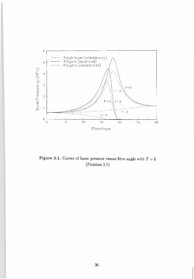
r---.. 0
0.-2 '-../
~ 0.. Q) L
:::J (f) (f) Q) L
0.--+-' (f) L
:::J m
6
Single layer (unbalanced) 5 4 layers ~bOlanc ed)
6 layers unbalanced)
4
3 F= 0
2 , , /
/
\
- --- - -- -\ .-.- -- --\ F=O ----' - ,
F=5 , 0
0 15 30 45 60 75 90
Fibre Angle
Figure 2.1. Curves of burst pressure versus fibre angle with T = 0
(Problem 2.1)
36
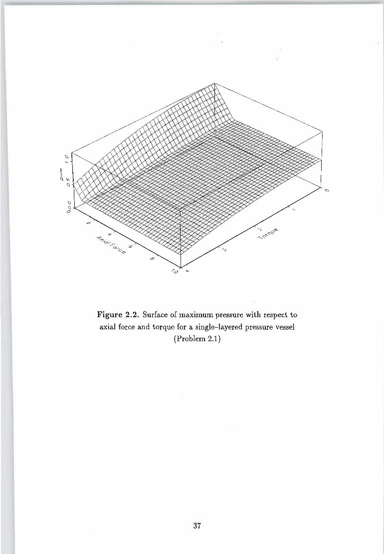
Figure 2.2. Surface of maximum pressure with respect to
axial force and torque for a single-layered pressure vessel
(Problem 2.1)
37
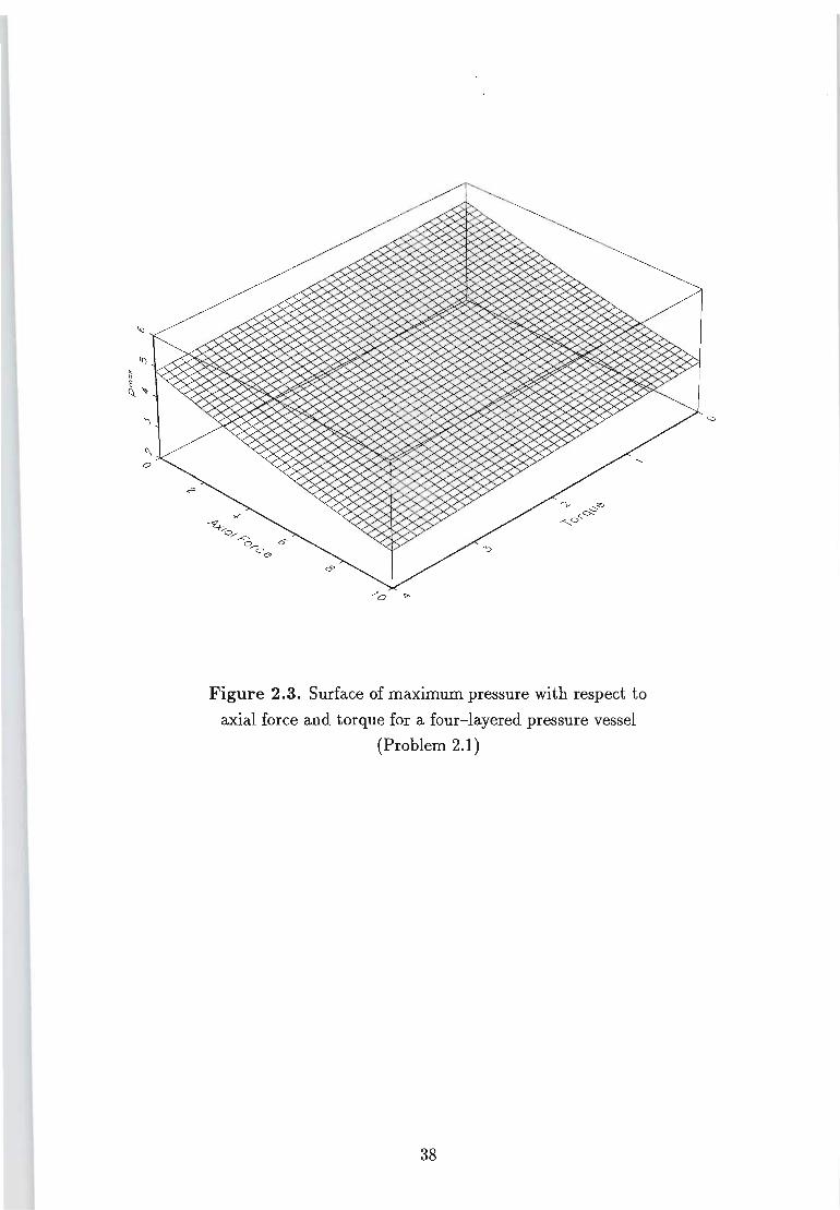
Figure 2.3. Surface of maximum pressure with respect to
axial force and torque for a four-layered pressure vessel
(Problem 2.1)
38
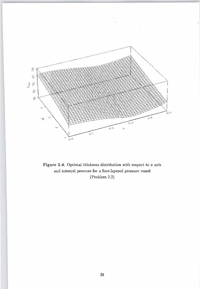
" .~
s:-
0 tfl
0 <t
0 to
O c-J
g ~
~ 0.0
Figure 2.4. Optimal thickness distribution with respect to x axis
and internal pressure for a four-layered pressure vessel
(Problem 2.2)
39
2.7 Conclusions
In design optimization problems requiring symbolic computation, it may be neces
sary to integrate such computations into an iterative solution procedure to improve
the computational efficiency. This is not possible using a closed general purpose
symbolic computation package. In addition, proprietary general purpose symbolic
computation tools often have high overheads in terms of cost, hardware requirements
and processing time. These drawbacks may be overcome by developing special pur
pose symbolic computation software which is tailored according to the requirements
of the specific problem. The development of such software can be realised for a given
problem by noting that, in general, a specific class of functions will be needed in the
solution of a particular problem.
The design problems studied in this Chapter require tedious matrix algebra where
the entries are series of double trigonometric functions of the fibre angle. Special
purpose routines are developed to process such expressions. The routines perform
matrix algebra involving matrices of trigonometric series and simplify the results
using trigonometric identities.
It is found that the special purpose symbolic computation is two orders of magni
tude more efficient than Mathematica. The efficiency of special purpose symbolic
computation arises from its dedication to a specific class .of functions. This feature
is particularly valuable in optimization studies where computational efficiency is
important.
In the laminate example which is considered, the relationship between the loading
parameters and the material stress is combined and simplified into one transfor
mation matrix using symbolic computation. This involves tedious matrix algebra,
where the matrix entries are series of double trigonometric functions of the fibre an
gle. The stress is determined symbolically and substituted into a quadratic failure
criterion from which the critical thickness is obtained as an analytical function of
the fibre angle via symbolic computation. The first and second derivatives of the
critical thickness with respect to fibre angle are determined exactly with the aid of
symbolic differentiation and may be used to determine the optimal fibre angle by
means of an optimization algorithm.
A solution method is presented for the optimal design of symmetrically laminated
cylindrical pressure vessels with balanced and unbalanced stacking sequences on the
basis of a strength failure criterion.
40
Two design problems are solved. In the first problem, a cylindrical pressure vessel
is optimized taking the fibre angle as the design variable to maximize the burst
pressure and the effects of the axial force and torque on the optimal designs are
investigated. In the second problem, a cylindrical vessel filled with a liquid and
subject to an internal pressure is studied. The weight of the shell is minimized
taking the fibre angle and wall thickness as the design variables. Both constant and
variable thickness shells are investigated. It is shown that the results for the second
problem approach those of the first problem as the internal pressure increases.
Numerical results are given for unbalanced (single- and six-layered) and balanced
laminates noting that in the balanced case the number of layers does not affect the
results. It is observed that fibre angles align themselves with the longitudinal axis as
the axial force increases. Variable thickness shells are found to be about 20% more
efficient than the constant thickness shells for low values of the internal pressure
with the difference decreasing as this pressure increases. For single layer pressure
vessels, the optimal fibre angle is found to be either O· or 90· with the switch-over
point depending on the magnitude of the axial force, torque or the internal pressure.
41
Chapter 3
Derivation of a Higher-Order
Theory for Thick Laminated
Plates and Shells
3.1 Introduction
The objective of the present chapter is to derive a nonclassical theory for the accu
rate analysis of thick laminated composite structures. The classical theory is based 1
on the Kirchhoff-Love hypotheses of straight inextensional normals and therefore
neglects the phenomena of transverse shear and normal deformation. The exact
prediction of the stress and strain state of thick laminated structures made of ad
vanced composite materials requires the use of three-dimensional elasticity models.
However, quasi-three-dimensional models based on higher-order theories may accu
rately describe the behaviour of thick structures over some range of applicability and
are considerably less computationally expensive than three-dimensional models.
In this chapter, comprehensive higher-order theory of laminated plates and shells is
presented. This theory considers plates and shells with transversely isotropic layers
of different thicknesses and stiffnesses, and takes into account both transverse shear
and normal deformation.
The theory is based on kinematic hypotheses which are not taken a priori, but
whose form are derived using an iterative technique where the classical Kirchhoff
Love hypotheses are assumed in the first iteration. New variables which have a clear
physical meaning are introduced.
42
The equations of equilibrium and the boundary conditions are determined using
Lagrange's variational principle, and the complete set of boundary conditions is
derived. Various loading and boundary conditions which fully take into account
transverse shear and normal deformation are considered.
The unknown functions in the system of governing differential equations are defined
on an arbitrary reference surface. The stress/strain state of the laminated structure
is determined from the solution at the reference surface and through-the-thickness
distribution functions defined by the theory. The order of the governing equations
is 16 and is independent of the number of layers.
3.2 Literature Survey
The accurate analysis of laminated composite plates and shells is the subject of much
investigation and new higher-order theories have been developed which attempt to
accurately describe the three-dimensional elastic behaviour of laminated plates and
shells. Surveys of these theories may be found in the reviews by Dudchenko et al [25],
Librescu & Reddy [26], Reddy [27], Noor & Burton [28], and in the books of Bolotin
& Novichkov [29], Grigorenko & Vasilenko [30] and Piskunov & Verijenko [31].
The two main approaches for deriving two-dimensional equations of plates and
shells are the analytical method introduced by Reissner [32], Mindlin [33] and
Gol'denveizer [34], and the method of hypotheses.
In the second method, kinematic or static assumptions regarding the variation of
displacements, strains and/or stresses through the thickness are introduced. Two
approaches for the derivation of theories using the method of hypotheses have been
employed, leading to single-layer and discrete-layer theories. In discrete-layer theo
ries, the hypotheses relate to each layer such that the order of the governing differen
tial equations is dependent of the number of layers, whereas in single-layer theories,
the hypotheses relate to displacements, strain and/or stress through the thickness
such that the order of the governing equations is independent of the number of layers.
The generalization ofthe discrete-layer approach is given by Bolotin & Novichkov [29],
Grigorenko & Vasilenko [30] and more recently by Reddy [35]. In principle, discrete
layer theories can model the interlaminar stress more accurately. However, these
theories are computationally expensive as compared to single-layer theories.
43
The single-layer approach was introduced by Ambartsumyan [36] where the classi
cal hypotheses of Kirchoff-Love were used. He then used this approach to derive a
higher-order theory of laminated plates and shells [37]. Examples of other single
layer theories are those of Reissner and Mindlin, first-order theories by Vasilenko
& Savchenko [38] and Grigorenko et al. [39] with both transverse shear and normal
deformation included, and higher-order theories by Stein [40] and Reddy [41]. How
ever in these and other more recent publications mentioned in the reviews [25, 28],
there is no compatibility between the nonlinear kinematic model which considers the
distortion of the normal, and the system of internal forces and moments which are
equivalent to those obtained using the straight line hypothesis. Theories without
these disadvantages have been derived by Piskunov [42] and Rasskazov [43]. The
approach introduced in Ref. [42] has been extended by Piskunov et al. [31, 44] and
Verijenko et al. [45,46, 47] to better represent the interlaminar stresses, include the
direct effect of loading on transverse shear and normal deformation, and increase the
range of applicability of the theory. The higher-order theory derived by Piskunov
et al. in Ref. [44] is presented in this chapter.
A study of the reviews mentioned earlier and some other recent papers [48, 49,
50] reveals that in the design of multilayered structures in which the layers have
significantly different physical characteristics, it is also necessary to consider the
phenomenon of normal deformation.
3.3 Basic Equations
The shell is referenced by a curvilinear coordinate system xlO X2 which is parallel to
the bounding surfaces and the surfaces of contact between the layers. The axes of
the curvilinear orthogonal coordinate Xi = const (i = 1,2) coincide with the principle
lines of curvature. The coordinate z = X3 is normal to the reference surface xlO X2.
The reference surface z = 0 may be positioned arbitrarily in the package of layers.
The layers are assumed to be perfectly bonded, and shells are taken as a geometry
with small curvature relative to their thickness (see Figure 3.1 on Page 59) . The curvatures of the shell are given by kij .
In following derivation, the index k = 1,2 ... n refers to the k-th layer of a laminate
with n layers. The indices i = 1,2 and j = 1,2 refer to the coordinate directions
XI, X2, and the index s has the range s = 1,2,3. A subscripted comma denotes
differentiation with respect to the variables following the comma, and a superscripted
44
( k) refers to the k-th layer.
The loads applied on the external surfaces are p+ = p~(x) and p- = p;(x) (s =
1,2,3) respectively and are functions of the curvilinear orthogonal coordinates x =
{Xl, X2}. The conditions on the external surfaces are
u~~) = -p; (z = ao,k = 1) u~;) = p~ (z = an,k = n)
(3.1)
Since the layers are assumed to be rigidly bonded, the rigidity condition for an
arbitrary surface z = ak-l is given by
U!;-l) (static)
u~k-l) (kinematic)
(3.2)
(3.3)
The components of the deformation of k-th layer (k = 1,2 .. . n) for small bending
are given in Ref. [51] as
2e(~) '3
u(k) + u(k) + 2k . 'u(k) ',3 3,' '3 3
2e~;) (k) + (k) ui,3 u 3,i
(k) e33
(k) U3,3
The displacements of the reference surface (z = 0, k = m) are expressed as
u~m)(x, 0)
u;m) (x, 0) Ui ( x) (i = 1, 2)
w(x)
and the deformations of the reference surface as
", .. '3
1 -(u· · + u ·· ) + k ··w 2 '.3 3.' '3
-w " ,'3
which satisfy the well-known equations [51]
o o
(3.4) (3.5) (3.6)
(3.7)
(3.8)
(3.9)
The generalized Hooke's law for the transversely isotropic k-th layer of the shell [37],
where the surface of isotropy at any point (x, z) is orthogonal to the normal, is given
45
by
(k) [ (k) (k)]J , (k) / E' en - O"n - Vk0"22 Ek - Vk0"33 k
(k) e 22
[ (k) (k)]/ E ,(k) / E' 0"22 - VkO"n k - Vk0"33 k
(k) [(k) (k)] , / E' (k) / E' e33 - - O"n + 0"22 Vk k + 0"33 k
2 (k) e12 O"i~) /Gk
2 (k) e13
(k) /G' 0"13 k
2 (k) e23 O"~;) /G~ (3.10)
where the elastic properties are assumed to be functions of the coordinate Z (ak-l ~
Z ~ ak). Ek(z), Vk(Z) and Gk(z) = E k /[2(1 + Vk)] are the modulus of elasticity,
Poisson's ratio and shear modulus respectively in the plane of isotropy; E~(z) and
Gk(z) are the moduli of elasticity and shear respectively in the transverse direction;
and vHz) is Poisson's ratio, which characterizes the reduction in the plane of isotropy
when tension is applied in the transverse direction.
Classical assumptions are employed to derive basic equations for the derivation of
the nonclassical higher-order theory. If the Kirchoff-Love hypotheses are assumed
to be valid for each layer of the shell, then
2e~;) = 0; e~~) = 0
,..(k) - 0 V33 -
(3.11)
(3.12)
By substituting eqns. (3.10) into the hypotheses (3.11), integrating within the con
ditions (3.2) and using the notation (3.7), we obtain the classical kinematic model
U(k) = U · - W ·z · u3(k) = W
t t ,t, (3.13)
The tangential deformations of the k-th layer are obtained from eqns. (3.13) and (3.8) as
. (k) eij = Cij + K.ijZ (3.14)
where it is noted that C12 = C21, K.12 = K.21 and eW = e~~).
Substituting eqn. (3.14) into eqn. (3.10) and using the static hypothesis (3.12) or
the assumption Ek = 00, the in-plane stresses in the k-th layer are derived as
E Ok [(C22 + Vkcn) + (K22 + VkKll)Z]
Eok(1 - Vk)(CI2 + K12Z)
46
(3.15)
where EOk = Ekl(l - v~).
The transverse stresses cannot be found using Hooke's law because of the hypothe
ses (3.11) and (3.12). Therefore, the transverse stresses are derived using the equa
tions of equilibrium for a shell [51] which for the k-th layer may be expressed as
(k) (k) u · · · + U·33 '1,1 , ,
(k) (k) k . (k) U 33,3 + Ui3 ,i - i1 Ui j
o o
Using eqn. (3.16), the transverse shear stresses are derived as
u~k) = _jZ u~~). dz + A.k ,3 '1,1' alo_l
and using eqn. (3.17), the transverse normal stress are derived as
(3.16)
(3.17)
(3.18)
(3.19)
where A8k( x) are functions of integration which may be derived from the loading
conditions (3.1) and static rigidity condition (3.12).
Substituting the equations for stress (3.15) into the integrals (3.18) and calculating
the functions of integration ~k(X) from the loading and rigidity conditions, the
transverse shear stresses are derived in Ref. [31] as
(k) "f -} +f Ui3 = L..l.W,i lk + Pi 2k + Pi 3k (3.20)
where ~ is the Laplace operator, pi, pt are the external loads and f8k (z) are distri
bution functions given by
where
flk(z)
hk{Z)
f3k(Z)
fk(Z)
f;(z)
B J
BJI
-
f; - fk Bfl I BJ
fk1 BJ-1
AIBJ
l z
EOkdz ao
jZ EOkzdz ao
jan EOkdz ao
jan EOkZdz
ao
47
(3.21 )
(3.22)
The distribution functions f3k (z) enable the loading conditions on the external sur
faces to be satisfied once the reference surface has been positioned in the package of
layers and also take into account the influence of the elastic properties of each layer
on the stress distribution of the components u!;) under external loading.
Substituting the derived transverse shear stress (3.20) into the integral (3.19) and
calculating the functions of integration A3k ( x) from the loading conditions (3.1) and
static rigidity condition (3.12), the transverse normal stress is derived in Ref. [31]
as
(3.23)
where pi, pj are the normal components of the external loads and the functions B~k) are given by
kijCij/sk + kij Kijf9k + (kllc22 - 2k12c12 + k22Cll)fsk
+(kllK 22 - 2k12K12 + k22Kll)f9k (3.24)
The distribution functions in eqns. (3.23) and (3.24) are given by
where
f4k(Z)
fSk(Z)
f6k(Z)
f1k(z)
fSk(Z)
f9k(Z) -
fSk(Z)
f9k(Z) -
FaDj21 D/l - F2k
FaD /31 D /1 - F3k
Fal D/l - 1
Fal D/1
fk - FlkB/ID/l .
f: - FaB /11 D /1
fk - FaB/1 D/l
f: - FaBjll D/l
(3.25)
(3.26)
Substituting eqns. (3.15) for the normal stresses u};) in terms of the deformations
of the reference surface and eqn. (3.23) for the transverse normal stress u~;) into
Hooke's law (3.10), the normal strain is obtained as
(k) _ I ~ I 1 ( _ + _ e33 - 1I0kz W - lIOk Ui,i + E~ pi,d4k + pi,dsk + P3 f6k + pI f1k + Bq) (3.27)
48
The normal strain (3.27) may be expressed as
(3.28)
where B~ = Bu / Ek and we denote the distribution functions of the normal strain as
Q'lk(Z)
Q2k(Z)
Qqk(Z) j9k/ E~ (q = 3 ... 6, 9 = q + 1) (3.29)
Since e~ = u~71, the equation for the normal displacements may be expressed as
(3.30)
The function of integration w(x) + C3k (X) is determined from the conditions (3.11)
and (3.7), ie. u~k)(x,ak_d = u~k-l)(x,ak) and u~m)(x,O) = w(x). Substituting
eqn. (3.28) into (3.30) and integrating, we obtain
where Cu = J; B~dz and we denote the distribution functions of the normal dis
placement through the thickness of the laminated shell as
(q = 1. .. 6) (3.32)
Substituting the equation (3.20) for the the transverse shear stress a!;) into the
expression 2e~;) = aJ;) /G~ from eqn. (3.10), and substituting the equation in (3.31) for the normal displacement u~k) into the expression 2ei3 = u(k3) + u3(k) given in
" ,1
eqn. (3.5), we obtain
where
2e(k) _ u(k) =' a~k)/G' _ u(k) 13 3,1 ,3 k 3,1
- -W,i - Llw,;( C{)lk - C{)k) - Ui,ijC{)2k - P~ijC{)3k - PtijC{)4k
-P3,iC{)Sk - P3,iC{)6k - P"iC{)7k - ptC{)Sk - Cu,i
C{)k(Z) jlk/G~
C{)7k(Z) - - hk/G~
C{)Sk(Z) - - f3k/G~
49
(3.33)
(3.34)
Integrating eqn. (3.33) and satisfying the conditions (3.7) and (3.11), we obtain the
tangential components of the displacement due to transverse shear as
U~k)(X, z) = Ui - W,iZ - D.w,i1/Jlk - Uj,ji1/J2k - Pi,ji1/J3k - PJ,ji1/J4k
-P3-i1/J5k - pji1/J6k - pi1/J7k - pt1/Jsk - Au , ,
where Au = J; Cu,idz and we denote
1% ('Plk - 'Pk)dz
1% 'Pgk dz (9 = 2 ... 8)
(3.35)
(3.36)
The equations derived for e~;), e~ and u1;), u~;) are incompatible with the classical
assumptions and are therefore not relevant to the classical theory. These equations,
however, are important for the derivation of the higher-order theory.
3.4 Higher-Order Theory
The form the kinematic hypotheses of the higher-order theory is taken from eqn. (3.35)
for the displacements u~k) and eqn. (3.31) for the deflection u~k). In particular, the
higher-order theory is based on the kinematic hypotheses
U~k)(X, z)
u~k)(x, z)
Ui - W,iZ - Xg,i1/Jgk (9 = 1 ... 8)
W + Xq'Pqk (q = 1. .. 6)
(3.37)
(3.38)
where Ui(X), w(x) are the displacements of the reference surface; Xl(X), X2(X) are
new functions described below; and we denote
X3(X) = Pi:i; X4(X) = Pti; Xs(x) = P3";
X6(X) = pt; X7,i(X) = pi; XS,i(X) = pt; (3.39)
which are determined from the given loading.
The distribution functions 'Pqk of the deflection through the thickness of the lami
nate are given by eqn. (3.32), and the distribution functions 1/Jgk of the tangential
components of the displacement vector through the thickness of the laminate are given by eqns. (3.36).
The first of the two new unknown functions Xl(X) and X2(X) is termed the shear
function and the second is termed the compression function [56,57]. If Ek =I 00 but
50
vA: = 0 then CP1k = CP2k = .,p2k = 0 and thus X1( x) and X2( x) are also connected with
Poisson's transverse reduction. The interpretation of the functions Xq (x) (q = 1 ... 6)
in eqns. (3.37) and (3.38) is now discussed. Together with the functions cpqk(a)
(q = 1 ... 6) they represent the additional normal deflection of the surface z = a
relative to the deflection of the reference surface. The derivatives Xg,i together with
the functions .,pgk( a) (9 = 1 ... 8) represent the angles of the tangents to the distorted
normal at z = a (in the directions Xi) which are added to the angles of the straight
normals to the displaced reference surface, as illustrated in Figure 3.2. The other
terms involving Xg (9 = 3 ... 8), which are determined from the external loads, take
into account the normal deformation caused by the direct loading.
Substituting the kinematic model given in eqns. (3.37) and (3.38) into the strain
displacement relations given by eqns. (3.4)-(3.6) and using the notation (3.8), the
components of the strain tensor are obtained as
(3.40)
where 9 = 1 ... 8, q = 1 ... 6 and Cij and ""ij are the strains of the reference surface
given by eqn. (3.8); and we denote ""!J) = -Xg,ij and
fJSk(Z) - hk/G~ (3.41 )
It . t d th t (g) - (g) d (g) (g) IS no e a ""n,2 - ""12,1 an ""22,1 = ""12,2.
Using Hooke's law for a transversely isotropic material (3.10), the components of the stress tensor may be determined as
(k) O'n
A (k) A (k) (k) lIken + 12ke22 + A 13ke33
(k) 0'22
A (k) A (k) (k) 12ken + 1Ike 22 + A 13ke33
(k) A [(k) (k)] (k) (3.42) 0'33 - 13k en + e22 + A33ke33 (k) 2G' e(k) 0'12 k 12 (k)
0'13 2G' (k) k e13
(k) 2G' e(k) 0'23 k 23
where
51
A12k D.12k/ D.k
A 13k - D.13k/ D.k
A33k D.33k/ D.k (3.43)
and
D.k (1 + lJk)[1 - lJk - 2(lJ~? Ek/ E~]/ EZE~
D.uk [1 - (lJ~)2 Ek/ E~]/ EkE~
D.12k [lJk + (lJ~)2 Ek/ E~]/ EkE~
D.13k lJ~(1 + lJk)/ EkE~
D.33k (1 - lJ~)/ EZ (3.44)
are the elastic constants for the transversely isotropic k-th layer.
Substituting the components of the strain tensor (3.40) into the stress tensor (3.42)
gIves
(k) O"u
(k) 0"33
AUk(CU + ~uZ + ~W-rPgk + kUXq!.pqk)
+A12k(C22 + ~22Z + ~W-rPgk + k22 Xq!.pqk) + A 13kXq(}qk
A12k(CU + ~uZ + ~~;)-rPgk + kUXq!.pqk)
+AUk (C22 + ~22Z + ~~~-rPgk + k22Xq!.pqk) + A 13kXq(}qk
A13k[cU + C22 + (~u + ~22)Z + (~W + ~W)-rPgk +(ku + k22 )Xq!.pqk] + A33kXq(}qk
2Gk(C12 + ~12Z + ~~~)-rPgk + k12 Xq!.pqk) (k) (
O"i3 - Xt,iJtk
where 9 = 1 ... 8, q = 1 ... 6 and t = 1,2,3.
(3.45)
The above equations define the components of the displacement vector and the
stress and strain tensors at an arbitrary point in the k-th layer. The model equa
tions include: the system of independent unknown functions of the reference surface
Ui, W, Xp (i,p = 1,2); the known functions Xg (g = 3 ... 8) which are determined from
the given loads p- , p+ on the external surfaces; and the system of known functions
of the normal coordinate z, incorporating the laws governing the variation of the
components of the displacement vector and of the stress and strain tensors through
the thickness of the package of layers. Clearly, the describing equations are not
dependent on the thicknesses, stiffnesses and other properties of the layers. More
over, the equations of this model may consider layers with elastic characteristics
that are constant or variable. Thus the model is comprehensive with respect to the
configuration of the package of layers.
52
3.5 Equilibrium & Boundary Conditions
The equations of equilibrium and the boundary conditions are determined using the
Lagrange variational principle as follows:
OU = orr + J J fv {e1~) + ~~ [O"i~) + O"~~)] - ~k 0"1;)} 00"1;) dV - oH = 0 (3.46)
where orr is the variation of the potential energy of deformation, and oH is the
variation of the work of the external forces. Using the components of the strain
tensor in eqns. (3.40), we derive
orr = J fs{l:n[O"~k)o(cij + K,ijZ + K,~;)1jJgk + kijXq<{)q)
+O"};)O(Xt,i,Btk) + 0"1;)0(XqQqk)]dz }dS
where i,j = 1,2, t = 1,7,8, q = 1 ... 6 and 9 = 1 ... 8.
(3.47)
Using notation similar to that of classical theory, the forces and moments are ex
pressed as integrals of the stresses, viz.
N; . = jan O"~~) dz . '1 '1' ao
M·· = jan O"~~) Z dz . '1 '1 ,
ao (3.48)
Higher-order forces and moments which describe the influence of transverse shear
and normal deformation are denoted
N~1!) = jan O"~~)(,., k dz . '1 '1 TP ,
ao
Q(1) = l an O"~k),B kdz . , ,3 I ,
ao
where p = 1,2.
Eqn. (3.46) may be expressed using these forces and moments as
orr = J fs[NijOUi,j + Nijkijow - MijoW,ij - Mi1)oxP,ij
+Ni1)kij oXp + Q!I)OXl,i + Q~p)OXp] dS
where p = 1,2.
(3.49)
(3.50)
The variation of the work of the external loads consists of the variation of the load
HI which is applied to the bounding surfaces and that of the boundary forces H2
•
Therefore
J is[p-; OU~I) + p; ou~n)]dS
l {l:n
[O"i~ ou~k) + O"i~) ou~k) + 0"17) oufk)]dz }dL
53
(3.51 )
(3.52)
where s = 1,2,3; hand 1 are the normal and tangent to the boundary L of the shell;
ul~, ul;) and ul7) are components of the stress tensor at an arbitrary point in the
k-th layer on the edge L of the shell.
Using the hypotheses (3.37) and (3.38), the variation of the work of the given loading
is expressed as
J !s(PiOUi + P30W + pr)OXp) dS
-i (Ph OW + p~)OXp) dL (3.53)
where the summation index P = 1,2, we denote h = i and the generalized loads are
given by
- + + Pi - Pi Pi
-+ ++-++ P3 aOPi,i anPi,i P3 P3
pr) tPp1(aO)p~i + tPpn(an)pti + <pp1(aO)P3 + <ppn(an)p3
Ph - aop"i: + anpt
p~) tPp1(aO)p"i: + tPpn(an)pt (3.54)
Equating the variation of given functions to zero, we may express eqn. (3.52) as
oH2 = i {N~hOUh + Nh10Ul - Mhhow,h .- Mzlp)oxp,h
+(Mh1.1 + Qh)OW + [MZf~) + Q~(p)]oXp}dL -[Mh1.10W + MZ1(P)Oxp]f~ (3.55)
where an asterisk denotes forces acting on the boundary of the shell, and we denote
(3.56)
The equations of equilibrium may now be obtained as
N. ... +p' - 0 '3.3 , -
Mij•ij - kij Nij + P3 = 0
M (l) Q(l) Q(l) (1) (1) .... + .. - - k ·· N .. +p - 0 '3.'3 '.' 3 '3 '3 3-
M~?~. - Q(2) _ k .. N~?) + p(2) - 0 '3.'3 3 '3 '3 3- (3.57)
and the boundary conditions are given by
54
(Nhl - Nhl ) OUI = 0
(Mhh,h + 2Mhl,1 + Ph - R~) OW = 0
(Mhh - Mhh)OW,h = 0
(Mn) - M~11») OX1,h = 0
(M~~ - M~12») OX2,h = 0
(M(1) + 2M(1) + Q(1) + p(1) _ R*(1») OX1 = 0 hh,h hl,1 h h h
(M(2) + 2M(2) + p(2) - R*(2») OX2 - 0 hh,h hl,1 h h -
where we denote the generalized reactions
R~ = Q~ + Mhl,l; R~(p) = Q~(p) + M~,(,~)
(3.58)
(3.59)
Modelling different constraints on the boundary of the shell is now considered on
the basis of these boundary conditions. The first group of constraints corresponds
to the four degrees of freedom Uh, UI, W, W,h. These external boundary conditions
are modelling constraints belonging to the boundary of the two-dimensional region
of the reference surface of the shell (z = 0), and determine in general the type of
support for the shell. The second group of constraints given by the conditions (3.58)
models the constraints on the boundary through the thickness of the shell as shown
in Figure' 3.3. This group of internal boundary conditions concerns the modelling of
transverse shear and normal deformation at the edges of the shell. The laminate is
modelled more accurately when both types of boundary conditions are considered.
Substituting the components of the stress tensor (3.45) into the integrals (3.48)
and (3.49) yields the equations of elasticity, viz. the equations for the generalized
forces and moments. Thus the in-plane forces may be expressed as
Nu = Bcu + BC22 + BoKu + BoK22
+BgK~'i) + BqKW + (kuCq + k22 Cq + Hq)Xq
N22 ~ Nu
N12 - (B - B)C12 + (Bo - BO)K12 + (Bg - Bg)K~~,>
+k12 (Cq - Cq)Xq (3.60)
where q = 1 ... 6 and 9 = 1 ... 8. The bending and twisting moments may be expressed as
Mu - Bocu + Boc22 + DooKu + DOOK22
+DogKW + DogK~~) + (kuCoq + k22 COq + Hoq)Xq
M22 ~ Mu
55
the higher-order forces and moments as
N (p) 11
N (p ) 22
~ N(p) ~ 11
N (p ) 12 (Tp - Tp)C12 + (TpO - TpO)~12
+(Tpq - Tpq)~W + kl2(Lpq - Lpq)Xq
M (p) 11
- - (g) BpC11 + BpC22 + DpO~11 + DpO~22 + Dp9~11
- (g) -) +Dp9~22 + (k11Cpq + k22 Cpq + Hpq Xq
M (p) ~ M(p) 22 ~ 11
Ml~) (Bp - .8p )CI2 + (DpO - DpO)~12 - (g) -
+(Dpg - Dp9)~12 + kl2(Cpq - Cpq)Xq
and the shear forces as
Qi DtXt,i
Q,(.I) D tXt,i
Q~) - PP(C11 + C22) + PpO(~11 + ~22) +Ppg(~W + ~W) + Rpg(k11 + k22 )Xq + f4qXq
where p = 1,2, t = 1,7,8, q = 1 ... 6 and 9 = 1 ... 8.
(3.61 )
(3.62)
(3.63)
The equations for the generalized forces and moments include the integrated stiff
nesses of heterogeneous shells given by
56
B = ran Allkdz Jao
Bo = I:on A 1lkzdz
Bg = I:on Allk-rPgkdz
Cq = I:on Allk<,Oqkdz
Hq = I:on A13kaqkdz
Doo = I:on A 12kZ2dz
Dog = I:on A12k-rPgkZdz
COg = I:on A 12k<,OqkZdz
DpO = Dop
Dpg = I:on Allk-rPpk-rPgkdz
Cpq = I:on A 1lk-rPpk<,Oqkdz
Hpq = I:on A13k-rPpkaqkdz
Tp = I:on A12k<,Opkdz
Tpo = I:on A12k<,OpkZdz
Tpg = I:on A 12k<,Opk-rPgkdz
Lpg = I:on A12k<,Opk<,Ogkdz
Dt = I:on ftk dz
Pp = I:on A13kapkdz
Ppg = I:on A13kapk-rPgkdz
14g = I:on A33kapkagkdz
13 = ran A12kdz Jao
130 = I:on A12kZdz
Bg = I:on A 12k-rPgkdz
Cq = I:on A12k<,Oqkdz
Doo = I:on AllkZ2dz
Dog = I:on Allk-rPgkZdz
COg = I:on Allk<,OqkZdz
Hoq = I:; A13kaqkZdz
DpO = Dop
Dpg = I:on A12k-rPpk-rPgkdz
Cpq = I:on A12k-rPpk<,Oqkdz
Tp = I:on Allk<,Opkdz
T pO = I:on Allk<,OpkZdz
Tpg = I:; Allk<,Opk-rPgkdz
Lpg = I:on Allk<,Opk<,Ogkdz
Ppg = I:on A13k<,Opkagkdz
Dt = I~n ftk/3lkdz
Ppo = I:on A13kapkzdz
Rpg = I:on A13kapk<,Ogkdz
(3.64)
The system of governing differential'equations for heterogeneous composite shells is
expressed in matrix form as
[D]{V} = [Dp]{P} (3.65)
where [D] is the matrix of differential operators on the vector of unknown functions
(3.66)
and [Dp] is the matrix of differential operators on the vector of given loads
(3.67)
The integrated stiffnesses, all of which are given in eqn. (3.64), appear in the matrices
[D] and [Dp], in particular, as coefficients of differential operators.
The order of the general system of differential equations (3.65) is sixteen. Therefore
eight boundary conditions have to be satisfied on each edge of the shelL
One of the advantages of this higher-order theory is that the equations for the
tangential components of the displacement vector and the stress and strain tensors
57

consist of similar terms which separately take into account the states of pure bend
ing, transverse shear and normal deformation. This enables efficient analytical and
numerical application of this theory using an independent but analogous approxima
tion of the components of the displacement vector which belong to these states. It
also allows the experience gained in using analytical and numerical methods in sim
ilar applications but on the basis of classical theory to be extended to a nonclassical
approach based on higher-order theory.
58
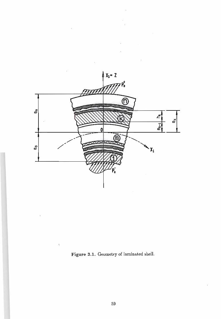
c CD
o CD
Xa= Z
Figure 3.1. Geometry of laminated shell.
59
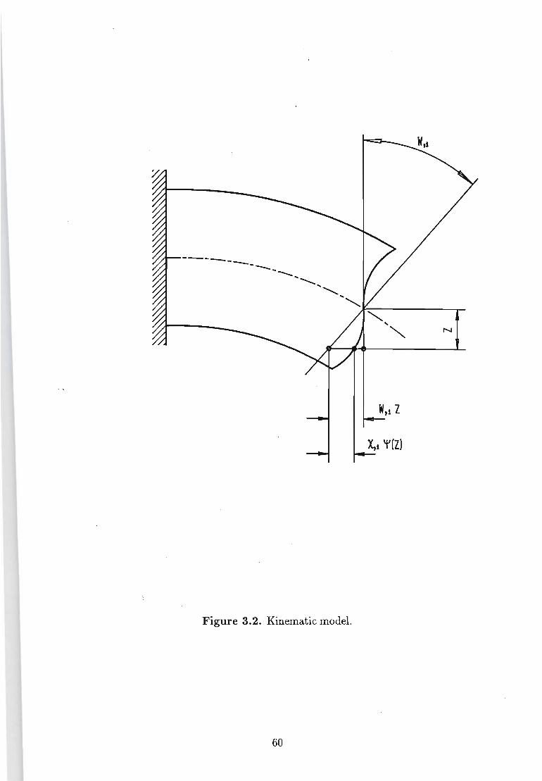
N
W,1 Z
X,1 'f'(Z)
Figure 3.2. Kinematic model.
60
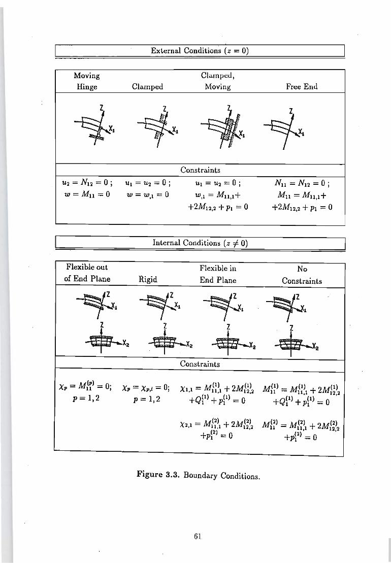
External Condi tions (z - 0)
Moving Cla.mpeu, Hinge Clamped Moving Free End
~. ~. ~
~l~x. ~~ Constraints
'U2 = N12 = 0 ; 'Ul = 'U2 = 0 ; Ul = U2 = 0 ; Nu - N12 - 0 ; ·w = Mu = 0 w = WI = 0 , W,l = M ll,l1- MIl = M ll ,l1-
1-2M12 ,2 1- PI = 0 1-2M12,21- PI = 0
Internal Conditions (z =f. 0)
Flexible out Flexible in No of End Plane Rigid End Plane Constraints
¥. ~. ~. ~ ..
Z Z Z Z -+-x. -+-x. ~. ~. Constraints
X - M(p) - O· XI' = XI',' = OJ M(l) 2M(1) M(l) - M(l) 1- 2M(1) 1'- 11 - , XI,l = 11,1 1- 12,2 11 - 11,1 12,2
P = 1,2 P= 1,2 1-Q~l) 1- p~l) = 0 1-Q~l) 1- p1l) = 0
M(2) M(2) M(2) - M(2) 1- 2M(2) X2,1 = 11,1 1- 2 12,2 U - 11,1 12,2 1-pi2) = 0 1-pi2
) = 0
Figure 3.3. Boundary Conditions.
61
3.6 Conclusions
A higher-order theory of laminated shells and plates subject to both transverse shear
and normal deformation is derived. The proposed theory is capable of analysing
thick plates and shells with an arbitrary number of transversely isotropic layers
which have significantly different elastic properties. Moreover, the layers may be
constructed of materials which have low transverse rigidity.
The kinematic hypotheses of the higher-order theory are not taken a priori but are
formulated using an iterative technique where the classical Kirchhoff-Love hypothe
ses are assumed in the first iteration. Moreover, the new variables introduced by
the theory have a clear physical meaning.
The unknown functions in the system of governing differential equations are defined
on an arbitrary reference surface in the package of layers, and the order of the
governing equations is independent of the number of layers.
Various loading and boundary conditions are considered which enable transverse
shear and normal deformation to be fully taken into account, and the complete set
of boundary conditions is derived.
62
Chapter 4
Implementation of the
Higher-Order Theory using
Symbolic Computation
4.1 Introduction
The objective of this chapter is to implement the higher-order theory presented in
Chapter 3 for the numerical analysis of plates and shells based on an analytical
solution.
The distribution functions and integrated stiffness constants of the higher-order
theory involve multiple piecewise integrals through the thickness of the laminate,
and in the general case these integrals cannot be expressed in an exact form for
direct implementation into a computer program. Therefore symbolic computation
is employed for the implementation of the higher-order theory.
The general purpose Mathematica symbolic computation system is used to derive
the distribution functions, calculate the integrated stiffness constants, solve the
system of governing differential equations analytically and finally to evaluate the
stress/strain state for a given laminate.
In order to improve the computational efficiency of the analysis, special purpose
symbolic computation routines are developed in the C programming language as
an alternative to using a general purpose symbolic computation system such as
M athematica.
63
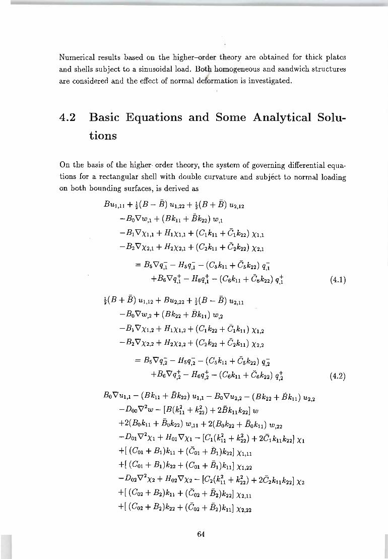
Numerical results based on the higher-order theory are obtained for thick plates
and shells subject to a sinusoidal load. Both homogeneous and sandwich structures
are considered and the effect of normal deformation is investigated.
4.2 Basic Equations and Some Analytical Solu
tions
On the basis of the higher-order theory, the system of governing differential equa
tions for a rectangular shell with double curvature and subject to normal loading
on both bounding surfaces, is derived as
BUl,U + HB - B) Ul,22 + HB + B) U2,12
-BO\1W,l + (Bku + Bk22 ) W,l
-Bl \1Xl,l + HlXl,l + (ClkU + Clk22 ) Xl,l
-B2 \1X2,1 + H2X2,1 + (C2kU + C2k22 ) X2,1
= Bs \1 q~ - Hsq~ - (Csku + CS k22) q~
+Bs\1q1- Hsq1- (Csku + CS k22) q1
HB + B) Ul,12 + BU2,22 + HB - B) U2,U
-Bo\1w,2 + (Bk22 + Bku) W,2
-Bl \1Xl,2 + Hl Xl,2 + (Cl k22 + ClkU) Xl,2
-B2 \1X2,2 + H2X2,2 + (C2k22 + C2kU) X2,2
= Bs \1 q~ - Hsq~ - (Csku + CS k22) q~ + + -+Bs\1q,2 - Hsq,2 - (Csku + CSk22) q~
Bo \1Ul,l - (Bku + Bk22 ) Ul,l - Bo \1U2,2 - (Bk22 + Bku) U2,2
-Doo \12w - [B(k:l + ki2) + 2Bkuk22] w
+2(Boku + Bok22) W,U + 2(Bok22 + Boku) W,22
-DOl \12Xl + HOI \1Xl - [Cl(k:l + ki2) + 2Cl ku k22] Xl
+[ (COl + Bl)ku + (COl + Bl )k22] Xl,U
+[ (COl + Bdk22 + (COl + Bl)ku ] Xl,22
-D02 \12
X2 + H02 \1X2 - [C2(k:l + k~2) + 2C2kUk22] X2
+[ (C02 + B2)ku + (C02 + B2)k22] X2,U
+[ (C02 + B2)k22 + (C02 + B2)ku] X2,22
64
( 4.1)
(4.2)

= DOS'\l2q- - Hos'\lq-
-[CS(k;l + ki2) + 2Csku k22 - 1] q-
-[ (Cos + Bs)ku + (Cos + Bs)k22] q~l
-[ (Cos + Bs)k22 + (Cos + Bs)ku ] q~2
Bl '\lUl,l - HlUl,l - (ClkU + Cl k22 ) Ul,l
+Bl '\lu2,2 - HlU2,2 - (Clk22 + ClkU) U2,2
+DOl '\l2w - HOI '\lw - [Cl(k;l + ki2) + 2ClkUkd w
+[ (COl + Bdku + (COl + Bdk22] W,U
+[ (COl + Bl)k22 + (COl + Bl)ku ] W,22
-Du '\l2Xl + (2Hu + Dd'\lXl
-[Ru + Lu(k;l + ki2) + 2kuk22Lu + 2Pu(ku + k22 )] Xl
+2( CukU + CUk22) Xl,U
+2(Cu k22 + CukU) Xl,22 2 -
-D12'\l X2 + (2H12 + P12 )'\lX2 - 2 2 -
-[R12 + L12(kU + k22 ) + 2kuk22L12
+(P12 + R12)(ku + k22] X2
+[ (C12 + T12)ku + (C12 + T12 )k22] X2,U
+[ (C12 + T12)k22 + (C12 + T12)ku] X2,22 .
= DIS '\l2q- - (HIS + PlS)'\l q-
+[RlS - !;?u(ao) + (PIS + RlS)(ku + k22 ) 22-+LlS(kU + k22 ) + 2kuk22LlS] q-
-[ (CIS + TlS)ku + (CIS + TlS )k22] q~l
-[ (CIS + TlS )k22 + (CIS + TlS)ku ] q22 , 2 + - + +D16'\l q - (H16 + PI6)'\lq
+[R16 - !;?In(an) + (P16 + R16)(ku + k22 ) 2 2 - + +L16(ku + k22 ) + 2kuk22L16] q
-[ (C16 + T16)ku + (C16 + T16 )k22] q!l ,
-[ (C16 + T16)k22 + (C16 + T16)ku ] q12 ,
B2'\lUl,1 - H21J},1 - (C2kU + C2k22 ) Ul,l
+B2'\lU2,2 - H2U2,2 - (C2k22 + C2kU) U2,2 2 [2 2 -+D02'\l w - H02'\lW - C2(kU + k22 ) + 2C2kUk22] w
65
(4.3)
(4.4)
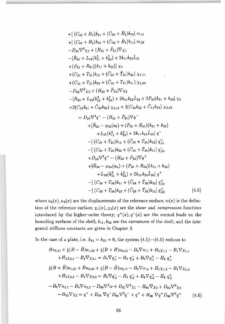
+[ (C02 + B2)kn + (002 + B2)k22] W,n
+[ (C02 + B2)k22 + (002 + B2)kn ] W,22
-D2l V 2Xl + (H2l + P2l)VXl
-[R2l + L2l (k;1 + ki2) + 2knk22£2l
+(P2l + R2l )(kn + k22 )] Xl
+(C2l + T2l)kn + (021 + T21 )k22 ) Xl,n
+(C2l + T21)k22 + (021 + T21)kn) Xl,22
-D22V 2X2 + (H22 + P22 )VX2
-[R22 + L22(kil + k~2) + 2knk22£22 + 2P22 (kn + k22] X2
+2(C22kn + 022k22) X2,n + 2(C22 k22 + Onk22) X2,22
= D2SV2q- - (H2S + P2S )Vq-
+[R2S - 'P2l(aO) + (P2S + R2s)(kn + k22 ) 22-+L2s(kn + k22 ) + 2knk22L2S] q-
-[ (C2S + T2s)kn + (025 + T2S )k22] q;1l
-[ (C2S + T2S)k22 + (025 + T2S)kn ] q~2
+D26V 2q+ - (H26 + P26 )Vq+
+[R26 - 'P2n(an) + (P26 + R26)(kn + k22 ) 2 2 - + +L26(kn + k22 ) + 2knk22L26] q
- - + -[ (C26 + T26)kn + (C26 + T26)k22] q,n
- - + -[ (C26 + T26)k22 + (C26 + T26)kn ] q22 , (4.5)
where Ul (x), U2 (x) are the displacements of the reference surface; w( x) is the deflec
tion of the reference surface; Xl(X), X2(X) are the shear and compression functions
introduced by the higher-order theory; q+(x), q-(x) are the normal loads on the
bounding surfaces of the shell; kn, k22 are the curvatures of the shell; and the inte
grated stiffness constants are given in Chapter 3.
In the case of a plate, i.e. kn = k22 = 0, the system (4.1)-(4.5) reduces to
BUl,n + HB - B)Ul,22 + HB + B)U2,12 - Bo VW,l + HlXl,l - Bl VXl,l
+H2X2,1 - B2VX2,1 = BsVq;1 - Hs q;1 + B6V q1- H6 q1
HB + B)Ul,2l + BU2,22 + HB - B)U2,n - Bo VW,l + H1Xl,2 - Bl VXl,2
+H2X2,2 - B2VX2,2 = BsVq~ - Hs q~ + B6Vq~ - H6 q~
-Bo VUI,1 - Bo VU2,2 - Doo V 2w + DOl V 2Xl - HOI VXl + D02 V 2X2
-H02VX2 = q- + Hos Vq- DosV2q- + q+ + Hoo Vq+ DooV2q+ (4.6)
66
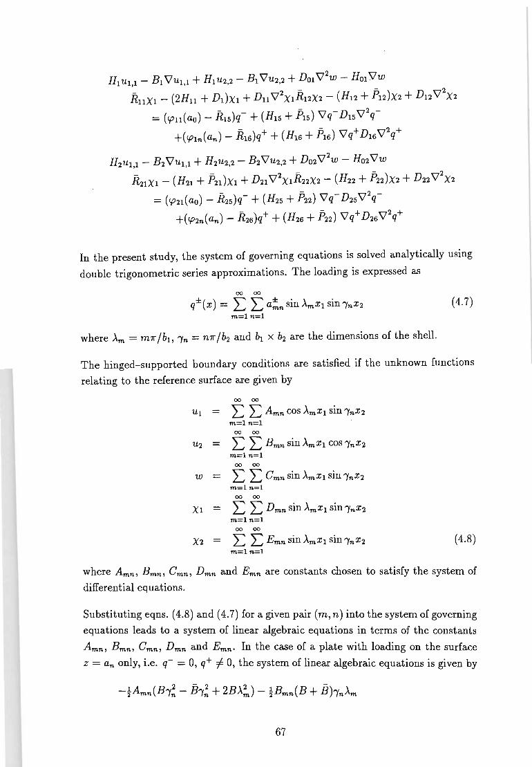
HI UI,I - BI VUI,I + HI U2,2 - BI VU2,2 + DOl V2w ~ HOI V W
RUXI - (2Hu + DI)XI + Du V 2Xl R l2 X2 - (H12 + P12 )X2 + D12 V2
X2
= (cpu(ao) - RIS)q- + (HIS + PIS) Vq- DIS V 2q-
+( CPln( an) - RI6)q+ + (H16 + P16) V q+ Dl6 V 2q+
H2UI,l - B2 VUI,I + H2U2,2 - B2 VU2,2 + D02 V 2w - H02 Vw
2 - - 2 R2lXI - (H21 + P21 )XI + D21 V Xl R22 X2 - (H22 + P22)X2 + D22 V X2
= (CP21(ao) - R 2S )q- + (H2S + P22 ) Vq- D2SV2q-- + - + 2+ +(CP2n(an) - R26 )q + (H26 + P22 ) Vq D26V q
In the present study, the system of governing equations is solved analytically using
double trigonometric series approximations. The loading is expressed as
00 00
q± (X) = L L a!n sin AmXI sin "Yn X2 (4.7) m=l n=l
where Am = m7r jbI, "Yn = n7r jb2 and bl x b2 are the dimensions of the shell.
The hinged-supported boundary conditions are satisfied if the unknown functions
. relating to the reference surface are given by
00 00
UI = L L Amn cos AmXI sin "Yn X 2 m=ln=l
00 00
U2 L L Bmn sin AmXI cos "Yn X 2 m=l n=l
00 00
w L L Cmn sin AmXI sin "Yn X 2 m=ln=l
00 00
Xl L L Dmn sin AmXI sin "Yn X 2 m=ln=l
00 00
X2 = L L Emn sin AmXI sin "Yn X 2 m=ln=l
(4.8)
where Amn , B mn , Cmn , Dmn and Emn are constants chosen to satisfy the system of differential equations.
Substituting eqns. (4.8) and (4.7) for a given pair (m, n) into the system of governing
equations leads to a system of linear algebraic equations in terms of the constants
Amn , Bmn , Cmn , Dmn and Emn. In the case of a plate with loading on the surface
z = an only, i.e. q- = 0, q+ =I 0, the system of linear algebraic equations is given by
67
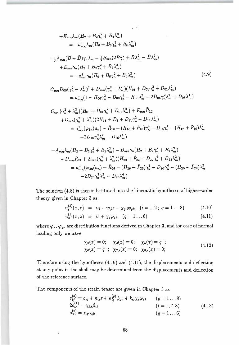
+EmnAm(H2 + B2/~ + B2A~) = -a~nAm(H6 + B6/~ + B6A~)
-tAmn(B + BhnAm - tBmn(2B/~ + BA~ - BA~) +Emnln(H2 + B2/~ + B2A~)
= -a!m/n(H6 + B6/~ + B6A~)
CmnDoob~ + A~)2 + Dmnb~ + A~)(Hol + DOI/~ + D01A~) = a~n(1- H06/~ - Dos/! - HosA~ - 2Dos/~A~ + D06A~)
Cmnb~ + A~) (HoI + DOI/~ + D01A~) + EmnRI2
+Dmnb~ + A~)(2Hll + DI + Dll/~ + DllA~)
(4.9)
- - 2 4 - 2 = a~n(<PIn(an) - RI6 - (H16 + PI6hn - DI61n - (H16 + PI6 )Am
- 2D16/~ A~ - DI6A~)
-AmnAm(H2 + B2/~ + B2A~) - Bmnln(H2 + B2/~ + B2A~) - 2 2 - 2 2
+DmnR2I + Emn(/n + Am)(H22 + P22 + D22/n + D22Am) - - 2 4 - 2
= a!m(<P2n(an) - R26 - (H26 + P26hn - D261n - (H26 + P26 )Am
- 2D26/~ A~ - D26A~)
The solution (4.8) is then substituted into the kinematic hypotheses of higher-order
theory given in Chapter 3 as
U!k)(X, z)
u~k)(x, z)
Ui - W,iZ - Xg ,itPgk (i = 1,2; 9 = 1 ... 8)
W + Xq<Pqk (q = 1 . . . 6)
( 4.10)
(4.11)
where <Pk, <pqk are distribution functions derived in Chapter 3, and for case of normal
loading only we have
X3(X) = 0; X4(X) = 0; Xs(x) = q-;
X6(X) = q+; x7Ax) = 0; XS,i(X) = 0; (4.12)
Therefore using the hypotheses (4.10) and (4.11), the displacements and deflection
at any point in the shell may be determined from the displacements and deflection
of the reference surface.
The components of the strain tensor are given in Chapter 3 as
e(k) - 1:" • • + "' ··Z + ".(g).,. k + k··X ef) ,j - ""3 ""3 "'ij 'l/g '3 qrqk (k)
2ei3 = Xt,i/3tk (k)
e33 = xqaqk
68
(g = 1. .. 8) (t = 1,7,8)
(q=1. . . 6) (4.13)
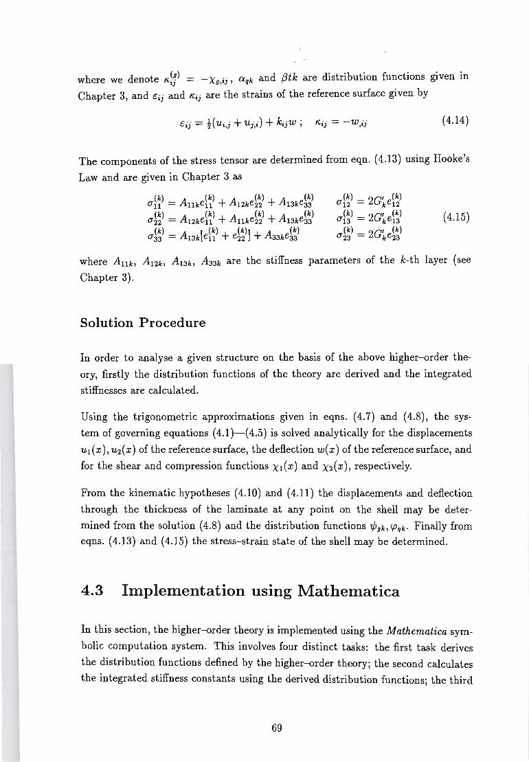
where we denote K~J) = -Xg,ij, Q:qlr; and f3tk are distribution functions given in
Chapter 3, and eij and Kij are the strains of the reference surface given by
( 4.14)
The components of the stress tensor are determined from eqn. (4.13) using Hooke's
Law and are given in Chapter 3 as
( 4.15)
where AUIr;, A 121r;, A 131r;, A331r; are the stiffness parameters of the k-th layer (see
Chapter 3).
Solution Procedure
In order to analyse a given structure on the basis of the above higher-order the
ory, firstly the distribution functions of the theory are derived and the integrated
stiffnesses are calculated.
Using the trigonometric approximations given in eqns. (4.7) and (4.8), the sys
tem of governing equations (4.1)-(4.5) is solved analytically for the displacements
Ul (x), U2( x) of the reference surface, the deflection w( x) of the reference surface, and
for the shear and compression functions Xl(X) and X2(X), respectively.
From the kinematic hypotheses (4.10) and (4.11) the displacements and deflection
through the thickness of the laminate at any point on the shell may be deter
mined from the solution (4.8) and the distribution functions tPglr;, cpqlr; . Finally from eqns. (4.13) and (4.15) the stress-strain state of the shell may be determined.
4.3 Implementation using Mathematica
In this section, the higher-order theory is implemented using the Mathematica sym
bolic computation system. This involves four distinct tasks: the first task derives
the distribution functions defined by the higher-order theory; the second calculates
the integrated stiffness constants using the derived distribution functions; the third
69
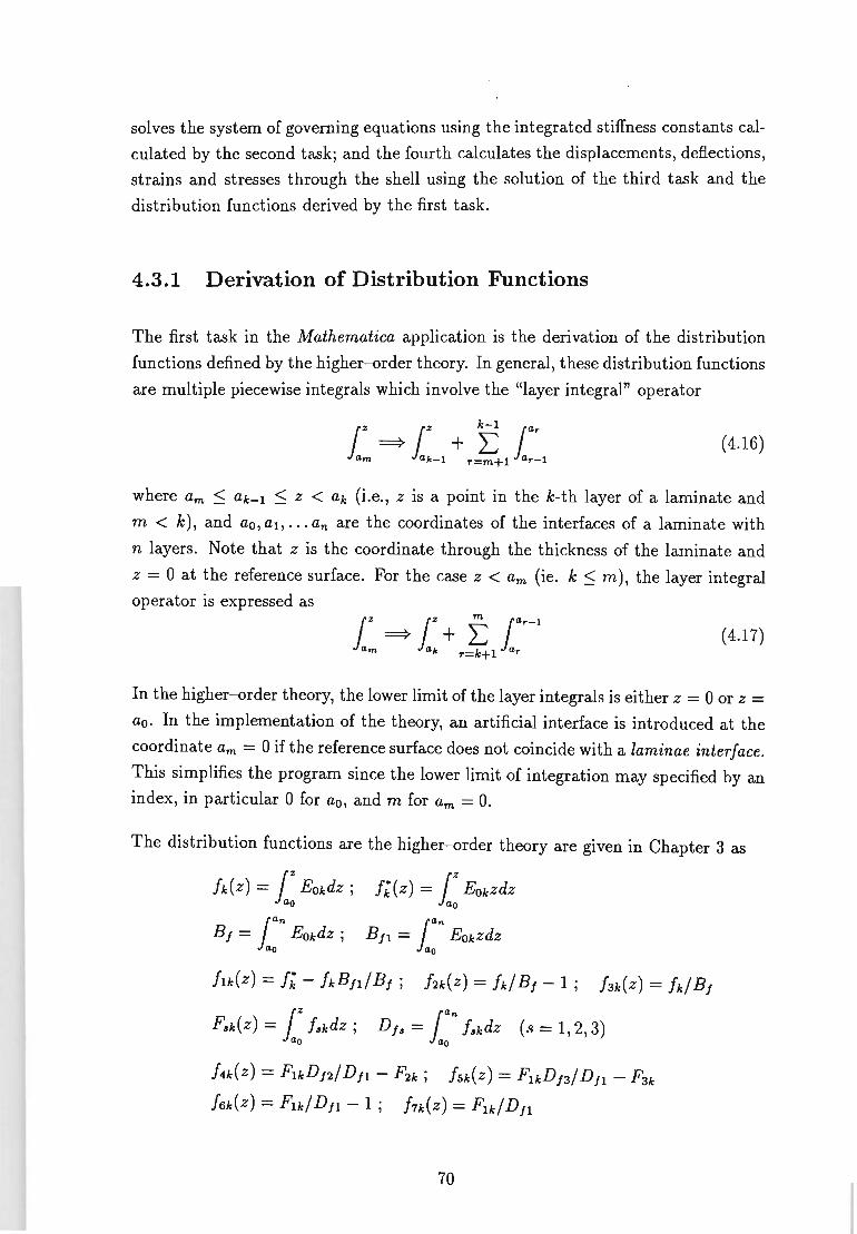
solves the system of governing equations using the integrated stiffness constants cal
culated by the second task; and the fourth calculates the displacements, deflections,
strains and stresses through the shell using the solution of the third task and the
distribution functions derived by the first task.
4.3.1 Derivation of Distribution Functions
The first task in the Mathematica application is the derivation of the distribution
functions defined by the higher-order theory. In general, these distribution functions
are multiple piecewise integrals which involve the "layer integral" operator
( 4.16)
where am :::; ak-l :::; Z < ak (i.e., z is a point in the k-th layer of a laminate and
m < k), and ao, al, ... an are the coordinates of the interfaces of a laminate with
n layers. Note that z is the coordinate through the thickness of the laminate and
z = 0 at the reference surface. For the case z < am (ie. k :::; m), the layer integral
operator is expressed as
(4.17)
In the higher-order theory, the lower limit of the layer integrals is either z = 0 or z =
ao. In the implementation of the theory, an artificial interface is introduced at the
coordinate am = 0 if the reference surface does not coincide with a laminae interface.
This simplifies the program since the lower limit of integration may specified by an
index, in particular 0 for ao, and m for am = o.
The distribution functions are the higher-order theory are given in Chapter 3 as
fZ(z) = 1% EOkZdz ao
f4k(Z) = FaDJ2/ DJl - F2k ; fSk(Z) = Fa DJ3 / Djl - F3k
f6k(Z) = Fa/ Djl - 1; f7k(Z) = Fa/ Dj1
70
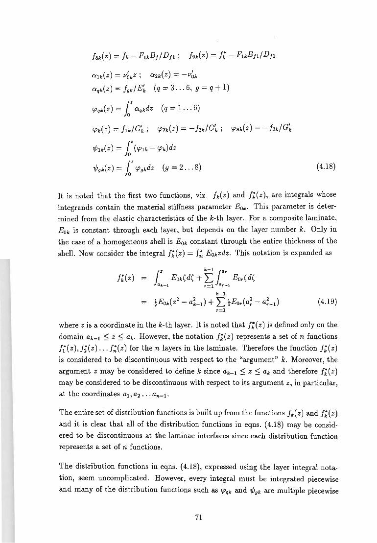
alk(Z) = lJ~kZ; a2k(Z) = -lJ~k aqk(Z) = fgk/ E~ (q = 3 ... 6, 9 =q + 1)
c,oqk( z) = 10% aqkdz (q = 1. .. 6)
c,ok(Z) = flk/G~; c,07k(Z) = - hk/G~; c,oSk(Z) = - hk/G~
.,plk(Z) = 10% (c,olk - c,ok)dz
.,pgk( z) = 10% c,ogkdz (9 = 2 ... 8) (4.18)
It is noted that the first two functions, viz. fk(Z) and fk(z), are integrals whose
integrands contain the material stiffness parameter EOk. This parameter is deter
mined from the elastic characteristics of the k-th layer. For a composite laminate,
EOk is constant through each layer, but depends on the layer number k. Only in
the case of a homogeneous shell is EOk constant through the entire thickness of the
shell. Now consider the integral fZ(z) = J:o EOkzdz. This notation is expanded as
J;(z) = 1% EOk(d( + I: l{1.r Eor(d( {1./O-1 r=l (1.r-1
k-l
- tEOk(z2 - aLl) + :L tEor(a~ - a~_l) (4.19) r=l
where z is a coordinate in the k-th layer. It is noted that fZ(z) is defined only on the
domain ak-l :::; z :::; ak. However, the notation fk(z) represents a set of n functions
J; (z ), f; (z) ... f: ( z) for the n layers in the laminate. Therefore the function fk (z ) is considered to be discontinuous with respect to the "argument" k. Moreover, the
argument z may be considered to define k since ak-l :::; z :::; ak and therefore fk(z) may be considered to be discontinuous with respect to its argument z, in particular,
at the coordinates all a2 ... an-l.
The entire set of distribution functions is built up from the functions fk(Z) and fk(z) and it is clear that all of the distribution functions in eqns. (4.18) may be consid
ered to be discontinuous at the laminae interfaces since each distribution function
represents a set of n functions.
The distribution functions in eqns. (4.18), expressed using the layer integral nota
tion, seem uncomplicated. However, every integral must be integrated piecewise
and many of the distribution functions such as cPqle and .,pgle .are multiple piecewise
71
integrals. The complexity of such integrals increases dramatically as the number of
layers in the laminate increases. Even for a three-layered shell, the task of expand
ing the functions into exact formulas for numerical computation is too overwhelming
to be attempted without the aid of symbolic computation.
In the Mathematica application, the layer integral operator J:m
(where ak-l ~ z ~
ak) is defined by the code
LayInt[fn_,m_Integer,k_Integer,z_] := Block[{r,zeta},
Return[If[m < k,
Integrate[fn[k,zeta],{zeta,a[k-1],z}] +
Sum[Integrate[fn[r,zeta],{zeta,a[r-1] ,a[r]}],{r,m+1,k-1}], If[m >= k,
Integrate[fn[k,zeta],{zeta,a[k],z}] +
Sum[Integrate[fn[r,zeta],{zeta,a[r],a[r-1]}],{r,k+1,m}], Integrate[fn[k,zeta],{zeta,a[k],z}] ]]]];
where the argument fn is a function which takes two arguments, namely a z
coordinate ( and the corresponding layer number r such that ar-l ~ ( ~ ar •
The distribution functions given in eqns. (4.18) are defined using the LayInt procedure as follows.
fsi [k_Integer ,z_] = eO[k] z; fs [k_Integer, z_] = LayInt[fsi,O,k,z]; fi [k_Integer, z_] = eO [k] ; f [k_Integer ,z_] = LayInt[fi,O,k,z];
cbf = f[n,a[n]]; cbf1 = fs[n,a[n]];
f1 [k_Integer,z_] f2 [k_Integer,z_] f3 [k_Integer,z_]
F1[k_Integer,z_] = F2[k_Integer,z_] = F3[k_Integer,z_] =
= fs[k,z] - f[k,z] cbf1/cbf; = f[k,z]/cbf - 1; = f [k,z] /cbf;
LayInt[f1,O,k,z]; LayInt[f2,O,k,z];
Laylnt[f3,O,k,z];
cdf1 = Together[F1[n,a[n]]];
cdf2 = Together[F2[n,a[n]]];
72
cdf3 = Together[F3[n,a[n]]];
f4[k_Integer,z_] = F1[k,z] cdf2/cdf1 - F2[k,z];
fS[k_Integer,z_] = Fl[k,z] cdf3/cdf1 - F3[k,z];
f6[k_Integer,z_] = F1[k,z]/cdf1 - 1;
f7[k_Integer,z_] = F1[k,z]/cdf1; f8[k_Integer,z_] = f[k,z] - F1[k,z] cbf/cdf1; f9[k_Integer,z_] = fs[k,z] - F1[k,z] cbf1/cdf1;
alp1[k_Integer,z_] = nuO[k] z;
alp2[k_Integer,z_] = -nuO[k]; alp3[k_Integer,z_] = f4[k,z]/e2[k];
alp4[k_Integer,z_] = fS[k,z]/e2[k];
alpS[k_Integer,z_] = f6[k,z]/e2[k];
alp6[k_Integer,z_] = f7[k,z]/e2[k];
vphi1[k_Integer,z_] = Laylnt[alp1,m,k,z];
vphi2[k_Integer,z_] = Laylnt[alp2,m,k,z];
vphi3[k_Integer,z_] = Laylnt[alp3,m,k,z];
vphi4[k_Integer,z_] = Laylnt[alp4,m,k,z];
vphiS[k_Integer,z_] = Laylnt[alpS,m,k,z];
vphi6[k_Integer,z_] = Laylnt[alp6,m,k,z];
vphi [k_Integer,z_] = f1[k,z]/g2[k];
vphi7[k_Integer,z_] = -f2[k,z]/g2[k];
vphi8[k_Integer,z_] = -f3[k,z]/g2[k];
psi1[k_Integer,z_] = Laylnt[vphi1,m,k,z] - Laylnt[vphi,m,k,z]; psi2[k_Integer,z_] = Laylnt[vphi2,m,k,z]; psi3[k_Integer,z_] = Laylnt[vphi3,m,k,z]; psi4[k_Integer,z_] = Laylnt[vphi4,m,k,z]; psiS[k_Integer,z_] = Laylnt[vphiS,m,k,z]; psi6[k_Integer,z_] = Laylnt[vphi6,m,k,z]; psi7[k_Integer,z_] = Laylnt[vphi7,m,k,z];
psi8[k_Integer,z_] = Laylnt[vphi8,m,k,z];
where n is the number of layers, a[O], a[l] ... a[n] are the coordinates of the
laminae interfaces, and m is the index of the laminae interface that coincides with
the reference surface such that a em] = o. Also, eO [k] , nuO [k] and g2 [k] are elastic
73

characteristics of the k-th layer.
The above Mathematica code defines the distribution functions for a generallami
nate. In order the derive the distribution functions for the three-layered symmetri
cally laminated shell, we define the following elastic and geometric constants
n = 4;
m = 2;
a[O]
a[l]
a[2]
a[3]
a[4]
el [1]
e2[lJ
el [2]
e2[2J
el [3J
e2[3]
el [4J
e2[4]
nuO
eO
del
delll
del12
del13
de133
aU
a12
a13
a33
= - h/2;
= - h hr;
= 0 ;
= h hr;
= h/2;
= bel; nul [lJ = bnul; gl [lJ = bgl;
= be2; nu2 [lJ = bnu2; g2[lJ = bg2;
= fel; nul [2] = fnul; gl [2] = fgl;
= fe2; nu2 [2J = fnu2; g2[2J = fg2;
= fel; nul [3J = fnul; gl [3J = fgl;
= fe2; nu2 [3] = fnu2; g2[3] = fg2;
= bel; nul [4J = bnul; g1[4J = bgl;
= be2; nu2 [4] = bnu2; g2[4] = bg2;
[k_Integer] = el[k] nu2[k] / (e2[k] (1 - nul[kJ)); [k_IntegerJ = el[kJ / (1 - nul[k]-2);
[k_Integer] = (1 + nul[k]) (1 - nul[k] -
2 nu2[kJ-2 el[kJ/e2[kJ) / (el [kJ -2 e2 [k]) ; [k_IntegerJ = (1 - nu2[k]-2 el[k]/e2[k])/(el[k] e2[k]); [k_Integer] = (nul[k] + nu2[k]-2 el[k]/e2[k]) / (el[k] e2 [k]) ; [k_Integer] = nu2[k] (1+ nul[k]) / (el[k] e2 [k]) ; [k_Integer] = (1 - nul[k]-2) / el[k]-2;
[k_IntegerJ = delll[kJ/del[k]; [k_Integer] = del12[k]/del[k];
[k_Integer] = del13[k]/del[k];
[k_IntegerJ = de133[kJ/del[kJ;
where h is the thickness of the shell and hr is a parameter which determines the
thickness of the core layer (0 ~ hr ~ t). Also, el [k], e2 [kJ, nul [k], nu2 [k] ,
gl [kJ, g2 [kJ are the elastic characteristics E, E', 11, 11', G, G' of the transversely
74
isotropic k-th layer; and in particular bel, be2, bnul, bnu2, bgl, bg2 are the elastic
characteristics of the surface (or bearing) layers of the sandwich shell, and fel, fe2,
fnul, fnu2, fgl, fg2 are the elastic characteristics of the core (or filler) layer.
Once the material and geometric parameters have been specified, the distribution
functions may be derived for each layer by the code
Do [fl [r, z_] = fl [r ,z] , {r, 1 ,n}]
Do [f2 [r ,z_] = f2 [r ,z] , {r,l,n}]
Do[f3[r,z_] = f3 [r ,z] , {r, 1 ,n}]
Do [Fl [r ,z_] = F1[r ,z] , {r,l,n}]
Do [F2 [r , z_] = F2 [r ,z] , {r,l ,n}]
Do [F3 [r , z_] = F3[r,z], {r,l,n}]
Do[f4[r,z_] = f4[r,z], {r,l,n}]
Do[f5[r,z_] = f5[r,z], {r,l,n}]
Do[f6[r,z_] = f6[r,z], {r,l,n}]
Do [alpl [r ,z_] = alpl [r ,z] , {r,l,n}] ;
Do [alp2[r,z_] = alp2[r,z], {r, 1 ,n}] ;
Do [alp3[r,z_] = alp3 [r ,z] , {r, 1 ,n}] ;
Do [alp4[r,z_] = alp4 [r ,z] , {r,l ,n}];
Do [alp5 [r, z_] = alp5 [r ,z] , {r, 1 ,n}] ;
Do [alp6[r,z_] = alp6 [r ,z] , {r,l,n}] ;
Do[betal[r,z_] = betal[r,z],{r,l,n}]
Do[beta7[r,z_] = beta7[r,z],{r,l,n}]
Do[beta8[r,z_] = beta8[r,z],{r,l,n}]
Do[vphil[r,z_] = vphil[r,z],{r,l,n}];
Do[vphi2[r,z_] = vphi2[r,z],{r,l,n}];
Do[vphi3[r,z_] = vphi3[r,z],{r,l,n}];
Do[vphi4[r,z_] = vphi4[r,z],{r,l,n}];
Do[vphi5[r,z_] = vphi5[r,z],{r,l,n}];
Do[vphi6[r,z_] = vphi6[r,z],{r,l,n}];
Do[psil[r,z_] = psil[r,z], {r,l,n}];
Do [psi2[r,z_] = psi2[r,z], {r,l,n}];
75
Do [psi3 [r, z_] = psi3[r,z] , {r, 1 ,n}] ;
Do [psi4 [r ,z_] = psi4[r,z], {r, 1 ,n}] ;
Do [psi5 [r, z_] = psi5[r,z], {r,l ,n}] ;
Do [psi6 [r, z_] = psi6[r,z] , {r,l,n}] ;
Do [psi 7 [r, z_] = psi7[r,z] , {r, 1 ,n}] ;
Do [psi8 [r ,z_] = psi8[r,z] , {r, 1 ,n}] ;
The computational efficiency of the above code heavily depends on the sequence of
the derivations. For example, because functions "pgk are piecewise integrals of the
functions r.pqk, the latter are derived first so that they are ready to be employed in
the derivations of the functions "pgk. If the sequence were reversed, the functions
r.pqk would be derived by Mathematica repetitively.
These distribution functions are required for the calculation of the integrated stiff
ness constants which appear in the system of governing equations, and for the deter
mination of the displacements, deflection, strains and stresses through the thickness
of the laminate.
4.3.2 Derivation of Integrated Stiffnesses
The second task of the Mathematica application is the calculation of the integrated
stiffnesses using the distribution functions derived by the first task.
The integrated stiffness constants are definite layer integrals through the thickness
of the laminate from ao to an. Their integrands contain stiffness parameters which
depend on the layer number and distribution functions which are "discontinuous" at
the laminae interfaces. In general, the integrated stiffnesses are multiple piecewis~
integrals which even for a three-layered laminate are too tedious to calculate exactly
without the aid of symbolic computation.
76
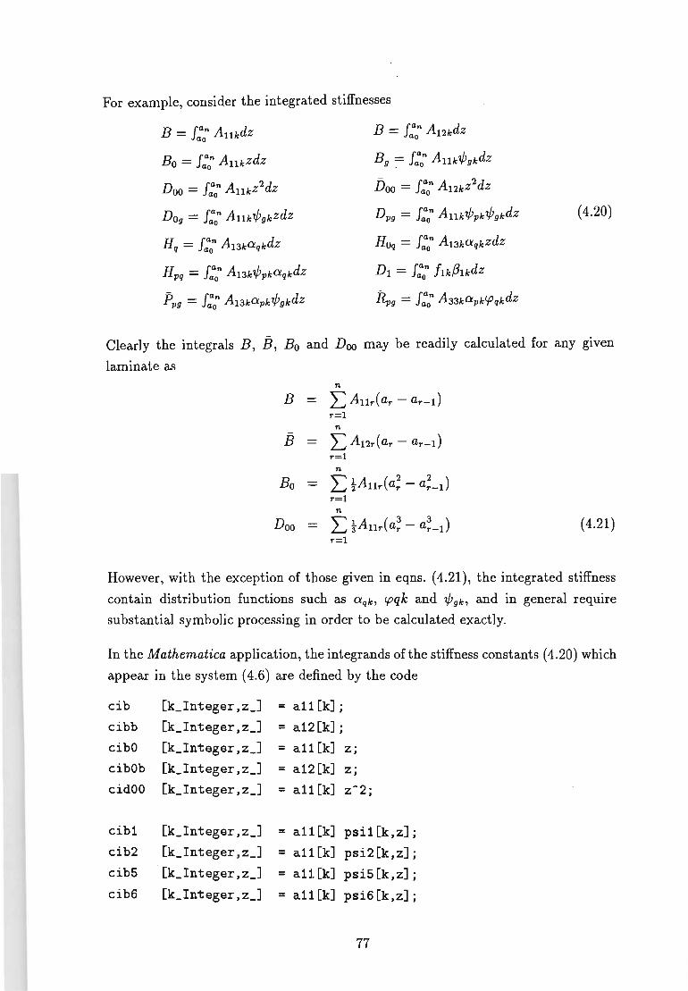
For example, consider the integrated stiffnesses
B = I:on Allkdz 13 = I:; A 12kdz
Bo = I:on Allkzdz Bg . I:on AllktPgkdz
Doo = I:an AllkZ2dz Doo = I:on A12kZ2dz
Dog = I:on A1lktPgkZdz Dpg = I:on AllktPpktPgkdz ( 4.20)
Hq = I:on A13kaqkdz Hoq = I:on A13kaqkZdz
Hpq = I:on A13ktPpkaqkdz Dl = I:on flkf3lk dz
Ppg = I:on A13kapktPgkdz 14g = I:on A33kapk<Pqkdz
Clearly the integrals B, 13, Bo and Doo may be readily calculated for any given
laminate as n
B LAllr(ar - ar-l) r=l
n
13 - LA12r(ar - ar-l) r=l
n
Bo L tAllr( a; - a;_l) r=l
n
Doo L tAllr( a~ - a~_l) (4.21 ) r=l
However, with the exception of those given in eqns. (4.21), the integrated stiffness
contain distribution functions such as aqk' <pqk and tPgk, and in general require
substantial symbolic processing in order to be calculated exactly.
In the Mathematica application, the integrands of the stiffness constants (4.20) which
appear in the system (4.6) are defined by the code
cib [k_Integer .z_] = a11 [k];
cibb [k_Integer . z_] = a12 [k] ;
cibO [k_Integer. z_] = all[k] z· • cibOb [k_Integer . z_] = a12 [k] z;
cidOO [k_Integer . z_] = a11 [k] z-2;
cibl [k_Integer . z_] = a11 [k] psil [k.z] ;
cib2 [k_Integer . z_] = a11 [k] psi2[k.z];
cib5 [k_Integer . z_] = all [k] psi5[k.z];
cib6 [k_Integer . z_] = all [k] psi6[k.z];
77
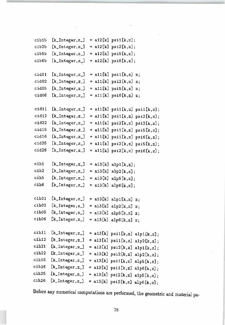
ciblb [k_Integer, z_] = a12 [k] psi! [k,z] ;
cib2b [k_Integer ,z_] = a12 [k] psi2 [k,z] j
cib5b [k_Integer, z_] = a12[k] psi5[k,z]j
cib6b [k_Integer , z-:] = a12 [k] psi6[k,z]j
cidOl [k_Integer , z_] = a11 [k] psi! [k,z] z· , cid02 [k_Integer , z_] = al1[k] psi2 [k,z] Zj
cid05 [k_Integer , z_] = a11 [k] psi5 [k,z] z· , cid06 [k_Integer , z_] = a11 [k] psi6 [k,z] z· ,
cidll [k_Integer , z_] = a11 [k] psil [k,z] psil [k,z] ;
cid12 [k_Integer , z_] = a11 [k] psi! [k,z] psi2 [k,z] j
cid22 [k_Integer , z_] = a11 [k] psi2 [k,z] psi2 [k,z] ;
cid15 [k_Integer , z_] = a11 [k] psi! [k,z] psi5 [k,z] ;
cid16 [k_Integer , z_] = a11 [k] psil[k,z] psi6 [k,z] j
cid25 [k_Integer , z_] = a11 [k] psi2 [k,z] psi5 [k,z] ;
cid26 [k_Integer , z_] = a11 [k] psi2 [k,z] psi6[k,z];
cihl [k_Integer , z_] = a13 [k] alpl[k,z];
cih2 [k_Integer , z_] = a13 [k] alp2[k,z];
cih5 [k_Integer , z_] = a13 [k] alp5[k,z];
cih6 [k_Integer , z_] = a13[k] alp6[k,z];
cihOl [k_Integer , z_] = a13[k] alpl [k,z] z· , cih02 [k_Integer , z_] = a13 [k] alp2 [k,z] z· , cih05 [k_Integer , z_] = a13 [k] alp5[k,z] z· , cih06 [k_Integer , z_] = a13[k] alp6[k,z] z;
cihll [k_Integer , z_] = a13[k] psi! [k,z] alpl [k,z] ; cih12 [k_Integer , z_] = a13 [k] psi! [k,z] alp2 [k,z] ; cih21 [k_Integer , z_] = a13[k] psi2 [k,z] alpl [k,z] ; cih22 [k_Integer , z_] = a13[k] psi2 [k,z] alp2[k,z]; cih15 [k_Integer , z_] = a13 [k] psi! [k,z] alp5 [k,z] ; cih16 [k_Integer , z_] = a13[k] psi! [k,z] alp6[k,z]; cih25 [k_Integer , z_] = a13[k] psi2 [k,z] alp5 [k,z] ; cih26 [k_Integer , z_] = a13[k] psi2 [k,z] alp6[k,z];
Before any numerical computations are performed, the geometric and material pa-
78
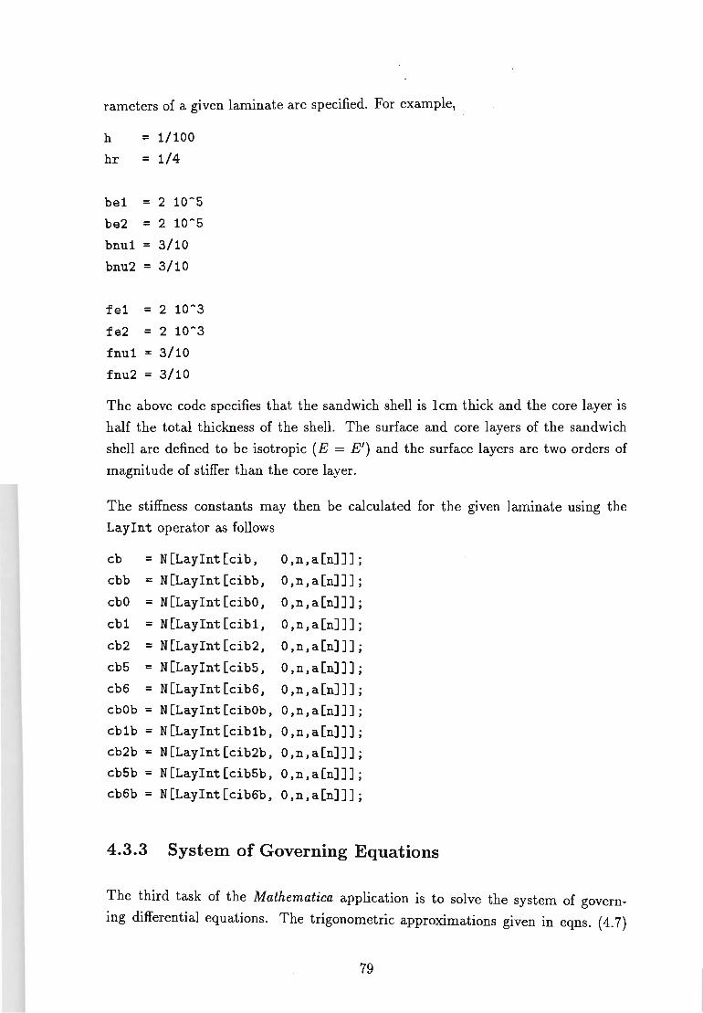
rameters of a given laminate are specified. For example,
h = 1/100
hr = 1/4
bel = 2 10 A 5
be2 = 2 10 A 5
bnul = 3/10
bnu2 = 3/10
fel = 2 10 A 3
fe2 = 2 10 A 3
fnul = 3/10
fnu2 = 3/10
The above code specifies that the sandwich shell is lcm thick and the core layer is
half the total thickness of the shell. The surface and core layers of the sandwich
shell are defined to be isotropic (E = E') and the surface layers are two orders of
magnitude of stiffer than the core layer.
The stiffness constants may then be calculated for the given laminate using the
Laylnt operator as follows
cb = N[Laylnt[cib, o ,n , a En] ]] ;
ebb = N [Laylnt [cibb, o ,n , a En] ]] ;
cbO = N[Laylnt[ci bO, o ,n , a En] ]] ;
cbl = N[Laylnt[cibl, o ,n , a En] ]] ;
cb2 = N[Laylnt[ci b2, o , n , a En] ] ] ;
cb5 = N[Laylnt[ci b5, o , n , a En] ]] ;
cb6 = N[Laylnt[cib6, o , n , a En] ]] ;
cbOb = N[Laylnt[ci bOb, o • n • a En] ]] ;
cblb = N[Laylnt[ciblb, o ,n , a En] ]] ;
cb2b = N[Laylnt[cib2b, o ,n , a En] ]] ;
cb5b = N[Laylnt[cib5b, o ,n , a En] ]] ;
cb6b = N[Laylnt[cib6b, o ,n , a En] ]] ;
4.3.3 System of Governing Equations
The third task of the Mathematica application is to solve the system of govern
ing differential equations. The trigonometric approximations given in eqns. (4.7)
79
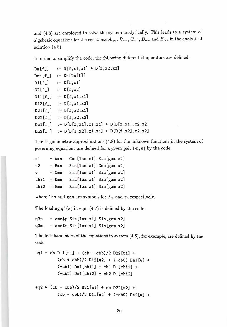
and (4.8) are employed to solve the system analytically. This leads to a system of
algebraic equations for the constants Amn, Bmn, Cmn , Dmn and Emn in the analytical
solution (4.8).
In order to simplify the code, the following differential operators are defined:
Dn[f_] := D[f,xl ,xl] + D [f , x2 , x2]
Dnn[f_] := Dn[Dn [f]]
Dl [f_] := D[f,xl]
D2 [f_] := D[f ,x2]
Dl1 [f_] := D[f ,xl,xl]
D12 [f_] := D[f,xl,x2]
D21 [f_] := D[f,x2,xl]
D22 [f_] : = D [f , x2 , x2]
Dn1[f_] : = D [D [f ,xl] ,xl,xl] + D[D[f,xl],x2,x2]
Dn2 [f_] := D[D[f,x2],xl,xl] + D[D[f,x2] ,x2,x2]
The trigonometric approximations (4.8) for the unknown functions in the system of
governing equations are defined for a given pair (m, n) by the code
ul = Amn Cos [ lam xl] Sin[gam x2]
u2 = Bmn Sin [lam xl] Cos [gam x2]
w = Cmn Sin [lam xl] Sin[gam x2]
chii = Dmn Sin[lam xl] Sin[gam x2]
chi2 = Emn Sin [lam xl] Sin[gam x2]
where lam and gam are symbols for Am and In respectively.
The loading q± (x) in eqn. (4.7) is defined by the code
q3p = amn$p Sin [lam xl] Sin [gam x2]
q3m = amn$m Sin[lam xl] Sin [gam x2]
The left-hand sides of the equations in system (4.6), for example, are defined by the
code
eql = cb Dll[ul] + (cb - cbb)/2 D22[ul] +
(cb + cbb)/2 D12[u2] + (-cbO) Dnl[w] +
(-cbl) Dnl[chil] + chl Dl[chil] +
(-cb2) Dnl[chi2] + ch2 Dl[chi2]
eq2 = (cb + cbb)/2 D2l[ul] + cb D22[u2] +
(cb - cbb)/2 Dll[u2] + (-cbO) Dn2[w] +
80
(-cbl) Dn2[chil] + chl D2[chil] +
(-cb2) Dn2[chi2] + ch2 D2[chi2]
eq3 = (-cbO) Dnl[ul] + (-cbO) Dn2[u2] + cdOO Dnn[w] +
cdOl Dnn[chil] + (-chOl) Dn[chil] +
cd02 Dnn[chi2] + (-ch02) Dn[chi2]
eq4 = (-cbl) Dnl[ul] + chl Dl[ul] + (-cbl) Dn2[u2] +
chl D2[u2] + cdOl Dnn[w] + (-chOl) Dn[w] +
cdll Dnn[chil] + (-chsll) Dn[chil] + crbll chil +
cd12 Dnn[chi2] + (-chs12) Dn[chi2] + crb12 chi2
eq5 = (-cb2) Dnl[ul] + ch2 Dl[ul] + (-cb2) Dn2[u2] +
ch2 D2[u2] + cd02 Dnn[w] + (-ch02) Dn[w] +
cd2l Dnn[chil] + (-chs2l) Dn[chil] +
crb2l chil + cd22 Dnn[chi2] +
(-chs22) Dn[chi2] + crb22 chi2
and the right-hand sides by
rl = cb6 Dnl[q3p] - ch6 Dl[q3p]
r2 = cb6 Dn2[q3p] - ch6 D2[q3p]
r3 = q3p + ch06 Dn[q3p] - cd06 Dnn[q3p]
r4 = crbs16 q3p + chs16 Dn[q3p] - cd16 Dnn[q3p]
r5 = crbs26 q3p + chs26 Dn[q3p] - cd26 Dnn[q3p]
rl += cb5 Dnl[q3m] - ch5 Dl[q3m]
r2 += cb5 Dn2[q3m] - ch5 D2[q3m]
r3 += q3m + ch05 Dn[q3m] - cd05 Dnn[q3m]
r4 += crbs15 q3m + chs15 Dn[q3m] - cd15 Dnn[q3m]
r5 += crbs25 q3m + chs25 Dn[q3m] - cd25 Dnn[q3m]
The expressions for the left-hand sides of the system of equations are simplified into
algebraic expressions in terms of the unknowns Amn , Bmn, Cmn , Dmn and Emn by
the code
eqal = Cancel[eql/Cos[lam xl]/Sin[gam x2]]
eqa2 = Cancel[eq2/Sin[lam xl]/Cos[gam x2]]
eqa3 = Cancel[eq3/Sin[lam xl]/Sin[gam x2]]
eqa4 = Cancel[eq4/Sin[lam xl]/Sin[gam x2]]
eqa5 = Cancel[eq5/Sin[lam xl]/Sin[gam x2]]
81
and the right-hand sides by
ra1 = Cancel [r1/Cos[lam x1]/Sin[gam x2]]
ra2 = Cancel[r2/Sin[lam x1]/Cos[gam x2]]
ra3 = Cancel[r3/Sin[lam x1]/Sin[gam x2]]
ra4 = Cancel[r4/Sin[lam x1]/Sin[gam x2]]
ra5 = Cancel[r5/Sin[lam x1]/Sin[gam x2]]
The system of algebraic equations may now be solved by the code
amn$p = -qO
amn$m = 0
lambda[mw_,nw_] := mw Pi/a1;
gamma [mw_,nw_] := nw Pi/a2;
mw = nw = 1;
lam = lambda[mw,nw]; gam = gamma[mw,nw]
soln = N[Solve[{eqa1 == ra1, eqa2 -- ra2, eqa3 == ra3, eqa4 == ra4, eqa5 == ra5}, {Amn,Bmn,Cmn,Dmn,Emn} ]] ;
{Ac[mw,nw]} = Amn /. soln;
{Bc[mw,nw]} = Bmn /. solnj
{Cc[mw,nw]} = Cmn /. soln; {Dc[mw,nw]} = Dmn /. solnj {Ec[mw,nw]} = Emn / . soln;
where it is specified that a sinusoidal load of amplitude qO is acting on the top surface of the shell.
Finally, the solution is defined as
u1[x1_ ,x2_] := Ac[mw,nw] Cos [lam xi] Sin[gam x2]j u2 [xC ,x2_] := Bc[mw,nw] Sin [lam xi] Cos[gam x2]j w[xC,x2_] := Cc[mw,nw] Sin [lam xi] S in [gam x2] ; chi1 [xC ,x2_] := Dc[mw,nw] Sin [lam xi] Sin [gam x2] ; chi2 [x1_ ,x2_] := Ec[mw,nw] Sin [lam xi] Sin[gam x2]j
82

4.3.4 Stresses and Strains
The fourth task of the Mathematica application is the calculation of the displace
ments, deflection, strains and stresses through the thickness of the laminate from
the solution (4.8) using the kinematic hypotheses of the higher-order theory.
The kinematic hypotheses given in eqns. (4.10) and (4.11) and the strains given in
eqns. (4.13) include the solution (4.8) which is determined by the third task of the
application, and distribution functions of the higher-order theory which are derived
by the first task.
In order to simplify the code, a notation for the derivatives of Ui (x), W, Xgk are
defined, for example
w$l [xC ,x2_] := D[w[xdl,xd2],xdl] /. {xdl -) xl,
w$2 [xC ,x2_] := D[w[xdl,xd2] ,xd2] /. {xdl -) xl,
w$11 [xl_ ,x2_] := D[w[xdl,xd2] ,xdl,xdl] /. {xdl -) xl,
w$12 [xC ,x2_] := D[w[xdl,xd2],xdl,xd2] /. {xdl -) xl,
w$22[xl_,x2_] := D[w[xdl,xd2],xd2,xd2] /. {xdl -) xl,
ul$1[xl_,x2_] := D[ul[xdl,xd2],xdl] /. {xdl -) xl,
ul$2[xl_,x2_] := D[ul[xdl,xd2],xd2] /. {xdl -> xl, u2$1 [xC ,x2_] := D[u2[xdl,xd2],xdl] /. {xdl -> xl, u2$2[xl_,x2_] := D[u2[xdl,xd2],xd2] /. {xdl -) xl,
chil$l [xl_ ,x2_] := D[chil[xdl,xd2],xdl] /. {xdl -> xl, chi2$1 [xl_ ,x2_] := D[chi2[xdl,xd2],xdl] / . {xdl -> xl, chi5$1 [xC ,x2_] := D[chi5[xdl,xd2],xdl] /. {xdl -> xl, chi6$1 [xl_ ,x2_] := D[chi6[xdl,xd2],xdl] / . {xdl -> xl,
where, for example, chi2$1 denotes the derivative X2,1.
The displacements (4.10) and deflection (4.11) are defined by
ulk[xl_,x2_,k_Integer,z_] = Expand[
ul[xl,x2] - w$1[xl,x2] z -
chil$1[xl,x2] psil[k,z] - chi2$1[xl,x2] psi2[k,z]
chi5$1[xl,x2] psi5[k,z] - chi6$1[xl,x2] psi6[k,z] ] ;
u2k[xl_,x2_,k_Integer,z_] = Expand[
u2[x1,x2] - w$2[xl,x2] z -
chil$2[xl,x2] psil[k,z] - chi2$2[xl,x2] psi2[k,z] _
83
xd2 -) x2};
xd2 -) x2};
xd2 -) x2};
xd2 -) x2};
xd2 -) x2};
xd2 -> x2};
xd2 -) x2};
xd2 -> x2};
xd2 -> x2};
xd2 -> x2};
xd2 -> x2};
xd2 -) x2};
xd2 -) x2};
chi5$2[xl,x2] psi5[k,z] - chi6$2[xl,x2] psi6[k,zl
] ;
u3k[xl_,x2_,k_Integer,z_] :=
v[xl,x2] + chil[xl,x2] vphil[k,z] + chi2[xl,x2] vphi2[k,z] +
chi5[xl,x2] vphi5[k,z] + chi6[xl,x2] vphi6[k,z]
The strains of the reference surface given by eqns. (4.14) are calculated by the code
serll[xl_,x2_] := N[(ul$1[xl,x2] + ul$1[xl,x2])/2 + kll v[xl,x2]];
ser22 [xl_,x2_] := N[(u2$2[xl,x2] + u2$2[xl,x2])/2 + k22 v[xl,x2]];
ser12[xl_,x2_] := N[(ul$2[xl,x2] + u2$1[xl,x2])/2 + k12 v[xl,x2]];
skrll[xl_,x2_] := N[-v$ll[xl,x2]];
skr22[xl_,x2_] := N[-v$22[xl,x2]];
skr12[xl_,x2_] := N[-v$12[xl,x2]];
skr2l [xl_,x2_] := N[-v$2l[xl,x2]];
The strains through the thickness given by eqns. (4.13) are calculated by the code
sell[xl_,x2_,k_Integer,z_] := Expand[N[
serll[xl,x2] + skrll[xl,x2] z -
chil$l1 [xl ,x2] psil [k,z] - chi2$11 [xl ,x2] psi2 [k,z] -
chi5$11[xl,x2] psi5[k,z] - chi6$11[xl,x2] psi6[k,z] +
kll (chil[xl,x2] vphil[k,z] + chi2[xl,x2] vphi2[k,z] +
chi5[xl,x2] vphi5[k,z] + chi6[xl,x2] vphi6[k,z]) ]];
se22 [xl_,x2_,k_Integer,z_] := Expand[N[
ser22[xl,x2] + skr22[xl,x2] z -
chil$22[xl,x2] psil[k,z] - chi2$22[xl,x2] psi2[k,z] -
chi5$22[xl,x2] psi5[k,z] - chi6$22[xl,x2] psi6[k,z] +
k22 (chil[xl,x2] vphil[k,z] + chi2[xl,x2] vphi2[k,z] +
chi5[xl,x2] vphi5[k,z] + chi6[xl,x2] vphi6[k,z]) ]] ;
se12[xl_,x2_,k_Integer,z_] := Expand[N[
ser12[xl,x2] + skr12[xl,x2] z -
chil$12[xl,x2] psil[k,z] - chi2$12[xl,x2] psi2[k,z]
chi5$12[xl,x2] psi5[k,z] - chi6$12[xl,x2] psi6[k,z]
84
]];
se13[xl_,x2_,k_Integer,z_] := Expand[N[chil$1[xl,x2] betal[k,z]/2]];
se23[xl_,x2_,k_Integer,z_] := Expand[N[chil$2[xl,x2] betal[k,z]/2]];
se33[xl_,x2_,k_Integer,z_] := Expand[N[chil[xl,x2] alpl[k,z] +
chi2[xl,x2] alp2[k,z] + chi5[xl,x2] alp5[k,z] +
chi6[xl,x2] alp6[k,z]
]];
Finally, the stresses through the thickness given by eqns. (4.15) are calculated by
the code
ssll[xl_,x2_,k_Integer,z_] := Expand[N[all[k] sell[xl,x2,k,z] +
a12[k] se22[xl,x2,k,z] + a13[k] se33[xl,x2,k,z]]];
ss22[xl_,x2_,k_Integer,z_] := Expand[N[a12[k] sell[xl,x2,k,z] +
all[k] se22[xl,x2,k,z] + a13[k] se33[xl,x2,k,z]]];
sS33[xl_,x2_,k_Integer,z_] := Expand[N[a13[k] sell[xl,x2,k,z] +
a13[k] se22[xl,x2,k,z] + a33[k] se33[xl,x2,k,z]]];
ss12[xl_,x2_,k_Integer,z_] := Expand[N[2 g2[k] se12[xl,x2,k,z]]];
ss13[xl_,x2_,k_Integer,z_] := Expand[N[2 g2[k] se13[xl,x2,k,z]]];
ss23[xl_,x2_,k_Integer,z_] := Expand[N[2 g2[k] se23[xl,x2,k,z]]];
4.4 Homogeneous Shell
. In order to illustrate the higher-order model, a transversely isotropic homogeneous
shell is considered. The homogeneous shell is modelled as a special case of a sandwich
shell with the same elastic constants for the surface and core layers.
As given in Appendix A, the distribution functions for the normal displacements are
derived by Mathematica as
Ell' ____ Z2 2E'(1 - II)
Ell' E'(l _lI)z
_1_ (z4 _ 2z3 _ Z2 hZ) 4E' h2 3h 2 + 2
85
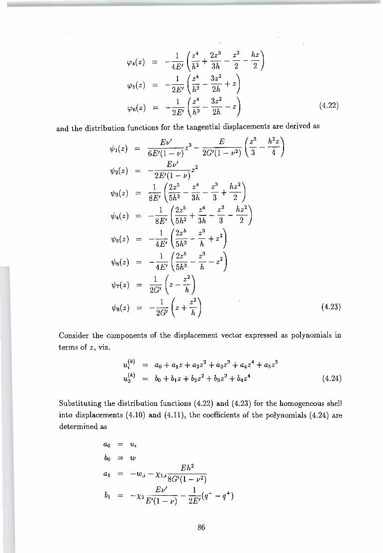
I',(z) - 4~' (~> ~: - z; _ h;) 4?s(z) -2~' (~: - ~~ +Z) 4?6( Z) = - 2~' (~: - ~: - Z) ( 4.22)
and the distribution functions for the tangential displacements are derived as
Ell' 3 E (Z3 h2Z) 1/Jt(Z) 6E'(1- II)Z - 2G'(1 -112) 3" - 4
Ell' ____ z2 2E'(1 - II)
_1_ ( 2ZS _ Z4 _ Z3 hZ2) tP3(Z) - 8E' 5h2 3h 3 + 2
__ 1_ (2ZS Z4 _ z3 _ hZ2) 8E' 5h2 + 3h 3 2
tPS(Z) 1 (2ZS Z3 2) - 4E' 5h3 - h + Z
__ 1 (2ZS _ Z3 _ Z2) 4E' 5h3 h
2~' (Z - ~) ( 4.23)
Consider the components of the displacement vector expressed as polynomials in terms of z, viz.
(k) u· ,
(k) U 3
ao + alZ + a2z2 + a3z3 + a4z4 + aszs
- bo + bIZ + b2z2 + b3z3 + b4z4 ( 4.24)
Substituting the distribution functi~ns (4.22) and (4.23) for the homogeneous shell
into displacements (4.10) and (4.11), the coefficients of the polynomials (4.24) are determined as
bo W
-W,i - XI,i 8G'(1 _ 112)
Ell' 1 -X2 E'(l - II) - 2E,(q- - q+)
86
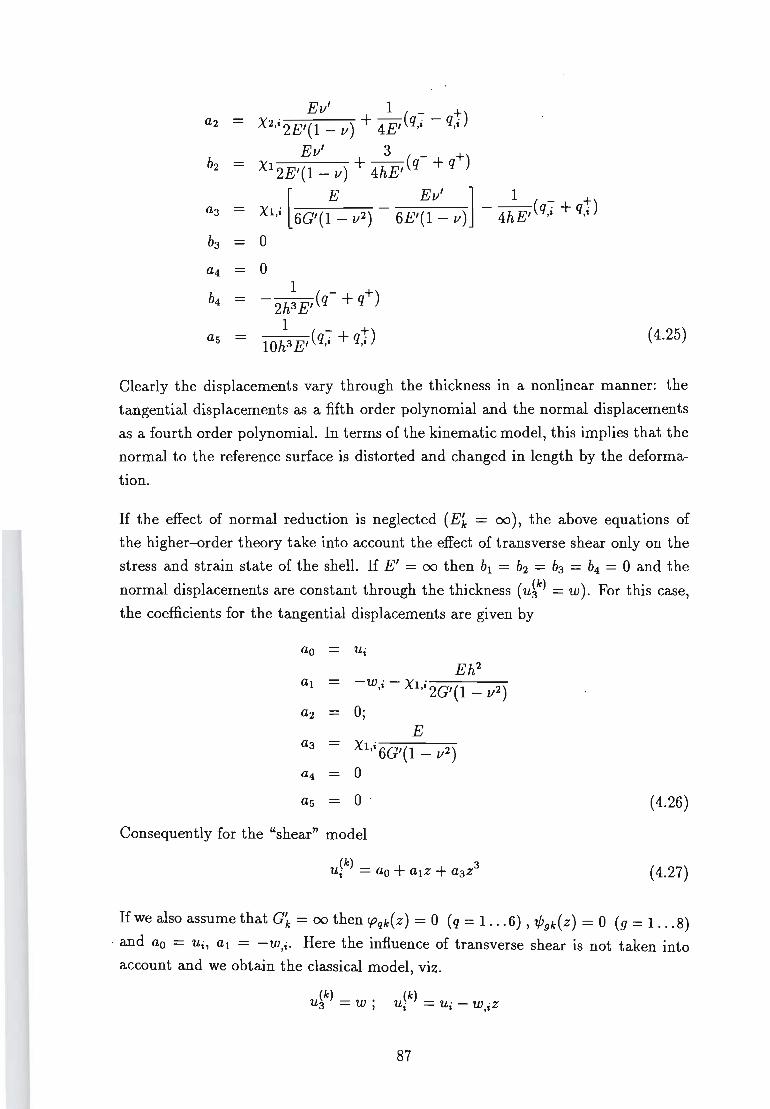
Ev' 1 X2 ,i2E'(1 - v) + 4E,(q~ - q~)
Ev' 3 XI 2E'(1_ v) + 4hE,(q-+ q+)
Xl,' [6G'(:- V2 ) - 6E'~V~ V)]- 4:E,(q~ + q~) o o
1 (_ +) - 2h3 E' q + q
1 _ +) lOh3 E,(q,i + q,i (4.25)
Clearly the displacements vary through the thickness in a nonlinear manner: the
tangential displacements as a fifth order polynomial and the normal displacements
as a fourth order polynomial. In terms of the kinematic model, this implies that the
normal to the reference surface is distorted and changed in length by the deforma
tion.
If the effect of normal reduction is neglected (Ek = 00), the above equations of
the higher-order theory take into account the effect of transverse shear only on the
stress and strain state of the shell. If E' = 00 then bl = b2 = b3 = b4 = 0 and the
normal displacements are constant through the thickness (u~k) = w). For this case,
the coefficients for the tangential displacements are given by
ao Ui Eh2
al -W,i - XI ,i 2G'(1 _ v2)
a2 O· , E
a3 - XI ,i 6G'(1 _ v2)
a4 - 0
as - 0 (4.26)
Consequently for the "shear" model
(4.27)
If we also assume that G~ = 00 then cpqk(Z) = 0 (q = 1 .. . 6) , "pgk(Z) = 0 (g = 1 ... 8)
. and ao = Ui, al = -W,i· Here the influence of transverse shear is not taken into account and we obtain the classical model, viz.
u(k) - w· u(k) = u · - w .z 3 - 'I 1 ,I
87
It is noted that the higher-order model described above considers the effect of normal
reduction caused by the external loads as well as Poisson's ratio effects including
the elongation or reduction of the reference surface.
If Poisson's ratio effect is neglected (X2 = 0) and the influence of the external loads
in the kinematic hypotheses (4.10) and (4.11) is neglected (Xg = 0, 9 = 3 ... 8), then
the coefficients of u~k) in eqn. (4.24) vanish except for
bo w Ev'
(4.28) X1 2E'(1 - v)
In this simplified case, the distribution of the displacements through the thickness
may be inaccurate. For example, if only one external surface of a symmetrically
laminated shell is under load, then the displacements uC;) would be symmetric with
respect to the middle surface, which is obviously not the true behaviour.
4.5 Special Purpose Symbolic Computation
The objective of the present study is to implement the higher-order theory for the
general case, i.e. for a laminate with any number of layers, and in this respect the
use of a general purpose system is found to be impractical due to the unimpressive
computational efficiency of such systems.
Therefore special purpose symbolic computation software is developed in the C
programming language for the computational implementation of the higher-order
theory. As discussed in Chapter 2, the exceptionally high computational efficiency
of special purpose symbolic computation is a result of its dedication to the analysis
of a specific class of functions.
The symbolic computation system developed in this section is specifically designed to
implement the higher-order theory presented in Chapter 3. Therefore the routines
presented in this section handle symbolic expressions where the symbols may be
defined as piecewise integrals, laminae stiffness parameters, constants or symbolic
expressions. An algorithm is developed to recursively expand symbols into power
series of the z-coordinate.
88

4.5.1 Symbols
In the application, symbols are referred to by handles which are enumerated con
stants. The definition of symbols are stored in an array and the symbols' handles
are used as indices to this array. In addition, the special handles SymPosl, SymNegl,
SymZ2 and SymZ are defined for the intrinsic "symbols" 1, -1, Z2 and z.
Symbolic expressions are null-terminated lists of these handles. The special handle
SymPlus delimits terms to be added, where a list of symbols delimited by SymPlus
is a term in which the listed symbols are to be multiplied.
The C structure symt is defined to store the definition of a symbol. The symbol
may be defined as a constant, a stiffness parameter (which is a function of the
layer number), a power of z, a symbolic expression, or a layer integal of a symbolic
expression. An element type in the structure symt indicates which of the above
classes the symbol is defined as; in particular, type is set to STConst for a a constant,
STVect for a stiffness vector, STZ for a power of z, STExpr for a symbolic expression;
and STInt for an integral of a symbolic expression.
Storage elements are allocated in the structure symt for the information associated
with the symbol. There is a real number element rv, integer number elements ivl
and i v2, and elements rp, pp, and expr which are pointers to arrays of real numbers,
power series and symbolic expressions, respectively. Depending on the class type of
the symbol, a subset of these storage elements is used. For example, if a symbol is
defined as an integral, the limits of integration are stored in number elements and a
pointer is set to the symbolic expression to be integrated. In particular, if the symbol
is a constant, then the constant is stored in rv; if the symbol is a stiffness parameter,
the pointer to the list of values is stored in rp; if the symbol is a power of z, the
(integer) exponent is stored in ivlj and if the symbol is an expression or integral
of an expression of other symbols, the pointer to that expression is stored in expr.
In the integral case, the index of the-lower limit, given by m in the operators (4.16)
and (4.17), is stored in ivl, and the upper limit is taken as z. A symbol may also
be defined as the type SymDlnt which is a layer integral with lower and upper limits
al and au, respectively. In this case, the indices 1 and u are stored in ivl, iv2, and
the symbolic expression to be integrated is referenced by the pointer expr.
89
4.5.2 Power Series
By the nature of the application, symbols defined as any of the above types may
be derived via symbolic computation as ann-vector of power series. After this
computation, the type of symbol is changed to STMPow and the pointer pp is set to
the derived array of power series. This operation is nontrivial for the types STExpr
and STInt. Symbols of the type STDInt may be evaluated to a constant via symbolic
computation.
Symbolic computation routines for storing, adding, multiplying and integrating
power series in terms of z are defined next. Power series are stored in null-terminated
lists of the structure powt. This structure contains a single term in a power series, in
particular it stores a real coefficient and an integer exponent. The routines pow_add
and pow _mul t are defined to add two power series and multiply two power series,
respectively. These routines invoke a routine pow_collect to collect like terms in
the resultant power series. They take as arguments two pointers to the two power
series and return a pointer to the resultant power series.
The routine pow_integrate is defined to integrate a power series from a lower limit
to z, and is declared as
powt *pow_integrate(powt *ps, real b, real c)
where ps is a pointer to the power series to be integrated, b is the lower limit of
integration and c is a constant to be added to the integral. The routine returns a
pointer to the resultant power series.
4.5.3 Symbolic Processing
The primary task of the symbolic computation software is to expand symbols into
power series of the coordinate z. Symbols which are constants or powers of z are
trivially expanded into a power series of one term. Symbols which are stiffness
constants may be expanded into a trivial power series for a given layer number k.
Layer integrals must be expanded into a power series for each layer number k since
we assume that their integrands contain stiffness constants (and, in general, other
expressions which are discontinuous at the laminae interfaces) and therefore must be integrated piecewise.
Symbolic expressions are expanded into power series by the routine sym_expand, declared as
90
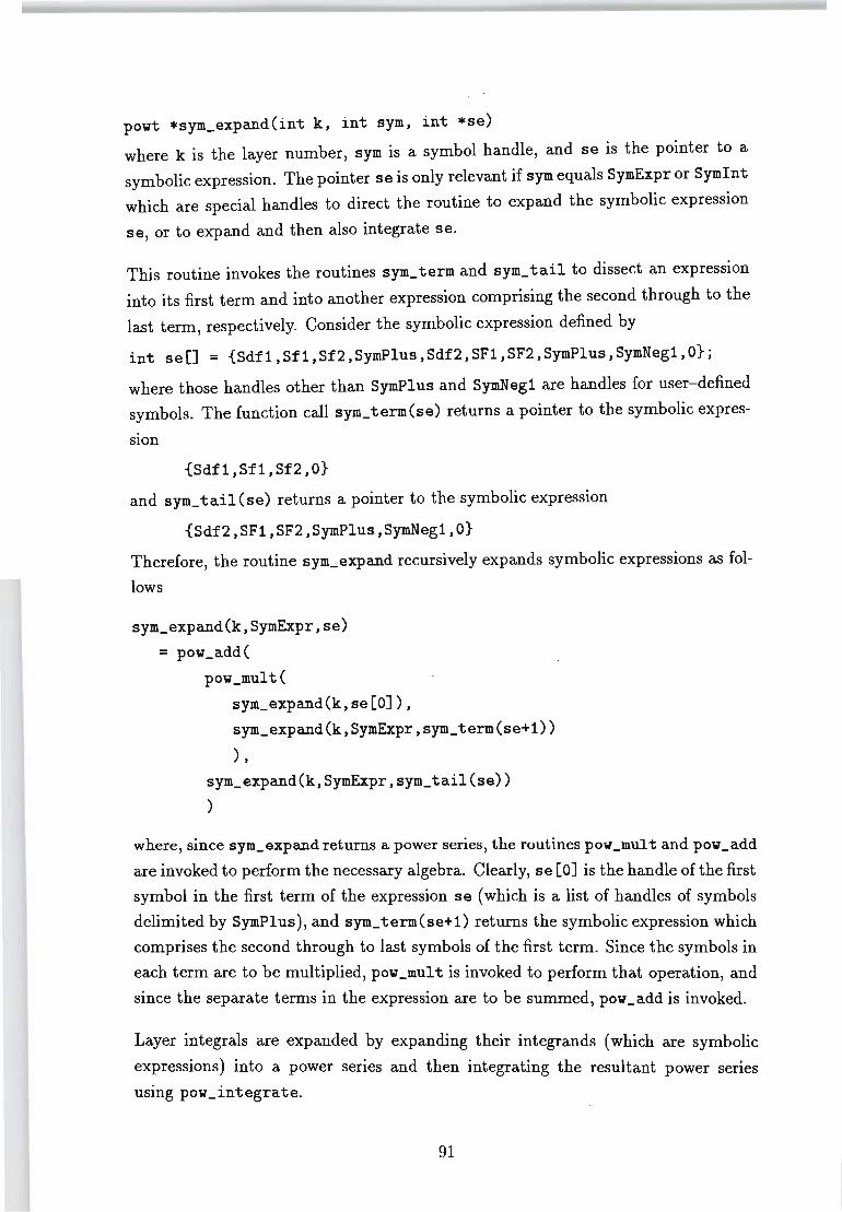
powt *sym_expand(int k, int sym, int *se)
where k is the layer number, sym is a symbol handle, and se is the pointer to a
symbolic expression. The pointer se is only relevant if sym equals SymExpr or Symlnt
which are special handles to direct the routine to expand the symbolic expression
se, or to expand and then also integrate se.
This routine invokes the routines sym_ term and sym_ tail to dissect an expression
into its first term and into another expression comprising the second through to the
last term, respectively. Consider the symbolic expression defined by
int see] = {Sdfl,Sfl,Sf2,SymPlus,Sdf2,SF1,SF2,SymPlus,SymNegl,O};
where those handles other than SymPlus and SymNegl are handles for user-defined
symbols. The function call sym_term(se) returns a pointer to the symbolic expres-
slon
{Sdfl,Sfl,Sf2,O}
and sym_ tail(se) returns a pointer to the symbolic expression
{Sdf2,SF1,SF2,SymPlus,SymNegl,0}
Therefore, the routine sym_expand recursively expands symbolic expressions as fol
lows
sym_expand(k,SymExpr,se)
= pow_add(
pow_mult(
sym_expand(k,se[O]),
sym_expand(k,SymExpr,sym_term(se+l))
) , sym_expand(k,SymExpr,sym_tail(se))
)
where, since sym_expand returns a power series, the routines pow_mul t and pow_add
are invoked to perform the necessary algebra. Clearly, se [0] is the handle of the first
symbol in the first term of the expression se (which is a list of handles of symbols
delimited by SymPlus), and sym_term(se+l) returns the symbolic expression which
comprises the second through to last symbols of the first term. Since the symbols in
each term are to be multiplied, pow _mul t is invoked to perform that operation, and
since the separate terms in the expression are to be summed, pow_add is invoked.
Layer integrals are expanded by expanding their integrands (which are symbolic
expressions) into a power series and then integrating the resultant power series
using pow_integrate.
91

The routine lam_int integrates symbolic expressions from a lower to an upper limit,
and is declared as
real lam_int(int m, int k, int *se)
where se is a pointer to the symbolic expression to be integrated by the operator
The routine sym_expand expands a layer integral from am to z where am ~ ak-l ~
z ~ ak, as follows
sym_expand(k,SymInt,se)
= pow_integrate(sym_expand(k,SymExpr,se),a[k-l],
lam_int(m,k-l,se))
where a[k-l] = ak-l , and m is the index of the lower limit of the layer integral.
When z < am, the algorithm switches to
sym_expand(k,SymInt,se)
= pow_integrate(sym_expand(k,SymExpr,se),a[k],
lam_int(m,k,se))
The routine sym_deri ve invokes sym_expand to expand symbols of the types STExpr
and STInt into power series for each k = 1,2, . . . , n, and stores the n power series
associated with the symbol in the element pp of the symt structure. Symbols which
are definite integrals, i.e. symbols of the type STDInt, evaluate to constants, so
sym_derive evaluates these symbols using lam_int (which invokes sym_expand)
and stores the result in the element rv.
In an application, if a symbol is contained in many symbolic expressions and is itself
a symbolic expression (or an integral of a symbolic expression), the computational
efficiency is improved by deriving that symbol using sym_deri ve before processing
so that the symbol is expanded once only.
4.5.4 Application to Higher-Order Theory
In the application of the special purpose symbolic computation to the higher-order
theory, the symbols relating to the distribution functions given in eqns. (4.18) are defined as follows:
92
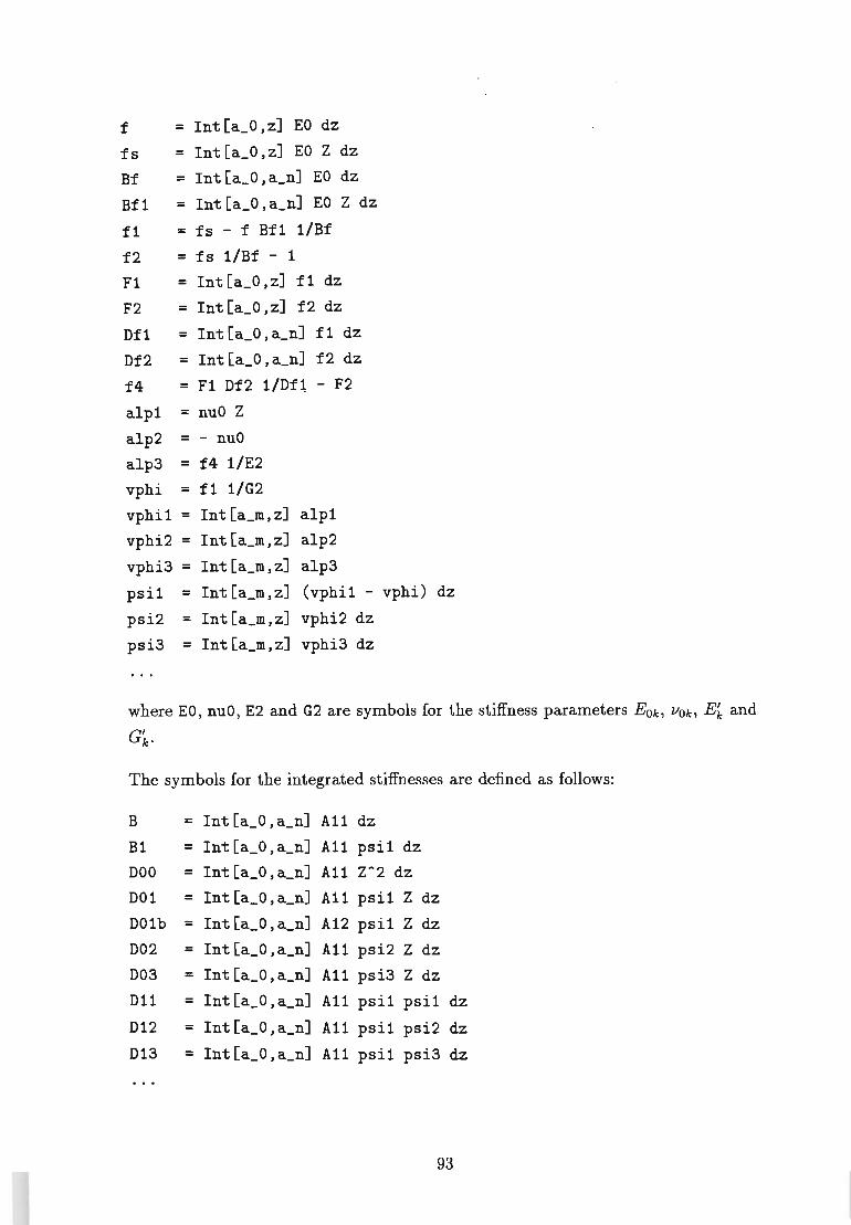
f = Int[a_O,z] EO dz
fs = Int[a_O,z] EO 2 dz
Bf = Int[a_O,a_n] EO dz
Bfl = Int[a_O,a_n] EO 2 dz
fl = fs - f Bfl l/Bf
f2 = fs l/Bf - 1
Fl = Int [a_O ,z] fl dz
F2 = Int[a_O,z] f2 dz
Ofl = Int[a_O,a_n] fl dz
Of2 = Int[a_O,a_n] f2 dz
f4 = Fl Of2 1/0fl - F2
alpl = nuO 2
alp2 = - nuO
alp3 = f4 1/E2
vphi = fl 1/G2
vphil = Int [a_m,z] alpl
vphi2 = Int [a_m,z] alp2
vphi3 = Int [a_m,z] alp3
psil = Int [a_m,z] (vphil - vphi) dz
psi2 = Int [a_m,z] vphi2 dz
psi3 = Int [a_m,z] vphi3 dz
where EO, nuO, E2 and G2 are symbols for the stiffness parameters EOk, lIOk, Ek and
Gk"
The symbols for the integrated stiffnesses are defined as follows:
B = Int [a_O, a_n] A11 dz
Bl = Int [a_O ,a_n] A11 psil dz
DOO = Int [a_O, a_n] A11 2-2 dz
DOl = Int [a_O, a_n] A11 psil 2 dz
DOlb = Int [a_O, a_n] A12 psi1 2 dz D02 = Int [a_O, a_n] A11 psi2 2 dz D03 = Int [a_O, a_n] All psi3 2 dz D11 = Int [a_O ,a_n] A11 psil psil dz
012 = Int [a_O ,a_n] A11 psil psi2 dz 013 = Int [a_O ,a_n] All psi1 psi3 dz
93
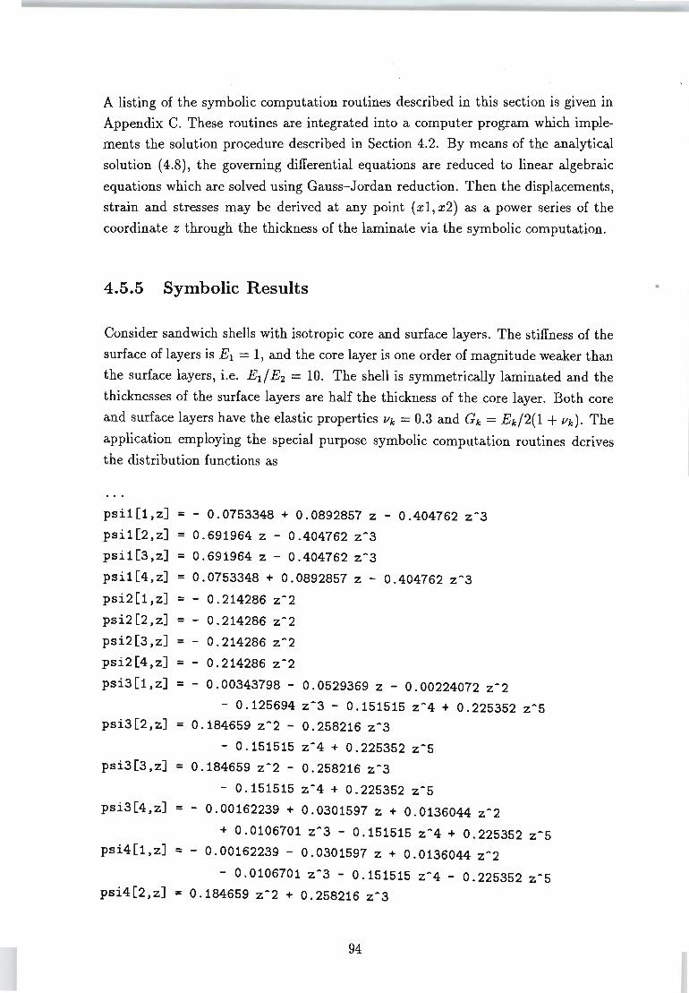
A listing of the symbolic computation routines described in this section is given in
Appendix C. These routines are integrated into a computer program which imple
ments the solution procedure described in Section 4.2. By means of the analytical
solution (4.8), the governing differential equations are reduced to linear algebraic
equations which are solved using Gauss-Jordan reduction. Then the displacements,
strain and stresses may be derived at any point (xl, x2) as a power series of the
coordinate z through the thickness of the laminate via the symbolic computation.
4.5.5 Symbolic Results
Consider sandwich shells with isotropic core and surface layers. The stiffness of the
surface of layers is El = 1, and the core layer is one order of magnitude weaker than
the surface layers, i.e. Ed E2 = 10. The shell is symmetrically laminated and the
thicknesses of the surface layers are half the thickness of the core layer. Both core
and surface layers have the elastic properties Ilk = 0.3 and Gk = Ek /2(1 + Ilk)' The
application employing the special purpose symbolic computation routines derives
the distribution functions as
psi1[1,z] = - 0.0753348 + 0.0892857 z - 0.404762 z-3
psi1[2,z] = 0.691964 z - 0.404762 z-3
psi1[3,z] = 0.691964 z - 0.404762 z-3
psi1[4,z] = 0.0753348 + 0.0892857 z 0.404762 z-3
psi2[1,z] = - 0.214286 z-2
psi2[2,z] = - 0.214286 z-2
psi2[3,z] = - 0.214286 z-2
psi2[4,z] = - 0.214286 z-2
psi3[1,z] = - 0.00343798 - 0.0529369 z - 0.00224072 z-2
- 0.125694 z-3 - 0.151515 z-4 + 0.225352 z-5 psi3[2,z] = 0.184659 z-2 - 0.258216 z-3
- 0.151515 z-4 + 0.225352 z-5
psi3[3,z] = 0.184659 z-2 - 0.258216 z-3
- 0.151515 z-4 + 0.225352 z-5
psi3[4,z] = - 0.00162239 + 0.0301597 z + 0.0136044 z-2
+ 0.0106701 z-3 - 0.151515 z-4 + 0.225352 z-5
psi4[1,z] = - 0.00162239 - 0.0301597 z + 0.0136044 z-2
- 0.0106701 z-3 - 0.151515 z-4 - 0.225352 z-5
psi4[2,z] = 0.184659 z-2 + 0.258216 z-3
94
•
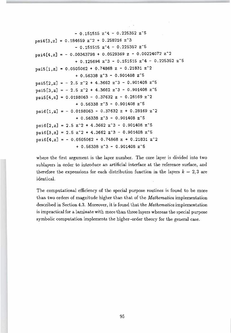
- 0.151515 z-4 - 0.225352 z-5
psi4[3,z] = 0.184659 z-2 + 0.258216 z-3 - 0.151515 z-4 - 0.225352 z-5
psi4[4,z] = - 0.00343798 + 0.0529369 z - 0.00224072 z-2
+ 0.125694 z-3 - 0.151515 z-4 - 0.225352 z-5
psi5[1,z] = 0.0505062 + 0.74868 z - 0.21831 z-2
+ 0.56338 z-3 - 0.901408 z-5
psi5[2,z] = - 2.5 z-2 + 4.3662 z-3 - 0.901408 z-5
psi5[3,z] = - 2.5 z-2 + 4.3662 z-3 - 0.901408 z-5
psi5[4,z] = 0.0198063 - 0.37632 z - 0.28169 z-2
+ 0.56338 z-3 - 0.901408 z-5
psi6[1,z] = - 0.0198063 - 0.37632 z + 0.28169 z-2
+ 0.56338 z-3 - 0.901408 z-5
psi6[2,z] = 2.5 z-2 + 4.3662 z-3 - 0.901408 z-5
psi6[3,z] = 2.5 z-2 + 4.3662 z-3 - 0.901408 z-5
psi6[4,z] = - 0.0505062 + 0.74868 z + 0.21831 z-2
+ 0.56338 z-3 - 0.901408 z-5
where the first argument is the layer number. The core layer is divided into two
sublayers in order to introduce an artificial interface at the reference surface, and
therefore the expressions for each distribution function in the layers k = 2,3 are
identical.
The computational efficiency of the special purpose routines is found to · be more
than two orders of magnitude higher than that of the Mathematica implementation
described in Section 4.3. Moreover, it is found that the Mathematica implementation
is impractical for a laminate with more than three layers whereas the special purpose
symbolic computation implements the higher-order theory for the general case.
95
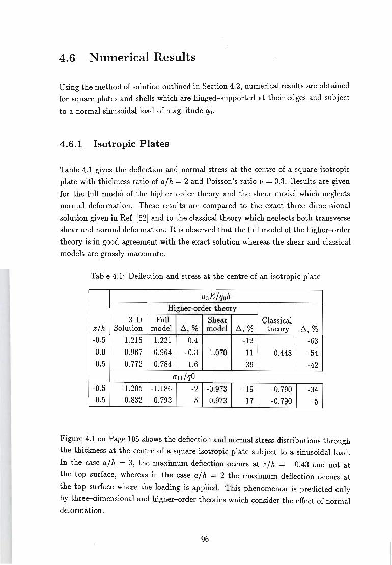
4.6 Numerical Results
Using the method of solution outlined in Section 4.2, numerical results are obtained
for square plates and shells which are hinged-supported at their edges and subject
to a normal sinusoidal load of magnitude qo·
4.6.1 Isotropic Plates
Table 4.1 gives the deflection and normal stress at the centre of a square isotropic
plate with thickness ratio of ajh = 2 and Poisson's ratio v = 0.3. Results are given
for the full model of the higher-order theory and the shear model which neglects
normal deformation. These results are compared to the exact three-dimensional
solution given in Ref. [52] and to the classical theory which neglects both transverse
shear and normal deformation. It is observed that the full model of the higher-order
theory is in good agreement with the exact solution whereas the shear and classical
models are grossly inaccurate.
Table 4.1: Deflection and stress at the centre of an isotropic plate
U3E jqoh Higher-order theory
3-D Full Shear Classical zjh Solution model ~,% model ~,% theory ~,%
-0.5 1.215 1.221 0.4 -12 -63
0.0 0.967 0.964 -0.3 1.070 11 0.448 -54
0.5 0.772 0.784 1.6 39 -42
(jlljqO
-0.5 -1.205 -1.186 -2 -0.973 -19 -0.790 -34 0.5 0.832 0.793 -5 0.973 17 -0.790 -5
Figure 4.1 on Page 105 shows the deflection and normal stress distributions through
the thickness at the centre of a square isotropic plate subject to a sinusoidal load.
In the case ajh = 3, the maximum deflection occurs at zjh = -0.43 and not at
the top surface, whereas in the case ajh = 2 the maximum deflection occurs at
the top surface where the loading is applied. This phenomenon is predicted only
by three-dimensional and higher-order theories which consider the effect of normal deformation.
96

4.6.2 Transversely Isotropic Plates
Table 4.2 gives the deflection and normal stress at the centre of square transversely
isotropic plates with thickness ratio ajh = 5. ' In the case of the shear and classical
models, the modulus E' is equated to 00 and is therefore irrelevant. It is observed
that the effect of normal deformation is substantial in transversely isotropic plates
and this effect increases with E j E'. The shear and classical models which neglect
normal deformation are inaccurate.
Table 4.2: Deflections and normal stresses at the centre of square transversely
isotropic plates (Xl = X2 = aj2) with ajh = 5, v' = 0 and G' = G.
U3E jqoh
Higher-order theory
zjh Shear Classical
Full model model model
EjE' = 1 EjE' = 50 EjE' = 100 EjE' = 1 ... 100
-0.5 21.83 40.01 58.56
-0.25 21.59 28.19 34.93
0 21.42 19.70 17.19 21.46 17.52 0.25 21.34 15.69 9.93 0.5 21.33 15.01 8.56
unjqO
-0.5 -5.15 -6.60 -8.08 -5.12 -4.94 -0.25 -2.39 -2.10 -1.82 -2.39 -2.47 0 -0.01 0.59 1.17 0.00 0.00 0.25 2.38 2.40 2.41 2.39 2.47 0.5 5.11 4.25 3.38 5.12 4.94
Table 4.3 compares the deflection behaviour of isotropic and transversely isotropic
square plates of various thickness ratios. As the thickness ratio of the plate increases,
the effect of normal deformation decreases and the shear model (which predicts a uni
form deflection through the thickness) becomes more accurate. In the transversely
isotropic case (E j E' = 10) where the plate is 10 times weaker in the transverse
direction, the effect of normal deformation is more pronounced, as expected.
Figure 4.2 shows the deflection and normal stress distributions through the thickness
at the centre of a square transversely isotropic plate with ajh = 3, v = 0.3 and
97
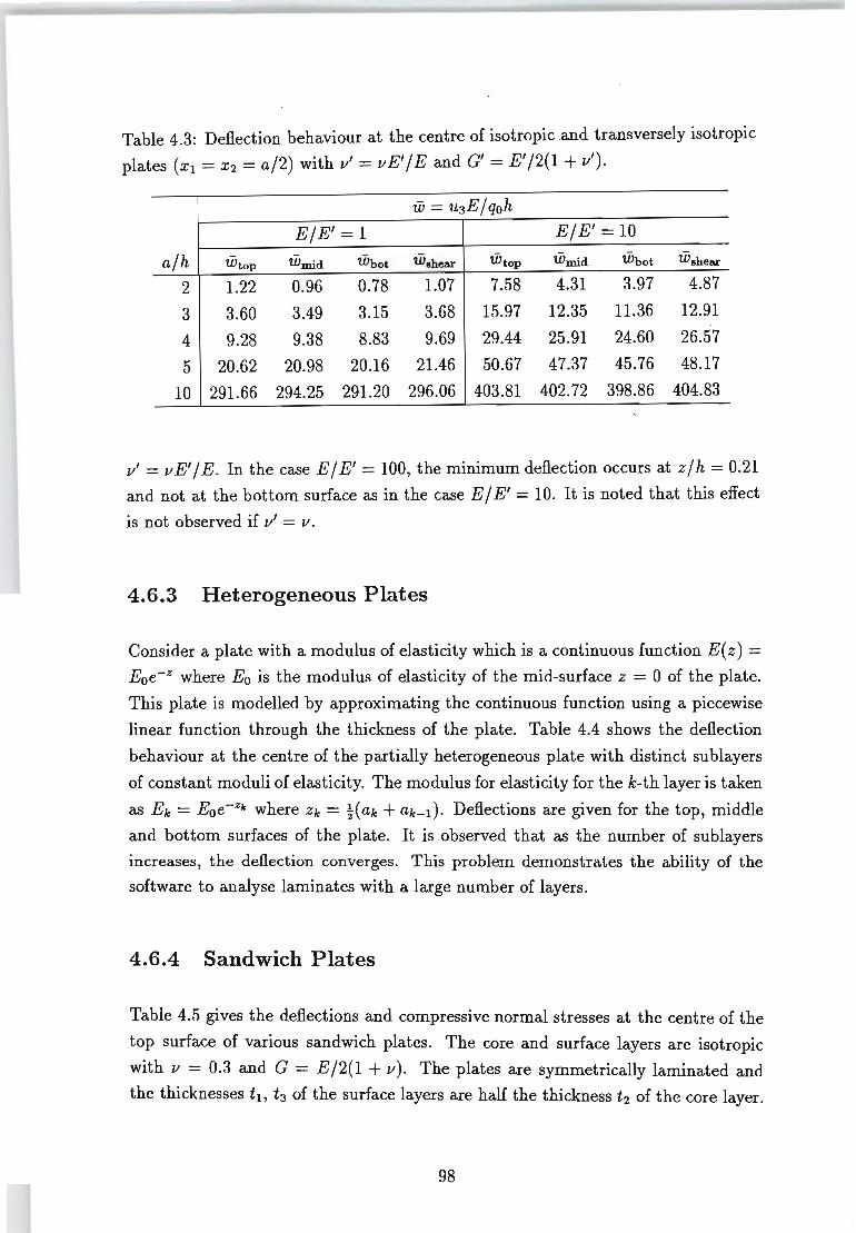
Table 4.3: Deflection behaviour at the centre of isotropic and transversely isotropic
plates (Xl = X2 = a/2) with v' = vE' 1 E and G' = E' /2(1 + v').
W = u3EIQoh EIE' = 1 EIE' = 10
alh Wtop Wmid Whot Wshear Wtop Wmid Whot Wshear
2 1.22 0.96 0.78 1.07 7.58 4.31 3.97 4.87
3 3.60 3.49 3.15 3.68 15.97 12.35 11.36 12.91 4 9.28 9.38 8.83 9.69 29.44 25.91 24.60 26.57 5 20.62 20.98 20.16 21.46 50.67 47.37 45.76 48.17
10 291.66 294.25 291.20 296.06 403.81 402.72 398.86 404.83
v' = v E' 1 E. In the case E 1 E' = 100, the minimum deflection occurs at z 1 h = 0.21
and not at the bottom surface as in the case E 1 E' = 10. It is noted that this effect is not observed if v' = v.
4.6.3 Heterogeneous Plates
Consider a plate with a modulus of elasticity which is a continuous function E(z) =
Eoe-z where Eo is the modulus of elasticity of the mid-surface z = 0 of the plate.
This plate is modelled by approximating the continuous function using a piecewise
linear function through the thickness of the plate. Table 4.4 shows the deflection
behaviour at the centre of the partially heterogeneous plate with distinct sublayers
of constant moduli of elasticity. The modulus for elasticity for the k-th layer is taken
as Ek = Eoe- zlc where Zk = H ak + ak-l). Deflections are given for the top, middle
and bottom surfaces of the plate. It is .observed that as the number of sublayers
increases, the deflection converges. This problem demonstrates the ability of the software to analyse laminates with a large number of layers.
4.6.4 Sandwich Plates
Table 4.5 gives the deflections and compressive normal stresses at the centre of the
top surface of various sandwich plates. The core and surface layers are isotropic
with v = 0.3 and G = E12(1 + v). The plates are symmetrically laminated and
the thicknesses tt, t3 of the surface layers are half the thickness t2 of the core layer.
98
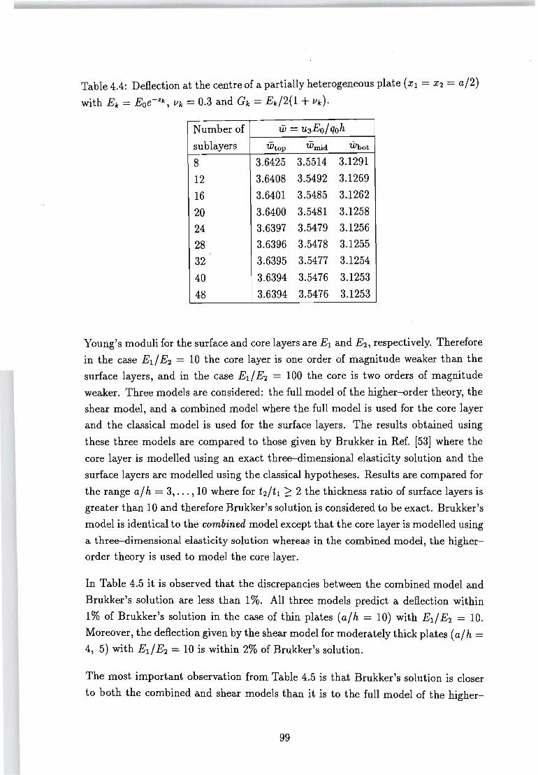
Table 4.4: Deflection at the centre of a partially heterogeneous plate (Xl = X2 = a/2)
with Ek = Eoe-z/c, Vk = 0.3 and Gk = Ek/2(1 + Vk).
Number of W ="U3EO/qoh
sublayers Wtop Wmid Whot
8 3.6425 3.5514 3.1291
12 3.6408 3.5492 3.1269
16 3.6401 3.5485 3.1262
20 3.6400 3.5481 3.1258
24 3.6397 3.5479 3.1256
28 3.6396 3.5478 3.1255
32 3.6395 3.5477 3.1254
40 3.6394 3.5476 3.1253
48 3.6394 3.5476 3.1253
Young's moduli for the surface and core layers are EI and E2, respectively. Therefore
in the case Ed E2 = 10 the core layer is one order of magnitude weaker than the
surface layers, and in the case EI/ E2 = 100 the core is two orders of magnitude
weaker. Three models are considered: the full model of the higher-order theory, the
shear model, and a combined model where the full model is used for the core layer
and the classical model is used for the surface layers. The results obtained using
these three models are compared to those given by Brukker in Ref. [53] where the
core layer is modelled using an exact three-dimensional elasticity solution and the
surface layers are modelled using the classical hypotheses. Results are compared for
the range a/h = 3, ... ,10 where for t2/t l ~ 2 the thickness ratio of surface layers is
greater than 10 and therefore Brukker's solution is considered to be exact. Brukker's
model is identical to the combined model except that the core layer is modelled using
a three-dimensional elasticity solution whereas in the combined model, the higher
order theory is used to model the core layer.
In Table 4.5 it is observed that the discrepancies between the combined model and
Brukker's solution are less than 1%. All three models predict a deflection within
1% of Brukker's solution in the case of thin plates (a/h = 10) with EI/E2 = 10.
Moreover, the deflection given by the shear model for moderately thick plates (a / h = 4, 5) with Ed E2 = 10 is within 2% of Brukker's solution.
The most important observation from Table 4.5 is that Brukker's solution is closer
to both the combined and shear models than it is to the full model of the higher-
99
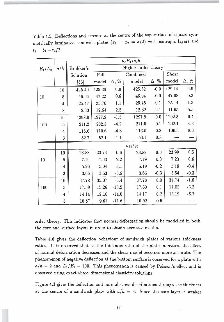
Table 4.5: Deflections and stresses at the centre of the top surface of square sym
metrically laminated sandwich plates (Xl = X2 = a/2) with isotropic layers and
tl = t3 = t 2/2.
u3Edqoh
EI/E2 a/h Brukker's Higher-order theory
Solution Full Combined Shear
[53] model ~,% model ~,% model ~,%
10 425.40 425.36 -0.0 425.32 -0.0 429.14 0.9
10 5 46.96 47.22 0.6 46.94 -0.0 47.08 0.3
4 25.47 25.76 1.1 25.45 -0.1 25.14 -1.3
3 12.33 12.64 2.5 12.32 -0.1 11.65 -5.5
10 1298.0 1277.9 -1.5 1297.9 -0.0 1292.3 -0.4 100 5 211.2 202.3 -4.2 211.5 0.1 202.1 -4.3
4 115.6 110.6 -4.3 116.0 0.3 106.3 -8.0 3 52.7 52.1 -1.1 53.1 0.8 - -
Ull/qO 10 23.88 23.73 -0.6 23.89 0.0 23.99 0.5
10 5 7.19 7.03 -2.2 7.19 0.0 7.23 0.6 4 5.20 5.04 -3.1 5.19 -0.2 5.18 -0.4 3 3.66 3.53 -3.6 3.65 -0.3 3.54 -0.3
10 37.78 35.07 -5.4 37.78 0.0 37.74 -1.8 100 5 17.59 15.26 -13.2 17.60 0.1 17.02 -3.2
4 14.14 12.16 -14.0 14.17 0.2 13.19 -6.7 3 10.87 9.61 -11.6 10.92 0.5 - -
order theory. This indicates that normal deformation should be modelled in both the core and surface layers in order to obtain accurate results.
Table 4.6 gives the deflection behaviour of sandwich plates of various thickness
ratios. It is observed that as the thickness ratio of the plate increases, the effect
of normal deformation decreases and the shear model becomes more accurate. The
phenomenon of negative deflection at the bottom surface is observed for a plate with
a/ h = 2 and Ed E2 = 100. This phenomenon is caused by Poisson's effect and is observed using exact three-dimensional elasticity solutions.
Figure 4.3 gives the deflection and normal stress distributions through the thickness
at the centre of a sandwich plate with a/ h = 3. Since the core layer is weaker
100
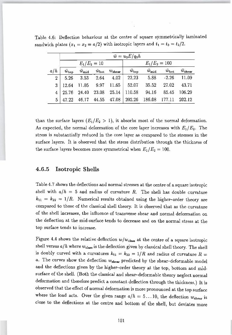
Table 4.6: Deflection behaviour at the centre of square symmetrically laminated
sandwich plates (Xl = X2 = a/2) with isotropic layers and tl = t3 = t 2/2.
W = U3E/Qoh
El/E2 = 10 El/E2 = 100
a/h Wtop Wmid Wbot Wshear Wtop Wmid Wbot Wshear
2 5.26 3.53 2.64 4.02 22.23 5.88 -2.26 11.09
3 12.64 11.05 9.97 11.65 52.07 35.52 27.02 43.71
4 25.76 24.40 23.08 25.14 110.58 94.16 85.45 106.29
5 47.22 46.17 44.55 47.08 202.26 186.08 177.11 202.12
than the surface layers (Ed E2 > 1), it absorbs most of the normal deformation.
As expected, the normal deformation of the core layer increases with El / E2 • The
stress is substantially reduced in the core layer as compared to the stresses in the
surface layers. It is observed that the stress distribution through the thickness of
the surface layers becomes more symmetrical when Ed E2 = 100.
4.6.5 Isotropic Shells
Table 4.7 shows the deflections and normal stresses at the centre of a square isotropic
shell with a/h = 5 and radius of curvature R. The shell has double curvature
kll = k22 = 1/ R. Numerical results obtained using the higher-order theory are
compared to those of the classical shell theory. It is observed that as the curvature
of the shell increases, the influence of transverse shear and normal deformation on
the deflection at the mid-surface tends to decrease and on the normal stress at the top surface tends to increase.
Figure 4.4 shows the relative deflection W / Wclass at the centre of a square isotropic
shell versus a / h where Wclass is the deflection given by classical shell theory. The shell
is doubly curved with a curvatures kll = k22 = 1/ R and radius of curvature R =
a. The curves show the deflection Wshear predicted by the shear-deformable model
and the deflections given by the higher-order theory at the top, bottom and mid
surface of the shell. (Both the classical and shear-deformable theory neglect normal
deformation and therefore predict a constant deflection through the thickness.) It is
observed that the effect of normal deformation is more pronounced at the top surface
where the load acts. Over the given range a/ h = 5 ... 10, the deflection Wshear is
close to the deflections at the centre and bottom of the shell, but deviates more
101
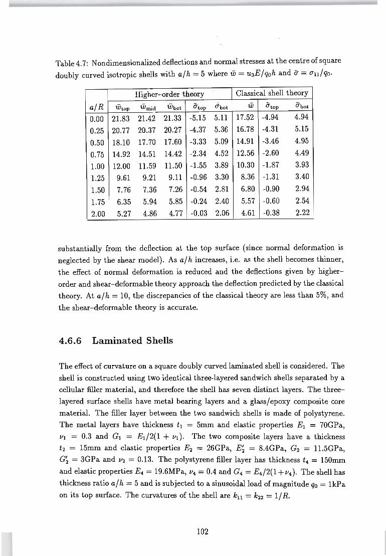
Table 4.7: N ondimensionalized deflections and normal stresses at the centre of square
doubly curved isotropic shells with a/h = 5 where W = U3E/qoh and ij = un/qo.
Higher-order theory Classical shell theory
aiR Wtop Wmid Wbot Utop Ubot W Utop Ubot
0.00 21.83 21.42 21.33 -5.15 5.11 17.52 -4.94 4.94
0.25 20.77 20.37 20.27 -4.37 5.36 16.78 -4.31 5.15
0.50 18.10 17.70 17.60 -3.33 5.09 14.91 -3.46 4.95
0.75 14.92 14.51 14.42 -2.34 4.52 12.56 -2.60 4.49
1.00 12.00 11.59 11.50 -1.55 3.89 10.30 -1.87 3.93
1.25 9.61 9.21 9.11 -0.96 3.30 8.36 -1.31 3.40
1.50 7.76 7.36 7.26 -0.54 2.81 6.80 -0.90 2.94
1.75 6.35 5.94 5.85 -0.24 2.40 5.57 -0.60 2.54
2.00 5.27 4.86 4.77 -0.03 2.06 4.61 -0.38 2.22
substantially from the deflection at the top surface (since normal deformation is
neglected by the shear model). As a/h increases, i.e. as the shell becomes thinner,
the effect of normal deformation is reduced and the deflections given by higher
order and shear-deformable theory approach the deflection predicted by the classical
theory. At a/h = 10, the discrepancies of the classical theory are less than 5%, and
the shear-deformable theory is accurate.
4.6.6 Laminated Shells
The effect of curvature on a square doubly curved laminated shell is considered. The
shell is constructed using two identical three-layered sandwich shells separated by a
cellular filler material, and therefore the shell has seven distinct layers. The three
layered surface shells have metal bearing layers and a glass/epoxy composite core
material. The filler layer between the two sandwich shells is made of polystyrene.
The metal layers have thickness tl = 5mm and elastic properties El = 70GPa,
111 = 0.3 and Gl = Ed2(1 + 111)' The two composite layers have a thickness
t2 = 15mm and elastic properties E2 = 26GPa, E~ = 8.4GPa, G2 = 11.5GPa,
G~ = 3GPa and 112 = 0.13. The polystyrene filler layer has thickness t4 = 150mm
and elastic properties E4 = 19.6MPa, 114 = 0.4 and G4 = E4/2(1 + 114). The shell has
thickness ratio a/ h = 5 and is subjected to a sinusoidal load of magnitude qo = 1kPa
on its top surface. The curvatures of the shell are kll = k22 = 1/ R.
102
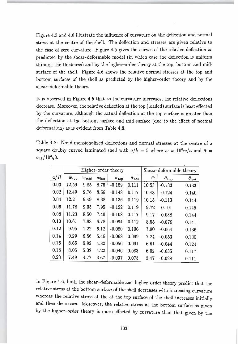
Figure 4.5 and 4.6 illustrate the influence of curvature on the deflection and normal
stress at the centre of the shell. The deflection and stresses are given relative to
the case of zero curvature. Figure 4.5 gives the curves of the relative deflection as
predicted by the shear-deformable model (in which case the deflection is uniform
through the thickness) and by the higher--order theory at the top, bottom and mid
surface of the shell. Figure 4.6 shows the relative normal stresses at the top and
bottom surfaces of the shell as predicted by the higher--order theory and by the
shear-deformable theory.
It is observed in Figure 4.5 that as the curvature increases, the relative deflections
decrease. Moreover, the relative deflection at the top (loaded) surface is least effected
by the curvature, although the actual deflection at the top surface is greater than
the deflection at the bottom surface and mid-surface (due to the effect of normal
deformation) as is evident from Table 4.8.
Table 4.8: Nondimensionalized deflections and normal stresses at the centre of a
square doubly curved laminated shell with a/h = 5 where W = 106w/a and a = 0"1l/103 qO.
Higher--order theory Shear-deformable theory
aiR Wtop Wmid Wbot atop abot W atop O"bot
0.00 12.59 9.85 8.75 -0.159 0.111 10.53 -0.133 0.133
0.02 12.49 9.76 8.66 -0.148 0.117 10.43 -0.124 0.140
0.04 12.21 9.49 8.38 -0.136 0.119 10.15 -0.113 0.144
0.06 11.78 9.05 7.95 -0.122 0.119 9.72 -0.101 0.145 0.08 11.23 8.50 7.40 -0.108 0.117 9.17 -0.088 0.144 0.10 10.61 7.88 6.78 -0.094 0.112 8.55 -0.076 0.141 0.12 9.95 7.22 6.12 -0.080 0.106 7.90 -0.064 0.136 0.14 9.29 6.56 5.46 -0.068 0.099 7.24 -0.053 0.130 0.16 8.65 5.92 4.82 -0.056 0.091 6.61 -0.044 0.124 0.18 8.05 5.32 4.22 -0.046 0.083 6.02 -0.035 0.117 ,
0.20 7.49 4.77 3.67 -0.037 0.075 5.47 -0.028 0.111
In Figure 4.6, both the shear-deformable and higher--order theory predict that the
relative stress at the bottom surface of the shell decreases with increasing curvature
whereas the relative stress at the at the top surface of the shell increases initially
and then decreases. Moreover, the relative stress at the bottom surface as given
by the higher--order theory is more effected by curvature than that given by the
103

shear-deformable theory, whereas the relative stress at the top surface given by the
two theories are similarly effected by curvature.
104
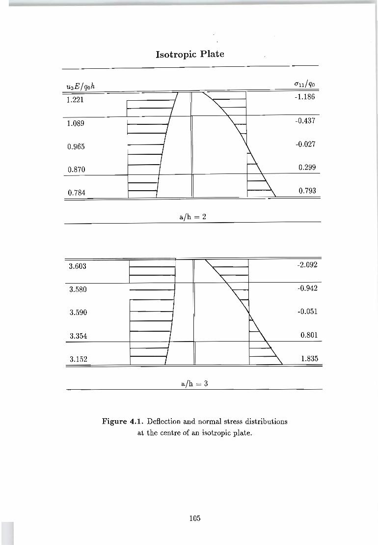
1.221
1.089
0.965
0.870
0.784
3.603
3.580
3.590
3.354
3.152
Isotropic Plate
j " j "-I " J \ I
] J
~ I
\ \
1 \
a/h = 2
"' " '\. ~
I ~ J \. J \. I \.
a/h = 3
Figure 4.1. Deflection and normal stress distributions
at the centre of an isotropic plate.
105
-1.186
-0.437
-0.027
0.299
0.793
-2.092
-0.942
-0.051
0.801
1.835
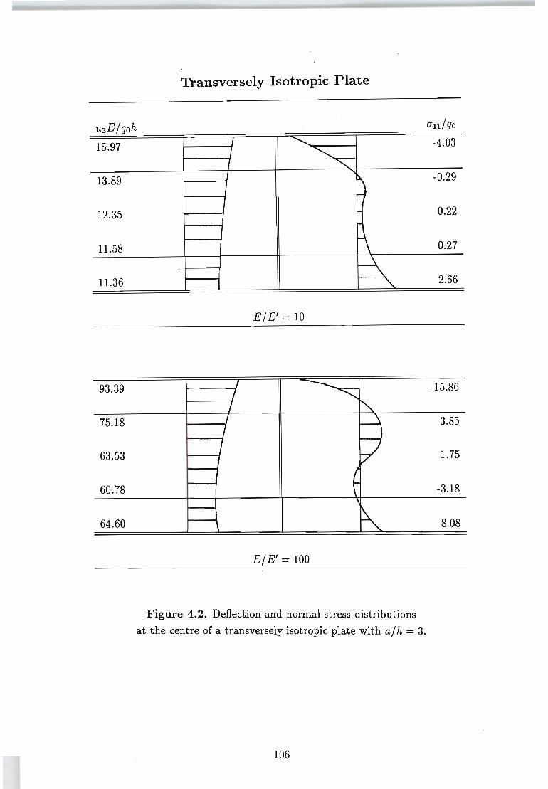
Transversely Isotropic Plate
u E/qoh 3
15.97
13.89
12.35
11.58
11.36
93.39
75.18
63.53
60.78
64.60
7 ............. I ~ I
I
~ ~
~ ~
'\..
E/E' = 10
7 ---7
""'"" I '" I
~ / I
J
{
~ E/E' = 100
Figure 4.2. Deflection and normal stress distributions
at the centre of a transversely isotropic plate with a/ h = 3.
106
-4.03
-0.29
0.22
0.27
2.66
-15.86
3.85
1.75
-3.18
8.08

12.64
12.62
11.04
10.16
9.97
57.07
51.97
35.52
27.07
27.02
Sandwich Plate
-~ ~
I
~
--t::::::...
I ~
~
Figure 4.3. Deflection and normal stress distributions at the
centre of a sandwich plate with a/h = 3, t2 /t 1 = 2
and isotropic core and surface layers.
107
-3.53
0.74
-0.21
-0.13
-0.09
-0.33
3.06
9.61
8.32
-0.22
-0.14
-0.11
-4.13
5.20
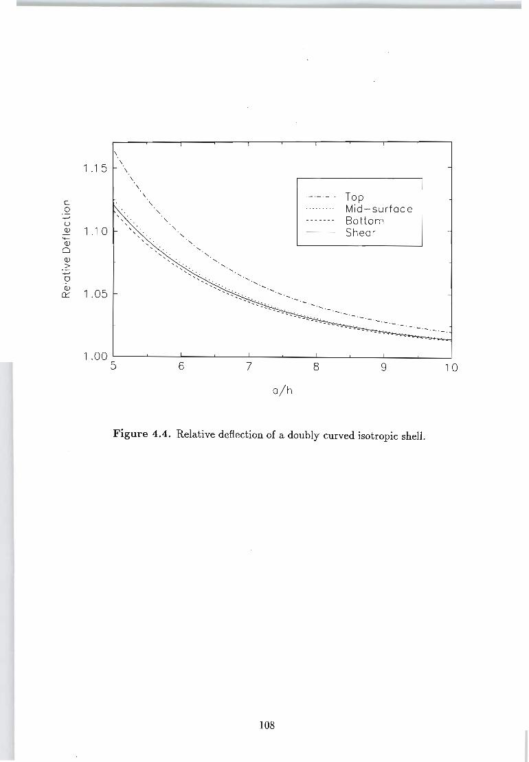
C 0 +J <.) Q)
'+--Q)
0 Q)
> +J
0 Q)
0:::
\
\
1 .1 5 \
\
\
\
, , , 1 .1 0
, , , , ,
1 .05
\
" "-"-
, , , , , , ,
"-"-
"-"-
"-, "-
"-
Top Mid - surfac e Botto m Shear
-- .-
1 .00 L-__ ~ ____ -L ____ ~ ____ ~ __ ~ ____ ~ ____ ~ ____ ~ __ ~ ____ ~
5 6 7 8 9 10
a/h
Figure 4.4. Relative deflection of a doubly curved isotropic shell.
108
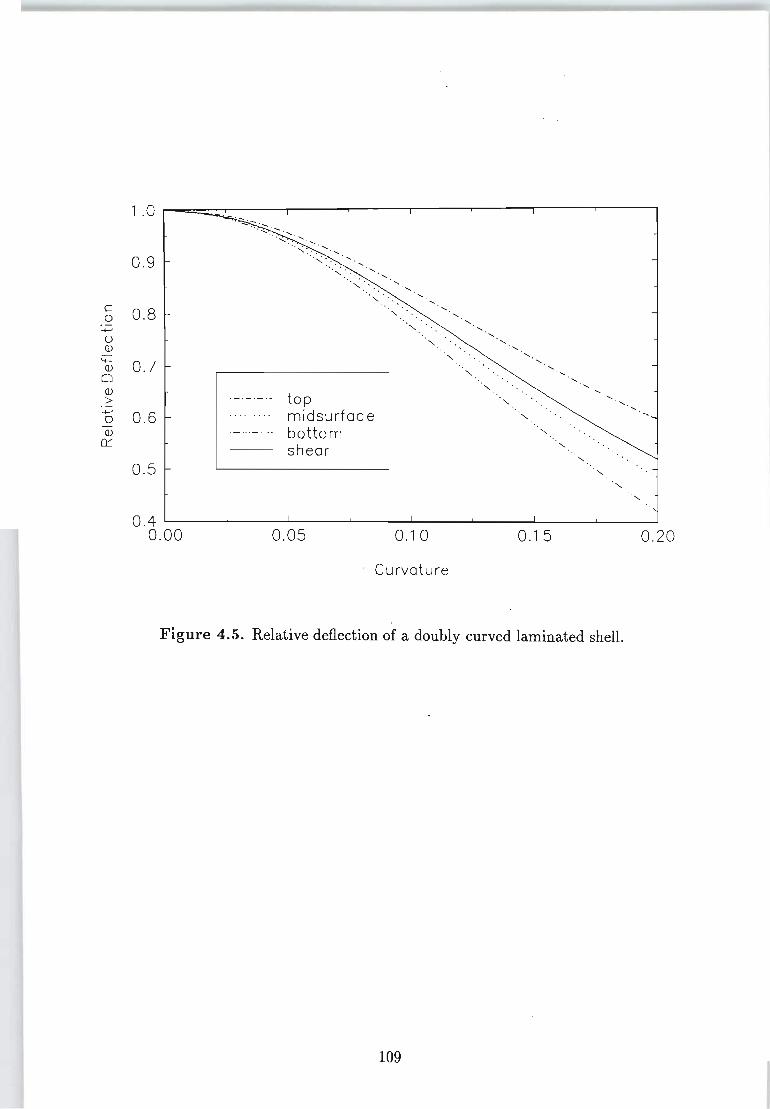
c 0
+-'
0 OJ
"'-OJ
0 OJ > ......, 0 OJ
0:::
1 .0
0 .9
0.8
0.7
0 .6
0 .5
0.4 0.00
, '.
top midsurface bottom shear
0 .05
, '.
" ".
"'". .......
'. ".
0 .1 0
Curvature
0.15
Figure 4.5. Relative deflection of a doubly curved laminated shell.
109
0 .20
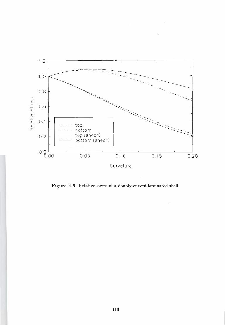
(j) (j) Q) L. .....,
(f)
Q)
> ....., 0 Q)
n::::
1 .2
1 .0
0.8
0 .6
0.4
0.2
top bottom top (shear) bottom (shear)
-. -.
0.0 ~----~----~----~----~------~----~----~----~ 0 .00 0.05 0 .10 0 .15 0.20
Curvature
Figure 4.6. Relative stress of a doubly curved laminated shell.
110
4.7 Conclusions
The comprehensive higher-order theory presented in Chapter 3 is implemented for
computational studies. In the general case, the distribution functions and integrated
stiffnesses cannot be derived in a form suitable for direct numerical implementation,
and the calculation of these functions using a numerical method detracts from the
increased accuracy offered by the higher-order theory. Therefore symbolic com
putation is employed to derive the distribution functions, calculate the integrated
stiffness constants, solve the system of governing differential equations analytically,
and finally to evaluate the stress/strain state of a given laminate.
The theory is implemented using the Mathematica symbolic computation system,
and this application is used to derive analytical results and obtain numerical results.
However, in order to improve the computational efficiency of the analysis, special
purpose symbolic computation routines are developed in the C programming lan
guage as an alternative to using a general purpose symbolic computation system such
as Mathematica. The routines handle symbolic expressions where the symbols may
be defined as piecewise integrals through thickness of a laminate, laminae stiffness
parameters, constants or symbolic expressions. Symbols and symbolic expressions
are expanded into power series using a recursion technique. It is found that the
special purpose symbolic computation is more than two orders of magnitude more
efficient than Mathematica owing to its dedication to the requirements of the specific
problem .
.The numerical results obtained for thick homogeneous and heterogeneous plates are
compared to those in the literature in order to validate the hig~er-order theory. It
is found that for an isotropic plate with thickness ratio a/h = 2, the higher-order
theory predicts the deflection distribution to within 2%, and the normal stresses
to within 5%, of the exact three-dimensional elasticity solution, whereas the shear
deformable model (which neglects the effect of normal deformation) and the classical model are grossly inaccurate.
The more weaker plates are in the transverse direction, the more pronounced is the
effect of normal deformation, and the inaccuracy of the shear~deformable model
increases. However, it is observed that as the ratio a/ h increases, i.e. the structure
becomes thinner, the effect of normal deformation is reduced, and for plates with
a/h 2:: 10, i.e. thin plates, the shear-deformable theory may be considered to be accurate.
111

Numerical results are given for doubly curved isotropic shells. with thickness ratio
a/h = 5. It is observed that as the curvature of the shell increases, the influence of
transverse shear and normaf deformation on the deflection at the mid-surface tends
to decrease and on the normal stress at the loaded surface tends to increase.
Numerical results for sandwich plates where the higher-order theory is used to model
the core layer and the classical theory is used to model the surface layers are com
pared to those given in the literature where the core layer is modelled as a three
dimensional elastic body. It is found that the discrepancies are at most 0.8% over
the range a/ h = 3, ... ,10 for the core layer one or two orders of magnitude weaker
than the surface layers.
The higher-order theory predicts phenomena which can only be observed using
three-dimensional elasticity solutions or a theory which considers normal deforma
tion. In particular, in the case of an isotropic plate with a/h = 3, the maximum
deflection occurs near the top surface where the loading is applied, whereas in the
case a/h = 2 the maximum deflection occurs at the top surface. Moreover, for a
sandwich plate with a/h = 2, negative deflection is observed at the bottom surface
when the core layer is two orders of magnitude weaker than the surface layers, but
is not observed when the core layer is only one order weaker than the surface layers.
It is noted that this phenomenon is caused by Poisson's effect.
The numerical results obtained indicate that the new higher-order theory is accu
rate for thick structures, whereas, in general, the shear-deformable theory and the
classical theory are inaccurate. Therefore in the analysis of thick structures, not
only transverse shear but also normal deformation should be taken into account.
112
Chapter 5
Optimization of Thick Sandwich
Plates based on Higher-Order
Theory
5 .1 Introduction
The objective of the present chapter is the optimization of thick sandwich structures
on the basis of the higher-order theory presented in Chapter 3.
In the case of sandwich plates with significantly different mechanical properties of the
surface and core layers, normal deformation needs to be accounted for to determine
the deflection profile through the thickness in an accurate manner. The core layer
absorbs some of the deformation and this leads to vastly different deflections of the
top and bottom surfaces of the plate with the amount of core deformation depending
on the relative stiffnesses and thicknesses of the surface and core layers. Moreover
the stress distribution through the thickness of thick laminated plates is no longer
symmetrical even for symmetrical structures. This is due to the fact that the load is
applied on the top surface and it is physically clear that due to the non-symmetry
of loading, the resulting stress distribution cannot be symmetrical as predicted by
theories which fail to take normal deformation into account.
It is known that the classical theory yields inaccurate results for thick composite
structures as a result of neglecting transverse shear and normal deformation. Since
the accurate analysis of the stress and strain behaviour of thick laminated compos
ite plates is essential for the optimal design of such structures, the classical theory
113
cannot be used for this purpose. Moreover, it is shown in this chapter that shear
deformable theories (which neglect normal deformation) are also inadequate for the
design optimization of thick plates. Clearly a three-dimensional elasticity solution
would provide an accurate analysis. However, such solutions are computationally
demanding. Therefore, owing to the importance of both accuracy and computa
tional efficiency in design optimization studies, the higher-order theory developed
in Chapter 3 is better suited to such studies. Certainly the accuracy of this theory
was demonstrated in the previous chapter, and, as discussed in Sections 3.1 and 3.2,
the computational demands of single-layer theories such as this higher-order theory,
are less than those of three-dimensional and discrete-layer higher-order theories.
However, the computational implementation of the proposed higher-order theory
poses special computational problems due to the need to evaluate multiple piecewise
integrals through the thickness of the laminate to compute stiffnesses. Moreover,
due to the iterative nature of optimization solutions, these calculations need to be
performed using computationally efficient algorithms. These difficulties are over
come by developing special purpose symbolic computation routines to perform the
necessary calculations. The routines developed in this chapter bypass some of the
symbolic processing performed by the more flexible routines developed in Section 4.5
in order to improve the efficiency of the symbolic computations.
Three optimal design problems for thick laminated sandwich plates are considered.
The first problem involves the minimum weight design of a sandwich plate subject to
a constraint on the deflection of the bottom surface. The design variables are chosen
as the thickness of the core layer and the fibre content of the surface layers which
are made of a transversely isotropic composite material. Numerical results are given
for a sandwich plate with a steel honeycomb core layer. The relationship between
the laminate thickness, fibre content and deflection constraint is established.
The second problem involves the minimum deflection design of a sandwich plate.
In this problem the relative thickness of the surface and core layers is chosen as
the design variable. The optimal design for minimum deflection is based on the
observation that the deflection of the bottom surface decreases as the core thickness
becomes smaller, but increases again once this thickness drops below a certain level.
Moreover, the bottom surface may undergo negative deflection for certain combina
tions of material properties. These phenomena are peculiar to thick structures and
can only be analysed using three-dimensional elasticity solutions or a higher-order
theory which includes normal deformation. The effect of the relative stiffness of the
surface and core layers on the optimal thickness of the surface layers is investigated.
114
The third problem is a minimum stress problem which involves the computation of
the relative thicknesses of the layers such that the resulting lamination will reflect
the stress pattern in a more realistic fashion and thereby will minimize the maximum
stress. In this regard, the present study departs from conventional designs which
automatically assume a symmetrical lamination. In the case of thick structures,
such conventional designs cease to be optimal as shown in this chapter.
5.2 Literature survey
A number of refined theories were developed for sandwich plates to include the effect
of shear deformation in the surface and core layers [67, 68, 69]. However optimum
designs of sandwich plates and shells were mostly based on classical sandwich the
ory. Various optimization studies for sandwich structures include minimum weight
beams [70], plates under compressive loads [71, 72] and bending loads [73], and
acoustic sandwich panels [74]. Design of sandwich shells with fibre composite sur
face layers was given in Refs. [75] and [76]. Sandwich plates under uncertain bending
loads were designed in Ref. [77] .
The design of thick sandwich structures does not seem to be studied using a higher
order theory which includes normal as well as shear deformation. In fact previous
studies on the optimal design of thick laminated structures seem to be based on
shear-deformable theories only. In this regard, studies include maximum frequency
design [78, 79], maximum buckling load design [79, 80], and maximum stiffness design [81].
5.3 Software
In this section, software dedicated to the implementation of the higher-<>rder theory
for design optimization is developed in the C programming language.
This software processes power series and double trigonometric series using simple
programming techniques. The routines which handle power series are used for
the calculation of the distribution functions and integrated stiffness constants of
the higher-<>rder theory, and the routines which handle trigonometric series are
used for the calculation of the displacements (3.37) and (3.38), strains (3.40) and stresses (3.42) using the solution (4.8) of the system (4.6).
115
The special purpose symbolic computation routines developed in this chapter for the
derivation of the distribution functions and calculation of the integrated stiffnesses
differ from the more flexible but less efficient routines developed in Section 4.5. The
routines developed in the present study mimic the symbolic computations of those of
Section 4.5 but without the recursive expansion of symbolic expressions. Rather, the
various operations to derive symbols (such as the distribution functions) as power
series or to evaluate symbols (such as the integrated stiffness) are explicitly initiated
via calls to routines which perform those operations. For example, if the next step of
the procedure is to sum two particular symbols, the relevant operator routine, in this
case a routine which handles summation, is called with arguments which reference
the two operands. In Section 4.5, a symbolic expression could be defined and the
operator routines would be initiated automatically with the appropriate arguments
by the routine which expands a symbolic expression into a power series.
5.3.1 Symbols
In the application, the distribution functions tPgk, CPqk, f3tk and fr.qk in eqns. (3.37),
(3.38) and (3.40) become symbols which are referred to by handles. For example,
the function tPlk is referenced by the handle Fpsil, an enumerated constant. These
symbols are n vectors of power series with a maximum of Pc coefficients. The
coefficients of these symbols are stored in a multidimensional array and the handles
to the symbols are used as indices to the first dimension of the array. The index
to the second dimension is the layer number k, and the third dimension contains
the Pc coefficients of the power series of the relevant symbol for the k-th layer. In
the application, the value of a symbol is returned by the C function zfn (sym, k, z)
where sym is the handle of the symbol to be evaluated at z where ak-l =:; z < ak.
5.3.2 Distribution Functions
First a set of routines is developed for the derivation of the distribution functions.
This set includes routines for algebraic operations involving power series. Also, the
routine calc_layint performs the layer integral operations (4.16) and (4.17) using the observation that
(5.1)
116
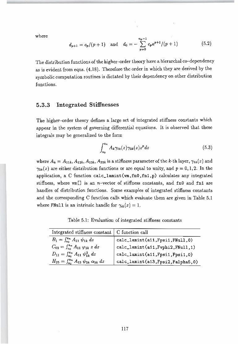
where np-l
dp+1 = Cp/(p + 1) and do = - I: CpaP+1 /(p + 1) (5.2)
p=O
The distribution functions of the higher-order theory have a hierarchal co-dependency
as is evident from eqns. (4.18). Therefore the order in which they are derived by the
symbolic computation routines is dictated by their dependency on other distribution
functions.
5.3.3 Integrated Stiffnesses
The higher-order theory defines a large set of integrated stiffness constants which
appear in the system of governing differential equations. It is observed that these
integrals may be generalized to the form
(5.3)
where Ak = AUk, A12k , A l3k , A33k is a stiffness parameter of the k-th layer, /'lk(z) and
/'2k(Z) are either distribution functions or are equal to unity, and p = 0,1,2. In the
application, a C function calc_lamint (vm, fnO, fnl, p) calculates any integrated
stiffness, where vm [] is an n-vector of stiffness constants, and fnO and fnl are
handles of distribution functions. Some examples of integrated stiffness constants
and the corresponding C function calls which evaluate them are given in Table 5.1
where FNull is an intrinsic handle for /'ik(Z) = 1.
Table 5.1: Evaluation of integrated stiffness constants
Integrated stiffness constant
Bl = f:on Au "plk dz
CO2 = f:on Au 'P2k Z dz
Du = f:on Au "pik dz
H2S = f:n Al3 "p2k aSk dz
C function call
calc_lamint(all,Fpsil,FNull,O)
calc_lamint(all,Fvphi2,FNull,1)
calc_lamint(all,Fpsil,Fpsil,O)
calc_lamint(a13,Fpsi2~Falpha5,O)
117
5.3.4 Trigonometric Series
The second set of routines is dedicated to processing trigonometric series approxi
mations of the functions
U;(X), W(X), Xg(X) (i=1,2; 9=1, ... ,8) (5.4)
which are required for the calculation of the displacements, stresses and strains.
In the application, these series are symbols referred to by a handle which is an
enumerated constant.
The coefficients of the solution (4.8) of the system (4.6) are solved for any given pair
(m, n) using Gauss-Jordan reduction, and the coefficients of X3(X), ... , Xs(x) are
determined from the given loading. These coefficients are then stored in an array
which is indexed by the handle of the symbol.
The routine eval_ trig_ term differentiates and evaluates a term of the form
(5.5)
A routine eval_ trig takes the handle of a symbol as an argument, and uses eval_
trig_ term to differentiate and evaluate a double trigonometric series whose terms
are of the form (5.5) and whose coefficients have been calculated.
Macro symbols for the trigonometric approximations of the functions (5.4) are de
fined; for example the C directives
#define xul(xl,x2,td)
#define xw(xl,x2,td)
#define xchil(xl,x2,td)
eval_trig( Cul,
eval_trig( Cw,
Tcos_sin,td,xl,x2)
Tsin_sin,td,xl,x2)
eval_trig( Cchil, Tsin_sin,td,xl,x2)
define macros for the symbols for the functions Ul(X), w(x) and Xl(X), where Cul,
Cw and Cchi 1 are their handles and td indicates the differential operation to be
performed. For example W,12(Xl, X2) is evaluated by the macro xw(xl ,x2, TD12) as
given in Table 5.2.
Using these macros, the displacements (3.37), deflection (3.38), strains (3.40) and
stresses (3.42) are readily evaluated.
The entire analysis based on the higher-order theory is incorporated into an opti
mization algorithm where, in each iteration, the stress/strain state of the plate is
determined from the configuration and material properties and of the laminate.
118
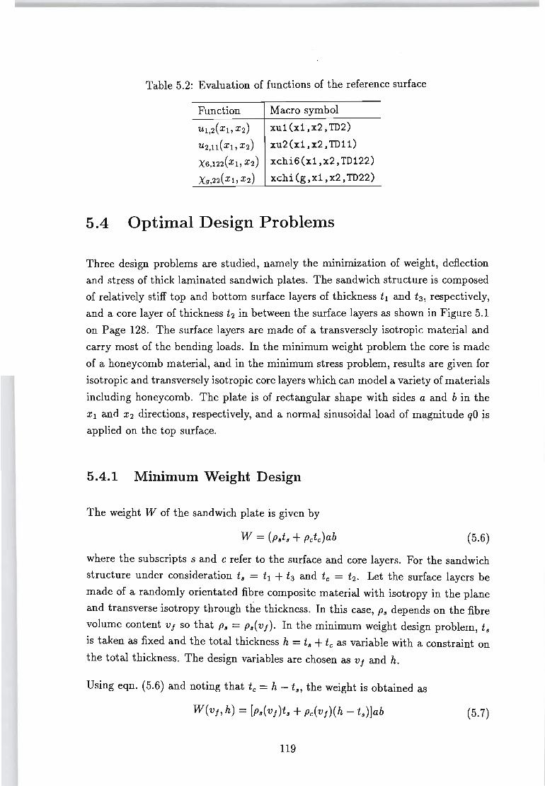
Table 5.2: Evaluation of functions of the reference surface
Function Macro symbol
Ul,2(XbX2) xu1(x1.x2.TD2)
U2,n(XbX2) xu2(x1.x2.TD11)
X6,l22(Xb X2) xchi6 (x1.x2. TD122)
X9,22(Xb X2) xchi(g.x1.x2. TD22)
5.4 Optimal Design Problems
Three design problems are studied, namely the minimization of weight, deflection
and stress of thick laminated sandwich plates. The sandwich structure is composed
of relatively stiff top and bottom surface layers of thickness tl and t 3, respectively,
and a core layer of thickness t2 in between the surface layers as shown in Figure 5.1
on Page 128. The surface layers are made of a transversely isotropic material and
carry most of the bending loads. In the minimum weight problem the core is made
of a honeycomb material, and in the minimum stress problem, results are given for
isotropic and transversely isotropic core layers which can model a variety of materials
including honeycomb. The plate is of rectangular shape with sides a and b in the
Xl and X2 directions , respectively, and a normal sinusoidal load of magnitude qO is
applied on the top surface.
5.4.1 Minimum Weight Design
The weight W of the sandwich plate is given by
(5.6)
where the subscripts sand c refer to the surface and core layers. For the sandwich
structure under consideration tlJ = tl + t3 and tc = t 2. Let the surface layers be
made of a randomly orientated fibre composite material with isotropy in the plane
and transverse isotropy through the thickness. In this case, PIJ depends on the fibre
volume content Vj so that PIJ = plJ(Vj). In the minimum weight design problem, tlJ
is taken as fixed and the total thickness h = tlJ + tc as variable with a constraint on
the total thickness. The design variables are chosen as vJ and h.
Using eqn. (5.6) and noting that tc = h - t lJ , the weight is obtained as
(5.7)
119
The design problem can be stated as
(5.8)
subject to thickness and fibre content constraints
h ~ ho, Vf,min ~ vf ~ vf,max (5.9)
and a deflection constraint at a given point
(5.10)
where ho, Vf,min, vJ,max and Wo are specified quantities and Wb denotes the deflection
of the bottom surface. As the higher-order theory employed in this study is capable
of determining the deflection at any point through the thickness of the plate, the
location of the deflection in the z-direction has to be specified for design purposes.
The deflection of the bottom surface is chosen as a constraint because of its practical
importance.
The deflection depends on the fibre content v f through the values of the elastic
constants E6 , E~, G6 , G~ and 1I1J. For an in-plane randomly oriented material, the
following micromechanical equations are used
EIJ EJvJ/3 + Emvm
E' 6 E'm/(l - (1- 3E'm/Ej).jVf)
G6 Gf vJl3 + GmVm
G' 6 Gm /(l - (1 - 3Gm/Gj )Vf)
116 0.3 (5.11)
where f and m refer to the fibre and matrix properties, respectively, and a prime
indicates a property in the transverse direction.
Here the expressions EIJ and G6 are taken from Ref. [82] and the factor 1/3 reflects
the reduction in moduli for a randomly oriented fibre composite as compared to
a unidirectional composite. The expressions are valid for sufficiently stiff fibres
(Ef » Em) [82]. The expressions for E~ and G~ for the elastic constants through
the thickness are taken from Ref. [83] and the fibre properties are multiplied by a
factor 1/3 in line with the expressions for E6 and G6 to account for the random
orientation of the fibres. An average value is assigned to 116 [82].
The density is computed from
(5.12)
120
The efficiency of a minimum weight design can be assessed by defining an efficiency
index given by Wmin
7]= W(0.5,.h)
(5.13)
where W(0.5, h) is the weight of a plate made of surface layers only with vI = 0.5
and h determined such that the deflection constraint (5.10) is satisfied. The index
provides a weight comparison between the optimally designed sandwich structure
and its single layer counterpart with no core region.
The minimum weight design involves the computation of the fibre content v I and
the total thickness h so as to solve the optimization problem (5.8)-(5.10). For a
given h and deflection constraint Wo, the minimum vI is determined such that the
inequality (5.10) is satisfied. The optimal h is obtained by minimising the weight
over h. This procedure yields the minimum weight sandwich having the optimal v I
and h. A Golden Section algorithm is used to compute the minimum fibre content
v I and the optimal thickness hopt '
5.4.2 Minimum Deflection Design
The deflection behaviour of thick sandwich structures differ substantially from their
thin counterparts when the effects of shear and normal deformation are taken into
account and the optimal design problem should be formulated accordingly. One
difference involves the deflection of the bottom surface with the load applied at
the top surface. In this case, as the thickness of the surface layers increase, the
deflection of the bottom surface does not necessarily decrease. In fact it decreases
with increasing tl and t3, but starts to increase after reaching a minimum. This is
observed in Figure 5.2 on Page 129 where the curves of Wb at the centre of the plate
are plotted against t. = tl + t3 with t3 = tl for a square laminate with a/h = 2 and
Ed E2 = 50. In Figure 5.2, Wb is nondimensionalised with respect to the deflection
Wiso of an isotropic plate with stiffness E = E1 • It is observed that the deflection of
the sandwich plate approaches that of the isotropic plate as t. increases.
The deflection behaviour observed in Figure 5.2 can be explained by noting that the
core layer absorbs some of the deformation in the normal direction. However, if the
core layer becomes too thin, its capacity to absorb the deflection diminishes, leading
to an increase in the deflection of the bottom surface as the core thickness becomes
too smalL As a result the bottom surface of a structure with no core layer may
deflect more than an optimally designed sandwich structure. This phenomenon can
121
neither be investigated nor taken into account using the classical theory of plates or
a theory which excludes the effect of normal deformation.
In the light of these results the minimum deflection problem may be stated as
minmaxWb(Xl, X2, t a) t. X1,X2
(5.14)
where 0 :::; ts :::; h with ts = 0 and ts = h corresponding to a plate of core layer
only and surface layer only, respectively. The efficiency of the optimally designed
laminates is assessed by defining the ratio
h = Wb(XI, X2;topt)
Wb(XI,X2; h) (5.15)
where (XI, X2) is the location of maximum deflection, topt the optimal value of ts
and Wb( XI, X2; h) the deflection of a laminate composed of surface layers only. The
quantity h serves as an efficiency index to compare the optimal sandwich to its single
layer counterpart with no core layer.
The solution of the minimum deflection problem is obtained by solving the minmax
problem (5.14) which yields the optimal thickness of the surface layers.
5.4.3 Minimum Stress Design
In thick sandwich plates with a core region whose stiffness is relatively low, the stress
distribution through the thickness is not symmetrical even if the lamination is. This
is due to the fact that the transverse load applied on the top surface leads to stresses
in the top layers which are different from those in the bottom layers. The resulting
stress distribution cannot be symmetrical as predicted by theories which fail to take
normal deformation into account. An optimal design for minimum stress involves
the computation of the relative thicknesses of layers such that the maximum normal
stress will be minimized.
The normal stresses are given by Un = un(XI, X2, z, t1 ) and U22 = U22(XI, X2, z, t1 )
with the core thickness t2 being a given parameter. Then the maximum normal
stress is given by
The optimal design problem can be stated as
mlnumax t1
122
(5.16)
(5.17)
for a given total thickness h = tl + t2 + t3. The thickness of the top and bottom
layers are subject to the practical constraint
(5.18)
In the present problem, the total thickness h is specified and t2 is an input parameter.
Thus t3 = h - tl - t2 where tl is the optimal thickness of the top layer.
5.5 Numerical Results
Numerical results are given for a square sandwich plate of dimensions a x a (a = 1m)
subjected to a sinusoidal load of amplitude qo = 1 MPa on the top surface.
5.5.1 Minimum Weight Design
Results are given for surface layers made of T300 graphite fibres whose properties
are taken as
EI = 258.6 GPa, Ei = 18.2 GPa, vI = 0.2
GI = 36.7 GPa, G, = 20 GPa, PI = 1750kg/m3 (5.19)
and the epoxy matrix properties are taken as
Em = 3.45 GPa, Vm = 0.35
Gm = Em/2(1 + vm), Pm = 1200 kg/m3 (5.20)
The core section is made of a 17-7 PH stainless steel honeycomb material with the
elastic constants [84]
Ec = 1.58 GPa, Pc = 124 kg/m3
(5.21) GXllC = 0.50 GPa, GlIZC = 0.68 GPa
These values correspond to a honeycomb with a cell size of 0.25in. First the depen
dence of the weight Won the thickness h is investigated for various values of t8 and
Wo as shown in Figure 5.3 on Page 130. It is observed that W displays a minimum
point with respect to h which increases with increasing t8. The fibre contents for
various values of t8 and Wo are shown in Figure 5.4 with 0.2 ~ vI ~ 0.7. As expected
VI decreases as h increases for a given t 8 , but increases as the deflection constraint becomes smaller.
123
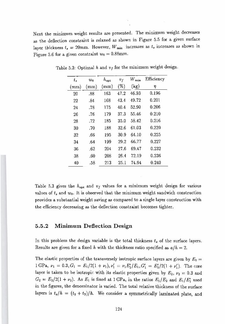
N ext the minimum weight results are presented. The minimum weight decreases
as the deflection constraint is relaxed as shown in Figure 5.5 for a given surface
layer thickness t8 = 20mm. However, W min increases as t8 increases as shown in
Figure 5.6 for a given constraint Wo = 0.88mm.
Table 5.3: Optimal hand Vf for the minimum weight design.
t8 Wo hopt vf W min Efficiency
(mm) (mm) (mm) (%) (kg) 7J
20 .88 163 47.2 46.93 0.196
22 .84 168 43.4 49.72 0.201
24 .78 175 40.4 52.90 0.206
26 .76 179 37.3 55.46 0.210
28 .72 185 35.0 58.42 0.216
30 .70 188 32.6 61.03 0.220
32 .66 195 30.9 64.10 0.225
34 .64 199 29.2 66.77 0.227
36 .62 204 27.6 69.47 0.232
38 .60 208 26.4 72.19 0.236
40 .58 213 25.1 74.94 0.240
Table 5.3 gives the hopt and v f values for a minimum weight design for various
values of t8 and woo It is observed that the minimum weight sandwich construction
provides a substantial weight saving as compared to a single layer construction with
the efficiency decreasing as the deflection constraint becomes tighter.
5.5.2 Minimum Deflection Design
In this problem the design variable is the total thickness t8 of the surface layers.
Results are given for a fixed h with the thickness ratio specified as a/h = 2.
The elastic properties of the transversely isotropic surface layers are given by EI = 1 GPa, VI = 0.3, GI = Ed2(1 + VI)' vf = vlEU Ell G~ = EU2(1 + vD. The core layer is taken to be isotropic with its elastic properties given by E2, V2 = 0.3 and
G2 = E2/2(1 + V2) . As EI is fixed at 1 GPa, in the ratios Ed E2 and Ell Ef used
in the figures, the denominator is varied. The total relative thickness of the surface
layers is t8/h = (tl + t3)/h. We consider a symmetrically laminated plate, and
124
Figure 5.7 shows the optimal thickness topt!h vs Ed E2 for Ed E~ = 5,10,20. It is
observed that topt decreases as the ratio Ell E 2 increases, that is, as the surface layers
become stronger relative to the core layer. The minimum values of the deflection,
Wb,min, are given in Figure 5.8. As Ell E2 increases, Wb,min decreases due to the
core region absorbing more of the normal deformation. An interesting phenomenon
observed in Figure 5.8 is the existence of negative deflection for Ell E~ = 5 when
Ell E2 ~ 74. This phenomenon is further investigated below. Figure 5.9 gives
the corresponding curves for the efficiency ratio b. The efficiency of the design,
in general, increases as Ell E2 increases, i.e., as the core layer becomes weaker.
Negative values for b occur as a result of Wb,min becoming negative for certain ratios
of elastic moduli as observed in Figure 5.8.
Figure 5.10 shows the curves of the toptlh plotted against Ed E~ for various values of
Ed E2. It is observed that topt increases for high values of Ed E2 and decreases for
low values of Ell E2 as Ed E~ increases, i.e., as the through-the-thickness modulus
E~ decreases. For intermediate values, i.e. for Ed E2 = 50, it increases for low
values of Ell E~ and decreases as Ed E~ increases. As shown in Figure 5.11, the
values of Wb,min increase as E~ becomes smaller. The corresponding efficiency curves
are given in Figure 5.12. Again it is observed that b is negative in some cases.
Next the behaviour of the deflection through the thickness. is investigated, in par
ticular the phenomenon of negative deflection and the effect of excluding normal
deformation. Figure 5.13 shows the deflection curves through the thickness of the
plate for various cases with Ed E2 = 50 and Ell E~ = 10. The deflection curve
for the optimal sandwich with topt/ h = 0.803 (tl = t2 = topt/2) is shown in Fig
ure 5.13a. It is observed that the top layer deflects more than the bottom one and
there exists a minimum point across the thickness. The corresponding curve for a
single-layered laminate is shown in Figure 5.13b. For this case the efficiency index
is b = 1.11/3.79 = 0.293 indicating a 70% reduction in the deflection. Figure 5.13c
shows the deflection of the sandwich plate with the effect of normal deformation
neglected. It is clear that neglecting this effect leads to a completely erroneous result.
The corresponding deflection curves are given in Figures 5.14a, 5.14b and 5.14c for
Ed E2 = 90 and Ed E~ = 5. In is observed from Figure 5.14a that the bottom
surface of the optimal sandwich has a negative deflection. This explains the neg
ative values for b which for this case is b = -0.443/1.11 = -0.40. Figure 5.14c
again shows the effect of neglecting the normal deformation. In this case the phe-
125
nomenon of negative deflection cannot be observed when the normal deformation is
left unaccounted.
5.5.3 Minimum Stress Design
The elastic properties of the transversely isotropic surface layers are given by El =
1 GPa, E~ = E1/2, 111 = 1I~ = 0.3, Gl = El/2(1 + lid and G~ = E~/2(1 + 1If). The
elastic properties ofthe core layer are given by E2, 112 = 1I~ = 0.15, G2 = E2/2(1+1I2) and G~ = E~/2(1 + 1I~). As El is fixed at 1 GPa, in the ratio El / E2 used in the
figures, the denominator is varied.
To assess the efficiency of the designs, a comparison is made between the optimally
designed and symmetrical sandwich plates. For this purpose, an efficiency index is
defined as (5.22)
where ti indicates the optimal thickness of the top surface and £1 = (h - t 2 )/2, i.e.
the thickness of the top layer of a symmetrical plate. In the discussion below, 1] is
referred to as the stress ratio.
First the behaviour of the stress ratio is investigated as a function of the design
variable t l . Figure 5.15a shows the curves of 1] versus tl/h for various values of the
core thickness t2/h for a thickness ratio 'of a/h = 2 and an isotropic core layer. It
is observed that in general the minimum stress ratio is achieved by a nonsymmetric
design. Figure 5.15b shows the same curves as in Figure 5.15a with the effect of
normal deformation neglected. For this case, the results indicate that the optimal
design is always a symmetric laminate and the stress ratio is greater than one for
any other configuration. Therefore it is essential to include normal deformation
in the analysis of thick sandwich plates to obtain the correct optimization results.
Figure 5.16a shows the curves of 1] versus tl/h for various thickness ratios for a
transversely isotropic core with E~/ E2 = 10 and t2/h = 0.5. As in the previous
case, the stress ratio in minimized at certain values of t l . Figure 5.16b shows the
same curves as in Figure 5.16a with the effect of normal deformation neglected. In
the vicinity of the optimal point (tl/h = 0.25), the greater the thickness ratio, the
greater the error as compared to the results given in Figure 5.16a. Figures 5.15
and 5.16 indicate that an optimal choice of tl can lead to substantial reductions in
the stress ratio, i.e., the optimal plate will be considerably more efficient than the
symmetrical one as determined by the efficiency index 1].
126
The optimal values of t l , denoted by ti, and the corresponding stress ratios are plot
ted against t2/h in Figure 5.17 for various values of Ed E2. The jump discontinuities
in the values of tl occur due to the existence of local minima. It is observed that
in all cases the top layer is thinner than the bottom layer except for Ed E2 = 10
and t2/h = 0.8. However, ti approaches the symmetrical case as t2 increases. Fig
ure 5.17b shows that the efficiency of the design drops as t2 increases. The curves of
ti/h and 7J versus a/h are shown in Figure 5.18 for various values of t2/h and with
E;/ E2 = 1 (isotropic core). As a/h increases, i.e., as the plate becomes thinner, tUh
tends to get larger, and in some cases, the top layer can be thicker than the bottom
layer. This situation arises as the core layer becomes thicker. As a/h increases, the
efficiency drops, except for the case t2 / h = 0.8 as can be seen from Figure 5.18b.
Corresponding curves for a sandwich plate with a transversely isotropic core are
given in Figure 5.19 where E;/ E2 = 10. In this case, the top layer can be thicker
than the bottom layer in several cases. However, the general trend of ti/h as a
function of a/h is similar to the case with an isotropic core layer. A comparison
of Figures 5.18b and 5.19b indicates that the efficiency drops in the case of a plate
with a transversely isotropic core.
The effect of stiffness ratio Ed E2 on ti and 7J is investigated in Figure 5.20 which
shows the curves of ti/h and 7J versus Ed E2 for a/h = 4. The results are obtained
subject to the constraint tdh ~ 0.02. It is observed that ti shows different trends
depending on the values of t2/h and E I / E2. The efficiency, in general, improves with increasing Ed E2.
Typical stress distributions through the thickness are shown in Figure 5.21 for the
case a/h = 3, Ed E2 = 20, E I / E~ = 2, E;/ E2 = 1 and t2/h = 0.6. Figure 5.21a
shows the stress distribution for an optimal plate, Figure 5.21b for a symmetrical
plate, and Figure 5.21c for a symmetrical plate with the effect of normal deformation
neglected. It is observed that in the case of an optimal plate, the maximum stresses
are the same at the top and bottom layers. Figure 5.21c indicates that neglecting
normal deformation would yield a completely incorrect stress distribution and render
the solution meaningless as is illustrated by Figures 5.15b and 5.16b.
127
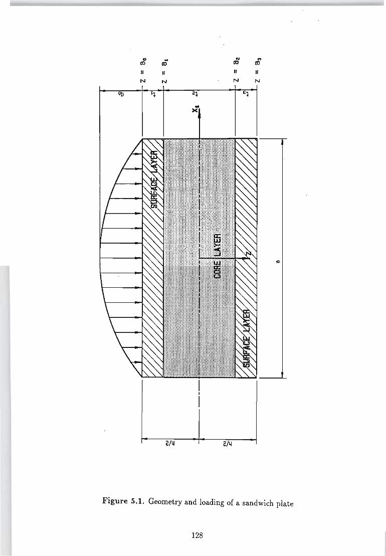
0 N 1'1 ... to to to to II II II II
N N N N
J~ i!~ £~
... ><
2/1l GIll
Figure 5.1. Geometry and loading of a sandwich plate
128
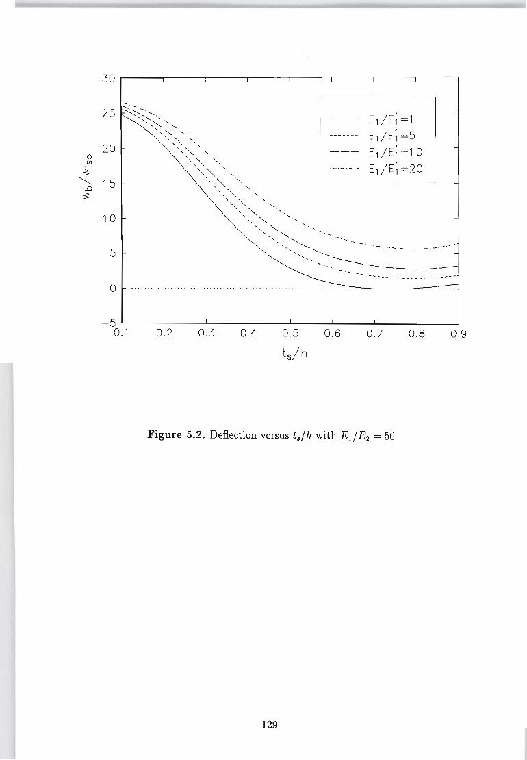
0 UJ
~ ~
..0 3
30
25
20
15
10
5
0
E1/E;=1
E1 IE; =5
E1 IE; =10
E1 I E; =20
--'- - .---_ . - . - .-. - '
--------- -----------------
- .. .. ~ ... . . .. .. -- . . .......... -...... -- . -- .. . .. .. ..... ..... . -- --- .. ~ .. -:-: .. ~. ----~ .. ..,..., .. -:-: .. -:-... . . .
-5 ~----~----~----~----~------~----~----~----~ 0.1 0.2 0.3 0.4 0 .5 0.6 0.7 0.8 0 .9
ts/h
Figure 5.2. Deflection versus til / h with Ed E2 = 50
129
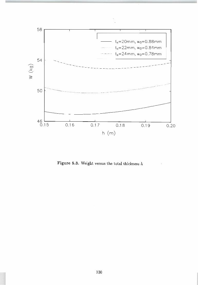
58~------~-------.--------,-----~-,-------.
54
50
-.-"-' "- -- .
t s =20mm, wo=0.88mm
-------------- ts=22mm, wo=0 .84mm
-- -- --.- ts=24mm, wo=0_78mm
.-.-
46 L-________ ~ ________ ~ ________ ~ ________ ~ ______ ~
0 .15 0.1 6 0 .17 0.18 0_19 0.20
h (m)
Figure 5.3. Weight versus the total thickness h
130
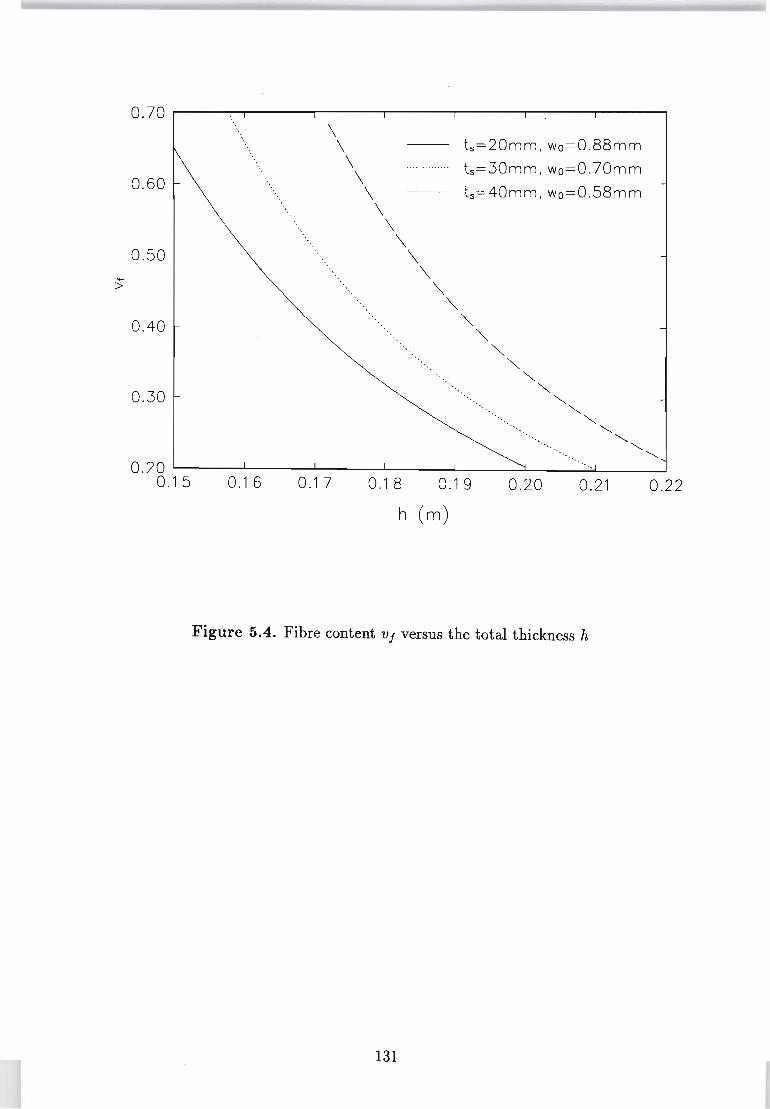
0.70~----~----~----~----~----,-----~----,
ts=20mm, wo=0 .88mm
ts=30mm, wo=0 .70mm 0.60 ts=40mm, wo=0 .58mm
0 .50
0.40
0.30
0 .20 L---......I.....------lL-__ ....L. __ --L ___ :::1..-__ ...:.:..L. __ ---l
0.15 0.1 6 0.1 7 0.18 0 .1 9 0.20 0.21 0.22
h (m)
Figure 5.4. Fibre content vi versus the total thickness h
131
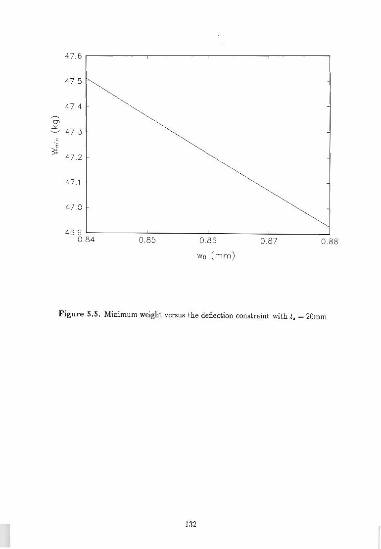
47.6
47. 5
47.4 ,.........."
Q) .:Y
47 .3 '-../
c 'E
3: 47.2
47.1
47 .0
46 .9 0 .84 0.85 0.86 0.87 0 .88
Wo (mm )
Figure 5.5. Minimum weight versus the deflection constraint with ts = 20mm
132
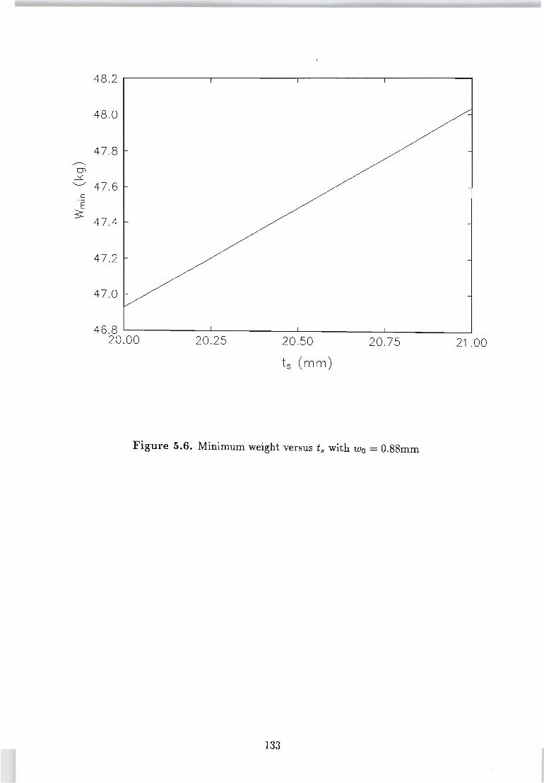
48.2
48.0
47 .8 ....---..
O"l .::s:. '-.../ 47 .6
c
E 3:
47.4
47 .2
47 .0
46 .8 20.00 20.25 20.50 20 .75 21 .00
ts (mm)
Figure 5.6. Minimum weight versus ts with Wo = O.88mm
133
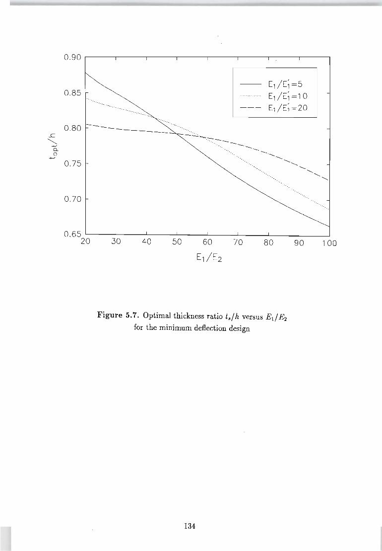
0.90 .---------r---,-------,----,--r---r~--,---__,
0.85
0.80 ----------
0.75
0 .70
-'~'~.-:----." .... '. --- -- --- --.. ---
E1 I E; =5
E1 I E; =1 0
E1 I E; =20
--.................. ......... , ,
"
0.65 ~--~----~----~----~----~----~--~--__ ~ 20 30 40 50 70 80
Figure 5.7. Optimal thickness ratio t,,/h versus EdE2 for the minimum deflection design
134
90 100
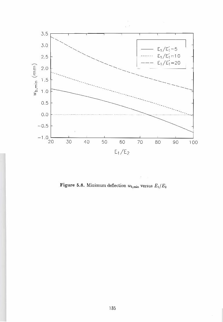
3.5 1 I I I
3.0
2.5 ,,--..,
E 2.0 E
'-../
C 1 .5 E .0 1 .0 ~
0.5
0.0 ................ ................. .... .... ....... ................... .
-0.5
-1 .0 L-__ ~~ __ ~ ____ ~ ____ ~ ____ ~ ____ ~ ____ ~ ____ ~
20 30 40 50 70 80 90 100
Figure 5.8. Minimum deflection Wb,min versus Ed E2
135
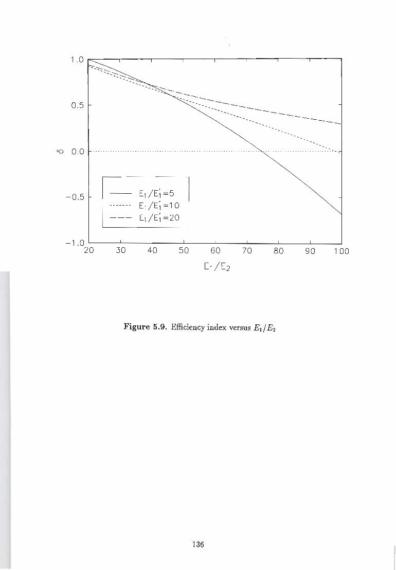
1 .0 ~----~----.-----.-----r-----r-----r-----r-----'
0.5
---..:.----... - --' ......... --...----
... - ~-----------------'0 0 .0 ....... .. .... ... ....... .............. ........... ........... ... ..... .
-0.5 E1/E;=5 ------- E1/E;=10 --- E1 /E; =20
-1.0 20 30 40 50 60 70 80 90 100
E1/E2
Figure 5.9. Efficiency index versus Ed E2
136
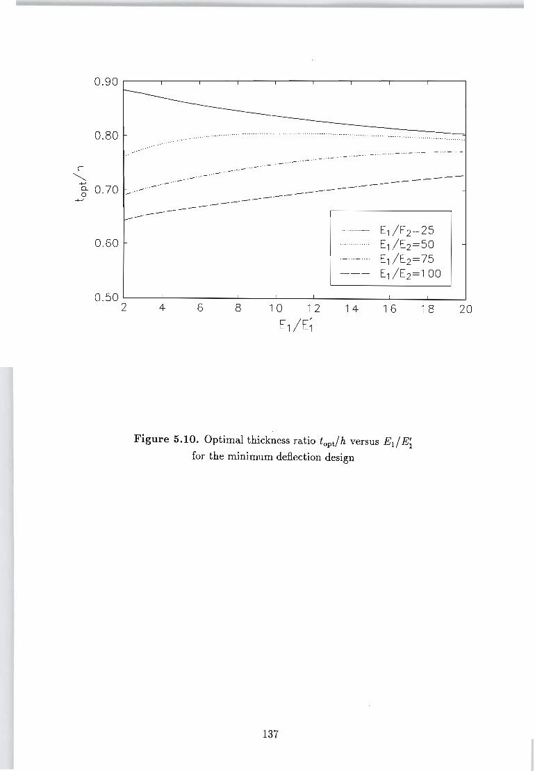
...c ~ ....,
0.90~--.----,----,---,----,---'----.----r--~
.-====--------J 0.80 ................... .................................................................... .
- , .. -.. --
- , .. - ' .- ... -. .. - '.
'- -" ' - "' - " -- .. - -.- - -
---------g- 0.70 ------------ "'-
~----------0.60
----E1/ E2=25 E1/E2=50 E1 / E2=75 E1 /E2=1 00
0.502L----4L---~6~--~8----~10----1~2----1~4----1~6----1~8--~20
E1 I E;
Figure 5.10. Optimal thickness ratio topt! h versus Ed E~ for the minimum deflection design
137
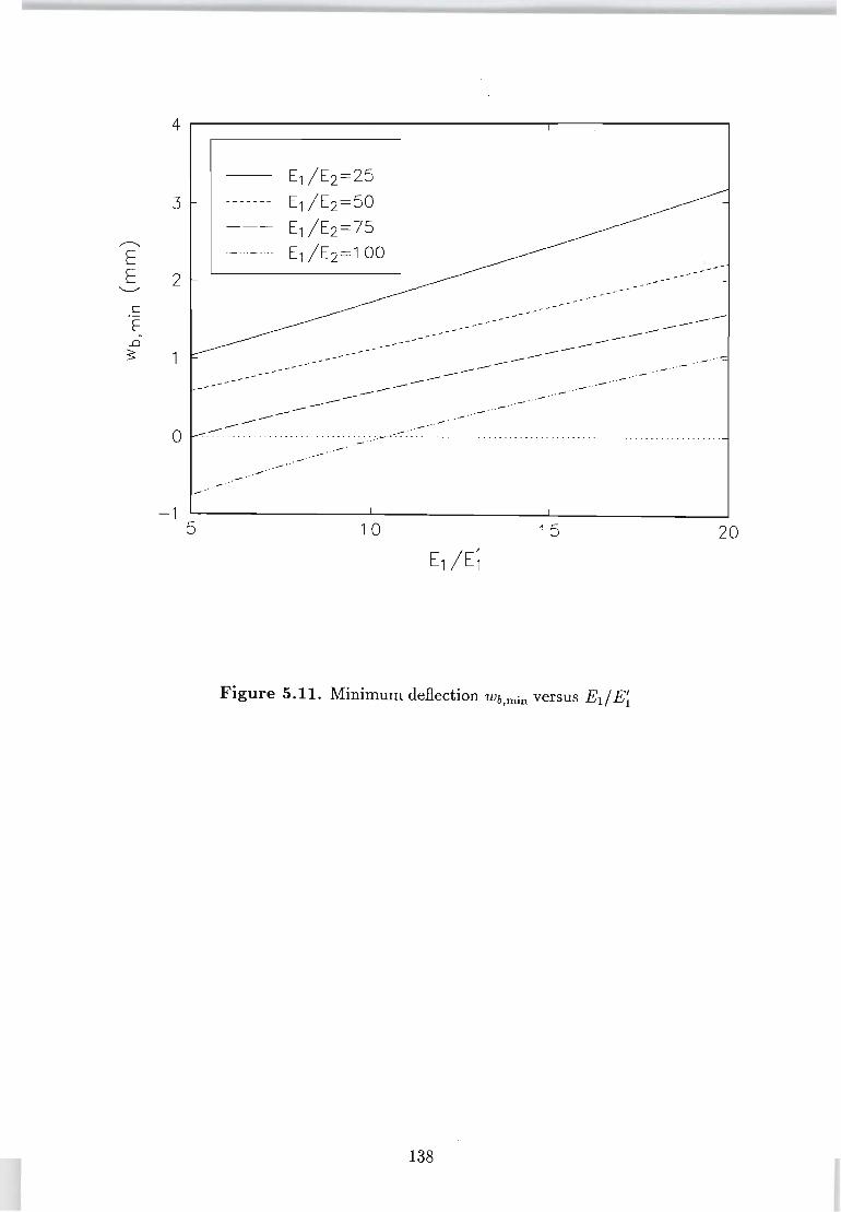
r--...
E E
'--""
c E -.n
3:
4~----------~-------------r--~------~
3
2
o
-1 5
E1/E2=25 ------- E1/E2=50
--- E1/E2=75 ._ ... _ ... - E1 /E2=1 00
-~~
~~~
-----------------
--- ------------------- .. . -
... ---... - .- " ... -
-- .. -" .. ~ .......... . .. . ........... .... ::~ ..•.. -:: -.... _ .... .. ........... _ . ... - .. _ ...... _ ... -.- ...... . ...... . ,.--
--10 15 20
Figure 5.11. Minimum deflection Wb,min versus Ed E~
138
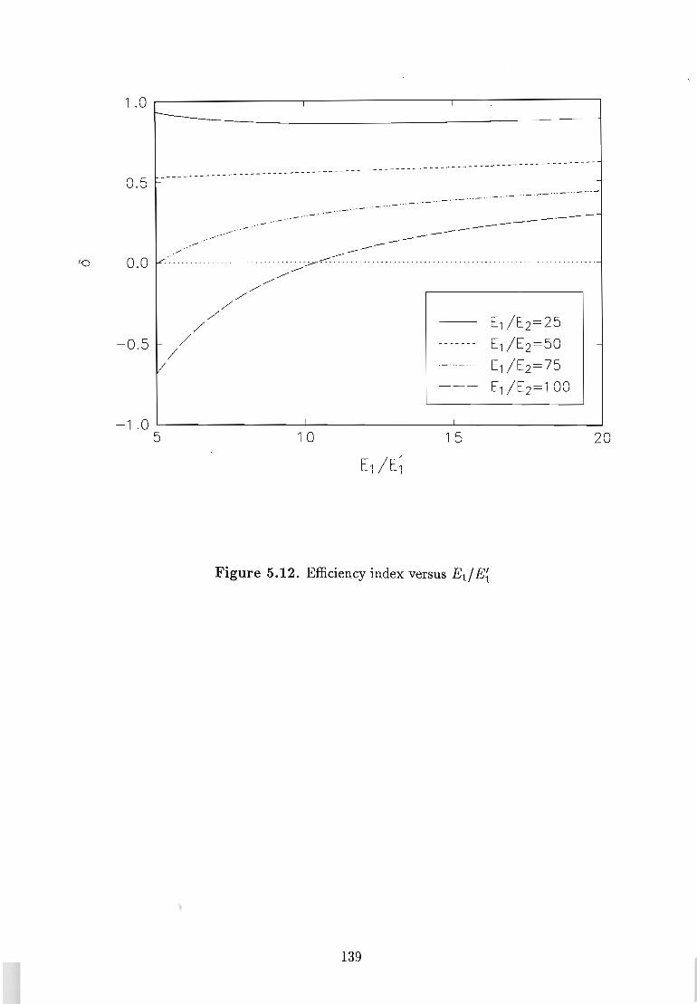
1 .0 .----------,----------,---:--------,
-----------------------------------------------1
- -- ---- --------- --- -- ------------------------- ------ - --- --- -- ---- --
0.5
----------------- --_ .. .-
.. / ----0 .0 ~: .................. ..... ... .. :..:..:_ . ..;.--~ ........ ... ... ..... ...... ...... ........ ...... ... ....... ..... .
-05 / . / V
/' /
./ /'
/"" /""
./
E1 / E2=25
E1/E2=50
E1/ E2 =75
E1 / E2= 100
-1.0 ~------________ L-______________ ~ ____________ ~
5 1 0 1 5 20
Figure 5.12. Efficiency index versus Ell E~
139
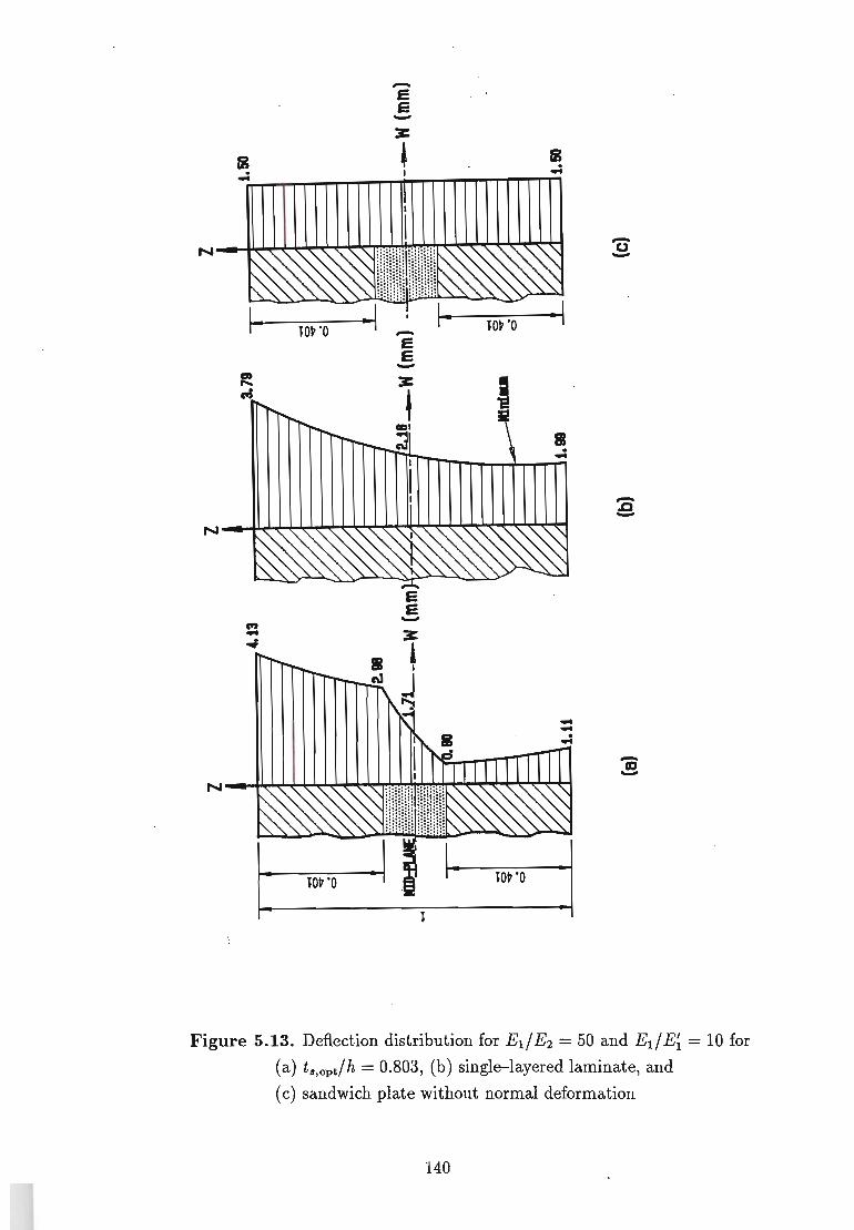
-e e -
. -~~~~~TTTT~III1I1I1IiIi"-
JO~'O -e e -
e e -
JO~'O
II . -
"0 -
'ii -
Figure 5.13. Deflection distribution for Ed E2 = 50 and Ed E~ = 10 for
(a) tlJ,opt/h = 0.803, (b) single-layered laminate, and
( c) sandwich plate without normal deformation
140

-e e -
-nE'O
e e nE'O -
:c -
-e e -
nE'O fl'E'O
Figure 5,14, Deflection distribution for Ed E2 = 90 and Ed E~ = 5 for
(a) t&,opt/h = 0.683, (b) single-layered laminate, and
( c) sandwich plate without normal deformation
141
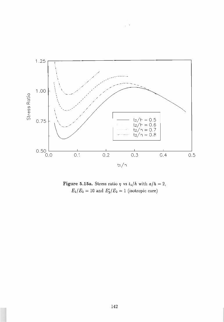
0 +-' 0
0:::: en (f)
Q) I.....
+-' (f)
1 .25
\ , , \ , ,
1 .00 , \ / , , -.. - ...-, , \ \ \ \ /
\ / , , , -. --'
,
0.75 /
,.-, ...--.-
/
/
/ /
/ /
/ /
/ /
/ / /
/
/
/
/
/
, , , , /
/
,.-/
/
, ,
,.-
_ .- ---- . ...-
b/h = 0 .5 b/h = 0 .6 b/h = 0.7 b/h = 0.8
0.50 ~------~--------~--------~--------~------~ 0.0 0.1 0.2 0.3 0.4
b/h
Figure S.lSa. Stress ratio 17 vs tl/h with a/h = 2,
El / E2 = 10 and E~/ E2 = 1 (isotropic core)
142
0.5
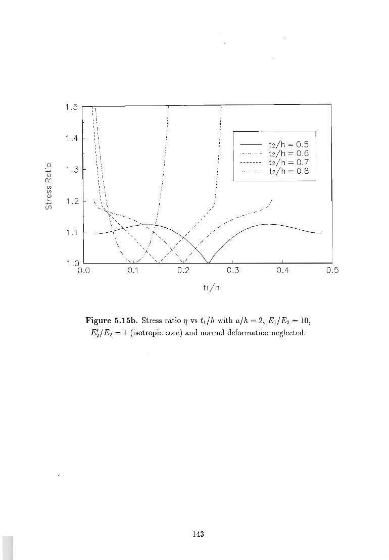
o
1.5~~----------'---------~----------------1 , I
1.4
1 .3
1 .2
1 .1
, : ~ i , : ! \ I:
~ \ , : ~ \
, ~ \ , .
'. .. \ ...... . ~.~- . -
." ''. , \ '
\
, , ,
"- /
0.1
/ /
/
I /
/
I I I I I I I I I I
I /
/ " " /
/
b/h
" .-
b/h = 0.5 b/h = 0 .6 b/h = 0.7 b /h = 0.8
/
Figure 5.15b. Stress ratio TJ vs tdh with alh = 2, Ed Ez = 10, E~I Ez = 1 (isotropic core) and normal deformation neglected.
143

0 +-' 0
0:::: (f) (f)
Q) ~
+-' U)
2.0 .---....... ,-\~--------------------:~ ,
1 .5
1.0
0.5 0.0
\
\
\
\
, , , , , , ,
\
\
, , , , \
\ \
\
\
\ \ \ \ \ , ,
\
\
\
, ", , , , , ---.- .-.- .- ._ .- .- '
0.1
o/h = 2 ._._._.- o/h = 3
o/h = 4 ._ ... _ .... o/h = 5
-.-
0.2 0 .3
I I
/
0.4
I I
I
, , , I
I
Figure 5.16a. Stress ratio TJ vs tl/h with t2/h = 0.5, El / E2 = 100
and E~/ E2 = 10 (transversely isotropic core)
144
0.5
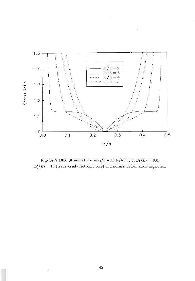
0 +-' 0
n::: (f) (f) Q) I-
+-' (f)
1 .5 ~~---,~-----------------------------r'--:--r-l
1.4
1 .3
1 .2
1 . 1
\
\
\
\
\
\
, \ \ \ , \ \
\
\ \
\
, , \
\
\
\ \ \ ,
. ..... .
0.1
\
.....
\ \
\ \
.-._-- ---------
._ .. __ .. _-
\
0.2
o/ h 2 -
o/ h = 3 o/ h 4 -
o/ h - 5
0.3
/ I
I
I I
I
I I
I
I
I
I I
I I
I I
, I ,
I I I I I I I
, I
I I
I I I
I I I I
I
I
I
I
I
0 .4 0 .5
Figure S.16b. Stress ratio 11 vs tl/h with t2/h = 0.5, El / E2 = 100,
E~/ E2 = 10 (transversely isotropic core) and normal deformation neglected.
145
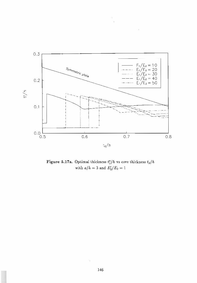
..c '-...... *~ -+-'
0.3 ,.--------------------------,
0 .2
0.1
r ·-.
. - . - . .c.-':. __ -.r--::-:::-::::,~ ... 1'- · 1--.:----..:.:.:..-
E1/E2 = 10 ._._._.- E1/E2 = 20 ------- E1/E2 = 30 --- E1/E2 = 40 .- ... -.. .. E1/E2 = 50
I - 0"""1 0_ - .... ----:.:-::::::..::.-
i "- '- . -- ...... ~ ... -
I I I I 1
I-------------'--~ .. - ... - .:
0 .0 ~--------------~--------------~--------------~ 0.5 0.6 0 .7
h/h
Figure 5.17a. Optimal thickness tUh vs core thickness t2/h with a/h = 3 and E~/ E2 = 1
146
0.8
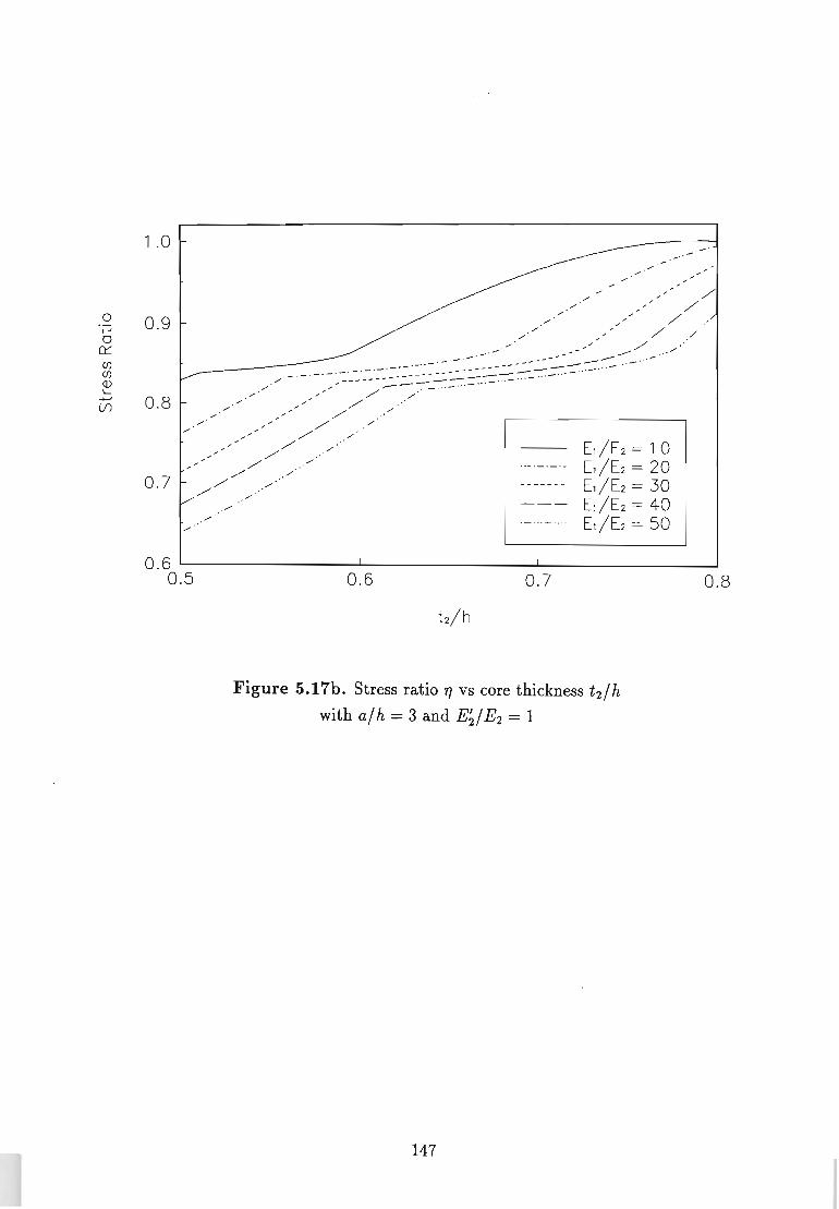
o
1 .0
0.9
0.8
0.7
E1/E2 = 10 E1/E2 = 20 E1/E2 = 30 E1/E2 = 40 E1/E2 = 50
0.6 ~--------------~--------------~--------------~ 0.5 0.6 0.7
h/h
Figure 5.17h. Stress ratio TJ vs core thickness t2/h
with a/h = 3 and E~/E2 = 1
147
0.8
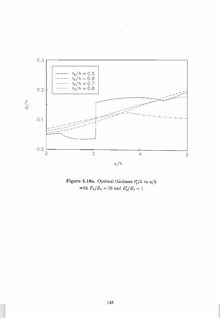
0.3~----------------------------------------,
0.2
0.1
-- '- -
h/h = 0.5 ._._._ .- t2/h = 0 .6 ------- tz/h = 0.7 ._ ... _.... h / h = 0.8
--,- _.- " _ .-"
.. _ ... - ... - .. . - ... _ ... -
0.0 L-______________ ~ ______________ ~I ____________ ~
234
a/ h
Figure 5.18a. Optimal thickness t'Uh vs alh with Ell E2 = 10 and E~I E2 = 1
148
5
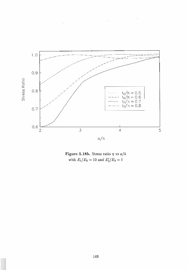
0 +-' 0
n::: (f) (f)
Q) I...
+-' (f)
1 .0 -... -
0.9
0.8 /'
/'
/' /'
/'
0.7 -
.- ... - .. __ ... _ -.. - -
/' /'
/'
/' /'
/ /
/ /
/'
:';':":='-~'=':.:':'~.- - - -- - - - - - - - - - -.---.~-. ~-.- --.; =-.: =- .:. :-.:.:~ -= ~
t2/h = 0.5 .- .- ._-- t2/h = 0_6
tz/h = 0.7 ---- -- --_. tz/h = 0 .8
0.6 ~~------------~--------------~--------------~ 2 3 4
a/h
Figure 5.18b. Stress ratio "7 vs a/h with El / E2 = 10 and E~/ E2 = 1
149
5
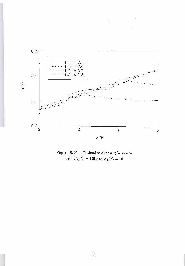
0 .3 ~----------------------------------------------,
h/ h = 0.5 .- .- .- .- h / h = 0.6 ------- h / h = 0 .7
0.2 .- ... - ... - h / h = 0.8
---'--
.. - .. _- "- ... - -. - ... - ... - .. . - " - "' - "' - -- ..
0.0 ~--------------~----__________ -L ______________ ~
2 3 4
a/ h
Figure S.19a. Optimal thickness tUh vs ajh with Ed E2 = 100 and E~j E2 = 10
150
5
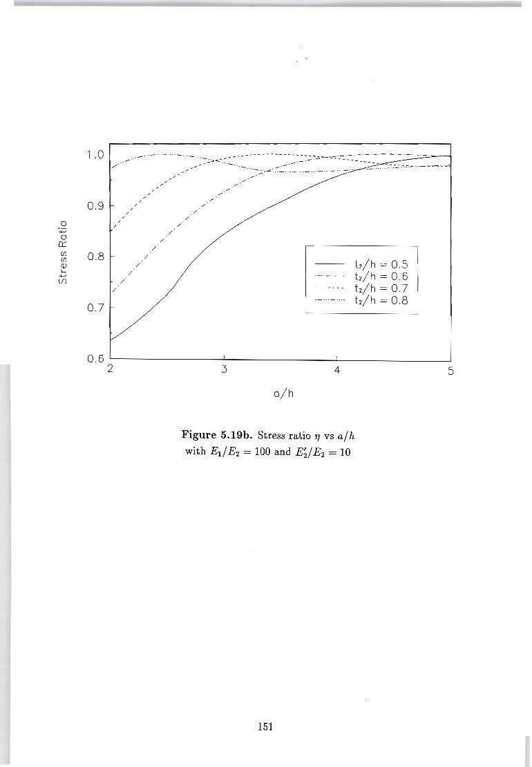
0 ...... 0
0:::: (f) (f)
Q) ~ ......
(f)
1 .0 .-./
, 0 .9 , ,
/ , /
/
0 .8 /
/
/
/
0. 7
.. - _" - "0 _ .
, , , , , , , , ,
/
/
/
/
/
---.;.",, <.~:::-
,.-,.-
,.-,.-
,.-/
/
---- ---- ---- - -:- ~.;:oo-- ~-= - -- ' - ' - ' - ' - ' - -_ .- .
tz/ h = 0.5 ._.- .- .- tz/ h = 0.6 ----- -- tz/ h = 0 .7 ._ ... _.... tz/ h = 0 .8
-----,
0 .6 ~--------------~----------------~--------------~ 2 3 4
a/ h
Figure 5.19b. Stress ratio." vs a/h
with El / E2 = 100 and E~/ E2 = 10
151
5
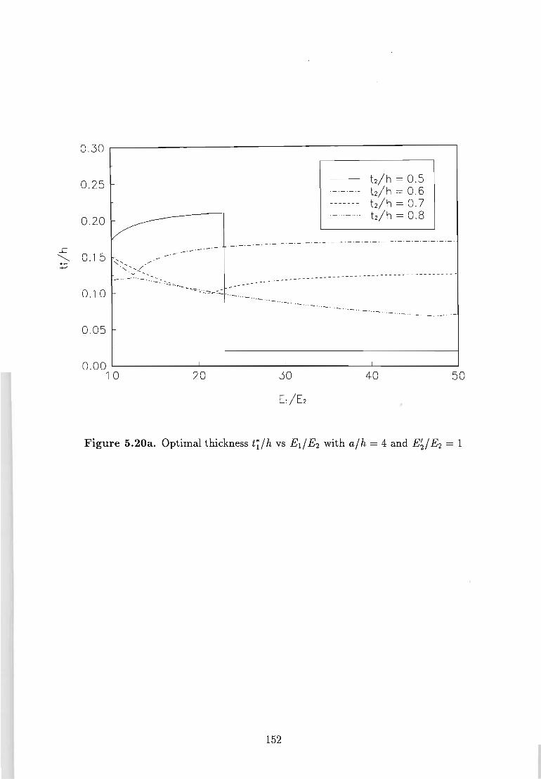
....c:
0 .30 ...---------------------------,
0.25
0.20 v----_ . - '-'-
tz/h = 0 .5 tz/h = 0 .6 tz/h = 0.7 tz/h = 0 .8
-.- . - -_ . - . _ -_ . - . - ._. -._ . _ . _ --. - _.-.- . - . _ .
'---- 0 .15 _.-"
.~
+-' -------------------------------------
0 .1 0 - "' -
- "' - " .. - ... - ... - ... - ... - ... - ... -
0.05
0 .00 L-...-_____ ..I.....-_____ ..I.....-_____ -L--____ -----I
10 20 30 40 50
El/E2
Figure 5.20a. Optimal thickness tUh vs El / E2 with a/h = 4 and E~/ E2 = 1
152
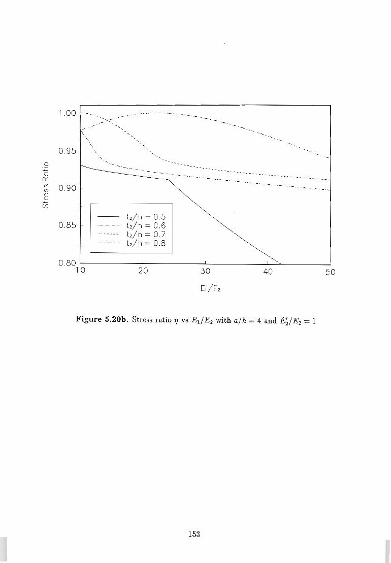
1 .00 --- .. - " .- ... - .. - "' -
"' :-.~ " .- " - "--- -, "-, - , , '-, ,
\ , , , '-\ ,
0.95 , -\ , '-, , -" -
" 0 +-' 0 - - -- -- -- . -
0::: (f) 0.90 (f) Q) L
+-' U)
tz/ h = 0.5 0.85 __ 0 _ 0 _0- t2/ h = 0.6
------- tz/ h = 0.7 . _0 -. _ .... tz/ h = 0.8
0.80 1 0 20 30 40 50
E1 / E2
Figure 5.20b. Stress ratio 7J vs Ed E2 with a/h = 4 and E~/ E2 = 1
153
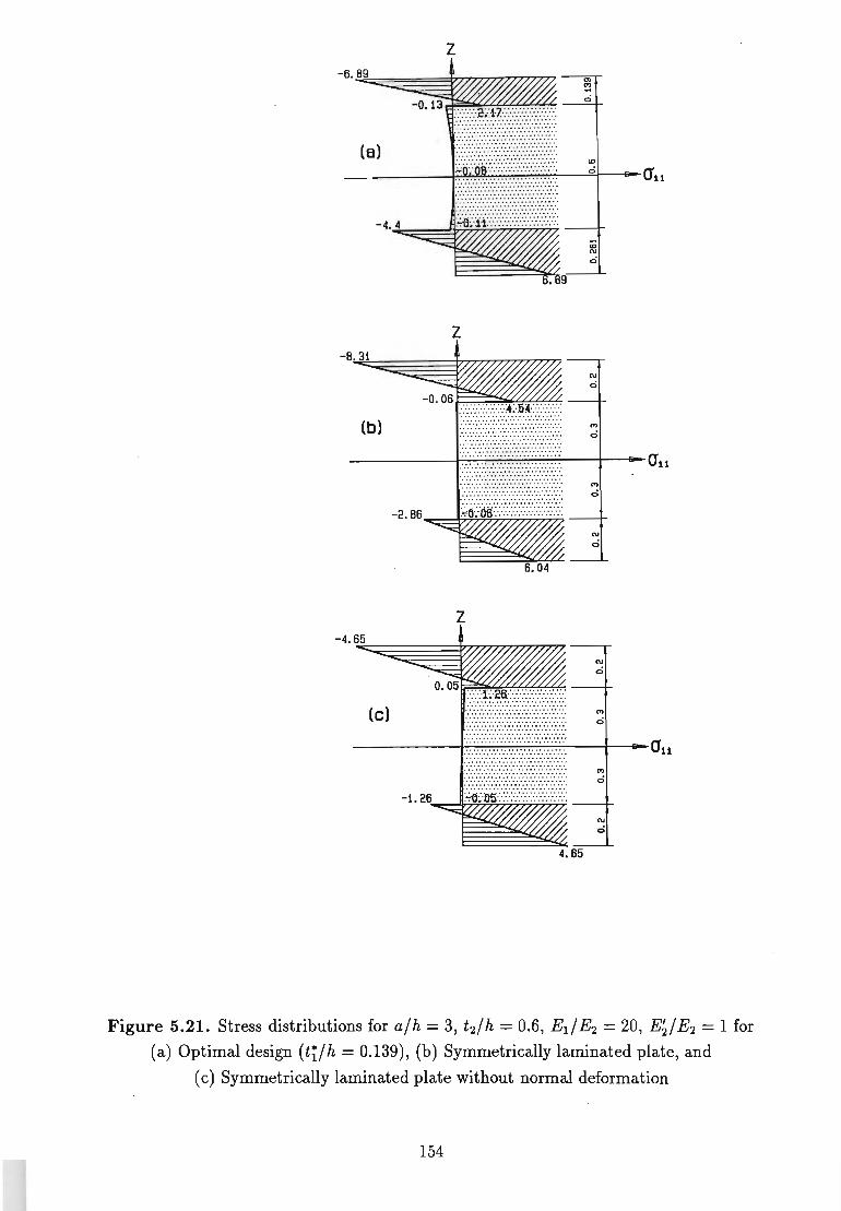
-6.89
(a)
-4.4
-8 31
(b)
Z
z
... .. ............ .... .. ... '::::::::.'.': :.'::::.': ::.'.'.'.' . ............. ....... ...... ... ........ ............ .... :::::::: ::. ':::::.':.'::::.'::.
en ~ 0
'" 0 O'u
-co N
0
N
o
'" o ------F.:.:-::.:..;.:.: . .:.:..::-:.::.:..;.:.: . .:.:..::.:-: . .:.:..::-:.::.:..;.:.: . .:.:..::-:.:~.:.:-:-:-,:.:-:.---11----AU
:::::::::::::::::::::::::::::::::::::::::::::::::::::
(e)
..... .. ... .......... .. .... ............... ...... ..... .... ......... .. ...... .... . ....... ..... .... .. .. ...... ....... ... .. .... .... ......
z
.................... .... .. .................. .... .. .. .... ........ .. ... ..... ... . ......... .... ..... .. .. .... .. .... .. ... .. .... .... ..... ............. .. .. ... ...... ... ........ ...............
....... .. ... .... .......... ........... ..... ..... ... ...
'" o
N
o
N
o
'" c:i
------+.:-.:.: .:~.:.:.~:.:.:~.:.:.:":"::.:.:"7':'.:.:.::':":.:.:.~:.:.:~.:.:.:":"::.:.:-. --+--t-O'u ...... .... ........ ...... .. ...... .......... ..... .. .... ......................... .. ....................... ... ..... ..... .. ..... .. .. ...... ... ... ..... ... ... ......... ............. ... ... ... .... . ........ ... ....... ..... ... '" o
N
o
Figure 5.21. Stress distributions for a/h = 3, t2/h = 0.6, Ed E2 = 20, E~/ E2 = 1 for
(a) Optimal design (t'Uh = 0.139), (b) Symmetrically laminated plate, and
(c) Symmetrically laminated plate without normal deformation
154
5.6 Conclusions
Optimal designs of thick sandwich plates are given using the higher-order theory,
which includes the effects of normal deformation as well as transverse shear de
formation. The higher-order theory can provide accurate solutions for very thick
laminates with layers having significantly different mechanical properties. There
fore this approach makes it possible to optimize sandwich plates with thickness
ratio a/h ~ 5.
The higher-order theory is implemented using symbolic computation in preference
to an analytical or numerical method, since deriving the necessary analytical ex
pressions would be extremely cumbersome while a numerical method would to some
extent nullify the accuracy afforded by the higher-order theory. In order to operate
at the highest possible computational efficiency, special purpose symbolic computa
tion routines are developed and incorporated into an optimization algorithm. These
routines bypass some of the symbolic processing which makes the routines developed
in Section 4.5 relatively more flexible, and as such can achieve a higher degree of
efficiency. It is found that the use of a general purpose symbolic computation system
for the present optimization studies is infeasible as it leads to excessive computer
time.
When normal deformation is considered, the through-the-thickness distribution of
the normal stresses ceases to be symmetrical in the case of unsymmetrical loading,
i.e. loading loading on one surface of the plate only, and conventional symmetrical
designs are non-optimal. Moreover, normal deformation results in the bottom sur
face having a minimum deflection at a certain thickness ratio of surface and core
layers and the minimum deflection design is based on this observation. Another
interesting observation is the existence of negative deflection of the bottom surface
at certain stiffness ratios. This phenomenon arises as a result of Poisson's effect on
the normal deformation.
Three design problems are formulated and solved, namely optimal designs for mini
mum weight, minimum deflection and min-max normal stress. The minimum weight
problem involves the determination of the fibre content of transversely isotropic sur
face layers made of a randomly oriented fibre composite material. The other design
variable is taken as the core layer thickness. Minimum weight designs subject to
a deflection constraint are obtained and the effects of problem parameters on the
design variables and weight are studied. It is observed that fibre content decreases
as the sandwich thickness increases for a given deflection.
155
In the minimum deflection problem, the thicknesses of the surface layers are chosen
as the design variables. The effect of the relative stiffness Ell E2 of the surface and
core layers is investigated and it is observed that surface layer thickness is smaller
if the core stiffness E2 is low due to more of the deflection being absorbed by a
softer core region. However, surface layer thickness does not show a definite trend
as the through-the-thickness stiffness E~ of surface layers decreases. This thickness
decreases for low Ed E2 ratios and increases for high Ed E2 ratios as E~ decreases.
The optimal design for minimum stress involves the computation of the relative
thicknesses of the layers such that the maximum normal stress will be minimized.
The resulting design leads to vastly improved sandwich plates which have normal
stresses up to 40% less than those of a symmetrical sandwich. However, the efficiency
drops for a transversely isotropic core as compared to an isotropic core. It is observed
that the thicknesses of the top and bottom layers of an optimal plate depend on
the relative thickness of the core layer, the thickness ratio of the plate and on the
relative stiffness of the core layer as compared to the surface layers. It emerges
that although the top layer on which the load acts is in general thinner than the
bottom layer for a minimum stress design, this is not always the case and the bottom
layer can also be thinner depending on the geometric and material parameters. In
particular this is the case if the core layer is thick compared to the surface layers. It is demonstrated that normal deformation has a substantial effect on the design and
the effect of normal deformation becomes more pronounced when the plate becomes
thicker.
Deflection and stress profiles through the thickness are studied with a view towards
assessing the effect of the configuration on the bottom surface deflection and maxi
mum normal stress and the effect of neglecting normal deformation. It is observed
that if the theory used in the design analysis does not include normal deforma
tion, the design of thick structures becomes meaningless as it leads to non-optimal sandwich plates.
156
Chapter 6
Conclusions
6.1 Overview
In the present study the design optimization of a suite of laminated composite
structures is performed. In the first instance thin laminated composite structures
are optimized, in particular balanced and unbalanced laminated composite pressure
vessels with specially orthotropic layers whose elastic properties depend on the angle
of the reinforcing fibres.
Special purpose symbolic computation routines are developed in a conventional pro
gramming language in order to improve the efficiency of the optimization algorithm.
These routines combine the relationship between the loading parameters and the
stress into one transformation matrix and thereby reduce the number of calcula
tions required in each iteration of the optimization algorithm. It is found that the
development of such routines, which are dedicated to a specific class of functions, is
a feasible objective.
A new higher-order theory which includes the effects of both transverse shear and
normal deformation is developed for the analysis and design optimization of thick
laminated composite structures with transversely isotropic layers. The form of the
kinematic hypotheses of the theory are derived using an iterative technique where
the classical Kirchhoff-Love hypotheses are assumed in the first iteration and new
variables which have a clear physical meaning are introduced. The governing differ
ential equations contain stiffness constants which are integrals through the thickness
of the laminate. The unknown functions in the governing equations are defined on
an arbitrary reference surface and the order of the system of governing equations is
157
independent of the number oflayers. The stress/strain state of a laminated structure
is determined using the kinematic hypotheses which inClude the solution of the gov
erning equations (for the reference surface) and through-the-thickness distribution
functions defined by the theory.
The distribution functions and integrated stiffnesses of the theory are multiple piece
wise integrals through the thickness of the laminate. In the general case, these inte
grals are not able to be derived in a form suitable for exact numerical calculations
and the evaluation of these integrals using a numerical method detracts from the
accuracy afforded by the higher-order theory. These difficulties are overcome by
employing symbolic computation to derive the distribution functions, calculate the
integrated stiffness constants exactly, and derive the stress and strain distributions
through the thickness in power series form, for a given laminate.
In addition to using a general purpose symbolic computation system, special purpose
symbolic computation routines are developed for the implementation of the theory.
These routines are found to be at least two orders of magnitude more efficient in
the performance of the required computations than the general purpose system.
Therefore in optimization studies, where computational efficiency is of paramount
importance, the development of special purpose symbolic computation software is
preferable to using a general purpose symbolic computation system. Moreover,
special purpose symbolic computation routines are easily incorporated into an op
timization algorithm whereas this is not possible using a closed general purpose
system.
The numerical results obtained indicate that the new higher-order theory is accu
rate for thick structures whereas, in general, the shear deformable theory and the
classical theory are inaccurate. Therefore in the analysis of thick structures, not
only transverse shear but also normal deformation should be taken into account.
Sandwich plates of thickness ratio a/ h ::; 5 are optimized for minimum weight,
minimum deflection and minimum stress on the basis of the higher-order theory.
Such designs are not possible using a theory which neglects normal deformation.
6.2 Symbolic Computation
Special purpose symbolic computation software is developed in the C language for
the transformation of coordinate axes, failure analysis and the calculation of design
158
sensitivities for fibre reinforced composite structures. The symbolic computation
routines perform tedious matrix algebra where the entrIes of the matrices are series
of double trigonometric functions and simplify the results using trigonometric iden
tities. The symbolic computations are integrated into an optimization algorithm
resulting in a combined symbolic and numerical approach to determine the optimal
design.
Special purpose symbolic computation routines are also developed for the implemen
tation of the higher-order theory. Symbols may be defined as laminae parameters,
symbolic expressions or piecewise integrals of symbolic expressions. Symbols and
symbolic expressions are recursively expanded into power series which may be inte
grated and evaluated.
6.3 Optimization of Thin Pressure Vessels
Two design problems for thin laminated composite pressure vessels are solved. In
the first problem, a cylindrical pressure vessel is optimized taking the fibre angle
as the design variable to maximize the burst pressure and the effects of the axial
force and torque on the optimal designs are investigated. In the second problem,
a cylindrical vessel filled with liquid and subject to an internal pressure is studied.
The weight of the shell is minimized taking the fibre angle and the wall thickness as
the design variables. Both constant and variable thickness shells are investigated. It
is shown that the results for the second problem approach those of the first problem
as the internal pressure increases.
Numerical results are given for unbalanced (single- and six-layered) and balanced
laminates noting that in the balanced case the number of layers does not affect
the results. It is observed that fibre angles align themselves with the longitudinal
axis as the axial force increases . . Variable thickness shells are found to be about
20% more efficient than the constant thickness shells for low values of the internal
pressure with the difference decreasing as this pressure increases. For single-layered
pressure vessels, the optimal fibre angle is found to be either 00 or 900 with the
switch-over point depending on the magnitude of the axial force, torque and the
internal pressure.
159
6.4 Higher-Order Theory
The numerical results obtained for thick homogeneous and heterogeneous plates are
compared to those given in the literature to validate the higher-order theory. It
is found that for an isotropic plate with thickness ratio a/h = 2, the higher-order
theory predicts the deflection distribution to within 2% and the normal stresses
to within 5% of the exact three-dimensional elasticity solution whereas the shear
deformable model which neglects the effect of normal deformation and the classical
theory are grossly inaccurate.
As the transverse rigidity of plates decreases, the effect of normal deformation be
comes more pronounced and the inaccuracy of the shear-deformable model increases.
However, it is observed that as the ratio a/ h increases, the effect of normal deforma
tion is reduced and, in general, the shear-deformable theory is accurate for plates
with a/h ~ 10.
Numerical results for a sandwich plate where the higher-order theory is used to
model the core layer and the classical theory is used to model the surface layers
are compared to those given in the literature where the core layer is modelled as a
three-dimensional elastic body. It is found that the discrepancies are at most 0.8%
for a/ h = 3, ... ,10 and a core layer up to two orders of magnitude weaker than the
surface layers.
6.5 Optimization of Thick Sandwich Plates
Three design problems are formulated and solved, namely, optimal designs for mini
mum weight, minimum deflection and minimum normal stress. The minimum weight
problem involves the determination of the optimal thickness of the core layer and
the optimal fibre content of the surface layers. It is observed that fibre content
decreases as the sandwich thickness increases for a given deflection constraint.
In the minimum deflection problem, the thicknesses of the surface layers are cho
sen as the design variables. The design optimization is based on the observation
that the deflection of the bottom surface decreases as the core layer becomes thin
ner but increases again once the thickness of the core layer relative to the surface
layers drops below a critical level. Moreover, the bottom surface may undergo neg
ative deflection for certain combinations of material properties. These phenomena
160
are peculiar to thick structures and can only be analysed using three-dimensional
elasticity solutions or a higher-order theory which includes normal deformation.
The optimal design for minimum stress involves the computation of the relative
thicknesses of the layers such that the maximum normal stress will be minimized. It
is demonstrated that normal deformation has a substantial effect on the design and
this effect becomes more pronounced as the thickness of the plate increases. When
normal deformation is taken into account, the maximum normal stresses in the top
and bottom layers are not equal in the case of a symmetrical sandwich. The design
optimization produces a configuration where these maximum stresses are equal and
leads to vastly improved sandwich plates which have normal stresses up to 40% less
than those of a symmetrical sandwich. It is found that if the theory used in the
design analysis does not include normal deformation, the design of thick structures
becomes meaningless as it leads to non-optimal sandwich plates.
161
6.6 Recommendations for Future Work
Higher-order theory for orthotropic materials
The present higher-order theory could be extended to orthotropic materials. This
would enable the optimization of composite structures reinforced with continuous
fibres where the fibre orientation is a design variable. The boundary conditions
could be extended to cylindrical shells for the optimization of pressure vessels.
Object-oriented symbolic computation
The development of special purpose symbolic computation routines lends itself to
wards an object-oriented approach and such routines could be developed using the
C++ language for various applications.
Design optimization of thick structures
A three-dimensional failure criterion could be used as a design constraint for the
optimization studies of thick structures based on the higher-order theory.
The optimization studies could be extended to structures under other loading condi
tions such as uniformly distributed and localized loads and under various boundary
conditions.
162
Bibliography
[1] Pipkin, A. C., & Rivlin, R. S., Minimum~weight design for pressure vessels
reinforced with inextensible fibres. J. Applied Mechanics, 30 (1963) 103-108.
[2] Chao, C. C., Sun, C. T., & Koh, S. L., Strength optimization for cylindrical
shells of laminated composites, J. Composite Materials, 9 (1975) 55-66.
[3] Urazgil'dyaev, K. U., Design of a equal-strength cylindrical shells of composite
material. Prikladnaya Mekhanika, 13 (7) (1977) 121-124.
[4] Tauchert, T. R., Optimum design of a reinforced cylindrical pressure vessel. J.
Composite Materials, 15 (1981) 390-402.
[5] Fukunaga, H., & Uemura, M., Optimum design of helically wound composite
pressure vessels. J. Composite Structures, 1 (1983) 31-49.
[6] Eckold, G. C., A design method for filament wound GRP vessels and pipework.
Composites, 16 (1) (1985) 41-47.
[7] Fukunaga, H., & Chou, T. W., Simplified design techniques for laminated cylin
drical pressure vessels under stiffness and strength constraints. J. Composite
Materials, 22 (1988) 1157-1169.
[8] Karandikar, H., Srinivasan, R., Mistree, F., & Fuchs, W. J., Compromise: An
effective approach for the des,ign of pressure vessels using composite materials.
Computers & Structures, 33 (6) (1989) 1465-1477.
[9] Adali, S., & Yakar, B., Optimal design of laminated pressure vessels under
internal pressure and temperature loading. In Pressure Vessels and Components
1991, Proc. of the 1991 Pressure Vessels and Piping Conference, PVP-Vol. 217,
ASME, New York (1991) 57-63.
[10] Adali, S., Fuzzy optimization of laminated cylindrical pressure vessels. In Com
posite Structures 6, Proc. of the 6th International Conference on Composite
Structures, Elsevier Applied Science, London (1991) 249-259.
163
[11] Datoo, M. H., Mechanics of Fibrous Composites. Elsevier Applied Science, Lon
don, 1991.
[12] Tsai, S. W., & Hahn, W. T., Introduction to Composite Materials. Technomic
Publishing Company, Westport, Connecticut, 1980.
[13] Fliigge, W., Stresses in Shells. 2nd Edition, Springer-Verlag, New York, 1973.
[14] Kraus, H., Thin Elastic Shells. John Wiley & Sons, New York, 1967.
[15] Beltzer, A.1. , Engineering analysis via symbolic computation - a breakthrough.
Appl. Mech. Rev., 43 (6) (1990) 119-127.
[16] Crespo da Silva, M. R. M., & Hodges, D. H., The role of computerized symbolic
manipulation in rotorcraft dynamic analysis. Compo Math. Appl., 12A (1986)
161-172.
[17] Elishakoff, I., & Halkamp, J., Computerized symbolic solution for a monconser
vative system in which instability occurs by flutter in one range of the parameter
and by divergence in the other. Computer Meth. Appl. Mech. Eng., 62 (1987)
27-46.
[18] Elishakoff, I., & Couch, B., Application of computerized symbolic algebra for
instability of nonconservative systems. J. Symbolic Comp., 4 (1987) 391-396.
[19] Elishakoff, I., & Tang, J., Buckling of polar orthotropic circular plates on elastic
foundation by computerized symbolic algebra. Computer Meth. Appl. Mech.
Eng., 68 (1988) 229-247.
[20] Elishakoff, I., & Pletner, B., Computerized symbolic algebraic evaluation of
buckling loads by Snitko's method. Computer Meth. Appl. Mech. Eng., 88
(1991) 299-309.
[21] Graaf, E., & Springer, G. S., Stress analysis of thick curved composite lami
nates. Computers and Structures, 38 (1) (1991) 41-55.
[22] Nomura, S., & Wang, B. P., Free vibration of composite plates using symbolic
algebra. Advanced Composite Materials, 1 (1991) 87-92.
[23] Wolfram, S., Mathematica: A System for Doing Mathematics by Computer.
Addison-Wesley (1988).
[24] Summers, E. B., Adali S., & Verijenko, V. E., Special purpose symbolic com
putation software with application to the optimization of composite laminates.
Advances in Engineering Software, 18 (1993) 199-209. .
164
[25] Dudchenko, A. A., Lur'e, S. A., & Obraztcov, 1. F., Anisotropic multilayer
plates and shells. Summary of science and engineering. M echanica Deformirue
mogo Tela, 15 (1983) 3-68 (in Russian).
[26] Librescu, L., & Reddy, J. N., A few remarks concerning several refined theories
of anisotropic composite laminated plates. Inti. J. Engrg. Sci., 27 (5) (1988)
515-527.
[27] Reddy, J. N., A review of refined theories of laminated composite plates. Shock
Vib. Dig., 22 (7) (1990) 3-17.
[28] Noor, A. K., & Burton, W. S., Assessment of computational models for multi
layered composite shells. Appl. Mech. Rev., 43 (4) (1990) 67-97.
[29] Bolotin, V. V., & Novichkov, U. N., Mechanics of Multilayered Structures.
Mashinostroenie, Moscow, 1980 (in Russian).
[30] Grigorenko, J . M., & Vasilenko, A. T., Methods for Shell Analysis. Volume 4· Theory for Shells with Variable Stiffnesses. Naukova Dumka, Kiev, 1981 (in
Russian).
[31] Piskunov, V. G., & Verijenko, V. E., Linear and Non-linear Problems in the
Analysis of Laminated Structures. Budivelnik, Kiev, 1986 (in Russian).
[32] Reissner, E., On bending of elastic plates. Quart. Appl. Mech., 5 (1) (1947)
55-68.
[33] Mindlin, R.D., Influence of rotatory inertia and shear on flexural motions of
isotropic elastic plates. J. Appl. Mech., Trans. ASME., 18 (1951) 31-38.
[34] Gol'denveizer, A. L., Derivation of an approximate theory of bending of plates
by the method of assymptotic integration of the equations of the theory of
elasticity. PMM, 26 (4) (1963) 1000-1025.
[35] Reddy, J. N., A general nonlinear third-()rder theory of plates with moderate
thickness. J. Non-Linear Mechanics, 25 (6) (1990) 677-686.
[36] Ambartsumyan, S. A., Some Basic Equations for a Theory of Thin Laminated
Shells. Dokl. Akad. Nauk ASSR, 8 (5) (1948) 203-210 (in Russian).
[37] Ambartsumyan, S. A., General Theory of Anisotropic Shells. Nauka, Moscow.
446p (1974) (in Russian).
165
[38] Vasilenko, A. T., & Savchenko, P. 1., Axisymmetric deformation of layered
anisotropic shells of revolution with allowance for transverse shear strains and
contraction. Prikladnaya Mekhanika, 24 (5) (1988) 499- 504.
[39] Grigorenko, J. M., Vasilenko, A. T., & Golub, G. P., Computing the stressed
state of orthotropic elements of shell designs with allowance for transverse shear
and reduction. Mechanics of Composite Materials, 22 (3) (1986) 338-343.
[40] Stein, M., Nonlinear theory for plates and shells including the effects of trans
verse shearing. AIAA J., 24 (9) (1986) 1537-1544.
[41] Reddy, J. N., On refined theories of composite laminates. Meccanica, 25 (4)
(1990) 230-238.
[42] Piskunov, V. G., Variant of the nonclassical theory of multilayered shallow
shells and plates. Soviet Appl. Mech. , 15 (11) (1979) 1073-1078.
[43] Rasskazov, A. 0., Theory of multilaminate orthotropic sloping shells. Soviet
Appl. Mech., 12 (11) (1976) 50- 56.
[44] Piskunov, V. G., Verijenko, V. E., Adali, S., & Summers, E. B., A higher-order
theory for the analysis of laminated plates and shells with shear and normal
deformation. Inti. J. Engrg. Sci., 31 (6) (1993) 967-988.
[45] Verijenko, V. E., Nonclassical theory of elasto-:plastic strain of laminated trans
versely isotropic tapered shells. Strength of Materials, 19 (4) (1987) 547-553.
[46] Verijenko, V. E., & Piskunov, V. G., Geometrically nonlinear theory of shallow
multilayered orthotropic shells. Strength of Materials, 21 (1) (1989) 8-16.
[47] Verijenko, V. E., Adali, S. , & Summers, E. B., Nonlinear analysis of laminated
composite plates and shells including the effects of shear and normal deforma
tion. Composite Structures, 25 (1993) 173-185.
[48] Blocki, J., A higher order linear theory for isotropic plates. 1. Theorectical
considerations. Inti. J. Solids (3 Struct. , 29 (1992) 825-836.
[49] Librescu, L., & Schmidt, R. , Substantiation of a shear deformable theory of
anisotropic composite laminated shells accounting for the interlaminae conti
nuity conditions. Inti. J. Engr. Sci., 29 (1991) 669-683.
[50] Tessler, A., & Saether, E., A computationally viable higher order theory for
laminated composite plates. Inti. J. Num. Meth. Engr., 31 (1991) 1069-1086.
166
[51] Novozhilov, V. V. , Theory of Thin Shells. Gossouziz<iatsudprom, Leningrad,
1962 (in Russian).
[52] Vlasov, B. F., About one case of bending a rectangular thick plate. Vest.
Moscow University. 2 (1957) 22-34 (in Russian).
[53] Brukker, L. E., Some variants of the equations for three-layered plates. Analysis
of Aerospace Structures. 3 (1965) 74- 99 (in Russian).
[54] Bhimaraddi, A., Static and transient response of rectangular plates. Thin
Walled Struct., 5 (1987) 125-143.
[55] Lo, K. H., Christensen, R. M., & Wu, E. M., A higher order theory of plate
deformation. Part 2. Laminated plates. J. Appl. Mech., Trans. ASME., 44 (4)
(1977) 669-676.
[56] Piskunov, V. G., Verijenko, V. E., & Prisyazhnyuk, V. K., Calculation of In
homogeneous Shells and Plates 1l;sing Finite Element Methods. Veisha Shkola,
Kiev, 1987 (in Russian).
[57] Verijenko, V. E., & Prisyazhnyuk, y. K., Linear and nonlinear models of contact
interaction of laminated constructions with elastic basement. Proceedings of
International Congress IKM-X, Weimar, Germany, 6 (1984) 175-182.
[58] Verijenko, V. E., Adali, S., & Summers, E. B., -Discrete-continuous scheme
of FEM for analysing laminated composite shells and plates. Proceedings of
FEMSA92, Cape Town, South Africa (1992) 589-600.
[59] Voyiadjis, G. Z., & Baluch M. H., Refined theory for thick composite plates.
ASME J. Engr. Mech., 114 (4) (1988) 671-687.
[60] Verijenko, V. E., Adali, S., & Summers, E. B., Applications of refined the
ory in the nonlinear analysis of composite laminated structures. Computational
Mechanics, 14 (1994) 52-67.
[61] Summers, E. B., & Verijenko, V. E., Symbolic computation in numerical anal
ysis of composite plates and shells. Proc. 18th SANUM Symposium, Durban, South Africa (1992).
[62] Verijenko, V. E., Adali, S., & Summers, E. B., Investigation of the conver
gency of numerical methods applied to nonlinear problems in the mechanics of
composites. Proc. 18th SANUM Symposium, Durban, South Africa (1992).
167
[63] Adali, S., Summers, E. B., & Verijenko, V. E., Optimization of laminated
cylindrical pressure vessels under strength criterion. Composite Structures, 25
(1993) 305-312.
[64] Verijenko, V. E., Summers, E. B., & Adali, S., Symbolic computation for the
optimization of composite structures using higher order theory. International
Congress on Computer Systems and Applied Mathematics, St Petersburg, Rus
sia, July 1993 (Abstract).
[65] Summers, E. B., Verijenko, V. E., & Adali, S., The development of sym
bolic computation routines using the C programming language. International
Congress on Computer Systems and Applied Mathematics, St Petersburg, Rus
sia, July 1993 (Abstract).
[66] Verijenko, V. E., Adali, S., Stewart, R. W., & Summers, E. B., Application of
the method of initial functions to the analysis of anisotropic plates. 19th South
African Symposium on Numerical Methods, San Lameer, South Africa, July
1993 ( Abstract).
[67] Pandya, B. N., & Kant, T., Higher-order shear deformable theories for flexure
of sandwich plates - Finite element evaluations. Int. J. Solids Structures, 24
(12) (1988) 1267-1286.
[68] Gordaninejad, F., & Bert, C. W., A new theory for bending of thick sandwich
beams. Int J. Mech. Sciences, 11/12 (1989) 925-934.
[69] Bert, C. W., & Cho, K. N., Uniaxial compressive and shear buckling in or
thotropic sandwich plates by an improved theory. Mechanics of Structures and
Machines, 17 (3) (1989) 283-302.
[70] Huang, S. N., & Alspaugh, D. W., Minimum weight sandwich beam design.
AIAA Journal, 12 (12) (1974) 1617-1618.
[71] Vinson, J. R., Optimum design of composite honeycomb sandwich panels sub
jected to uniaxial compression. AIAA Journal, 24 (10) (1986) 1690-1696.
[72] Ding, Y. Optimum design of honeycomb sandwich constructions with buckling
constraints. Computers and Structures, 33 (6) (1989) 1355-1364.
[73] Martin, P. M. J. W., Optimum design of anisotropic sandwich panels with thin . faces. Engineering Optimization. 11 (1987) 3-12.
[74] Makris, S. E., MacGregor Smith, J., & Dym, C. L., Multiobjectiveoptimization
of acoustic sandwich panels. Engineering Optimization, 13 (1988) 147-172.
168
[75] Min, K. T., & de Charentenay, F. X., Optimum weight design of sandwich
cylinders with orthotropic facings and core under combined loads. Computers
and Structures, 24 (2) (1986) 313-322.
[76] Evans, K. E., The design of doubly curved sandwich panels with honeycomb
cores. Composite Structures, 17 (1991) 95-111.
[77] Adali, S., Richter, A., & Verijenko, V. E., Non-probabilistic modelling and
design of sandwich plates subject to uncertain loads and initial imperfections.
Submitted to Int. J. Engineering Science.
[78] Adali, S., Design of shear-deformable antisymmetric angle-ply laminates to
maximize the fundamental frequency and frequency separation. Composite
Structures, 2 (1984) 349-369.
[79] Kam, T. Y., & Chang, R. R., Design of laminated composite plates for max
imum buckling load and vibration frequency. Computer Methods in Applied
Mechanics and Engineering, 106 (1993) 65-81.
[80] Kam, T. Y., & Chang, R. R., Buckling of shear deformable laminated composite
plates. Composite Structures, 22 (1992) 223-234.
[81] Kam, T. Y., & Chang, R. R., Optimum layup of thick laminated composite
plates for maximum stiffness. Engineering Optimization, 19 (1992) 237-249.
[82] Berlin, A. A., Volfson, S. A., Enikolopian, N. S., & Negmatov, S. S., Principles
of Polymer Composites. Springer-Verlag, Heidelberg, 1986.
[83] Chamis, C. C., Simplified composite micromechanics equations for mechanical,
thermal and moisture-related properties. In Engineers' Guide to Composite
Materials, edited by J. W. Weeton, D. M. Peters & K. 1. Thomas. American
Society for Metals, Metals Park, Ohio, 1987, pp. 3/8-3/24.
[84] Plantema, F. J., Sandwich Construction. John Wiley & Sons, New York, 1966.
[85] Adali, S., Summers, E. B., & Verijenko, V. E., Minimum weight and deflection
design of thick sandwich laminates via symbolic computation. To appear in Composite Structures.
[86] Verijenko, V. E., Adali, S., Summers, E. B., & Reiss, T., Optimal design of
laminated shells with shear and normal deformation using symbolic computa
tion. Proceedings of 5th AIAA/USAF/NASA/ISSMO Symposium on Multidis
ciplinary Analysis and Optimization, Panama City Beach, Florida, September 1994.
169
[87] Verijenko, V. E., Summers, E. B., & Adali, S., Minimum stress design of trans
versely isotropic sandwich plates based on higher-order theory. Submitted to
Composites Engineering.
[88] Adali, S., Richter, A., Summers, E. B., & Verijenko, V. E., Optimal design
of hybrid laminates with discrete ply-angles for minimum buckling load. (In
preparation. )
170
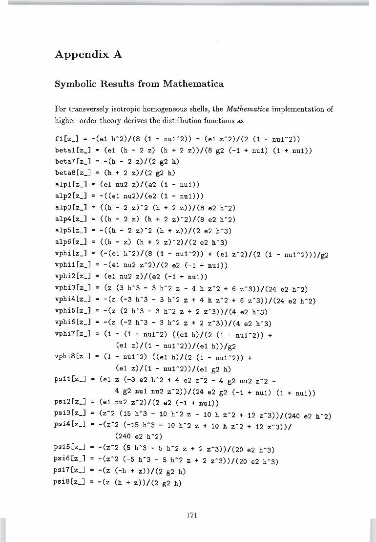
Appendix A
Symbolic Results from Mathematica
For transversely isotropic homogeneous shells, the Mathematica implementation of
higher-order theory derives the distribution functions as
fl[z_] = -(el h~2)/(8 (1 - nul~2)) + (el z~2)/(2 (1 - nul~2))
betal[z_] = (el (h - 2 z) (h + 2 z))/(8 g2 (-1 + nul) (1 + nul)) beta7[z_] = -(h - 2 z)/(2 g2 h)
beta8[z_] = (h + 2 z)/(2 g2 h)
alpl[z_] = (el nu2 z)/(e2 (1 - nul))
alp2[z_] = -«el nu2)/(e2 (1 - nul)))
alp3[z_] = «h - 2 z)~2 (h + 2 z))/(8 e2 h~2)
alp4[z_] = «h - 2 z) (h + 2 z)~2)/(8 e2 h~2)
alp5[z_] = -«h - 2 z)~2 (h + z))/(2 e2 h~3)
alp6[z_] = «h - z) (h + 2 z)~2)/(2 e2 h~3)
vphi[z_] = (-(el h~2)/(8 (1 - nul~2)) + (el z~2)/(2 (1 - nul~2)))/g2
vphil[z_] = -(el nu2 z~2)/(2 e2 (-1 + nul))
vphi2[z_] = (el nu2 z)/(e2 (-1 + nul))
vphi3[z_] = (z (3 h~3 - 3 h~2 z - 4 h z~2 + 6 z~3))/(24 e2 h~2)
vphi4[z_] = -(z (-3 h~3 - 3 h~2 z + 4 h z~2 + 6 z~3))/(24 e2 h~2) vphi5[z_] = -(z (2 h~3 - 3 h~2 z + 2 z~3))/(4 e2 h~3)
vphi6[z_] = -(z (-2 h~3 - 3 h~2 z + 2 z~3))/(4 e2 h~3)
vphi7[z_] = (1 - (1 - nul~2) «el h)/(2 (1 - nul~2)) +
(el z)/(l - nul~2))/(el h))/g2 vphi8[z_] = (1 - nul~2) «~1 h)/(2 (1 - nul~2)) +
(el z)/(l - nul~2))/(el g2 h) psil[z_] = (el z (-3 e2 h~2 + 4 e2 z~2 - 4 g2 nu2 z~2 -
4 g2 nul nu2 z~2))/(24 e2 g2 (-1 + nul) (1 + nul)) psi2[z_J = (el nu2 z~2)/(2 e2 (-1 + nul))
psi3[z_J = (z~2 (15 h~3 - 10 h~2 z - 10 h z~2 + 12 z~3))/(240 e2 h~2) psi4[z_J = -(z~2 (-15 h~3 - 10 h~2 z + 10 h z~2 + 12 z~3))/
(240 e2 h~2)
psi5[z_] = -(z~2 (5 h~3 - 5 h~2 z + 2 z~3))/(20 e2 h~3)
psi6[z_] = -(z~2 (-5 h~3 - 5 h~2 z + 2 z~3))/(20 e2 h~3) psi7[z_] = -(z (-h + z))/(2 g2 h)
psi8[z_] = -(z (h + z))/(2 g2 h)
171
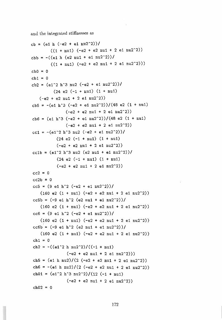
and the integrated stiffnesses as
cb = (el h (-e2 + el nu2-2))/ «1 + nul) (-e2 + e2 nul + 2 el nu2-2))
ebb = -(eel h (e2 nul + el nu2-2))/ «1 + nul) (-e2 + e2 nul + 2 el nu2-2)))
cbO = 0
cbl = 0 cb2 = (el-2 h-3 nu2 (-e2 + el nu2-2))/
(24 e2 (-1 + nul) (1 + nul)
(-e2 + e2 nul + 2 el nu2-2))
cb5 = -eel h-3 (-e2 + el nu2-2))/(48 e2 (1 + nul)
(-e2 + e2 nul + 2 el nu2-2))
cb6 = (el h-3 (-e2 + el nu2-2))/(48 e2 (1 + nul)
(-e2 + e2 nul + 2 el nu2-2))
eel = -(el-2 h-3 nu2 (-e2 + el nu2-2))/
(24 e2 (-1 + nul) (1 + nul)
(-e2 + e2 nul + 2 el nu2-2))
cclb = (el-2 h-3 nu2 (e2 nul + el nu2-2))/
cc2 = 0
cc2b = 0
(24 e2 (-1 + nul) (1 + nul)
(-e2 + e2 nul + 2 el nu2-2))
cc5 = (9 el h-2 (-e2 + el nu2-2))/
(160 e2 (1 + nul) (-e2 + e2 nul + 2 el nu2-2))
cc5b = (-9 el h-2 (e2 nul + el nu2-2))/
(160 e2 (1 + nul) (-e2 + e2 nul + 2 el nu2-2))
cc6 = (9 el h-2 (-e2 + el nu2-2))/
(160 e2 (1 + nul) (-e2 + e2 nul + 2 el nu2-2))
cc6b = (-9 el h-2 (e2 nul + el nu2-2))/
(160 e2 (1 + nul) (-e2 + e2 nul + 2 el nu2-2))
chl = 0
ch2 = -«el-2 h nu2-2)/«-1 + nul)
(-e2 + e2 nul + 2 el nu2-2)))
ch5 = (el h nu2)/(2 (-e2 + e2 nul + 2 el nu2-2))
ch6 = -eel h nu2)/(2 (-e2 + e2 nul + 2 el nu2-2))
chOl = (el-2 h-3 nu2-2)/(12 (-1 + nul)
(-e2 + e2 nul + 2 el nu2-2))
ch02 = 0
172
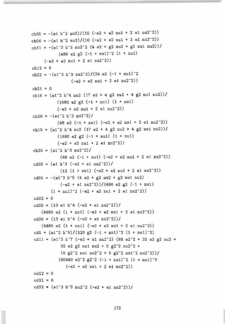
ch05 = -(el h-2 nu2)/(10 (-e2 + e2 nul + 2 el nu2-2))
ch06 = -(el h-2 nu2)/(10 (-e2 + e2 nul + 2 el nu2-2))
chll = -(el-3 h-5 nu2-2 (4 e2 + g2 nu2 + g2 nul nu2))/
(480 e2 g2 (-1 + nul)-2 (1 + nul)
(-e2 + e2 nul + 2 el nu2-2))
ch12 = 0 ch22 = -(el-3 h-3 nu2-3)/(24 e2 (-1 + nul)-2
(-e2 + e2 nul + 2 el nu2-2))
ch21 = 0 ch16 = (el-2 h-4 nu2 (17 e2 + 4 g2 nu2 + 4 g2 nul nu2))/
(1680 e2 g2 (-1 + nul) (1 + nul)
(-e2 + e2 nul + 2 el nu2-2))
ch26 = -(el-2 h-3 nu2-2)/
(48 e2 (-1 + nul) (-e2 + e2 nul + 2 el nu2-2))
ch15 = (el-2 h-4 nu2 (17 e2 + 4 g2 nu2 + 4 g2 nul nu2))/
(1680 e2 g2 (-1 + nul) (1 + nul)
(-e2 + e2 nul + 2 el nu2-2))
ch25 = (el-2 h-3 nu2-2)/
(48 e2 (-1 + nul) (-e2 + e2 nul + 2 el nu2-2))
cdOO = (el h-3 (-e2 + el nu2-2))/
(12 (1 + nul) (-e2 + e2 nul + 2 el nu2-2))
cdOl = -(el-2 h-5 (4 e2 + g2 nu2 + g2 nul nu2) .
(-e2 + el nu2-2))/(480 e2 g2 (-1 + nul)
(1 + nul)-2 (-e2 + e2 nul + 2 el nu2-2))
cd02 = 0
cd05 = (13 el h-4 (-e2 + el nu2-2))/
(4480 e2 (1 + nul) (-e2 + e2 nul + 2 el nu2-2))
cd06 = (13 el h-4 (-e2 + el nu2-2))/
(4480 e2 (1 + nu1) (-e2 + e2 nu1 + 2 e1 nu2-2))
cdl = (e1-2 h-5) / (120 g2 (-1 +. nul) -2 (1 + nul) -2)
cdll = (el-3 h-7 (-e2 + el nu2-2) (68 e2-2 + 32 e2 g2 nu2 +
32 e2 g2 nul nu2 + 5 g2-2 nu2-2 +
cd12 = 0
cd21 = 0
10 g2-2 nu1 nu2-2 + 5 g2-2 nu1-2 nu2-2))/
(80640 e2-2 g2-2 (-1 + nu1)-2 (1 + nu1)-3
(-e2 + e2 nul + 2 el nu2-2))
cd22 = (el-3 h-5 nu2-2 (-e2 + el nu2-2))/
173
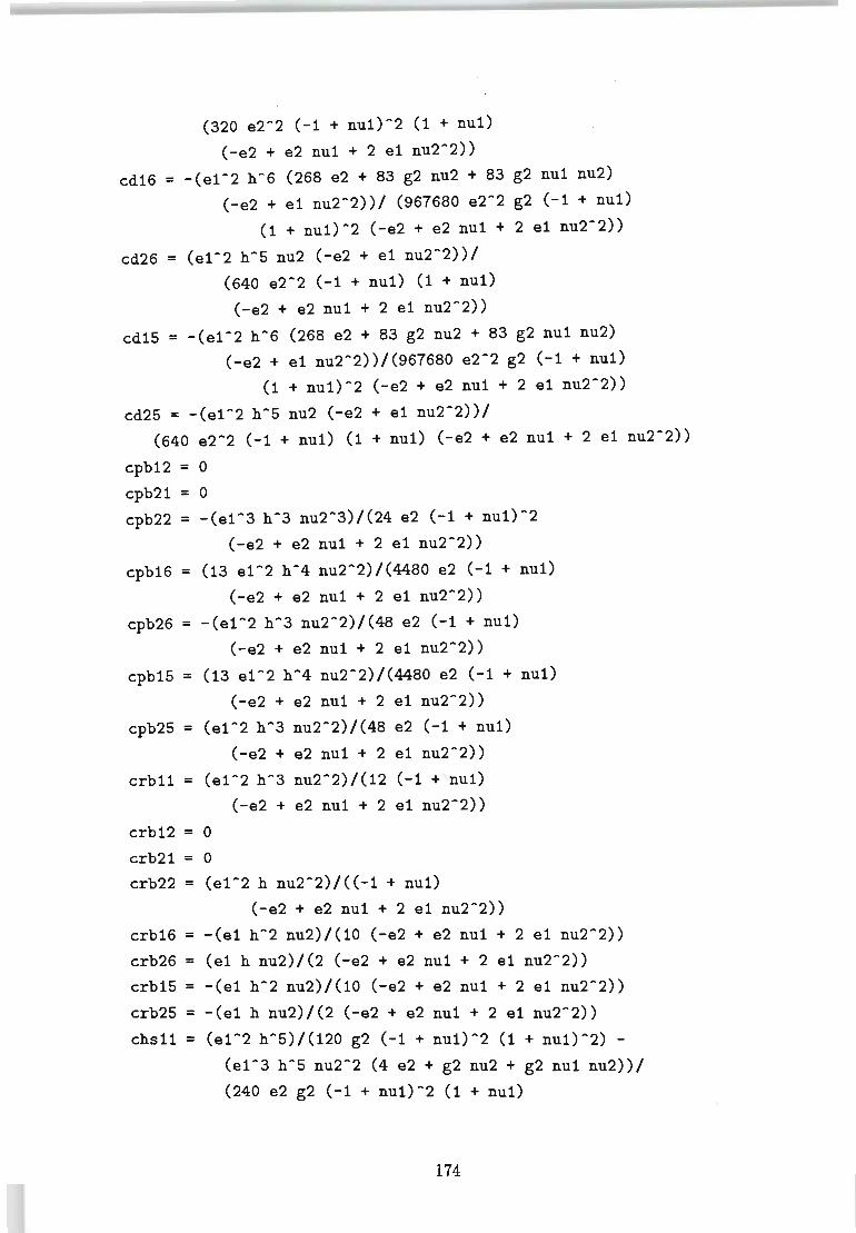
(320 e2-2 (-1 + nul)-2 (1 + nul)
(-e2 + e2 nul + 2 el nu2-2))
cd16 = -(el-2 h-6 (268 e2 + 83 g2 nu2 + 83 g2 nul nu2)
(-e2 + el nu2-2))/ (967680 e2-2 g2 (-1 + nul)
(1 + nul)-2 (-e2 + e2 nul + 2 el nu2-2))
cd26 = (el-2 h-5 nu2 (-e2 + el nu2-2))/
(640 e2-2 (-1 + nul) (1 + nul)
(-e2 + e2 nul + 2 el nu2-2))
cd15 = -(el-2 h-6 (268 e2 + 83 g2 nu2 + 83 g2 nul nu2)
(-e2 + el nu2-2))/(967680 e2-2 g2 (-1 + nul)
(1 + nul)-2 (-e2 + e2 nul + 2 el nu2-2))
cd25 = -(el-2 h-5 nu2 (-e2 + el nu2-2))/
(640 e2-2 (-1 + nul) (1 + nul) (-e2 + e2 nul + 2 el nu2-2))
cpb12 = 0
cpb21 = 0
cpb22 = -(el-3 h-3 nu2-3)/(24 e2 (-1 + nul)-2
(-e2 + e2 nul + 2 el nu2-2))
cpb16 = (13 el-2 h-4 nu2-2)/(4480 e2 (-1 + nul)
(-e2 + e2 nul + 2 el nu2-2))
cpb26 = -(el-2 h-3 nu2-2)/(48 e2 (-1 + nul)
(-e2 + e2 nul + 2 el nu2-2))
cpb15 = (13 el-2 h-4 nu2-2)/(4480 e2 (-1 + nul)
(-e2 + e2 nul + 2 el nu2-2))
cpb25 = (el-2 h-3 nu2-2)/(48 e2 (-1 + nul)
(-e2 + e2 nul + 2 el nu2-2))
crbll = (el-2 h-3 nu2-2)/(12 (-1 + nul)
crb12 = 0
crb21 = 0
(-e2 + e2 nul + 2 el nu2-2))
crb22 = (el-2 h nu2-2)/«-1 + nul)
(-e2 + e2 nul + 2 el nu2-2))
crb16 = -(el h-2 nu2)/(10 (-e2 + e2 nul + 2 el nu2-2))
crb26 = (el h nu2)/(2 (-e2 + e2 nul + 2 el nu2-2))
crb15 = -(el h-2 nu2)/(10 (-e2 + e2 nul + 2 el nu2-2))
crb25 = -(el h nu2)/(2 (-e2 + e2 nul + 2 el nu2-2))
chsll = (el-2 h-5)/(120 g2 (-1 + nul)-2 (1 + nul)-2) -
(el-3 h-5 nu2-2 (4 e2 + g2 nu2 + g2 nul nu2))/
(240 e2 g2 (-1 + nul)-2 (1 + nul)
174
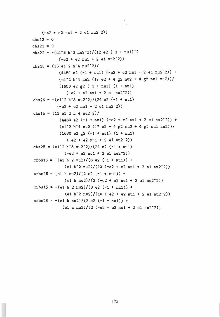
(-e2 + e2 nul + 2 el nu2-2»
chs12 = 0
chs21 = 0 chs22 = -(el-3 h-3 nu2-3)/(i2 e2 (-1 + nul)-2
(-e2 + e2 nul + 2 el nu2-2»
chs16 = (13 el-2 h-4 nu2-2)/
(4480 e2 (-1 + nul) (-e2 + e2 nul + 2 el nu2-2» +
(el-2 h-4 nu2 (17 e2 + 4 g2 nu2 + 4 g2 nul nu2»/
(1680 e2 g2 (-1 + nul) (1 + nul)
(-e2 + e2 nul + 2 el nu2-2»
chs26 = -(el-2 h-3 nu2-2)/(24 e2 (-1 + nul)
(-e2 + e2 nul + 2 el nu2-2»
chs15 = (13 el-2 h-4 nu2-2)/
(4480 e2 (-1 + nul) (-e2 + e2 nul + 2 el nu2-2» +
(el-2 h-4 nu2 (17 e2 + 4 g2 nu2 + 4 g2 nul nu2»/
(1680 e2 g2 (-1 + nul) (1 + nul)
(-e2 + e2 nul + 2 el nu2-2»
chs25 = (el-2 h-3 nu2-2)/(24 e2 (-1 + nul)
(-e2 + e2 nul + 2 el nu2-2»
crbs16 = -(el h-2 nu2)/(8 e2 (-1 + nul» +
(el h-2 nu2)/(10 (-e2 + e2 nul + 2 el nu2-2»
crbs26 = (el h nu2)/(2 e2 (-1 + nul» -
(el h nu2)/(2 (-e2 + e2 nul + 2 el nu2-2»
crbs15 = -(el h-2 nu2)/(8 e2 (-1 + nul» +
(el h-2 nu2)/(10 (-e2 + e2 nul + 2 el nu2-2»
crbs25 = -(el h nu2)/(2 e2 (-1 + nul» +
(el h nu2)/(2 (-e2 + e2 nul + 2 el nu2-2»
175
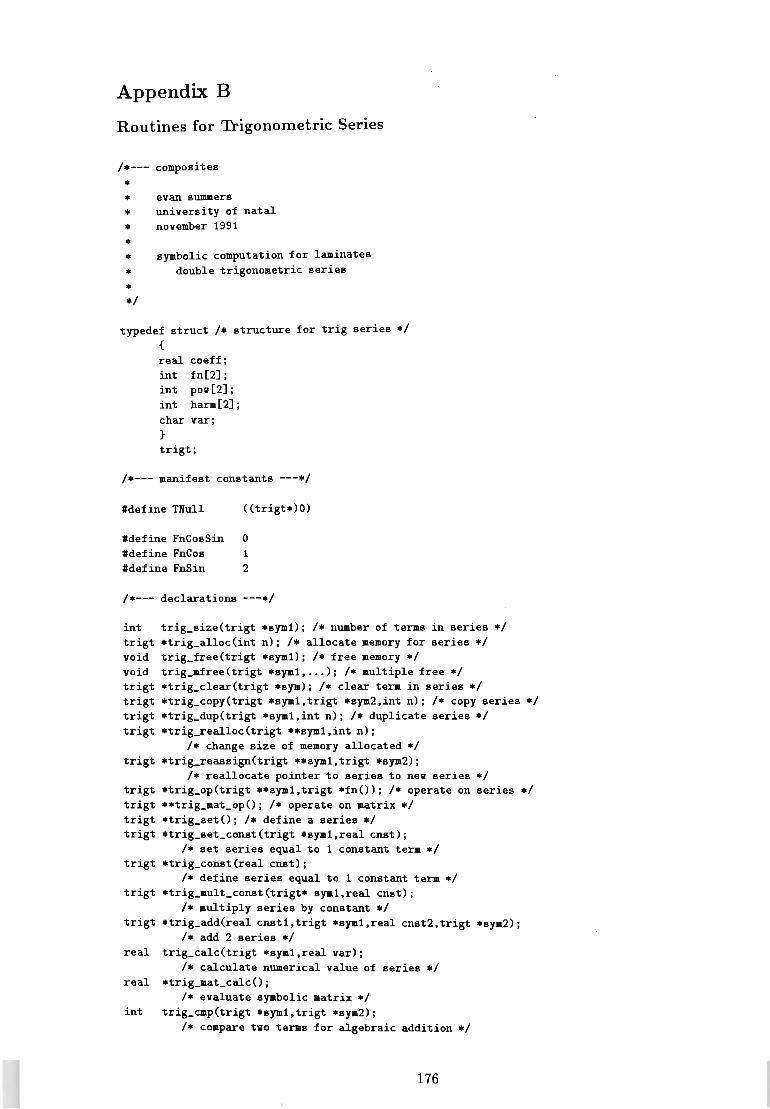
Appendix B
Routines for Trigonometric Series
1*--- composites
* * evan summers * university of natal * november 1991
* * symbolic computat ion for laainates * double trigonometric series
* *1
typedef struct 1* structure for trig series *1 {
real coeff; int fn[2] ; int pov[2] ; int hara[2]; char var; }
trigt;
1*--- manifest constants ---*1
'define THull «trigt*)O)
'define FnCosSin 0 'define FnCos 1 'define FnSin 2
1*--- declarations ---*1
int trigt void void trigt trigt trigt trigt
trigt
trigt trigt trigt trigt
trigt
trigt
trigt
real
real
int
trig_size(trigt *sym1); 1* nuaber of teras in series *1 *trig_alloc(int n); 1* allocate aeaory for series *1 trig_free(trigt *sym1); 1* free aeaory *1 trig_afree(trigt *sya1 •... ); 1* au1tiple free *1 *trig_clear(trigt *sym); 1* clear tera in series *1 *trig_copy(trigt *sya1.trigt *sya2.int n); 1* copy series *1 *trig_dup(trigt *sya1.int n); 1* duplicate series *1 *trig_rea1loc(trigt **sya1.int n);
1* change size of .eaory allocated *1 *trig_reassign(trigt **sym1.trigt *sya2);
/* reallocate pointer to series to nev series */ *trig_op(trigt **sya1.trigt *fn(»; 1* operate on series *1 **tris-aat_op(); 1* operate on aatrix *1 *trig_set(); 1* define a series *1 *trig_set_const(trigt *sya1.real cnst);
1* set series equal to 1 constant tera */ *trig_const(real cnst);
/* define series equal to 1 constant tera *1 *trig_ault_const(trigt* syal.real cnst);
1* aultiply series by constant *1 *trig_add(real cnstl.trigt *syal.real cnst2.trigt *sym2);
1* add 2 series *1 trig_calc(trigt *syal.real var);
1* calculate nuaerical value of series *1 *trig_aat_calc();
1* evaluate syabolic aatrix *1 trig_cap(trigt *syal.trigt *sya2);
1* co.pare tvo teras for algebraic addition *1
176
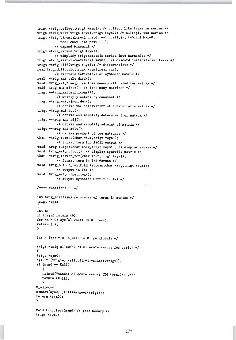
trigt *trig_collect(trigt *syml); /* collect like terms in series */ trigt *trig_mult(trigt *syml.trigt *sym2); /* multiply tvo series */ trigt *trig_binomial(real cnstO.real coeff.int fnO.int harmO •.
real cnstl . int povO •... ); /* expand binomial */
trigt *trig_expand(trigt *syml); /* simplify trigonometric series into harmonics */
trigt *trig_significant(trigt *syml); /* discard insignificant terms */ trigt *trig_diff(trigt *syml); /* differentiate */ real trig_diff_calc(trigt *syml.real var);
/* evaluate derivative of symbolic matrix */ real *trig_mat_calc_diff(); void trig_mat_free(); /* free memory allocated for matrix */ void trig_mat_mfree(); /* free many matrices */ trigt **trig_mat_mult_const();
/* multiply matrix by constant */ trigt *trig_mat_minor_det();
/* derive the determinant of a minor of a matrix */ trigt *trig_mat_det();
/* derive and simplify determinant of matrix */ trigt **trig_mat_adj();
/* derive and simplify adjoint of matrix */ trigt **trig_mat_mult();
/* derive product of tvo matrices */ char *trig_format(char *buf.trigt *syml);
/* format term for ASCII output */ void trig_output(char *msg.trigt *syal); /* display series */ void trig_aat_output(); /* display symbolic matrix */ char *trig_format_tex(char *buf.trigt *syml);
/* format term in TeX format */ void trig_output_tex(FlLE *stream.char *msg.trigt *syml);
/* output in TeX */ void trig_mat_output_tex();
/* output symbolic matrix in TeX */
int trig_size(sym) /* number of teras in series */ trigt *sym; {
int n; if (!sym) return (0); for (n - 0; sym[n].coeff !- 0.; n++); return (n); }
int n_free - O. n_alloc - 0; /* globals */
trigt *trig_alloc(n) /* allocate memory for series */ {
trigt *syaO; symO - (trigt*) malloc«n+l)*sizeof(trigt»; if (symO -- Null)
{
printf("cannot allocate memory (~d teras)\n".n); return (Null); }
n_alloc++; memset(symO.O.(n+l)*sizeof(trigt»; return (syaO); }
void trig_free(symO) /* free memory */ trigt *syaO;
177
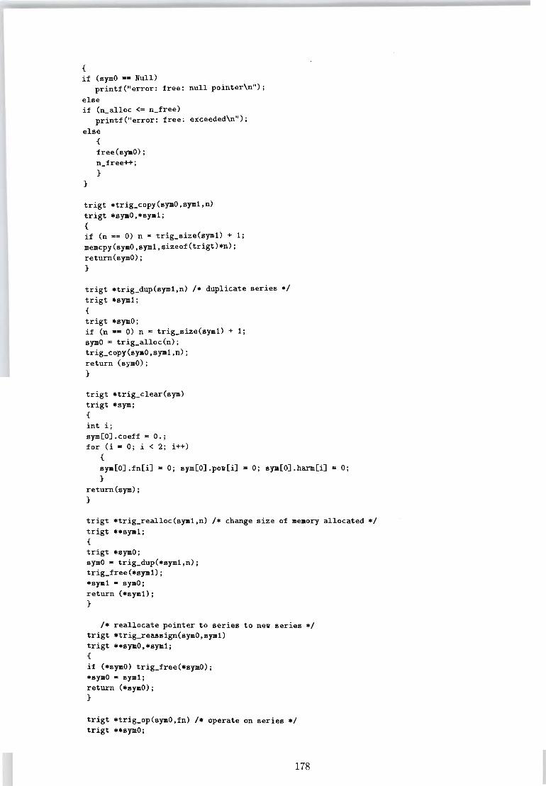
{
if (syaO .- Hull) printf("error: free: null pointer\n");
else if (n_alloc <- n_free)
printf("error: free: exceeded\n"); else
}
{
free(syaO); n_free++; }
trigt .trig_copy(syaO,syal,n) trigt .syaO,.syal; {
if (n -= 0) n - trig_size(sym1) + 1; aemcpy(syaO,sya1,sizeof(trigt)*n); return(syaO) ; }
trigt .trig_dup(sya1,n) /. duplicate series ./ trigt .sya1; {
trigt .syaO; if (n .- 0) n • trig_size(sya1) + 1; syaO - trig_alloc(n); trig_copy(syaO,sya1,n); return (symO); }
trigt .trig_clear(sym) trigt .sya; {
int i; sya[O] . coeff • 0.; for (i • 0; i < 2; i++)
{
sya[O].fn[i] - 0; sya[O].pow[i] - 0; sya[O].harm[i] 0; }
return(sya) ; }
trigt .trig_realloc(sya1,n) /. change s i ze of .e.ory allocated ./ trigt "sya1; {
trigt .syaO; syaO· trig_dup(.sya1,n); trig_free(.sya1); .sya1 • syaO; return (.sya1); }
/. reallocate pointer to series to new series ./ trigt .trig_reassign(syaO,sya1) trigt •• syaO,.syal; {
if (.syaO) trig_free(.syaO); .syaO - syal; return (.syaO); }
trigt .trig_op(syaO,fn) /. operate on series ./ trigt .. syaO;
178
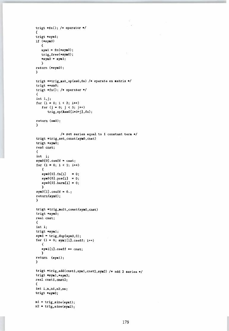
trigt *fn(); /* operator */ {
trigt *syml; if (*symO)
{
syml - fn(*symO); trig_free(*symO); *symO - syml; }
return (*symO); }
trigt **trig_lIlat_op(sIllO,fn) /* operate on matrix */ trigt **SIllO; trigt *fn(); /* operator */ {
int i,j; for (i - 0; i < 3; i++)
for (j - 0; j < 3; j++) trig_op(lsIll0[i*3+j),fn);
return (SIllO); }
/* set series equal to 1 constant term */ trigt *trig_set_const(symO,cnst) trigt *symO; real cnst; {
int i; syaO[O).coeff - cnst; for (i - 0; i < 2; i++)
{
syaO[O) .fn[i) - 0; symO[O).pov[i) = 0; symO[O).harm[i) - 0; }
symO[1).coeff - 0.; return(s)'1l0) ; }
trigt *trig_lIIult_const(symO,cnst) trigt *syaO; real cnst; {
int i; trigt *syal; sya1 - trig_dup(symO,O); for (i - 0; sya1[i).coeff; i++)
{
syml[i).coeff *- cnst; }
return (s)'1l1) ; }
trigt *trig_add(cnst1,sym1,cnst2,sya2) /* add 2 series */ trigt *sya1,*sya2; real cnst1,cnst2; {
int i,n,n1,n2,ns; trigt *syaO;
n1 - trig_size(sym1); n2 - trig_size(sya2);
179
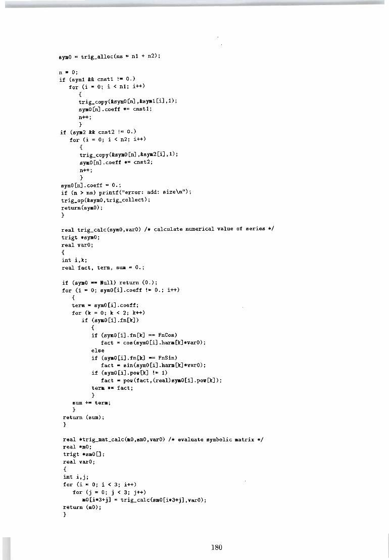
symO - trig_alloc(ns - n1 + n2);
n - 0; if (sym1 tt cnst1 !- 0 . )
for (i - 0; i < n1; i++) { trig_copy(tsymO[n] ,tsym1[i] ,1); symO[n].coeff *= cnst1; n++; }
if (sym2 tt cnst2 !- 0.) for (i - 0; i < n2; i++)
{
trig_copy(tsymO[n] ,tsym2[i] ,1); symO[n].coeff *= cnst2; n++; }
symO[n].coeff - 0.; if (n > ns) printf("error: add: size\n"); trig_op(tsymO,tris-collect); return(symO) : }
real trig_calc(symO,varO) /* calculate numerical value of series */ trigt *symO: real varO: {
int i,k; real fact, term, sum - 0.;
if (symO -- Null) return (0.): for (i - 0; syaO[i].coeff !- 0.; i++)
{
term - symO[i].coeff; for (k - 0: k < 2; k++)
if (symO[i].fn[k]) {
if (symO[i].fn[k] -= FnCos) fact - cos(symO[i].harm[k]*varO);
else if (symO[i].fn[k] -- FnSin)
fact - sin(symO[i].harm[k]*varO); if (symO[i] .POll[k] !- 1)
fact - pOll(fact,(real)symO[i].poll[k]); term *- fact; }
SUII +- tena: }
return (sum); }
real *trig_aat_calc(mO,saO,varO) /* evaluate symbolic matrix */ real *aO; trigt *saO[]: real varO: {
int i,j; for (i - 0; i < 3; i++)
for (j - 0: j < 3; j++) aO[i*3+j] - trig_calc(smO[i*3+j],varO);
return (aO): }
180
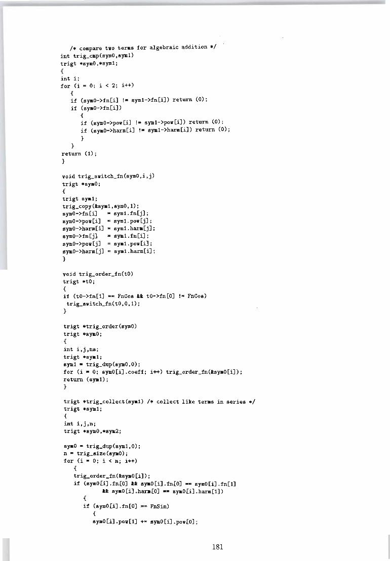
/* compare tvo teras for algebraic addition */ int trig_cmp(syaO,sym1) trigt *symO,*sya1; { int i; for (i - 0; i < 2; i++)
{ if (symO->fn[i] !- sym1->fn[i]) return (0); if (symO->fn[i])
{ if (symO->pov[i] !- sym1->pov[i]) return (0); if (symO->harm[i] !- sym1->harm[i]) return (0); }
} return (1); }
void trig_svitch_fn(symO,i,j) trigt *symO; { trigt sym1; trig_copy(1sym1,symO, 1); symO->fn[i] - sym1.fn[j]; symO->pov[i] - sym1.pov[j]; symO->harm[i] - sym1.harm[j]; symO->fn[j] - sym1.fn[i]; symO->pov[j] - sym1.pov[i]; symO->harm[j] x sym1.harm[i]; }
void trig_order_fn(tO) trigt *to; { if (to->fn[l] -- FnCos 11 to->fn[O] !- FnCos) trig_svitc~fn(tO,O,l);
}
trigt *trig_order(symO) trigt *symO; { int i,j,ns; trigt *sya1; sya1 - trig_dup(symO,O); for (i - 0; syaO[i].coeff; i++) trig_order_fn(1syaO[i]); return (aya1); }
trigt *trig_collect(sya1) /* collect like teras in series */ trigt *sya1; { int i,j,n; trigt *syaO,*sya2;
syaO - trig_dup(sya1,O); n· trig_size(syaO); for (i - 0; i < n; i++)
{ trig_order_fn(1syaO[i]); if (symO[i].fn[O] 11 syaO[i].fn[O] -- syaO[i].fn[l]
11 syaO[i].hara[O] -- syaO[i].hara[l]) { if (syaO[i].fn[O] _x FnSin)
{ syaO[i].pov[l] +- symO[i].pov[O];
181
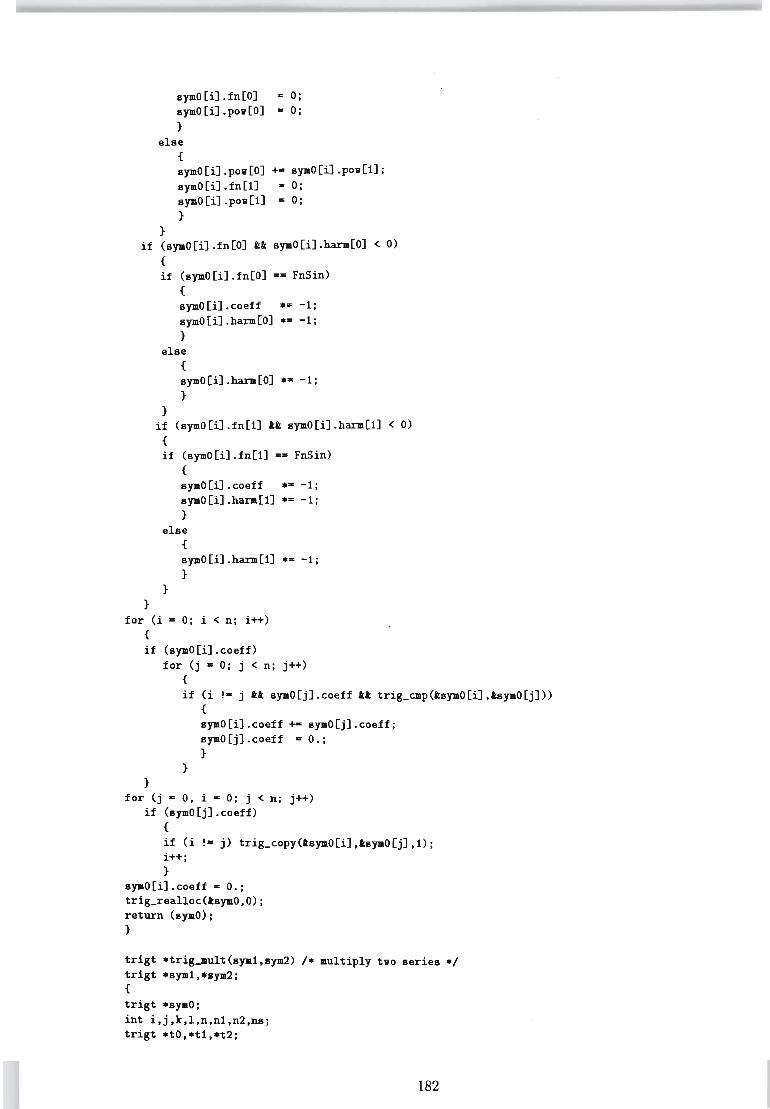
symO[i).fn[O] - 0; symO[i).pov[O) - 0; }
else
}
{ symO[i).pov[O) += symO[i).pov[1); symO[i).fn[1) - 0; symO[i).pov[1) - 0; }
if (syaO[i).fn[O) 11 symO[i).hara[O) < 0) {
}
if (symO[i).fn[O) -= FnSin) { symO[i).coeff *- -1; symO[i).harm[O) *= -1; }
else
}
{ symO[i).hara[O) *= -1; }
if (symO[i).fn[1) 11 symO[i).hara[1) < 0) { if (symO[i).fn[1) -- FnSin)
{ symO[i).coeff *= -1; symO[i).harm[1) *= -1; }
else
}
{ syaO[i).hara[1) *- -1; }
for (i = 0; i < n; i++) { if (symO[i).coeff)
for (j • 0; j < n; j++) { if (i !- j 11 syaO[j).coeff 11 trig_cap(lsyaO[i),lsyaO[j))
{
} }
syaO[i).coeff +- syaO[j).coeff; syaO[j).coeff - 0.; }
for (j - 0, i - 0; j < n; j++) if (syaO[j).coeff)
{ if (i !- j) trig_copy(lsyaO[i),lsyaO[j),1);
} syaO[i).coeff - 0.; trig_realloc(lsyaO,O); return (syaO); }
trigt *trig_ault(sya1,sya2) /* aultiply tvo series */ trigt *sya1,*sya2; { trigt *syaO; int i,j,k,1,n,n1,n2,ns; trigt *to,*t1,*t2;
182
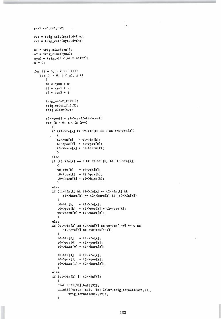
real rvO,rvl,rv2;
rvl - trig_calc(syml,dvthe)j rv2 - trig_calc(sym2,dvthe);
nl - trig_size(syml); n2 - trig_size(sym2); symO = trig_alloc(ns = nl*n2); n - 0;
for (i - 0; i < nl; i++) for (j - 0; j < n2; j++)
{
to - symO + n; tl - syml + i; t2 - sym2 + j;
trig_order_fn(tl); trig_order_fn(t2); trig_clear(tO);
to->coeff = tl->coeff*t2->coeff; for (k - 0; k < 2; k++)
{
if (tl->fn[k] tt t2->fn[k] -- 0 tt !to->fn[k]) {
to->fn[k] - tl->fn[k]; to->pov[k] - tl->pov[k]; to->harm[k] - tl->harm[k]; }
else if (tl->fn[k] -= 0 tt t2->fn[k] tt !to->fn[k])
{
to->fn[k] = t2->fn[k]; to->pov[k) • t2->pov[k]; to->hara[k] - t2->hara[k]; }
else if (tl->fn[k] tt tl->fn[k] -= t2->fn[k] tt
tl->harm[k] _. t2->harm[k] tt !to->fn[k]) {
to->fn[k] = tl->fn[k]; to->pov[k] • tl->pov[k) + t2->pov[k]; to->hara[k] - tl->hara[k]; }
else if (tl->fn[k] tt t2->fn[k] tt to->fn[l-k] -= 0 tt
!to->fn[k] tt !to->fn[l-k]) {
to->fn[O] • tl->fn[k]; to->pov[O] • tl->pov[k]j to->hara[O] - tl->harm[k];
to->fn[l] - t2->fn[k]; to->pov[l] = t2->pov[k]; to->hara[l] - t2->hara[k); }
else if (tl->fn[k] I I t2->fn[k)
{
char bufl(32),buf2[32]; printf("error: ault: Xs: Xs\n", trig_format(bufl, to,
trig_format(buf2,t2»; }
183
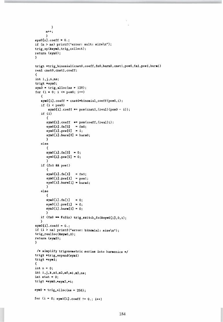
}
n++; }
symO[n].coeff - 0.; if (n > ns) printf("error: mult: size\n"); trig_op(tsymO,trig_collect); return (symO); }
trigt *trig_binomial(cnstO,coeff,fnO,harmO,cnst1,powO,fn1,pow1,harm1) real cnstO,cnst1,coeff; {
int i,j,n,ns; trigt *symO; symO - trig_alloc(ns· 128); for (i - 0; i <- powO; i++)
{
symO[i].coeff - cnstO*binomial_coeff(powO,i); if (i < powO)
syaO[i].coeff *- pow(cnst1,(real)(powO - i»; if (i)
{
symO[i].coeff *- pow(coeff,(real)i); symO[i].fn[O] - fnO; symO[i] .pow[O] - i; symO[i].harm[O] - harmO; }
else {
symO[i] .fn[O] • 0; symO[i].pow[O] - 0; }
if (fn1 11 pow1) {
symO[i].fn[1] - fn1; symO[i].pow[1] - pow1; symO[i].harm[1] - hara1; }
else {
symO[i].fn[1] - 0; symO[i].pow[1] - 0; symO[i] . hara[1] - 0; }
if (fnO -- FnSin) trig_switch_fn(lsyaO[i],O,1); }
syaO[i].coeff - 0.; if (i > ns) printf("error: binomial: size\n"); trig_realloc(lsyaO,O); return (syaO); }
/* simplify trigonometric series into haraonics */ trigt *trig_expand(sya1) trigt *sya1; {
int n - 0; int i,j,k,n1,n2,mO,m1,m2,ns; int stat - 0; trigt *syaO,*sya2,*t;
symO - trig_alloc(ns - 256);
for (i - 0; sya1[i].coeff !- 0.; i++)
184
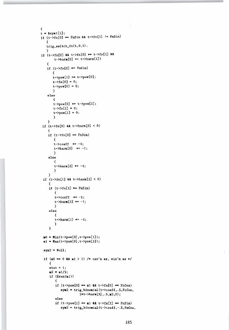
{
t - &:sy.1 [i] ; if (t->fn[O] -- FnSin 11 t->fn[l] !- FnSin)
{ trig_svitch_fn(t,O,l); }
if (t->fn[O] 11 t->fn[O] _s t->fn[l] 11 t->hara[O] -- t->hara[l])
{
if (t->fn[O] -- FnSin) {
t->pov[l] +- t->pov[O]; t->fn[O] - 0; t->pov[O] .. 0; }
else
}
{
t->pov[O] +- t->pov[l]; t->fn[1] - 0; t->pov[l] .. 0; }
if (t->fn[O] 11 t->hara[O] < 0) {
if (t->fn[O] -- FnSin) {
t->coeff .- -1; t->hara[O] .- -1; }
else
}
{
t->hara[O] .- -1; }
if (t->fn[l] 11 t->hara[l] < 0) {
if (t->fn[l] -- FnSin) {
t->coeff .- -1; t->hara[l] ... -1; }
else
}
{
t->hara[l] ... -1; }
aO - Min(t->pov[0],t->pov[1]); a1 - Max(t->pov[0],t->pov[1]);
sya2 - Hull;
if (aO -- 0 11 a1 > 1) /. cos·n ax, sin·n ax ./ {
stat .. 1; a2 .. a1/2; if (Even(aO)
{
if (t->pov[O] -- a1 11 t->fn[O] -- FnCos) sya2 - trig_binoaial(t->coeff,.5,FnCos,
2.t->hara[0], . 5,a2,O); elae if (t->pov[1] -- a1 11 t->fn[l] -- FnSin)
aya2 - trig_binoaial(t->coeff,-.5,FnCos,
185
. 2*t->hara[1],.5,m2,O); else
printf (llerror: expand: %s\n" ,trig_format (bufO, t»; }
else {
if (t->pov[O] _ .. m1 tt t->fn[O] -= FnCos) sym2 - trig_binomial(t->coeff,.5,FnCos,
2*t->harm[0] , . 5,m2,t->fn[0],l,t->hara[0]);
else if (t->pov[l] -- a1 tt t->fn[l] _. FnSin)
sym2 - trig_binomial(t->coeff,-.5,FnCos, 2*t->hara[1] , .5,m2,t->fn[1],l,t->hara[1]);
else printf("error: expand: %s\n" ,trig_format(bufO,t»;
}
}
else if (t->fn[O] -- FnCos tt t->fn[l] -= FnSin
tt t->hara[O] -- t->hara[l] tt t->pov[O] -= t->pov[l]) {
stat - 2; symO [n] . coeti symO[n] .fn[O] symO[n] .pov[O] symO [n] . fn[l] symO [n] . pov [1]
symO[n] .harm[1]
- pov(.5,(real)aO)*t->coeff;
n++; }
else
.. 0;
- 0; .. FnSin; '" t->pov [0] ; - 2*t->harm[0];
if (t->fn[O] -- FnCos tt t->fn[l] -- FnSin tt t->hara[O] -= t->hara[1] tt Even(a1 - mO» {
stat - 3; a2 - (m1 - aO)/2; if (t->pov[O] _. aO)
{
sym2 - trig_binomial(pov(.5,(real)aO)*t->coeff, -.5,FnCos,2*t->harm[0],.5,m2,FnSin, mO,2*t->hara[0]);
}
else {
sym2 - trig_binoaial(pov(.5,(real)aO)*t->coeff, .5,FnCos,2*t->hara[0),.5,a2,FnSin, aO,2*t->hara[0]);
}
}
else if (mO tt Even(m1»
{
stat - 4; a2 - a1/2; if (m1 -- t->pov[O])
{
if (t->fn[O] -- FnCos) sym2 - trig_binomial(t->coeff,.5,FnCos,2*t->hara[0],
.5,a2,t->fn[1],t->pov[1],t->hara[1]); else if (t->fn[O] -- FnSin)
sya2 - trig_binoaial(t->coeff,-.5,FnCos,2*t->hara[0],
186
.S,a2,t->fn[1],t->pov[1],t->harm[1]): }
e18e if (a1 -- t->pov[l])
{
}
else
if (t->fn[l] -- FnCo8) 8ym2 ~ trig_binoaial(t->coeff,.S,FnCos,2*t->harm[1],
.S,a2,t->fn[0],t->pov[0],t->harm[0]): else if (t->fn[l] -- FnSin)
}
sym2 - trig_binoaial(t->coeff,-.S,FnCos,2*t->hara[1], .S,a2,t->fn[0],t->pov[0],t->hara[0]):
if (t->pov[O] -= 1 tt t->pov[l] -= 1) {
stat - S: if (t->fn[O] -- FnSin tt t->fn[l] -- FnCos)
{
symO[n].coeff - .S*t->coeff: symO[n) .fn[O] • 0: 8ymO[n) .pov[O] - 0: 8yaO[n) .fn[l] - FnSin: syaO[n] .pov[l] - 1: syaO[n].hara[l] - t->hara[O] - t->hara[l]: n++: symO[n].coeff - .S*t->coeff: syaO[n] .fn[O] - 0: syaO[n] .pov[O] - 0: symO[n] .fn[l] ~ FnSin: syaO[n) .pov[l] - 1: 8ymO[n).hara[1] - t->harm[l] + t->hara[O]: n++: }
else if (t->fn[O] -- FnCos tt t->fn[l] -- FnSin)
{
- .S*t->coeff: - 0: - 0: - FnSin: • 1:
syaO [n] . coeff syaO[n] .fn[O] syaO[n] .pov[O] 8yaO[n) .fn[l] 8yaO[n] .pov[l] syaO[nJ . hara [1] n++:
- t->harm[l] - t->hara[O]:
- .S*t->coeff; • 0: - 0: - FnSin: - 1:
8yaO [n) . coeff 8yaO[n] .fn[O] 8yaO[n) .pov[O] 8yaO[n] .fn[1] ayaO[nJ .pov[l] 8yaO[n] .hara[1] - t->hara[l] + t->hara[O]: n++: }
e18e if (t->fn[O] -- FnCos tt t->fn[l] -- FnCos)
{
8yaO[n).coeff •. S*t->coeff: 8yaO[n) .fn[O] - FnCo8: 8yaO[n) .pov[O] • 1: 8yaO[n).hara[O] - ab8(t->harm[1] - t->hara[O]); 8yaO[n) .fn[l] - 0: 8yaO[nJ .pov[l] • 0: n++: 8yaO[n).coeff - .S*t->coeff:
187
ayaO[n) .fn[O] • FnCoaj ayaO[n) .pov[O] - 1j ayaO[n).hara[O] • t->hara[1] + t->hara[O]j ayaO[n) .fn[1] • OJ aymO[n) .pov[1] '" OJ n++j }
else if (t->fn[O] .'" FnSin 1t t->fn[1] •• FnSin)
{ ayaO[n).coeff •• S*t->coeffj a}'llO[n) .fn[O] • FnCoaj ayaO[n) .pov[O] • 1j ayaO[nJ .hara[O] • aba(t->hara[1] - t->hara[O]) j ayaO [n] . fn[1] • 0 j ayaO[n) .pov[1] • OJ n++j ayaO[n).coeff '" -.S*t->coeffj aymO [n) • fn[O] '" FnCos j s}'110 [n) . pov [0] • 1 j a}'llO[n).harm[O] • t->harm[1] + t->harm[O]j symO[n) .fn[1] • OJ symO[n] .pov[1] • OJ n++j }
else printf(lterror: expand\nlt)j
}
else if (t->fn[O] .- FnCos 11 t->fn[1] .- FnSin
11 t->hara[O] .- t->hara[1]) {
stat· 6j
S}'llO[n).coeff • pov(.S,(real).O)*t->coeffj
if (t->pov[O] .- .0) {
ayaO[n) .fn[O] • FnSinj ayaO[n) .pov[O] •• OJ ayaO [nJ .hara[O] • 2*t->hara[0] j syaO[n).pov[1] -•• OJ }
else {
ayaO[n).pov[O] -- .OJ syaO[n] .fn[l] • FnSinj ayaO[n) .pov[1] •• OJ ayaO[n).hara[1] .2*t->hara[O]j }
n++j }
else {
trig_copy(1syaO[n),1aya1[i],1)j n++j }
if (sya2) {
n1 - trig_aize(aya2)j
if (n+n1 > ns - 64)
188
{
trig_realloc(lsymO,ns +- 32); }
trig_copy(lsymO[nJ,sym2,nl); trig_free(sym2); n +- nl; }
else if (n > ns - 64)
{
trig_realloc(lsymO,ns +- 32); }
}
symO[n].coeff - 0.;
trig_op(lsymO,trig_collect); if (stat) trig_op(lsymO,trig_expand); return (symO); }
trigt *trig_significant(syml) /* discard insignificant terms */ trigt *syml; {
int i,j,n; trigt *symO; real rll. - 0.;
symO - trig_dup(syml,O);
n" trig_size(symO);
for (i - 0; i < n; i++) if (fabs(symO[i].coeff) > rm)
rm - fabs(symO[i] . coeff);
for (i - 0; i < n; i++) if (fabs(symO[i].coeff/rm) < dvsig)
symO[i].coeff - 0.;
i .. 0;
for (j - 0; j < n; j++) if (symO[j].coeff)
{
if (i !- j) trig_copy(lsymO[i],tsymO[j],l) ; i++; }
symO[i].coeff .. 0.;
trig_realloc(lsymO,O);
return (symO); }
trigt *trig_diff(tl) /* differentiate */ trigt *tl; {
int i,k,nl,n - O,ns; trigt *to; real rvO,rvl;
nl - trig_size(tl); to - trig_alloc(ns - nl*2);
189
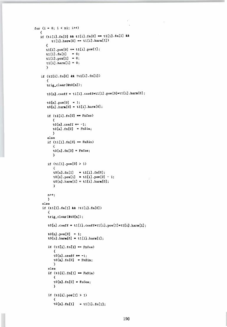
for (i - 0: i < n1: i++) { if (t1[i).fn[0) 11 t1[i).fn[0) -- t1[i).fn[1) 11
t 1[i) .harm[O) -- t 1[i) . harm [1) ) {
t1[i).pov[0) +- t1[i).pov[1): t1[iJ .fn[1) - 0: t1[i).pov[1) - 0: t1 [i) .hara[1) - 0: }
if (t1[i).fn[0) 11 !t1[i).fn[1) {
trig_clear(ltO[n):
to[n).coeff - t1[i).coeff*t1[i).pov[0)*t1[i).harm[0):
to[n).pov[O) - 1: to[n) .hara[O) - t1[i) .hara[O):
if (t1[i).fn[0) -- FnCos) {
to[n).coeff *E -1: to[n).fn[O) - FnSin: }
else if (t1[i).fn[0) -- FnSin)
{
to[n] .fn[O) - FnCos: }
if (t1[i).pov[0) > 1) {
to[n).fn[1) - t1[i).fn[0): to[n) .pov[1) - t1[i) .pov[O) - 1: to[n).hara[1) ~ t1[i).harm[0): }
n++: }
else if (t1[i) .fn[1) tt !t1[i) .fn[O)
{
trig_clear(1tO[n):
to[n).coeff - t1[i).coeff*t1[i).pov[1)*t1[i).hara[1):
to[n] .pov[O) - 1: to[n) .hara[O) - t1[i) .hara[1):
if (t1[i).fn[1) -- FnCos) {
to En) .coeff *- -1: to[n).fn[O) - FnSin; }
else if (t1[i).fn[1) -- FnSin)
{
to[n].fn[O) - FnCos; }
if (t1[i) .pov[1) > 1) {
to[n) .fn[1) - t1[i].fn[1):
190
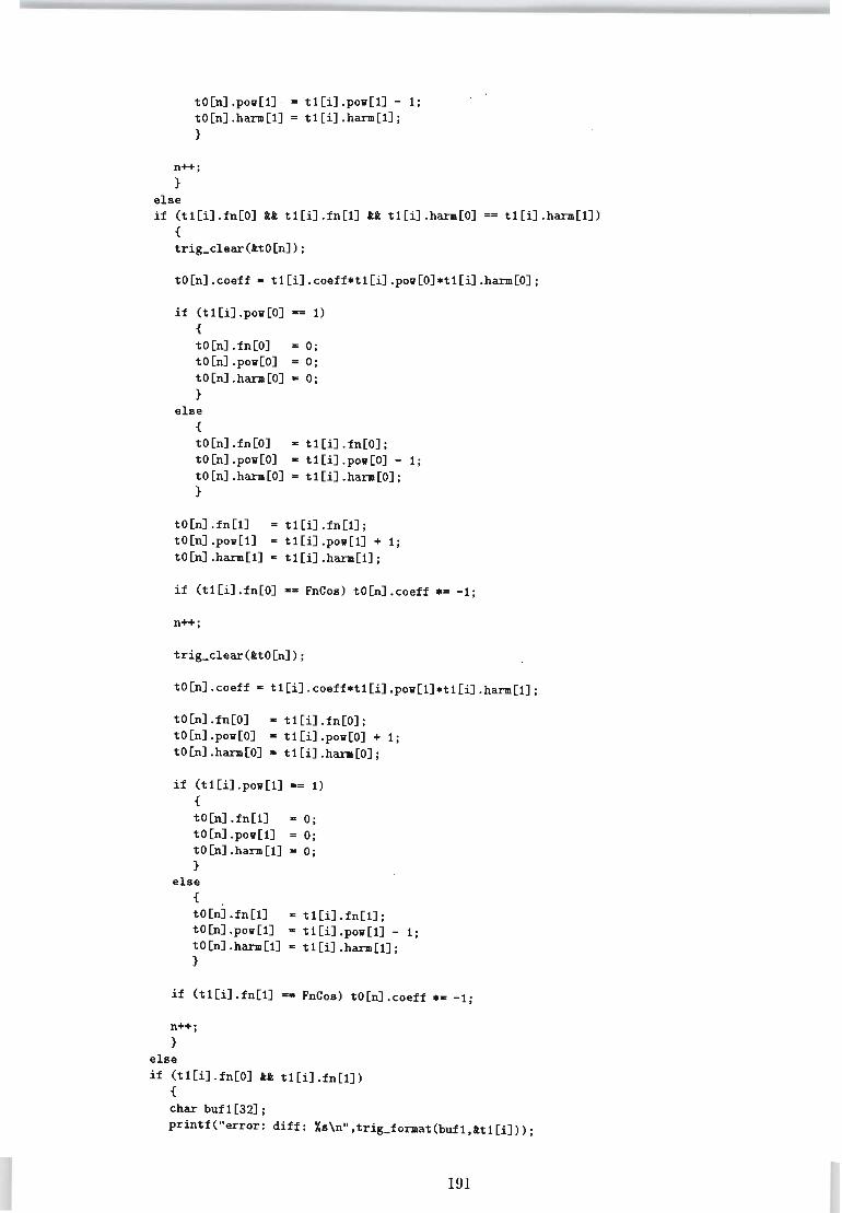
to[n] .pOll[1] · .. t1[i] . pOll [1] - 1; to[n] .harm[l] .. t1[i] .harm[l]; }
n++; }
else if (t1[i].fn[0] tt t1[i].fn[1] tt t1[i].harm[0] == t1[i].harm[1])
{
trig_clear(ltO[n]);
to[n].coeff" t1[i].coeff*t1[i].pOll[0]*t1[i].harm[0];
if (t1[i].pOll[0] -= 1) {
to[n] .fn[O] .. 0; to[n] .pOll[O] .. 0; to [n] • harm [0] .. 0; }
else {
to[n] .fn[O] .. t 1[i] . fn[O] ; to[n] .POll[O] .. t 1[i] . pOll [0] -to[n] .harm[O] .. t1[i] .harm[0]; }
to[n].fn[l] .. t1[i].fn[l]; to[n].poll[l] .. t1[i].pOll[1] + 1; to[n] .harm[l] .. t1[i] . harm [1] ;
1 ;
if (t1[i].fn[0] _ .. FnCos) to[n].coeff * .. - 1;
n++;
trig_clear(ttO[n]);
to[n].coeff - t1[i] . coeff*t1[i].poll[1]*t1[i] .harm[1];
to[n].fn[O] - t1[i].fn[O]; to[n].poll[O] .. t1[i].pOll[0] + 1; to[n] .harm[O] .. t1[i] . harm [0] ;
if (t1 [i] . pOll [1] -= 1) {
to[n] .fn[l] .. 0; to[n].poll[l] .. 0; to[n).harm[l) .. 0; }
else {
to[n).fn[l) - t1[i).fn[1); to[n) .poll[l) - t1[i] .poll[l) - 1; to[n) .harm[l) - t1[i) • harm [1] ; }
if (t1[i].fn[1] .- FnCos) to[n].coeff * .. -1;
n++; }
else if (t1[i].fn[0] tt t1[i] . fn[1])
{
char bufl [32] ; printf("error: diff: Xs\n",trig_foraat(buf1,lt1[i]»;
191
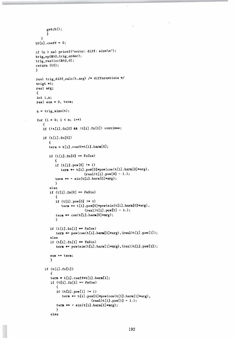
getchO; }
}
to[n].coeff - 0;
if (n > ns) printf("error: diff: size\n"); trig_op(ttO,trig_order); trig_realloc(ttO,O); return (to); }
real trig_diff_calc(t,arg) /* differentiate */ trigt *t; real arg; {
int i,n; real sua - 0, term;
for (i - 0; i < n; i++) {
if (!t[i].fn[O] tt !t[i].fn[1]) continue;
if (t[i] .fn[O]) {
term - t[i].coeff*t[i].harm[O];
if (t[i] .fn[O] _ .. FnCos) {
if (t[i] • pOll [0] != 1) term *- t[i].pOll[O]*POll(COS(t[i].harm[O]*arg),
(real)t[i].pOll[O] - 1.); term *- - sin(t[i].harm[O]*arg); }
else if (t[i].fn[O] -- FnSin)
{
if (t[i].pOll[O] !- 1) term *- t[i].pOll[O]*POll(sin(t[i].harm[O]*arg),
(real)t[i].pOll[O] - 1.); tera *- cos(t[i].harm[O]*arg); }
if (t[i].fn[1] -- FnCos) tera *- pOll(cos(t[i].hara[1]*arg),(real)t[i].pOll[1]);
else if (t[i].fn[1] -- FnSin)
term *- pOll (s in ( t [i] . harm [1] *arg) , (real)t [i] . pOll [1] ) ;
SUIII +a term; }
if (t [i] .fn[1]) {
tera - t[i].coeff*t[i].harm[1]; if (t[i].fn[1] a- FnCos)
{
if (t[i] .poll[1] !- 1) term *- t[i].pOll[1]*POll(COS(t[i].harm[1]*arg),
(real)t [i] .poll[1] - 1.); term * .. - sin(t[i].harm[1]*arg); }
else
192

if (t[i].fn[l] _. FnSin) {
if (t[i].pow[l] !- 1) tera *= t[i].pow[l]*pow(sin(t[i].harm[l]*arg),
(real)t [i] .pow[l] - 1.);
term *. cos(t[i].harm[l]*arg); }
if (t[i].fn[O] -= FnCos) tera *- pow(cos(t[i].harm[O]*arg),(real)t[i].pow[O]);
else if (t[i].fn[O] == FnSin)
term *= pow(sin(t [i] . harm [0] *arg) , (real)t [i] .pow [0]) ;
SUIII += term; }
}
return (SUIII);
}
/*--- aatrices ---*/
/* multiply matrix by constant */ trigt **trig_mat_mult_const(sm,cnst) trigt *sm [] ; real cnst; {
int i,j,n;
for (i = 0; i < 3; i++) for (j - 0; j < 3; j++)
for (n - 0; sll[i*3+j] [n] .coeff !- 0 . ; n++) sm[i*3+j][n].coeff *- cnst;
return (Sll); }
/* derive the determinant of a minor of a aatrix */ trigt *trig_mat_minor_det(smO,i,j) trigt *smO [] ; {
int al,m2,nl,n2; trigt *symO,*syml,*sym2;
al - (i+l)X3j nl - (j+l)X3j a2 - (i+2)X3; n2 - (j+2)X3;
syml - trig_ault(saO[al*3+nl],smO[m2*3+n2]); sym2 - trig_ault(smO[m2*3+nl],smO[ml*3+n2]) j
symO - trig_add(1.,syml,-1.,sym2); trig_free(syal); trig_free(sym2);
trig_op(lsymO,trig_collect);
return (syaO); }
/* derive and siaplify determinant of aatrix */ trigt *trig_aat_det(smO) trigt *smO [] ; {
int i;
193
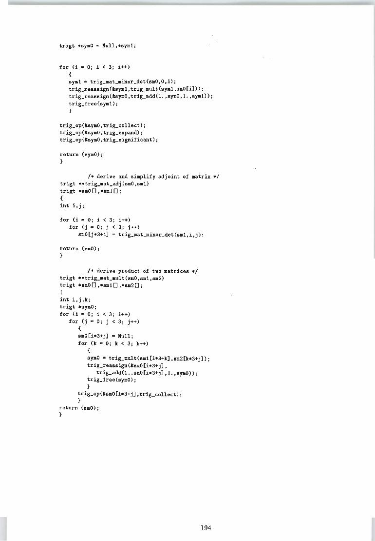
trigt .symO - Hull,.sym1;
for (i - 0; i < 3; i++) {
sym1 - trig_mat_minor_det(smO,O,i); trig_reassign(lsym1,trig_mult(sym1,smO[i)); trig_reassign(lsymO,trig_add(1.,symO,1.,sym1» ; trig_free(sym1); }
trig_op(lsymO,trig_collect); trig_op(lsymO,trig_expand); trig_op(lsymO,trig_significant);
return (symO); }
/. derive and simplify adjoint of matrix ./ trigt •• trig_mat_adj(smO,sm1) trigt .smO [) ,.sm1 0 ; {
int i,j;
for (i • 0; i < 3; i++) for (j - 0; j < 3; j++)
smO[j.3+i) - trig_mat_minor_det(sm1 ,i ,j) ;
return (smO); }
/. derive product of tvo matrices ./ trigt •• trig_mat_mult(smO,sm1,sm2) trigt .smO [) , .sm1 0 , .sm2 0 ; {
int i,j,k; trigt .symO; for (i - 0; i < 3; i++)
for (j - 0; j < 3; j++) {
smO[i.3+j) - Hull; for (k • 0; k < 3; k++)
{
symO - trig_mult(sml[i.3+k),sm2[k.3+j); trig_reassign(lsmO[i.3+j),
trig_add(1.,smO[i.3+j),l . ,symO»; trig_free(symO); }
trig_op(lsmO[i.3+j),trig_collect) ; }
return (smO); }
194
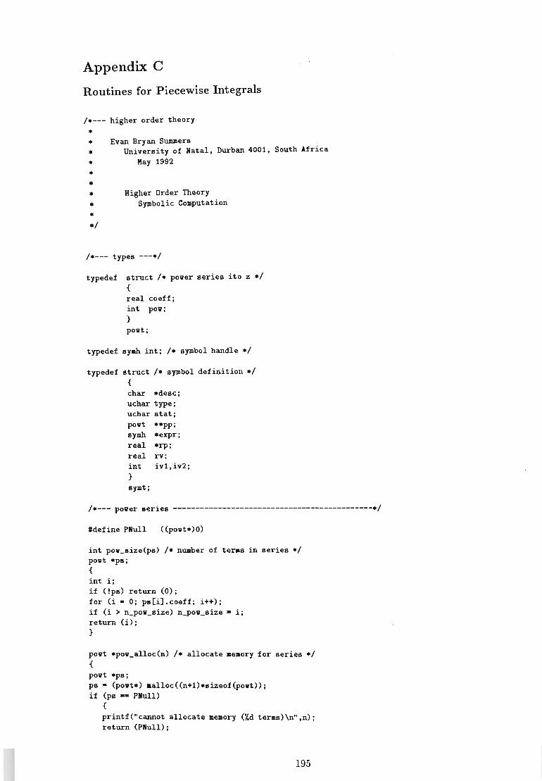
Appendix C
Routines for Piecewise Integrals
/*--- higher order theory
* * Evan Bryan Summers * University of Hatal, Durban 4001, South Africa * Kay 1992
* * * Higher Order Theory * Symbolic Computation
* */
typedef struct /* power series ito z */ {
real coeff: int pow: }
powt:
typedef symh int: /* symbol handle */
typedef struct /* symbol definition */ {
char *desc: uchar type: uchar stat: powt **pp: s}'llh *expr: real *rp: real rv: int iv1,iv2: }
s}'1lt;
/*--- power series ---------------------------------------------*/
Idef ine PHull «powU)0)
int pow_size(ps) /* nuaber of teras in series */ powt *ps: {
int i: if (!ps) return (0): for (i - 0: ps[i).coeff: i++): if (i > n_pow_size) n_pow_size • i: return (i): }
powt *pow_alloc(n) /* allocate aeaory for series */ {
powt *ps: ps - (powt*) aalloc«n+1)*sizeof(povt»: if (ps _. PHull)
{
printf("cannot allocate aemory (%d teras)\n",n): return (PHull) j
195
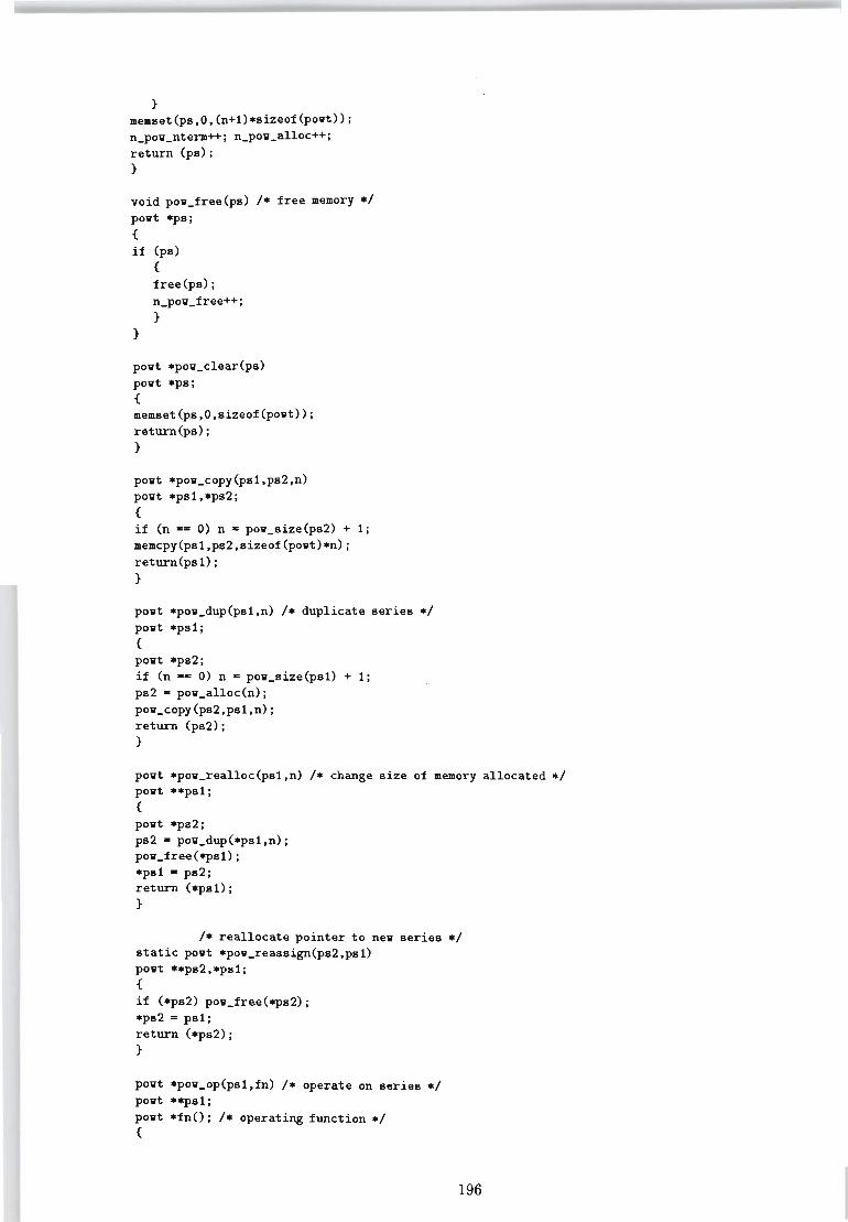
}
memset(ps,O,(n+l)*sizeof(povt»; n_pov_nterm++; n_pov_alloc++; return (ps); }
void pov_free(ps) /* free memory */ povt *ps; {
if (ps)
}
{
free(ps); n_pov_free++; }
povt *pov_clear(ps) povt *ps; {
memset(ps,O,sizeof(povt»; return(ps) ; }
povt *pov_copy(psl,ps2,n) povt *psl,*ps2; {
if (n z= 0) n • pov_size(ps2) + 1; memcpy(psl,ps2,sizeof(povt)*n); return(ps1} ; }
povt *pov_dup(psl,n) /* duplicate series */ povt *psl; {
povt *ps2; if (n -- 0) n - pov_size(psl) + 1; ps2 - pov_alloc(n); pov_copy(ps2,psl,n); return (ps2); }
povt *pov_realloc(psl,n) /. change size of memory allocated */ povt •• psl; {
povt *ps2; ps2 - pov_dup(*psl,n); pov _free ( *psi) ; *psl - ps2; return (.psl); }
/. reallocate pointer to nev series ./ static povt .pov_reassign(ps2,psl) povt •• ps2,*ps1; {
if (.ps2) pov_free(*ps2); .ps2 -= psl; return (.ps2); }
povt .pov_op(psl,fn) /. operate on series ./ povt •• psl; povt .fn(); /. operating function */ {
196
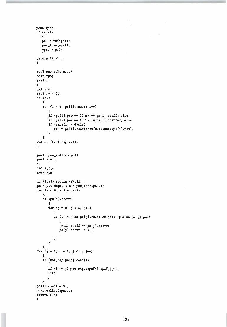
povt .ps2; if (.psl)
{
ps2· fn(.psl); pov_free(.ps1) ; .psl • ps2; }
return (.psl); }
real pov_calc(ps,z) povt .ps; real z; {
int i,n; real rv = 0.; if (ps)
{
for (i • 0; ps[i] . coeff; i++) {
if (ps[i].pov == 0) rv += ps[i] .coeff; else if (ps[i].pov -= 1) rv +- ps[i].coeff*z; else if (fabs(z) > dvsig)
rv +- ps[i] . coeff*pov(z,(double)ps[i] . pov); }
}
return (real_sig(rv»; }
povt *pov_collect(psl) povt *psl; {
int i,j,n; povt *ps;
if (!psl) return (PHull); ps • pov_dup(psl,n - pov_size(psl»; for (i • 0; i < n; i++)
{
if (ps[i].coeff) {
for (j .. 0; j < n; j++) {
if (i !- j tt ps[j].coeff 1t ps[i ] .pov -= ps[j].pov) {
}
}
}
ps[i].coeff += ps[j] . coeff; ps[j].coeff - 0.; }
for (j • 0, i • 0; j < n; j++) {
if (chk_sig(ps[j].coeff» {
if (i !- j) pov_copy(lps[i],lps[j],l) ; i++; }
}
ps[i].coeff·O.; pov_realloc(lps,i); return (ps); }
197
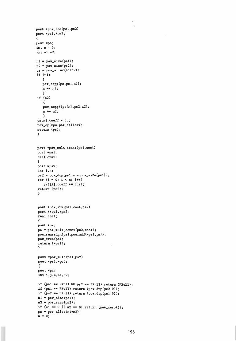
povt *pov_add(psl,ps2) povt *psl,*ps2; {
povt *ps; int n - 0; int nl,n2;
nl - pov_size(psl); n2 - pov_size(ps2); ps - pov_alloc(nl+n2); if (nO
{
pov_copy(ps,psl,nl); n +- nl; }
if (n2) {
pov_copy(tps[n),ps2,n2); n +- n2; }
ps[n).coeff - 0.; pov_op(tps,pov_collect); return (ps); }
povt *pov_mult_const(psl,cnst) povt *psl; real cnst; {
povt *ps2; int i,n; ps2 - pov_dup(psl,n - pov_size(psl»; for (i - 0; i < n; i++)
ps2[i).coeff *- cnst; return (ps2); }
povt *pov_sua(psl,cnst,ps2) povt **psl,*ps2; real cnst; {
povt *ps; ps - pov_ault_const(ps2,cnst); pov_reassign(psl,pov_add(*psl,ps»; pov_free(ps) ; return (*psO; }
povt *pov_ault(psl,ps2) povt *psl,*ps2; {
povt *ps; int i,j,n,nl,n2;
if (psl -- Plull tt ps2 -= Plull) return (Plull); if (psl -- Plull) return (pov_dup(ps2,O»; if (ps2 -- Plull) return (pov_dup(psl,O»; nl - pov_size(psl); n2 - pov_size(ps2)j if (nl .. 0 I I n2 -- 0) return (pov_zero(»j ps - pov_alloc(nl*n2); n - OJ
198
for (i - 0; i < nl; i++) for (j • 0; j < n2; j++)
{
ps[n].coeff - psl[i].coeff*ps2[j].coeff; ps[n].pov - psl[i].pov+ps2[j].pov; n++; }
ps[n].coeff·O.; pov_op(lps,pov_collect); return (ps); }
povt *pov_integrate(psl,zO,cnst) povt *psl; real zO,cnst; {
int i,j ,n; povt *ps; if (!psl) return (PNull); n - pov_size(psl); ps - pov_dup(psl,n + 1); for (i - 0; i < n; i++)
{
ps[i].pov++; ps[i].coeff /- (real) ps[i].pov; }
ps[n].coeff - - pov_calc(ps,zO) + cnst; ps[n].pov - 0; n++; ps[n].coeff - 0; return (ps); }
povt *pov_define(args) char args; {
povt *ps; int n - 0, ns - 8; char *arg; ps • pov_alloc(ns); for (arg - largs; *(real*)arg;)
{
ps[n].coeff. * (double*)arg; arg +- sizeof(double); ps[n].pov. *(int*)arg; arg +- sizeof(int); n++; }
ps[n].coeff - 0.; pov_realloc(lps,n); return (ps); }
/.--- syabolic expressions -----------------------______________ */
static int sya_size(se) /. nuaber of teras in series ./ syah .se; {
int n; if (!se) return (0); for (n - 0; se[n]; n++); return (n); }
static syah .sya_alloc(n) /. allocate .e.ory for series ./ {
199
syah *se: se • (syah*) .alloc«n+l)*sizeof(symh»: if (se ... Hull)
{ printf(ltcannot allocate .emory (%d terms)\nlt,n): return (Hull): }
n_sYJD_nsYJD++ : n_sYJD_alloc++: .emset(se,O,(n+l)*sizeof(symh»: return (se): }
static void sYJD_free(se) 1* free .e.ory *1 syah *se: {
if (se)
}
{
free(se): n_sYJD_free++: }
static syah *sYJD_copy(sel,se2,n) syah *sel,*se2: {
if (n .s 0) n • sYJD_size(se2) + 1: .emcpy(sel,se2,sizeof(symh)*n): return(sel): }
static syah *sya_dup(sel,n) 1* duplicate series *1 s)'llh *sel: {
syah *se2: if (n •• 0) n • sYJD_size(sel): se2 • sYJD_alloc(n): sya_copy(se2,sel,n): se2[n] = 0: return (se2); }
1* Change size of .emory allocated *1 static syah *sya_realloc(sel,n) syah **sel; {
s)'llh *se2; se2 • sya_dup(*sel,n): sYJD_free(*se1) : *sel • se2: return (*se1): }
1* reallocate pointer to new series *1 static s)'llh *sYJD_reassign(se2,sel) syah **se2,*sel; {
if (*se2) sya_free(*se2); *se2 • sel; return (*se2): }
static syah sya_define(desc,is,type) char *desc:
200
syah is; int type; {
int i; char *arg;
arg· (char*)ltype + sizeof(int);
sym[is].desc - desc; sym[is].type - type;
if (sym[is].type·- SymConst) {
sym[is].rv - *(real*)arg ; arg +- sizeof(double); }
else if (sym[is].type .- SymMConst)
{
sym[is].rp· *(real**)arg; arg +- sizeof(void*); }
else if (sya[is].type·- SymZ)
{
sym[is] . ivl - *(int*)arg; arg += sizeof(int) ; }
else if (sym[is].type .- SymExpr)
{
sym[is].expr· sym_dup«syah*)arg.O) ; }
else if (sya[is].type _. Syalnt)
{
sya[is].ivl - *(int*)arg; arg +- sizeof(int); sya[is].expr· sym_dup«symh*)arg.O) ; }
else if (sya[is].type .- SymLamlnt)
{
sya[is].ivl • *(int*)arg; arg +. sizeof(int) ; sya[is].iv2 • *(int*)arg; arg +- sizeof(int); sya[is].expr - sya_dup«syah*)arg.O) ; }
else {
fprintf(fdeb."error: sym: define\n") ;
return (0); }
sya_output(flog.is);
return (is); }
static syah *sya_tera(se) syah *se; {
int i; if (!se) return (Null); for (i - 0; se[i] II se[i] !- SymPlus; i++); if (!i) return (Null); return (sya_dup(se.i» ; }
201
static syah *sya_tail(se) syah *se; {
int i; if (se)
{ for (i = 0; se[i] tt se[i] != SymPlus; i++);
if (se[i] -= SymPlus) return (sya_dup(se+i+1,0»;
}
return (Hull); }
static int sya_term_si ze(se) syah *se; {
int i; if (!se) return (0); for (i - 0; se[i] tt se[i] !- SymPlus; i++); return (i); }
static int sym_tail_si ze(se) symh *se; {
int i; if (se)
{
for (i - 0; se[i] tt se[i] !- SyaPlus; i++); if (se[i] -- SyaPlus)
return (sya_size(se+i+1»; }
return (0); }
povt *sya_expand(k,is , se) syah is; s)'llh se [] ; {
povt *ret - Hull;
if (k < 1) { n_err++; return (Hull);}
if (is -- SyaHone) ret - lull; else if (is -- SyaExpr tt (!se I I !se[O]» ret - lull; else if (is -- SyaExpr)
{
syah *spO,*sp1; povt *ps;
spO - sya_tera(se+1); sp1 - sya_tail(se+1);
ret - sya_expand(k,se[O]);
if (spO) {
ps - sya_expand(k,SymExpr,spO); pov_reassign(lret,pov_ault(ret,ps»; pov_free(ps); sya_free(spO);
202
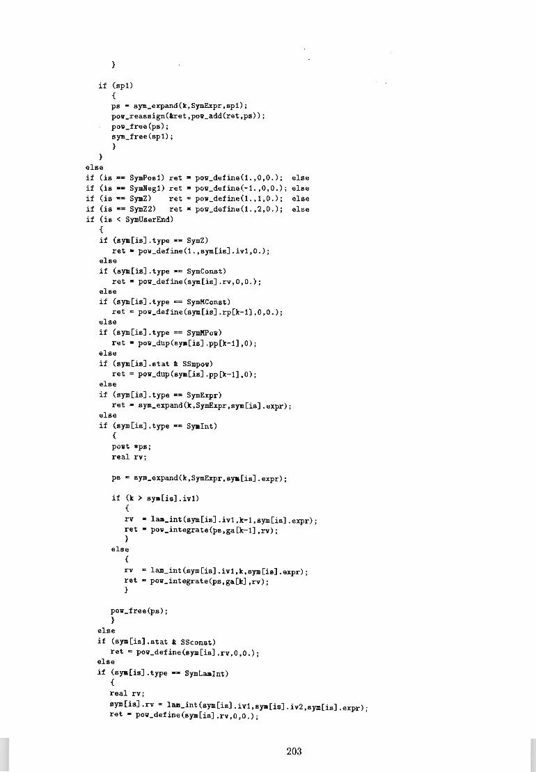
}
if (spi) {
} else
ps - sym_expand(k,SymExpr,spi); pov_reassign(lret,pov_add(ret,ps»; pov_free(ps); sym_free(spi); }
if (is -- SymPosi) ret - pov_define(l.,O,O.); else if (is -- SymMegi) ret - pov_define(-l.,O,O.); ~lse if (is -- SymZ) ret = pov_define(l.,l,O . ); else if (is -- SymZ2) ret = pow_define(1.,2,O.); else if (is < SymUserEnd)
{ if (sym[is].type -- SymZ)
ret - pow_define(l.,sym[is].ivi,O.); else if (sym[is].type -- SymConst)
ret - pow_define(sym[is].rv,O,O.); else if (sym[is].type -- SymMConst)
ret - pow_define(sym[is].rp[k-i],O,O.); else if (sym[is].type -= SymMPow)
ret • pow_dup(sym[is].pp[k-i],O); else if (sym[is].stat 1 SSmpov)
ret - pov_dup(sym[is].pp[k-i]~O);
else if (sym[is].type -= SymExpr)
ret - sym_expand(k,SymExpr,sym[is].expr); else if (sym[is].type -- Symlnt)
{ powt .ps; real rv;
ps - sym_expand(k,SymExpr,sym[is].expr);
if (k> sym[is].ivi) { rv - lam_int(sya[is].ivi,k-i,sym[is].expr); ret - pov_integrate(ps,ga[k-i],rv); }
else { rv - lam_int(sym[is].ivi,k,sym[is].expr); ret - pow_integrate(ps,ga[k],rv); }
pow_free(ps); }
else if (sym[is].stat 1 SSconst)
ret • pov_define(sym[is].rv,O,O.); else if (sym[is].type -- SymLamlnt)
{ real rv;
sym[is].rv - lam_int(sym[is].ivl,sya[is].iv2,sym[is].expr); ret - pow_define(sym[is].rv,O,O.);
203
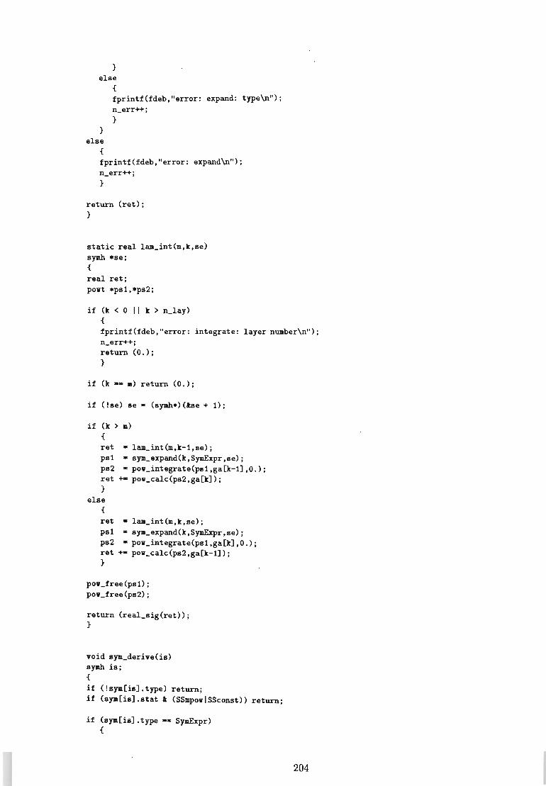
}
else
}
{
fprintf(fdeb,"error: expand: type\n" ) ; n_err++; }
else {
fprintf(fdeb,"error: expand\n"); n_err++; }
return (ret); }
static real lam_int(m,k,se) symh .se; {
real ret; povt .psl,.ps2;
if (k < 0 II k > n_lay) {
fprintf(fdeb,"error: integrate: layer number\n") ; n_err++; return (0.); }
if (k --.) return (0.);
if (!se) se - (symh.) (lse + 1);
if (k > m) {
ret - lam_int(m,k-l,se); psl - sym_expand(k,SymExpr,se); ps2 - pov_integrate(psl,ga[k-l] ,0.) ; ret +- pov_calc(ps2,ga[k]); }
else {
ret - lam_int(m,k,se): psl - sym_expand(k,SyaExpr,se); ps2 - pov_integrate(psl,ga[k] ,0.); ret +- pov_calc(ps2,ga[k-l]); }
pov_free(psl) ; pov_free(ps2);
return (real_sig(ret» ; }
void sya_derive(is) symh is; {
if (!sya[is].type) return; if (sya[is].stat l (SSmpovISSconst» return ;
if (sya[is].type -- SyaExpr) {
204

int i, n; sym[is].pp. (powt **) aalloc(n s n_lay*sizeof(powt*»; aemset«void*)sym[is].pp,O,n); for (i - 0; i < n_lay; i++)
sym[is].pp[i] - sym_expand(i+1,SymExpr,sya[is].expr); sya[is].stat I- SSmpow; }
else if (sym[is].type -- Symlnt)
{ powt *ps; real rv; int i, n, at
sym[is].pp - (powt **) malloc(n E n_lay*sizeof(powt*»; aeaset«void*)sym[is].pp,O,n); rv - 0.; for (m - sym[is].iv1; m > 0; a--)
{ ps - sya_expand(a,SymExpr,sya[is].expr); sya[is].pp[a-1] - pov_integrate(ps,ga[a],rv); rv - pow_calc(sya[is].pp[a-1],ga[a-1]); pow_free(ps); }
rv·O.; for (m - sym[is].iv1 + 1; m <- n_lay; m++)
{ ps s sym_expand(m,SymExpr,sym[is].expr); sym[is].pp[m-1] • pow_integrate(ps,ga[a-1],rv); rv· pow_calc(sym[is].pp[a-1],ga[a]); pow_free(ps); }
sya[is].stat 1- SSapow; }
else if (sym[is].type _. SymLamlnt)
{ sya[is].rv.lam_int(sym[is].iv1,sym[is].iv2,sym[is].expr); sym[is].stat I- SSconst; }
}
real sym_eval(is,k,z) syah is; real z; { real ret;
if (sym[is].type .- SymZ) return (pov(z,l.*sym[is].iv1»;
else if (sym[is].type -- SymConst)
return (sym[is].rv);
if (sya[is].stat 1 SSconst) return (sya[is].rv);
else if (sya[is].type.- SymLamlnt)
return (laa_int(sym[is].iv1,sya[is].iv2,sya[is].expr»;
if (sya[is].type •• SyaMConst) return (sym[is].rp[k-1]);
205
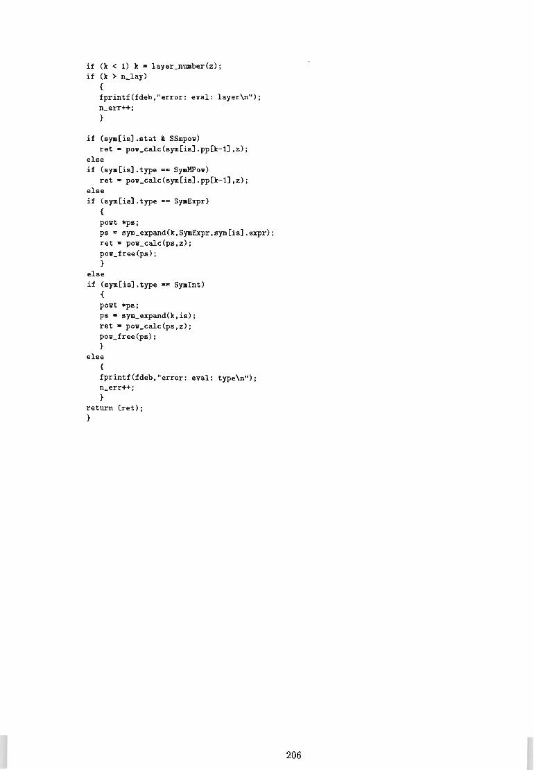
if (k < 1) k - 1ayer_number(z); if (k > n_1ay)
{ fprintf(fdeb,"error: eva1: 1ayer\n"); n_err++; }
if (sym[is].stat t SSmpov) ret. pov_calc(sym[is].pp[k-1],z);
else if (sym[is].type _. SymMPov)
ret. pov_calc(sym[is].pp[k-1],z); else if (sym[is].type .- SymExpr)
{
povt .ps; ps - sym_expand(k,SymExpr,sym[is].expr); ret - pov_calc(ps,z); pov_free(ps); }
else if (sym[is].type·- Symlnt)
{
povt .ps; ps - sym_expand(k,is); ret - pov_calc(ps,z); pov_free(ps) ; }
else {
fprintf(fdeb,"error: eva1: type\n"); n_err++; }
return (ret); }
206
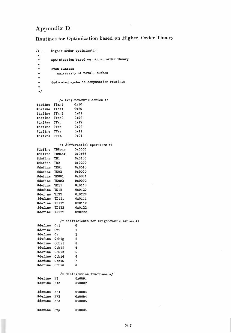
Appendix D
Routines for Optimization based on Higher-Order Theory
/.--- higher order optimization
• • optiaization based on higher order theory
• • evan sUDllllers • university of natal, durban
• • dedicated symbolic computation routines
• ./
/. trigonometric series ./ 'define TTsnl Oxl0 'define TTcsl Ox20 'define TTsn2 OxOl #define TTcs2 Ox02 #define TTsc Ox12 #define TTcc Ox22 #define TTss Oxll #define TTcs Ox21
/. differential operators ./ #define TON one OxOOOO #define TOKask OxOfff 'define TOl OxOl00 #define T02 Ox0200 #define TOOl Ox0010 #define T002 #define TOOOl #define T0002 #define TOl1 #define T012 #define T022 #define T0111 #define T0112 'define T0122 #define TD222
Ox0020 OxOOOl Ox0002 Ox0110 Ox0120 Ox0220 Ox0111 Ox0112 Ox0122 Ox0222
/. coefficients for trigonometic series ./ #define Cul 0 #define Cu2 1 #define Cv 2 'define Cchig 2 #define Cchil 3 'define Cchi2 4 #define Cchi3 5 'define Cchi4 6 'define Cchi5 7 'define Cchi6 8
/. distribution functions ./ #define Ff OxOOOl 'define Ffs Ox0002
'define FFl Ox0003 #define FF2 Ox0004 'define FF3 Ox0005
#define Ffg Ox0005
207
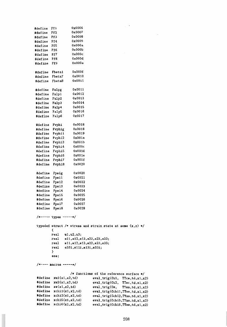
'define Ff1 OxOO06 'define Ff2 OxOO07 'define Ff3 OxOO08 'define Ff4 OxOO09 'define Ff5 OxOOOa 'define Ff6 OxOOOb 'define Ff7 OxOOOc 'define Ff8 OxOOOd 'define Ff9 OxOOOe
'define Fbeta1 OxOOOf 'define Fbeta7 Ox0010 'define Fbeta8 OxOO11
'define Falpg OxOO11 'define Falp1 OxOO12 'define Falp2 OxOO13 'define Falp3 OxOO14 'define Falp4 OxOO15 'define Falp5 OxOO16 'define Falp6 OxOO17
'define Fvphi OxOO18 'define Fvphig OxOO18 'define Fvphit OxOO19 'define Fvphi2 Ox001a 'define Fvphi3 Ox001b 'define Fvphi4 Ox001c 'define Fvphi5 Ox001d 'define Fvphi6 Ox001e 'define Fvphi7 Ox001f 'define Fvphi8 Ox0020
'define Fpsig Ox0020 'define Fpsit Ox0021 'define Fpsi2 Ox0022 'define Fpsi3 Ox0023 'define Fpsi4 Ox0024 'define Fpsi5 Ox0025 'define Fpsi6 Ox0026 'define Fpsi7 Ox0027 'define Fpsi8 Ox0028
/*----- types -----*/
typedef struct /* stress and strain state at so.e (x,z) */ {
real u1,u2,u3; real e11,e12,e13,e22,e23,e33; real sll,s12,813,s22,823,s33; real e33i,slli,813i,s33i; }
sss;
/*---- macros -----*/
/* functions of the reference surface */ 'define xu1(x1,x2,td) eval_trig(Cu1, TTcs,td,x1,x2) 'define xu2(x1,x2,td) eVal_trig(Cu2, TTsc,td,x1,x2) 'define xv(x1,x2,td) eval_trig(Cv, TTss,td,xl,x2) 'define xchil(x1,x2,td) eval_trig(Cchi1,TTss,td,x1,x2) 'define xchi2(x1,x2,td) eval_trig(Cchi2,TTss,td,x1,x2) 'define xchi5(x1,x2,td) eval_trig(Cchi5,TTss,td,x1,x2) 'define xchi6(x1,x2,td) eval_trig(Cchi6,TTss,td,x1,x2)
208

'define xchi(icf ,xl,x2, td) eval_trig(Cchig+icf, TIss, td,xl,x2)
/*---- globals -----*/
/* geometry */ int n_lay, a_ref; real gh,ga[Mn+l],gbl,gb2; real gkll,gk12,gk22,gk21;
/* aaterial properties */ real ael[Mn],ae2[Mn],agl[Mn],ag2[Mn]; real anul [Mn] ,anu2[Mn) ; real meO [Mn] ,anuO [Mn] ; real aall[Mn],aa12[Mn),ma13[Mn],ma33[Mn);
/* coefficients of distribution functions */ real cfd[41] [Mn] [Mp+l] ;
/*----- material -----*/
void aat_depend(void) /* calculate dependent aaterial constants */ {
int i; real mdel,adelll,adel12,adel13,adel33;
for (i s 0; i < n_lay; i++) {
- ael [i] / (1 - anu1[i] *anul [i]) ; aeO[i] anuO[i] - ael[i]/me2[i]*mnu2[i]/(1 - anul[i]);
- (1 + mnu1[i]); adel adel adel adel11 ade1l2 ade1l2 ade1l3 adel33
*- (1 - anul[i] - 2*mnu2[i]*anu2[i]*ael[i]/me2[i]); /s (mel[i]*mel[i]*me2[i]); - (1 - anu2[i]*anu2[i] .. el[i]/ae2[i])/ael[i]/ae2[i]; • (anul[i] + anu2[i]*anu2[i]*ael[i]/ae2[i]);
/- ae1[i]/ae2[i]; - anu2[i]*(1 + anul[i])/ael[i]/ae2[i]; • (1 - anu1[i] *IIIIlu1[i] ) /ae1[i] /ae1[i] ;
}
aal1[i] aa12[i] aa13 [i] aa33[i] }
- ade1l1/adel; - ade1l2/adel; - ade1l3/adel; - adel33/mdel;
/*----- coaputation of coefficients -----*/
/* set coefficents to zero */ void coeff_clear(real cf[Mn] [Mp+l]) {
int i,k;
for (k - 1; k <- n_lay; k++) for (i - 0; i <- Mp; i++)
cf [k] [i] - 0;
return; }
/* add a tera to a series
209
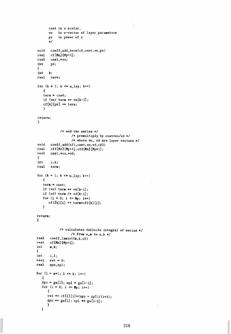
cnst is a scalar, vn is n-vector of layer paraaeters pz is power of z */
void coeff_add_term(cf,cnst,vn,pz) real cf[Mn][Hp+1]; real cnst,*vn; int pz; {
int k; real term;
for (k - 1; k <- n_lay; k++) {
term - cnst; if (vn) term *- vn[k-1]; cf[k] [pz] +"" term; }
return; }
/* add two series */ /* preaultiply by cnst*vn/vd */ /* where vn, vd are layer vectors */
void coeff_add(cf1,cnst,vn,vd,cf2) real cf 1 [Mn] [Mp+1] , cf2 [Mn] [Hp+1] ; real cnst,*vn,*vd; {
int i,k; real term;
for (k - 1; k <- n_lay; k++) {
tera - cnst; if (vn) tera *- vn[k-1]; if (vd) tera /- vd[k-1]; for (i - 0; i <- Hp; i++)
cf1[k] [i] +- tera*cf2[k] [i]; }
return; }
/* calculates definite integral of series */ /* froa a_a to a_k */
real coeff_laaint(a,k,cf) real cf [Mn] [Mp+1J ; int a,k; {
int i,l; real ret - 0; real zpu,zpl;
for (1 - a+1; 1 <- k; 1++) {
zpu - ga[l]; zpl - ga[l-lJ; for (i - 0; i <- Hp; i++)
}
{
ret +- cf[l] [i]*(zpu - zpl)/(i+1)j zpu *- ga[l]; zpl *. ga[l-l]j }
210

return (ret); }
/* evaluates a series */ real coeff_eval(cf,z) real dO; real z; {
int i; real zp - 1, ret - 0;
for (i - 0; i <- Mp; i++) , {
ret +- cf[i]*zp; zp *- z; }
return (ret); }
/* integrates a series fro. a_a to z */ real coeff_layint(cfO,m,cfn) real dO[Mn] [)tp+l] ,dn[Mn] [Mp+1]; int a; {
int i,l; real term; real zpu, zpl;
for (term - 0, 1 - a; 1 >- 1; 1--) {
dO[l] [0] - 0; for (i • 0; i < Mp; i++)
dO[l] [i+l] - cfn[l] [i]/(i+1); dO [1] [0] • tera - coeff_eval (dO [1] ,ga[l]); term· coeff_eval(cfO[l],ga[l-l]); }
for (term - 0, 1 - .+1; 1 <- n_lay; 1++) {
dO[l] [0] • 0; for (i - 0; i < Mp; i++)
cfO[l][i+l] - cfn[l] [i]/(i+l); cfO[l] [0] - tera - coeff_eval(cfO[l],ga[l-l]); tera - coeff_eval(cfO[l],ga[l]); }
return (tera); }
/*----- distribution functions -----*/
/* evaluates distribution function */ real zfn(int fn, int k, real z) {
int i; real ret - 0, zp - 1;
for (i - 0; i <- 6; i++) {
ret +- cfd[fn] [k][i]*zp; zp *- z; }
211
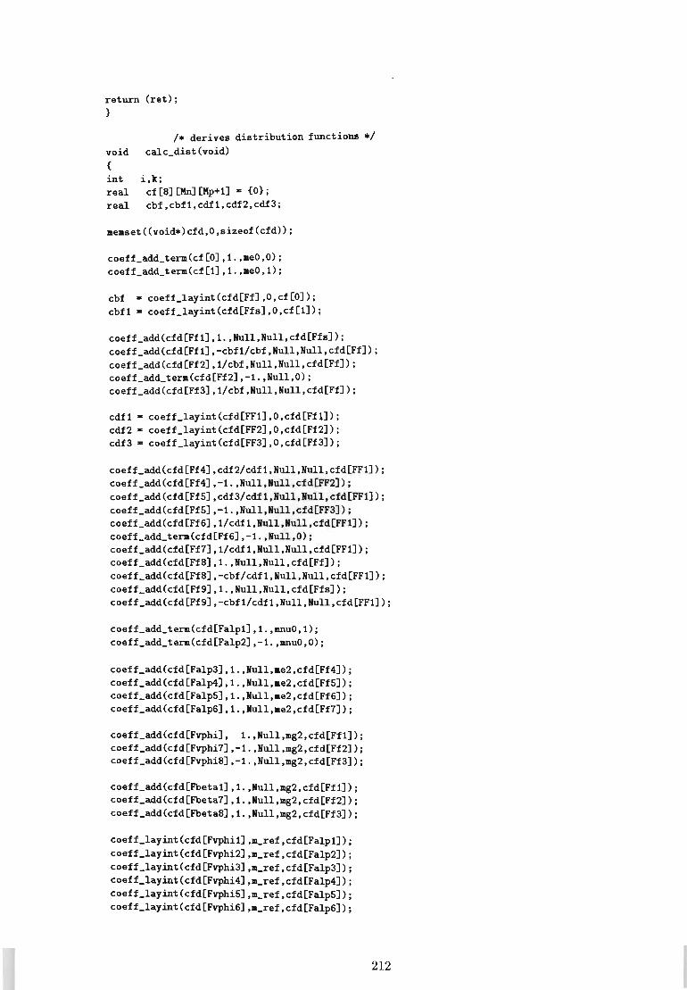
return (ret); }
/* derives distribution functions */ void calc_dist(void) {
int i,k; real cf[8] [Mn] [Mp+1] • {O}; real cbf,cbf1,cdf1,cdf2,cdf3;
memset«void*)cfd,O,sizeof(cfd»;
coeff_add_term(cf[O],1.,meO,O); coeff_add_term(cf[1],1.,meO,1);
cbf • coeff_layint(cfd[Ff],O,cf[O]); cbf1 • coeff_layint(cfd[Ffs],O,cf[1]);
coeff_add(cfd[Ff1],1.,Hull,Hull,cfd[Ffs]); coeff_add(cfd[Ffl],-cbfl/cbf,Hull,Hull,cfd[Ff]); coeff_add(cfd[Ff2],1/cbf,Hull,Hull,cfd[Ff]); coeff_add_term(cfd[Ff2],-1.,Hull,O); coeff_add(cfd[Ff3],1/cbf,Hull,Hull,cfd[Ff]);
cdfl • coeff_layint(cfd[FF1],O,cfd[Ffl]); cdf2 = coeff_layint(cfd[FF2],O,cfd[Ff2]); cdf3 • coeff_layint(cfd[FF3],O,cfd[Ff3]);
coeff_add(cfd[Ff4],cdf2/cdfl,Hull,Hull,cfd[FF1]); coeff_add(cfd[Ff4],-1.,Hull,Hull,cfd[FF2]); coeff_add(cfd[Ff5],cdf3/cdfl,Hull,Hull,cfd[FF1]); coeff_add(cfd[Ff5],-1.,Hull,Hull,cfd[FF3]); coeff_add(cfd[Ff6],1/cdfl,Hull,Hull,cfd[FF1]); coeff_add_term(cfd[Ff6],-1.,Hull,O); coeff_add(cfd[Ff7],l/cdfl,Hull,Hull,cfd[FF1]); coeff_add(cfd[Ff8],1.,Hull,Hull,cfd[Ff]); coeff_add(cfd[Ff8],-cbf/cdfl,Hull,Hull,cfd[FF1]); coeff_add(cfd[Ff9],l.,Hull,Hull,cfd[Ffs]); coeff_add(cfd[Ff9],-cbf1/cdfl,Hull,Hull,cfd[FF1]);
coeff_add_term(cfd[Falpl],l.,mnuO,l); coeff_add_term(cfd[Falp2],-1.,mnuO,O);
coeff_add(cfd[Falp3],1.,Hull,me2,cfd[Ff4]); coeff_add(cfd[Falp4],l.,Hull,me2,cfd[Ff5]); coeff_add(cfd[Falp5],l.,Hull,me2,cfd[Ff6]); coeff_add(cfd[Falp6],l.,Hull,me2,cfd[Ff7]);
coeff_add(cfd[Fvphi], 1.,Hull,mg2,cfd[Ff1]); coeff_add(cfd[Fvphi7],-1.,Hull,mg2,cfd[Ff2]); coeff_add(cfd[Fvphi8],-1.,Hull,mg2,cfd[Ff3]);
coeff_add(cfd[Fbetal],1.,Hull,mg2,cfd[Ffl]); coeff_add(cfd[Fbeta7],l.,Hull,mg2,cfd[Ff2]); coeff_add(cfd[Fbeta8],l.,Hull,mg2,cfd[Ff3]);
coeff_layint(cfd[Fvphi1],m_ref,cfd[Falpl]); coeff_layint(cfd[Fvphi2],m_ref,cfd[Falp2]); coeff_layint(cfd[Fvphi3],m_ref,cfd[Falp3]); coeff_layint(cfd[Fvphi4],m_ref,cfd[Falp4]); coeff_layint(cfd[Fvphi5],m_ref,cfd[Falp5]); coeff_layint(cfd[Fvphi6],m_ref,cfd[Falp6]);
212
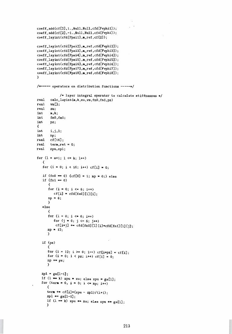
coeff_add(cf[2] ,1. ,Null ,Null ,cfd[Fvphi 1]); coeff_add(cf[2],-1.,Nu11,Nu11,cfd[Fvphi]); coeff_1ayint(cfd[Fpsi1],m_ref,cf[2]);
coeff_1ayint(cfd[Fpsi2],m_ref,cfd[Fvphi2]); coeff_1ayint(cfd[Fpsi3],m_ref,cfd[Fvphi3]); coeff_1ayint(cfd[Fpsi4], __ ref,cfd[Fvphi4]); coeff_1ayint(cfd[Fpsi5], __ ref,cfd[Fvphi5]); coeff_1ayint(cfd[Fpsi6],a_ref,cfd[Fvphi6]); coeff_1ayint(cfd[Fpsi7], __ ref,cfd[Fvphi7]); coeff_1ayint(cfd[Fpsi8],m_ref,cfd[Fvphi8]); }
/*----- operators on distribution functions -----*/
/* layer integral operator to calculate stiffnesses */ real ca1c_1ayint(m,k,zu,vm,fnO,fn1,pz) real nO; real zu; int _,k; int fnO,fn1; int pz; {
int i,j,l; int np; real cf[16] ; real term,ret = 0; real zpu, zp1;
for (1 - m+1; 1 <= k; 1++) {
for (i - 0; i < 16; i++) cf[i] - 0;
if (fnO -- 0) {cf[O] - 1; np - O;} else if (fn1 -- 0)
{
for (i - 0; i <- 6; i++) cf [i] - cfd[fnO] [1] [i] ;
np - 6; }
else {
for (i - 0; i <= 6; i++) for (j - 0; j <- 6; j++) cf[i+j] +- cfd[fnO] [1] [i]*cfd[fn1] [1] [j];
np - 12; }
if (pz) {
for (i - 12; i >- 0; i--) cf[i+pz] - cf[i]; for (i - 0; i < pz; i++) cf[i] - 0; np += pz; }
zp1 - ga[1-1]; if (1 -- k) zpu - zu; else zpu - ga[l]; for (term - 0, i - 0; i <= np; i++)
{
term +- cf[i]*(zpu - zp1)/(i+1); zp1 *- ga[1-1]; if (1 -- k) zpu *- zu; else zpu *- ga[l]. } ,
213
if (va) tera.- vm[l-l);
ret +- term; }
return (ret); }
real real
/. definite layer integral fro. a_O to a_n ./ calc_laaint(vm,fnO,fn1,pz) vaO;
{
int real real real
i,j,np,k; cf [16) ; tera,ret - 0; zpu,zpl;
for (k - 1; k <- n_lay; k++) {
for (i - 0; i < 16; i++) cf[i) - 0;
if (fnO -- 0) {cf[O) - 1; np - O;} else if (fn1 -- 0)
{
for (i - 0; i <- 6; i++) cf [i) - cfd[fnO) [k) [i) ;
np - 6; }
else {
for (i - 0; i <- 6; i++) for (j - 0; j <- 6; j++) cf[i+j) +- cfd[fnO) [k) [i).cfd[fn1) [k) [j);
np - 12; }
if (pz) {
for (i - 12; i >- 0; i--) cf[i+pz) - cf[i); for (i - 0; i < pz; i++) cf[i) - 0; np +- pz; }
zpu - ga[k); zpl - ga[k-1); for (term - 0, i - 0; i <= np; i++)
{
tera +- cf[i).(zpu - zpl)/(i+1); zpu.- ga[k]; zpl .- ga[k-1]; }
if (va) tera.- va[k-1);
ret +- tera; }
return (ret); }
/.----- integrated stiffnesses -----./
'define cbg(g) 'define cbgb(g) 'define ccg(g) 'define ccgb(g) 'define ccOg(g)
calc_laaint(.a11,Fpsig+g,O,O) calc_laaint(.a12,Fpsig+g,O,O) calc_laaint(.a11,Fvphig+g,O,O) calc_laaint(.a12, Fvphig+g,O, 0) calc_laaint(.a11,Fvphig+g,O,l)
214

#define cCOgb(g) ·calc_lamint(aa12, Fvphig+g, 0', 1) #define ccgq(g,q) calc_lamint (aall,Fpsig+g, Fvphig+q,O) 'define ccgqb(g,q) calc_lamint (aa12,Fpsig+g, Fvphig+q,O) #define cdOg(g) calc_lamint(mall,Fpsig+g,O,l) 'define cdOgb(g) calc_lamint(ma12,Fpsig+g,0,1) #define cdgq(g,q) calc_lamint(mall,Fpsig+g,Fpsig+q,O) #define cdgqb(g,q) calc_lamint(aa12,Fpsig+g,Fpsig+q,0) #define chg(g) calc_lamint(aa13,Falpg+g,0,0) #define chOg(g) calc_lamint(aa13,Falpg+g,0,1) #define chgq(g,q) calc_lamint(aa13,Fpsig+g,Falpg+q,0) #define clgq(g,q) calc_lamint(aal1,Fvphig+g,Fvphig+q,0) #define clgqb(g,q) calc_lamint(aa12,Fvphig+g,Fvphig+q,0) #define cpgq(g,q) calc_lamint(aa13,Fvphig+g,Falpg+q,0) #define cpgqb(g,q) calc_lamint(aa13,Falpg+g,Fpsig+q,0) #define crgq(g,q) calc_lamint (aa33, Falpg+g, Fvphig+q, 0) #define crgqb(g,q) calc_lamint(ma33,Falpg+g,Falpg+q,0) #define ctgq(g,q) calc_lamint(aall,Fvphig+g,Fpsig+q,O) #define ctgqb(g,q) calc_lamint (aa12, Fvphig+g, Fpsig+q, 0)
1* calculates integrated stiffnesses *1 void calc_stiff() {
cb - calc_lamint(aall,O,O,O); cbb - calc_lamint(aa12,0,0,0); cbO - calc_lamint(mall,O,O,l); cbOb - calc_lamint(ma12,0,0,1); cdOO - calc_lamint(mall,0,0,2); cdOOb - calc_lamint(ma12,0,0,2); cdl - calc_lamint(Hull,Ffl,Fbetal,O);
cbl - cbg(l); cblb - cbgb(l); cb2 - cbg(2); cb2b - cbgb(2); cb3 - cbg(3); cb3b - cbgb(3); cb4 - cbg(4); cb4b - cbgb(4); cbS - cbg(S); cbSb - cbgb(S); cb6 - cbg(6); cb6b - cbgb(6);
chl - chg(l); chOl - chOg(l); cdOl - cdOg(l); ch2 - chg(2); ch02 - chOg(2); cd02 - cdOg(2); ch3 - chg(3); ch03 - chOg(3); cd03 - cdOg(3); ch4 - chg(4); ch04 - chOg(4); cd04 - cdOg(4); chS - chg(S); ch05 - chOg(5); cd05 - cdOg(5); ch6 - chg(6); ch06 ~ chOg(6); cd06 - cdOg(6);
ccl - ccg(l); cclb - ccgb(l); ccOl - ccOg(l); ccOlb - ccOgb(l); cc2 - ccg(2); cc2b - ccgb(2); cc02 - ccOg(2); cc02b - ccOgb(2); cc3 - ccg(3); cc3b - ccgb(3); cc03 - ccOg(3); cc03b - ccOgb(3); cc4 - ccg(4); cc4b - ccgb(4); cc04 - ccOg(4); cc04b - ccOgb(4); cc5 • ccg(S); ccSb - ccgb(5); cc05 - ccOg(5); cc05b - ccOgb(S); cc6 - ccg(6); cc6b· ccgb(6); cc06. ccOg(6); cc06b - ccOgb(6);
ccll - ccgq(l,l); ccl1b. ccgqb(l,l); cc12 - ccgq(1,2)-; cc12b. ccgqb(1,2); cc21 • ccgq(2,1); cc21b • ccgqb(2,1); cc22 - ccgq(2,2); cc22b - ccgqb(2,2); cclS - ccgq(l,S); cclSb - ccgqb(l,S); cc16· ccgq(1,6); cc16b - ccgqb(1,6); cc2S - ccgq(2,S); cc25b. ccgqb(2,S); cc26 - ccgq(2,6); cc26b - ccgqb(2,6);
chll· chgq(l,l); cdll - cdgq(l,l); ch12 - chgq(l,2); cd12 - cdgq(1,2); ch2l - chgq(2,l); ch22 • chgq(2,2); cd22 - cdgq(2,2);
215
ch15 - chgq(1.5); cd15 - cdgq(1.5); ch16 • chgq(1.6); cd16 • cdgq(1.6); ch25 - chgq(2.5); cd25 - cdgq(2.5); ch26 - chgq(2.6); cd26 = cdgq(2.6);
cl11 • clgq(1.1); cl11b • clgqb(1.1): c112· clgq(1.2); c112b· clgqb(1.2); c121 • clgq(2.1); c121b • clgqb(2.1); c122· clgq(2.2); c122b - clgqb(2.2); c115 • clgq(1.5); c115b· clgqb(1.5); c116 • clgq(1.6); c116b· clgqb(1.6); c125· clgq(2.5); c125b - clgqb(2.5); c126· clgq(2.6); c126b - clgqb(2.6):
cp11 • cpgq(1.1); cp11b • cpgqb(1.1); cp12· cpgq(1.2); cp12b· cpgqb(1.2); cp21 • cpgq(2.1); cp21b· cpgqb(2.1): cp22 • cpgq(2.2); cp22b· cpgqb(2.2); cp15. cpgq(1.5); cp15b z cpgqb(1.5); cp16· cpgq(1.6); cp16b - cpgqb(1.6); cp25· cpgq(2.5); cp25b· cpgqb(2.5): cp26· cpgq(2.6): cp26b - cpgqb(2.6):
cr11 - crgq(1.1); cr11b - crgqb(1.1): cr12 • crgq(1.2); cr12b· crgqb(1.2): cr21· crgq(2.1); cr22· crgq(2.2); cr22b - crgqb(2.2); cr15· crgq(1.5); cr15b • crgqb(1.5); cr16 • crgq(1.6); cr16b. crgqb(1.6); cr25 • crgq(2.5); cr25b· crgqb(2.5); cr26· crgq(2.6); cr26b - crgqb(2.6);
ct11 • clgq(1.1); cl11b· ctgqb(1.1); ct12· clgq(1.2); c112b - ctgqb(1.2); ct21· clgq(2.1); c121b· ctgqb(2.1); ct22· clgq(2.2); c122b - ctgqb(2.2); ct15 • clgq(1.5); c115b. ctgqb(1.5); ct16 • clgq(1.6); c116b. ctgqb(1.6); ct25 - clgq(2.5): c125b - ctgqb(2.5); ct26 • clgq(2.6); c126b· ctgqb(2.6); }
/*----- governing equations -----*/
/* system of equations for plate */ void ays_plate(tc.qc .... vn.q3p.q3m) real tc[5] [5] .qc[5]; int ... wn; real q3p.q3m; {
real laa.laa_2.1aa_3.1aa_4; real gaa.gu_2.gu_3.gaa_4:
laa • va*M_PI/gb1; gaa • wn*M_PI/gb2;
10_2 • laa*laa; lu_3 - laa_2*laa; laa_4 - laa_3*laa; gu_2 • gam*gaa: gam_3 - gam_2*gam; gaa_4 • gaa_3*gam;
tc[O] [0] • -(cb*gaa_2)/2 + (cbb*gam_2)/2 - cb*laa_2; tc[O] [1] • -(cb*gam*lam)/2 - (cbb*gaa*laa)/2; tc[0][2] • cbO*gam_2*laa + cbO*laa_3; tc[O] [3] - ch1*laa + cb1*gam_2*laa + cb1*laa_3; tc[O] [4] • ch2*laa + cb2*gaa_2*laa + cb2*laa_3:
216
tc[l] [0] • -(cb*gam*lam)/2 - (cbb*gaa*laa)/2; tc[l][l] • -(cb*gam_2) - (cb*lam_2)/2 + (cbb*lam_2)/2; tc[l] [2] • cbO*gam_3 + cbO*gam*lam_2; tc[l] [3] - chl*gam + cbl*gam_3 + cbl*gam*lam_2; tc[l] [4] • ch2*gam + cb2*gam_3 + cb2*gaa*laa_2; tc[2][0] • -(cbO*gam_2*lam) - cbO*lam_3; tc[2] [1] • -(cbO*gam_3) - cbO*gam*lam_2; tc[2] [2] • cdOO*gam_4 + 2*cdOO*gam_2*lam_2 + cdOO*lam_4; tc[2][3] • chOl*gam_2 + cdOl*gam_4 + chOl*lam_2
+ 2*cdOl*gam_2*lam_2 + cdOl*laa_4; tc[2] [4] - ch02*gam_2 + cd02*gam_4 + ch02*lam_2
+ 2*cd02*gam_2*lam_2 + cd02*laa_4; tc[3][0] • -(chl*laa) - cbl*gam_2*laa - cbl*laa_3; tc[3] [1] • -(chl*gam) - cbl*gam_3 - cbl*gaa*laa_2; tc[3][2] • chOl*gam_2 + cdOl*gam_4 + chOl*laa_2
+ 2*cdOl*gam_2*lam_2 + cdOl*lam_4; tc[3][3] - crllb + (2*chl1 + cdl)*(laa_2 + gaa_2)
+ cdll*gam_4 + 2*cdll*gaa_2*lam_2 + cdll*lam_4; tc[3][4] • cr12b + (ch12 + cp12b)*(lam_2 + gam_2)
+ cd12*gam_4 + 2*cd12*gam_2*lam_2 + cd12*lam_4; tc[4][0] • -(ch2*lam) - cb2*gam_2*lam - cb2*laa_3; tc[4] [1] • -(ch2*gam) - cb2*gam_3 - cb2*gaa*laa_2; tc[4] [2] • ch02*gam_2 + cd02*gam_4 + ch02*laa_2
+ 2*cd02*gam_2*lam_2 + cd02*lam_4; tc[4][3] - cr21b + (ch21 + cp21b)*(laa_2 + gaa_2)
+ cd21*gam_4 + 2*cd21*gam_2*lam_2 + cd21*lam_4; tc[4] [4] • cr22b + (ch22 + cp22b)*(laa_2 + gaa_2)
+ cd22*gam_4 + 2*cd22*gaa_2*laa_2 + cd22*lam_4;
qc[O] • -(q3.*chS*lam) - q3p*ch6*laa - q3.*cbS*gam_2*lam - q3p*cb6*gaa_2*lam - q3.*cbS*lam_3 - q3p*cb6*lam_3;
qc[l] • -(q3.*chS*gam) - q3p*ch6*gam - q3.*cbS*gam_3 - q3p*cb6*gam_3 - q3.*cbS*gam*lam_2 - q3p*cb6*gam*lam_2;
qc[2] • q3. + q3p - q3m*chOS*gam_2 - q3p*ch06*gam_2 - q3.*cdOS*gam_4 - q3p*cd06*gaa_4 - q3.*chOS*lam_2 - q3p*ch06*lam_2 - 2*q3.*cdOS*gaa_2*lam_2 - 2*q3p*cd06*gam_2*lam_2 - q3.*cdOS*laa_4 - q3p*cd06*laa_4;
qc[3] • q3.*(zfn(Fvphil,1,ga[0]) - crlSb) + q3p*(zfn(Fvphil,n_lay,ga[n_lay]) - cr16b) - q3.*(chlS + cplSb)*(lam_2+ gam_2) - q3.*cdlS*gam_4 - q3p*cd16*gam_4 - q3p*(ch16 + cp16b)*(laa_2 + gaa_2) - 2*q3.*cdlS*gam_2*lam_2 - 2*q3p*cd16*gam_2*lam_2 - q3.*cdlS*laa_4 - q3p*cd16*laa_4;
qc[4] • q3m*(zfn(Fvphi2,1,ga[0]) - cr2Sb) + q3p*(zfn(Fvphi2,n_lay,ga[n_lay]) - cr26b) - q3.*(ch2S + cp2Sb)*gaa_2 - q3p*(ch26 + cp26b)*gaa_2 - q3.*cd2S*gam_4 - q3p*cd26*gaa_4 - q3.*(ch2S + cp2Sb)*laa_2 - q3p*(ch26 + cp26b)*1~2 - 2*q3m*cd2S*gam_2*lam_2 - 2*q3p*cd26*gam_2*lam_2 - q3.*cd2S*lam_4 - q3p*cd26*laa_4;
}
int sys_solve_coeff(is,dc,vm,wn,q3p,q3.) int is; real dcO; int _,wn; real q3p,q3.; {
217
int i,j,l; real tc[5] [5] ,qc[5] ,ainv[25]; int nc; real det;
if (is -- 1) sys_shell(tc,qc,vm,vn,q3p,q3m);
else sys_plate(tc,qc,vm,vn,q3p,q3m);
for (i • 0; i < 5; i++) for (j - 0; j < 5; j++)
tc [i][j] - real_sig( tc [i][j] ) ;
for (nc - 2; nc < 5; nc++) {
for (j - 0; j <- nc; j++) {
if (real_chksig(tc[nc] [j]» break; if (real_chksig (tc [j] [nc]» break; }
if (j > nc) break; }
for (i - nc; i < 5; i++) {
dc[i] • 0; if (real_chksig(qc[i]» break; }
if (i -- 5 11 SolveSysGJ«real*)tc,5,qc,dc,nc,ainv,ldet» {
return (1); }
lprintf("error: no solution: %d diaensions\n",nc); return (0); }
int sys_solve(int is) {
int i; int ret;
for (i z 0; dcmn[i][O] ; i++) {
dc[i] [Cchi5] • q3m[i]; dc[i] [Cchi6] - q3p[i]; }
for (i - 0; dcmn[i][O]; i++) {
ret - sys_solve_coeff(is,dc[i], dcan[i] [0] ,dcan[i] [1] ,q3p[i] ,q3a[i]);
if (!ret) break; }
return (ret); }
/*----- trigonemtric series -----*/
/* evaluate tera in double trigonoaetric series */ /* tt is type of series */
218

/. td is differential operator ,./' real eval_trig_term(va,vn,tt,td,xl,x2) real xl,x2: int va,wn; int tt,td; {
real lam,gam: real ret. 1.;
lam • va.K_PI/gbl; gam • vn.K_PI/gb2:
if (td a: TD1) {
ret •• lam: if (tt a: TTsnl) tt ~ (tta:-TTsnl)ITTcsl: else {ret· -ret: tt • (tta:-TTcsl)ITTsnl:} }
else if (td a: TD2)
{
ret •• gam: if (tt a: TTsn2) tt - (tta:-TTsn2)ITTcs2: else {ret· -ret; tt • (tta:-TTcs2)ITTsn2:} }
if (td a: TOOl) {
ret .- lam: if (tt a: TTsnl) tt • (tta:-TTsnl)ITT~sl: else {ret· -ret: tt • (tta:-TTcsl)ITTsnl:} }
else if (td a: TD02)
{
ret •• gam; if (tt a: TTsn2) tt • (tta:-TTsn2)ITTcs2: else {ret • -ret: tt • (tta:-TTcs2)ITTsn2:} }
if (td a: TD001) {
ret •• laa: if (tt a: TTsnl) tt • (tta:-TTsnl)ITTcsl: else {ret· -ret: tt • (tta:-TTcsl)ITTsnl:} }
else if (td a: TD002)
{
ret •• gam: if (tt a: TTsn2) tt • (tta:-TTsn2)ITTcs2: else {ret • -ret: t t • (tta:-TTcs2)ITTsn2:} }
if (tt •• TTsc) ret •• sin(laa.xl).cos(gaa.x2): if (tt - TTss) if (tt •• TTcs) if (tt •• TTcc)
return (ret): }
ret •• sin(laa.xl).sin(gaa.x2): ret •• cos(laa.xl).sin(gaa.x2): ret •• cos(laa.xl).cos(gaa.x2):
/. evaluate real eval_trig(icf,tt,td,xl,x2) int icf; real xl,x2: int tt,td:
219
{
int i; real ret - 0;
for (i - 0; dcmn(i](O]; i++) ret +- dc(i] [icf]*eval_trig_tera(dcan[i] [0],
dCIlll[i] (1] , tt, td,xl ,x2);
return (ret); }
/*----- stress and strain -----*/
/* alternative formulation for transverse shear */ real eval_s13(xl,x2,k,z) real xl,x2,z; int k; {
int i; real beta,betas,betaOs,betaOb; real betags,nugs,nugbs,thegs; real betagb(8],nug[8],nugb[8],theg[8]; real cbg(8] , chg (8] ,ccg(8] ,ccgb(8]; real term, ret;
betas - calc_layint(0,k,z,ma12,0,0,0); betaOs - calc_layint(O,k,z,mall,O,O,l); beta - betas/cbb; betaOb - cbO*beta - betaOs;
cbg(O] - cbl; chg(O] - chl; ccg(O] - ccl; cbg[l] - cb2; chg[l] - ch2; ccg[l] • cc2; cbg[2] - cb3; chg(2] - ch3; ccg[2] - cc3; cbg(3] - cb4; chg[3] - ch4; ccg[3] - cc4; cbg(4] - cbS; chg(4] • chS; ccg(4] • ccS; cbg(S] - cb6; chg(S] - ch6; ccg(S] • cc6;
for (i - 0; i < 6; i++) {
ccgb[O] ccgb[l] ccgb(2] ccgb(3] ccgb[4] ccgb(S]
betags - calc_layint(O,k,z,mall,Fpsil+i,O,O); nugs - calc_layint(O,k,z,mall,Fvphil+i,O,O); nugbs - calc_layint(0,k,z,aa12,Fvphil+i,0,0); thegs - calc_layint(0,k,z,aa13,Falpl+i,0,0);
betagb[i] nug(i] nugb[i] theg[i] }
- cbg[i]*beta - betags; - ccg[i]*beta - nugs; - ccgb[i]*beta - nugbs; - chg(i]*beta - thegs;
ret - -(xv(xl,x2,TDlll) + xv(xl,x2,TD122»*betaOb; for (i - 0; i < 6; i++)
z cclb; cc2b;
• cc3b; z cc4b; ., ccSb; '"' cc6b;
ret -- (xchi(i+l,xl,x2,TDlll) + xchi(i+l,xl,x2,TD122»*betagb(i];
for (i - 0; i < 6; i++) {
ret +- xchi(i+l,xl,x2,TD1)*(gkll*nug(i] + gk22*nugb[i]); ret +- xchi(i+l,xl,x2,TD2)*gk12*(nug[i] - nugb[i]); ret +- xchi(i+l,xl,x2,TD1)*theg[i]; }
return (ret); }
/* evaluates stress/strain values */
220
void eval_88(88,x1,x2,k,z) 888 *88; real x1,x2,z; int k; { int i; real xer11,xer12,xer22; real xkr11,xkr12,xkr22;
88->u1 - xu1(x1,x2,O) - xv(x1,x2,TD1)*z; for (i - 1; i <- 6; i++)
88->u1 +- -xchi(i,x1,x2,TD1)*zfn(Fp8ig+i,k,z); 88->u2 - xu2(x1,x2,O) - xv(x1,x2,TD2)*z; for (i - 1; i <- 6; i++)
88->u2 +- -xchi(i,x1,x2,TD2)*zfn(Fp8ig+i,k,z); 88->u3 = xv(x1,x2,O); for (i - 1; i <- 6; i++)
88->u3 += xchi(i,x1,x2,O)*zfn(Fvphig+i,k,z);
xer11 - (xu1(x1,x2,TD1) + xu1(x1,x2,TD1»/2 + gk11*xv(x1,x2,O); xer12 - (xu1(x1,x2,TD2) + xu2(x1,x2,TD1»/2 + gk12*xv(x1,x2,O); xer22 - (xu2(x1,x2,TD2) + xu2(x1,x2,TD2»/2 + gk22*xv(x1,x2,O);
xkr11 - -xv(x1,x2,TD11); xkr12 - -xv(x1,x2,TD12); xkr22 - -xv(x1,x2,TD22);
88->e11 - xer11 + xkr11*z; for (i • 1; i <- 6; i++)
88->e11 +- -xchi(i,x1,x2,TD11)*zfn(Fp8ig+i,k,z); for (i - 1; i <- 6; i++)
88->e11 +- gk11*xchi(i,x1,x2,O)*zfn(Fvphig+i,k,z);
88->e22 - xer22 + xkr22*z; for (i - 1; i <- 6; i++)
88->e22 +- -xchi(i,x1,x2,TD22)*zfn(Fp8ig+i,k,z); for (i - 1; i <- 6; i++)
s8->e22 +- gk22*xchi(i,x1,x2,O)*zfn(Fvphig+i,k,z);
88->e12 - xer12 + xkr12*z; for (i - 1; i <- 6; i++)
88->e12 +- -xchi(i,x1,x2,TD12)*zfn(Fpsig+i,k,z); for (i - 1; i <- 6; i++)
88->e12 +- gk12*xchi(i,x1,x2,O)*zfn(Fvphig+i,k,z);
8s->e13 - xchi(1,x1,x2,TD1)*zfn(Fbeta1,k,z); 88->e13 +- xchi(7,x1,x2,TD1)*zfn(Fbeta7,k,z); s8->e13 +- xchi(8,x1,x2,TD1)*zfn(Fbeta8,k,z); 88->e13 /- 2;
88->e23 - xchi(1,x1,x2,TD2)*zfn(Fbeta1,k,z); 88->e23 +- xchi(7,x1,x2,TD2)*zfn(Fbeta7,k,z); 88->e23 +- xchi(8,x1,x2,TD2)*zfn(Fbeta8,k,z); s8->e23 /- 2;
88->e33 - 0; for (i - 1; i <- 6; i++)
8s->e33 +- xchi(i,x1,x2,O)*zfn(Falpg+i,k,z);
S8->811 88->822 8s->s33
ss->s12
- aa11[k-1]*8s->e11 + aa12[k-1]*S8->e22 + aa13[k-1]*ss->e33; - aa12[k-1]*88->e11 + aa11[k-1]*ss->e22 + aa13[k-1]*S8->e33; - aa13[k-1]*ss->e11 + aa13[k-1]*ss->e22 + aa33[k-1]*ss->e33;
221
ss->s13 K 2*mg2[k-1]*ss->e13; ss->s23 - 2*mg2[k-1]*ss->e23;
ss->s13i - eval_s13(x1.x2.k.z);
ss->s33i • xchi5(x1.x2.0)*zfn(Falp5.k.z)*ae2[k-1]; ss->s33i +- xchi6(x1.x2.0)*zfn(Falp6.k.z)*ae2[k-1];
ss->e33i - (ss->s33i - (ss->sll + ss->s22)*anu2[k-1])/ae2[k-1]; ss->slli - ma11[k-1]*ss->e11 + ma12[k-1]*ss->e22 + aa13[k-l]*ss->e33i; }
222