analysis of a subset selection scheme for wireless sensor ... · 1053-587x (c) 2015 ieee. personal...
TRANSCRIPT

1053-587X (c) 2015 IEEE. Personal use is permitted, but republication/redistribution requires IEEE permission. See http://www.ieee.org/publications_standards/publications/rights/index.html for more information.
This article has been accepted for publication in a future issue of this journal, but has not been fully edited. Content may change prior to final publication. Citation information: DOI 10.1109/TSP.2016.2515067, IEEETransactions on Signal Processing
1
Analysis of a Subset Selection Scheme for
Wireless Sensor Networks in Time-Varying
Fading Channels
Seyed Hamed Mousavi∗, Javad Haghighat∗, Walaa Hamouda†, Senior
Member, IEEE, and Reza Dastbasteh‡
Abstract
One of the main challenges facing wireless sensor networks (WSNs) is the limited power resources
available at small sensor nodes. It is therefore desired to reduce the power consumption of sensors while
keeping the distortion between the source and its estimate at the fusion centre (FC) below a specific
threshold. In this paper, we analyze a subset selection strategy to reduce the average transmission power
of the WSN. We consider a two-hop network and assume the channels between the source and the
relay sensors to be time-varying fading channels, modeled as Gilbert-Elliott channels. We show that
when these channels are known at the FC, a subset of sensors can be selected by the FC to minimize
transmit power while satisfying the distortion criterion. Through analysis, we derive the probability
distribution of the size of this subset. We also consider practical aspects of implementing the proposed
scheme, including channel estimation at relays. Through simulations, we compare the performance of
the proposed scheme with schemes appearing in the literature. Simulation results confirm that for a
certain range of end-to-end bit-error rates (BERs), the proposed scheme succeeds to achieve a superior
power reduction compared to other schemes.
Index Terms
Gilbert-Elliott model, time-varying fading channels, wireless sensor networks.
(c) 2015 IEEE. Personal use of this material is permitted. However, permission to use this material for any other purposes
must be obtained from the IEEE by sending a request to [email protected].∗Department of Electrical Engineering, Shiraz University of Technology, Iran (Email: h.moosavi,[email protected])†Electrical and Computer Engineering, Concordia University, Montreal, QC, Canada, H3G 1M8 (Email:
[email protected])‡Department of Mathematics, Shiraz University, Iran (Email: [email protected])

1053-587X (c) 2015 IEEE. Personal use is permitted, but republication/redistribution requires IEEE permission. See http://www.ieee.org/publications_standards/publications/rights/index.html for more information.
This article has been accepted for publication in a future issue of this journal, but has not been fully edited. Content may change prior to final publication. Citation information: DOI 10.1109/TSP.2016.2515067, IEEETransactions on Signal Processing
2
I . INTRODUCTION
Wireless sensor networks (WSNs) [1], [2], [3], [4] are receiving increasing attention due their
numerous current and foreseen applications in several fields including field trials and performance
monitoring of solar panels [5], target detection through digital cameras [6], and petrochemical
industry fields [7]. These networks are usually in the form of collection of a large number of
sensing devices that relay their information to a Fusion Centre (FC) by aid of multi-hop relaying
[8]. One of the main challenges of WSNs is to overcome their energy constraint problem. That
is, sensors are powered by batteries with limited energy budgets. Due to deployment of sensor
nodes in inaccessible or hostile environments, recharging these batteries is often not an option.
Also, the network is expected to have a lifetime in the order of several months, or even years
[9]. Therefore, design of power-efficient WSNs is of extreme importance. Numerous works are
dedicated to the topic of energy conservation in WSNs. A comprehensive review of these works
is given in [9].
A typical sensor node in a WSN consists of three main subsystems namely; sensing, pro-
cessing, and wireless communication subsystems. These subsystems are responsible for data
acquisition, local data processing, and data transmission, respectively [9]. In addition, a power
source is included in the sensor node with a limited power budget. In [10], it is shown using
experimental measurements that in most cases data transmission is the most energy-consuming
unit of the sensor node. In a similar conclusion, it is estimated in [11] that transmitting one bit
by the data communication unit requires an energy equivalent to performing about a thousand
operations in the data processing unit. It is worth mentioning that in some applications, the
sensing subsystem might consume more power than the data communication subsystem (see [9]
for details) but in typical applications of WSNs, the highest portion of power is consumed by
the data communication subsystem. Therefore, it is highly desired to develop protocols to reduce
the transmission power of sensor nodes and hence extend their lifetime.
In this paper, we consider a two-hop WSN shown in Fig. 1 where the channels between the
source and relay sensors are time-varying fading channels modeled as Gilbert-Elliott channels
[12], [13]. The Gilbert-Elliott model is a first-order Markov model for a correlated fading channel
quantized to binary levels of Good and Bad states by setting a proper signal-to-noise ratio (SNR)
threshold. The channel in its Good and Bad states is modeled as binary-symmetric channels
(BSCs) with crossover probabilitiespG and pB, respectively. The Gilbert-Elliott model is the

1053-587X (c) 2015 IEEE. Personal use is permitted, but republication/redistribution requires IEEE permission. See http://www.ieee.org/publications_standards/publications/rights/index.html for more information.
This article has been accepted for publication in a future issue of this journal, but has not been fully edited. Content may change prior to final publication. Citation information: DOI 10.1109/TSP.2016.2515067, IEEETransactions on Signal Processing
3
simplest possible finite-state Markov (FSM) model for correlated fading channels. The problem
of modeling a correlated fading channel by an FSM process is considered in numerous works.
An excellent review of works on FSM modeling of fading channels is provided in [14] where
the relations between real-valued fading channel parameters and the FSM channel parameters
are also considered.
Our main contribution in this paper is to propose and analyze a two-phase transmission scheme
as follows. At the first phase, each relay sensor compresses its respective source-relay CSI using
a run-length code and transmits it to the FC. Based on the received CSI from all nodes, the FC
will know the location of Good bits, i.e. the bits that are received in a Good channel state. The
FC then finds the smallest subset of relay sensors such that for each source bit, at least one of
the sensors in the subset has a Good observation of that source bit. In other words, this is the
subset with minimum number of relay sensors, such that for each source bit at least one of the
sensors received this bit in Good channel state. Then, the FC sends a feedback signal to request
transmission from this subset. Therefore, at the second phase, only a subset of sensors transmit
to the FC, resulting in reduction in the average transmission power.
The motivation behind our proposed algorithm is as follows. According to the Gilbert-Elliott
model [12], [13], we havepG < pB, i.e. Good bits are more reliable than Bad bits. Therefore,
we are in fact attempting to find the minimum number of relay sensors such that if these sensors
transmit to the FC and the rest of sensors remain silent, the FC still receives one (or more than
one) reliable copy of each source bit and consequently is able to reliably reconstruct the source
information. To examine this idea more precisely, let the WSN have an end-to-end distortion
requirement ofD ≤ D, whereD is the expected value of the normalized Hamming distortion
(the Bit Error Rate) between the source and its estimate at the FC; andD is a fixed distortion
threshold. If a (minimum-sized) subset of sensors exists such that each source bit is received
through a Good channel by at least one of the sensors in the subset, then the FC will be
able to reconstruct the source with a distortion less than or equalpG. Let ν be the probability
of existence of such subset. Then we could bound the end-to-end distortion of the WSN as
D ≤ Du with Du = ν × pG + (1− ν) × 12
where we used the fact that in worst case, the
distortion is bounded by12. In Section VI-B, we show that for a WSN with sufficiently large
number of sensors, the value ofν is arbitrarily close to1 and therefore,limN→∞Du = pG.
The value ofpG could be expressed aspG =´∞γthr
Pb (γ) f (γ|γ > γthr) dγ where γthr is the
SNR threshold applied for quantizing the fading channel,Pb (γ) is the bit error probability for

1053-587X (c) 2015 IEEE. Personal use is permitted, but republication/redistribution requires IEEE permission. See http://www.ieee.org/publications_standards/publications/rights/index.html for more information.
This article has been accepted for publication in a future issue of this journal, but has not been fully edited. Content may change prior to final publication. Citation information: DOI 10.1109/TSP.2016.2515067, IEEETransactions on Signal Processing
4
SNR of γ, and f (γ|γ > γthr) is the conditional probability distribution function of the SNR.
Assuming a binary-phase shift-keying (BPSK) modulation at the source sensor and an additive-
white Gaussian noise with two-sided power spectral density ofN0
2at the receiver side (relay
sensors), we havePb (γ) = Q(√
2γ)
, whereQ (.) represents the Q-function. From the above
results, we could boundpG as pG ≤ Q(√
2γthr)
where for obtaining this upper bound we
used the fact thatPb (γ) is a decreasing function ofγ and has its maximum value atγthr. In
conclusion, for WSNs with sufficiently large number of sensors, the distortion upper boundDu
is always less than or equal toQ(√
2γthr)
. Therefore, ifγthr is such thatQ(√
2γthr)
≤ D, we
could conclude that our subset selection algorithm satisfies the distortion requirement ofD ≤ D,
while reducing the average transmission power of the sensor nodes. In this paper we assume
that the conditionpG ≤ D holds, and proceed with presenting our subset selection algorithm.
The rest of this paper is organized as follows. In Section II wepresent the system model.
In Section III, we present our proposed two-phase algorithm. In Section IV, we analytically
derive the probability distribution of the size of the minimum-size subset, as a function of
network size, channel parameters, and the source sequence length. The practical aspects of
implementing the algorithm, including channel estimation, are studied in Section V. We consider
the computational complexity of our analytical solution and study the asymptotic performance of
the proposed algorithm in Section VI. In Section VII, we provide simulation results to compare
the performance of our proposed algorithm with existing algorithms in literature. Finally, Section
VIII concludes the paper.
We note that the problem of relay subset selection is studied in previous works including
[29]-[31]. In Section VII we review some of the schemes presented in literature, and compare
them with our proposed scheme.
II. SYSTEM MODEL
We consider a two-hop WSN shown in Fig. 1. This model is similar to the model consid-
ered in the literature, including [8], [15]. The source sensor broadcasts data in the form of
BPSK modulatedM -bit blocks toN relay sensors via time-varying fading channels with a
normalized fading rate offdTs, wherefd and Ts represent the maximum Doppler frequency
shift and the symbol duration, respectively. We assume slowly-varying fading channels with
fdTs ≤ 0.01. Let theM -bit source message, after BPSK modulation, be represented by the
sequenceb = (b (1) , ..., b (M)), where for every transmitted bitm = 1 : M , b (m) ∈ ±1

1053-587X (c) 2015 IEEE. Personal use is permitted, but republication/redistribution requires IEEE permission. See http://www.ieee.org/publications_standards/publications/rights/index.html for more information.
This article has been accepted for publication in a future issue of this journal, but has not been fully edited. Content may change prior to final publication. Citation information: DOI 10.1109/TSP.2016.2515067, IEEETransactions on Signal Processing
5
Fig. 1. System model of the two-hop Wireless Sensor Network.
(the transmit power is normalized to one). The received vector atn-th relay is represented
by (y (n, 1) , ..., y (n,M)), wherey (n,m) = h (n,m) .b (n,m) + z (n,m). The complex-valued
channel gainh (n,m) = α (n,m) ejθ(n,m) has a normalized power (E[α2 (n,m)] = 1) and
z (n,m) ∼ N(
0, N0
2
)
is the AWGN term. For simplicity of notations, and without loss of
generality, we assume that all source-relay channels have the same expected value of SNR
which equalγ. Since we normalized the transmit power to one, the value ofN0 is expressed
asN0 =1γ. We assume that the channel phase shift,θ (n,m) is perfectly estimated at the relay,
i.e. accurate coherent detection is performed. As a more practical approach for slowly-varying
fading channels, one may apply differential modulation at source and non-coherent detection
at relays to cancel out the effect of this phase shift, at the expense of a3dB SNR loss. The
relay numbern detects the transmitted bits as the sequencern = (r (n, 1) , ..., r (n,M)), where
r (n,m) = sign(
Re(
y (n,m) e−jθ(n,m)))
. The relay also estimates the channel gain amplitudes,
α (n,m), by aid of a simple pilot assisted channel estimation, as will be explained in Section
V. Let us represent these estimates asα (n,m). The relay then defines a binary channel state
c (n,m), by comparing the estimated channel gain amplitudes by a fixed amplitude thresholdαthr
and lettingc (n,m) = 0 if α (n,m) < αthr, andc (n,m) = 1 otherwise. The amplitude threshold
αthr represents a SNR thresholdγt = α2thrγ. In other words,c (n,m) = 0 if the instantaneous
SNR of the source-relay channel is belowγthr, andc (n,m) = 1 otherwise.
Define a CSI sequencec′
n = (c (n, 1) , ..., c (n,m)). This CSI sequence quantizes the fading
channel into binary levels with two states of1 (Good or reliable) and0 (Bad or unreliable). This
quantized fading channel is modelled by the Gilbert-Elliott channel, as discussed in Section

1053-587X (c) 2015 IEEE. Personal use is permitted, but republication/redistribution requires IEEE permission. See http://www.ieee.org/publications_standards/publications/rights/index.html for more information.
This article has been accepted for publication in a future issue of this journal, but has not been fully edited. Content may change prior to final publication. Citation information: DOI 10.1109/TSP.2016.2515067, IEEETransactions on Signal Processing
6
I. The state diagram of the Gilbert-Elliott channel is shown in Fig. 2. At each of the Good
and Bad states, the channel behaves as a BSC with crossover probabilities ofpG andpB > pG
(pG, pB < 0.5), respectively. The transition probabilities from the Good state to the Bad state and
from the Bad state to the Good state are represented by parametersǫ andµ, respectively. Figure
3 shows a realization of the CSI sequences for a network withN = 6 relays andM = 256
source bits, whereαthr = 1 and the normalized fading rate for all source-relay channels is
fdTs = 0.002. The dark areas show the Good state and the white areas show the Bad state. To
obtain these realizations, we generated6 realizations of correlated Rayleigh fading channels using
Jakes model [21]. Then, we applied a quantization threshold ofαthr = 1 on the fading amplitude,
α (n,m). Through Monte-Carlo simulations, we estimated the resulting Gilbert-Elliott channel
state transition probabilities asǫ = 0.0075 and µ = 0.0041, respectively. It is observed from
Fig. 3 that the CSI sequences consist of a few runs and therefore, are efficiently compressed
by run-length codes. In Table I we show the expected value of the compression rate for the
run-length coding scheme, for slowly varying fading channels with different normalized fading
rates.
The possibility of efficient compression of the CSI sequence is the motivation behind our
proposed algorithm, explained in detail in Section III. In what follows, we describe how the
transmission process is coordinated.
The transmission is coordinated in four distinct time slots as follows:
(i) The source broadcasts its message,b. The relays detect the sequencesrn and the CSI
sequencec′
n.
(ii) Each relay compresses its corresponding CSI sequence using a run-length code and
transmits this compressed sequence to the FC. We assume that relays transmit to the FC via
orthogonal channels. Therefore, there will be no inter-relay interference at the FC. Also, since
the relays work in half-duplex mode (transmission begins after all source bits are received), there
will be no interference between received and transmitted messages by the relays. If the relays
work in full-duplex mode, the system model (Gilbert-Elliott model) has to be revised to take
this interference into account. The orthogonal channels may be realized in time domain (e.g.
relays sequentially transmit to the FC) or in frequency domain.
(iii) The FC selects a subset of relays to transmit their detected bits to the FC. Details of the
subset selection procedure are given later in Section III. We note that the size of this selected
subset, which we represent byK, is a random variable that depends on the realization of the

1053-587X (c) 2015 IEEE. Personal use is permitted, but republication/redistribution requires IEEE permission. See http://www.ieee.org/publications_standards/publications/rights/index.html for more information.
This article has been accepted for publication in a future issue of this journal, but has not been fully edited. Content may change prior to final publication. Citation information: DOI 10.1109/TSP.2016.2515067, IEEETransactions on Signal Processing
7
Fig. 2. Gilbert-Elliott channel model
0 50 100 150 200 2500
1
0 50 100 150 200 2500
1
0 50 100 150 200 2500
1
0 50 100 150 200 2500
1
0 50 100 150 200 2500
1
0 50 100 150 200 2500
1
Fig. 3. Realization of Gilbert-Elliott Channel State Information for 6 sensors. Dark areas show Good channel states (i.e.
amplitudes above the threshold) and white areas show Bad channel states.
CSI sequences. The FC feeds backK bits to the selected relays via orthogonal channels, to
complete the selection process. As one possibility to implement these orthogonal channels, the
FC may divide the feedback time window intoN distinct intervals. Then, the FC transmits a bit
during time intervaln, if relay numbern is in the selected subset. Otherwise the FC remains
silent during that time interval.
(iv) The selected relays transmit their detected bits,rn, to the FC.
In this work we assume noiseless channels between relays and the FC. The main reason for
this assumption is to be able to proceed with the analyses in Section IV. Due this assumption, the
performances that we report in this work are upper bounds for what we may achieve in reality.
As a practical solution to improve the reliability of the relay-FC link, we can refer to IEEE
802.15.4 standard, where it is recommended that the network combines cyclic redundancy check
(CRC) codes with automatic-repeat request (ARQ) [16]. Also, applying forward-error correcting
(FEC) codes is proposed in several works, including [17], [18], [19], [20] and references therein.
III. PROPOSEDTWO-PHASE TRANSMISSIONALGORITHM
Assume that we wish to re-construct the binary source at the FC with a normalized Hamming
distortion (BER) less than or equal a BER threshold,D. Also assume thatpG ≤ D and define

1053-587X (c) 2015 IEEE. Personal use is permitted, but republication/redistribution requires IEEE permission. See http://www.ieee.org/publications_standards/publications/rights/index.html for more information.
This article has been accepted for publication in a future issue of this journal, but has not been fully edited. Content may change prior to final publication. Citation information: DOI 10.1109/TSP.2016.2515067, IEEETransactions on Signal Processing
8
Fig. 4. The sensor selection algorithm at the Fusion Centre.
a coverageevent as follows:
Definition: A source bit is covered by a subset of relay sensors if it is sensed via a Good
channel by at least one of the relay sensors in the subset. AnM -bit source sequence is covered
by a subset of relay sensors if all of its bits are covered by the subset.
For example, in Fig. 3 the source sequence is covered by the subset consisting of the first,
second, and fourth relay sensors. Given the above definition, our proposed transmission scheme
is a two-phase scheme as follows. (i) At the first phase, the sensors transmit their compressed
CSI to the FC and then wait for a feedback signal from the FC to proceed. (ii) The FC de-
compresses the received CSI sequences and selects the smallest subset of sensors that covers
the source sequence (if the FC finds more than one subset with this minimum-size, it randomly
selects one of them). After selecting this minimum size subset, by transmitting a feedback, the
FC informs the sensors of which subset is selected, and only that subset of sensors transmit
their observations to the FC. It is clear that receiving observations from this subset is sufficient
to recover the source information with a distortion less than or equal topG. If pG is less than or
equal to the tolerable distortion threshold of the network, which we represented byD, then the
received transmissions from the selected subset is sufficient to satisfy the distortion requirement
of the system. Also, by applying this subset selection method, only a subset of sensors transmit
at each time and therefore, the average transmission power of sensors reduces. Note that this
two-phase algorithm is in fact equivalent to time slots (ii) to (iv) of the transmission process
explained in Section II. Figure 4 shows the block diagram of the proposed algorithm. As shown
in the figure, if no subset is covering the source sequence, the FC requests transmission from all
N sensors, in order to collect all available information for reconstructing the source information.
Let us refer to the size of the selected subset byK. Obviously,K is a random variable that
depends on the CSI realizations and takes values from1 to N . The expected value ofK is an

1053-587X (c) 2015 IEEE. Personal use is permitted, but republication/redistribution requires IEEE permission. See http://www.ieee.org/publications_standards/publications/rights/index.html for more information.
This article has been accepted for publication in a future issue of this journal, but has not been fully edited. Content may change prior to final publication. Citation information: DOI 10.1109/TSP.2016.2515067, IEEETransactions on Signal Processing
9
TABLE I
GILBERT-ELLIOTT CHANNEL TRANSITION PROBABILITIES AND ACHIEVED COMPRESSION RATES BY RUN-LENGTH CODING
SCHEME FOR DIFFERENT VALUES OF THE NORMALIZED FADING RATE, fdTs. THE FADING AMPLITUDE THRESHOLD FOR
DECIDING BETWEENGOOD AND BAD STATES IS SET TO1.
fdTs ǫ µ ρ(M = 128) ρ(M = 256)
0.002 0.0075 0.0041 0.1071 0.0813
0.005 0.0165 0.0112 0.1630 0.1454
0.008 0.0256 0.0191 0.2223 0.2134
important indicator in our proposed scheme. The ratio of thisexpected value to the total number
of sensors,N , represents the average ratio of sensors transmitting to the FC. If this ratio becomes
smaller, the average transmission power is reduced. To quantify the power reduction achieved
by our proposed two-phase scheme, we define a Power Reduction Ratio (PRR) in Section V
as an indicator of transmit power reduction achieved by our algorithm. In Section VI-B, we
show that for large networks the PRR is considerably large value, and in Section VII we provide
simulation results to compare our proposed scheme with other schemes in-terms of their PRR.
IV. PROBABILITY DISTRIBUTION OF THESELECTED SUBSET SIZE
As mentioned in Section III, the size of the selected subset is a random variable that depends
on CSI realizations. Refer to this subset size byK and letfK (.) andFK (.) be the probability
mass function and the cumulative mass function ofK, respectively. In this section we derive
FK (.) and then evaluate,E [K], the expected value ofK. We start by making some preliminary
definitions. Then we summarize our main results. At the end, we provide details of our analyses
and make additional remarks.
Before proceeding, let us clarify the difference between the size of the selected subset,K,
and the size of the minimum-size covering subset. According to the proposed algorithm, if a
minimum-size covering subset with a sizek∗ exists, then the subset selection algorithm selects
this minimum-size subset, i.e.K = k∗ . However, if no subset covers the message, the selection
algorithm requests transmission from all relays, i.e. in this caseK = N , whereask∗ is not
defined. In other words, the eventK = N is the union of two events. The first one is the event
that the size of the minimum-size covering subset isk∗ = N , and the second one is the event
that the minimum-size covering subset does not exist. To distinguish between the size of the

1053-587X (c) 2015 IEEE. Personal use is permitted, but republication/redistribution requires IEEE permission. See http://www.ieee.org/publications_standards/publications/rights/index.html for more information.
This article has been accepted for publication in a future issue of this journal, but has not been fully edited. Content may change prior to final publication. Citation information: DOI 10.1109/TSP.2016.2515067, IEEETransactions on Signal Processing
10
minimum-size covering subset and the size of the selected subset, we define a new random
variableK∗ which takes values0, 1, ..., N . We let K∗ = k∗ if the size of the minimum-size
covering subset isk∗, and we letK∗ = 0 if the minimum-size covering subset does not exist
(i.e. no subset covers the message). DefinefK∗ (.) andFK∗ (.) as the probability mass function
and the cumulative mass function ofK∗. In this section, we also deriveFK∗ (.) and compare it
with FK (.) to obtain better insight on the difference of the size of the selected subset and the
size of the minimum-size covering subset.
A. Preliminary definitions
We assumeN independent Gilbert-Elliott channels between source and sensors. Let(µn, ǫn)
represent the state transition probabilities for the channel from the source to the sensor numbern.
Assume the transmission of bit numberm for a fixedm. Let us define achannel state vectoras
the random vectorCm = (Cm (1) , ..., Cm (N)) whereCm (n) = C (n,m). We used the capital
letters to distinguish between the channel stateC (n,m) as a random variable, and its realization
c (n,m) that was introduced in Section II. The vectorCm has2N realizations which are the
2N binary vectors of lengthN . We refer to these binaryN -tuples byu1,u2, ...,u2N . Define
a channel transition matrixQ = [q (i, l)] whereq (i, l) = P (Cm = ui|Cm−1 = ul). From the
assumption of independent source-relay channels, we can write:
q (i, l) =N∏
n=1
P (Cm (n) = ui (n) |Cm−1 (n) = ul (n)) (1)
and the probability terms in the product are readily expressed based on thenth source-sensor
channel state transition probabilities(µn, ǫn).
DefineNk =(
N
K
)
. Let sk,i, i = 1 : Nk be all distinct subsets of1, 2, ..., N with sizek. Define
eventsψm,k,i, i = 1 : Nk, whereψm,k,i is the event thatsk,i covers all of the firstm source bits,
i.e. bits 1 : m. Define acoverage functionΦm (.) such thatΦm (sk,i) = 1 if ψm,k,i occurs and
Φm (sk,i) = 0 otherwise. From the definition ofΦm (.), we haveP (ψm,k,i) = P (Φm (sk,i) = 1).
One possible realization forΦm (.) is as follows.
Φm(sk,i) =
1;
0;
∏m
m′=1
(
∑k
k′=1Cm′ (sk,i (k′)))
> 0
otherwise.
(2)
In (2), Φm(sk,i) = 1 if at every bit intervalm′ = 1 : m, at least one of the entries of the channel
state vectorCm′ at locationssk,i (1) , ..., sk,i (k) is non-zero (i.e the channel state from the source
to at least one of the sensors insk,i is in Good state).

1053-587X (c) 2015 IEEE. Personal use is permitted, but republication/redistribution requires IEEE permission. See http://www.ieee.org/publications_standards/publications/rights/index.html for more information.
This article has been accepted for publication in a future issue of this journal, but has not been fully edited. Content may change prior to final publication. Citation information: DOI 10.1109/TSP.2016.2515067, IEEETransactions on Signal Processing
11
DefineΩm,k = ∪Nk
i=1ψm,k,i, where∪Nk
i=1ψm,k,i represents the union of eventsψm,k,i. Therefore,
Ωm,k is the event that there exists at least one subset with sizek that covers all source bits1 : m.
Define a functionG (., .) where:
G (m, k) = P (Ωm,k) = P(
∪Nk
i=1ψm,k,i
)
(3)
i.e. G (m, k) is the probability that there exists a subset with sizek that covers all bits1 : m.
DefineΩ′′
k as the event thatK, the size of the selected subset, is less than or equalk. From
the definition ofFK (.), we haveFK (k) = P(
Ω′′
k
)
.
DefineΩ′
k as the event that there exists a minimum-sized subset with a size less than or equal
k, that covers all source bits1 : M . The reason for separate definitions ofΩ′
k and Ω′′
k is to
differentiate between the size of the minimum-size covering subset, and the size of the selected
subset, as discussed above. In the next subsections, we use these definitions to deriveFK (.) and
FK∗ (.).
Define anoutage eventas the event that there exists no subset of sensors that covers the source
message, i.e. all source bits1 :M . Let Pout represent the probability of this outage event. Note
that by definition,Pout = 1− P(
Ω′
N
)
.
Definewk,j, j = 1 : 2Nk as all distinct subsets of1, 2, ..., Nk. Let∩i′∈wk,jψm,k,i′ represent the
intersection of eventsψm,k,i′ for i′ = wk,j (1) , i′ = wk,j (2) , ..., i
′ = wk,j (|wk,j|), where|wk,j| ≤Nk represents the cardinality ofwk,j. Define a joint coverage functionΓm (.) whereΓm (wk,j) =
1 if ∩i′∈wk,jψm,k,i′ occurs, andΓm (wk,j) = 0 otherwise. One possible implementation forΓm (.)
is as follows.
Γm (wk,j) =∏
i′∈wk,j
Φm (sk,i′) . (4)
From the definition ofΓm (.), we have
P(
∩i′∈wk,jψm,k,i′
)
= P (Γm (wk,j) = 1) (5)
Define a vectorXm,k,j = (Xm,k,j (1) , ..., Xm,k,,j
(
2N)
) where
Xm,k,j (i) = P (Γm (wk,j) = 1,Cm = ui) . (6)

1053-587X (c) 2015 IEEE. Personal use is permitted, but republication/redistribution requires IEEE permission. See http://www.ieee.org/publications_standards/publications/rights/index.html for more information.
This article has been accepted for publication in a future issue of this journal, but has not been fully edited. Content may change prior to final publication. Citation information: DOI 10.1109/TSP.2016.2515067, IEEETransactions on Signal Processing
12
In other words,Xm,k,j (i) is the probability thatΓm (wk,j) = 1 and at bit intervalm we reach
the channel stateui. We can write:
P (Γm (wk,j) = 1) =2N∑
i=1
Xm,k,j (i) (7)
Define a functiondk,j (.), where dk,j (i) = 1 if the channel state realizationui (which is
a binaryN -tuple) is such that for every subsetsk,i′, i′ ∈ wk,j, at least one of the entries
ui (sk,i′ (k′)), k′ = 1 : k, is one. Otherwise,dk,j (i) = 0. In other words,dk,j (i) = 1 if given
the channel realizationui, for every subsetsk,i′ , at least one of the sensors in this subset has a
Good source-sensor channel. Therefore, givenCm = ui, dk,j (i) = 1 means that bit numberm
is covered by all subsetssk,i′ , i′ ∈ wk,j. Following its definition, one possible implementation
of dk,j (i) is as follows:
dk,j (i) =
1;
0;
∏
i′∈wk,j
(
∑k
k′=1 ui (sk,i′ (k′)))
> 0
otherwise
(8)
Eventually, forj = 1 : 2Nk define matricesAk,j = [ak,j (i, l)], whereak,j (i, l) = dk,j (i) ×q (i, l). Note that there exists a matrixAk,j corresponding to each setwk,j, that is constructed
by forcing some rows of matrixQ to zero. Those are the rowsi that dk,j(i) = 0.
B. Main results
In this section we summarize our main results. Details of derivations are provided in the next
subsection.
Theorem 1: The vectorXm,k,j is expressed by the matrix equation:
Xm,k,j = Am−1k,j X1,k,j (9)
whereAm−1k,j is them− 1th power of the matrixAk,j and theith element of the vectorX1,k,j
is expressed as:
X1,k,j (i) = dk,j (i)×N∏
n=1
P (C1 (n) = ui (n)) (10)
Theorem 2: The functionG (m, k) satisfies the following equation.
G (m, k) =2Nk∑
j=1
(−1)|wk,j |+1P (Γm (wk,j) = 1) (11)

1053-587X (c) 2015 IEEE. Personal use is permitted, but republication/redistribution requires IEEE permission. See http://www.ieee.org/publications_standards/publications/rights/index.html for more information.
This article has been accepted for publication in a future issue of this journal, but has not been fully edited. Content may change prior to final publication. Citation information: DOI 10.1109/TSP.2016.2515067, IEEETransactions on Signal Processing
13
Theorem 3: The values of the cumulative mass functionsFK (.) andFK∗ (.) at integer points,
1 ≤ k ≤ N , and0 ≤ k∗ ≤ N are expressed as follows:
FK (k) =
G (M,k) ,
1,
k = 1 : N − 1
k = N
(12)
and
FK∗ (k∗) =
1−G (M,N) ,
1 +G (M,k∗)−G (M,N) ,
k∗ = 0
k∗ = 1 : N(13)
and for any real valued0 ≤ x ≤ N , FK (x) = FK (⌊x⌋), FK∗ (x) = FK∗ (⌊x⌋), where ⌊x⌋represents the largest integer less than or equalx.
We prove these theorems in the next subsection. Note that for each fixedk, we may derive
FK (k) andFK∗ (k) by taking the following steps:
(i) From (9), (10) we findXM,k,j for all j = 1 : 2Nk . From (10) we observe that we need the
probabilitiesP (C1 (n) = ui (n)) to proceed with the solution. Following [14], we let the initial
channel stateC1 (n) have the steady state probability distribution of the corresponding Markov
process. For the Markov process of Fig. 2, this steady state distribution is as follows:
P (C1 (n) = 1) =µn
ǫn + µn
(14)
and
P (C1 (n) = 0) =ǫn
ǫn + µn
(15)
(ii) Using the derived vectorsXM,k,j, and from (7), we findP (ΓM (wk,j) = 1) for all j.
We substitute in (11) to findG (M,k). Then we findFK (k) andFK∗ (k) using (12) and (13),
respectively.
The expected value ofK can be expressed as:
E [K] =N∑
k=1
k × fK (k) = N × FK (N)−N−1∑
k=1
FK (k) . (16)
where the second equality is obtained by substitutingfK (k) = FK (k)− FK (k − 1).
Fig. 5 comparesFK (.) andFK∗ (.) for a network withN = 5 relays, message block length
of M = 128 bits and Gilbert-Elliott channel transition probabilities(µn, ǫn) = (0.0191, 0.0256).
The functionFK (.) found by simulation is also plotted for comparison. For the simulations,

1053-587X (c) 2015 IEEE. Personal use is permitted, but republication/redistribution requires IEEE permission. See http://www.ieee.org/publications_standards/publications/rights/index.html for more information.
This article has been accepted for publication in a future issue of this journal, but has not been fully edited. Content may change prior to final publication. Citation information: DOI 10.1109/TSP.2016.2515067, IEEETransactions on Signal Processing
14
0 0.5 1 1.5 2 2.5 3 3.5 4 4.5 50
0.2
0.4
0.6
0.8
1
k
prob
abili
ty m
ass
valu
e
FK
(.) analysis
FK
(.) simulation
FK
*(.) analysis
Fig. 5. The cumulative mass function of selected subset size,K, and the minimum-size subset size,K∗, for a network with
N = 5 sensors and source sequence length ofM = 128 bits.
105 source sequences are transmitted and105 realizations ofK are generated by comparing the
5 corresponding CSI sequences. The channel parameters(µn, ǫn) are taken from Table I. It is
clear from these results that our analysis is in excellent agreement with the simulated results.
The value ofFK∗ (0) representsPout (see proof of Theorem 3) which is slightly larger than0.50.
This means that almost in50% of transmissions, a minimum-size covering subset does not exist
and all relays will transmit. However, still in the other50% of transmissions, the minimum-size
subset does exist and the transmit power will reduce by selecting this subset. Also, in Section
VI-B we show that by increasingN , the value ofPout decays to zero and the power reduction
ratio, as will be defined in Section V, increases.
C. Proof of theorems and additional remarks
Before proceeding with the proofs, let us prove the two following lemmas.
Lemma 1: For everyk = 1 : N − 1, we haveP(
Ω′
k
)
= P(
Ω′′
k
)
= FK (k).
Due space limitations, we do not present a formal proof for this lemma. The proof will be
very similar to the proof of Lemma 2 presented in the sequel. Also, the validity of the claim is
almost clear by looking at the definition ofΩ′
k andΩ′′
k.
Lemma 2: For everyk = 1 : N , we haveP(
Ω′
k
)
= P (ΩM,k), i.e. the probability that there
exists a minimum-size covering subset with a size less than or equalk, equal the probability
that there exists a covering subset with sizek.
Proof of Lemma 2: To show the validity of this claim we separately show the validity of
inequalitiesP(
Ω′
k
)
≤ P (ΩM,k), andP(
Ω′
k
)
≥ P (ΩM,k). (i) Assume thatΩ′
k occurs. Let the

1053-587X (c) 2015 IEEE. Personal use is permitted, but republication/redistribution requires IEEE permission. See http://www.ieee.org/publications_standards/publications/rights/index.html for more information.
This article has been accepted for publication in a future issue of this journal, but has not been fully edited. Content may change prior to final publication. Citation information: DOI 10.1109/TSP.2016.2515067, IEEETransactions on Signal Processing
15
size of the minimum-sized covering subset bek∗. Choosek − k∗ arbitrary sensors that are not
in this subset and add them to the subset to form a subset with sizek. Obviously, this extended
subset also covers all source bits, i.e.ΩM,k definitely occurs. ThereforeP(
Ω′
k
)
≤ P (ΩM,k). (ii)
Now assume thatΩM,k occurs. Then there is at least one subset with sizek to cover all bits
1 : M . This subset is either the minimum-sized subset, or there exists a minimum-sized subset
with a size less thank. Therefore,Ω′
k definitely occurs. Thus, we haveP (ΩM,k) ≤ P(
Ω′
k
)
.
From (i) and (ii), we will haveP(
Ω′
k
)
= P (ΩM,k).
Now, we proceed by proving the theorems. We begin with Theorem 3.
Proof of Theorem 3: From Lemma 1 and Lemma 2, we observe that for everyk = 1 : N−1,
P(
Ω′′
k
)
= P (ΩM,k). Also, by definition,FK (k) = P(
Ω′′
k
)
andP (ΩM,k) = G (M,k). Therefore,
for everyk = 1 : N−1, FK (k) = G (M,k). Also, by definition of the cumulative mass function,
FK (N) = 1.
To prove the derivation ofFK∗ (.), note that from the definition ofK∗, FK∗ (0) = P (K∗ = 0) =
Pout, andPout = 1−P(
Ω′
N
)
. Also, from Lemma 2, we haveP(
Ω′
N
)
= P (ΩM,N) = G (M,N).
Therefore,FK∗ (0) = 1−G (M,N). For allk∗ > 0, FK∗ (k∗) = P (K∗ = 0)+P (1 ≤ K∗ ≤ k∗).
Also, P (1 ≤ K∗ ≤ k∗) is the probability that there exists a minimum-size subset with size less
than or equalk∗, i.e.P(
Ω′
k∗
)
. Therefore,FK∗ (k∗) = P (K∗ = 0)+P(
Ω′
k∗
)
. Also,P (K∗ = 0) =
1−G (M,N) and from Lemma 2,P(
Ω′
k∗
)
= P (ΩM,k∗) = G (M,k∗). This concludes the proof.
Now let us continue by proving Theorem 2.
Proof of Theorem 2: We begin by recalling thatG (m, k) = P (Ωm,k) = P(
∪Nk
i=1ψm,k,i
)
. By
applying inclusion-exclusion principle we write:
P(
∪Nk
i=1ψm,k,i
)
=
Nk∑
L=1
(−1)L+1∑
wk,j⊆1,2,..,Nk|wk,j |=L
P
⋂
i′∈wk,j
ψm,k,i′
(17)
We can conclude the proof by rewriting the two summations of the inclusion-exclusion expression
of (17) as one summation overj. For this, we note that instead of counting all subsetswk,j with
cardinalityL in a group, we may count each subsetwk,j separately, by adding a sign(−1)|wk,j |+1.
We also replaceP(
∪Nk
i=1ψm,k,i
)
by G (m, k) and use the fact that from the definition ofΓm (.),
P(
∩i′∈wk,jψm,k,i′
)
= P (Γm (wk,j) = 1)). After the above mentioned substitutions, we reach at

1053-587X (c) 2015 IEEE. Personal use is permitted, but republication/redistribution requires IEEE permission. See http://www.ieee.org/publications_standards/publications/rights/index.html for more information.
This article has been accepted for publication in a future issue of this journal, but has not been fully edited. Content may change prior to final publication. Citation information: DOI 10.1109/TSP.2016.2515067, IEEETransactions on Signal Processing
16
the following equation which concludes the proof.
G (m, k) =2Nk∑
j=1
(−1)|wk,j |+1P (Γm (wk,j) = 1) . (18)
We conclude this subsection by proving Theorem 1.
Proof of Theorem 1:To prove the theorem, it is sufficient to show the validity of the following
recursive equation:
Xm,k,j = Ak,jXm−1,k,j. (19)
Then show thatX1,k,j satisfies (10). We begin the proof by noting that:
P (Γm (wk,j) = 1,Cm = ui) =∑2N
l=1 P (Γm (wk,j) = 1,Cm = ui,Cm−1 = ul)(20)
where we can write:
P (Γm (wk,j) = 1,Cm = ui,Cm−1 = ul) =
P (Γm (wk,j) = 1,Γm−1 (wk,j) = 1,Cm = ui,Cm−1 = ul) .(21)
where (21) is based on the fact that:
P (Γm (wk,j) = 1,Γm−1 (wk,j) = 1,Cm = ui,Cm−1 = ul)
= P (Γm (wk,j) = 1,C = ui,Cm−1 = ul)×P (Γm−1 (wk,j) = 1, |Γm (wk,j) = 1,Cm = ui,Cm−1 = ul)
andP (Γm−1 (wk,j) = 1|Γm (wk,j) = 1) = 1. Using (21), one can obtain
P (Γm (wk,j) = 1,Cm = ui,Cm−1 = ul) =
P (Γm−1 (wk,j) = 1,Cm−1 = ul)×P (Γm (wk,j) = 1,Cm = ui|Γm−1 (wk,j) = 1,Cm−1 = ul) .
(22)
Let us rewrite the second term in the righthand side of (22) as follows:
P (Γm (wk,j) = 1,Cm = ui|Γm−1 (wk,j) = 1,Cm−1 = ul)
= P (Cm = ui|Γm−1 (wk,j) = 1,Cm−1 = ul)×P (Γm (wk,j) = 1|Cm = ui,Γm−1 (wk,j) = 1,Cm−1 = ul) .
(23)
Note in the righthand side of (23) that givenCm−1, Cm is independent ofΓm−1 (wk,j) and based
on the definition of the channel transition matrix,Q, P (Cm = ui|Γm−1 (wk,j) = 1,Cm−1 = ul) =
q (i, l). Also givenΓm−1 (wk,j) andCm, Γm (wk,j) is independent ofCm−1. This claim is made
by noting that ifΓm−1 (wk,j) = 1, thenΓm (wk,j) = 1 if and only if given the channel realization

1053-587X (c) 2015 IEEE. Personal use is permitted, but republication/redistribution requires IEEE permission. See http://www.ieee.org/publications_standards/publications/rights/index.html for more information.
This article has been accepted for publication in a future issue of this journal, but has not been fully edited. Content may change prior to final publication. Citation information: DOI 10.1109/TSP.2016.2515067, IEEETransactions on Signal Processing
17
Cm, wk,j is such that for every subsetsk,i′, i′ ∈ wk,j, at least one of the sensors in the subset has a
Good source-sensor channel. In other wordsP (Γm (wk,j) = 1|Cm = ui,Γm−1 (wk,j) = 1,Cm−1 = ul) =
dk,j (i). Therefore:
P (Γm (wk,j) = 1,Cm = ui|Γm−1 (wk,j) = 1,Cm−1 = ul)
= q (i, l)× dj (i) = aj (i, l)(24)
and hence (22) can be represented as:
P (Γm (wk,j) = 1,Cm = ui,Cm−1 = ul) =
P (Γm−1 (wk,j) = 1,Cm−1 = ul)× ak,j (i, l) .(25)
Now, by noting the definition ofXm,k,j (i) = P (Γm (wk,j) = 1,Cm = ui), and using (20), (25)
we have:
Xm,j,k (i) =2N∑
l=1
ak,j (i, l)Xm−1,j,k(l) (26)
which leads to the recursive matrix equation of (19). From (19), we can obtain (9).
The initial vectorX1,k,j is expressed as:
X1,k,j (i) = P (Γ1 (wk,j) = 1,C1 = ui) =
P (C1 = ui)P (Γ1 (wk,j) = 1|C1 = ui)(27)
It is straightforward to show that
P (Γ1 (wk,j) = 1|C1 = ui) = dk,j (i) . (28)
Now noting the independence assumption for source-sensor channels, we have:
X1,k,j (i) = dk,j (i)×N∏
n=1
P (C1 (n) = ui (n)) (29)
This concludes the proof.
D. Analysis for quasi-static fading channels
As a special case, the proposed subset selection algorithm can be applied to quasi-static fading
channels, i.e. the case offdTs = 0. In this case, the source-relay channel SNRs are constant for
the duration of a block transmission, and have exponential probability density functions [34] as
follows:
fΨn(γn) =
1
γe− γn
γ (30)

1053-587X (c) 2015 IEEE. Personal use is permitted, but republication/redistribution requires IEEE permission. See http://www.ieee.org/publications_standards/publications/rights/index.html for more information.
This article has been accepted for publication in a future issue of this journal, but has not been fully edited. Content may change prior to final publication. Citation information: DOI 10.1109/TSP.2016.2515067, IEEETransactions on Signal Processing
18
whereΨn is the channel SNR from the source to then-th relay, andγn is its realization. Note
that if for a relay numbern, at the beginning of transmission we haveΨn > γthr, then for
the whole transmission period of the message block,Ψn > γthr. In other words, if the channel
state at the beginning of the transmission is Good, it stays Good throughout transmission. As an
immediate result, this single relay is sufficient to cover the source block, i.e.K = 1. The only
case whereK is not equal to1 is when for alln = 1 : N , we haveΨn < γthr. In this case no
relay covers the source, and an outage event occurs. Therefore, we haveK = N . In summary,
the probability mass function ofK is derived as
fK (k) =
1− Pout, k = 1
0, k = 2 : N − 1
Pout, k = N
(31)
Note that an outage event occurs whenΨn < γthr for all n. Therefore,Pout =∏N
n=1 P (Ψn < γthr),
whereP (Ψn < γthr) =´ γthr
0fΨn
(γn) dγn, and since we assumed thatΨns have identical ex-
pected values equal toγ, then´ γthr
0fΨn
(γn) dγn = 1 − e− γthr
γ for all n. Therefore, we will
have:
Pout =(
1− e− γthr
γ
)N
(32)
Remark 1: Using (31) the value ofE [K] can be expressed asE [K] = (1− Pout)+N×Pout =
1 + (N − 1)Pout, where by using (32) and notingγthrγ
= α2thr we arrive at:
E [K] = 1 + (N − 1)(
1− e−α2thr
)N
(33)
Figure 6 shows the value ofE [K] for networks with different number of relays,N . We observe
that E [K] is a non-monotonic function ofN . This non-monotonic behaviour is justified as
follows. As we observe from (32),Pout is a decreasing function ofN . However, given an outage
event, the subset sizeK increases by increasingN (K = N ). Up to some threshold,Nthr, the
increase rate ofK is larger than the decrease rate ofPout andE [K] increases. After thisNthr,
the decrease rate ofPout becomes dominant andE [K] decreases.

1053-587X (c) 2015 IEEE. Personal use is permitted, but republication/redistribution requires IEEE permission. See http://www.ieee.org/publications_standards/publications/rights/index.html for more information.
This article has been accepted for publication in a future issue of this journal, but has not been fully edited. Content may change prior to final publication. Citation information: DOI 10.1109/TSP.2016.2515067, IEEETransactions on Signal Processing
19
0 5 10 15 20 25 30 35 400.5
1
1.5
2
2.5
3
3.5
4
4.5
N (Number of relays)E
[K]
αthr
= 1
αthr
= 1.2
αthr
= 1.5
Fig. 6. The value ofE [K] for networks with quasi-static fading source-relay channels.
V. IMPLEMENTATION OF THE PROPOSEDALGORITHM: CHANNEL ESTIMATION AND
DECODING
In this section we study two practical aspects of the proposed algorithm; channel estimation
at relays and decoding at FC. At the end of the section we formally define the power reduction
ratio.
A. Channel estimation at relays
In the analysis of the proposed algorithm, we assumed that perfect CSI sequences are available
at relays. In reality, one needs to implement a channel estimation method at relays to estimate
these sequences. The problem of channel estimation in WSNs is considered in several works
including [8], [22]. However, most of the works consider quasi-static fading channels. The
problem of channel estimation for time-varying fading channels is also considered in several
works including [23]-[26]. However, a thorough study is required to find out whether and how
those methods could be applied to a power-constrained WSN.
In [28] a pilot-assisted channel estimation (borrowed from [35]) is employed to estimate the
channel gains for a time-varying fading channel. The channel gains are estimated by interpolation
using a sinc function, and each gain is interpolated by aid of a defined number of previous and
past pilots (see [28], Equation (8) for details). In this work we aim to minimize the power
consumption required for data processing, so that our power consumption comparisons are
meaningful (In the sequel, we define the power reduction ratio as the ratio of transmitted bits
for two schemes, and neglect the power required for data processing). Also, we are facing a

1053-587X (c) 2015 IEEE. Personal use is permitted, but republication/redistribution requires IEEE permission. See http://www.ieee.org/publications_standards/publications/rights/index.html for more information.
This article has been accepted for publication in a future issue of this journal, but has not been fully edited. Content may change prior to final publication. Citation information: DOI 10.1109/TSP.2016.2515067, IEEETransactions on Signal Processing
20
binary decision ofα (n,m) ≷ αthr which is less complicated than estimating the real value of
α (n,m) 1. Therefore, we suggest a very simple pilot-assisted channelestimation as follows
We divide the source sequence intonp − 1 equal-length segments and insert a total ofnP
pilot symbols, one at the beginning of each segment, plus on at the end of the sequence. Let
cP represent the transmit power for pilots. Therefore, the expected value of the channel SNR
during pilot transmission will beγP = cpγ. Assuming that we transmit pilot symbols with a
positive phase (b(m) = 1) the received pilot symbol at each relay can be expressed asr (n,m) =√cPh (n,m) + z (n,m) and the channel gain amplitude could then be estimated asα (n,m) =
Rer(n,m)e−jθ(n,m)√cP
. To estimate the binary CSI sequencec (n, 1) , c (n, 2) , ..., c (n,M), we need
to estimate whether or notα (n,m) is greater thanαthr for all m = 1 : M . For simplicity of
notation, let us fixn and defineβ1, ..., βnPas the estimated channel gains by thenP pilots at
relay numbern. Also, let us define intervalsI1, ..., InP−1 to represent thenp − 1 segments of
the source sequence divided by pilot symbols. For example ifM = 128 andnP = 3, then I1
represent bits number1 to 64 and I2 represent bits number65 to 128. The three pilot symbols
are inserted before bits number1 and64 and after bit number128.
Given the estimated channel gains at pilot positions, we proceed with estimatingα (n,m) for
all m, as follows. For every bit numberm that belongs to intervalj (1 ≤ j ≤ nP−1), we estimate
α (n,m) by a linear interpolation betweenβj andβj+1 such that ifLm represents the distance
of m from the location ofβj andLP represents the distance betweenβj andβj+1 (whereLP is
in fact the length of the segment plus one), then we estimateα (n,m) = βj +Lm
LP(βj+1 − βj).
Afterwards, we estimatec (n,m) = 1 if α (n,m) ≥ αthr and c (n,m) = 0 otherwise. In fact,
the cost of signal processing required for this channel estimation could be further reduced by
designing the algorithm as below:
(i) If both βj andβj+1 are greater thanαthr, let c (n,m) = 1 for all m ∈ Ij. If both βj and
βj+1 are smaller thanαthr, let c (n,m) = 0 for all m ∈ Ij.
(ii) If βj < αthr andβj+1 ≥ αthr, let L′
=⌈
LP | αthr−βj
βj+1−βj|⌉
, where |.| represents the absolute
value. Let c (n,m) = 0 for all m ∈ Ij with Lm ≤ L′ and c (n,m) = 1 for all m ∈ Ij with
Lm > L′.
1as mentioned previously, we assume perfect knowledge of the channelphase,θ (n,m) or cancelling out this phase by aid
of differential modulation. Therefore, we focus on estimation of the channel gain amplitude,α (n,m)

1053-587X (c) 2015 IEEE. Personal use is permitted, but republication/redistribution requires IEEE permission. See http://www.ieee.org/publications_standards/publications/rights/index.html for more information.
This article has been accepted for publication in a future issue of this journal, but has not been fully edited. Content may change prior to final publication. Citation information: DOI 10.1109/TSP.2016.2515067, IEEETransactions on Signal Processing
21
(iii) If βj ≥ αthr andβj+1 < αthr, calculateL′
as above. Letc (n,m) = 1 for all m ∈ Ij with
Lm ≤ L′ and c (n,m) = 0 for all m ∈ Ij with Lm > L′.
Note that in the implementation steps of (ii) and (iii) we calculated the crossing pointL′
where the estimated channel gainα (n,m) crossesαthr and used that to decide on the value of
c (n,m). In step (i) we use the fact that when the estimated gains at consequent pilot locations
are either both greater or both smaller thanαthr, due linear estimation,α (n,m) will not cross
αthr level and allc (n,m) will have the same value.
B. ML Decoding at FC
Since the estimated CSI sequences are sent to the FC, the FC will be able to perform ML
detection for each source bitb (m) by calculatingP (r (1,m) ...r (N,m) |b (m)) for b (m) =
±1 and detecting the value ofb (m) that maximizes that probability. For this, it is suffi-
cient to note that due independence of source-relay channels,P (r (1,m) ...r (N,m) |b (m)) =∏N
n=1 P (r (n,m) |b (m)). From the Gilbert-Elliott model, we observe that in the case ofr (n,m) 6=b (m), the value ofP (r (n,m) |b (m)) can be expressed asP (r (n,m) |b (m)) = pG (pB) if
c (n,m) = 1 (c (n,m) = 0). Also for r (n,m) = b (m), we haveP (r (n,m) |b (m)) = 1 − pG
(1 − pB) if c (n,m) = 1 (c (n,m) = 0). Applying this ML decision will help reduce the BER.
This BER reduction will compensate for the effect of imperfect channel estimation.
Figure 7 shows the BER achieved by the proposed scheme in case of perfect CSI available
at the relays, and compares the results with the cases where channel estimation is performed
using nP = 3 and nP = 5 pilots. The message block length isM = 128 and the number of
relays isN = 5. The normalized fading rate for the source-relay channels isfdTs = 0.002 and
the amplitude threshold is set toαthr = 1. The expected value of source-relay channel SNRs
changes betweenγ = 3dB and ¯γ =8dB. The dashed line shows the value ofQ(√
γthr)
which is
the target BER for the proposed scheme, as discussed in Section I (γthr = α2thrγ). We observe
that the channel estimation errors cause a degradation in performance (about1.5dB and0.8dB
for nP = 3 andnP = 5 at BER = 2× 10⁻⁴). However, all schemes achieve the target BER, at
least up toγ = 8dB. In this sense, we could claim that the proposed scheme is robust against
channel estimation errors.

1053-587X (c) 2015 IEEE. Personal use is permitted, but republication/redistribution requires IEEE permission. See http://www.ieee.org/publications_standards/publications/rights/index.html for more information.
This article has been accepted for publication in a future issue of this journal, but has not been fully edited. Content may change prior to final publication. Citation information: DOI 10.1109/TSP.2016.2515067, IEEETransactions on Signal Processing
22
3 4 5 6 7 810
−5
10−4
10−3
10−2
10−1
γ (dB)B
it E
rror
Rat
e
Perfect CSIEstimated CSI with n
p = 3
Estimated CSI with np = 5
Target BER threshold
Fig. 7. Bit error rate curves for a network withM= 128, N = 5,γP = 10, αthr = 1. The target BER threshold isQ(√
2γthr)
.
C. Formal definition of the PRR
We compare the transmit power of the proposed scheme with a conventional relaying scheme
where all relays transmit their detected bits to the FC and no channel estimation and CSI
compression is involved. We call this conventional scheme as All-Relays-Transmit (ART). We
note that in fact ART is a quantize and forward scheme where relays’ observations are quantized
into binary levels and then transmitted to the FC. Therefore, the total number of transmitted bits
by relays in ART isB1 = N ×M . Now, let us calculate the number of transmitted bits for the
proposed scheme. If the compression rate of the run-length coding scheme is represented byρ,
then ρ×M ×N bits are required to communicate the compressed CSIs to the FC. The FC then
feeds backK bits to request transmission from the selected subset. The selected subset transmit
their total ofK ×M detected bits to the FC. To add the cost of channel estimation, we note
that each pilot symbol is transmitted by a normalized power ofcP . In other words, the power
required to transmit each pilot symbol iscP times the power required to transmit an information
bit. Noting that the source transmits a total ofnP pilot symbols, the total number of transmitted
bits for the proposed scheme isB2 = nP cP +(ρN +K)M +K. SinceK is a random variable,
we compareB1 with E [B2]. For this, we formally define the Power Reduction Ratio (PRR) as:
η =B1
E [B2]=
1
ρ+ E [K](
M+1MN
)
+ nP cPMN
(34)
This ratio represents the reduction of transmit power achieved by the proposed scheme compared
to the ART scheme. Note that in the definition of PRR, the power required for compression and
decompression of CSIs and the power required for performing channel estimation at relays
are not taken into account. The simple structure of run length coding justifies neglecting the

1053-587X (c) 2015 IEEE. Personal use is permitted, but republication/redistribution requires IEEE permission. See http://www.ieee.org/publications_standards/publications/rights/index.html for more information.
This article has been accepted for publication in a future issue of this journal, but has not been fully edited. Content may change prior to final publication. Citation information: DOI 10.1109/TSP.2016.2515067, IEEETransactions on Signal Processing
23
compression-decompression power. Also, we justify neglecting the power required for channel
estimation at relays, by noting the fact that the CSI estimation method introduced in this section
is very simple and requires a small amount of signal processing.
VI. COMPLEXITY AND ASYMPTOTIC PERFORMANCE OF THEPROPOSEDALGORITHM
In what follows, we analyze the computational complexity and asymptotic performance of the
proposed two-phase transmission algorithm.
A. Complexity considerations
CalculatingFK (k) from (12) requires derivation ofG (M,k) using (11) which in turn in-
troduces a computational complexity that is exponentially increasing byNk2. Calculation of
FK (k) and consequently,E [K] is time-consuming for large values ofN . In fact, the run time
for networks with more thanN = 7 relays is very large. Therefore, it is desired to introduce
bounds onE [K]. Let FK (k) be a lower bound forFK (k). Then, from (16) one can find an
upper bound as follows:
E [K] ≤ N −N−1∑
k=1
FK (k) . (35)
One possible choice forFK (k) is by applying Bonferroni’s lower bound [27]. Another simple
upper bound can be derived by noting thatFK (k) ≥ FK (1), for k = 1 : N − 1, which by using
(16) leads to:
E [K] ≤ N − (N − 1)FK (1) (36)
whereFK (1) is the probability that one relay covers the source sequence (i.e., the probability
that at least one of theN relays receives allM source bits via Good source-relay channels).
Fortunately, the value ofFK (1) can be simply derived as follows. The probability that thenth
relay covers all source bits equal the probability that the corresponding source-relay channel is
initially at a Good state and stays at this state for the nextM − 1 bit intervals. This probability
equal(
µn
µn+ǫn
)
(1− ǫn)M−1. Therefore, the probability that none of theN relays cover the source
2Note that this computational complexity only applies to our analysis. Implementing the algorithm at the FC is considerably
less complex as in that case the FC has the CSI realizations and only needs to compare them to find the minimum size subset.

1053-587X (c) 2015 IEEE. Personal use is permitted, but republication/redistribution requires IEEE permission. See http://www.ieee.org/publications_standards/publications/rights/index.html for more information.
This article has been accepted for publication in a future issue of this journal, but has not been fully edited. Content may change prior to final publication. Citation information: DOI 10.1109/TSP.2016.2515067, IEEETransactions on Signal Processing
24
sequence equal∏N
n=1
(
1−(
µn
µn+ǫn
)
(1− ǫn)M−1
)
and eventually, the probability that at least
one of theseN relays covers the source sequence is given by:
FK (1) = 1−N∏
n=1
(
1−(
µn
µn + ǫn
)
(1− ǫn)M−1
)
. (37)
Note that if all source-relay channels have identical parameters(µn, ǫn) = (µ, ǫ), it is easy to
verify thatFK (1) is a monotonically increasing function ofN . This is expected, as by increasing
the number of relays, there is a higher probability that at least one of these relays covers the
source sequence.
By replacingFK (1) from (37) in (36), we find a simple upper bound forE [K] as follows,
E [K] ≤ N − (N − 1)×(
1−∏N
n=1
(
1−(
µn
µn+ǫn
)
(1− ǫn)M−1
)) . (38)
This upper bound shows a non-monotonic behaviour that is due to the reason discussed in
Remark 1 of Section IV .
B. Asymptotic performance
Here, we consider the asymptotic performance of our proposed algorithm for large values of
N . For simplicity, let us assume that allN source-relay channels have identical state transition
probabilities(µ, ǫ). It is clear from (37) that for identical values of(µn, ǫn) = (µ, ǫ), FK (1) is
a monotonically increasing function ofN and limN→∞ FK (1) = 1. By noting thatFK (1) ≤FK (k) ≤ 1 for k = 2 : N , the lower bounds ofFK (k) = FK (1) , k = 2 : N are asymptotically
tight. Therefore, the upper bound of (38) is asymptotically tight. Also, it can be verified that
there exists an integer,Nthr, where for allN ≥ Nthr, the upper bound ofE [K] is monotonically
decreasing byN . In conclusion, for sufficiently large values ofN , E[K]N
is a monotonically
decreasing function ofN (decaying by a rate of1N
or faster). Using this result, and by looking
at (34), we observe that1η, which is the ratio of power consumption for our proposed algorithm
to the ART scheme, decays toρ by increasingN , at least by a rate of1N
.
At the end of this section, we note that when we motivated the idea in Section I, we applied a
parameterν for bounding the distortion, where we definedν as the probability that there exists
a (minimum-size) subset that covers all source bits (in factν = 1− Pout). We claimed that for
sufficiently largeN , ν can be arbitrarily close to one. To prove this claim note that the probability
that such subset exists is greater than or equal the probability that such subset exists and its size

1053-587X (c) 2015 IEEE. Personal use is permitted, but republication/redistribution requires IEEE permission. See http://www.ieee.org/publications_standards/publications/rights/index.html for more information.
This article has been accepted for publication in a future issue of this journal, but has not been fully edited. Content may change prior to final publication. Citation information: DOI 10.1109/TSP.2016.2515067, IEEETransactions on Signal Processing
25
is less than or equalk (for an arbitrarily chosenk ≤ N ). Therefore,ν ≥ FK (k) ≥ FK (1) and
FK (1) could be arbitrarily close to one, given a sufficiently largeN .
VII. SIMULATION RESULTS
In this section we compare the performance of the proposed scheme with six other schemes.
These schemes are either directly borrowed from the literature, or modified versions of the
schemes appearing in the literature. The purpose of modifications is to match those schemes to
our system model and be able to compare their results with the ones of our proposed scheme.
In the first subsection, we introduce these schemes in detail. The second subsection provides
simulation results and discussion.
A. Existing schemes
As mentioned previously, the proposed scheme is compared with the ART scheme, where all
relays quantize and transmit their observations to the FC. The decoding at the FC is based on the
majority of observed bits, i.e. if the majority of the received bitsr (1,m) , r (2,m) , ..., r (N,m)
are+1, then b (m) = +1, otherwiseb (m) = −1. In addition to ART, we compare the proposed
scheme with five other schemes which we name as Random Relay Selection (RRS), All Good
Bits Transmit (AGBT), Best Relay Selection (BRS), Best Relay-Destination Gain (BRDG), and
Best Source-Relay Gain (BSRG). We note that RRS, BRS, and BRDG are previously proposed
schemes with no (or very slight) modifications. BSRG is a modified version of BRDG, and AGBT
is a modified version of the algorithm proposed in [28]. The proposed scheme along with ART,
RRS, and AGBT are applicable to both time-varying and quasi-static fading channels. However,
BRS, BSRG, and BRDG are only applicable to quasi-static fading channels.
(i) RRS (Random Relay Selection): This scheme is used as a reference model, where the FC
randomly selectsK relays to transmit their observations to the FC. To have a fair comparison
with the proposed scheme, we letK be a random variable with the probability mass function
fK (.). In other words, the FC first generatesk, as a realization ofK with fK (k), and then
randomly selectsk relays to transmit their observations. No channel estimation is performed,
however, the feedback links from the FC to relays are required to complete the selection process.
The decoding is performed based on the majority of the received bits, as explained above for
the ART scheme.

1053-587X (c) 2015 IEEE. Personal use is permitted, but republication/redistribution requires IEEE permission. See http://www.ieee.org/publications_standards/publications/rights/index.html for more information.
This article has been accepted for publication in a future issue of this journal, but has not been fully edited. Content may change prior to final publication. Citation information: DOI 10.1109/TSP.2016.2515067, IEEETransactions on Signal Processing
26
(ii) AGBT (All Good Bits Transmit): In [28] a special decode and forward relaying scheme is
considered, where after decoding the source message at relays, a genie informs the relays of the
source bits that are correctly decoded, and only those bits are transmitted to the FC. In contrast
to their work, our scheme is uncoded. However, if we assume that the Good bits (reliable bits)
in our scheme are equivalent to the correctly decoded bits in the scheme of [28], then we could
modify the scheme of [28] as follows. Each relay only transmits its Good bits to the FC. Channel
estimation is required, to differentiate between Good and Bad bits. No feedback bits are required
for relay selection as all relays will transmit their Good bits to the FC. The presence of genie in
[28] will be equivalent to the presence of a perfect channel estimator in our work. However, in
our simulations, we apply a channel estimation method as explained in Section V. We apply the
same channel estimation for AGBT. The decoding at the FC is based on the majority of received
bits. Note that in AGBT, the number of received bits for a source bitb (m) is variable and can
take any value between zero andN (this number equal the number of relays that observed bit
b (m) via a Good channel). Also, since all received bits are Good bits, the reliability of all bits
is equal and the majority-based decoding is in fact the ML decoding.
(iii) BRS (Best Relay Selection): This scheme is proposed in [33] where it always selects
one relay based on the maximum bottleneck link SNR. For each relay, the bottleneck link is
the link with minimum SNR, among the two source-relay and relay-destination links. Since in
this work we assume noiseless relay-FC channels, the BRS in our case selects the relay with
the maximum source-relay channel SNR. BRS is only applicable to quasi-static fading channels.
Channel estimation at relays, and report of CSIs to the FC are required, so that the FC is able to
select the best relay. No comparison with the SNR threshold is performed at relays, as BRS will
eventually select one relay with best source-relay channel SNR, regardless of the fact that this
best SNR is larger or smaller than a threshold. As a result, BRS is not a threshold-based scheme.
Also, the FC needs to compare the analog value of channel gain amplitudes, i.e.αs. Therefore,
the CSIs are not quantized to binary levels. Instead, their analog value is reported to the FC.
Since in this work we consider the number of transmitted bits as an indicator of the consumed
power, we do not suggest analog transmission of CSIs. Instead, we assume that each CSI is
quantized into8 bits and transmitted to the FC. We also assume that these8 bits are sufficient
to perfectly communicate the analog valued CSIs to the FC, and neglect the quantization noise.
(iv) BRDG (Best Relay-Destination Gain): In [31] a partial decode and forward relay subset
selection algorithm for quasi-static fading channels is studied. One of the algorithms proposed in

1053-587X (c) 2015 IEEE. Personal use is permitted, but republication/redistribution requires IEEE permission. See http://www.ieee.org/publications_standards/publications/rights/index.html for more information.
This article has been accepted for publication in a future issue of this journal, but has not been fully edited. Content may change prior to final publication. Citation information: DOI 10.1109/TSP.2016.2515067, IEEETransactions on Signal Processing
27
that work is called Best Gain which works as follows. (i) First,all relays that (partially) decode
the source sequence with no errors are identified. (ii) Then, out of these relays,m relays with
the best relay-FC channel SNRs are selected. A total transmit power ofPT is equally distributed
among these relays and the selected relays transmit their observations to the FC. Since in our
work we assume perfect relay-FC links, it does not make sense to distribute the power among
m relays (as the relay-FC link SNRs will be infinite for any non-zero transmit power). Also, for
quasi-static fading channels, our proposed scheme typically selectsK = 1 relays (except for the
case of outage where the proposed scheme selectsK = N relays). Therefore, we use the Best
Gain algorithm withm = 1. In the original Best Gain algorithm, in Step (i), the source-relay
SNR is compared with a SNR threshold (determined by the rate of the applied forward error
correcting code) to determine whether the relay is able to decode the source bits with no errors.
In our work, we make the comparison with the SNR threshold to determine whether the received
bits are reliable (Good) or not (Bad). In the case of quasi-static fading channel, the relay either
receives all bits in a Good state or in a Bad state. The CSI is a1-bit sequence and in BRDG
only the relays with a Good CSI report their CSI to the FC. Let us represent the number of
these relays byNG, where0 ≤ NG ≤ N . The FC is supposed to choose one of theseNG relays
with best relay-FC channel SNR. However, due the assumption of perfect relay-FC links in our
work, the FC is not able to differentiate between the relay-FC channel SNRs. Consequently, the
FC will randomly select one of theNG relays. Therefore, in case of no outage (NG > 0), this
BRDG scheme performs very similar to the proposed scheme, with the difference that onlyNG
relays report their CSIs to the FC (whereas in the proposed scheme allN relays report their
CSIs to the FC).
Remark 2: One important difference between the proposed scheme and the BRDG scheme is
that in case of outage (NG = 0), the original Best Gain algorithm outputs an empty set for the
selected relays (i.e. no relay is selected). In fact, the BRDG scheme selectsK∗ relays, where
K∗ = 1 if a covering subset exists, andK∗ = 0 if a covering subset does not exist. Therefore,
in case ofNG = 0, no relay will transmit to the FC. As a result, the FC will not receive any
bits from the relays and is not able to make an estimate of the source sequence (the BER will
be 0.5 in this case). The same problem occurs for BSRG (introduced next) as well as for the
AGBT scheme. However, for the proposed scheme, in case of outage, all relays transmit their
observations to the FC. This approach offers a lower BER, at the expense of more transmitted bits
(greater transmit power). Therefore, to fairly compare the performance of the proposed scheme

1053-587X (c) 2015 IEEE. Personal use is permitted, but republication/redistribution requires IEEE permission. See http://www.ieee.org/publications_standards/publications/rights/index.html for more information.
This article has been accepted for publication in a future issue of this journal, but has not been fully edited. Content may change prior to final publication. Citation information: DOI 10.1109/TSP.2016.2515067, IEEETransactions on Signal Processing
28
TABLE II
NUMBER OF TRANSMITTED BITS DURING EACH OF THE FOUR TIME SLOTS, FOR DIFFERENT SCHEMES OVER QUASI-STATIC
FADING CHANNELS.
Scheme Channel Estimation CSI Transmission Relay Selection Data Transmission
ART 0 0 0 N ×M
AGBT cP 0 0 NG ×M
BRDG cP NG K∗ K∗ ×M
BSRG cP 8×NG K∗ K∗ ×M
BRS cP 8×N 1 M
proposed cP N K K ×M
RRS 0 0 K K ×M
with BRDG (and other schemes), we need to jointly consider variation of the BER and the PRR
(as will be considered later in this section).
(v) BSRG (Best Source-Relay Gain): As a variation of the BRDG, we propose that the FC
selects the relay with the best source-relay channel SNR, among theNG relays with source-relay
channel SNRs greater than the SNR threshold. In the original Best Gain algorithm, this selection
does not make sense, as theseNG relays have already decoded their observations with no errors.
However, in our uncoded scheme, the relay with best source-relay channel SNR will offer the
smallest BER. This BSRG is very similar to BRS in nature, with the difference that BSRG
selects the best relay among the relays with reliable observations, i.e. relays with source-relay
channel SNRs above the SNR threshold. If no relay has a reliable observation, no relay reports
its CSI to the FC, and no relay will be selected (as discussed above). However, BRS will select
the best relay, even if no relay has a reliable observation (actually BRS does not perform any
comparison with the SNR threshold). In short, in case of no outage, BSRG selects the same
relay as the one selected by BRS. In case of outage, BRS selects the best relay, whereas BSRG
does not select any relay. Similar to BRS, in BSRG the relays are required to transmit their
analog-valued channel gains to the FC. We again assume that each channel gain is perfectly
transmitted by quantizing into8 bits, and neglect quantization errors.
In section II we coordinated the transmission in four distinct time slots. Table II shows the
number of bits communicated during each time slot for the schemes studied in this paper. The
channels are assumed to be quasi-static fading andnP = 1 pilots are used for channel estimation.
For time-varying fading channels (where only ART, RRS, AGBT, and proposed schemes are
applicable) the number of transmitted bits will change (for example, the proposed scheme will
requireρMN bits for CSI transmission).

1053-587X (c) 2015 IEEE. Personal use is permitted, but republication/redistribution requires IEEE permission. See http://www.ieee.org/publications_standards/publications/rights/index.html for more information.
This article has been accepted for publication in a future issue of this journal, but has not been fully edited. Content may change prior to final publication. Citation information: DOI 10.1109/TSP.2016.2515067, IEEETransactions on Signal Processing
29
0 2 4 6 8 10 1210
−4
10−3
10−2
10−1
100
γthr
Bit
Err
or R
ate
ARTProposedRRSBRDGBSRGBRSAGBT
Fig. 8. Comparison between BER of different schemes on quasi-static fading channel for a network withM = 100, N = 5.
The expected value of source-relay channel SNRs isγ = 8dB.
B. Results and discussions
Figure 8 compares the BER achieved by different schemes on quasi-static fading channel
(fdTs = 0) versus the SNR threshold,γthr. The source block length isM = 100 bits and the
number of relays isN = 5. The expected value of SNR for all source-relay channels is assumed
γ = 8dB . nP = 1 pilot symbols are transmitted for channel estimation purposes, and the
expected value of SNR for pilot symbols isγP = 10. Since BRS and ART are not threshold-
based schemes, their BER does not change by changing the SNR threshold. Also, notice that
although in ART all relays transmit, the BER of BRS is slightly better than ART. This is due
the fact that ART is a quantize and forward scheme, i.e. the received signal by each relay is
quantized before transmission to the FC. If instead of quantize and forward, we employ analog
transmission and apply Maximal-Ratio Combining at the FC, the BER will be better than the one
achieved by BRS. Also, note that although RRS is not a natural threshold-based scheme, its BER
slightly improves by increasing the SNR threshold. The reason is that in RRS we selectK relays
whereK is randomly drawn based onfK (K). Since by changingγthr = α2thrγ, the distribution
function fK (.) will change, the BER of RRS also depends onγthr. In fact, by increasing the
SNR threshold, the probability of outage increases and sincefK (N) = Pout, the probability of
selecting allN relays increases. This will decrease the BER of RRS for larger values of the
SNR threshold.
Now, let us look at the BER curves of the proposed scheme and BRDG. At low SNR thresholds,
with a high probability, all relays will detect a Good channel state. In this case, the FC will
randomly select one relay out of all available relays. In other words, the proposed scheme

1053-587X (c) 2015 IEEE. Personal use is permitted, but republication/redistribution requires IEEE permission. See http://www.ieee.org/publications_standards/publications/rights/index.html for more information.
This article has been accepted for publication in a future issue of this journal, but has not been fully edited. Content may change prior to final publication. Citation information: DOI 10.1109/TSP.2016.2515067, IEEETransactions on Signal Processing
30
and BRDG reduce to an RRS scheme. As shown in the figure, the BER curvesof proposed
and BRDG schemes are close to the BER curve of RRS at low SNR thresholds. Moving to
higher SNR thresholds, forγthr between0 to 5dB, the proposed and BRDG schemes offer
BERs very close to each other. The reason is that in this SNR range, most probably a subset
of the relays detect a Good channel. Therefore, it is possible to select one relay with Good
source-relay channel and since the selected relay is randomly picked among all Good relays,
the proposed and BRDG scheme perform very close to each other. For larger SNR thresholds,
the probability that all relays are in outage increases. In this case, BRDG suggests that no relay
should transmit. Therefore, the FC will receive no observations from the relays and the BER
elevates to0.5. However, the proposed scheme suggests that in case of outage, all relays must
transmit. Therefore, for large SNR thresholds, the BER of the proposed scheme approaches
the BER of ART. The figure shows that for SNR thresholds between7 and9dB, the proposed
scheme performs better than ART and even performs slightly better than BRS at SNR threshold
of 8dB. The rational behind this observation is that in the event of coverage (when at least one
relay has a Good channel), the proposed scheme selects that reliable relay. However, in case
of outage, the proposed scheme decides to combine the unreliable observations and achieve a
diversity gain. In other words, the proposed scheme acts as a hybrid scheme, switching between
BRS and ART, based on occurrence of coverage and outage events. It turns out that at some
SNR thresholds, this hybrid scheme achieves BERs lower than both BRS and ART schemes.
By increasing the threshold, all relays will be in outage and the BER of the proposed scheme
elevates back to the BER of ART. Looking at the BER curve of the BSRG scheme, we observe
that at low SNR thresholds, BSRG performs similar to BRS. The reason is that in this case
almost all relays report a Good channel and the FC picks the best S-R channel gain similar to
the BRS. However, at high SNR thresholds, all relays are in outage, therefore no relay transmits
and the BER approaches0.5. Examining the BER curve of the AGBT, at low SNR thresholds,
all relays detect a Good source-relay channel and hence, all of them transmit. In this case AGBT
achieves BERs close to ART. At high SNRs, all relays detect a Bad source-relay channel and
no relay transmits. In this case the BER approaches0.5.
Figure 9 shows the PRR versus the SNR threshold. The same network as in Fig. 8 is considered
(quasi-static fading). The PRR,η, is defined in (34) where ART is used as a reference and
B1 = MN is the number of bits transmitted by ART.E [B2] is the expected value of the
number of transmitted bits for the scheme relative to the ART. The cost of channel estimation
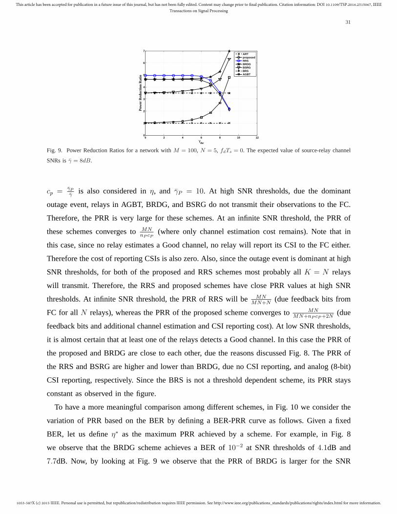
1053-587X (c) 2015 IEEE. Personal use is permitted, but republication/redistribution requires IEEE permission. See http://www.ieee.org/publications_standards/publications/rights/index.html for more information.
This article has been accepted for publication in a future issue of this journal, but has not been fully edited. Content may change prior to final publication. Citation information: DOI 10.1109/TSP.2016.2515067, IEEETransactions on Signal Processing
31
0 2 4 6 8 10 120
1
2
3
4
5
6
7
γthr
Pow
er R
educ
tion
Rat
io
ARTproposedRRSBRDGBSRGBRSAGBT
Fig. 9. Power Reduction Ratios for a network withM = 100, N = 5, fdTs = 0. The expected value of source-relay channel
SNRs isγ = 8dB.
cp = γPγ
is also considered inη, and γP = 10. At high SNR thresholds, due the dominant
outage event, relays in AGBT, BRDG, and BSRG do not transmit their observations to the FC.
Therefore, the PRR is very large for these schemes. At an infinite SNR threshold, the PRR of
these schemes converges toMNnP cP
(where only channel estimation cost remains). Note that in
this case, since no relay estimates a Good channel, no relay will report its CSI to the FC either.
Therefore the cost of reporting CSIs is also zero. Also, since the outage event is dominant at high
SNR thresholds, for both of the proposed and RRS schemes most probably allK = N relays
will transmit. Therefore, the RRS and proposed schemes have close PRR values at high SNR
thresholds. At infinite SNR threshold, the PRR of RRS will beMNMN+N
(due feedback bits from
FC for allN relays), whereas the PRR of the proposed scheme converges toMNMN+nP cP+2N
(due
feedback bits and additional channel estimation and CSI reporting cost). At low SNR thresholds,
it is almost certain that at least one of the relays detects a Good channel. In this case the PRR of
the proposed and BRDG are close to each other, due the reasons discussed Fig. 8. The PRR of
the RRS and BSRG are higher and lower than BRDG, due no CSI reporting, and analog (8-bit)
CSI reporting, respectively. Since the BRS is not a threshold dependent scheme, its PRR stays
constant as observed in the figure.
To have a more meaningful comparison among different schemes, in Fig. 10 we consider the
variation of PRR based on the BER by defining a BER-PRR curve as follows. Given a fixed
BER, let us defineη∗ as the maximum PRR achieved by a scheme. For example, in Fig. 8
we observe that the BRDG scheme achieves a BER of10−2 at SNR thresholds of4.1dB and
7.7dB. Now, by looking at Fig. 9 we observe that the PRR of BRDG is larger for the SNR

1053-587X (c) 2015 IEEE. Personal use is permitted, but republication/redistribution requires IEEE permission. See http://www.ieee.org/publications_standards/publications/rights/index.html for more information.
This article has been accepted for publication in a future issue of this journal, but has not been fully edited. Content may change prior to final publication. Citation information: DOI 10.1109/TSP.2016.2515067, IEEETransactions on Signal Processing
32
10−5
10−4
10−3
10−2
10−1
100
0
1
2
3
4
5
6
7
8
Bit Error Rate
Pow
er R
educ
tion
Rat
io
proposed
RRS
BRDG
BSRG
AGBT
BRS
ART
Fig. 10. BER-PRR curves for a network withM = 100, N = 5. The expected value of source-relay channel SNRs isγ = 10dB.
of 7.7dB (around5). Therefore, for BRDG at BER=10−2, we haveη∗ = 5 (this point does not
appear on Fig. 10 since in Fig. 10 we increase the expected value of source-relay channel SNRs
to γ = 10dB, whereas for Fig. 8 and Fig. 9 we haveγ = 8dB). In fact, the BER-PRR curve
defined here is similar to a Rate-Distortion curve, where PRR acts similar to the compression
ratio of a scheme compared to the ART scheme.
To obtain Fig. 10, as explained above, the BER and PRR curves are separately derived by
varying γthr and then are combined based on the above definition. Since ART and BRS are
not threshold based, their BER and PRR does not change withγthr. Therefore, in Fig. 10, their
performance is shown as single operational points. At BERs less than10−3, the proposed scheme
offers the largest value of PRR. For larger BER values, the BRDG offers the best PRR. These
two schemes (which are very similar to each other in nature) seem to offer the best BER-PRR
tradeoff. However, due to the no transmission during outage event, the BRDG is not able to
achieve very low BERs (as shown in the figure).
Figure 11 shows the BER-PRR curves of different schemes over time-varying fading source-
relay channels withγ = 6dB and fdTs = 0.002. The source block length isM = 128 bits
and the number of relays in the network isN = 5. A total of nP = 5 pilots are used for
channel estimation and the expected value of SNR for pilot symbols isγP = 10. Since only
the proposed, ART, RRS, and AGBT schemas are directly applicable to time-varying fading
channels, we compare the performance of these schemes. The curves are derived by varying
the SNR threshold between4dB and8dB. Since ART is not threshold-based, its performance
is shown as a single operating point. It is observed that the proposed scheme is able to achieve

1053-587X (c) 2015 IEEE. Personal use is permitted, but republication/redistribution requires IEEE permission. See http://www.ieee.org/publications_standards/publications/rights/index.html for more information.
This article has been accepted for publication in a future issue of this journal, but has not been fully edited. Content may change prior to final publication. Citation information: DOI 10.1109/TSP.2016.2515067, IEEETransactions on Signal Processing
33
10−4
10−3
10−2
10−1
100
0.5
1
1.5
2
2.5
3
3.5
4
4.5
5
Bit Error Rate
Pow
er R
educ
tion
Rat
io
RRSAGBTproposedARTproposed: perfect CSIAGBT: perfect CSI
Fig. 11. BER-PRR curves for a network withM = 128 and N = 5. The source-relay channels are time-varying with
fdTs = 0.002
BERs slightly lower than the one offered by ART. This is due applying the ML decoding as
explained in Section V. As observed from Fig. 11, the proposed scheme offers the best BER-
PRR tradeoff for BERs up to10−2. The dashed curves in Fig. 11 show the BER-PRR curves
for the proposed and AGBT schemes when perfect CSI is available at the FC. For evaluating
the PRR we still count the channel estimation cost,nP × cP . However, we assume that given
this cost, CSIs are perfectly estimated and delivered to the FC. We observe that both AGBT and
proposed schemes show a performance degradation due imperfect channel estimation. However,
this performance loss is more significant in the case of the proposed scheme. To justify this, note
that in the proposed scheme we use the bit reliabilities (pG, pB) for ML decoding. By incorrectly
estimating a Good bit as a Bad bit (or a Bad bit as a Good bit), we also provide the decoder
with mismatched reliabilities that will further degrade the BER.
In Fig. 12 the effect of co-channel interference (CCI) on the BER of the proposed scheme is
studied. To model CCI, we use a scheme from [36] where an external interfering source transmits
at the same frequency as the source sensor. The received signal at relayn is then modeled as:
y (n,m) = h (n,m) b (m) + h′
(n,m) b′
(m) + z (n,m) (39)
whereh (n,m) = α (n,m) ejθ(n,m) is the source-relay channel gain,h′
(n,m) = α′
(n,m) ejθ′
(n,m)
is the channel gain from interfering source to the relay,b′
(m) is the transmitted bit by the
interfering source, andz (n,m) is the AWGN term. The transmit power of the interfering
source is normalized to one, i.e.b′
(m) ∈ ±1. Following [36], we define a parameterL

1053-587X (c) 2015 IEEE. Personal use is permitted, but republication/redistribution requires IEEE permission. See http://www.ieee.org/publications_standards/publications/rights/index.html for more information.
This article has been accepted for publication in a future issue of this journal, but has not been fully edited. Content may change prior to final publication. Citation information: DOI 10.1109/TSP.2016.2515067, IEEETransactions on Signal Processing
34
where the power of interfering channel is1L
times the power of the source-relay channel,
i.e.E[
α′
(n,m)]
E[α(n,m)]= 1
L. As we discussed before, the source-relay channel phase is assumed to
be known at the relay. Therefore, by applying coherent detection, the detected signal at the relay
is r (n,m) = Re
y (n,m) e−jθ(n,m)
. We observe BER degradation due to the interference at
the relays. One approach to compensate for this degradation is to increaseαthr, which results
in more reliable Good bits and lower BER. However, by changingαthr, the parameters of the
Gilbert-Elliott channel (µ, ǫ) will change and therefore; the distribution of the selected subset size
will change. This results in a change ofE [K] and consequently a change of PRR. Therefore,
to fairly study the effect of this BER compensation, one needs to compare the BER-PRR curves
for both the compensated and non-compensated schemes. A proper compensation coefficient for
αthr is found by noting that the maximum power of interference is1L
and the power of AWGN
is N0
2= 1
2γ. In other words, by adding the interference, the Signal-to-Interference-plus-Noise
Ratio (SINR) will be 11L+ 1
2γ
, whereas for the case of no interference only the power of noise
is present (i.e. the term112γ
). The ratio of these values isτ = 2γL+ 1. To compensate for this
SINR degradation, we may multiplyαthr by√τ . This will increase the expected value of SINR
for Good bits by a coefficientτ . Note that applying this compensation coefficient at the relay
requires the knowledge ofL, i.e. the interference power. It may seem impractical to assume that
the relay could estimate the interfering channel coefficient,h′
(m,n). However, estimation ofL
seems practical and is suggested in previous works including [37].
In Fig. 12 the value ofαthr (before compensation) is set to1 and the BER is evaluated for
various values ofγ. Both cases of perfect source-relay CSI, and imperfect CSI (nP = 5) are
considered. We observe that CCI compensation is more effective at lower values ofγ where the
Gaussian noise power is more dominant. At higher values ofγ, the noise power decreases and
the effect of CCI on the SINR is more significant. In this case, the suggested CCI compensation
is not very effective. Perhaps, for large values ofγ where the interference is dominant, we must
pay attention to the actual distribution of the CCI and design our compensation method based
on these statistics. Among references that study the distribution of CCI, we could refer to [38]
and references therein.
VIII. C ONCLUSION
We analyzed a two-hop WSN where source-relay channels are modeled as quantized time-
varying fading channels (Gilbert-Elliott channels). We proposed a two-phase transmission scheme

1053-587X (c) 2015 IEEE. Personal use is permitted, but republication/redistribution requires IEEE permission. See http://www.ieee.org/publications_standards/publications/rights/index.html for more information.
This article has been accepted for publication in a future issue of this journal, but has not been fully edited. Content may change prior to final publication. Citation information: DOI 10.1109/TSP.2016.2515067, IEEETransactions on Signal Processing
35
3 4 5 6 7 810
−5
10−4
10−3
10−2
γ (dB)
Bit
Err
or R
ate
No CCI, perfect CSINo CCI, n
p = 5
L=10, perfect CSI, CCI compensationL=10, n
p = 5, CCI compensation
L=10, perfect CSI, no CCI compensationL=10, n
p = 5, no CCI compensation
Fig. 12. Effect of Co-Channel Interference on the BER achieved by the proposed scheme.M = 128, N = 5, andfdTs = 0.002.
where at the first phase compressed channel state information sequences are transmitted to the
FC and a subset of sensors are selected to transmit their observations to the FC at the second
phase. We analytically derived the probability distribution of the size of the selected subset and
the expected value of this subset size. We presented simulation results to assess the performance
of our scheme compared to schemes appearing in literature. Our simulation results showed
that for a certain range of end-to-end BERs, the proposed scheme achieves a superior power
reduction compared to other schemes. Extension of the presented analyses for the case of noisy
relay-FC channels seems an interesting topic for future research in this direction. Analyzing the
system behaviour when relays work in full-duplex mode is another interesting problem for future
research. In this case, the Gilbert-Elliott model has to be modified to take the interference of
relays on other relays into account.
ACKNOWLEDGMENT
The authors would like to thank the editor and anonymous reviewers for their insightful
comments. The second author also acknowledges fruitful discussions with Prof. Mohsen Eslami.
REFERENCES
[1] I. F. Akyildiz, W. Su, Y. Sankarasubramaniam, and E. Cayirci, “A survey on sensor networks,”IEEE Communications
Magazine(2002), Pages: 102-114.
[2] Chin-Liang Wang, Syue-Ju Syue, “An Efficient Relay Selection Protocol for Cooperative Wireless Sensor Networks,”
Wireless Communications and Networking Conference, 2009. WCNC 2009. pp.1-5, April 2009.

1053-587X (c) 2015 IEEE. Personal use is permitted, but republication/redistribution requires IEEE permission. See http://www.ieee.org/publications_standards/publications/rights/index.html for more information.
This article has been accepted for publication in a future issue of this journal, but has not been fully edited. Content may change prior to final publication. Citation information: DOI 10.1109/TSP.2016.2515067, IEEETransactions on Signal Processing
36
[3] Zorzi, M.; Rao, R.R., “Geographic random forwarding (GeRaF) for ad hoc and sensor networks: multihop performance,”
Mobile Computing, IEEE Transactions on, vol.2, no.4, pp.337,348, Oct.-Dec. 2003
[4] X.J. Zhang and Y. Gong, “Joint power allocation and relay positioning in multi-relay cooperative systems”,IET Commun.
(2009), vol. 3, Issue: 10, Pages:1683-1692.
[5] Ranhotigamage, C., Mukhopadhyay, S.C., “Field Trials and Performance Monitoring of Distributed Solar Panels Using a
Low-Cost Wireless Sensors Network for Domestic Applications,”Sensors Journal, IEEE, vol.11, no.10, pp.2583,2590,
Oct. 2011
[6] Mahmut Karakaya, Huirong Qi, “Target detection and counting using a progressive certainty map in distributed visual
sensor networks”International Conference on Distributed Smart Cameras,ICDSC 2009, Pages: 1-8.
[7] Zhang Ke, Li Yang, Xliao Wang-hui, Suh Heejong, “The Application of a Wireless Sensor Network Design Based on
ZigBee in Petrochemical Industry Field”International Conference on Intelligent Networks and Intelligent Systems, ICINIS
2008, Pages: 284-287.
[8] T. Wang, R. C. de Lamare, P. D. Mitchell, “Low-complexity set-membership channel estimation for cooperative wireless
sensor networks,”IEEE Transactions on Vehicular Technology, Vol. 60, N0. 6, July 2011, Pages: 2594-2607.
[9] G. Anastasi, M. Conti, M. Di Francesco, A. Passarella, “Energy conservation in Wireless Sensor Networks: A Survey,”
Elsevier Ad Hoc Networks,7 (2009) 537-568.
[10] V. Raghunathan, C. Schurghers, S. Park, M. Srivastava, “Energy-aware wireless microsensor networks,”IEEE Signal
Processing Magazine(2002) Pages: 40–50.
[11] G. Pottie, W. Kaiser, “Wireless integrated network sensors,” Communication of ACM 43 (5) (2000) 51–58.
[12] E.N. Gilbert, “Capacity of a burst-noise channel,”Bell Syst. Tech. J., vol. 39, no. 9, pp. 1253–1265, Sept. 1960.
[13] E.O. Elliott, “Estimates of error rates for codes on burst-noise channels,”Bell Syst. Tech. J., vol. 42, no. 5, pp. 1977–1997,
Sept. 1963.
[14] P. Sadeghi, R. A. Kennedy, P. B. Rapajic, and R. Shams, “Finite-State Markov Modeling of Fading Channels,”IEEE Signal
Processing Magazine,Sep. 2008, pp. 57-80.
[15] N. Khajehnouri, A. H. Sayed, “Distributed MMSE relay strategies for wireless sensor networks,”IEEE Transaction on
Signal Processing, Vol. 55, No. 7, July 2007, Pages: 3336-3348.
[16] A. Willing, “Recent and emerging topics in wireless industrial communications: A selection,”IEEE Transactions on
Industrial Informatics,vol. 4, n0. 2, pp. 102-124, May 2008.
[17] Sheryl L. Howard, Christian Schlegel, and Kris Iniewski, “Error control coding in low-power wireless sensor networks:
When is ECC energy efficient,”EURASIP Journal on Wireless Communications and Networking, pages 1–14, 2006.
[18] M. R. Islam “Errorcorrection codes in wireless sensor network: An energy aware approach,”Int. J. Comput.Inf. Eng., vol.
4, no. 1, pp.59 -64 2010
[19] Abedi, A., “Power-efficient-coded architecture for distributed wireless sensing,”Wireless Sensor Systems, IET, vol.1, no.3,
pp.129,136, September 2011
[20] K. Yu, F. Baracy, M. Gidlundz and J. Akerbergz, “Adaptive forward error correction for best effort wireless sensor networks,”
IEEE International Conf. on Communications (ICC), Ottawa ,June 2012, pp. 7104-7109.
[21] W. C. Jakes,Microwave Mobile Communications, New York: IEEE Press, 1974.
[22] X. Li, “Blind channel estimation and equalization in wireless sensor networks based on correlations among sensors,”IEEE
Transactions on Signal Processing, Vol. 53, No. 4, April 2005, Pages: 1511-1519.
[23] J. Gao, H. Liu, “Decision-directed estimation of MIMO time-varying Rayleigh fading channels,”IEEE Trans. Wireless
Communications, Vol. 4, No. 4, July 2005, Pages: 1412-1417.

1053-587X (c) 2015 IEEE. Personal use is permitted, but republication/redistribution requires IEEE permission. See http://www.ieee.org/publications_standards/publications/rights/index.html for more information.
This article has been accepted for publication in a future issue of this journal, but has not been fully edited. Content may change prior to final publication. Citation information: DOI 10.1109/TSP.2016.2515067, IEEETransactions on Signal Processing
37
[24] A. Wiesel, “SNR estimation in time-varying fading channels,”IEEE Transactions on Communications, Vol. 54, No. 5,
May 2006, Pages: 841-848.
[25] H. Abeida, “Data-aided SNR estimation in time-variant Rayleigh fading channels,”IEEE Trans. Signal Processing, Vol.
58, No. 11, November 2010, Pages: 5496-5507.
[26] F. Bellili, R. Meftehi, S. Affes, A. Stephenne, “Maximum likelihood SNR estimation of linearly-modulated signals over
time-varying flat-fading SIMO channels,” IEEE Trans. Signal Processing, Vol. 63, Issue: 2, Jan. 2015, Pages: 441-456.
[27] C. Bonferroni, “Teoria statistica delle classi e calcolo delle probabilita,” Pubbl. d. R. Ist. Super. di Sci. Econom. e
Commerciali di Firenze(in Italian), vol. 8, Pages: 1–62, 1936.
[28] S. S. Ikki, S. Al-Dharrab, M. Uysal, “Error probability of DF relaying withpilot-assisted channel estimation over time-
varying fading channels,”IEEE Transactions on Vehicular Technology, vol. 61, No. 1, Jan. 2012.
[29] C. K. Lo, S. Vishwanath, R. W. Heath, Jr., “Relay subset selection in wireless networks using partial decode-and-forward
transmission,”IEEE Transactions on Vehicular Technology, vol. 58, No. 2, Feb. 2009.
[30] I. Ahmed, A. Nasri, D. S. Michalopoulos, R. Schober, R. K. Mallik, “Relay subset selection and fair power allocation for
best and partial relay selection in generic noise and interference,”IEEE Transactions on Wireless Communications, vol.
11, No. 5, May 2012.
[31] E. Beres, R. Adve, “Optimal relay-subset selection and time-allocation in decode-and-forward cooperative networks,”IEEE
Transactions on Wireless Communications, vol. 9, Issue: 7, July 2010.
[32] I. Krikidis, J. S. Thompson, S. McLaughlin, N. Goertz, “Max-min relay selection for legacy amplify-and-forward systems
with interference,”IEEE Transactions on Wireless Communications, vol. 8, No. 6, June 2009
[33] A. Bletsas, A. Khisti, D. P. Reed, and A. Lippman, “A simple cooperative diversity method based on network path
selection,”IEEE J. Sel. Areas Commun., vol. 24, pp. 659–672, Mar. 2006.
[34] L. Ahlin, “Coding methods for the mobile radio channels,”Nordic seminar on digital land mobile communications, Feb.
1985, Espoo, Finland.
[35] H. Mheidat, M. Uysal, “Non-coherent and mismatched-coherent receivers for distributed STBCs with amplify-and-forward
relaying,” IEEE Transactions on Wireless Communications, vol. 6, no. 11, pp. 4060-4070, Nov. 2007.
[36] I. Krikidis, J. S. Thompson, S. McLaughlin, N. Goertz, “Max-min relay selection for legacy amplify-and-forward systems
with interference,”IEEE Transactions on Wireless Communications, vol. 8, no. 6, June 2009, pp. 3016-3027.
[37] N. Suraweera, N. C. Beaulieu, “The impact of imperfect channel estimations on the performance of optimum combining
in decode-and-forward relaying in the presence of co-channel interference,”IEEE Wireless Communications Letters, vol.
3, no. 1, Feb. 2014, pp. 18-21.
[38] K. Gulati, B. L. Evans, J. G. Andrews, K. R. Tinsley, “Statistics of co-channel interference in a field of Poisson and
Poisson-Poisson clustered interferences,” IEEE Transactions on Signal Processing, vol. 58, no. 10, December 2010, pp.
6207-6222.