analysis of integrated voice and data communication
TRANSCRIPT
ANALYSIS OFINTEGRATED VOICE AND DATA
COMMUNICATION NETWORK
Lih-Hsing Chang
Department of Electrical EngineeringCarnegie-Mellon University
Pittsburgh, Pa.15213
November 1977
This work was supported by Defense Comunication Agency under contract number(DCA 100-76-0058).

ABSTRACT
This thesis studies the performance of an integrated voice and data
communication network. Different characteristics from other communication networks
and a different set of key parameters for its performance are addressed. The
relationship of and the trade-off between the key parameters are also discussed.
Voice communication requires slow but continuous information e×change while
data communication requires burst type of information exchange. A new integrated
switch is designed to support both type of communications_ line switch for voice and
packet switch for data. Class ] traffic, voice or video, is modeled as an M/M/n queue
and Class lI traffic, data or bulk, is modeled as an M/M/Y queue. A wild distribution of
Class [I queue length is discovered and a significant trade-off between communication
and ccmputer facilities is implied. The study shows that the queue length grows very
rapidly when the Class ]/Class ]] job size ratio increases. A small integrated switch
with relatively small job size ratio is studied in details. However large switches with
realistcal job size ratio are only approximated and detail quantitative results for such
system require further study.
The longer the queue is, the larg;er the memory will be required to store the
data packets. However though the integrated switch has a very long queue, the
number of buffer for the switch to operate efficiently is rather limited as shown by
the network queueing model. In order to increase the memory utilization and to lower
the system cost, several memory management and buffer assignment schemes are
discussed, An unconventional secondary storage for switching processor is modeled
and the advantages and disadvantages are thoroughly discussed.

A special delay of integrated switch is introduced by its frame structure. In,
order to minimize the through network delay, the design problem of how to share the
. communication link capacities between voice and data and how to assign the frame
skew on each link are discussed. Because of discrete delay incremented by the frame
period, the frame skew assignment problem is investil]ated as a mixed integer linear
program. A speeding algorithm using k-tree concept is developed to speed up the
ordinary branch and bound algorithm. However the speedin_ algorithm does not show
much improvement in computation time and is thus limited useful. A heuristic algorithm
is then developed to find a local optimal assis;nment in relatively short computation
time.
TIT

ACKNOWLEDGEMENT
o
First and foremost my thanks go to my advisor, Professor Sam Fuller, for his
enli6htened supervision of this work, and to the other members of my committee,
Professor Dan Sieworek, John Lehoczky and Dr. Mario Barbacci for readin6
innumerable version of the draft and for givins; thoug,htfui comments.
! am further indebted to the DCA group whom | have worked with and received
various comments and sugsestion from for the past two years.
I like to give thanks to all my friends who gave me so many help and
encourat_ement during the past several years. Special thanks go to Mr. Chert and
Mr.Tun6 who host me when I come back to finish this work.

T A B L E P F ,,,C_,0,I_ T E _ T S
ANALYSIS OF
INTEGRATED VOICE AND DATA COMMUNICATION NETWORK PAGE
CHAPTER 1 Introduction
I.i Computer Communication....................... I[
1.1,1Line-SwitchedNetwork ....................
i,1.2 Message-SwitchedNetwork .................
1.1,:3IntegratedSwitchedNetwork ................ 7
1.2 SENET Configuration .................... " • • 9
1.2.1Frame ............................. 9
1.2.2ServiceRequirements ................... 11
I.:3 PreviousWork ........................... 1A
1.4 Synopsis of Thesis ........................... 17
......
CHAPTER2 Performance Analysis___
2.1 Introduction ............................... 19
2.2 Models ................................ 21
2.2.1 Integrated Switch Model .................... 21
2.2.2 Models ............................. 23
2.2.3 Comparison .......................... 27

2,3 ]nte_;rated Swilch Model .... ................... ,32
2.3.1 Class ! Jobs .......................... 33
2.3.2 Class II Jobs .......................... 3/'1•
2.3.3 Multi-Server Model ....................... 4,6
2,4 Error Analysis and Conditional Mean Approximation .......... 50
2.4.1 Error Analysis ....................... 50
2.4.2 Conditional Mean Approximation ................ 53
2.5 Diffusion Approximation ....................... 56
2.5.I Time-Dependent System .................... 56
2.5.2 Simple Diffusion Model .................. 60
2.5.3 Diffusion Approximation for the Integrated Switch ....... 66
2.6 Comparison of Results ........................ 68
CHAPTER 3 Memory Mazmgement for Dal;a ButTers
3.1 Introduction ............................. 77
3.2 Node Model ............................. 80
3.2.1 Maximum Size Buffers .................... 80
.3.2.2 Different Fixed Size Buffers ................. I 831
3.2.3 Dynamic Memory' Allocation ................ 96
I
3.3 Network Model .......................... I 100
3.3.1 Exponential Queueing Network ................ 101
3.3.2 Queuein 8 Network with Time Lag ................ 106
vl'

3.3.3 Numerical Results ....................... 109
3.4 Secondary Storage Model ................ ....... XX2
z133.4.1 Modeling ...........................
3.4.2 Forward and Backward Aisorithm ............. _,16
3.4.3 Numerical Results ....................... 120
_ 1283,5 Conclusion ............................. I
CHAPTER 4 SE]tET NeWork Design
4.1 Introduction . . . ........................... 129
4.2 The Model .............................. 131
4.2.1 Variables .......................... 131
4.2.2 PerformanceMeasures .................... 133
4.2.3 DesignProblems ....................... 136
4.3 Capacity Assignment Problem ..................... 138
4,3.1 Small Frame Capacity Assignment ............. 138
4.3.2 General Capacity Assignment ................ 143
I 1494.4 Frame Skew Assignment Problem ................... i
4.4. i Formulation .......................... 149
4.4.2 Branch and Bound Algorilhm .................. 130
4.4.3 Acceleratin 8 Algorithm .................... 1.5/4,
vll

4.5 Heuristic AIl_orithm ........................... 159
4.5.1 Cuts and Trees ........................ i159}
4.5.2 The AII]orithm 165
CHAPTER 5 Conclusion
5.1 Interpretation of Results ....................... 169
5.2 Directions for Future Research .................... 172
viii

CHAPTER 1 Introduction
1.1. Computer Communication
The computer communication fietd is some 20 years old now, having originated
with military commanct and control system in which widely dispersed radar inputs and
outputs to weapon sites had to be controlled rapidly and in real time by a central
facility. That central facility could only be a digital computer because of the speed and
data volume involved. Today, data-processing systems having a communications
network as an integral "central nervous system" are a growing part of our daily lives.
These data processing systems are evolving at a bewildering speed and in a variety of
directions. Their evolution is made possible by new hardware and software
developments, new user needs, and new transmission systems tailored to computer
communication.
During much of the 1960s, the growth of computer networks was hampered by
the lack of communication facilities well suited for data transmission. Because the
existing telecommunication networks designed and operated by commerical carrier.,; had
evolved in a manner conducive to voice communications, they could not readily provide
the switching functions needed for the overall cost effective utilization of transmission
facilities for interactive data communications. As a result, we witnessed an emergence
of special networks such as DATRAN, ARPANET, and others dedicated to data users.
Today separate packet switching networks are used widely for data communications.
Although there appear to be valid justifications for the above trend, the practice
of separating voice and data traffic should be continually examined. The search for

switching approaches that would allow more versatility with respect to answerin£, all
• communication needs should be encouraged. In this thesis we will take a took at a
single communication network which provides both data and voice traffic services
throup_,h the use of a switching approach that operates somewhere between a full
circuit-switched and a full packet-switched concept.
As shown in fiF_,ure 1.1.1, a computer communication network usually consists of
terminals, local loops, switching centers (SC), and hip_,hspeed trunks, which form the
backbone communication system. A terminal may be a teletype, a telephone or a
computer. A message generated by a terminal is transmitted by local loops to a
switching center. From the switching center, the messag;e is carried by a hig;h speed
trunk, in exactly inverse order, to the destination terminal.
o TRUNKo
o
o
TERNINAL
FIGURE I. 1.1 COMPUTER CO_[MUNICATION NETWORK
There are basically two kinds of switching techniques, line-switching: and
message-switchin 6. The dial telephone system is a typical line-switched system, while

the telegraph system is a message-switched system. Brief descriplions of a line-
switched network, a message-switched network, and the new integrated switched
network, a mixture of line and message switching, follow.
I.I.I.Line-Switched Network
tn a line-switched system, information from a sending terminal is not transferred
to a receiving; station until the network has set up a connection. As figure 1.1.2
shows, a terminal starting a call submits a "send request" to the exchange, where
further dialing information is started. The nodal control processor generates; an
inquiry signaling message. This inquiry message precedes, link by link, to the
receiver's exchange. There, a response message which reflects the status of the
rec:eiver desired is prepared. The response proceeds, again, link by link.-.= o. • • . 4, • • . o ,,=, =. ." -o .
• r •o .
. " szNo III-""INQUIRY • II _NQU_RYIII " •
RESPONSE " : :. ;
11 ill LDISCONNECT " "
DOWN MESSAGE MESSAGE • .
o
FIGURE 1.1.2 LINE-SWITCHED NETWORK
There are two possible ways to set up the path. Tile first is the forward path
set-up, in which the inquiry message causes the nodal processors to connect the links

of the path from the sender to the receiver exchange, without the knowledge of the
receiver status. The second is the backward path set-up which is initiated by the
response messaBe when the receiver is available.
In both instances, when the path is completed, a "start-to-send" message is sent
to the sender by the sender's switching center. Release of a path is initiated by a
"clear-down"command. During these two control signals, the path is reserved for this
connection, and the switchin 6 processor, which is not affected by presence or absence
of information flowin_ on the path, will not intervene.
In line-switched networks, sil_naling messages may be exchanged between nodes
in two ways: via a special, common signaling channel exclusively dedicated to the
transfer of network signaling messages, or over the same channel which also conveys
the customer message (individual or separate signalin_ ctlannel system). The latler
automatically implies the forward path set-up from the sender to the receiver.
In principle, path establishment in a line-switched network is a store-and-
forward process. Customer message transfers are always preceded and ended by a
store-and-forward signaling phase.
1.1.2. MessaRe-Switched Network
In a message-switched system, messages are temporarily stored in the nodes.
Messaooe transfer involves three steps: from the sender to his switching center,
between switching centers, and from the destinalion switching center to the receiver.
Figure t.1.3 shows the typical signaling procedure. Customer messages are routed to
the destination node with the help of address information contained in a header tagged
to the message. It is assumed that the receipt of a message is signaled by an
4

acknowledgement message. Two kinds of network signaling messages can thus be
distinguished' headers and pure signaling messages, such as acknowledgements.
, °.- .- _ . .
..... "" = " "-: FIGURE 1.1.3 MESSAGE-SWrrCHED NETWORK '• . . ".
• "" . .-. * :[ . . .., .. •. . . ..
- ,... ..
Figure 1.1.4 shows the transfer delay of a line-switched network, and a
message-switched network. When the transmission time of customer messages over
the path is long compared to the connect and disconnect time, line-switching is
preferable. Line-switching has comparatively little overhead, because it does not need
the large buffer space required for message-switching. On the other hand, when the
size of the messages decreases, the overhead of line-switching increases, making
message-switching preferable, since the total signaling of path connection for ]line-
switching has more overhead than a node by node, store-and-forward message
transmission. As long as the buffer space for message-switching is not too large,
message-switching is more cost effective.

TRANSMISSION OFCONNECT CUSTOMER MESSAGE DISCONNECT
• TIME . OVER PATH TIME
' i 1 1 ....• _ t
"'' LINE-SWITCHED NETWORK
• .
TRANSM. OF TRANSFER OF TRANSM. OFLOCAL- CUSTOMER MESSAGE CUSTOMERMESSACE _"_T_"_n,'_-_LOOP OVER SENDER THROUGHHIGHLEVEL O_R_T3_.__!\.);_;........
SIGNALING LOCAL LOOP NETWORK LOCAL-LOOP
I I I I I-'MESSAGE-SWITCH NETWORK • ! "
-- _. ,°..
• 'f_IGURE 1.1.4 TIMING CONFIGURATION•
There is a variation of the message switching technique called packet-switching.
Packet-switching function and control properties are the same as those of message
switching, but there is an upper limitation on the size of packets.
A message that is too large for a packet is broken into several packets, each
with its own destination and sending information. The disadvantage of packet-
switching is that it involves more overhead than ordinary message-switching. Instead
of one overhead message header per a message, there are several packet header
containing similar addressin_ information. The advantages of packet-switching are
smaller buffer size requirement and more flexible flow control. ARPANET and AUTODIN
are two of the many large resource sharing networks using pack,el-switching
technique.

1.1.3. ]nteF,rated _witched Network
The trends of future requirements for digital communication systems indicate an
increasin_ diversity of traffic characteristics such as:
(i). wide disparities between traffic rates, ranging from low-rate TTY terminals,
requiring hundreds of bits/sec, to wideband video and graphics terminals, requiring
hundreds of kilobits/sec.
(ii). wide disparities in transaction sizes, starting with interactive messages of
several hundreds of bits and continuing up to bulk data transfers of millions of bits.
(iii). varying delivery times to accomodate voice and video, which requires
continuous, near real-time response; interactive data terminals, which require response
time in the order of seconds; and bulk data, which can be queued for hours.
From the description of the traffic requirements, it is clear that no single
switching technique can give satisfactory response to all requests. A line-switched
network will have tremendous overhead, or waste, on a communication facility designed
for interactive data requisition. A simple calculation by James Martin [Mart 72] shows
that only 0.1'7. of the total communication facility is used when a teletype is connected
to a computer through a telephone line. Telephone systems use line switching, while
the data generated by a teletype is a sequence of bursts, which is ideal for message-
or packet- switching. On the other hand, neither message- nor packet- switching can
handle voice communications or wideband video signals wilh the response time needed
to maintain the integrity of the information. Because they posses sufficient
redundancy, voice or video signals are not sensitive to the error rate of channels.
Timing, however, is very critical, often in the order of tens of milliseconds of total path
delay, and il is very difficult for a message-switched network,, with its error detection
and acknowledgement mechanisms, to meet such demands.
?

In order to use communication facilities more efficiently, it is nature to suggest
the mersin 6 of different switching techniques into one network. Recently, several
efforts [For8 75, Covi 75] have been made to define di_,ital communication_ schemes in
which the network capacity is shared between a line-switched and a messaEe-swilched
system. Such schemes allow the most efficient and appropriate switching technique to
be chosen for each service request. Almost all these schemes need more processing,
power than that providod by tho conventional network switching. However, as
processor and memory costs continue to decline faster than transmission costs_ an
integrated switch becomes feasible and cost effective.

1.2. SENET Confi_,uration
SENET (Slotted Envelope NETwork)is a proposed scheme for an integrated
switching network. The idea is suggested by Coviello and Vena [Covi 75], and its
implementation is discussed in [Barb 76] in more detail. SENET is a Time Division
Multiplex (TDM) scheme in which time slices of fixed size, a frame period, are
partitioned and allocated to the transmission of digitized voice and data packets. The
voice component of a frame is further divided into slots allocated to ongoing line
switching communications. Slols reserved along a path on the network establish a
virtual line-switch path between the end subscribers.
This scheme can handle three different types of traffic.
Class 1. Characterized by long transactions requiring continuous real time
response (voice, video, facsimile). The transmission rate may vary from thousands of
bit/sec (voice) to hundreds of thousands bits/sec (video).
Class ]I. Characterized by short discrete transactions requiring near real time
response (interactive data, with data requisition being the typical example). The
response should occur within seconds.
Class IlL Characterized by long transactions requiring neither continuous nor
immediate response (bulk data).
1.2.1o Frame
The detail of a frame is shown in figure 1.2.1. Starting at the 12 o'clock
position, a certain number of bits are reserved for CCIS (Common Channel Interswitch
Signaling). Following this region is a Class I region containing the real time traffic. The

START MARKER
CCIS
Class III TrafficPacket Switched
Voice Class I Traffic
Bulk Circuit Switched
_ Voice
Video
• Data
ice
Class 11 Traffic
Packet Switched Data oice
DataBOUNDARY MARKER
FIGURE 1.2. I INTEGRATED SWITCHED NETWORK FRAME
10

end of the Class I region is indicated at 5 o'clock. Class ]] and Class II[ regions
containing the interactive and bulk traffic respectively occupy the rest of the frame.
All the interactive data or bulk data are transmitted inside the Class I[ region in
disjoint packets. (For most of the thesis, we shall make no distinctions between Class l[
and Class [[[ traffic. Unless we explicitly indicate otherwise, we will use the term __:las__._ss
L[ to indicate both interactive data and bulk data transmitted by packet switching.) Real
time traffic, on the other hand, is transmitted inside the Class I region in fixed slots,
with one slot allocated for each logical channel currently in use.
The scheme does not assume the existence of a master network clock. Each link
• transfers frames at a constant rate, but the links are not necessarily synchronized
among themselves. Frame timing for each link is discussed in Chapter 4. In addition,
the network does not require a homogeneous link of the same speed. For a given
frame period, say 10 milliseconds, the number of bits contained in the frame depends
on the speed of the link. Thus, for a T1 carrier, a lO-miilisecond frame contains 15,440
bits, while for slower carrier, a iO-millisecond frame is smaller.
1.2.2. Service Requirements
Eachof the three types of traffic requires different type of service. Class I is
either accepted or rejected, with short connection delays and without error conti'ol. It
represents a loss system in which there is a small probability of a connection being
refused if no logical channel can be established between subscribers. CZass ! traffic
requires low delay and a constant throughput in order to maintain the intelligibility of
the message. Class II traffic is always accepted, but it may incur a system delay with
short cross-network delay and reasonable response time. This traffic is characterized
11

by bursts of information followed by "waiting" periods, requiring hiBh deg;ree of
reliability. Class ]|! traffic is always accepted with longer cross-network delay than the
previous class. Class I[ traffic also requires a high degree of reliability.
The real time requirements of Class ! traffic dictate that it be processed in
special fashion by the integrated switch. Since voice or video siBnals carry a
significant amount of redundancy, a moderate error rate can be tolerated in most
applications. Elimination or reduction of the need for error control enables Class !
traffic to be transmitted in a straightforward manner. The establishment of a logical
path between two subscribers is reflected, on each switch along the path, by the0
updating of Class ] Routing Tables internal to the integrated switches. These tables
indicate, for each slot in the Class I region of an input frame, both the output frame
(output channel) and the slot position reserved for the logical path.
Entries in the Routing Table are reserved according to the connecting request in
the line switched system. The inquiry control messages proceeds, link by link, to the
receiver. These messages also carry information about the data rate, slot size, and
priority of the logical channel. The reservation of the slots along the communication
path guarantees a fixed bandwidth for this type of traffic. The common characteristics
of this type of traffic are : (i)long holding, time, which is defined as the duration
between the commands of connection and disconnection and is in the order of minutes,
(ii) relatively less bits/frame compared to the size of one Class |[ packet which is
always transmitted within one frame. Typically Class I slots require a few hundred of
bits/frame, while Class |[ packets require ill the order of thousand bits/frame.
The communication facility is divided into frames, but the transmission and the
receiving of Class ]| traffic are packet oriented. The control functions, error checking,
12

buffer assiBnmont, and acknowted_,ernent Benerating are independently processed for.
each packet. The processor (or processors) assigns packet buffers to each incoming
packet and copies the packets into the buffers, after an input frame has been
completely written in the input frame buffer. In packet switchin B, at least one goad
copy of the data packet must exist in the ccmmunication system. For every correctly
received packet, an acknowledEement is echoed back to !he sender, so that the copy
of the packet still at the sender can be released. The same philosophy applies to the
integrated switch: A buffer will be released only if the packet is sent out to the ne×t
node and a positive acknowledgement of the packet is echoed back. The frame buffer
is ready to accept a new input frame after copyint_ the data packets into buffers and
copying the voice slots directly into the corresponding; output frame. In the meantime,
various tasks such as error checking, routing, and controlling are processed on a per
packet basis.
t3

1.3. Previous Work
A considerable amount of research has been done during the last decade in the
field of computer-communication networks. This research covers areas such as
modeling, analysis, design, data evaluation, and measurement for the whole network
and also for the communication processors.
A separate data-communication device for computers is considered after the
development of large multi-access systems when the data traffic became crowded.
Initially, the access terminals were few and close and the communication costs were
not an important factor. The system needs a multiplexer and a demultiple×er to get
efficient data access and good response time. The behavior of a local communication
network is discussed by Chu [Chu69, Chu72].
The sharing on larse data bases results in many terminals relatively far away
and the communication costs gradually became dominant. There are two _,eneral
models of a centralized computer-communication systems: the star network [Do169] and
the loop network [Pie72]. The data or requests to and from the terminals are no
longer sent without any identification. The information is packed into packets or slots.
The multi-drop line system [Cha72b] and ring switched data transmission system
[Gra71, Hay71] are two typical examples. There is a header for each packet which
contains sender and destination addresses and sometimes other control information.
For the more sophisticated switching functions, semi-independent or totally'
independent front-end processors are used rather than the hard wired multiplexers.
Chang [Cha72a] presents a typical design and evaluation of such communication
processors.
14

In order to achieve resource sharing in a lar£,er scope [Rob70], instead of the
communication between computer and terminals, the need of communication between
computers ari6es, The problem of packet routing arises in such communication system_;
along with other control functions and procotols. A totally independent communication
backbone system is implemented by communication processors. The ARPANET IMP
[Hea70] is an example of an independent switching processor. Modeling the IMP as a
queue server is quite successful for the analysis of the whole network. Both infinite
queueing space and finite queueing space have been analyzed [Kle74a, Kle74b, Meii71].
As the cost of the processing power and memory decline more rapidly than that of the
communication facility, the integration of the voice communication system becomes
feasible and cost effective. The ideas of such exposition are discussed by Forgie and
Coviello [For75, Cov75]. The implementation of an integrated switch has been tried on
a multi-processor system [CMU75, Bar76] and in an associate processing system
[Wa174].
The two different natures of voice and data make the analysis of an integrated
switch very difficult. Kummerie [Kum744] used an approximation technique to descril)e
the behavior of integrated switch. Later Bhat and Fischer [Bha75, Fis75] modeled the
system as a pre-emptive multi-channel system. The number of simultaneous equations
to be solved in the algorithm grows in the order of s(s+t)/2, where s is the number of
channels. In Chapter 2, we model the system another way, and the number of
simultaneous equations grows only in the order of s. A diffusion approximation
technique is used in the same chapter. This technique has been used in many
complicated queueing networks, [Fe166, Kob74a, Kob74b, Gay68]. The power of
diffusion approximation for the time-dependent system is especially described by
Gaver .[Gav68_
15

The buffer behavior was discussed by Chu[Chu69, Chu72] in the early sta_e of
muiliplexer type communication processor systems. Later studies on packet-swiiching
have dealt with the problem of packet size, buffer assis;nment, and the procotol of
packet flow [Whi70, Rud72, Chu73, C1o73, Ros75]. Queueing network analyses were
also undertaken. Gordon and Newetl [Gor67]discovered the product form steady state
distribution of a closed queueins, network with exponential servers. Later Baskett et al
[Bas75] extended this product form to more complicated networks: open , closed, or
mixed, with different classes of customers. The service time may also have a more
generalized distribution under some service disciplines, e.g. service time of rational
Laplace Transform for processor sharing servers. The algorithm to calculate the
product form solution is derived by Buzen [Buz73]. For more general service
distr:ibution, Chandy et al. [Cha75a, Cha75b, Her75"} developed an approximation
als,orithm using; Norton's theorem in electrical circuit theory. The analysis of closed,
finite queueing networks with time lags was introduced by Posner[Pos68].
The problem of the network desiF_n was first studied by Kleinrock [Kle72]. The
optimal capacity assisnment problem was analytically solved for the linear link cost
case. The criterion used was the total average waiting time. Meister et al. [Mei71]
solved the problem with a different crilerion: minimization of the total averase of kth
order of the waiting time. Using dynamic proF_,ramming: techniques, Frank et al. [Fra71]
solved the discrete capacity assiF,nment for a centralized S/F (Store and Forward)
network. An exact, but very cun_bersome, LP solution to the deterministic routing
problem is proposed by Frank et al. [Fra72]. The same problem was solved more
efficiently by Cantor et ai. [Can72], who used decomposition techniques. The difficult
problem of simultaneous routint_ an¢t capacities assignment was approached, with
mathematical prot_ramming techniques, by Gerla [Ger73].
16

1.4. Synopsis of Thesis
This thesis emphasizes the special SENET implementation of the integrated
switch. An important characteristic of the integrated switch is that the voice holding
time is much longer than the data packet service time. Because of this property, the
waiting length of data packets will vary greatly under different loading of voice c_Jls.
This phenomenon is discussed in Chapter 2 in detail. Another important characteristics
of the SENET implementation of integrated switch is the frame structure. Some
influences of the frame structure on the buffer management are discussed in Chapter
3. The skew assignments due to the SENET frame structure are studied in Chapter 4.
Characteristics such as protocol, flow control, and dynamic routing are not discussed in
this study.
In Chapter 2, the buffer space, or the memory of the switching node, is assumed
to be very larF.,e or infinite. The congestion of data packets, relatect to the stow
change of voice traffic, is studied. First, some of the queueing models dealing with two
kinds of job streams are discussed and compared with the integrated switch. Then the
integrated switch is modeled and solved as a M/M/Y queue. Some difficulties in the
algorithm are discussed, and an approximation algorithm is suggested. The integrated
switch can also be interpreted as sequences of time-dependent processes. The
diffusion process is used to approximate the switch. Finally, the results of different
algorithms are compared.
The performance study of the switchin_ processor, described in Chapter 2,
suggests that the infinile memory space may not be a good assumption. In Chapter 3,
some buffer management schemes are suggested and tested for the finite memory
1?

space assumplion. Three memory management schemes are discussed: division of
memory into maximum size buffers, division of memory into different fixed size buffers,
and dynamic allocation of memory space into buffers. Then a model of packets flowing
in the network is studied, and the behavior of the buffers allocated to packets is
investigated. Because of the congestion behavior of data packets, secondary storage
is modeled into the integrated switch, and the effect of the secondary storaF_,e is
studied in Section 3.4. In the last section of Chapter 3, a comparison of the above
buffer managements for the integrated switch is discussed.
Because of the frame structure of the SENET implementation of the integrated
switch, two special network design problems arise: capacity and skew assignment.
Neither of the problems can be solved analytically, so some mathema|ical programming
techniques are discussed. The capacity assignment problem is solved by a Coordinale
Descent algorithm and multi-dimensional Newton's method. The skew assig, nment
problem is formulated as a M]LP (Mixed Integer Linear Program). Using graph theory,
a heuristic program is developed. The heuristic program can find a local minimum but
not a global one. The details of formulation and algorithm are discussed it'J Chapter 4,
and results of each algorithm are compared.
The interpretation of the models and results is discussed in Chapter 5. Some
sugp_,estions for further studies and discussion of open problems are also inclucJed in
this chapter.
18

CHAPTER 2 Performance Analysis of an |nte_rated Switch Processor
2.1. Introduction
In this chapter, the performance of the switching processor of an intesrated
data/voice communication network will be analyzed. Voice is transmitted by a virtual
line-switch mechanism, and data is transmitted by packet-swilchinp=,. There are many
difference between data traffic and voice traffic. Voice traffic does not require error
checking, acknowledgement, and dynamic routing. However, it has very strict real-time
requirements. For data traffic, the processing requirements are almost exactly the
opposite. The difference emphasized here is the service time requirement. For voice,,
there is a relatively long holding time. The averaBe holding time of a public telephone
system, for example, is in the order of three minutes. For data packets, the service
time depends on the service ability of the system and is, in general, in the order of
milliseconds. Although data traffic sometimes includes bulk messages which have
millions of bils and require minutes of service time, those message are broken into
packets, and each packet is processed independently. Transmitfing packets of a iarse
message is similar to transmittin 8 packets for many small messases. Thus, our analysis
of a system with two kind of streams must include consideration of the service time
requirements of each kind of stream.
Besides having different service time requirements, voice (Class |) and data
(Class [|) traffic also have different service disciplines and different criteria for grades
of service. (We will use Class ] and Class ]| traffic instead of voice and data, for
facsimile traffic has characteristics similar to voice and is treated as voice traffic.) If a
19

Class I job request arrives and cannot be serviced immediately, it is blocked and
disappears without being serviced. For Class I jobs, the grade of service is
determined by the blocking probability. Class ]I jobs can always be queued and wait
for service if the service is not immediately available. Hence the grade of service for
Class II jobs is determined by the mean waiting time for jobs.
The system becomes _}ery complicated when the above service disciplines are
considered. Kumrnerle [Kum74] was the first to give an approximation algorithm for
estimating the average number of Class ]I packets in the system. Fisher and Harris
[Fis75] did an analysis which assumed that the number of Class [ jobs in the system is
independent of each other from frame to frame. Later Bhat and Fisher [Bha75] used
another approach which assumed that the two classes of jobs compete with each other
for s channels. In their analysis, no channel is reserved only for Class I jobs.
In Section 2 of this chapter, we will present several queueing models and try to
interpret the performance of those simple models as well as their similarity to the
integrated switch. It is our goal here to establish some intuitive understanding of the
integrated swifch performance, in Section 3, an algorithm is given to solve the
performance model of the integrated sw{tch. In Section _,, the computation difficulty is
discussed, and a simple example of error analysis is given. A simple conditional mean
approximation algorithm is also suggested in this Section. in Section 5, the diffusion
approximation for a finite time, overloaded system is developed. In Section 6, all the
results of different algorithms are compared.
2O

2.2. tvk)dels
Several queuein8 models applicable to analyzing a communication processor are
discussed in this section. First some notation is introduced. Let:
;k = input rate of jobs. [jobs/second]
_u= service rate. 1/p is the mean service request per job.
c = channel capacity or the service ability of the switch.
T = average waiting time.
D " traffic intensity = X/c/J.
A subscript implies the class of job, e.g., X! is the input rate of Class ] jobs, ancl
c2 is the channel capacity for Class II jobs.
Kendall's notation A/B/m/n is used for the following queueing models. For the
first two parameters, "M" refers to the Markovian character of Poissonian arrivals and
exponential servicel "GI" refers to generalized independent interarrivat time or service
time. The third parameter, m, stands for the number of servers, and the fourth
parameter, n, stands for the number of storage spaces in the queue. For the third and
fourth parameters, any "X,Y,Z" implies thai the number of servers or queueing, spaces
is a random variable. For exdmple an M/M/l/1 queue is a queue with input of Poisson
' process, service time of Exponential distribution, one server and one waiting space.
Here the input rates of jobs for both classes are assumed to be a Poisson
process, and the service time is exponentially distributed.
2.2.1. ]ntelzrated Switch Model
21

FIRGURE 2.2.1 M/M/Y QUEUEING MODEL. ,
The whole service capacity of the switch is c, and each Class I job in the system
will take some cv service capacity out of the switch. If there are i Class ] jobs in the
system, the capacity to service Class ]] job is (c-i,Cv)=C2, where cv is the channel
capacity needed to serve one Class ] job. Let n be the maximum number of Class ]
jobs the switch will handle. Class ] jobs cannot be queued, so n must be equal to or
less than c/c v. We will call this model the M/M/Y model for Class I[ jobs. Y(t) stands
for a random process which represents the channel capacity of the system for Class I]
jobs at time t. We do not assume Y(t) is an independent sequence from frame to frame
as was assumed by Fisher[Fis75]. Actually the auto-correlation coefficient between
Y(,r) and Y(t+1") is 1-O(kl_.) , where O(x)is defined such that the limit of O(x)/x remains
bounded as x approaches zero. When ;kll, is small, i.e., the average number of new
voice calls per frame is small, Y(t) and Y(t+,r) are highly correlated, and the
independence assumption will not be valid.
This model will be solved in the next section. Following are several queueing
models dealing with two kinds of job streams. Each of the models has been solved by
different researchers. We will give the model and the results of each analysis. These
models will give a broad view of performance of queueing models with two kinds of
job streams.
22

2.2.2. Models
(i)SeKreR, ated Line-Switched System
" ..,,_i
FIRGURE 2.2.2 SEGREGATED LINE-SWITCHED SYSTEM
There are two separate systems. One system consists of up to n lines allocating
via a line-switching device, the other line involves message-switching and is modeled
as an M/M/1 queue. The grade of service (GOS) for Class I jobs is the blocking
probability of an M/M/n/n queue.
Let Pi be the probability of i jobs in the line-switched system. A simple Markov
chain model can be built;
i,p! Pi = X'l Pi-] 2.2.t
GOS(1) = probability of a blocked job
= probability that there are n jobs in the line-switch system.
= Pn
(;k/p)n/n!= n 2.2.2
(Xll_)i li !i=O
The average waiting time for Class IX jobs is :
23

GOS(2) "" average waiting time of Class II jobs
-'- 1/(c2_2-X.2) 2.2.3
The above formula holds for c2# 2 > ;k2. This condilion is also necessary' atld
sufficient for the above system to be stable and to have a finite average waiting time.
Compared with the integrated switch, this system has exactly the same grade of
service for Class | jobs and a lower grade of service for Class ][ jobs, as will be made
clear later.
For all the following models, both Class ] and Class I! jobs may be queued for
service, so the criterion for grade of service for both job classes is the average
waiting time.
(ii)Segre_ated MessaR,e-Switched Systeml
Cj
tOEST*NAT*ONJC_
FIRGURE 2.2.3 SEGREGATED MESSAGE-SWITCHED SYSTEM
In this case, both Class I and Class II service are simple M/M/c i queueing
system. Therefore, TI, T2, the average waiting time for Class I jobs and Class II jobs
are:
24
I 2.2.4Tl-"
Cl_lI-XI
1 2.2.5T 2 =
c2,u2-X2
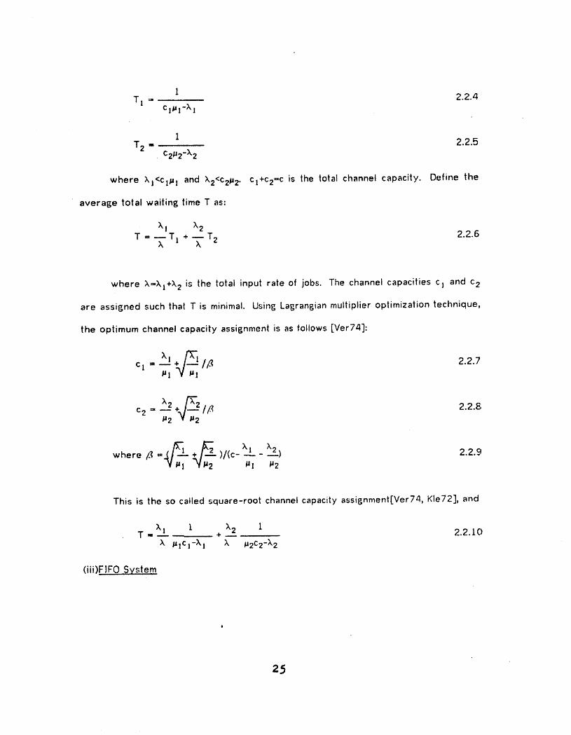
where Xl<cl,u ! and X2<c2p2. Cl+C2=C is the total channel capacity. Define the
average total waiting time T as:
X1 X2
T =--T 1 +--T 2 2.2.6X X,
where X=XI+X 2 is the total input rate of jobs. The channel capacities cI and c 2
are assiF.,ned such that T is minimal. Using La_,rangian multiplier optimization technique,
the optimum channel capacity assignment is as follows [Ver74]:
= _ + !/_ 2.2.7Cl _I
0c2 = _ //_ 2.2.8_12 v _u2
+ 2 XI _where /3 )/(c--,.- X'2) 2.2.9#I #2
This is the so called square-root channel capacity assignment[Vet74, Kie72], and
)'1 1 )'2 1T =__+ 2.2.10X #Ic1-XI X #2C2-X2
(ill)FIFO System
25

C_
FIRGURE2.2.4 F]FO SYSTEM
This system has only one channel wilh capacity c. The jobs come in and are
serviced according to the FIFO (First in First Out) service discipline, regardless of their
classes. The average waiting time is calculated by the formula of the M/G/1 queueing
system [Ver74]:
1 o'Z),_c+ ;k/l_cT = -- + 2.2.11
_c 2(.c->,)
where X.= X1 + X2
= total input rate of the system.
. = X./(X!/_I + X.2/_2) 2.2.12
= the averaBeservicerateofjobs, theinverseofthemean servicetime.
O.2 : [2),.I/(X_,l 2) +2X.2/(_./122)- (_.l/X.#l + X2/X./LI2)2]/C2 2.2.13
= the variance of the service time for the mixed stream.
(iv)Preemptive Priority System
c..
FIRGURE 2.2.5 PREEMPTIVE PRIORITYSYSTEM
The Class I jobs have preemptive priority over Class II jobs. This system is
26

analyzed and solved by Avi-Itzhal,, and Naor [Avi61]. Because of the preemptive
property, the service of Class | jobs is independent of the existence of Class II jobs.
So from the formula of M/M/I queue we will get:
1Tl =, 2.2.14
PlC-Xl
The Class II jobs may be interrupted between service. The average waiting time
is as follows:e
I/_2c * XllI',UlC(.IC-Xl).]
T2 = 2.2.151 - X11(.Ic)- Xzl(.2c)
(v)Non-preemptive Priority.System
C.
FIGURE 2.2.6 NON-PREEMPTIVE PRIORITY SYSTEM
The Class I jobs have priority over Class II jobs in the waiting line. This system.,
is analyzed and solved by Cobham[Cob56]:
I XI/(#IC)2 + X2/(_UzC)2TI = _ + 2.2.16
_=cI i->,i/(_c)
1 X,./(._!c)2 + X2./(#2c)Z
, T2 =_+ 2.2.17#2c {l-;k.i/(#Ic)}{l-X|/(#IC)-;k2/(.2c)}
2.2.3. Comparison
The numerical results are plotted in Figures 2.2.7 and 2.2.8 There are two major
points we would like to mention.
2?

(])The effect of long,iobs. The average waiting time, T, is plotted in Figure 2.2.7,
versus the service request of Class |I jobs. The average service request of Class |
jobs is assumed to be one unit in that figure. Class ] jobs have priority over Class ]I
jobs for priority systems. The average wailing time, T, increases very rapidly' for the
FIFO system and non-preemptive priority system with respect to the ratio Pl/P2" The
reason is that in these systems if a long Class I[ job is serviced, a long queue will be
built up. There is a similar situation in the integrated switch model. ]f the service
capacity for Class [I jobs, c2=c-ic v, is less than x.2/iJ2 and this situation lasts for a long
period, a long queue will be built up. Thus, in the integrated switch model if k2>(c-
iCv),P2 for some i, the average waiting time will increase rapidly with respect to the
ratio P2/Pl, even if X1/Cpl , X2/C_I 2 are kept constant.
(lI)The effect of preemptive and non-preemptive priority. Figure 2.2.7 shows
the total waiting time of jobs versus the length of low priority job service requests.
Figure 2.2.8 shows the total waiting time of jobs with respect to the size of high
priority job service requests. In Figure 2.2.8 the average service request of Class II
jobs is assumed to be one unit, while the Class I jobs still have the priority. The
figure shows that when the longer jobs have priority, there is little difference
between non-preemptive priority and preemptive priority. The interrupted jobs are
the smaller ones, which have little influence on the system behavior. The integrated
switch model implies the preemptive priority of Class I jobs over Class II jobs. This is
not true for the real SENET implementation which uses the non-preemptive priority
scheme. However, the service requests of Class I jobs are several orders of
magnitude higher than those of Class |I jobs in the SENET implementation. From Figure
2.2.8, it is clear that we will expect litlle difference in performance between the real
28

SENET switch and its model. Of course in the integrated switch model, the Class I jobs
will not be queued, and they will not block all of the cllannel capacity c. However,
when the integrated switch is in overloaded state i, where _he service capacity for
Class ][, (c-iCy) , is less than the Class ]l job input rate, ;k2, a temporary queue with
input rate less than its service rate wilt last a long period. This is the reason for the
long queue in Figures 2.2.7 and 2.2.8 and will be the reason for the Ion 8 queue of the
integrated switch.
29

oJl..... 0
• 0
0 I ,.4
jt j
oF-i
.... 1 _ o
Q,° r._o
• G4 _""'° ! _ ffl
"- • O _:t",,. t _ Q
"-., I i_
"-, I 0 O
" M"_ ", [ 6,
El ,_ ,, I r_ _ H4_
® _ \ -, . o+= CQ _ _ 0,,.m _ \ . o
m _ o
0 M _ _
; I I , ,: j', I: I i!
f _
o o o• m •
0 0o 00
AVERAGE WAITING TItlE
30

10000 • 0 ....................
)< , Preemp_iw Priority //
, Non-preem tlve Priority
10.0
eO '
1.o 1o.o lOO.O lOOO.O
JOB SIZE RATIO ''_{_I
FIGURE 2.2.8 WAITING TIME W_LEN LONG JOB HAS PRIORITY
31

2.3. Integrated Switch Model .
In this section, an algorithm is suggested to solve the integrated switch model°
By the memoryless property of the Poisson input processes and the independent
exponentially distrit)uted service requests, the model can be described as a Markov
chain with state (i,j), where i is the number of Class ! jobs and j is the number of Class
][ jobs in the system. The transition rate of the probability ftowin8 out of the state
(i,j) is [Xl+i#l+;k2+di#2] and the transition rate of the probabilities flowing into the
state (i,j) are XI, (i+l)luI, k2, di# 2 from states (i-l,j), (i+t,j), (i,j-1), (i,j+l), respectively,
for O<i<n and j>0. Where.di=c-i,c v is the channel capacity for Class It jobs when
there are i Class ! jobs in the switch. The non-boundary probability transition flow
diagram is as follows:
di#2 _k,,, di#2
FIGURE 2.3.1 TRANSITION FLOW DIAGRAM
In the steady state, the probability transition rate flowing out of a state shouid
be equal to the probability transition rate flowing into tile stale. The steady state
distribution, Pi,j, will satisfy the following balance equations:
32
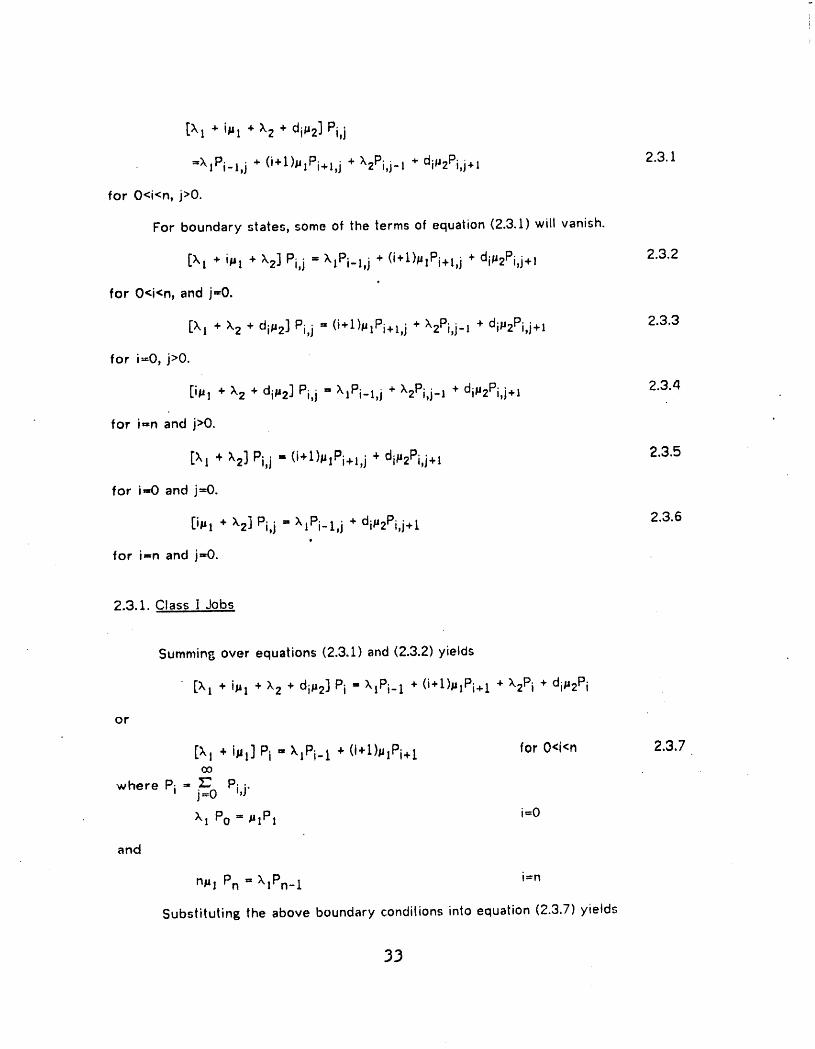
[;k I + i_! + X2 + di_ 2] Pi,j
=XiPi_l, j . (i+l)plPi.l, j + ;k2Pi,j_ ! + diP2Pi,j+l 2.3.1
for O<i<n, j>O.
For boundary states, some of the terms of equation (2.3.1) will vanish.
[)'1 + iPl + X'Z] Pi,j = X'lPi-l,j + (i+l)PlPi+l,j + diP2Pi,J+! 2.3.2e
for O<i<n, and j=O.
[XI + ;'2 + diP2] Pi,j = (i+l)plPi+l,j + X2Pi,j-I + dip2Pi,J +1 2.3.3
for i=O, j>O.
[ip! + ;k2 + di,u2] Pi,j = XIPi-I,j + XzPi,j-I + diP2Pi,j+l 2.3.4
for i==n and j>O.
[;kl . X'2] Pi,j = (i+l)pIPi+l,j + dip2Pi,j+! 2.3.5
for i,=O and j=O.
lip1 + x'2] Pi,j = >'[Pi-l,j + diP2Pi,j+t 2.3.6
for i=n and j=O.
2.3.1. Class I Jobs
Summing over equations (2.3.1) and (2.3.2) yields
[X! + ip 1 + X2 + dip 2] Pi = )"lPi-1 + (i+l)plPi+l + XzPi + diP2Pi
or
[Xl + iPl] Pi = XIPi-1 + (i+l)_lPi+l for O<i<n 2.3.7oo
where Pi = _j=O Pi,j"
;k! Po = PiP1 i=O
and
nPI Pn = ;klPn-I i=n
Substituting the above boundary condilions into equation (2.3.7) yields
35

X.IPi = (i+t).ulPi+ 1 for O<i<n 2.3.8n
'b
Top=ether with the condition that Pi s are probability functions, i.e., i=_oPi=t, Pi
can be solved as:
i i (i' i).Pi = %" :kl ' _;
andn 0
Po= [ i_Ox1_/ (i! _I_)]-l.
GI, lhe grade of service for Class l, will be'
GI - blocking probability for Class I jobs.
= a new Class I job comes in and finds the system at slates (n,j).
= probability thal system has n Class I jobs.
= Pnn
= ;kln/(n!pln) / x'lj/(j ! _lj)] 2.3.9
This equation is known as Erlan_ B loss formula [Sys60]. The 8rade of service
for Class I jobs is the same as the grade of service for an M/M/n/n queuein6 system
for line-switching. The Class ] jobs have inherent preemptive priority over Class ]I
jobs, so the system state of the inteBrated switch for Class I jobs is the same as in a
system without any Class II jobs. Figures 2.3.2 and 2.3.3 show the numerical behavior
of equation (2.3.9). The channel utilization factor u is defined asn
u='_ ii=O n" Pi 2.3.10
2.3.2. Class [[ Jobs
For Class ][ jobs, the variation of the queue length is much more complicated.
Define:oo oo
hi(z) = _' 2.3.1 tj=O zJPi,J / j_F"=OPi,j
= generating function of Prob[ Number of Class I! jobs ]i Class ! jobs]
34

p- _,I_
GRAD p -15.0E
O, F p -10.0
S .1E .0 p -5.0
, R; V
IC!
E
iI
i! .Oi' 0 1 2 4 6 8 " 10 12 14 16 18 20I
't NUMBEROF REAL.TIk4ECHANNELS •
FIGURE 2.3.2 GOS OF CLASS I JOBS
f
35
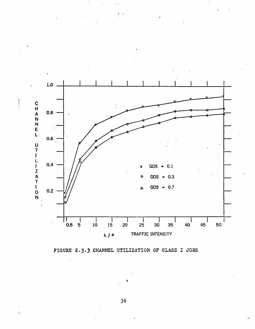
1.o I , ! ! [ i ! I ! I
CHA 0.8NN
EL
0.6UTILl 0.4 x COS = 0.1ZA o. GOS = 0.3TI a GOS = 0.7O 0.2N
FIGURE 2.3.3 CHANNEL UTILIZATION OF CLASS I JOBS
36
!

= conditional generating function for Class II jobs with i Class ! jobs.
Multiplying equation (2.3.1) by zJ and summing over all j, we have:
[;k I + ip I + X.2 + diP;,] ni(z)' Pi
I=x I ni- l (z)Pi- ! +(i+1)p I ni +l (z)Pi + 1+k2z rti (z)Pi +dip2/z" ni (z)Pi-di P2( ] -_" )Pi,o
Substitutin8 equation (2.3.B) into the above equation yields :
[X t+ipl +;k2(1-z)+diP2(1-1/z)]ni(z) -iplni_l(z) - ),lni+l(Z)
1= dii=2(1-_')Pi,0 / Pi" 2.3.12
for 0<i<n.
Similar methods yield:
[;kI *;k2( IL-z)*di,2( 1-1/z)]ni(z) - x _ni. 1(z) = dil,2( 1-1 )Piio/P i.2.3.1 3
for i=0,
[i_ ! +;k2(1-z)+diJu2( 1- 1/z)]ni(z) - i_4lni. 1(z) = di#2( 1_l)Pi,0/Pi 2.3.14
for i.-n.
To simplify the equations, define
ui(z) = coefficient of hi(Z) of equation (2.3.12)
1= ;',! + ip! + X,2(I-z) + dip2(1-_-) 0<i<n 2.3.15
and
Un(Z) = np ! + k2(I-z) + dn#2(fL -1-)Z
Similarly
b i = coefficient of the riEht hand side of equation (2.3.]2)
= di,u2 Pi,o'/ Pi 2.3.16
Equation (2.3.J3) and (2.3.14) can be rewritten in the matrix form as:
tA(z) n(z) = (1-_-) b 2.3.J7
where n(z) and b are column vectors with ith element hi(Z) and bi, respectively.
n(z)=[no(z) n l(z) ......nn(Z)] T
37

b =[b o b I ......bn ]T
of dimension (n+l), where T stands for the transpose of a vector.
A(z) is a square matrix as follows:
Uo(Z) -X1
-_l ul(z) -xl (_
A(z) =
. -i_41 uL(z) -X1
. . -kl-n .1 un(z)
We will solve the hi(z), or Prob[ j lii from equation (2.3.17). First b is solved
from the following two properties of rti(z)"
(i) hi(l) - 1, for all i, because hi(z)is a p=enerating function of a probability
distribution. From equation (2.3.1 1)oo (30
hi(l) = '_ jL-'__0 =j=O Pi,j / Pi,j 1.
(ii) hi(z) are finite in the re_;ion O_<z<l for all i.
Oo 03
hi(z) .. 'C /j=O zJPi,J j_--O Pi,j
03 03
<Z::; /- j=O Pi,j j_L-'_OPi,j
= 1 for O_<z<l
This implies that if hi(z) can be expressed as ni(z) = f(z.._.).)then for all zj such6(z)'
that zj in (0,1) and g(zj)=O f(zj)=O.
From the two conditions above, b can be determined. The algorithm is given
below. First define a matrix R(z) with (i,j) element rij(z) such that:
38

rij(z) = (-t) i+j * a.*.l_(z).
where a.*.(z) is the cofactor of aji(z), the (j,i)th element of matrix A(z).J!
By the theory of matrices [Wyl60],I'1 n
j=Ots the determinant of A(z) with ith column substituted by the kth column. If i#k, then
this determinant has two identical columns, i and k, and the value of tl_e determinant is
zero. If i=l,,, the value is the determinant of matrix A(z). We have:n
j=O_ rij(z)" ajk(z) = 8ik IA(z)l for all i,k 2.3.18
Following a similar argument, it can be proven that:n
aij(z) • rjk(Z) = Bik IA(z)l for all i,k 2.3.19j=O
where 6ik is the Kronecker delta, such that
0 i#k_ik = {
l i=k
H43nce
R(z)A-t(z) =
where IA(z)l is the determinant of matrix A(z). So equation (2.3.17) becomes
R(z) 1rKz) = _ (1-_) b 2.3.20
f(z)In other words, n(z), expressed in another form, is _ of a generating function.
All zeros of the denominator in the region (0,1) must also be zeros of the numerator.
Theorem 1_:IA(z)l=determinant of A(z) has exactly n different single roots in (0,1), and
z=l is also a root.
This theorem can be proven by using methods similar to those of [Mit68]. The
basic argument follows: IA(t)I=0 is trivial, for the row summation of A is zero.
]9

Define F_i(z) as the principal minor of order i of A(z). Then IA(z)l is equal to p=,n(Z),
a polynomial of degree (2n+2).
I Uo(Z) -xj 0 0 0 0 II -_I ut(z) -x_ 0 0 0 I
gi(z) - I o o II 0 0 ' ' " ui-_(z) ">'1 II 0 0 0 . -i_ ui(z) I
Clearly',
gi(z) = ui(z)gi_l(z) -iXl_Igi_2(z) for i>l. 2.3.21
with go(Z)--Uo(Z), and g_1(z)=1.
By ui(O)-*-oo , ui(oo)-.,-oo, and ui(l)--X.l+i_j>O. It is easy to see that the signs of
gi(O) and gi(oo) are (-1) t+t, and _i(1)>0 for all i<n.
From the above property, it is clear that there is one real root zl(O) of go(Z) in
(0,1), and one root in (1,oo), because 6o(0)<0, go(Oo)<O,and p=o(1)>O. Substitutinl_
zl(°) into equation (2.3.21) yields
_l(Zl(0))= Ul(zI(O))_,I(Zl (0)) - ;kl_ 1
= -_,x_x<O
and
gl(O) <0, 81(I) > O.
So there is one real root of _l(Z)in each of the regions (O,zl(°)) and (zl(°),I),
and lhere are two tools in lhe region (i,oo). By lhe same technique, cotm|tn_,
the number of sil_n changes in the sequence 6i(z), one can determine the number
of zeros of gi(z) in (0,1). If zj (i) is the jth root of 8i(z), then the consecutive
_,j+t(zj (i)) will have different signs. Thus zj (i+1), roots of 6i+l(Z), will be in
(Zj_l(i),zj(i)) interval for j=0,1,..,i. The proof can be continued by |he above
interval partition procedure iterativety from i=1 to n. The number of roots of
/4,0

gi(z) in (0,1) will be equal to (i+1) for all i<n. When i=n, one is also a root, the
interval (Zn_l(n),t) does not have a root, and the total number of roots for IA(z)i
in (0,1) is n. The same procedure is also carried out numerically to find all the
roots. #
Theorem 2_:R(z i) has rank one for all z i of a root IA(z)lin (0,1].
Suppose that rj is the.jth row of matrix R(z) and that ak is the kth column of
A(z). Then from equations (2.3.18) and (2.3.19),
rj. ak ,= bjk IA(z)l for all i,k. 2.3.22
Now for O<z<l and tA(z)l=0,we will have
r i • ak = 0 for all i,k. 2.3.23
IA(z)l only has a sinsle root in (0,1), because there are n independent ak out of
(n+l) column of A(z). For any row vector x of dimension (n+l), if there exist n
independent row vector ak such that x. ak=0, then x has only one degree of
freedom. For any ,} such that }.;k=0 for l<_k<_.n,it is implied that _=¢_;, for a
scalar _. This is equivalent to saying that in a space of dimension (n+l) with n
independent linear constraints, the solution will always be on a straight line, i.e.,
y=o_.X. #
Because R(z) has a rank equal one for all 0<_zi<_.land IA(zi)[,-O, any row of R(z)
can be chosen as r(z i) and satisfies the followin{_ equations:
r(z i) - b = 0 for O<_zi<Z, i=t,2,.., n 2.3.24
and
r(Z)" b = _ IA(z)lz_ 1 2.3.25
Now that we have (n+l) unknown and in+l)independent equations, b i can be
solved.
41

The element of r(z i) is the determinant of an n dimension submatrix of A(zi).
Since R(z i) has rank of one, any row of R(z) can be used. If the zeroth row is chosen,
the result is:
I u;+l(z) ->'1 0 0 I] -tJ+2),l uj+2(z) -XI 0 I
rj(z) = x.IJ. ] ......... 0 ]I 0 0 • • • Un_l(z) -;E1 II 0 0 .... n,_1 Un(Z) I
Basically all rj(z) follow the three term iteration:
uj+l(z) (J+2)# 1
rj(z) - x't rj+t(z) - ------Xt rj+2(z) 2.3.26
Because there is one degree of freedom for all ziP0, we can set any ri(z)=l and
calculate the rest of rj(z).
R(1) has a very special property' Not only is every row linearly dependent on
each other, but every row is exactly the same. Thus for any row, the jth element of
the row vector is as follows;
rj(1) ---(n! ,uln) • x.lJ / ( jr pl j) 2.3.27
because uj(1)=Xl+j#l, and the summation of all row, except one, is zero.
In order to calculate equation (2.3.25), we must first calculate d--_lA(z)l. The
derivative of a determinant is the summation of determinants, each with a derivative on
one row of the original matrix. Son
d-_'IA(z)l= i--'_OjAi'(1)l 2.3.28!
where Ai (z) has elements that are the same as those of A(z), except for the ith row,
which is the derivative of the ith row of A(z).
By a straightforward manipulation, it can be proved that:
n)]Ai(z)lz=l =(n!#l • >,1_ /(i _#}_). ui(1) 2.3.29t
where ui (z) is the derivative of ui(z) with respect to z.
42

n
diA(z)lz=l = i=Z:;0(n! _ln) - X_i / ( i !.=i) • (-x2 * dpu2) 2.3.30
Substituting the ri(1) into the above equation, we have:n n
rj(1) bj = ',_ rj(1) • (-X 2 + dj_ 2) 2.3.31j=o j=o
r j(1) is proportional to Pj, the probability of the system having j Class I jobs.
Let r j(1) be normalized and be equal to Pj. There is a physical interpretation of the
above equation, bj/(djiu2)=Pj,o/Pj=Pol j is the probability that no Class II job is in the
switch when there are j Class [ jobs in the system. The left hand side of the equation,
which is tt_e summation of the probability that the channel has no Class I[ jobs
multiplied by the service ability available, is equal to the whole wasted channel
capacity. The second term of the right-hand side of equation (2.3.3t) is the total
service ability for Class ]I jobs. Thus the right hand side , which is the service abililty
available minus the service requests, is also the total wasted channel capacity.
By the n homogeneous equations of (2.3.24) and the above non-homogeneous
equation (2.3.31), bj can be solved uniquely. All other system parameters can be!
derived from bj. We next give an example of how to calculate n i (1), the average
queue length when there are i Class ] jobs in the switch.
1If we differentiate equation (2.3.J7), A(z)n(z)--(l-_.)b, with respect to z, we get:
A'(z)n(z) + A(z)n'(z) = b/z 2 2.3.3;!
or
A(t)n'(t) = b - A'(Z)-1
where 1 is a vector with all the elements containing one. The ith row of the vector
equation is:
Xl[ni'(1 ) _ ni+l'(1)] + i_l[rti'(1 ) - ni_l'(l)] = b i + X2 - dip 2 2.3.33
for O<i<n.
Xl[no'(1)- n='(1)] = bo +x z-do_ z
43

and
npl[nn'(1 ) - nn_l'(1)] = bn +k2 - dnp 2
With bi's known, there are (n+l) variables, r_'([), but the (n+l) equations above
are not linearly Independent, for the determinant IA(1)l is zero. An extra equation is
' R(z)needed to solve the n (1). Multiplying both side of equation (2.3.32) by A-l(z), [-_-_-,
we get
' 'n (z) = [b/z 2 - A (z)n(z)] 2.3.34
If we let z approach 1 and use the L'Flospital's Rule to calculate the resulting
limit, we get=
n'(1) = {R'(z)[b/z 2- A'(z)n(z)]
+ R(z)[-2b/z 3 - A"(z)n(z) - A'(z)n'(z)]} / [dlA(z)l] z=l
= {R'(t)[b - A'(t)n(1)] + R(I)[-2b - A"(l)n(1)- A'(1)n'(1)]}/a 1 2.3.35n
= d-_ = _ rj(1)(-X2+djP2) ,where a! IA(z)lz=l j=0
A'(1) and A"(1) are diagonal matrices with elements (-X2+dit_2) and (-2diP2),
respectively. Because all rows of R(1) are the same, ni'(l) can be written in the
following form:n
! I
ni (1) = {j_L"_ORij (t)[bj - X2 + djl,2]
ni
+:_ rj(1)[-2bj - (-X 2 + 2.3.36j=O - 2diP2 djP2)nj ([)]} / al
Because only one equation is needed from the above to solve n'(1), let i equal
zero. Then:n
' - _0 '(rt0 (1) = _0 + [a2 ,,fjr[j t)]/a 1 2.3.37
wheren t
_0 = j=O_ R°j(1)[bJ + x,2-djp2] / al
l'j = rj(1)[-k 2 + dip 2] = n! pl n. klJ(-x, 2 + djp 2) / (j ! #lJ)
44

n n
al ,= jL"=O"rj = j-O;E;rj(])[-;k 2 + dj_2]
n
= n!/Jl n j_=OXIj" (-;k2 + dj/_2) / (j !/Jlj)
n
a2 = j_=Orj(t)[-2bj + 2dj#2]
where Ro,j'(I) of equation (2.3.36) is 8iven by the derivative of equation (2.3.26).
Ro,n(Z) = ;kin implies Ro,n'(1) = O.
Ro,n_l(z) = ;kl n-I Un(Z) implies %,n_l'(1) = ;kl n-I Un'(1)
and by equation (2.3.26):
uj+t(z) (j+2)/_ Ir j(z) ,= r j+ l(Z) rj +2(z)
>'1 ;kl
uj+ l'(Z) u;,. l(z) (j+2)u 1
R°'J'(Z) " ;kl R°'j+l(Z) - _'*;k_ R°'j+t'(z) - ;kt R°'j+2(z)
t
and
-Xo+d_,,> ;kl+(i+l)., (i+2)_,1Ro,j'(1)= '- J'- " "" ' " "
;kt rj+t(1) - ;kt Re,j+ 1 (1) >'1 rj+2(1) 2.3.38
With equations (2.3.36) and (2.3.37), ni'(t) can be solved by the (n+t) linearly'
independent simultaneous equations. Numerical results are shown in the Tables 2.1,
2.2 and 2.3 and are plotted as curves of exact solution in Figures 2.6.J._ 2.6.2, and 2.6.3
of Section 2.& rq'(1) increases rapidly with respect to i, the number of Class I jobs in
the switch, rti'(t) is also a function of /J2h'], the ratio of Class | service requests to
that of Class II jobs. fti'(1) increases very rapidly with respect to /_2/_ 1, even with
fixed traffic intensity of Class ] jobs and Class ]I jobs, i.e., Xl/tJ I and ;k2//l 2 remain
unchanged. The difficulty in calculating numeric results from the above algorithm will
be discussed in Section 2.4, and the numerical results will be discussed in Section 2.6.

2.3.3. Multi-Server Model
If the number of servers is more than one, and a job can only be serviced by at
most one server simultaneously, then some modifications have to be made for tile
above ai6orifhm. Let us use the following notation=
• p - number of _ervers in the switch.
Cp = channel capacity, or service ability of each server.
then c = p * Cp.
di(j) = channel capacity for Class II jobs when the system is in stale (i,j)
= mint(c-iCy), jCp}
For all j > (c-iCv)/Cp, di(j) equals (c-iCy) , the channel capacity left for Class |[
jobs when the system has i Class I jobs. E3y a straightforward manipulation, an
expression similar to equation (2.3.17) can be written:
A(z)n(z) = (1-1)b(z) 2.3.39
Instead of being constant, b(z)is now a function of z with jib element bj(z)"
bj(z) = E:_ (di-jCp)#2zJPi,j / Pi 2.3.40O<j<(p-i//_)
where 13=Cp/Cv, and
b(z) = the(z) bl(z) bz(z) ..... bn(z)] T
Follow{ng exactly the same procedure, we derive n homogeneous equations
similar to equations (2.3.24).
r(z i) • b(z i} = 0 for 0<zi<I ,i=1,2,3,...,n.
for all roots z i of IA(z)l in the range (0,1), and one non-homo£_,eneous equation similar
to equation (2.3.25):
= d-_IA(z)lz=lr(1). b(1)
All of Pij' such that O<j<(c-iCv)/Cp, are unknown variables in b(z), and the
46

number of variables exceeds the number of equations. Now some of the equations of
(2.3.1) which are not used in finding equation (2.3.39) can be used as supplementary
equations. These equations are:
[X! + ipl + X2]Pi,o = X.lPi_l, o + (i+l)plPi+|, o + diP2Pi, 1 2.3.41
for all (c-iCv)/Cp>l. And
[;kI + ip! + X,2 + dip2]Pij
= XIPi_], j + (i+l)plPi+l, j + x,2Pi,j_} + diP2Pi,j+ l 2.3.42
for all ] < j+l < (c-iCv)/C p.
For each Pij, j>O, in b(z), there will be a corresponding equation in either of
equation (2.3.41) or equation (2.3.42), so the total number of equations will always
equal the number of unknowns. For a special case, Cv,-Cp, the problem is the same as
[Bha75], and the number of simultaneous equations becomes p(p+l)/2. All Pij, with
O _<.I < (c-icv)/Cp, can then be solved by these equations. With all Pi,j, O-<J<(c-iCv)/Cp'
b(z) can be calculated from equation (2.3.40). Following; the procedure of the uni-
server example of the last section, all syslem parameters can then be derived.
Next comes the example to solve hi'(1) for the general multi-server case.
The corresponding equation (2.3.32) becomes:
e i 1 t
A (z)n(z)+ A(z)n(z)= b(z)/z2 + (1-_-)b(z) 2.3.43
or
A(1)n:'(1)= b(1)- A'(1)"I
These are the same n equations(2.3.33)as |hose for the uni-server case. The
extra non-homogeneous equation is derived in a manner similarto that of the uni-
server case.
n'(z)= ]-_R(z)[b(z)/z2+ (1-_-)b(z)- A (z)n(z)] 2.3.4q
Let z approach to one and use the L'Hospitat's Rule to calculate lhe limit.
_7

n'( t )=t/[dlA(z)lz =1]"{R'(z )[b(z)/z 2 +(t-_b'(z)-A'(z)n(Z)]z
I 2 ii ! t
+R(z)-[-2b(z)/z3+2b (z)/z -A (z)n(z)-A(z)n(z)]Iz_ t 2.3.45e
Choose the first row, i=O, as the extra equation needed to solve n(]) of
equation (2.3.43). The same form of equation (2.3.37)is derived:ne i
n o (1) = 4_o . [a2 - j_--O_,jrtj (1)]/a 1 2.3.46
with minor modification of a2, where 4'o, _j and a 1 have the same definition.f
n !
a_ - j_--Orj(1)[-2b](i) + 2bj (1) . 2dj_2]with
n
= '(_o j=_O R°J 1)[bj(1) + X2 - dj_2] / a I
\ "rj = rj(1)[-X 2 + dj. 2] = n! #l n (-;k2 + dj_ 2) /(j !_I j)
n n
a! = j=O:E"rj = j=OZ:_rj(1)[-;k 2 + dj.2]
n
"= n! ;41 XlJ" (-X2 + dj"2) / (J _ #1j)
'(ROj 1) are exactly the same as the uni-server case.!
With equations (2.3.45) and (2.3.46), hi(l) can be solved by the (n.t) simultaneous
equations. Numerical results are shown in Table 2.1 and plotted in Figure 2.6.1 of
Section 2.6. In bolh the uni-server and the multi-server systems, we can see little
!
little variation in n i (1) in over loaded states. This is a similar situation with that of
average queue length of an M/M/p queue and of an M/M/1 queue with the same traffic
intensity varies much less in heavy traffic than in the light traffic.
The conditional average queue length, hi'(1), increases rapidly with respect to i
for both uni-server and multi-server. The rale of increase depends on the ratio of job
!
requests, _2/_1. For large _2/_1 , rti(1) in overloaded states may be several orders of
1,8

t
magnilude higher than hi(I)in underloaded states. Although the probability that the
system will be in the overloaded states is small, the long queue length built up in these
states contributes much to the total average waiting length. The long queue length in
overloaded states also causes many other problems, such as the problem of buffer
space for Class ]] jobs, flow control problems, and congestion problems.
]n underloaded states differences between multi-server and uni-server will not
affect the overall performance of the integrated switch as much as they will in
overloaded states. For the above arguments, a multi-server integrated switch has
approximately the same performance as a uni-server switch with the same total
service ability.
49

2.4. Error Analysis and Condilional Mean Approximation
As it is mentioned in Section 2.1 (XI, #]) and (X2, 142)differ from each other by
several orders, of magnitude. To deal wilh numbers which are combinations of very
large numbers and very small numbers, a relatively Ion_, computer word size should be
used to retain the information. For example, if a=100, and b=0.01, then a.b=J00.01
needs five dip=its of precision, and (a+b)2-a2-2,ab = 10002.0001-10000-2 = 0.0001
needs as many as nine diE,its of precision to get the risht result. A much greater need
for precision arises in the alBorithm of Section 2.3, in which there is high order
multiplication of the form (a+b). Thus in solving; the integrated switch model, the
rounding error does restrict the maximum dimension which can be solved by a specific
computer word size.
2.4.1. Error Analysis
Let us first review the whole al_,orithm. There are four steps: Find the roots of
IA(z)i; calculate rj(z i) which is the cofactor of aj,o(Zi); invert the matrix R(z i) to solve hi;
finally, calculate the required parameters from bis. The first step is basically
calculating the determinant of a band matrix, or calculatin_ a three-term recurrence
formula. Define Ai the ith principle minor of matrix A, that is:
J all a12 0 ''' 0 II a21 a22 a23 •.- 0 J
Ai = J 0 a32 a33 "'" ai_li IJ 0 0 " " ' aii- I aii l
or
Ai = aii Ai_ I - aii= I . ai_li Ai_ 2 i>2 2.4.l
where A 1 ,, ali , and Ao = 1.
. 50

In general the three-term recurrence formula is not numerically stable. The
above equation can be simplified to equation (2,3.26) as follows'
uj(z) (j+l)# 1rj_l(z) = _ rj(z) - ------.- rj+1(z) 2.3.26
;`1 ;`1
where uj(z) = ;`1 . J#! . ;`2(l-z) + (c-j*Cv)pz(1-1/z)"
To study the numerical stability of the above equation, let us suppose that there
is a rounding error, dr j, of rj(z), then the rounding error of rj. 1 will beQ
o
drj_! = [uj(z)/;`t]. drj + [uj (z)/;`l] • rj(z) dz 2.4.2
In general, uj(z) and uj (z) will not be zero for zi a root of IA(z)l=O,and thet
error of drj, dz i will be exagBerated by factors uj(zi)/X 1 and uj (zi), respectively. For
a problem with XZ/;`I=103, for each recurrence, the rounding error will increase by'
the same order, or 10 bits of precision will be lost. A PDP-10 double precision word
has 72 bits, and it can only solve a problem in the order of X2/XI=103 and n=7.
The above is a very rough error analysis. Consider the example:
Let X1 = 1, =u]= 1, c = 1.2, cv = 1, k2 = 5000, #2 = 10000.
Then
Uo(Z) = ;'I+ X2(1-z)+ c_2(I--I/z)= -5000z + 17001 - 12000/z.
u1(z)= #I + )'2(l-z)+ (C-Cv)P2(1"I/z)= -5000z + 7001 -2000/z.
IA(z)l=,Uo(Z)• ul(z) - ;`l_l
= 107,[2.5z 2 - 12.001z + 18.9024 - 11.8014/z + 2.4/z 2]
= 107,(1-1/z)[2.5z 2 - 9.501z + 9.4014- 2.4/z]
It is easy to see that only one root, z], of IA(z)l is in (0,1). The corresponding
equation is as follow:
ul(zl)b o . ;`tbl = 0
with z= 1

ul(1)b 0 + >`lb 1 = IA(z)l(1-l/z) Iz=l = 4000
This implies
b0 = 4000 / [1-Ul(Zl) ] and b I = =boUl(Z 1)
Now we have:
•o = ,ul[-X2+ c#2] = 7000
I = -X2 + (C-Cv)U2= -3000
a l = _'0 + ?! " 4000$
a2 = [-2b o + 2c# 2 - 2bl + 2(C-Cv)/_2] = 2.104i i w
ROI (I) = 0, and Roo(1) = ul (1)=-3000.
3@o = -3000[bo + >'2- c/a2]/al = 1_[b0 - 7000]
i I
The two equation of rlo (1) and rl I (1) are
I I( m%(1)-nl l)=b o 7000
I I
11no (i) - 3r(j(I) = 20 - 3[bo - 7000] 2.4.3
They can be solved as:
' 3no(1) = 2.5-_-(bo- 7000)
' 4
n_(i)= 2.5-7(bo-7000) 2.4.4I I
With the above formula,rlO(I) and ril(i)are solvedwithout any rounding error°
i
Ifthere isa rounding error of zl,then the roundingerrorof rlo (I)willbe:
dri 0(1) = - db 0
= -3000 / [1-ul(zi)] 2- dul(z l)
= -3000 / [1-ul(zl)] 2. ul'(z 1) dz 1
~ -3000,7506.45 dzl
~ 2.25,106 dz I 2._1.5
where z1=0.399866733 , Ul(Zl)=-6,10-5 and ul'(zl)=7506.45
52

A rounding error of dz! is exag,gerated by a factor of 2 million, i.e., 20 bits of!
precision are lost to rlO(1).
The above example also shows that the numerical instability comes from the
problem rather than the algorithm. Whatever the alBorithm is, the final representative
must be the same as equation (2.4.5). Hence, we should use as many bits of precision
as are available to calculate the all]orithm. Because of the difficulty of calculating the
exact solution, a simple conditional mean approximation is suggested in Section 2.4.2,
and a more complex diffusion approximalion is derived in Section 2.5. The
approximation will have less precision, but it can be useful when the calculation of the
exact solution is not feasible.
2.4.2. Conditional Mean Approximation
Here we Bive a simple approximation alBorilhm for a uni-server intel,,,rated
switch, rii(z) is defined as equation (2.3.11), the generating function of the number ofi
Class I! jobs in the switch, given that there are i Class ! jobs in the switch, r_i(1),
which is. the average number of Class !! jobs in the switch, _,iven that there are i Class
! jobs in the switch, is called the conditional moan. ]n the followin_ approximation, only
ii
the parameters hi(l) are estimated. Let us state the basic system equation (2.3.J2) as
follows:
[;kl+ip_+X2(1-z).dil=2(1-1/z)]ni(z ) -i,u]ni_l(z) - X.lrii+l(Z)
1= di,2( 1-_.)Pi,o / Pi" 2.3. i 2
Differentiating the above equation with respect to z and lettin8 z equal i, we
will getq ii !
(-X2+di,_=2)ni(1)+(X.l+i_l)ri i (1)-i_=jni_ l (1)-Xlni+ ! (1)=diP2Pi,o/Pi 2.4.6
.53

hi(I) equals i, because hi(z) is a generating function of a distribulion. The
above equation can be simplified as:
! I !
• -(Xl+i_l)lt i (t)+i_lni_ 1 (1)+X]ni+ 1(1).--->`2+di_2(1-Pi,o/P i) 2.4.7I
In Section 2.3, we tried to solve Pi,o/Pi and hi(l). However, in this
approximation we only estimate the relationship between them. in an ordinary M/M/1
queue, the average queue lenglh w=p/(1-p)=(1-Po)/P O, or in another form
PO = 1/(1 +w) 2.4.8
Assuming that this relation is a good approximation for the integrated switch, or!
Pi,o/Pi = 1/(1 +n i (1))
we will get the following equation:
! I( | i-(Xl+i_ui)n i (1)+i_lni_ l 1)+Xini+ 1 (1)=->`2+dil,2[1-1/(l+ni (1))] 2.4.9!
for i=O, 1, 2, -, -, n. There are (n+l) equations and (n+l) variables, hi(l) can be
solved. Since, these (n+l)equations are nonlinear, an iterative method is used to solve
si(m)them. Let be the rnth iterative value of n i(1); equation (2.4.9) can be rewritlen
(m)+x i (m) = ->'2 2.4.10-[k I +io 1+di_2/(l +gi(m- l))]_i(m)+i_ ]gi- l $i+I
With a reasonable initial guess of gi[(O)], we can solve the (n+l)-simultaneous
equations and get 8i (I) and so on, i.e., _;i(2), .,., gi[(m)]. This iterative method
converges quite rapidly. Figures 2.6.1 and 2.6.2 compare the approximation results
and the exact solution.
I
This approximation shows rapid increasin$ of n i (I) with respect to .u2/ji I as well
as rapid increasing of i, as in the Kummerle's approximation, but it is much smoother
and closer to the exact solution. The Bhal's al[,,orithm and approximation are based on
the multi-server system. As shown in Figure 2.6.4 of Section 2.6, the solution of
54

Bhat's algorithm matches other methods, but its approximation fails to show the
increasing of the mean waiting length with respect to _2/,u]. Unfortunately, P2/_] in
the order of thousands is the practical situation and the most important case, and the
approximation differs many orders of magnitude from the exact solution.
55

2.5. Diffu(.;ion Approximation
If the service ability for Class l[ job is always greater than the input rate,
c21A2=(c-i_Cv)_2>X2 , then the system will almost always have a shot! waiting line. If, on
the other hand, there is some i such that (c-i:_Cv)#2<X.2, then there will be some periods
during which there will be a Ions; queue. During time periods when input rate is
greater than the service rate, a queue will be built up. The way the queue 8;rows is a
time-dependent queueing problem. It is welt-known that a heavily loaded queuein8
system can be approximated by diffusion process [Gay68] for both asymptotic and
time-dependent cases. First we will show that the solution of the queueing system in
Section 2.3 is equivalent to the solution of a set of a time-dependent M/M/1 queuein8;
system, then we will use diffusion process to approximate the overloaded states.
2.5.1. Time-Dependent Syster0
Let an M/M/1 queueing system with Poisson input rate X and exponentially
distributed service time of mean 1/_ start at time zero with initial condition h, where h
is a row vector with ith element, h i, the probability that there are i customers in the
system. Suppose that the queue is finite and that _'hi=l. Distribution of the number
of customers in the system at time t, p(t), satisfies the Kolmogorov forward
equations[Kar66].
p'(t) = p(t) A 2.5.1
p(O) = h.
where p(t) is a row vector With j th element, the probability that there are j customers
in the system at time t, and A is the infinitesimal _,enerator of the system with element
aij=O except for i-l<j<i+l:
56

ai,i- l = _u,
ai,i+ ! = X,
at,i = -(at,i_ 1 + at,i+ 1)
-ao, 0 - a091 = X./
-X X 0 0
0 2 _ -(2 _q-x) x
0 0 3_ -(3_x) x . .A=
it_ -(it +X) X .
p(t) can be solved as:
p(t) = h eAt 2.5.2
If the period t ends randomly with exponential distribution of mean l/s, then the
distribution of number of customers in the system when the period ends is:
foo e_St foop*(s) = 0 p(t) s dt =s 0 he At e -st dt
=s h [sl - A! -1
= h [l - A/s! -I 2.5.3
where !is the unit matrix.
Because Of the extremely long holding time of Class } jobs in integrated switch,
the service of Class II jobs can be modeled as one M/M/1 queue followed by another
with different service rate. The service rate for Class ]I jobs is di=(c-icv), wtlich
depends on i, the number of Class ! jobs• We will model the integrated switch during
• 5?
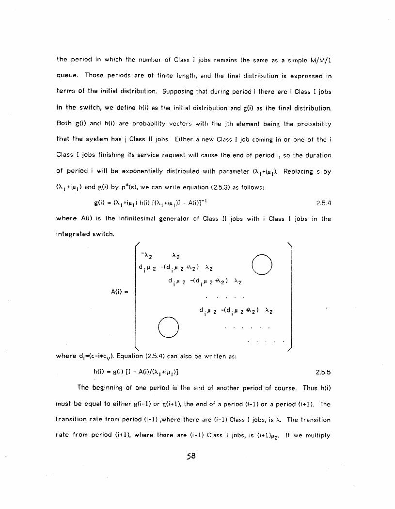
the period in which the number of Class ] jobs remains the same as a simple M/M/1
queue. Those periods are of finite length, and the final distribution is expressed in
terms of the initial distribution. Supposing that during period i there are i Class ] jobs
in the switch, we define h(ii as the initial distribution and g(i) as the final distribution.
Both g(i) and h(i) are probability vectors with the jth element being the probability
that the system has j Class I[ jobs. Either a new Class I job coming in or one of the i
Class I jobs finishing its service request will cause the end of period i, so the duration
of per]oct i will be exponentially distributed with parameter (,kl+i_l). Replacing s by
(X.l+i#l) and g(i) by p*(s), we can write equation (2.5.3) as follows:
g(i) = (X.l+i#]) h(i) [(X.l+i_])] - A(i)_]-1 2.5.4
where A{i) is the infinitesimal generator of Class [I jobs with i Class I jobs in the
integrated switch.
-X 2 X2dip 2 -(di_' 2"&.2) x.2
d._ 2 -(d /J 2 +k2) X2, iA(i) =
dis 2 -(di_ 2+'k2) )'2
@ . ./
where di=(c-i,Cv). Equation (2.5.4) can also be written as:
h(i) = 6(i) [l - A(i)/(X l+i_l) ] 2.5,5
The beginninp., of one period is the end of another period of course. Thus h(i)
must be equal to either g(i-1) or g(i+t), the end of a period (i-t) or a period (i+].). The
transition rate from period (i-t),where there are (i-l)Class ] jobs, is X. The transition
rate from period (i+[), where there are (i+t) Class i jobs, is (i+1)#2. If we multiply
58

these transition rates by their steady state probabilities, PI-| and PI+! respectively,
we get the following ratio of absolute transition rate:
XIPi_ I (i+ 1)._I Pi-.,Ih(i) = g(i-1) + _(i+1) 2.5.6
klPi_1+(i+l)_lPi+l - _,lPi_ I +(i+l)plPi+l
where Pi is the steady state probability that the system has i Class ! jobs. Then
ip I X1h(i) = g(i-1) + _ g(i+l) 2.5.7
ipl+X 1 i#l+X I
Substituting equation (2.5.7-) in equation (2.5.4) yields
g(i) [I-A(i)/(i_l+Xl)] - [ila I g(i-1) + ;_l g(i+I)]/(i_l+;ki) 2.5.8
The jth element of the above row vector is
gj(i) - [gj_l(i)X 2 + c2(i+l)#2gj+l(i)- (X.2+c2(i)o2)gj(i)] / (x.l+ipl)
= (iPlgj(i_1) + ;klgj(i+l) ) / (i_l+Xl) 2.5.9
or
[X.z + ipl + X2 + c2(i)p2 ] gj(i)
= X.lgj(i+l) + i/_igj(i_l) + >,2gj_l(i) + c2(i)_u2gj+l(i ) 2.5.10
where c2(i) = c - i*c v.
This is exactly the same balance equation set (2.3.1) of Section 2.3, with Pij/P i
as gj(i). Thus the integrated swilch model is exactly a set of time-dependent simple
queueing systems. Notice that gj(i)is the distribution of Class II jobs when the system
leaves period i, while Pij/Pi, defined in Section 2.3, is the steady State distribution of
Class II jobs when the system is in i Class I state. The reason that they are the same
can be explained by the "Waiting Time Paradox". This paradox arises from random
sampling of Poisson process:
(t l, t2, t3, ....... , tm) are the times when the events of the Poisson process
happen, and s is a random sample point. Suppose that s falls in (ti_l,ti).
59

S
I i I i I I t I tl 1 i It 1 t 2 t 3 t 4 . . t;_ l t_ t i_| t m
The paradox is:
The length of per,ods (s-ti_ l) and (ti-s) are of the same exponential
distribution as (tj-tj_]) for all j_i.
The paradox says that the distribution of (s-ti_ 1) and (ti-s)is exactly the same
as the normal interarrivai time of this Poisson process rather than half of it. The
reason is that the random sampling itself can be treated as another event of this
Poisson process. This is exactly the same as the relationship between the integrated
switch model and the time-dependent model. The steady state distribution Pi,j/P i is
sampled randomly between two transitions, and the sample point itself is an event of
the Poisson process which determines when the next next Class I transition will
happen.
2.5.2. Simple Diffusion Model
First we will analyze a simple diffusion approximation model for an M/M/1.
waiting system. Consider a single servicing facility at which customers arrive in a
Poisson fashion with rate X. The service times S, are independent random variables
with exponential distribution of mean 1/p. Let W(t) represent the (virtual) waiting, time
at t, i.e., the time a customer arriving at t waits in queue. Then W(t), considered as a
function of time, is a spatially homogeneous random process, modified by a reflecting
barrier at W,=O. An actual W(t)-path is a random sawtoolh, exhibiting vertical jumps of
6O

service-time magnitude at the instants of customers arrival and, otherwise, diminishing;
deterministically at slope -I until the barrier at zero is reached.
W(T)
i It I .... >t! t2 t3 t4 t i-i t i t i,| T
If the traffic intensity parameter #_,x./pis close to unity, then it is clear that W(t)
is seldom near the barrier and is typically large with respect to changes in W(t) likely
to occur in small lime intervals. Thus it becomes plausible to replace W(th t>O, with an
approximating; continuous, diffusion process. For mathematical details concernin 6 such
a model see Kingman [Kin64] and Gaver [Gay68].
To approximate the distribution ot W(t), compute the infinitesimal mean (drift), b,
and variance, a, from
bh ,,, E[W(t+h) - W(t) I W(t)] = {XE[S]- 1}h+ O(h)= (p-1)h*O(h) 2.5.1]
and
ah ,,, Var[W(t+h) -W(t) I W(t)] = XE[S2]h + O(h) = (2X./_j2)h+ O(h) 2.5.12
and then solve the forward differential (Fokker-Planck) equation for the distribution
function F(x_t_w)
bF bF a b2F
6t 6x 2 bx2
bF X 62F
=-<p-l) _x .-'z
61

5F p2 52 F= -(p-l) --- + 2.5.13
_x X _xzl
subject to the initialcondition
t x>wF(x,O; w) = {
0 x<w
and the boundary condition
F(x,t; w) = 0 (x<O, t>__O)
{Wd(t), t>_O} denotes the diffusion process whose transition probabilities are
specified by the above equations. Heavy traffic theory suggests that if the parameter
1 - p -b= _ 2.5.14
2p2/X a
is positive and small, we can expect the distribution function F of Wd(t), which is the
solution of equation (2.5.13), to provide a good approximation to the exact distribution
of W(t). If equation (2.5.14) is positive, the limiting distribution of W(t) as t_oo exists.
If equation (2.5.14) is negative or zero no such limit exists, but we are interested in
approximatin 6 the distribution of W(t) for finite t and will consider the solution of our
diffusion equations for this purpose.
An explicit solution to the diffusion problem defined by equation (2.5.t3) is given
by Chandrasikhar[Cha43]. However, for our purpose only the transform solution to
the diffusion problem is needed, and we record it here:
" S °° -st _oof(_,s; w) = 0 e o e-_X dF(x,t; w)dt 2.5.15
Assume convergence for at least s, 6>0. Straightforward manipulation of equation
(2.5.13) yields
[-s + (1-p)$ + p2_2/x.] _(_,s; w) = c I + _2 - ¢'(_) 2.5.16
where operator _ is replaced by s and _ is replaced by 6. By including the
particular integral to the right-hand side, we can rewrite the equation as:
62

cl+Ec2-_,(_)"_(_,s;w)= [ ] 2.5.t7
(p2/X)E2+(t-p)_-s
where c I and c2 depend only upon s, and
too dF(x,0; w)o-_Xq,(t_)" 0
2.5.18
the transformation of Fw(x) represents the distribution function of the initial condition
W.
The denominator has the two real zeros
,_,(_-i) 4S_2_i ='---"-'- [1 +_.(1 + .)1/2] i=l,2 2.5.19
2p 2 X.(1-p) 2
The signs of _i, i=l,2 depend upon the traffic intensity p=X/p; if p<1(>1) then
b<O(>O), and _2>0(_1>0). We are only interested in p>l case, so we define
x(p-t) asP2 1/2]_1 " [1 + (1 + ) 2.5.202# 2 ;k(I-p) 2
We can cancel the pole by putting in
c 1+c2_ l = @(_1) 2.5.21
The condition that s f(O,s; w)=l has provided the information that cl=[_ so equation
(2.5.17) becomes:
~ x _l- 1_,(_l)__,(_)f(_,s; w) = _ 2.5.22.
p2 (E-_I)(E-E2)
Several simple interpretations of and comments on these results now follow.
Remark 1 Time-dependent waitin_ time behavior is reflected in behavior of the
mean waiting time: E[W(t) i W(0)=w]. The time transformation of E[W(t)I W(0)-'w], or
E[W(t) I N(O)=i], has been studied, both numerically and asymptoticallyl in
Gaver[Gav66]. The mean and variance of the transformation of the diffusion process
63

are obtained by differentiating equation (2.5.22) at _=0; the result may be expressed
as:
eo -st E[Wd(t ) I Wd(O) with distribution _(w)] dl0 se
d ~
" dE f(E,s;w)I,_=o
->,s . 1 1= {_-I_(_)__,(_)_[__ +__ ][,_,_]-1_(_,)__'(_)]}_.=o•
#2(_-_)(_-_2) (PE_) (,_-E2)
= -4,'(0)+ (p-1)Is+El-1#,(_l)
- I=w + (p-l)/s + _1" '#(61) 2.5.23
where
__ I
w = -V,' (0) = mean value of the initial condition
j.oo dFw(x)= 1.#,(o)= o
_1_2 = -Xs/P 2 and _1+_2 = X(#-l)/p 2.
The mean value of an exponentially distributed observation will be a combination
of three terms, the initial value, a linear increase( or decrease, depending on the value
p; here we only consider p>t) deterministic term and a dispersion term. The third
term:
oo -1 e-_lx dFw(x)
= ;oo Fw(x) e__lx dx2.5.24
0
is bounded by _1-1 < #2/[X(p-l)] for p>l. if the mean observation time is relativelytl
long, E[1-]_oo, or s--,O, then the second term will dominate, and will be approximate to
(p-1)/s.
Remark 2 Let the expected observationtime be E[1-]--woo,or equivalentlys-*O,
Then
64

x(p-1) 4sp 2f;i = _[1 +_(1 + )1/2] i=1,2
2p 2 x(1-p) 2
x(p-l)[ 2sp 2~--.--- 1 +. (1 + .)] i=1,22/) 2 ;k(1_p)2
Then
r;| ~ X(p-1)/p 2 + s/(p-1) 2.5.25
F.2~ -s/(p- 1) 2.5.26
and
._.oo -st Prob[Wd(t)=O i Wd(O)=w] dtse
0
= lira s_ f(_,s; w)_-,oo
-!= (×/p2)s,l
,,, s(,o-1),le-_l w for /)>1
~ O(s) for p>l and s_O 2.5.27
Thus the probability that the system will hit the boundary, Wd(t),=O, decreases in
the order of s. When s is small and p>l, the diffusion approximation will differ from
the real process only in the order of O(s).
Remark 3 For p<l, the above approximation becomes very sensitive to the third,.
dispersion, term of equation (2.5.23). Because it is very hard to estimate the exact
distribution of the number of customers wi_en the number of Class ] job changes, we
use Gaver's[Gav66] approximation formula for a time-dependent M/M/1 queueing
system instead of the technique of diffusion approximation. The formula is:
S °_ se -st E[N(t) IN(O) = i ] dt0
= i + p(p..1)(1-x i) + [l+p(p-1)(1-x)s] ' xiX,/(s+X,(1-x)) 2.5.28
wherex = 2/{1 + (s+;k)/p + [(1.+ (s+X)/p) 2 - 4X/p] 112}
65

From E[W(t)] - E[N(t)]hi, we can get
E[ W(t) Iw(o)=,w] ,=E[W(t) t N(O)=w_ ] = (1/_) E[ N(I) I N(O),--w_ ] 2.5.29
o
2.5.3. Diffusion Approximation for the inter, rated Swilch
There is more than one simple diffusion process for the integrated switch model.
Actually the system is modeled as one simple diffusion process followed by another.
Suppose that the simple diffusion process i has the following parameters and that the
notations in the parenthesis used in section 2.5.2 will be replaced by the right-hand
terms of the following formulas.
input rate (X) =, )'2
service rate (#) = (c-icy)#2 = bi
traffic intensity (#) = X2/[(c-iCv)#2 ] = rti
mean observation time for an exponentially distributed sampling (s)
= X.l + i# 1 = si
Definitions of h i and gi similar to those in section 2.5.1 are used:
hi = average waiting time of Class |[ jobs in the system when the system
has i Class I jobs.
gi = average waiting of Class il jobs in the system when the system does
not have i Class ! jobs.
0nly the time-dependent processes with _i_,t are modeled by the diffusion
process. Thus'-
positive pole of f([,s_ w) (61)
X2(_i-t) 4sir/i 2- -[1 + (1 + )i/2] 2.5.30
2_i2 X.2(1-_1i)2
66

For _/i>1 and s_0, the third term of equation (2.5.23) is not very sensitive to lhe
result, as we stated before. Thus instead of estimatinF= Ihe distribution of every initial
condition of the diffusion process, we assumed the initial condilion w. Substituting
these values into equation (2.5.23), we have:
gi " hi + (_i-1)/s i + exp[-_ihi]/_ i 2.5.31
For _/i<1, a more complicated version of equation (2.5.28) is used. The initial
condition is assumed to be hi rather than a random variable with some unknown
distribution. We can calculate gi in terms of hi .
g i=hi+di(_/i- 1)(1-xi hi /di)
h /di+[ 1+di(_i- 1)(1 -xi)si]x i X2/(si+XZ(1-xi ) ) 2.3.32
Now we have (n+l) equations with 2(n+1) unknowns, hi and 8i for i=0,1,2, . , n.
As in equation (2.5.7), we can Bet another set of equations:
dih i = ri(gi_ldi, l) + (1-ri)-(gi+ldi+ l) 2.5.33
where dih i or diP_,i is the average number of Class ][ jobs rather than the average
waiting time. Andf
r i =,i_1 /(i_ +;k 1) 2.5.34
is the probability that the transience to i Class ] job is due to a new incoming Class ]
job. The detailed derivation is the same as equation (2.5.7).
There are (n+l) equations for equation (2.5.33). With the (n+l) equations of
(2.5.33) and the (n+l) equations of (2.5.31), gi and hi can be solved numerically. From
the derivation, we will expect a better approximation if the ratio #2/P! is larF,e or s i is
small. [n such situations, the overloaded states will last longer, and the estimation of
the final value will be more insensitive to the initial condition.
6?

2.6. Comparison of Results
Even when the ratios Xlhal, _.2h_2 are constant, the averase number of Class II
packets increases rapidly as the ratio _J2/l_] increases. This behavior shows the
similarity of the integrated switch discussed in Section 2.3, 2.4 and 2.5 and the simple
models discussed in Section 2.2 and Fi6ures 2.2.7 and 2.2.8. Similar behavior is also
discovered by Bhat [Bha75]. Unfortunately, however, their approximation al6orithm
lost an important characteristics of the system, i.e., as shown in Fi6ure 2.6.4 the
all_orithm of Bhat is not sensitive to chan6es in the ratio of #2/#1.
Table 2.t shows the averas, e number of Class [[ packets in the system when
,...,. there are i Class | jobs. For different p, the number of servers, hi(l) differ very little
:- from each other in overloaded states, in which di<;k2. Because of this characteristics,
the CM (conditional mean) approximation al6orithm based on the utii-server system
becomes a 6ood approximation for multi-server system. Another very important
characteristic is that the conditional mean number of packets varies 8;reatly for
different i. Even with a small lotal average waitins;lens;th, the probability of overflow,
which Is defined as the condition in which the number of packets in the system
exceeds available buffer space, will be quite his;h.
Tables 2.2 and 2.3 provide the comparison of the results of our integrated
switch model to that of Kummerle's and Fischer's, respectively. In Kummerle's
approximation, the service scheme is the same , but the service time of packets is
constant rather than exponentially distributed. Kummerle's approximation uses two
different formulas to calculate the mean number of Class ]I jobs in the system for
overloaded states, X2>_.(c-icv)#2, and for underloaded states, X2<(c-iCv)p 2. The curve
68

looks a little irregular at i=7 and i=8, where X2=(c-icv)# 2. Both Kummerle's and the CM
approximation and the exact solution show a sharp increase of the conditional mean in
overloaded states. In Table 2.2 we also notice that the average queue length
increases with respect to p2/iJl, although ;kl/pl and X2/I_2 remain constant. Fischer and
Harris [Fis75] fail to show this characteristic. In a later report [Bha75], they provide a
new model which has this characteristic, but, in that model, they only tend to give only
the total mean waiting time. As we stated before, total mean waiting lime is not
enough to describe the whole system. The report of Bhat and Fischer [Bha75] covers
the special condition of our analysis where c=p and/J2=1.
Figures 2.6.1, 2.6.2, and 2.6.3 sllow the numerical results of Tables 2.1 and 2.2.
Figure 2.6.4 shows the results of Table 2.3.
69

Table 2,1 Comparison of exact solution and approximation
c=15; n=lO; Xl/p1-5.0; X2/cp2=7/15; #]/_42=100;
p = 1,3,5.
I
n i (1) Pi p=l p=3 p=5 CM Approx.
i= 0 .0068315 0.8881841 1.5899381 2.4360016 .876i= I .0341575 1.0399755 1.70911t9 2.5267855 1.002_= 2 .0853938 1.2894188 1.9175224 2.6971034 1.170_= 3 .1423231 1.7669488 2.3417091 3.0699985 1.405_= 4 .1779038 2.7981681 3.3011327 4.0220692 1.762t_ 5 .1779038 5.1520923 5,5606589 6.2629728 2.399_= 6 .1482532 10.4236670 10.7955900 11.3819070 4.188_= 7 .1058951 21.0693230 21.4009170 21.9430840 11.637i= _ .0661845 38.8442910 39.1415930 39.6471080 29.404I= 9 .0367691 61.7339510 62.0130820 62.4995080 53.226i=10 .0183846 81.8106690 82.0841770 82.5715340 73.894
Total mean 11.93888501 12.38936477 13.05113306 8.195
70

_oo l ] ] I I I I I IMEA
I N _21__--100' N
UMBE
" R
0F
tOQU .,
E
U Kummerle'sED approximation
d
P P=5A
C P=3KE _ Conditional meanT p.t approximationS
0 1 2 3 4 5 6 7 8 9 10
NUMBEROF CLASS I JOBS,i
FIGURE 2.6.1 CONDITIONAL QUEUE LENGTH OF INTEGRATED SWITCH

Table 2.2 Comparsion of Kummerle's approximation
c=15, p=l; Xl/pl=5.0; X2/cp2=7/15;
Kummerle's Appr. Exact Calcul. CM Approx. Diff. Approx.
#2/Pl _ 10 100 10 100 10 100 10 100
0 .93 .93 .92 .88 .89 .87 .84 .871 1.07 1.07 1.10 1.04 1.02 1.00 .94 .992 1.25 1.25 1.36 1.29 1.20 1.17 1.07 1.153 1.50 1.50" 1.77 1.77 1.47 1.40 1.27 1.384 1.88 1.88 2.41 2.80 1.91 1.76 1.69 1.715 2.50 2.50 3.40 5.15 2.70 2.40 3.03 2.286 3.75 3.75 4.84 10.42 4.07 4.19 6.80 4.417 7.50 7.50 6.81 21.07 6.18 11.64 14.52 13.188 8.50 8.50 9.25 38.84 8.89 29.40 27.28 38.459 11.70 27.77 11.89 61.73 11.81 53.22 29.50 60.67
10 18.04 73.33 14.03 81.81 14.14 73.89 31.50 80.67
72

II 50 I .... I I I I , I , I I ,,, I[ M __ . --
i E 'A _,_ ---
Nt N --. ---U _z/_l'lO "
M ,,.t
: E I0 --- ." . ' . " ---, R --
0 --
F "--.-. _ _ _ conditiona L.mean --Q -- /- ,,f "approximation .-U
exact calculation " _ _/ -
-U --"
E J _- " - - - Kummerle'sD -- .,,_" ,,..,_/__' approximation --PAC -'-----
i K 1--E , i m,, i i i, ,,, i , ii , i
.... I i I i I I I tS
0 1 _ -3- 4 5 6 7 8 9 I0NUMBEROF CLASS I JOBS
FIGURE 2.6.2 COMPARISON OF DIFFERENT APPROXIMATION
?3

t
\
too I I I ,i I I I I I IMEA.N .... _z/_ I=10
NUM _2/_ I -100
• B " EXACT SOLUTION ...= - -E -'_"R ,,*
/
O ..-F ._."
10 "Q ,,
i U _", 41w _
E /U /E / DiffusionD approximation
PAC ,"K "E _'T P-I i
i S ...,.,,..
0 I 2 3 4 5 6 7 8 9 I0
NUMBER OF CLASS I JOBS
FIGURE 2.6.3 DIFFUSION APPROXII,tATIONi
71+
1
I+
_ -- ---- ii iml i ii i __ _ i m ii _ , , :_- _--

Table 2.3 Comparsion of Bhat's model
for 2 channels, p1=0.5, p2=0.5, o_=p2//41
Bhat's Model Cond. Mean Approx.
PB E[Q2 ] Ea[Q2 ] PB Ea[Q2]
.0005 .2461 .5333 .5001 .1429 .3335
.005 .2461 .5336 .5005 .1429 .3352.05 .2462 .5368 .504 .1429 .3517•5 .248 .5618 .5505 .1429 .48671 .25 .5833 .5833 .1429 .60265 .2574 .6945 .6605 .1429 1.20525 .2629 1.046 .6965 .1429 3.071100 .2646 2.212 .705 .1429 8.585500 .2651 8.94 .71 .1429 35.8351000 .2652 15.994 .71 .1429 69.5525000 .2652 77.219 .705 .1429 338.839
?5
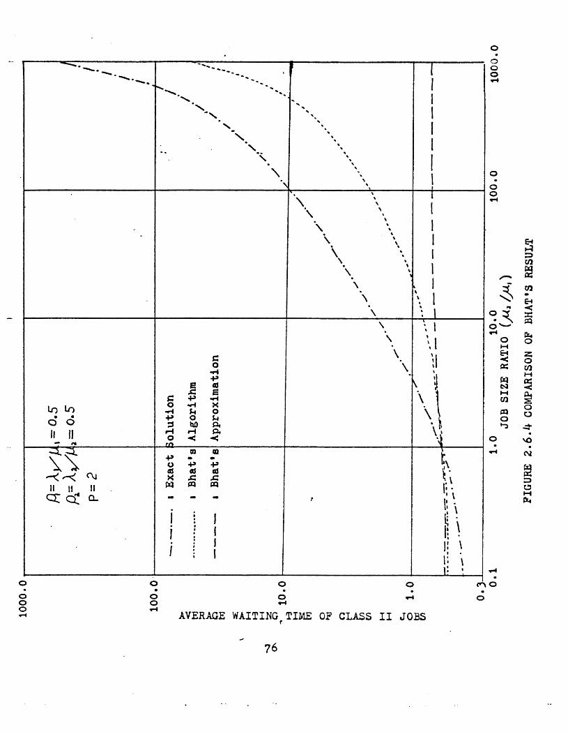
0
o
• "b_.̧
• _
\" "" 1\
_ "k O
. , ! _% 'bl 1• 0
"\ _, !'\"\ !
"\ , I _
• I, ?_ o
\ :l o
"\- ",l o_ o
= \ il _ =• "_ 0o \ =
i--4
- _j.p
0 _ _ . QLO I_ _ r_ o m c__c_ .P o _ o
0 ,_ .,_ 0 ,,0
'k ° ; ;il II !1 _1 _ _ I-4
i I!• ' I
i I ' "_'.!i ,
_; g g ,-; d
AVERAGE WAITING TI_E OF CLASS II JOBS
76

CHAPTER 3 Memory Mana£_,ement for Dat? Buffers
3. i. Introduction
]n Chapter 2, the waiting time for data packets was calculated. In ordinary
M/M/c or M/G/c queueing systems when the waiting space is several times larger than
the average queue length, the infinite queueing space assumption turns out to be good
a approximation, But, in the case of the integrated switch, the variation of queue
length is very large when the number of background Class [ jobs varies. The queue
length of Class 1! jobs will increase almost linearly with respect to time in some period,
and the conditional mean queue length may be much longer than total mean queue
length. In the under-loaded states, infinite queueing; space mig,ht well be a F_.,ood
approximation, while in over-loaded states this assumption becomes questionable.
When the number of packets requesting the service of the switch is Isreater than the
number of packet buffers in the switch, incoming packets will suffer extra delay: They
will experience a retransmission time because no empty buffer in the switch as well as
the waiting time for all the packets before it to be processed. ]n packet-switching, an
incomin G packet without a buffer is not acknowledged, so this packet will be sent
a_ain. Packets requesting service of an over-loaded switch have to suffer this extra
delay of re-transmission. In this chapter, finite memory space is assumed, and the
mechanism and the performance of memory managements as a means of decreasing or
eliminating packet delay are discussed.
There is a finite memory space M. When a packet comes in, it is assigned a
buffer if one is free. There are many approaches to assigning the buffer from the
• ??

memory, and there may be a secondary storage for packets during the period of over-
loaded states. Before the details of memory manaBement are discussed, one
assumption is made: The holding time for Class I job is so Ion 8 that the transient of.
changing [he number of Class | jobs is relatively shorl_ in fact, it is negliBible in terms
of the whole system behavior. Thus the switch is assumed to be in one steady state
followed by another with different service ability for Class ]I data packets.
An incomin 8 packet is either allocated a buffer or blocked. If a buffer is
assi6ned to a packet, thai buffer is called occupied_ otherwise it is free. An occupied
buffer is freed after its assiF_,ned packet is processed, transmitted to the next node,
and 8iven a positive acknowledF, ement. This whole period is called the life-time of the
buffer. If a packet can not be allocated a buffer, the switch behaves as if it has never
received that packet. No acknowledgement is sent back to the sender, and by the hi6h
level control protocol, this packe| will be sent by the sender again after a wailing
period. Although this data packet is not lost, it does suffer an extra delay. Because of
the above properties, the performance criterion used in this chapter is the probability
of packets being blocked. Another criterion, memory utilization or buffer utilization, is
also used in some sections.
Let us review the parameters of the integrated switch. It is a communication
system for voice and data. [t has very strict real time constraints. Because the
system sent out a frame every frame period, say of 10 milliseconds, any memory
manap=ement which needs more than a frame period to complete is not acceptable.
Only simple memory manas;ement schemes can be used. Secondary storaF, e, say a disk,
will 8enerally have access time in the order of tens of milliseconds, so a direct use of
disk for input and output will be inadequate. On the other hand, if the di_k is not
78

directly used in I/O but used, instead, in storaBe of the excess data packets, |han it
may well be effective. The access time for secondary storag, e may be less than the
extra delay suffered by the blocked packets. According to the SENET implementataion,
no processes can be overlapped when the input trunk line is writing into the input
frame buffer or when the output trunk line is sending out information from the output
frame buffer. Thus the extra delay for blocked packets, which is at least a two-frame0
period, will be in the order ofk 30 to 50 milliseconds. Apparently, with good use of
secondary storage, fewer retransmissions wilt occur and the Class I[ data packets can
have a smoother flow and a shorter delay.
|n the second section, several buffer management methods for primary memories
are tried. |ndependent exponentially distributed random variables for the life time of
buffers are assumed. The effectiveness of these managements methods are compared.
In the third section, a network model is built for buffered packets flowing in the
communication network. Closed queueing network model of exponential server are
solved by using the algorithm of Buzen[Buze 73]. In section four, secondary storage is
modeled. A forward and backward ali_orithm is developed to analyze the effect of the
secondary storaBe.
?9

3.2. Node Model
A finite memory of size Mis assumed in the intesrated switch. When a packet of
size r comes in, how should it be assigned a buffer? Because of the real time
requirements of the system, only several simple memory manaF,ements are relevant to
our attempt to answer this question. These include division of memory into maximum
size buffers, division of memory into several different fixed size buffers and dynamic
allcoation of first-fit memory are discussed. We will let D indicate the upper bound of
packet size; N=M/D, the number of buffers if all buffers are maximum size. First we
will discuss the system with N buffers of size D. In this system, an incomin8 packet,
re_;ardless of its size, is assis;ned a buffer until all the buffers are occupied. Then a
system with N! buffers of size M 1, Nz buffers of size M2,. ,. ,., and Nk buffers of
size M k is discussed, where MI<M2< • <. <. <Mk=D. There are two disciplines, static
and dynamic, for buffer assisnment when a small packet comes in while all
corr_.spo.ndirtg size buffers are occupied. We can either assiF_,na larF=,er buffer to the
packet or just block it. Finally, we explore a relatively complicated first-fit dynamic
memory allocation scheme. The input stream of data packets is assumed to be Poisson
and the buffer life-times are independent exponentially distributed random variables,
regardless of their size. 0
3.2.1. Maximum Size Buffers
All the buffers are of size D, the maximum size a packet can be. A buffer in the
memory is either free or occupied:
"i -!o o - N-iO O
.... C _ _ / 0
,,
OCCUPIED BUFFERS input with rate ,_REEBUFFERS
8O
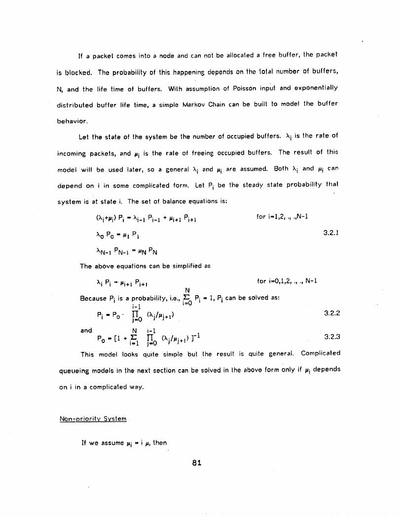
If a packet comes into a node and can not be allocated a free buffer, the packet
is blocked. The probability of this happeninl_ depends on the total number of buffers,
N, and the life time of buffers. With assumption of Poisson input and exponentially
distributed buffer life time, a simple Marker Chain can be built to model the buffer
behavior.
Let the state of the system be the number of occupied buffers, x.i is the rate of
incoming packets, and #i is the rate of freeing, occupied buffers. The result of this
model will be used later, so a general Xi and _i are assumed. Both gi and jui can,
depend on i in some complicated form. Let Pi be the steady state probability that
system is at state i. The set of balance equations is"
(X'i+#i) Pi - X'i-I Pi-I +/Ji+l Pi+l for i.-1,2,., .,N-1
X'o Po = Pl Pl 3.2.1
X'N- 1 PN- 1 = #N PN
The above equations can be simplified as
;ki Pi = Pi+l Pi+! for i=0,1,2,.,., N-1N
Because Pi is a probability, i.e., i50 Pi = 1, Pi can be solved as:i-1
Pi = Po' j]"_=O(XJ/'UJ+t) 3"2";'_
and N i-1
Po = [1 + i=lZ; j]'_=0 (X'J/"J+l)]-1 3.2.3
This model looks quite simple but the result is quite general. Complicated
queueing models in the next section can be solved in the above form only if #i depends
on i in a complicated way.
Non-priorit'l System
If we assume Pi = i #, then
81

i
Pn = (X/")n/n !" Po 3.2.4
where n
Po= [ i=_O(xh')i/i !]-l
The Erlang 2 formula, E2(n,X,,), is the Pn with input rate X, service rate # of a
M/M/n/n queuein 6, system. Then from simple arithmetical manipulation we can 6et:
E2(n+t,X.,,) = [t + (n+1),/X. / E2(n,X,,) ]-1 3.2.5
The buffer utilization factor R is defined as:n
.,:E J pjR j=t
= X./(n;j) [I-E2(n,X,_) ] 3.2.6
Notice that R is the utilization factor of buffers not the real utilization of the
memory. The real memory utilization factor will only be half of R if the packet size is
uniformly distributed between 0 and maximum size D.
Reserve Priority System
A simple reserve priority system is considered here. Suppose that there is a
probability o_ that an incoming; packet has hi6her priority, and that the life time of
buffers assigned to a hish priority packet is the same as that of other buffers. When
the number of buffers occupied is more than Nt, a packet will be allocated a buffer
only if it has hip__.hpriority. No preemptive of buffer is allowed. For low priority
packets the system has only N! buffers, but for hish priority packets the system has N
buffers. Equation 3.2.2 can be used with the followini_ definition of ;ki and jui :
X O<i_<N1Xi = { 3.2.7
o(.X N]<i__-N
82

If Pi is the probability that the system is in state i, then the blocking probability
for high priority packets is PN' and the blocking probability for low priority packets isN
Pi' Figure 3.2.1 shows the effect of this priority assignment. Under a heavilyi=N!
loaded situation, k/p_80, N,=30, a litlle extra buffer reserved for higher priority
packets will decrease the blocking probability greatly, from 0.63 to 0.04 with N1=28.
3.2.2. Different Fixed Size Buffers
Instead of dividing the whole memory into buffers of maximum size, the memory
is divided into fixed size buffers of more than one size. When a data packet comes in,
an attempt is made to allocate a buffer of corresponding size to that packet. If all the
buffers of corresponding size are occupied, there will be two disciplines, the packet
will either be blocked or assigned a larger buffer. We call the first discipline, static
t ,
assignment! the second, dynamic assig,nment.
Static AssiKnment
There is a corresponding set of buffers which can be assigned to every packet..
Suppose there are d different buffer sizes, each of size Mi, i==1,2,.,., K, and MI<Mz< "<k
• <Mk. There are Ni buffers of size Mi, i51Mi • Ni _<M. Any packet of size in the range
(Mi_l, Mi] is treated as a packet of size Mi and is assigned to a buffer of size M i.
Because of the simple discipline for buffer allocation, the blocking probability for"
packets of size Mi is independent of the allocation of buffers to packets of other sizes.
Let :x.i be the Poisson input rate of packets of size Mi. With the assumption that tho
life time of a buffer is independent of its size, Bi, the blocking probability of packets of
size Mi, is of Erlang 2 formula=
Bi = E2(Ni, Xi, _u) 3.2.8
83

1.0 ..... Y t ! _ I-''-.. Blocking Probability for
- Low Priority Customers
"_ •
" /,_, ,e
0.9 - .. /N = 30 Total Number of Buff_s -
. /.
(3( 10% Percentage of High "-. ./Priority Customers . /
o08 " " "
= 80 /-_
Q = 1.0 / \._0.7 - / \0
_'_ o •
/
/ U_ilization Factor !
0.5 / R _,• I
" / l./ I
/ l
0.4 - ./ I/ !
/ I/ l
/ I
0.3 - /-/ i._o l
0.2 /_ j.• Blocking Probabaility j.
for High Priority lO.1 - Customers l
lil
//
0 | ! I i i -- "_ i
2 _ 10 14 18 22 26 30NUMBER OF BUFFERS CAN BE OCCUPIED BY LOW PRIORITY CUSTOMERS
FIGURE 3.2.1 PERFORMANCE OF RESERVE PRIORITY BUFFER SYSTEM
84

The tolal blocking probability becomes:k k
= _ x.i E2(Ni.,_.i,_) / X 3.2.9B = i=_1 (Xi/X') " Bi i=1 k
where X. is the total input rate and X. = i_=1Xi.
Then Ri, the buffer utilization factor for size Mi, becomes;
Ri = X.i[ 1 _ Ez(Ni,ki,_j) ] / (Nile) 3.2.10o
The numerator is the effective number of buffers allocated per unit time, and
the denominator is the effective number of buffers available per unit time. The total
buffer utilization factor, R, is:k
R = _' Mi- Ni- Ri /Mi=1
k
= _ MiX i[1 -E2(N i,X i,#)]/(M_) 3.2.11i=1
From the above definition, an optimum assignment of Mi, X.i and Ni to minimize B
will in general differ from that required to maximize R. Instead of creating a larger
buffer, more small buffers will be created. Although this may decrease the total
blocking probability, it also decreases the total buffer utilization. In addition,
minimizing; the total blocking probability may favor small packets. In some situations
the optimum assignment of Ni will give a blocking probability of 1 to large packets.
Before a better criterion can be found, the blocking probability and buffer utilization
factor will be used for evalution. Almost all buffer management schemes favor packets
of small size over packets of large size. Figures 3.2.2 and 3.2.3 show the op|imum
assignment of N! and N2 for both minimizing B and maximizing R respectively. Two
size buffers are considered, one of size MI and one of size M2=D, the maximum size of
a packet. A uniform distribution of packet size is assumed, i.e.X.I=XMI/D, and X2=X-NI,.
where X is the total input rate Qf packets. The number in the bracket of the fisure is
the corresponding number of N! and N2 for the optimization assignment. Figure 3.2.4
@5

=4f
003H
_" (31,;:¢.zo,29) .--"h:/ "
o o.2- --.(_5,271 .--- 0,6)
> --.. (16,25) j 22) -----;4('28", 9),. -_. _ 20,' -- - -,-.-_.-'_,Ts)i Minimum Blocking PrObaD111_yi
_ 0.I I I , , i I ,
1.o 2.0 3.0 4.o 5.0 6.0 7.0 8.0 9.CSMAI_L BUFFER SIZE (MI) .,WITH MAXIMUM BUFFER SIZE (M2=IO) ANDTOTAL _[EMORY UNIT (M=300)
FIGURE 3.2.2 STATIC BUFFER ASSIGN_ENT AT HEAVY LOAD
r
86

(N1,N2) = (Number of Small Buffers,_Number of Large BuffersI
= 20.0
=I.0 .....
w M2= 300
o M = 10_o.o2 ......_D
'_ (27,5o Minimum Blocking ..-"
0.01 Probability _ if6,9)
t-,H Llo,29) - -_'_,13,)_Io.2B).(,16.21)_(3.v-_l_(_o-,.7_)-f25,_)
0 -- i1.o 2.0 3Lo 4_o 5'o. 6.'o ?.o 8.o 9.o
_ SMALL BUFFER SZZ_ (M1)
WITH MAXIMUM BUFFER SIZE (M2=IO) AND TOTAL MEMORY UNIT (M=300)
FIGURE 3-2.3 STATIC BUFFER ASSIGNMENT
87'

1.0, I t _ 1 I .
/ -Total Memory Unit M=300
0.9- Large Buffer Size M2=IO
Small Buffer Size M1=5
_- 2o. _= I.o0.8-
g , Blocking Probability for Large Packet
0.7 - _ , Blocking Probability for Small Packet -O
A
c_0.6 -
0
Utilization Factor___- _.
/\
.._n.a,_ \ -
\ /,,"k / /
0.3 - _. • -
,,- \ _ / ./, \ // "\ A " -
0.2 _ / //\ /Total Blocking_ \
0.1 - Probability "\, "),_.
N2, ) 5 I0 15 20 25 30N1,60 50 40 30 20 10 0
NUMBER OF BUFFERS, LARGE AND SMALL
FIGURE 3.2.4 STATIC TWO SIZE BUFFER ASSIGNMENT
88

01 9. i
0 _ - ,_ ...... ._, •,_,,c _" i0 2b 2_ 3N:, 60 50 40 30 20 I0 0
NUMBER OF BUFFERS, LARGE AND SMALL
FIGURE 3.2.5 STATIC TWO SIZE BUFFER ASSIGNMENT AT h_AVY LOAD
89

and 3.2.5 show the blocking probabilities and utilization factor when we have M! equal
to D/2. Comparing the three figures, we see thai the choice of the size of M 1 is not
very critical as long, as an optimum combination of N 1 and N2 can be found. But for
fixed MI, the choice of N! and N2 is rather critical. For a lightly loaded system, the
optimization assignment of N! and N2 are the same for both minimizing [3 and
maximizing R.
Dynamic AssiF,nment
Now we consider the system thai allows large buffers to be assigned to small
packets if no small buffers are available. The definitions of Mi, Ni and Xi used in static
assig,nment are also used here. A small packet is blocked only if all the buffers are
occupied. A large packet is blocked if no large buffer is available. Apparently, the
system is heavily biased in favor of packets of small size. There are many reasons for
using such system. For example, as we shall see later, in addition to being relatively
simple, it gives better throughput, a lower lotal blocking; probability, and a higher
buffer utilization factor. As we witl see later, in some situations this buffer
management scheme is better than the static assip_,nment scheme.o
A two-dimensional Markov Chain is built for a system with two buffer sizes,
large and small. The state space of the Markov Chain is S={(i,j) I i,j >0}, where i,j
indicates the number of small and large buffers occupied, respectively. Notice that the
state is not defined by the number of packets of relative size, because some small
packets may occupy large buffers. No reassignment of buffers will be made if some
small buffer is freed after a small packet has already been assigned a large buffer.
Figure 3.2.6 shows the probability transition flow of the Markov chain. The horizontal
9O

transition rates, i.e., transition between (i,j) and (i,j+l), are ;_2 and (j+l)#, except for
the last row, where i-N, and the lart_e buffer will be assigned to the small packets too.
FIGURE 3.2.6 STATIC SPACE 0P DYNAi_C ASSiGND_ENTOP BUPPERS
The balance equations are
[;kl+X'2+(ii.J)_] Pi,j = klPi-l,j + X'2Pi,J-1 + (i+l)/_Pi+l'J + (J+l)PPi'J+l
for O<i<N 1, O<j<N2 3.2.12
for i=-O, j,=O, tt_ first and second term of the right hand side vani._h,respectively.
[kl+X'2+i_] Pi,o = ;'lPi-l,0 + (i+l)_Pi+l, ° +_'Pi,o for 0<i<N 1
and
[kl+X'2+J_3 Po,j = X'2Po,j-] +/_PI,j . (J+I)PPoj+I for 0<j<N 2
[)'1 + ;k2_ _0,0 '= PPt,0 + #Po, I
for j = N 2, the- iast term vanishes,
[XI+(i+Nzz:] Pi,N 2 = XIPi_I,N2 + ;k2Pi,N2_.l + (i+I)pP{+I,N2
Note that for i =NI, the transition flow is different. There is no small buffer
91

available, so any new small packets will be assigned a large buffer until all larger
buffers are also occupied. The transition rate from (N1, j) to (NI,J+I) is (),l+;k2), instead
of X2. And the balance equation becomes:
[XI+X2+(NI+J).u]PNI,j " XIPNI-I,j + (XI+X2)PNI,j_ 1 + (j+t),uPNI,j+I
for O<j<N2 3.2.13
And for j=O and j=N 2, the balance equations become:
[XI+X2+NI#]PNI,O = X'IPN!-I,O + #PNI,I
(NI+N2)# PNI,N2" XI PNI-|,N2 + (A.I+X2)PNI,N2-1
The above set of equations can be solved by the constraint that Pi,j are
probabilities, i.e., ._. Pij = 1. A straight-forward Gauss-Seidei algorithm [Ra169] is usedIj
to solve the system, and some results are shown in figure 3.2.7 and 3.2.8. The
blocking probability for small packets, B1, is equal to the probability PNI,N 2 and the
blocking probability for large packets is equal to summation of Pi,N2 over all i.
The Gauss-Seidei algorithm needs a space of (NI+I)X(N2+I), and its convergent
rate depends also on N 1 and N2. For N|, N2 less than 100, the algorithm will converge
to an error of less than tO (-4) in less than several minutes of CPU time on a PDP-10.
But for large NI, N2 or of system with k different size buffer, there will be some
difficulty in calculating the exact probability distribution. Two approximation formula
are suggested below.
Let us model the system as seen from the perspective of the large buffers.
During one period the stream of requests is Poisson input of rate XI+X 2, while durin_
the other period the request stream has an input rate of only X2. FiF_,ure 3.2.9 depicts
its input rate of the queueing system.
92

1.0 I I i _ I _ t I J
To_al Memory Uni_ M = 300,
- Large Buffer Size M 2 = 10, -
Small Buffer Size M1 = 5.
= 4o, = 1.00.8-
--------s Exac_ SolutionO
_ . - .... , Estimation0
, Large Buffers
o ' _ , Small Buffers>.
0.6-'L-.,I-4"3
0.2
O, I ' I I I ' ' ' 2_N, s 2 4 _ 8 10 12 14 16 18Na, 30 29 28 27 26 25 24 23 22 21 20
NUMBER OF BUFFERS, LARGE AND SMALLf
FIGURE 3.2.7 DYNAMIC ASSIGNMENT OF TWO SIZE BUFFER
93

! I I, I I _ '- I
0.1 ---" I. To_al Memory Unit M = 300
Large Buffer Size M 2 = 10, . -
Small Buffer Size M 1 = 5-
k =zo. y--1.oreel
___ .m_ _
0 • 01 "*'_ " _ "
Large Packet %% -
g= _m
0.001
, Exact _% X _ i _// -
----- , Approximati
Small Packe't"_X -
0.0001 _ i - l _ " l "' "' ..X_
N2 I 30 29 28 27 26 25 24 23 22 21 20
NUMBER OF BUFFERS, LARGE AND S_]ALL
FIGURE 3.2.8 DYNA_ilC ASSIGN],iENTFOR TWO SIZE BUFFER
AT LIGHT LOAD CONDITION
9_

xl*x2X2
\ \ \ \ _\\ • \ \
FIGURE 3.2.9 ]NPUT RATE OF THE QUEUE
During the period indicated by shaded area, the request rate for large buffers
increases to (kl+kz); otherwise the rate remains ;k2. The shaded area depicts the busy
period for the M/M/NI/N ! queueing system of small buffers. In general this period will
not be exponentially distributed, which implies that the system has quite complicated
input states. We know, however, that the ratio of the shaded period to the whole
period is x==E2(Nl,;kl,p), the busy probability for the M/M/NI/N ! queueing system of
small buffers; If we keep this ratio x constant, but shrink or expand the duration of the
shaded period and the non-shaded period, two approximation formulas are derived:
(P1) Keep the ratio x constant and let the duration of the average shaded period go to
zero. The system becomes an M/M/N2/N 2 queueing system with the same
service rate but an input rate of (X2+XI.x). Thus the blocking probability for
large packets becomes E2(N2,X2+XI.X,p).
(P2) Keep the ratio x constant and let the duration of the shaded period go to infinity.
The system will have a negligible transience from one M/M/N2/N z queueing
system of input rate ;_2 to another M/M/N2/N 2 queueing system of input rate
(_I.X2) and back and forth. T.he blocking probability for large buffers is the
average of these two : xE2(N2,X.I+;_2,#) + (l-x) E2(N2,X2,p).
95

Figures 3.2.7 and 3.2.8 show the bloc:king probability for both small packets and
large packets and the two approximation formulas. When the syslem is lil_htly loaded,
the values of the above two formulas will be quite far away from each other, as shown
in FiGure 3.2.8, and the exact value will lie somewhere between ihe extremes. But for
a moderately loaded system, i.e., X=40, the values of the approximation formula are
quite close, and both are good approximations of the exact solution, as Figure 3.2.7
shows.
Comparin_ Fil];ure 3.2.8 with Figures 3.2.2, 3.2.3 and 3.2.4, for li_,htly loaded
systems, we find that the dynamic assignment system becomes the superior scheme. In
the moderately loaded system, however, FiF,ures 3.2.7 and 3.2.5 show the value of the
dynamic assignment is questionable. For a lig;htly loaded system, :k = 20, the optimum
assignment of N], N2 for static assiF_,nment will get a blocking probability of 0.00187
for both large and small packets. For dynamic assignment, N1=14 and N2=23 will give
a blocking, probability about three times better for packets of both sizes. For a
moderately loaded system, X. = 40, the dynamic assignment is strongly biased in favor
of small packets. Large packets will always suffer a high blocking probability. For
dynamic assignment, B2, blocking probability for large packets, can never be lower
than O.21. For the static assignment, the blocking; probability can be BI=B2=O.16 for
both small and larg;e packets. Thus if the system need_ a relatively balance bloc:king
probability or has an upper limit blocking probability for all packets, then dynamic
assig;nment may not be proper under some loading; condition.
3.2.3. Dynamic Memory Allocation
There are many similarities between buffer management in communication
96

0.5 ....... Y ......... I ! t i t ! -
Total Memory Unit M = 256
Maximum Size of Buffer D -- 8.
.... , k = 5o, ._ = I.o
..... , X=_o, _-z.o /I0._ - l-
,,, ..... , _=30. ._=z.0t'l ""- I0CJ I
II-.I I
Q i
'rl II
0 Ii_l - I>" II_1 1I-4 I -
0.3 -I-4
l
ll
llIl
l
0.2 - / l"/ /i /
Least Blocking Probability Reachable /, /By Fixed Size Buffer Assignment t //
li /................. /- ........... ./-.....
O.I - / ./_ -
/ z.// _'_ _/"Dynamic
// _ Memory Allocat .oni /
/ /
t . "- "j/ 0/
/ /, ..-_ ..,Is ..j og/
0 - r "r ..... _,' , "C I 2 3 _ 5 6 ? 3
BUFFER SIZE
f
FIGURE 3.2.10 COMPARISON OF FIXED SIZE BUFFER ASSIGh_ENT AND
DYNAMIC MEMORY ALLOCATION
97

systems and memory mana[T,ement in multi-programming computer system. All buffer
manag;ement schemes discussed here are very simple, because of the strict real time
requirement in the communication environment. Now we will consider a more
complicated memory management commonly used in the large computer system:
dynamic memory management. There are many well-known algorithms, such as first-fit,
best-fit, buddy, etc.[Knu68]. Each has its own characteristics and fils best into a
specific environment. For the communication system in which simplicity and reliability
are the most important requirements, a first-fit algorithm is tried and simulated for the
buffer management of the communication system.
The first-fit algorithm used here is very similar to that mentioned in Volumne 1
of Knuth[Knu68]. The whole memory is divided into blocks dynamically. A block is a set
of contiguous memory locations which are either free or belong to the same packet.
There are two types of blocks, free or occupied, and every block is linked to another
to form a set of ring buffers. There are four fields for each block: block size or
starting; address of next block, starling; address of the next same type block, starting,
address of last block, and starting address of the last same type block.
free block occupied block
size pointer to next blockpointer to next free block pointer to next occupied blockpointer to last block pointer to last blockpointer to last free block pointer to last occupied blockbuffer buffer
All the buffers, free or occupied, are linked together. Another pointer, AROV,
points to the currently free block, and from this place the next incoming packet will
begin to search for the first large enough free block on the free buffer ring. Because
98

of the ring: structure, two flaEs, FEMP and BEMP, are needed to poinl out whether
there is any free block or occupied blocl_ in the system. FEMP=I if there is no free
block, and BEMP=I if there is no occupied or bounded block.
The detailed als;oirthm can be found in [Knu68]. Only the blocking: probabilities
are compared here to other buffer managements techniques. The simulation resut|s,o
Figure 3.2.I0, shows the blocking probability for packets of different sizes. This
scherne also favors smaller size packets over larp,,er ones. This complicated memory
manasement scheme offers a lower total blockin8 probability than all other schemes
we have discussed, but it is also the most complex one.
99

3.3. Network Model
In the last section some buffer manas;ement techniques were tested. The life
time of buffers is assumed to have an Exponential distribution with mean pi=i/J. Tills
assumption will be justified, and the conditions under which the assumption holds will
be also discussed in this section. First we will explain the model as follows:
X p
, _. _.
_4 /a3 #2 Y
C)-[I II<, . I I1<.....!o o o o o o <
_k-1 P k-2 P k-3
A closed queueing network is used fo model the buffer behavior of the current
integrated switch. The number of customers in the queuein8 network is the total
number of buffers, occupied'or free, in the integrated switch. Customers in service
center SK are the free buffers of the switch; all other customers are buffered data
packets. Customers in service center S! are packets which have been assi6ned
buffers and are awaiting the processinp_, in the current intep:,rated switch. Those
buffered packets are then transmitted, with probability Pl, throup_h transmission line
$2, to the next integrated switch, S3, with probability Pr, through SK_3, SK_2, etc.
After the customers undergo the necessary processing in the next switch, S3, the
100

correspondint_ positive acknowledF.,ements are sent back, through $4, to the current
switch. When the current switch receives an acknowledgement, the buffer of the
packet begin acknowledged is released and a new free buffer is created in SK. Whet,
the number of customers in SK is also zero, i.e., there is no free buffer in the current
switch, the output rate of SK is zero. This implies that all new incoming packets will be,
blocked because there are no free buffers, so it looks as if there are no new incoming
packets. The service discipline for all service centers is FIFO (First In First Out).
There may be one or more servers in a service center, and each service center may
have different service distribution.
First the exponential servers are assumed, then a network mixing two kinds of
customers is modeled and simplified. Later in the section, the service centers, S2 and
S4 are modeled as delay lines rather than ordinary queues.
3.3.1. E.xponentiat Oueuein_ Network
Suppose there is a total of M customers in the closed queueing network and K
service centers, S1, S2,',', SKwithcl,c 2,.,',c K servers, respectively. One customer
can not be serviced by more than one server, and has no preference for any server',
since all servers in the same service center are identical. The service time at service
center Si is an exponentially distributed random variable with mean t//= i, i=1, 2,., K.
All the customers are identical too, and the state of the system is the number of
customers in the service centers. The steady state of this kind of exponential
queueinF_, network was solved by Gordon and Newell IGor67]. The probability that the
system is in a specific state has the product form. Let ni be the number of customers
at service center Si. Let the state of the system be (nl, n2, ., ", nK). Then the
equilibrium probability that the system is at state (n 1, n2, ", ', nK) is
101

t
K
1 _ (Xi)niP[n]'n2' "' "' nK] ""G(M'--) 1 / Ai(n i) 3.3.1
K
where .._ n i .- M andK
#jXj = i_l= _iXiPi,j j = 1,2,3,.,., K.
where Pi,j is the probability that a customer will proceed to the jth service center
after completing a service request at the ith service center, and 1/_ i is the average
service request at service center Si. G(M)is the normalization constant so that the
summation of P[nl,nz,.,-,nK] over all feasible states is one, where the feasible statesK
are defined such that _ ni = Mand ni>_Ofor all i=1,2,.,-,K. That isi=1t,
K
G(M) = n(S(M,K)_ _1 [(Xi)ni/ Ai(ni) ] 3.3.2
K
where S(M,K) = {(nl,n2,.,-, nK) J i=_[ n i = M and ni>O for all i}, and Ai(n i) is defined
recursively as follows:
Ai(O)=t
At(j) = J Ai(J-1) if j<c i
At(J) = ct At(J-l) if j>_ci 3.3.3
where ci is the number of servers at service center Si.
An alBorithm was derived by 8uzen [Buz73] to solve the above problem. A
temporal variable, g;(m,k), is defined as:k
_'_ _1 (xi)nig,(m,k) = / Ai(n i) 3.3.4n(S{m,k)
Note that G(M) : 6(M,K), and in fact g(m,K) = G(m) for m=O,t,2,-,. M. From the
above equation:
g(m,1) = xlm / Al(m) for m=O,t ,2,- ,-,M 3.3.5
and g(O,k) - 1 for k=O,l,2,. ,. ,K
with the recursive formula of g,(m,k):
102

rn
g(rn,k) = j_=l [(Xk)j / Ak(J)] " 8;(m-j,k-1) 3.3.6
B(rn,k) can be calculated. Only 2(M.1) memory space are needed to store p_,(m,k-l) and
to calculate 6(m,k) for rn=0,1,2,3,.,. M.
The rnarsinal probability, PK(j), is calculated
PK(j) = j customers at service station SK
= [(XK)J / AK(j)] " g(M-j,K-1)G(M)
= [(XK)J /AK(J)] " B(M-j,K-1) 3.3.7' g(M,K)
Define throup=hput TK(rn) as the rate of which customers pass through service
center SK when there are rn customers in the queueinB network and the service time
at service center SK is reduced to zero. Then TK(m) becomes.
TK(m) = XK • B(m-l,K-1) / B(m,K-1) 3.3,8
By Theorem 1 of [Cha75], the effect on the queuein8 network with resard to service
center SK is equivalent to the followin 8 load-dependent queueins: network.e
•._ .u
TK(i)
TK(i) is the load dependent input rate of a sin_;le queue.
i jobsTK(M-i)
.....>' ' ''_--(, _KI' ' ' ' "-" >IIII _j"
103

where TK(O)=O. The probability that a service center SK has i customers is:
i-1
PK(i)" PK(O)' J_=O [TK(M-J) / _K(J)] 3.3.9
whereM _-1
PK(O) = [1 + i=l_' j]_=O {TK(M-J) / _'K(j) }]-1
which are exact in the same form of equation (3.2.2) and (3.2.3).
From the above derivation, we know that TK(j) works as an interface between
service center SK and the rest of the network. If service center SK is the free buffer
queue, then [1/TK(1) ] is the average life time of an occupied buffer, and the
assumption of last section can be simplified as
TK(i) = i- TK(1) 3.3.10
Now we consider the more complicated network in which the integrated switch
S3 has other work to do besides processing the packets coming from integrated switch
Sl. Here there are streams of jobs flowing into switch S3, requesting service, and
leaving the queueing network. The queueing network becomes:
--ill/'14 P3 P2
There are two kinds of customers. One kind includes the buffers of the current
integrated switch and the corresponding packe|s; the other kind includes those
10g

requesting service to switch S3 other than the packets sent from switch Si. Sz and S 4
are assumed to be the trunk lines between integrated switch S1 and S3, SK is the free
buffer queue of the current integrated switch S1. Let us represent the network as the
left network of the following figure, and prove that the two networks are identical as
far as the first kind of customers is concerned.
X p X. p
-llil-Q ,lii -\
s, (:,-'r)
\, ...... (5>-fIl .....
Let i l, i2, i3 be the number of customers of first kind in service centers S l, S2,
$3, respectively. Let J2 be the number of customers of second kind in service center
S2. The service requests for both kinds of customers are the same exponentially
distributed random variables. The service discipline for both kinds of customers is the
same F]FO. Then, by the technique of independent balance equation developed by
Baskett et al. [Bas73], the equilibrium state probabilities are of product form:
Pill, i2, i3, J2] = D hl(i l) h2(i 2, j2) h3(i 3) 3.3.1 1
where (il+i2+i3)=M, the total number of customers of the first kind in the queueing
network. And
hi(i) = (l/p) i
h2(i,j) = (i+j)! "F_'. (1/_')i " (_/v)J 3.3.12
h3(i) = (l/X) i
lo5
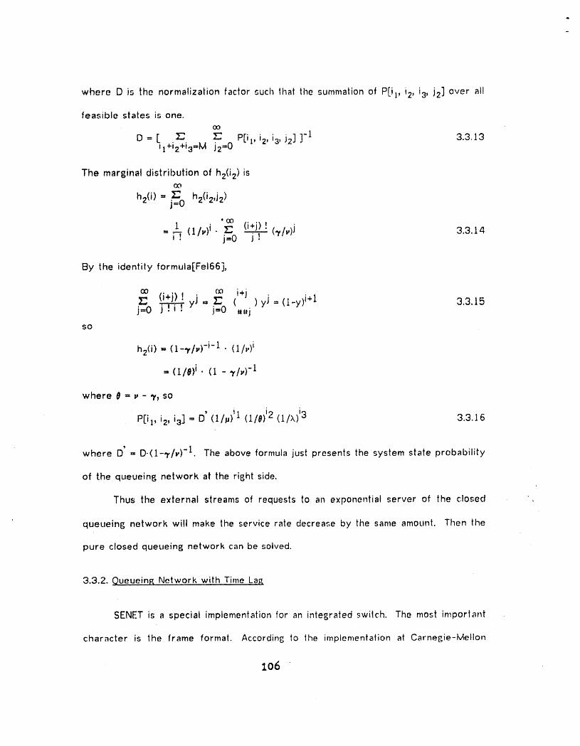
where D is the normalization factor such that the summation of P[i l, i2, i3, J2] over all
feasible slates is one.(30
D = [. _- _' P[il, i2, i3, J2] ]-1 3.3o13I l+i2+i3=M j2=0
The marginal distribution of hz(iz) is(3O
h2(i) = _ hz(i2,J2)j---0
I .oo (i+j) != _ (t/v) i- _.. (_,/,)J 3.3.14Jj=u
By the identity formula[Fe166],
oo _xl i+j,_ (i+j) ! yj ,, _, ( ) yJ = (l-y) i+1 3.3.15j=o j=o ..j
SO
h2(i)= (t-,r/v)-i-l (i/v)i
= (t/0) i. (1 - ,.r/v)-t
where 0 = v - ,,/_so
= D'p[il, i2, i3] (l/p) _1 (1/0) _2(t/X) _3 3.3.16
where D' = D-(1-,1,/v) -1. The above formula just presents the system state probability
of the queueing network at the right side.
Thus the external streams of requests to an exponential server of the closed
queuein6 network will make the service rate decrease by the same amount. Then the
pure closed queueing network can be solved.
3.3.2. Queuein6 Network with Time Lap,
SENET is a special implementation for an integrated swilch. The most important
character is the frame format. According to the implementation at Carnegie-Mellon
lO6

4
University [Bar76], the switch will have frame buffers. There is a finite delay for the
packing; of a frame, transmitting it, and unpacking it. The delay is at least two frame
periods, no matter how much processing power is available. Also there is the t_me
required for transmitting a packet from one switch to another. Transmission line, $2,
S4., ., • of the queueing network are actually more like a delay line. The queueing
network is redrawn as follow,_.
x, tJ
delay T1 /*3 .... delay T]
t t < lll L<Pio o o o o o ,<
_UK_2 i<
Service centers S],$3,.,., SK_2 are defined as integrated switches. After a
service request is completed, a customer, which is a buffered packet, is put into the
output frame of the switch. After some delay, the packet will appear in the inputt
frame of the next switch° The delay is defined as the period extending from the
moment the packet is copied into the output frame to the moment the packet is copied
from the input frame of the next switch. If the largest share of a buffer's life time is
spent waiting for service at integrated switches, then the input rate of service center
SK will be limited by the service rate of the integrated switch. On the other hand, if
the delay is much longer than the waiting time and service time in the integrated
switches, then TK(i) will be proportional to i.
1o?

The delay line can be modeled as an Ivi/G/ooqueue. The customer encounters no
waiting time; service time is the delay. Closed finite queuein6 networks wilh this kind
of delay was studied by Posner and Bernholtz[Pos68]. The derivation is very involved,
but the result is quite simple and powerful. The result has the same product form as
the exponential queuein_, network, but the delay may not be exponentially distributed.
Only the averaBe delay enters the formula.
P[nl,n2,., .,nK] = D hl(n l) hz(nz). • • hK(nk) 3.3.17
If jth station is a delay line of averap=,edelay Tj, then
hj(nj) = (Tj) nj / nj! 3.3.18
Define Pi as the probabiliLy that a packet will 6o to the correspondin_ i switch
when it finishes the processin6 of the current integrated switch. The equation can be
more simplified.
hd(n d) = T nd /nd! 3.3.19
where nd is the total number of customers in delay lines rather than in the integrated
switch, andr
T=_i=1 piTi
is the avera6e total delay. The state probability of ni customers in ith intesrated
switch becomes
P[ni, for alt i such that Si_{switch}]
= D [ I]7_Shi(ni) ] hd(n d) 3.3.20
where i(_S ni + nd = M, total number of customers in the network. S is the set of
service centers of the queuein 6 network which are referred to the integrated switch
of the real communication system.
108

3.3.3. Numerical Results
Figure 3.3.1 shows the throughput with respect to i. Here the delay line model
of the last section is used. The delay time is set to be 15 milliseconds. The curves
show the processing capability for the switching processors. When the switching
processor can process four packets during each 10 millisecond frame period, the
throughput is almost linear. ]f the switching processor can only process one packet
for each frame period, the throughput reaches a maximum value very rapidly. The
throughput is now limited by the switching processor and most of the buffers are
queued in the system and waiting for processing rather than being transmitted in the
communication links.
T(i) increases almost linearly with respect to i when i is small; it rapidly
approaches to a limit value when i is large. T(i) can be approximated by the following
formula.
T(i) = minimum of (ib, I-) 3.3.21
where 1/b is the summation of average service time for a packet through the network.
There is a physical interpretation for this. When i is small, the packets are
widely scattered in the queueing network. The chance that a packet has to wait for
another packet is very small, so the throughput of the network increases linearly with
respect to i. When i becomes large, the throughput is bounded by the processing
capability of the nelwork, so the increase in the number of packets will not increase
the throughput. We will divide the curves into two regions= the customer-bounded
region, i<,r/b, and the processing-bounded region, i>l-/b, respectively.
The model we discussed in the last section is assumed in the customer bounded
region. In that region, the switch has enough processing power to process all the
lo9

incoming packets. The blocking of packets is due to the insufficient buffer spaces. If
the integrated switch is in the processin_,-bounded resion, the number of buffers is
not very critical. In an ordinary packet switching, networkp if the system is in the
processing-bounded res;ionj the network is con_;ested. For inte_;r_ted swilch, this
condition is called the over-loaded state, i.e., X>(c-icv). In the next section we will
discuss the use of a secondary storage in the processing-bounded re_ion.
110

o.5 t I , ! )/
/-/
/
Delay = 15 millisecond //
J
/
' , Multi-serversJ
l
O.LF- ---------, Unit-server ..,0 -- . --. i i I...._ ....-_;_-.'.-
Approxlma_1on _./..-_"
/" J .
/'/ i'_"0.3 - ."" ,'_"
./'_' /t
• ts _
/ ,, !. /
0.2 " / ,..-................. _....
o" ,',_'-__C)X = 2 Packets/10 millisecond/ ;f / /
/j.Y./ ,,;Y .: '
/'l
/;t"" I
/,"O ' ," I
o 5 _o z'5 20 25 36-
NUMBER0F BUFFERS(I)
FIGURE 3.3.1 THROUGHPUT OF NETWORK QUEUEING MODEL
111

3.4. Secondary' Storap,e Model
|n general, a communication processor will have a disk or a secondary storap_e
device if the processor has to manaBe a file system as well as perform its switching
function. For a pure switching processor, however, the speed of a disk is too slow to
meet the needs of a real time environment, so a disk is seldom used. For an ordinary
packet-switching network, like ARPANET, a disk is not necessary. Because the
expected waiting len6th of packets at the swilch is much less than the buffer space of
the switch, conB;estion will not occur frequently. Althoup_,h the function of the
integrated switch is similar to that of an ordinary packet-switchin_ network, we feel
that for the specific environment, a secondary storage device mil];ht be helpful. For
the intes, rated switch, the waitins; time has a very lar6e variance, and the expected
frequency of congestion is rather hip_,h. A con6estion of an integrated switch occurs
when it enters the overloaded states, i.e., when the input rate is hi6her than the
processins; capacity for the Class ]| packets. This will happen whenever i, the number
of Class ] customers, is above a certain level such that (c-i_Cv)#2<X.2. Once conp=estion
occurs, not only will packets passin6 the cons;ested switch be slowed down, but all the
adjacent switches will be affected. All the packets destined for the con6ested switch
cannot be sent out at res;ular rate, and the adjacent switches will have less buffer
space and processing power to process other packets. When the cause of the
con6estion disappears, some time is required to release the con6estion of the network.
because the expected frequency of the intesrated switch bein5 in the overloaded
states is rather hi6h, a secondary storap_,e device is sur_,p_,estedfor the integrated
switch. Such a device will prevent the adjacent switches from beins; affected by
152

congestion and speed up the recovery process after congestion. When the integrated
switch is in the overloaded state_ it can pump the excess packets into the secondary
storage device rather than block them. Although the packets will still suffer extra,
delay, time to transfer to the disk and back, an overloaded switch will not affect its,
neighbors by blocking the packets transmitted to it.
Whether to block a packet and let it be transmitted again or to accept it and pull
it into disk is unclear. For both cases_ the packet will suffer extra delay. A four-frame
period is usually required to make sure a packet is blocked and to transmit it again.
The transfer time to and from a disk is of the same order of maBnitude, so once the
situation happens, it is F=oing to suffer about the same amount of delay. There are
merits to blocking a packet rather than putting it on the disk, however. This is
especially true when the dynamic routing algorithm is used to determine the fastest
route for a packet. |t is hard to determine the response time if the next switch gives
a quick positive acknowledgement but puts the packet in disk for a long period. On the
other hand_ the use of a disk will relieve the congestion once it occurs.
3.4.1. Modeling
A model similar to a water container is used to model the secondary storage
device. The buffer space is modeled as the water container with input rate X. and
output (service) rate ,u. If the container is full, no more water can come in_ if the
container is empty, no water will flow out. Unlike an ordinary container with one input
pipe and one output pipe, this container is connected to an infinite reservoir through
two extra pipes at water levels N! and N2. When the water level is below N 1, another
water stream of rate _ will flow into the container. When the water level is above Nz,
113

a water stream of rate /_ will be pumped out of the container. The purpose of these
two extra pipes is to decrease the probability of the container being full and to
increase the usage and the tl'u'oughput of the container.
X
_---> dN2
L _ and from infinite
to an
J reservoir
--->p
Q
Returning to the integrated switch, we can let the water container stand for the
buffer space and let the infinite reservoir stand for the disk, the secondary storage.
and _ will represent the transfer rates to and from the disk. The secondary storage
is used only to store the excessive data packets, and a full parallel processing of the
switching processor and the disk controller is assumed. Whenever the number of
packets exceeds the limit N2, the disk will be enabled to transfer a block of data onto
the disk. When the number of packets in main memory is below Nt, the reverse
process occurs_ i.e., a block of data is brouF_ht back into the main memory. A block of
data moving; to and from the disk may contain one or more data packets. This model
reflects the nature of a communication procssor. Unlike most ]/0 queueing models of
large multi-programming computer, the data (packets) are not designated to any
specific users. Like the water in our analogy, which makes no distinction between
users, this model does not require that the user's space and the packets be monitored.
Every process is assumed to be memoryless, i.e., Poisson input process,
114

exponentially distributed service time and block transfer rates. A Markov chain model
is built as follows"
O(:
/.L"
The state of the system is the number of packets or the number of occupied buffers in
the system, where X is input rate of packets, 1/_, the average service time, ]./c,'_, the
average time to read a block of data from the disk, 1//3, the average time to write a
block of data on the disk, K, the number of data packets in a block, and N, the number
_ of buffers in the primary memory of the switch.
In the above model, a block transfer from the disk will be requested as long as
the number of occupied buffers is less than N I. The transfer request w_ll be granted
only if there are still less than N 1 occupied buffers at the time the block is completed.0
Similarly, a block transfer to disk request will be granted only if there are still more
than N 2 occupied buffers after the transfer is completed. This scheme can be put into
the real system very easily, because the transfer to and from the disk is actually a
copy process followed by a deletion process. Now we define :
Pi = probability that system is in state i
= probability there are i occupied buffers.
To simplify notation, we use the following:
0 i<O or i>N.
;_i = {;kl 0_<.i_<N
115
_i O<i<N_i = {
0 otherwise3.4.1
O_.i<_N1
0 otherwise
/_ N2<i<N/_i = {
0 otherwise
and Pi " 0 for i<0 and i>N.
Then the balance equation becomes
(Xi + Pi + °"-i + /3i) Pi = Xi-lPi-] + #i+lPi+| + c_i-kPi-k + /_i+kPi+k
for all O<i<N 3.4.2
Pi can be solved with the normalization constraint, _ Pi=l. A special technique
is developed to solve this problem without inverting the (N+I)X(N+I) matrix. We will
call this technique forward and backward algorithm. This al6orithm can also be used to
solve a much more complicated problem, as will demonstrate in the next section.
3.4.2. Forward and Backward AI6orithm
The algorithm is similar to the recursive technique developed by Herzo6 et
al.[Her75]. The recursive technique introduces the substitutionK
=z:: cFPi,j r=l I,j PN,r
for some boundary states PN,r, and, from some boundary conditions and the balance
equations, C.r. are calculated. The algorithm has a serious drawback: When theIjJ
transitions becomes complicated, as they do here, no single set of boundaries can be
found to solve the whole system. Here we suggest that two sets of boundary states
be chosen instead of one. From the balance equations, the boundary states will meet
116

somewhere in the state space. By matching those probabilities, we will obtain the key
to solve the whole system.
The basic transitions to and from state i are=
)I
'.i-k .,.K
i
At most six of the eight transitions to and from state i will be nonzero.
°"-i " /3i +k = _i+k " /ti = 0
If the boundary chosen is Po, then all the transitions from states i-1, i, and i-k
- are known and can be used to calculate state (i+l). The process will stop at i when
/_i+k is nonzero. The same thing occurs if the boundary is chosen as PN and the
recursive process stops at i when _i_k#O. So, instead of one boundary state, there
' are two, PO and PN" This is the philosphy of the forward and backward alF_,orithm.
Let
Pi = aiPo + biPN 3.4.3
then we will have
(Xi + Jui+ °'-i + /3i) ai Po . (Xi +#i + _i +/ti) bi PN
= (Xi-lai-I +/Ji+lai+l + _i,kai-k + _i+kai+k ) PO
+(ki-lbi-! + _i.lbi+l + °_i-kbi-k + /_i+kbi+k ) PN
Set the coefficient of Po on both side of tho equation equal, and we will have'
(xi + ,ui + _i + /_i ) ai = ki-lai-] + Pi+lai+l + _i-kai-k + /_i+kai+k
(Xi +#i +._i + /3i) bi = Xi-lbi-I + #i+lbi+l + _i-kbi-k + _i+kbi+k
3.4.zl
117

with the boundary conditions that a0=l , be=O, aN=0 , bN=lo
The forward process is
Xi+l = #i+l [ (Xi+_i+_i+/3i)Xi - x'i-lXi-I - _i-kXi-k - /li+kXi+k] 3.4.5
and the backward process is
Xi_ 1 = [ (x.i+_ui+c_i+/_i)Xi - #i+lXi+i - _i_kXi_k - /li+kXi+k]/ki_ 1 3.4.6
The algorithm calls for using the forward process to calaulate Xi from i=O, 1, 2 ,
• ,. , as far as possible until _i+k is nonzero. The backward process is also used to
calculate Xj from j=N, N-t, N-2, - , ,. Where Xi is either ai or b i. The two processes
will meet, and we will have tw,.odifferent sets of aj and bj representins; the same Pj, or
we will have
Pj = ajP 0 + bjP N
= ajP o + bjP N 3.4.7
Then we set Po = (bj-bj)PN/(aj-aj) and
Pi = [(bj-bj )/(aj-aj). ai + bi]P N 3.4.8
andN
PN = [i___O{(bj-bj')l(aj'-aj) • ai + bi}] -1 3.4.9
There is one situation in which the above alsorithm does not F=ive a solution is
the one in which the following states exist in the system'
i.e., N2-NI-<K. In this siluation, a block transfer coming from the disk will automatically
p=,enerate a block transfer request back to the disk. The data structure of the
al6oriihm are two array A[O:N] and B[O:N].
118

AiRorithm 3.1
tel(initial) Read in values of 6, _, X, .M, NI, N2, N, K. Set A[l]=B[]]=small for
]=1,2,.,.,N, where small = -10.0 -10 . ]1=0, 12=N, and A[O]=B[N]=t,
A[N]=B[0]-O
[1](forward process) If ]J +K__.N2and A[]J +K]=smail then go to [3]; otherwise
X _ right hand side of equation (3.4.5) replace Xi by A[]].
Y *-- same as above equation except for B[ ] rather than At].
II_-ll+1,
[2] if I1=12 then goto [5]; otherwise A[I1]*-X, B[II]*-Y and goto [1].
[3](backward process) If I2-K>_N1 and B[12-K]=smail then gore [1]; olherwise set
X (-- right hand side of equation (3.4.6) replace Xi by A[I].
Y _ same as above equation except for B[ ] rather than At ].
Set I2_12-1;
[4] If I1=]2 then gore [5]; otherwise A[I2]*.-X, B[12]*-Y, goto [3]
[5](calculate the ratio PO and PN) se_ (B[]I]-Y)/(X-A[II])
[6] SetN
PIN] ,-- {]L-'__O (R,A[I]+B[]])} -1
[7] P[I] ,,-(R,A[I]+B[I]),P[N] for I=0,1,2,.,., N-1.
Let us review this algorithm in relation to the problem. First we will go to
forward process and calculate I1,=0,1,2,3,. • until II=N2-K. Then we will switch to the
backward process. The backward process will calculate |2=N,N-I,. • , until for some
value, eilher 11=]2 or ALPHA[l]>0. The latter case implies that I2<_NI+K; then we go
back to the forward process. Because the A[ll] and B[ll], which are A[N2-K] and
B[N2-K], are already calculated at backward process, the forward process can go on
119
until I1-]2. After I1-]2, we can use equation (3.4.8) to calculate the ratio of the two
boundaries, PO and PN. Then from the normalization constraint, the exact value of the
boundary states can be calculated.
3.4.3. Numerical Results
The secondary storal]e device is su88ested mainly for use with the intesrated
switch often in overloaded states. So, unlike in Section 3.2, where #i=i_uis assumed,
the service rate of occupied buffers, or the rate at which the occuoied buffers are
released, is assumed to be:
i_ i<ci
_i{ 3._I.I0ci_ i>-ci
where c is the number of virtual servers of the system without the free butter queue,
or equal to _./b of equation (3.3.21). c is also the breaking point of dotted lines of
Fig,ure 3.3.1. From this definition, c may not be an integer and may not be equal to
any number of physical servers of the system, cp is the maximum throughput the
queueing network can handle. So, if the number of occupied buffer.':, is less than c,
some of the processing; power is wasted. Where the utilization factor of the network,
is defined as:
N
min(i,c) Pi 3.4.1 iR = i=O c
the system is fully utilized if the number of occupied buffers is greater than c.
Here # is the b of equation (3.3.21), i.e., i//,i is the average total service time
required for a buffer to pass throu£_,hthe network. Suppose a switch will wait 2/,u
time to determine that a packet is blocked and to retransmit it. As we discussed
before, 2/_ will be of the same order of mas;nitude as the transfer time of the disk.
120

So, c_.=/3=jut2 is assumed in most of the numerical results, i.e., the extra delay required
to retransmit the blocked packet is the same as that required to put the packet onto a
disk.
Blocking probability and the utilization factor are the two crileria used here.
Figure 3.4.1 shows a typical relationship between blocking probability and the
utilization factor when the system processin 8 capability changes. |t also shows the
advantage of lhe secondary storal_e device. Figure 3.4.2 show.,., the effect of c: The
number of virtual servers of the network, chans;es if the traffic intensity, X/t4, is kept
constant. Figure 3.4.3 and 3.4.4 show the effect of the choice of N 1 and N2: ]n
overloaded states, ;k>c_u,the choice is rather unimportant, while it is quite critical in
under-loaded states_ X<c_. Figure 3.4.5 shows the effect of the disk transfer rate: The
blocking probability decreases linearly as the disk transfer rate increases. For X.=c#,
the blocking probability almost vanishes when oc=_=/4. For overloaded states,
X=l.5_=cp, the blocking probability becomes half for a disk with transfer rate _-=p,
where 1/,u in general will be in the order of 30 milliseconds or more. So even a
moderate speed disk can improve the system behavior 8reatly. Fisure 3.4.6 shows the
effect of usin 8 the Erlanl_(_.,k) disk transfer time instead of the exponential transfer
time, where Erlans(_.,k) distribution has a mean of 1/_ and a variance of o,=2/k. In this
fisure, Erlan8 distributions of the same mean, but with degree one and 10, are
compared. Although the distribution looks a little different, the blockln_; probability
and utilization factor differ from each other very little.
121

[ 0 ! z t r, !
x, \ U_ilization\ \ Factor
0.8
P8 __ xQ x
00.6 - \
\ N=30
m
- \ Hi = 10, N2 = 20, K = 3
\ A = 1..5, ,,)/-- 1\
\0._ - \
\ I Withou_ Disk
Blocking _,Probabil_ s With Disk
\\\\
0.2 - \ -- \
\\
\.\
\\
\
0 I I i "' I
( 5 1o z5 zo 25 30
NUMBER OF VIRTUAL SERVERS (C)
FIGURE 3.4.1 COMPARISO_ OF SYSTEM WITH OR WITHOUT DISK
122_

1.0 ..... I .... ! . __ ._! L_... .. ...._I
Utilization "_ H - 30 Factor --
°_._
gl = 10, N2 = 20
0.8- K=3
_= =0.5o
" /t= 1.0h4
QX.---= 1-5
=0.6 ....... ' c_0
xm ....... n ----= I.2h4
- -/--
0.4 -
.m .._d-
.----- kio/0.2 - / Probabili_
- /,
-- I_ m
0 i _ l......................I..... i , - -C 5 10 15 20 25 ._0
NUMBER OF VIRTUAL SERVERS (C)
FIGURE 3.4.2 EFFECTS OF DIFFERENT VIRTUAL SERVERS
12.3
o .o
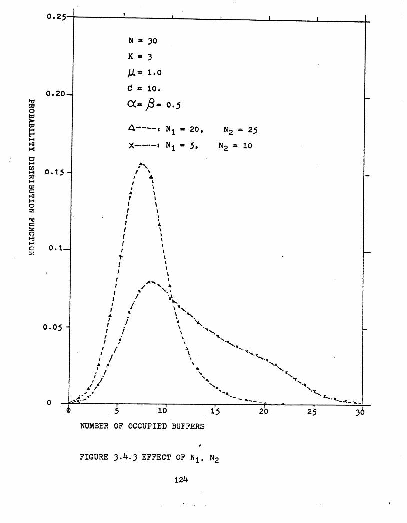
N=30
K=3
_4 = 1.0
= 10.0.20
,8 -=,'_ C_= =050t:_
'=' _, .... , N1 = 20,"4 N2 = 25t"I-4
X .... = N 1 = 5, N2 = 10i-¢
0.1=; t-- -" ,I,' A
I-4 l &Im w %C: A %l-Y r LI-I
Z r %
c O. l _
f
e / %_%.r ,
' i ', ',,tO.05 r / _ "'%.
P / A '%.I % "(_.I / % '¢"_._, "
I i _ _,.% _%,%,/ i "_
/ z" • "_"k
J I _'"4, "'(_,
Z" ".._ "]L_._tt"-,.al...)_..
._ 14 _'_ 25 2_ 3NUMBER OF OCCUPIED BUFFERS
r
FIGURE 3.4.3 EFFECT OF N1, N2
124
I

0.25 I .J .. _ t r ;I
N=30 !I
Kffi3 I!
_- 1.o lio.2o- 1o.
w EXffi = 0.5 I
I.'4
'&,--'-- 8 N1 = 20, N2 ffi 25
X .... I N 1 ffi .5, N2 = I0. _I-e " I,
= o.I_- _i -I-IIm ,f-
IIt-3I-,4 1"o _ ,Al
O I?
0
/i= 0.10-
//;/
t/
,/
;?o.o5- _/ -
t-,&
/t
t
,llLg w"
0 I _r'x"'"_'_--"_"; _ i-'am'a_''4w*=
Q 5 10 15 20 25 30
NUMBER OF OCCUPIED BUFFERS
f
FIGURE 3.4.4 EFFECT OF N L, N2 IN HEAVY LOAD CONDITION
125
• L

0
0.2 0 06 08 10TRANSFER RATE OF DISk ((_)_)
FIGURE 3.4.5 EFFECT OF DIFFERENT DISK RATE
126

4
I ! I !
N=30
N t =10, N2 =20, K =3".,Dq
i= 1o. # = 1.o. c<- 0.5. /3-0.5.0=10. o
i] . .
0.08 ....... s --r----_'_onen_-_lTransfer Time.,0
_ ...... I Erlang Distribution with Degree 10.
o.od - I-------_. -
• t •
0.0, ,,,,, . _
!/ :, "-\0.02 , I .
0 .... "_" "" .................... _c _ _d _ 2d 25 3d
NUMBER OF OCCUPIED BUFFERS (I)
f
FIGURE 3.4.6 EFFECT OF ERLANG DISTRIBUTION TRANSFER TIME
127

3.5. Conclusion
Both first-fit alsorithm and dynamic assi6nment of fixed-size buffers sacrifice
the lars;er size packets too much in a heavily loaded system. But both give a superior
memory manal_ement than other schemes in a liEhtly loaded system. The proper choice
of a manas;ement schemes depends on the real environment of the communication
network. Also the priority system discussed in section 3.2 is su68;ested. A small
sacrifice of the low priority job can decrease greatly the blocking probability, and
shorten the response time of hil_h priority jobs. For uniformly distributed packet size,
the choice of the buffer size is not critical, while the method of distributin6 the
memory amon6 different size buffers is important. A secondary storaEe device miEht
well be worth the trouble. Even a relatively slow disk can improve the network
performance, especially if there is a hiEh probability that integrated switch will enter
the overloaded states.
128

!
CHAPTER 4 SENET Network Design..
4.1. Introduction
The special frame structure of the SENET network brings up the two speciali
problems: the channel capacity assignment problem(CA) and the frame skew assignment
problem (FA). The CA problem is solved once and for all for other communication
networks at the time of their design stage. However, the SENET network will
dynamically assiB;n the channel capacity to data traffic under different loading of voice
traffic, and therefore the CA problem also has to be solved dynamically. The FA
problem exists only for the special frame structure of the SENET network. As
mentioned in Chapter 3, the information contained in a frame can only be processed
after the whole frame is received accurately, and no information in a frame can be
changed once the switch has begun transmitting the frame. Different frame skew
assignments may differ by from several milliseconds to one frame period at one
switchin 8 node. This delay is essential for the voice slots which have to pass several
nodes from source to destination.
In Section 2, F_,eneral design variables, performance measures and a formulation
of the problem of designing a $ENET computer-communication network are stated. In
Section 3, the capacity assignment problem is viewed with the small frame assumption.
It becomes the general assignment problem that [Ger73] among, others has solved.
Then the coordinate descent method and Newton's method are used to solve tl4e
general case. A simple example is also given showing, the capacity assip_,nments of
different criteria and constraints. In Section 4, the skew assignment problem is solved
129

as a M]LP( Mixed Integer Linear Problem). in Section 5, a heuristic alBorithm is B;iven
for the skew assignment problem and the results are compared with those of Section
4.
13o

4.2. The Mode!
There will be three sub-sections: variables, performance criteria, and the
formulations of the problem.
4.2.1. Variables
Here we list the variables that are to be considered in this chapter. The list is
by no means complete and a more sophisticated design might involve additional
variables( such as: reliability, priority for voice and data, etc.)
ToDolo_.y: We consider a directed network [N:A]_ where N is the set of nodes( of
cardinality n), and A is the set of directed arcs( of cardinatity m). We shall use
Ni to indicate the ith node and Aij to indicate the directed arc from Ni to Nj. For
convenience of notation, we also index the links as directed arcs with subscript
to refer to the jth link as Aj, and index the node Nij as the node at which the ith
' link is connected to jth link. Sets IN:A] are the topology of the communication
network and are assumed to be fixed over the whole chapter.
Channels: To each link is assigned a capacity ci which is the bandwidth for data traffic_
such capacity will be only considered as a continuous variable. Also, for a given
link i there is a cost Di associated with value of capacity:
Di = di(ci) 4.2.1
Which may be the real cost of the links or just a reflection of voice loading on
the link. For the linear cost situation we will use d as the cost vector, in which
di, the ith element of d, is the capacity-cost of ith link.
Traffic Matrix: Let Xij [packets/sec] be the required average rate of transmission of
t
131

dat.a packets from link i to link j. If link i is not directly connected to link j then
Xij=O. XO,j is the traffic 8;enerated by the node where link j begins. Xio is the
traffic destined for the node where link i ends. The routing policy of the packet
is not considered here.
The channel flow X.j is the traffic on link j.m m
x.j = i=o:_:'x'iJ = T't. x.ji 4.2.2i=o
Let I/# [bits/packet] be the average packet size. X.j has to be less than c j# for
all the links, otherwise the queue length of link j will be infinite.
The throughput X, of the whole network is defined as the summation of all
channel flow.m m m
x. = _';k i = ,_ _ 4.2,3i=1 i=lj=O XiJ
Frame Skew: Let sj be the frame skew of link j. sj is defined to be greater than or
equal to zero and less than F, the frame period. All the frame skews are
relative to each other, so there is one degree of freedom of skew assignment.
Usually we set sl=O , which means the first link is the standard link. The skew
assignment will only affect the delay of traffic being transferred tt will not affect
the traffic when It is first generated and when it ends at the node.
Other variables: The storage available in the node could also be considered as a design
variable and associated with a cost. However, in this chapter no such
consideration is made.
Priority can be assigned to packets according to their nature (acknowledgement,
control packet intrinsic priority, etc.) or weighed by their length. The possibility of
dividing the packet inlo priority classes( wilh the number of classes and boundaries as
desig;n variables) would probably affect the design of the network; however, we do not
consider such a feature and assume that atl queues are managed on a FIFO basis.
132

4.2.2. Performance Measures
Several criteria can be adopted to measure the performance of a communication
network. The lists here are the performance measures most commonly used.
AveraF.e Message Delay Te
Recall, from [Kle70], that the general expression of the message delay T is of
the following form:
1 m m
T = Ej_=I i=_o_,ij[Tij(si,sj,Pi,nij),Pi] 4.2.4
where _. = the total throuF_,hput [packets/sec]
si = frame skew of ith link.
Pi = propagation delay in link i [sec/messg]
nij - processing time in the node connecting link i to link j.
Tij = delay on the node connecting link i to link j [sec/packets].
Tij consists of the node processing time, queueing time for link j and the waiting
for the frame to be transmitted. For the special frame structure of the system, Tij has
the following form:
Tij = sij+rij(sij)-F for i#O 4.2.5
where sij is the mis-matched delay of link j from link i.
sij = sj-(si+Pi+nij) mod F
is the time left for data packets to be transmitted after they have arrived at the
node and had the necessary processing.
Because the number of frames is a non-negative integer random number
dependin 8 on sij , rij is the number of frames the data packet has to wait until it is
1:}3

transmitted. For Xoj traffic, Soj is assumed to be uniformly distributed in the interval
[O,F) and rij is half a frame period.
A queue for link j is formed. The input is a joint of streams x.ij for all i, each of
the streams comes in at the discrete time -sij+k.F for all intesers k. The averase Tij
becomes
430
Tij - s..+_ Prob[(k-t)-F < W-sij < k-F]-kF 4.2.6U k=O
where W is the waiting time at the queue of link j.
In this chapter, we will make the followin8 assumptions in different situation.
(i) Independent Assumption" We are using the assumption made by
Kleinrock[Kle72] that the independence between the arrival time and the len_;th of a
data packet can be interpreted as that the packet enters the network from an external
source. With exponentially distributed packet len6th and no acknowledsement traffic
[Kle70], the queue is modeled as a M/M/[ system.
Prob[rij(sij) = k] = Prob[(k-t).F <_W-sij <k.F] 4.2.7
= ,,_kF+sij dF(W) 4.2.8(k-1)g+sij
where
dF(W) = (_¢j-X,j)exp[--(pcj-x.j)W] dW 4.2.9e
So(3O
rij = _' k-Prob[(k-1)-F < W-sij < k-F]k=l
OO
= _ k.exp{-[(k-1)F+sij](pcj-Xj) } - k.exp{-(kg+sij)(pcj-Xj) }k=t
CO
=exp[-(pcj-Xj)sij]E 1exp[-k(pcj-Xj)F]
exp[-{pcj-Xj)sij]= 4.2.10
i-exp[-(pcj-X.j)g]
13 +

Tij = sij+rij'F i_O 4.2.1 1
for
roj =, F/2 + F/(,ucj-Xj) 4.2.12
(ii) Deterministic Assumption. The packet size and the traffic flow are
deterministic. The voice slots can be considered as a deterministic packet flow in the
network. This is also the limiting case that the frame period is large compared to the
mean service time of a link for a data packet. By the law of large numbers, the
standard deviation of the summation of n independent random numbers is only 1/n of
each of the individuals. In the frame structure, all the packets coming in a.frame. ,
period are packed and transmitted together. The variance of waiting time decreases
as the frame size increases, and rij>O is nep_,ligblecompared to sij. We have
Tij = sij.
Mean-kth-P0wer Delay T(k)
in the paper [Mei72] it was observed that, in minimizing T, a wide variation was
allowed among the delays Tij. In order to take into account such variation, the
following alternative performance measure was proposed'm m
1 _ _ T_ ]l/k 4.2.13T(k)= [ _" j=l i=0 X'iJ
where kZl. If k is large enough, the variation among packet delays is
considerably reduced at the expense of a higher average delay. [Mei72]
t35
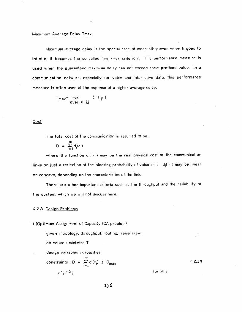
Maximum Avera_,e Delay TmAx
Maximum average delay is the special case of mean-kth-power when k goes to
infinite, it becomes the so called "mini-max criterion". This performance measure is
used when the F=uaranteed maximum delay can not exceed some prefixed value. ]n a
communication network, especially for voice and interactive data, this performance
measure is often used at the expense of a hip,her average delay.
Tmax = max { Tiji }over all i,j
Cost
The total cost of the communication is assumed to be:m
D = ",_ di(c i)i=1
where the function di( • ) may be the real physical cost of the communication
links or just a reflection of the blocking probability of voice calls, di(, ) may be linear
or concave, depending on the characteristics of the link.
There are other important criteria such as the throughput and the reliability of
the system, which we will not discuss here.
4.2.3. DesiF,n Problems
(i)Optimum Assi6nment of Capacity (CA problem)
given : topolo_;y, throughput, routing, frame skew
objective : minimize T
desip=,n variables : capacities.m
= '_ di(ci) < Dmax 4.2.14constraints :D i=1 -
jucj >_.Xj for atlj
136

(ii)Optimum AssiEnment of Frame Skew (SA problem)
given : topology, throughput, roulingt capacity
objective :minimize T
design variables : frame skew.
constraints : #cj > Xj for all j 4.2.15
137

4.3. Capacity AssiF_nment Problem
given : topologyp thruput, routing, frame skew
minimize T
design variables : capacities.m
constraints : D = i=1_" di(ci) -< Dmax 4.3.1
.cj z xj
The independent assumption of [Kle72] is used. Tij is assumed as follows:
exp[-(#cj-Xj)sij]Tij = sij + ,F 4.3.2
1-exp[-(_cj-Xj)F]
where sij = sj-(si+Pi+nij) rood F, and 0_<sij<F
4.3.1. Small Frame Capacity Assi6nment
Here the CA problem is solved for the small frame assumption. At the end of
this section we will explain the physical meaning of this assumption. It will be clear
then that this assumption may apply to some systems whose the frame sizes are not
small.
The small frame assumption is that the (#cj-X.j)F is very small, all the nonlinear
term of the Taylor Series Expansion of equation (4.3.2) are neglected.
1-[jucj-X.j]sijTij = sij + .F
[_ucj-X.j]F
!= sij + si
= 1 4.3.3
This is a well-known formula for ordinary con_nmnication networks [Kle72]. Each
138

411
link is modeled as a M/M/1 queue with exponential service time and Poisson inpul.
The service rate of a link is cj [bits/see] and the input rate of data packets is Xj
[packets/sec]. The average packet length is 1/p [bitspackets] and the average
waiting time is pTij [seconds per packet].
The problem becomes:
given : topology IN:A], data traffic routing ;kij, and frame skew assignment sij.
minimize : T =1 -. _' Xj.[ ]kll/k 4.3.4over ¢ X j=t
m
subject to : _ di(c i) S Dmaxi=1
_cj>_x,j for all j
This is the general mean-kth-power delay criterion [Mei72].
For the monotonic property of function x l/k, to minimizin6 x k is equivalent to
minimizing x under the same set of constraints. So the problem can be written as:
I m 1 k
minimize : T = _- J='_IX.;[_],_pcr,,,_ 4.3.5over c
m
subject to: _' di(c i) < Dmaxi=1
pcj>_.x,j for atlj
First the linear cost-capacity function is considered. The objective function is
convex because it is a sum of convex terms and the set of possible ¢ is also convexj
therefore a local minimum is also a global minimum [Had64]. This problem can be
solved usin8; the LagranF=e Multiplier.
The Lagrangian L for the problem is
L = T+_(D-Dma x) 4.3.6
' = X" I [_ + _( djcj-Dmax) 4.3.7_cj-Xj 1
where /_ is the Lagrangian multiplier.
Z39

• By differentiating the equation wilh respect to cj, we obtain
-- L -- ...__J["._....___.](k-1).' "' + /_dj 4.3.8c3cj >, pcj-Xj (pcj-X)j _"
By setting the parlial derivative to zero we obtain the optimum expression for cj
pcj = ;kj + _.(Xj/dj) l/(k+l) 4.3.9
where o,'_is a parameter independent of j. Compuling _ by satisfying the cost
constraint obtain:m m
,_ = (Dma,,-_ djXj)/[j_ 1 (Xj/dj)l/(k+])] 4.3.10"j=l =
This expression of pcj is first derived by [Mei72]. When k=l, the problem is to
minimize the average delay of the network, and the optimum assignment of cj is so
called "square root" assignment [Kle72]. For the rain-max criterion, k--,oo, cj evenly
distributes the residue capacity (Dmax-_' djXj).
pc! °°) = Xj + _(o_) = Xj + (Dmax-_ dj;kj)/m 4.3.11J
Concave Cost-Capacity Function
For the concave cost-capacity function, the algorithm to find the local minimum
can be constructed similarly to the algorithm developed by [Ger73] which solved the
special case of k=l. No algorithm to find the global minimum existed. The algorithm
follows, the detailed proof of existence and convergence is cited in [Fra72] and
[Get73].
Let us assume that di(c i) is a concave, nondecreasin£, function of ci, for
i--1, 2, 3,.,. , N. (see Figure 4.3.1)
140

d
t"
.I
FIGURE 4.3.1CONCAVE NONDECREASING COST FUNCTION
The inspection of the cost constraint of equation (4.3.1) shows that the set of
feasible ci's is not convex. Therefore, there exist in general, several local minima. If
we assume that all functions di(ci) are continuous and differentiabte for ci>f i, then the
local minimum is characterized by the following properties:
Properfy 4.1
If c is a local minimum for the concave problem, lhen it is also a global minimum
for the problem with cost-capacity curves linearized around c. (see Figure 4.3.2)
_
Cr
FIGURE 4.3.2 LOCAL MINIMUM
The above property is an immediate consequence of the fact that the set of
feasible moves c_caround c is the same for both concave and linearized problems.
Prqperty 4_.2
If c (n) is a feasible assignment, and c(n+l) is the solution of the problem
tinearized around c(n), then
T(c(n+l)) _< T(c(n)) 4.3.12
1_1
Dconcave(c(n+l)) <__Dlinear(c(n+l) ) < Dmax 4.3.13
where Dconcave(c(n+t))is the cost computed on the concave curves and
Dlinear(C (n+t)) is the cost computed on the linearized curves of c(n).
Property (4.1) and (4.2)lead to the following algorithm for the determination of
local minima.
AIAorithm 4.1 Let c(0) be a starting: feasible assignment.
[0] (initial) Let n=O, To=OO
[].] Compute c(n+l)=solution of the problem linearized around c(n) and compute
Tn+ t--T(c(n+l)).
[2] If ITn+t-Tnl<_:, where { is a proper positive tolerance, stop; c(n+l) is a local
minimum within the tolerance, otherwise, let n=n+l and go to [1].
There is an important case of the concave cost-capacity funtion in which the
local minimum is unique and coincides with the g;Iobal minimum. Such a case is known
as the "power law cost function" [Kie70] and the cost function is given by:
di(ci) = diciO_ + dio 4.3.14
where 0<6_<1
The "power law cost" case has been discussed extensively by Kleinrock and a
proof of uniqueness of the local minima can be found be in [Kle70].
Now we will discuss the physical meaning of the small frame assumption. The
first order Taylor series expansion will be a good approximation if (I-X.j/#cj);ucjF is
small for all j. There are two situations for which this condition will hold. One is when
,ucjF is very small which is why we call it the small frame assumption, cijF, which is the
number of bits for data traffic durinp:, a frame period is small. This situation may occur
on a slow speed link sub-network or on a network with heavily loaded voic:e traffic

that little capacity is left for data traffic. The other possibility is when (1-;kj/pcj) is
small for all j. This is a heavily loaded network for data traffic. The average queue
length of links is relatively large and the nature of the frame structure loses its
property of discreterness.
If either of the above situations happens, the small frame assumption applies and
the network becomes the ordinary packet switching communication network.
4.3.2. General Capacity AssiKnment
The small frame condition is dropped here. First the linear cost-capacity
condition is considered. We have the problem
given : sij, Xij, di.
m m Xij exp[-(pcJ-;kj)sij] ]kminimize : T = 2_' _' m [ 4.3.15
over c j=l i=O X 1-exp[-(#cj-Xj)F]
subject to : ¢j>_Xjm i
j_=l djcj<-Dmax
The objective T is also convex because it is a sum of convex terms and the set
of feasible c's is convex, therefore a local minimum is also a global minimum [Had64].
We first ignore the constraint pcj>;kj and verify that the solution satisfies it a
posteriori. We also notice that the optimum solution satisfies the cost constraints a_t
equality and therefore regard it as an equality constraint. Now tile problem becomes:
minimize T(c) 4.3.16over c
m
subject to j_=l djcj = Dmax
|nstead of minimizing the above problem, the following unconstrained problem is
minimized.m
minimize f(cl/3)=T(c)+/_(j_1= djcj-Dmax )2 q.3.1 ;7
1#3

Let {_h}, h=l,2,..-., be a sequence tending to infinity such that for each h, /3h>O
and _h+l>/Sh . Then for each h solve the problem : minimizing, f(clf_h) and obtaining a
optimum solution c(h). By the theorem of section 12.1 of [Lue73] we know that any
limit point of {c (h)} is a solution of the orip_in problem. Because the local minimum is
also a global minimum there is only one limit point of {e(h)}. And for each h such thatm
_' djc(j h)j-1 ,, Dmax, then c(h)=e.(h+l) and therefore the optimum solution has been
found. The algorithm is as followed:
Algorithm 4.2
[0] (initial) set n=O, solve for f(cl/:'to) by some global convergence algorithm.
m d c(h) c(h)[1] If j_=l j j =Dmax, stop; is the optimal solution, otherwise _h+l=_/_h •
[2] Solve for f(c(h+l)l/_h+ 1) by some fast locally convergent algorithm, go to [t].
If we choose too large a /30 to begin with, the initial solution wilt conver_,e very
slowly, while too small a /% will result in a lot of iterations. Here we propose two
different algorithms for [0] and [2]. For h=0 the property of 61obai convergence is
very important, we have to find some thinp= to begin with. The Coordinate Descent
Method is chosen for its well-known global convergence property. But for h>O, the
approximate solution is known, so the local convergence rate is the criterion with
which to choose the algorithm. Newton's method for m-dimension is chosen. Newton's
method has convergence rate 2 but has to inverse a matrix of dimension m. In this
case, there exists a neat analylic form so that the inverse is quickly obtained, and we
have a very fast algorithm.
Coordinate Descent Methods
Instead of solving the m dimension problem at once, we solve the problem one
dimension at a time.
144,

minimize f(cl,c2,..c m) 4.3.18over cj
The cyclic coordinale descent algorithm minimizes f cyclically with respect to the
coordinate variables. Thus c! is changed first, then c2, and so forth through cm. The
process is then repeated starting wi|h c| ag_ain. AlthouEh no proof can be given for
the global convergence of Newton's method. Newton's method of one dimension for
this problem can be proven to be globally converge. For coordinate c j, fj(cj) is thei!
objec! function. Because fj(cj)is convex, fj (cj)<O, the local minimum is also the _lobal
minimum and there is at most one local minimum point, fj(cj)is continuous and its first
derivative is also continuous for all jucj>Xj, fj(cj) is negative at ,cj=Xj and positive at
cj=oo, so the stationary point, fj'(cj)=0, exists. Because of its convex property, fj(cj)
has a local minimum. In the second derivative of f j(cj) with respect to cj every term is
positive and is a monotonic decreasing function of cj. It is easy to prove that
Newton's method is globally and locally convergent for such a function. The iterative
formula is as follows:
c(n+1),..c (n)-. . fj'(c(j n) )/fj"(c(j n) ) 4.3.19J J
By the theorem of the coordinate descent method, if every coordinate is globally
convergent then the whole problem is also globally convergent.m
Newton's Method
Newton's method for m-dimension has a local convergent rate of 2, althouB;h it
may not be globally convergent. For this problem, it does diverge at points far away
from the optimum points. The order of convergence is defined as the supremum of the
non-negative numbers p satisfying

Irn+ t-r*l0<_limit <co 4.3.20
n--)co Irn-r*lP
for sequence {rn} converge to r*.
Before explaining the algorithm, let us introduce some notation: For a scalar
function f(c) of vector c, the gradient of f(c), Vf(c), is a vector whose ith element is the
partial derivative of f(c) with respect to cj. The Hessian matrix, I;'(c), is defined with
the (i,j) element as the secondary partial derivative of f(c) with respect to ci and cj.
The iterative formula of Newton's method of m-dimension is
c(n+l) = c(n)_ [F(c(n))]-lVf(c(n)) 4.3.21
f(c) is the f(cI:_) of equation (4,3.17), it is easy to see that f(c) has second partial
derivatives. If c is near the minimum point, I"(c)is positive definite and the method is
well defined. Now we will prove that F(c) is positive definite for every point. F(c) has
a very good property that it can be represented as a diagonal matrix C(c) plus 2,4_|ci'
Where Ct(c), the (i,i)th element of the diagonal matrix C(c), is equal to the second
derivative of T(c) with respect to ci and is greater than zero for all ci,
F(c) = G(c)+2flkdd'. 4.3.22
where tl is the cost-capacity vector, and d' is its transpose. By definition of
positive definite.
x'F(c)x = x'G(c)x + 2flh(X'd)2m
= _ xj2Cj(c) + 2flk(X'd) 2aj=l
>_.0 for all c 4.3.23
The equality holds only for x=O, by the definition that F(c)is positive definite for
all c. Because F(c) can be represent by this form, l;'(c) can be inversed very easily.-
IF(c)] -1 = [G(c) * 24hd,l'] -1
= G-l(c)[] • 24hG-l(c)dci'] -1
1/.I.6

= C_,-l (c)[] - 2/thG- l (r.)dd'/(l .2flhd'C - l(c)d)] 4.3.24
Here we use the identity formulaI
[I .×y']-I = I-_ 4.3.25l,x 7
Concave cost-capacity condition
m
The constraint is now i=Z_ldi(ci)-<-Dmax,and the unconstrained optimum problem
becomes:
111
j_= dj(cj)-Dmax )2 4.3.26minimize f(cl/th) = T(c)+flh( 1over c
The Hessian matrix now has a more complicated second term. Let ])(e) be the
second term of F(c). Then the (i,j)th element of D(c), the second derivative ofIll
[j'_"=l dj(cj)-Dmax]2 with respect to ci and cj, is as fotiows:
d d
Dij(c) = 2 [---;---di(ci)]'[ ,--t----di(ci)] 4.3.27ac i acj ' •
d d 2 m
Dii(¢) = 2[.._r.__i(ci)]2+2 di(ci) [ _ dq(cq)-Dmax] 4,3.28dci • dci2 q=l
' D can be presented by a diagonal matrix TdVd', where Vd is the gradient of d,,
with ith element di'(ci). The Hessian matrix F(c) of equation (4.3.21) becomes:
F(c) = O(c) + D(c)m
j_ dj(cj)-Dmax] 4.3.29= C(c) + 2flh\TdVd" + 2flhH(¢)[ =t
where the diagonal matrix H(c) has ith element di"(ci), the second derivative of di(c i)i
with respect to ci. Now the positive definite properly of I,'(c) may not be valid. The
choice of /_h must be made very carefully. In the begining, /3h is chosen very small ._om
that Gi-2flh[_ dj(cj)-Dmax]Hi is always positive. Then the /_h can be larger but• ' j=l
always keep /_h[_ di(ci)-Dmax] very small so that the Hessian matrix is positive
definite around c(n), the nth iterative value,
148

,,d
4.4. Frame Skew AssiKnment Problem
In this section the problem of the skew assil_nment of SENET network is studied
in order to minimize the data packet delay throush the network.
4,4.1. Formulation
The capacity assignment problem has the very good property that both the
objective and the constraints are separable functions( i.e. expressed by summations of
terms, each term representing the constitution of an individual link). Unfortunately, the
frame skew assignment problems do not have such good properlies. Another problem
is that the skew time is a rood function which is neither linear nor cone.ave. To solve
the FA problem is very difficult, so only the deterministic model is tried (i.e. the
deterministic assumption in section (4.2), in which the service times of packets are not
random variables).
The problem is
given : Pi, nij, Xij
minimize .._ X.ij{[sj-(si+Pi+nij)]mod F} 4.4.1over s ij
subject to : O_si<F for all i
To simplify the terms without loss of 6enerality, we will use nij to present the
terms (Pi+nij) rood Fo The propagation delay Pi on link i is absorbed in nij , the
processing time for transfer traffic from link i to link j. The problem becomes
minimize ._ - (si+nij)]mod F} 4.4.2over _ aj Xij{[sJ
The non-linear rood function is replaced by the followin8 form.
zij = sj - (si+nij)mod F = sj - (si+nij) + kij'F
•
where kij is an integer. If we define zij,si, and nij as beins; in the ran6e tO,F) then kij
can only be one of three values 0, 1, 2. The above non-linear non-concave
optimization problem can be formulized as a mixed integer linear pro6ram as follows:
minimize .._ Xijzij 4.4.3over s _J
subject to 0_<si<F for atli
0_<zij<F for all i,j
" zij=sj - (si+nij) + kijF
kij=0, t, 2o
The above formulation can be simplified. 0nly the zij>0 constraints of zij are
effective. Therefore the slack variables zij can be eliminated and the problem becomes =
minimize _' -(s i F] 4.4.4over s ij ;kij[sj .nij).kij
subject to. O_<si<F for all i
sj-(si+nij)+kijF>O
kij=O,.1.,2 forl all i,j.
It seems that the constraint that kij be a non-nes;ative integer no F,reater than 2
is also unnecessary. However in the state of the art, the al6orithms to solve inte_,er
prosrammin8 are not very well-developed and the upper limit constraints of kij do
prevent the alF.,orithm from drifting away.
4.4.2. Branch and Bound AIp,orithm
Branch and bound al6orithm , an optimization technique that uses the basic tree
enumeration, is used to solve the above M]LP( mixed inte_;er linear pro6ram) [Gar72,
Lan73]. A binary tree is formed with each ed6e imposin6 a constraint and each vertext
1.50

j representing the set of constraines given by the edges along the unique path Pj from
vo to vj.
.. / "
FIGURE 4.4.1 _]RANCH AND BOUND TREE ENNUMERATJON
If no further exploration from a vertex can be profitable, it is said to be
fathomed. More generally, if the problem is to find every x(S, then vertex j restricts x
to Sj, where Sj is the intersection with the set of points satisfying the constraints
given by the edge Pj. If pj has k+t vertices denoted by
vo=vj(o) , vj(t) , ....... Vj(k.1) , Vj(k)=V j 4.4.5
then
S=Sj(o)m Sj(t)= = = ..... =Sj(k)=S j 4.4.6
We call Vj(k_l) the predecessor of vj, which in turn is called a successor of it.,;
predecessor. If a vertex j does not have any more integer constraints, it is called a
tail vertex, or just a _ i.e. all integer variables of the original problem are fixed by
the set of constraints Pj. If the original problem is an all integer program, then the
value of the object function at the tails can be obtained by substituting all the
constraints. |n the M]LP cases, the tails, with all the integer variables fixed, have to
solve a pure linear program to get the object function.
A vertex that is not fathomed and whose corresponding constraint set can be
separated more is called a live vertex. Branc hinp, means choosing a live vertex to
consider next. The rule of branching considered here is to choose one of the
t51

successor vertices of the vertex currently bein_ considered. If the current verlex j is
fathomed, one simply backtracks along Pj until a vertex having at least one livee
successor is found. One of those successor vertices is chosen for branching. If there
are no live vertices, the enumeration is complete.
In a pure enumeration method, every tail is calculated. |n branch and bound
algorithm, every vertex is estimated by an upper bound and the algorithm will go to its
successors only if it is not fathomed, i.e. if there is any possible improvement of the
object value. Let the problem be:
max z(x}, x_S 4.4.7
Suppose the enumeration is at verlex j in the tree. The problem considered at
vj is
max z(x), x{Sj 4.4.8
Let
z(x_'(j}) . if xj _ solves equation (4.4.8).
zj t = { -co if Sj is an empty set. 4.4.9
co if equation (4.4.8) is unbounded.
An upper bound zj>_.zj* may be calculated by considerin6 the relaxation of
equation (4.4.8).
max z(x) x(Tj_Sj 4.4.[0
and letting
co if equation (4.4.10) is unbounded
zj = { -co if Tj is empty, infeasible 4.4.1 t
zj0=z(x0(j)) if x0(j) solves equation (4.4.J0).
The choice of Tj is one of the critical parts of any branch and bound all]orithm.
]t must be chosen such that equation (4.4.10)is relatively easy to solve, but at the
152

®
same time must yield an upper bound at a vertex which is valid for any of its
successors, since, if v k is a successor of vj then Tj_Sj__$ k. Here the choice of Tj is
made as follows: . .. .:....11'
= {x,ylAlJx+A2Y=bJ, x>_0inte_;er, y>_0} _ 4.4.12 ""Sj
= {x,ylAlJx+A2Y=bJ , x,y>0} 4.4.13Tj
so that zj is calculated by sotvin8 the correspondin6 linear pro6ram. The al6orithm to
solve the MILP is as follow=
Let us define BEST=best solution discovered so far satisfyin8 all the discrete
constraints.
AtEorithm 4.3
[O] (initial) BEST=-co.
[1] Set the new vertex as vertex j. Solve the linear program Tj. let
FUNC=value of the object function of this linear prol_ram.
[2] Check the position of vertx j. If it is a tail then go to [3]; otherwise F_-,oto,
[4].
[3] (It is a tail vertex) If the value of the object function FUNC is 8rearer than
BEST then substitute the best solution with vertex j, then 8o to [5].
[4] (It is not a tail vertex) If value of the object function is p..,reater than BEST,
this vertex is live, then 60 to [6]; otherwise this vertex is fathomed, in whicll
case 60 to [5].
[5] (back up) Current vertex is either a tail or fathomed. Backtrackin8 alon6 Pj
until a vertex havin6 at least one live successor is enumerated. Set that live
vertex as the new vertex considered. If there are no live vertices, then
1.53

stop, the enumeration is complete, output BEST and the correspondin8
vertex; otherwise EO to [1].
[6] (branchins) [t is probably profitable to F=o on further. Choose one of the
successor vertices of a current vertex as the new vertex considered, F,o to
C1].
4.4.3. Acceleratin_ AlKorithm
The above is the standard branch and bound algorithm for M]LP. Notice that if a
vertex is infeasible, i.e. zj=-oo, it takes solving a linear program to find out. In the
problem of equa|ion (4.4.4); there are other intrinsic constraints which make a lot of
vertices infeasible. Before we go furlher, some graph theory terminologies are
explained. ]ntuitivly speaking, a dJ-Eraph (directed p=raph)i5 a set of points, and a set
of arrows, with each arrow joining one point to another. The points are called the
nodes of the poraph, and the arrow_ are called the ar(:._._._._of the _raph. An arc is
represented by' an ordered pair (,x,y), where x alld y are vertices of lhe i_raph, node x
is called its initial endpoint, and node y is called its terminal endDoint. Node y is also
called a successor of node x, while node x is predecessor of y. If the directions of the
arrows in a graph are not specified, the p_:,raph is called an undirected _ or just a
Eraph. The arc without any specification of its direction in the undirected graph is
called an ed_,e. An undirected _raph is callled a simpl e _if:
(i) ]t has no edE_e of form (x,×).
(ii) No more than one edge joins any two nodes.
A sub_raph S of a p=raph G is a p=raph with the set of the nodes a subset Of
nodes of G and the set of arcs a subset of |he arcs of (3. A chain is a sequence
15#

q=(ui,u2,., -, ur) of arcs of G such that each arc in the sequence has one endpoint in o
common wilh its predecessor in the sequence and its other endpoint in common with
its successor in the sequence. A" _ is a chain such that the two endpoinls of the
chain are the same node. A _raph is connected if there exists a chain q(x,y) for each
pair (x,y) of distinct nodes. The graph is called separated if it is not connected. A
tre__..e.eis defined to be a connected graph without cycles. Edges in a tree is called
branches.
Now look back at the constraints:
sj-(si+nij)+kijF>_.O for all Xij>0 4.4.14
O<si
For convenience, a delay graph is constructed to show the traffic and the delays
of the real communication network. Let the node of the delay graph be the
communication links, an arc (i,j) on the delay graph exists only if the traffic Xij of the
communication network is non-zero. Figure 4.4.2 shows an example. Then for the
summation of equation (4.4.14) over a cycle L of the delay graph, we will Get:
:_ < :E F for every cycle L 4.4.15(ij)(L nij - (ij)_:L kij'
We will prove that equation (4.4.15)is the necessary and sufficient condition for
equation (4.4.14) to have a feasible solution. Suppose a system of linear inequalities
f i (x)>_._i (l<i<p) 4.4.16
where fl t f2t. t., fp are given linear functionals on xD and _1, c_2_"" '_p are
given real numbers. The system is said to be consistent_ if there exists an x which
satisfies the above system; otherwise it is said to be inconsistent.
Theorem 4.1 (Consistence Theorem of [Fan56] )
A system fi(x)>_,'-i for i=1,2,., .,p, is consistent if and only if every set of positiveP P
numbers Xi satisfies i=:'_lXifi=0 which in turn implies that i=_lXi_.i<0.
1.55

Another way to state this theorem is that if a system fi(xi)_-_.i, (l<_i<_p) isP
inconsistent then there exists a set of positive numbers {Xi} such that i___lXifi=O andP
i=:_--'1Xio,'.i'.zO.
Theorem 4.2
Equation (4.4.14) has a consistent solution for {si} and {kij} if and only if
equation (4.4.15)is satisfied.
Proof : The necessary condition is easy if {si} and {kij } are consistent then equation
(4.4.15) is just the positive linear combination of equation (4.4.14), so equation
(4.4.15) will be consistent.
The sufficient condition can be proven by assuming that there exists a set of
{kij } which satisfies equation (4.4.1,5) by not giving a consistent solution of {si}
for equation (4.4.14). Now equation (4.4.14) is just a function of si, and it is
inconsistent.
sj-si>nij-kijF for all Xij>O 4.4.17
Then by theory 4.1 there exists a positive linear combination of equation
(4.4:17) which makes the left part equal to zero. But this linear positive
combination is over the incident matrix of a graph, so this set forms a cycle.
This is a contradiction because we just assumed that equation (4.4.15) is valid
for every cycle. This proves the theorem. #
AIKorithm 4.4 Check the feasibility of the vertex of M]LP.
[0] (initial) BEST=-oo, find all the simple cycles of the digraph.
[ta] Set all the nonfixed kij equal to their upper bounds, i.e. kij=2. Check all the
simple cycles to see if {kij } is feasible for inequality equation (4.4.17).
[tb] If {kij } is feasible then solve the linear program with {s i} and all the
nonfixed kij; otherwise set FUNC=-co, i.e. declare the vertex to be fathomed.
1.56

,el
o
By the above algorithm, the feasiblity of a simple cycle is always checked first
before solving the linear problem.
The k-tree algorithm for a simple cycle of a digraph is used in step [0] of
algorithm 4.4. [Ber73] The algorithm is based on k-formulas, which are a linear
notation for the specification of digraphs. The notation was introduced by Krider
[Kri64]. The trees of k-formula are called k-trees. Let N={1,2,3,...n} be the set of
nodes of the digraph. Collect the links for all k(ZNfrom which links originate into a tree
with node k the root, and the terminal nodes arranged in ascending order from left to
right. This tree is called the atomic tree of node k and is denoted tk.
/ .2 I o Io 30
z./. FIGURE 4.4.2 ATOMIC TREE
First the atomic trees of all nodes of the digraph are merged into a single k-tree
or a set of k-trees, T1,T2,. ,. ,. ,. ,.Tm. In one k-tree, any specific atomic tree can
appear at most once. Here is an example of forming of a k-tree.
FIGURE 4.4.3 K-TREE
tS?

Note that a k-tree must merge as many a|omic trees as it can, but for some k-
tree it may' not be able to merge every atomic tree of the digraph.
Then we can find all cycles of the di6raph by traversing: the k-lrees and
checking the path from the root of the tree to the terminal node. If the path contains
a subpath (Ck,.,.,.ck) then one cycle is found, By carefully markin8 nodes, the duplicates0
can be eliminated [Ber73].
158

d...,=lk
4.5. Heurintic Algorithm
Even with the accelerating algorithm of section 4.4.3, the mixed integer linear
proBrarn stlll runs very slowly. For a communication network with 4 switchingnodes
and a complete graph topology with duplex links, there are 12 real variables and 24.
integer variables. For a pure enumerating method, 324 ( each integer has three
choices) linear program of 12 variables have to be solved. So inherently the integer
programming costs a lot of computation time. Next we will discuss some properties of
the optimum solution and develope a heuristic algorithm from that.
4.5.1. Cuts and Trees
Here a graph implies a simple connected graph. A maximum .,.,panning tre.._..eeT of a
connected graph G is a tree subgraph with a set of nodes containing every node of G,
Unless otherwise noticed, a tree implies a maximum spanning tree. A cu.....t.tis a set of
arcs in a graph such that if the arcs in the cut are removed from the graph the graph
will be separated. The set of fundamental cu..__trelative to a tree T is the set of
minimum cut such that each cut contains one link in the cotree G-T of T. Where the
minimum cut is a cut such that any strict subset of it is not a cut. A fundamental cut C i
of tree T is a fundamental cut which has branch i of T in it. Arcs in the tree are called
branches while arcs in the coffee are called chords.
Lemma 4.3
Suppose a communication network which has links a, b, c with non-zero transfer
traffic to link r, i.e. Xar, ;kbr, ;kcr greater than zero. And suppose ta, tb, tc are thee
Z.59

times when the transfer traffic has finished being; processed and they are ready to be
sent out. Then the oplimum assi6nment of the frame skew of link r must be equal to
either of t a, t b, or t c. Where optimum assiF:,nment is defined as the assi6nment of the
least total waiting time.
The general form of the total delay at this junction is the sum of [(s r-
t i) rood F],Xir where i = a, b, c.
Suppose that the optimum sr is not equal to any of ta, t b, t c. Without loss of
generality, suppose Sr, the skew assignment of link r, lies between t a and t b.
""'-""'---'_--" ,_ I !
c_ o _;+._. F
FIGURE 4.5.1 MERGING LINK CONFIGURATION
The delay at the junction will be
(Sr-ta)mod F + (Sr-tb)mOd F + (Sr-tc)mOd F
-- (Sr-ta) Xar + (F-tb+s r) Xbr + (F-tc+S r) Xcr
= (Xbr+Xcr)F - (taXar+tbkbr+tckcr) + (kar+Xbr+Xcr)Sr
=, _+(Xar + Xbr+Xcr)-Sr 4.5.1
It is obvious that decreasing sr a little will produce a smaller lotal delay. So it
is a contradiction that s r is the optimum skew assignment. It can be proved similarly
for other configuration of skew assiF_,nment. So for a single network like this the
optimum assignment of link r must be matched to one of the links.
That communication networks with more than three input links merge into one
link can be proved similarly, for the third term becomesk
i___1(F-ti+sr)Xir = (F-tc+Sr)Xcr 4.5.2
with
160
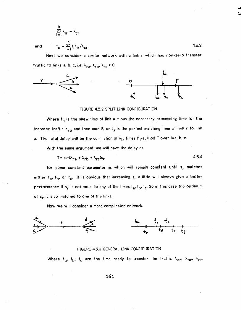
k
i=l;kir = ;kcr
k
and tc = i=:_lliXir/X.cr. 4.5.3
Next we consider a similar network with a link r which has non-zero transfer
traffic to links apbp c_ i.e. X,ra, ;krb , X.rc > O.
FIGURE 4.5.2 SPLIT LINK CONFIGURATION
Where ta is the skew time of link a minus the necessary processing time for the
transfer traffic Xra and then rood F, or ta is the perfect matching time of link r to link
a. The total delay will be the summation of X.iatimes (ti-sr)mod F over i=a, b, c.
With the same argument, we will have the delay as
T= o,.-(Xra + Xrb + Xrc)Sr 4.5.4
for some constant parameter ¢_ which will remain constant until sr matches
either ta, tb, or t c. ]t is obvious that increasing sr a little will always give a better
performance if sr is not equal to any of the times ta, tb, tc. So in this case the optimum
of sr is also matched to one of the links.
Now we will consider a more complicated network.
FIGURE 4.5.3 GENERAL LINK CONFIGURATION
Where t a, t b, t c are the time ready to transfer the traffic Xar, Xbr, Xcr,
161

respectively. And td is the skew time of link d minus the necessary processing; time
for traffic krd. t e,tf are definedslmilarly. In other words, those timest a,t b,t c,t d,t e,
and If are the perfect matching times for link r to the specific links.
Lemma 4.4 The optimum skew assignment for link r can always be set to match
one of the links.
The proof is very similar to lemma 4.3. Suppose there is an optimum assignment
of s r which is not equal to any of the matching points. By similar argument to that of
the proof of Lemma 4.3, the total delay of the network will be of the form
T=o"-+(,X.ar+,X,br +Xcr)Sr-(Xr d+Xre +Xrf)s r
If (Xar+X.br+Xcr) is greater than (Xrd+Xre+Xrf), then decreasing sr a little will
always produce a smaller delay for the network which is a contradiction of s r bein[_
the optimum assignment. Sos r must match one of fhe t i. Otherwise, the increase of s r
will always decrease T by the same argumen. If (X.ar+Xbr+Xcr) is equal to
(Xrd+Xre+Xrf) then we can shift sr without affecting the network performance. So we• . ;,
can always shift s r until one link is matched. This completes the proof. #,
Now we consider a general graph. For any subgraph L of graph N, we will
prove that if N is connected, then there is at least one arc which carries non-zero
transfer traffic between the communication links in L and the communication links in N-
L which is matched, i.e. its transfer delay will be zero. Here the graph is the delay
graph which has the oril_inal communication links as nodes and the non-zero transfer
traffic as arcs between nodes. Each arc on the delay graph has a corresponding
traffic and processing time of the communication network.
162

FIGURE 4.5.4 GENERAL NETWORK CONFIGURATION
The argument is very similar to the argument for the above two lemma. If none
of the arcs is matched, then the tendency to decrease the skew time will be
proportional to all the transfer traffic into L, otherwise, the tendency to increase the
skew time is proportional to the transfer traffic leaving L. If the amount of traffic
going into L is greater than the amount of traffic leaving L, then decrease the skew
time a little for all links of L until one arc is matched. This will always decrease the
total delay. The opposite is true when one increase the skew time a little. So in each
of these situations the optimum assignment of skew time for L must have at least one
matched arc. Therefore the following theory is proven.
Theorem 4.5
For the optimal skew assignment in a delay graph, there exists a connected sub--
graph of the matched arcs.
By this theorem, we will only consider the set of skew assignments which has a
connected sub-graph of matched arcs. In graph theory, a maximum spanning tree of a
connected graph can reach every node, so a maximum spanning tree of matched arcs
can determine all the skew of the nodes, or the communication links of the original
163

network. We will call such a maximum spanning, tree as matched tre.._.eein skew
assi6nment.
By heuristic, it seems that the tree wilh maximum total transfer traffic will be
the matched tree of the optimum skew assignment. But this is not true. The following
example will show the reason and will also explore the complexity of the problem.h
I \ %" j,o" "---._..___...-_EoC6)
FIGURE 4.5.5 AN EXAMPLE
The number on the arcs of the delay graph is the amount of transfer traffic
corresponding; to the arc and the number in parenthesis is the necessary processing
time for the arc. The frame size is 10,
Then the matched tree of maximum transfer traffic and the corresponding skew
assignment is L
FIGURE 4.5.6 MAXIMUM TRANSFER TRAFFIC SKEW ASSIGNMENT
The total mis-matched delay is
Xbd[12-(4+4)] + Xde[11-(2+2) ] = 107f
But the matched tree of tile optimum assiBnment is as follows:
FIGURE 4.5.7 OPTIMUM FRAME SKEW ASSIGNMENT
16l+

The total mis-matched delay is
Xcd[18-(5+7) ] + Xde[ll-(8+2)] = 93.
Why is the first skew assignment not optimum? There are two cycles (abdefa)
and (acdefa). The first skew assignment minimizes the cycle (acdefa), and the second
skew assignment minimizes the cycle (abdefa). The cycle (abdefa) has total processing
time 19, and the cycle (acdefa) has total processing time 23. For a network of frame
size 10, the cycle (abdefa)is much more vulnerable than cycle (acdefa). Hence the
first skew assignment fails.
TO search all the possible trees is infeasible for a moderately complicated
network, the number is Cnm-1 where m is the number of nodes and n is tl_e number
pieces of non-zero transfer traffic. A heuristic algorithm which compares the skew
assignments with matched trees differing by only one arc i_ developed. It is wellI
known in graph theory that the set {xi}u{T-i} is also a tree for any arc xi in Ci. Thus
we can replace branch i by any arc of Ci and still make a tree. If we choose these
trees as matched trees in the skew assignment, then the difference between these
skew assignments will only occur at the arcs in Ci. Therefore the algorithm must
choose the arc in a fundamental cut such that the mis-matched delay in the cut will be
minimum..
4.5.2. The Algorithm
Now consider a matched tree T and its relative skew assignment and a
fundamental cut Ci of T. First we mark the nodes on one side of the cut and assume
the skew assignment of these nodes to remain constant, because assigning of the skew
depends on the direction of the branch. Group all arcs in cut Ci into two sets A and B.
165

|f an arc in the cut is from a marked node to an unmarked node then this arc is in A,
otherwise the arc is in B. If we replace branch i by an arc x in the cut as a matched
arc. Depending on the direction of the arc x, the change of skew in the unmarked
nodes will differ. Define x r the originat mis-matched delay of arc x. If x is in B then
every skew assignment of the unmarked nodes should increase an amount x r
otherwise x is in A and |he skew should decrease x r for all ]he unmarked nodes. For
an arc y in C i that is neither i nor x, there will be some change of mis-matched delay
during the change of the matched tree. Now suppose the new skew increases by x r
for all the unmarked nodes, then if y is in B the mis-matched delay should subtract x r
amount, otherwise the new mis-matched delay should add xr amount. The rood F
should apply to the arithematical operation after the results are found. A decrease of
skew by x r is equivalent to a increase of skew by F-x r.
A!F_orithm 4.4
[0] (initial) Read the frame size, the structure of the delay F,,raph that a two
column vector LINE of L elements is set with arc I from node LINE[1,I] to
node L]NE[2,I]. Set the incident matrix which the ilh row has 1 only at node
LINE[1,I] and LINE[2,I]. Set the processing time of arc j at vector DELAY[J].
• [1] Find a tree and set TREE[J]=1 if arc J is in the tree; otherwise TREE[J]=O.
[2]'(set the skew assi6nment of the node by the tree. Mark'anode If tlieskew-_: ; "'i. '
• is assi6ned.) Set SKEW[[]=O, MARK[t]=I; If MARK[I]=! and MARK[J]=O and
we will mark node J if there is a arc K between I and J.
SKEW[J]--(SKEW[I]+DELAY[K]) rood FRAME if arc K is from ]to J and
SKEW[J]=(SKEW[]]--DELAY[K]) rood FRAME if arc K is from J Io ]. Set
MAI_K[J]= t;
166

[3](find lhe fundamental cut) Inversing the (M-t)X(M-1) square submatrix of the
tree and labeling the corresponding column of INCD, the incident matrix will
become the fundamental cut matrix. For each row i, the set of the column j
such that INCD[],J]=I is a fundamental cut with respect to the column which
is labeled i. Because one row of INCD is redundant, so INCD[M,K] is used as
labeling for all K. Set J=l, and continue [4].
[4](find a tree branch) While INCD[M,J]=O increment J by 1, if J>L then the
algorithm complete, stop; otherwise we have found a tree branch J, Set
MINN'-J, cntinue [5].
[5]Put the cut correspondin_ to branch J into vector COTREE, and the number of
arcs in the cut is NB_ if NB=O, then J=J.l Co to [4]_ if NB=I, then if
LEM[COTREE[1]]<LEM[J] and arc COTREE[].] is not matched, then there will be
profit to switch to the new arc. Set MINN=COTREE[I], go to [11]_ if NB>I
then continue [6].
[6]There is a cut corresponding to the branch J of the tree T, mark all the node
in one side of the cut.
[7]Set MIN,=mis-matched delay with J as branch. Set R=I.
[8]Calculate the total mis-matched delay of the cut with COTREE[R] as the new
matched branch, and set the value ms NEWMIN.
[9]If NEWM]N'-'M]N_ then set M]N,,NEWM|N and MINN,,COTREE[R].
[lO]Set R=R+I. [f R<NB, then we have more arcs to look at, F=Oto [8]; otherwise
all the arcs in the cut have been tried, continue [}.1].
[ll]Check if there is a better choice than J. If M]NN=J, then J is the best in this
cut go to [4]_ otherwise eliminate the column M|NN of the matrix ]NCD, so
167

that only 1 in the column is at row INCD[M,.I] where the branch J is labeled.
Set ]NCD[M,M]NN] equal to this row, and unlabel the column J of ]NCD. The
,, elimination process is the same as in [3] where the set of fundamental cuts_ _....
• is found.
[12]We get a new branch, reassign the unmarked node by increase ing or
decreaseing the same amount XR such that it makes branch M]NN matched.
SetJ-,1,goto [4].
The above is the main frame of the algorithm. Step [3] is to inverse some of the
incident matrix and find the fundamental loop. Every iteration will find a new tree and
increase the performance. There is a finite number of trees, so the algorithm will
terminate. This algorithm will find a matched tree such that it is better than all its
immediate neighborhoods where one arc is different. Thus different initial guesses of
matched trees may result in different sub-optimum configurations of matched trees.
168

CHAPTER 5 Conclusion
This dissertation describes the model, the analysis and the design of a special
integrated voice/data computer communication system. The advantages and the
operation constrains of the integrated switch are thoroughly studied. This dissertation
gives guidances of the expected performance and the potential storage requirement.
This chapter presents interpretations of results and indicates directions for future
research.
5.1. Interpretation of Results
In order to meet certain grade of service for voice calls, the communication
system must have some redundant facility in addition to its traffic requirement. The
idea of the integrated switch SENET communication network is to use these redundant
facilities for data packet communication. In Chapter 2, an integrated switch system of
ten voice channels and of job size ratio 10 and 100 is solved exactly. The exact
solutions are also compared with various approximation methods and with results of
similar queueing models. The rationale of the very long data packet queue for the=
integrated switch is thus concluded by thequeue occasionally entering the overloaded
states for a relatively long period. From the heavy load approximation of queueing
theory, we believe that the cliffusion approximation should be a better approximation
when the scale of the _integrated switch increases and be relatively insensitive to the
distribution of the service requirement. Though the quantitative results of a large
integrated switch with the realistic job size ratio need further investigation, the
169

qualitative results do give a _ood meaningful estimation of the potential problems. The
use of the redundant voice communication facilities for data communication will create
a Ions; queue of data packets and will have slow response for interactive data traffic.
It is thus conceived that to have real time response for interactive data communication,
some link capacities shall be reserved for suchtraffic only. In addition to this_ the
integrated switch needs a much larg,er memory space to queue the data packets than
the conventional data communication process.ors such as ARPA IMP°
Althoug;h the data packet queue of integrated switch is rather Ion6, the number
of buffer needed for the switch to operate efficiently is limited. The queueinp= network
of Section 3.3 models the'buffer life-time and the relationship of throushput and
number of buffers, The concep| of processin6 bound and buffer bound switchin6
processor is developed. In order to minimize the blocking probability for Class I!
packets by lacking of buffer and to maximize the memory utilization, a secondary
storage is suggested and modelled properly. The use of a disk for switchin 8 processor
is rather unconventional', a special reservoir model and a special forward and backward
al6orithm are developed. The block transfer time between disk and core is either
Exponential distributed or Erlang distributed. It is shown that the performance of the
switchin 6 processor with disk is insensitive to the distribution of transfer time. Using
a disk for the switch will decrease the buffer requirement and isolate the overloaded-
switch from infectin 8 its neip_,hboring nodes. However the disk may create some
reliability problems and also may complicate the operations of network. Several
schemes to allocate memory into buffers are also discussed and their performance are
compared with each others. Both first-fit assi6nment scheme and dynamic assig;nment
of fixed-size buffer scheme sacrifice the larger size packets too much in a heavy
170

,al
0
loaded system. However both give superior memory management schemes than other
schemes in a lightly loaded system. A reserve priority buffer assignment scheme i,.;
suggested for communication network with priority on its data packets. High priority
, packets can be allocated more buffers than low priority packets can. A small sacrifice
on the low priority packets can decrease the blocking probability and thus shorten the
response time of high priority packets a lot.
[n order to have real time response to the interactive data communication, some
communication link capacity shall be reserved for Class ]| traffic only. The link
capacity assignment to interactive data is discussed as a grade of service trade-off
between Class ! and Class ][ traffic. The SENET communication network with frame
structure and the concave cost-capacity function is solved by the coordinate descent
method and Newton's method. The capacity assignment problem for the SENET
network is different form other communication networks and the link capacities sl_all
be re-assigned when the traffic situation changes. Another problem related to the
frame structure of SENET is the frame skew assignment problem. Because of thl.=
frame period, the delay of packets is discretely incremented by the frame period. The
mis-matching of the frame skew between links will cause the longer buffer life-time,
thus require larger memory space as well as suffer extra mis-match delay. The frame
skew assignment problem is formulated as a mixed integer linear program. A special
speeding algorithm for the global optimal assignment as well as a heuristic algorithm
for local optimal assignment is developed. This frame skew assignment also needs
dynamically re-assignment when the traffic flow on links changes.
171

5.2. Directions for Future Research
With the changing cost structure of processing power and communication power,
many integrated switch networks will be designed and used. The nature of voice and _.
data (:ommunications are still unclear, and the relationship between them are also left
unexplored. The flow control in an integrated switch network is especially important
to the network performance, while it is totally unknown yet. Possible further studies
are outlined below:
1.With a backbone communication network using; T1 carrier, a 10 millisecond
frame contains 15,440 bits. If half of the capacity can be used by Class I
traffic and each voice slot contains 80 bits, then the integrated switch has 97
Class I channels. For a 2000 bits packet, a T1 carrier can transmit the whole
packet in about 1.3 m'illisecond. Comparing, 1.3 millisecond with the average 3
minutes voice call, we find that the realistic Class I/Class I] job size ratio is in
the order of 100,000. An integrated switch of suctl order can be solved by
diffLmion approximation, but the validation of such approximation either by
simulation or other methods still needs lots of efforts.
2.The control protocol for the integrated switch communication network
especially with disks needs a lot of work to find the impact of the present
protocol and the effectiveness of the disk. The feasibility of usin 8 CCD or
magnetic bubble as a secondary storage device and their corresponding models
will lead the communication processor into a better cost-performance region.
172

3.The processing of data packets is assumed to be Exponential distributed. A
simulation for general processing time will give a better understanding of
buffer life-time behavior and mil];ht suggest a better buffer management
scheme.
4.The cost-capacity function discussed in Chapter 4 is assumed to be link,
independent. However, there are some relationship between the cost of
adjacent links especially in $ENET the cost function is the grade of service of
Class I traffic. A study of this will give a more clear picture of data flow in the
network and can provide design guidance of flow control and network protocol.
173

BIBLIOGRAPHY
[ADC75] /ld_,a.ced Data Carnmttnication Control Procedures (/JDCCP),Indeptmdent Nu.mherinff. Proposed American National Standard° FourthDraft, August 1975.
land72] Anderson, R. R., J..F. Flayes, and D. N. Sherman "Simulated Performance ofa Ring-Switched Data Network." IEEE Trans. on Communications, 1972.
tArt61] Avi-ltzhak, B. and P. Naor "On a problem of Preemptive Priority Queueing."Operations Research Vol. 9, 1961.
[Bar76] Barbacci, M. R. and J. D. Oakley "The Integration of°Circuit and PacketSwitching Networks Toward a SENNET Implementation." The 15th NBS-ACM Annual Technique Symposium, 1976.
[Bas75] Baskett, F. et al. "Open, Close, and Mixed Networks of Queues withDifferent Class of Customers." JACM Vol. 22, 1975
[Ber73] Bertiss, A. T. "A K-tree Algorithm for Simple Cycles of a Directed Graph."Technical Report 73-6 Dept. of Computer Science, University ofPiltsburgh. 1973.
[Bha75] Bhat, U. N. and M. J. Fischer " Multichannel QueueinF, System withHeterogeneous Classes of Arrivals." Defence Communication EngineeringCenter CP-75010, 1975.
[Bro68] Brash, I. "Preemptive Priorily Assignment in Multichannei System."Operations Research Voi. 16, 1968.
[Buz73] Buzen, P. " Computational Algorithm for Closed Queueing Network withExponential Servers." CACM Vol. 16, 1973.
[Can72] Cantor, D. and M. Gerla "The Optimal Routing of Messages in a ComputerNetwork via Mathematical Programming:." IEEE Computer ConferenceProceedings, pp. 167-170, San Francisco, Calif., September 1972.
[CMU75] Carnegie-Mellon University "The Application of Multiple ProcessorComputer Systems to Digital Communications Networks." CMU ProposalNo. O8103A to Defense Communications Engineering Center, Defense
Communications Agency, May 1975.
[Cha43] Chandrasekhar, S. "Stochastic problem in Physics and Astronomy." Rev.Mad. Phy. 15, 1943.
[Cha72B] Chandy, K.M. and R.A. Russel "The Design of Mullipoint Linkages in aTeleprocessing Tree Network." ]EEE Trans. on Computers, C-21, pp. 1060-1066, 1972.
174

[Cha75A] Chandy, K. M., U. Herzog, and L. Woo " Parametric Analysis of Queuein8Networks." IBM. J. Res. Develop. 1975.
[Cha74] Chang, A. and S. S. Lavenberg "Work Rates in Closed Queueing Network, s•with General Independent Server." Operations Research, Vol. 22, pp. 838,
1974.• ,,=. •
[Cha75B] Chandy, K. M., U. Herzog, and L. Woo" Approximation Analysis of GeneralQueueing Network." IBM. J. Res. Develop. 1975.
[Cha72a] Chang, J. H. " Some Design and Evaluation Techniques of DataCommunication Systems." iBM. Research Report RC-3736, 1972.
[Chu69] Chu, W. W. "A Study of Asynchronous Time-+Division Multiplexing for Time--Sharing Computer Systems." FJCC. Vol.35, pp. 669, 1969.
[Chu72] Chu, W. W. and A. G. Konhein " In the Analysis and Modeling of a Class ofComputer Communication Systems." IBM. Res. Report RC-3727, 1972.
r.c1o73] Closs, F. "Pakcet Arrival and Buffer Statistics in a Packet Switchin G Node."Data Network Analysis and Design, DATACOMM 73, 3rd data communicationSymposium.
[Cob54] Cobham, A. "Priority Assignemtn in Waiting Line Problem." OperationsResearch Vol. 2, 1954.
ECol71] Cole, G. D. "Performance Measurements on ARPA Computer Network."Proceedings of Second ACM IEEE Symposium on Problems in theOptimization of Data Communication Systems, Pale Alto Calif. Octobel"1971.
[Cov75]. Coviello G. J. and P. A. Vena "Integration of Circuit/Packet Swilching in aSENET (Slotted Envelope NETwork) Concept." National TelecommunicationsConference (NTC), New Orleans, December t975.
ECox55] ' Cox, D. R. "A use of Complex Probabilities in the Theory of StochasticProcess." Prec. Cambridge Phil. Soc. 51, 1955.
[Dol69] Doll, D. R. "Efficient Allocation of Resource in Centralized Compuler-Communication Network DesiGn." Univ. of Michigan, AD 862 281, 1969.
[Doi71] Doll, D. R+ "TopoloGy and Transmi._sion Rate Consideration in the Design ofCentralized Computer Communication Network." IEEE Trans. onCommunications, COM-19, 1971.
[Fe166] Feller, W. /In hltroduction to Prohahili_y Thr.ory ,lid It._ /11_t_licrtiions
Vol.ll, John Wiley, New York, 1966.
[Fis75] Fischer, M. J. and T. C. Harris " An Analysis of an Integrated Circuit and
175

Packet Switched Telecommunication System." Defense CommunicationEngineering Center, TN 6-75, 1975.
[For75] Forgie, J. W. "Speech Transmission in Packet Switched Store-and-Forward Networks." Proceedings of the National Computer Conference,NCC75, pp. 137-142.
[Fra71] Frank, H., I.T. Frisch, W. Chou, and R. Van Slyke, "Op|imal Design ofCentralized Computer Networks." Networks, Voi. 1, pp° 43-57, 1971.
[Fra72] Frank, H., R. E. Kahn, and L. Kleinrock "Computer-Communication NetworkDesign-Experience with Theory and Practice." AFIPS ConferenceProceedings, Vol. 40, pp. 255-270, SJCC, Atlantic City, N.J., 1972.
[Gar72] Garfindel, R. S. and G. L. Nemhauser lnte_Ter Pro_ramminp;. New York,Wiley 1972.
[Gau67] Gautschi' W. "Computational Aspects of three-term Recurrence Relations."SIAM Review Vol. 9, No. 1, Jan. 1967.
[Gav66] Gaver, D. "Observing Stochastic Processes and Approximation TransformInversion." Operations Research Vol. 14, 1966.
[Gav68] Gaver, D. P. "Diffusion Approximations and Models for Certain CongestionProblems." Journal of Applied Probability, VoI. 5, pp. 607-623, 1968.
[Ger73] Gerla, M. "The Design of Store-and-Forward (S/F) Networks for ComputerCommunications." U.C.L.A. Report, AD 758 704., 1973.
IGor67] Gordon, W. J. and G .F. Newell "Closed Queueing; System with ExponentialServers." Operations Research Vol. 15, pp. 254, 1967.
[Gra71] Gral_am, R. J. and H. O. Potlak "On the Addressing, Problem for LoopingSwitching." Bell System Technical Journal, Vol. 50, t971.
[Had64] Hadley, G. Non-linear t_nd Dynamic Prngrammin_z. Addison-Wesley,Reading, Mass., 1964.
[Hay71] Hayes_ J. E. and D. N. Sherman "Traffic Analysis of a Ring; Switched DataTransmission System." Bell System Technical Journal Nov. 1971.
[HeaTO] Heart, F. E., R. E. Kahn, S. M. Ornstein, W. R. Crowther, and D. C. Walden"The Interface Message Process for the ARPA Computer Networ_L" AFIPSConference Proceedings, Vol. 36, pp. 551-567, SJCC, Atlantic City, N..I.,1970.
[Hea73] Heart, F. E., S. M. Ornstein, W. R. Crowlher, and W. B. Barker "A NewMinicornputer/Multiprocessor for the ARPA Network." Proceedings.AFIPS NCC 42, 1973, pp. 529-537.
176

o
[Her75! HerzoB, U., L. Woo and K. M. Chandy "Solution of Queueing Problems by aRecursive Technil:lue." IBM. J. Res. Develop. 1975.
[HouTO] Hough, R. W. "Future Data Traffic Volume." IEEE., COMPUTER, Vol. 3, No. 5,September/October 1970, pp. 6-12.
[]gl65] Iglehart, D. "Limiting diffusion approximation for the many server queueand the repairman problem." J. Appl. Prob. 2, 1961. .
[Ito73] ltoh, K. and T. Kate "An analysis of Traffic Handlin_ Capacity of PacketSwitched and Circuit Switched Networks." DATACOMM 73, 1973.
[Jac63] Jackson, J. R. " Jobshop-like Queueing System." Mana8ement Sci. Vol. 10,1963.
[Jon74] Jones, W. B. and W. J. Thron " Numerical Stability in Evatuatin 8 ContinueciFractions." Mathematics of Computation Vol. 28, 1974.
[Kim75] Kimbleton, S. R. and G. M. Schneider "Computer Communication Network,.;Approaches, Objectives, and Performance Considerations." ACMComputing Surveys, Vol. 7, No. 3, September 1975, pp. 129-173.
[Kin64! Kingman, J. F. C. "The heavy traffic approximation in _he theory ofqueues." Chapter 6 in Proceedings of the Symposium on Cong;estionTheory. Ediior W. L. Smith and W. E. Wilkinson. No. 2 in Univ. of North
Carolina Monograph Series in Probability and Statistics. 1964.
[Kle72] Kleinrock, L. Cemm_n.,icatio, Nets StochF._tic Me._sage Flow a,d l)e.lay.Dover Publication, Inc. New York, 1972.
[Kle74A] Kleinrock, L. "Resource Allocation in Computer Systems and Computer I-Communication Network." Information Processing 74, 1974.
[Kle74B] Kleinrock, L. "On Measured Behavior of the ARPA Network." AFIPSConference Proceeding=s, Voi. 43, pp. 764, NCC, 1974.
[Kle75] Kleinrock, L. and F. A. JobaF=,in"Packet Switching in Radio Channels Part [and Part ][." ]EEE Trans. on Communications, COM-23, pp. 14OO-1417,1975.
[Kob74a] Kobayashi, FL "Application of the Diffusion Approximation to Queue_ngt
Network ! Equilibrium Queue Distributions." Journal of ACM Vol. 21, No. 2,1974.
[Kob74b] Kobayashi, H. "Application of the Diffusion to Queueing Networks ![Nonequilibrium distributions and Applications to Computer Modeling."Journal of ACM, Vol. 21, No. 2, July 1974.
[Kuc72] Kuczura, A. " Queues with Mixed Renewal and Poisson |nput." Bell SystemTech. Journal, eel. 51, 1972.
177

[Kum74] Kummerle, K. "Multiplexor Performance for InteGrated line and Packet-Switch Traffic." The Second International Coference on ComputerCommunication 1974.
[Lan73] Land, A. 14. and S. Powell FORTR/IN Code._ [or MnllmmaliculProgramming LintTnr, Oundratic and Di._crt_ttt. London, New York, Wiley.1973.
[Lue73] Luenberser, D. G. Introd,c.tion to Linear and Na,linpar Prol_rammin_.Reading, Mass., Addison-Wesley Pub. Co. 1973.
[Lyo74] Lyons R. E. "Coraputer Communications in the Department of Defense."i3th Annual Technical Symposium, ACM Washington D.C. Chapter,Gaithersburg, kid. June 1974.
[Mar72] Marlin, J. T. Sy._tem /hmly._i._ for Dale Tran._mi._xion. En_lewood Cliffs, N.J.Prentice-Hall, 1972.
[Mei71]. Ivteister, B., 14. Muller and H. Rudin "Optimization of a New Model formessage-switch Network." Proc. of Iniernation Conference onCommunication 1971.
[Mit68] Mitrany, ]. and Avi-|tzhak "A Many-Server Queue wilh ServiceInterruptions." Operations Res. Vol. 16, pp. 628, 1968.
[New75] Newell, A. and G. Robertson "Some issues in Programming Multi-miniProcessors." Department of Computer Science, Carnegie-Mellon University,June 1975.
[Pie72] Pierce, J. R. "Network for Block Switching of Data." Bell System TechnicalJournal, Vol. 51, 1972.
[Ped72] Pederson, R. D. and J. C. Shah "Muiliserver Queue Storage Requirementwith Unpacked Messages." ]EEE Corn-20, 1972.
[Pos68] Posner, M. and B. Bernholtz "CJosed Finite Queueing Networks with TimeLags." Operations Research Vol. 16, 1968.
[Red76] Reddy, D. R. "Speech Recognition by Machine A Review." IEEE Proceedings,April 1976.
[Rob70] Roberts, L. G. and B. D. Wessler "Computer Network Development toAchieve Resource Sharing." SJCC Proceedings, Vol. 36, 1970, pp. 5_13-5z:19.
[Ros75] Rosner, R. D., R. H. Biitei and D. E. Brown "A High Throughput Packet-Switched Network Techniques without Message Reassernbly." IEEE COIvl-23, 1975.
[Sch67] Schrage, L. E. "The Queue M/G/1 with Feedback to lower priority Queues."Management Sci. Vol. 13, 1967.
178

[Seg69] Segall, M. "A Mulli-server System with Preemptive Priorities." OperatonsResearch Vol. 17, 1969.
[Sie75] Siewiorek, D. P. and M. R. Barbacci "Modularity and MultiprocessorStructures Some Open Problems in the Construction and Utilization of
Mini- and Micro-Processor Networks." To appear in the ]nfotech Stateof the Art Report on Distributed Systems. ": ,_-'- .
[Ver74] Verma, P. K. and A. M. Rybczynski "The Economics of Segregated arid :Inte£,rated Systems in Data Communication with Geometrically DislributedMessage length." ]EEE COM-22, 1974.
[Wa174] Wald, L. D. "integrated voicedata compression and multiplexing usint_associative processing." AF]PS Compuler Proceedings, VoI. 44, pp. 133_1974.
[Whi70] Whitney, V. K. M. "A Study of Optimal File Assignment and CommunicationNetwork Configuration in Rernole-Access Computer Message Processingand Communications Systems." University of Michigan SEL Technical ReportNo.48, September 1970.
[Wol65] Wolman, E. "A Fixed Optimum Cell-Size for Records of Various Length."Journal of ACM, Vol. 12, No. 1, 1965.
[Wu172] Wulf, W. A. and C. G. Bell "C.mmp A Multi-Mini-Processor." Proceedings ofthe FJCC, 1972.
. [Wu175] Wulf, W. A., R. Levin, and C. Pierson "An Overview of the HYDRA OperatingSystem Development." Proceedings of the 5th ACM Symposium onOperating Systems Principles. Austin, Texas, November 1975.
[Ya_71] Yaged, B. Jr. "Minimum Cost Routing for STatic Network Models." Networks,i,1971.
[Zaf74] Zafiropulo "Flexible Multiplexini_ for Networks Supportin_ Line-Switchedand Packet-Switched Data Traffic." ICCC 1974 Conference, Stockholm,Sweden.
[Zei71] Zeigler, J. F. "Nodal BI0ckin_, in Lar_,e Networks." School of Engineerint_;and Applied Science, Univ. Of California, Los Angles, LICLA-ENG-7167,1971.
, 179
