analysis of sampling errors for climate monitoring satellitesdankd/jclimatesampling.pdf · analysis...

Analysis of Sampling Errors for Climate Monitoring Satellites

DANIEL B. KIRK-DAVIDOFF

Department of Meteorology, University of Maryland, College Park, College Park, Maryland

RICHARD M. GOODY AND JAMES G. ANDERSON

Division of Engineering and Applied Science, Harvard University, Cambridge, Massachusetts

(Manuscript received 14 October 2003, in final form 1 June 2004)

ABSTRACT

Sampling retrievals of high-accuracy first-moment statistics constitute a central concern for climate re-search. Considered here is the important case of brightness temperature retrievals from a selection ofpossible orbits. Three-hourly global satellite brightness temperature data are used to predict the samplingerror of monthly to annual mean brightness temperature retrieved by one or more satellites in low earthorbits. A true polar orbit is found to offer substantial advantages over a sun-synchronous orbit in theretrieval of annual mean brightness temperature, since the rotation of the local time of observation throughtwo full diurnal cycles greatly reduces the error due to imperfect sampling of diurnal variations. Thus, asingle polar orbiting satellite can produce annual mean, zonal mean brightness temperatures with typicalsampling errors of less than 0.1 K, while even three sun-synchronous orbiters have high-latitude errors ofup to 0.4 K. The error in retrievals of the annual mean diurnal cycle of brightness temperature is alsodiscussed. In this case, high accuracy (�0.1 K) requires three cross-track scanning satellites in precessingorbits, or else a very large number (�10) of nadir-viewing satellites in precessing orbits. The large samplingerrors of sun-synchronous satellites are highly correlated from year to year, so that if equator-crossing timesare held fixed, sampling errors in year-to-year differences of annual means are similar for sun-synchronousand precessing orbits.

1. Introduction

Satellite climate observations offer broad and consis-tent spatial sampling, complementing surface-based ob-servations, which may be compromised by correlationswith anthropogenic or natural changes in surface con-ditions near observation sites, and which may be spa-tially biased by ease or difficulty of access to a givenlocation on the surface. However, imperfect temporalsampling introduces random errors (due to aperiodicweather noise) and biases that can substantially reducethe accuracy of satellite observations of the state of theatmosphere. Selection of the number of satellites, theirorbital configuration, and their scanning pattern allcontribute to satellite sampling errors for climate stud-ies. These errors have been carefully investigated forexisting climate records (Salby and Callaghan 1997;Christy et al. 2003; Mears et al. 2003; Vinnikov andGrody 2003; Vinnikov et al. 2004). The latter three pa-pers included specific measures to estimate and remove

biases contributed by inadequately sampled diurnalvariability, either by estimating the strength of variousharmonics of the diurnal cycle directly from observa-tions, or by simulating the diurnal cycle using a generalcirculation model (Mears et al. 2003).

The continuing controversy over the tropospherictemperature record as measured by radiosondes and bythe Microwave Sounding Unit (MSU)/Advanced Mi-crowave Sounding Unit (AMSU) instruments illus-trates the need for climate observing strategies that canproduce absolutely accurate climate data records. Ourpurpose is to reduce the need for after-the-fact errorcorrection by finding orbits that minimize sampling er-rors. For interannual trends, much of the bias treatedby these authors derives from the drift in the equator-crossing time of sun-synchronous satellites. A theoret-ical study of sampling errors due to satellite orbital driftfor a constellation of three sun-synchronous orbits wasmade by Leroy (2001), for the case of clear skies andlarge-amplitude diurnal variability in surface tempera-ture. He showed that asymmetry in the time of obser-vations for ascending and descending orbit legs causedsubstantial errors in high latitude regions even for threeequally spaced satellites, due to aliasing of the semidi-urnal cycle onto the long-term mean. He also showed

Corresponding author address: Dr. Daniel Kirk-Davidoff, Depart-ment of Meteorology, University of Maryland, College Park, 3423Computer and Space Sciences Building, College Park, MD 20742.E-mail: [email protected]

810 J O U R N A L O F C L I M A T E VOLUME 18

© 2005 American Meteorological Society

JCLI3301

that that cross-track scanning of practical width didlittle to reduce this sampling bias. We extend this workusing a more realistic proxy dataset, and consider bothbias and short term climate variability in order to de-termine which constellation of satellites in which orbitalconfiguration are capable of adequately sampling radi-ance observations so as to obtain accurate climatemeans. The climate means investigated include annualand seasonal mean brightness temperature, as well asannual mean diurnal brightness temperature maximum,minimum, and range.

2. Methods

We consider the retrieval of brightness temperatureby a highly accurate nadir-viewing satellite with a foot-print of 50 km. In some cases, a cross-track scanninginstrument is simulated by assuming that a detector ar-ray allows multiple measurements to the left and rightof the nadir (25 observations, spaced by 1° in longitude,centered on the nadir point). Our method is to calculatethe location of the suborbital point over the course ofone year, and to use archived satellite brightness tem-peratures to determine the brightness temperature re-trieved by our simulated orbiter at each time. This es-tablishes the “observed” brightness temperatures,which are then grouped by location, and averaged to-gether over periods from a month to a year. All ar-chived brightness temperatures are then grouped bylocation and averaged together over the same time pe-riods, establishing the “true” brightness temperature.The difference between the observed and true bright-ness temperatures establishes the accuracy of the re-trieval.

For our archive, we use the Salby Global Cloud Im-agery (GCI) dataset (Salby et al. 1991), a regriddedcompilation of 11-�m brightness temperatures re-trieved from geostationary and polar orbiting satellites.It has a spatial resolution of 0.35° latitude and 0.70°longitude, or 512 � 512 grid points, and a temporalresolution of 3 h. The 11-�m region has the advantage,for our purposes, of being one of the most highly vari-able regions in the terrestrial spectrum, thus providinga worst-case example for retrieval of long-term climatestatistics. Being minimally affected by water vapor orcarbon dioxide, this band essentially measures the tem-perature of the highest cloud layer, or of the surface, inthe absence of clouds. Other bands, which mostly rep-resent emission by water vapor or carbon dioxide highin the atmosphere, have variances several times smaller(Haskins et al. 1999). Thus, a satellite or set of satellitesthat can accurately retrieve 11-�m brightness tempera-ture can certainly retrieve other bands to higher accu-racy, all other errors being equal.

A satellite orbiting about the earth remains in a planewhose orientation is fixed with respect to the stars, ex-cept to the extent that this orbital plane is perturbed by

such things as atmospheric drag, radiation pressure ofsunlight, and the earth’s departures from perfect sphe-ricity. We consider only the perturbation due to the firstzonal harmonic perturbation to the earth’s shape, J2.Assuming a circular orbit, this perturbation will affectonly the angular orientation of the satellite’s plane oforbit with respect to the stars (Heiskanen and Moritz1967):

�� 3nae

2J2

2a2 cosi, �1�

where � is the rate of change of the angular orienta-tion of the satellite’s plane of orbit in rad s1, J2 �1.08 � 103, n � �GM/a3 is the orbital velocity in rads1, ae is the earth’s radius, a is the radius of the satel-lite’s orbit, G is the gravitational constant, M is themass of the earth, and i is the inclination of the satel-lite’s orbit with respect to the equator. We assume anaperture of 0.060 rad, which for an orbit altitude of 833km, yields a footprint about 50 km wide, similar to theresolution of the Salby dataset and some satellites (e.g.,IRIS; Hanel et al. 1972). Assuming a 10-s averagingperiod yields (again, for an 833-km orbit) a length of 74km, or about two grid squares.

Once the satellite’s orbital plane and its initial posi-tion is known, we can locate the region at the surfacesampled at any instant:

� � arcsin�sin�1 cosd � cos�1 sind� �2�

� � �1 arctan� sind cos�1

cosd sin� sin�1� � t�� ,

�3�

where is the latitude, 1 is the initial latitude, d is thedistance along the orbit in radians, � is the longitude, �1

is the initial longitude, t is the time elapsed since theinitial position, and � is the earth’s angular rotationrate equal to 7.292 x105 rad s1.The initial motion isassumed to be purely eastward (so that the initial lati-tude is also the orbital inclination and the polewardlimit of motion), unless the satellite is in a polar orbit,in which case the motion is southward. Radiances at agiven location and time are linearly interpolated fromthe nearest neighbor time steps. When satellite-sampled averages and complete averages are to bebinned by local time before comparison (as for com-parison of the amplitude of the diurnal variability), theproxy data are also interpolated to higher temporalresolution before being assigned to a local time bin foraveraging.

Sampling of the diurnal cycle differs for polar orbits,sun-synchronous orbits (e.g., IRIS, with an inclinationof 99°; Hanel et al. 1972) and low-inclination precessingorbits (e.g., TRMM, with an inclination of 35°; Chang etal. 1998), as illustrated in Fig. 1. A polar-orbiting sat-ellite remains in a fixed orbital plane, sampling pointsat each latitude at two local times, approximately 12

15 MARCH 2005 K I R K - D A V I D O F F E T A L . 811

h apart. These local times cycle through 24 hours in thecourse of a year, as the plane of the satellites orbitrotates with respect to the earth–sun line. A sun-synchronous satellite orbits in a plane fixed with respectto the earth–sun line, and so samples at two discrete,fixed times throughout the year. A low-latitude orbit-er’s orbital plane rotates relatively rapidly with respectto the sun–earth line, and so such a satellite can samplethe entire diurnal cycle several times each year (six foran inclination of 33° and an altitude of 662 km).

3. Dataset characteristics

The 11-�m brightness temperature is essentially ameasure of cloud-top temperature, or of sea- or land-surface temperature for clear air. As shown in Fig. 2a,brightness temperature is at a minimum over Antarc-tica, at a local minimum near the equator, where deepconvection is strongest, and at a maximum over thesubtropical deserts. Variability (shown in Fig. 2b) isstrongest in the equatorial belt, where hourly bright-ness temperature values range from 190 to 305 K, but isweakest over the great stratocumulus fields of the sub-tropical oceans, and has secondary maxima in the mid-latitude storm tracks.

Figure 2c shows the amplitude of the annual meandiurnal cycle of the 11-�m brightness temperature. Di-urnal variability dominates the total variance in desertlocations, where surface temperature variations domi-nate the brightness temperature signal, and in tropicalland regions, where diurnal convection results in coldbrightness temperatures in the afternoon, when convec-tion maximizes. In other regions, where synoptic-scalecloudiness variation dominates the signal, most varia-tion is on longer time scales. This is illustrated in Fig. 3,which shows the large amplitude of diurnal variabilityin desert regions, and much smaller amplitude in tropi-cal oceanic and midlatitude regions. The halo-like re-gions of high diurnal variability, especially noticeable at60°N and Slatitude and at 60°E longitude, are artifactsof the satellite data merge processes and are discussedbriefly below.

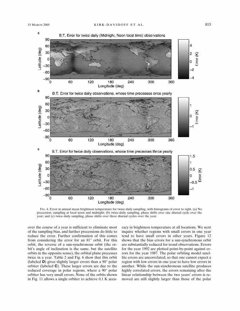
The annual mean amplitude of the semidiurnal cycleis shown in Fig. 2d. This amplitude is highly correlatedwith that of the diurnal variability, due to the asymmet-ric nature of the solar forcing of diurnal variability.Although the diurnal and semidiurnal components ofbrightness temperature variations are small relative tothe total variance, they can introduce large errors intoobservations of annual mean brightness temperature.Figure 4 shows the errors in the annual mean brightnesstemperature that result if the GCI data are sampledtwice daily. Figure 4a shows results for twice daily sam-pling at fixed times (local noon and midnight). Note thesimilarity of the pattern of error magnitude to the pat-tern of the semidiurnal cycle amplitude. In Fig. 4b, thesampling times advance through the day at a rate of 24h yr1, while in Fig. 4c, they advance at a rate of 72 hyr1. Clearly, twice-daily sampling at fixed local timeproduces a far worse estimate of the annual mean thandoes sampling at varying times of day, but the speed ofprecession is of little consequence. This demonstratesthat there is little annual variation in the phase of thediurnal brightness temperature cycle, since any suchvariations would combine with variation in the time ofday of observations to give substantially larger errorsfor a single diurnal precession per year than for severalprecessions per year.

The large, spurious diurnal and semidiurnal vari-ability in the regions at the edges of the range ofgeostationary satellites is due to details of the dataprocessing algorithm’s substitution of polar for geosta-tionary satellite data (M. Salby 2001, personal commu-nication). Because this large spurious semidiurnalvariation will increase sampling errors, especially forsun-synchronous orbits, the use of the GCI data as aproxy for real brightness temperature variability resultsin an overestimate of the mean. However, the equallylarge errors over continental regions derive from realvariability, so the conclusions we draw about which or-bits best reduce sampling error are not affected by thespurious contributions.

Figure 5 shows that some observation times are bet-

FIG. 1. Equator-crossing times as a function of Julian date forthree different orbits, as indicated.


FIG. 2. (a) 1992 annual mean of global cloud imagery 11-�m brightness temperature, (b) standard deviation of brightnesstemperature, (c) amplitude of diurnal cycle, and (d) amplitude of semidiurnal cycle.


Fig 2 live 4/C

ter than others. It shows the observation time depen-dence of the standard deviation of the errors shown fornoon and midnight observations in Fig. 4a. Clearly, asingle sun-synchronous satellite making fixed time-of-day observations will more closely approximate thetrue average brightness temperature if its equatorcrossing times are set to 4 A.M./P.M. or 10 A.M./P.M.,rather than 1 A.M./P.M. or 7 A.M./P.M. These times cor-respond to the nodes of the semidiurnal cycle in bright-ness temperature averaged over those regions wherethe diurnal cycle is of substantial amplitude (greaterthan 3 K).

4. Results and discussion

Our results are summarized in Figs. 6–9 and Tables1–3. They present the statistical properties of the sam-pling errors modeled for a range of orbital parametersand for different sampling periods. We are looking forthose orbital configurations that can recover brightnesstemperature with the fewest grid-point errors largerthan 0.1 K. We are interested both in the absolute ac-curacy, and in the accuracy of difference from one yearto the next. The grid resolution is 15° latitude by 30°longitude. Table 1 defines the alphabetical labels forthe various orbit and scanning combinations. Tables 2and 3 show the standard deviation over all grid squares,of sampling errors for mean, diurnal minimum, and di-urnal range of brightness temperature. Figures 6–9show the distribution of these grid-square errors. In thefigures, the errors are shown for three different years(1987, 1988, and 1992), or three year-to-year differ-ences (1988–87, 1992–87, 1992–88), while in the Tables2 and 3, the mean of standard deviations for the threeyears—or three differences—is shown. For both thetables and figures, various averaging periods, orbits,

numbers of satellites, and sampling patterns (nadir orcross-track scanning) are shown. In Figs. 6–9, for eachdistribution, the central dot corresponds to the medianof the grid-square errors, and the lines extend from theminimum to the 25th percentile and from the 75th per-centile to the maximum error.

a. Errors of annual means

Figures 10 and 11 show annual mean errors for asingle satellite in various orbits. Figures 10 and 11ashow the impact of spatial averaging on errors. In eachfigure, errors for a single sun-synchronous satellite with2 A.M./P.M. equator-crossing times are shown. In Fig. 10,the standard deviation of the errors is 3.8 K. Much ofthis error is due to random variations in the brightnesstemperature, thus, errors in adjacent grid squares areuncorrelated. If the satellite observations are averagedover larger spatial regions, the errors decrease substan-tially. Figure 11a shows errors of 15° latitude by 30°longitude grid squares. The standard deviation of theseerrors is reduced to 0.5 K. All further results will referto brightness temperature averaged over grid squaresof this size unless otherwise noted. We will frequentlycompare errors to a standard of 0.1 K, since this accu-racy could potentially allow discrimination of regionaltrends differing by, for example, 0.5 K decade1 within2 yr, and global trends differing by 1 K century1 within10 yr.

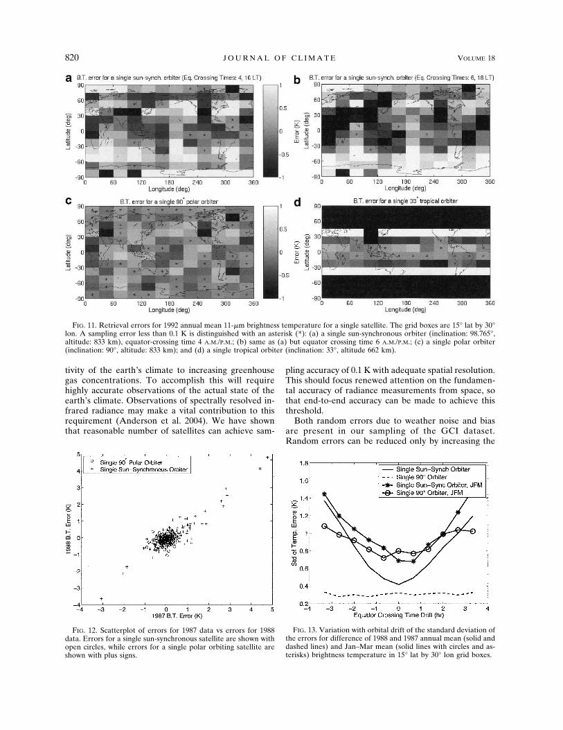
We first consider errors in annual mean brightnesstemperature for a single satellite in various orbits,shown in Fig. 11. As predicted by Fig. 5, which com-pared idealized results for different local time observa-tions, a single sun-synchronous satellite with 4 A.M./P.M.equator crossing times (Fig. 11a) does substantially bet-ter than one with 6 A.M./P.M. equator crossing times(Fig. 11b). As predicted by Fig. 4, which compares re-sults for twice-daily sampling at fixed and precessinglocal times, a single precessing polar orbiter (Fig. 11c) isclearly superior to either sun-synchronous orbiter.Comparison of these figures clearly shows the distinc-tion between random errors and errors due to aliasingof diurnal variability. If the resolution of the errors dueto twice-daily sampling shown in Figs. 4 and 5 is de-graded to 15° by 30°, we find the following. Twice orthrice yearly precessing sampling times result in errorswhose standard deviation is less than 0.1 K, while apolar orbiter, whose observation times precess twiceyearly gets errors at this resolution of over 0.2 K: thisdifference is due to the single orbiter’s inadequate totalobservation density. On the other hand, the errors forfixed local time observation explain 80% of the vari-ance in Fig. 11a, showing the role of diurnal samplingbias.

A low-latitude precessing orbiter (Fig. 11d) does notproduce substantially better annual mean brightnesstemperatures than a polar orbiter, even in the regionwhere its observations are concentrated. This is be-cause a single full precession of the time of observation

FIG. 3. Annual mean brightness temperature as a function oflocal time (interpolated from GCI data at 0000, 0300, 0600, 0900,1200, 1500, 1800, 2100 UTC) for several locations (indicated inlegend).


over the course of a year is sufficient to eliminate mostof the sampling bias, and further precessions do little toreduce the error. Further confirmation of this comesfrom considering the error for an 81° orbit. For thisorbit, the reverse of a sun-synchronous orbit (the or-bit’s angle of inclination is the same, but the satelliteorbits in the opposite sense), the orbital plane precessestwice in a year. Table 2 and Fig. 6 show that this orbit(labeled D) gives slightly larger errors than a 90° polarorbiter (labeled C). These larger errors are due to thereduced coverage in polar regions, where a 90° polarorbiter has very small errors. None of the orbits shownin Fig. 11 allows a single orbiter to achieve 0.1 K accu-

racy in brightness temperature at all locations. We nextinquire whether regions with small errors in one yeartend to have small errors in other years. Figure 12shows that the bias errors for a sun-synchronous orbitare substantially reduced for trend observations. Errorsfor the year 1992 are plotted point-by-point against er-rors for the year 1987. The polar orbiting model satel-lite errors are uncorrelated, so that one cannot expect aregion with low errors in one year to have low errors inanother. While the sun-synchronous satellite produceshighly correlated errors, the errors remaining after thelinear relationship between the two years’ errors is re-moved are still slightly larger than those of the polar

FIG. 4. Error in annual mean brightness temperature for twice-daily sampling, with histograms of error to right. (a) Noprecession, sampling at local noon and midnight; (b) twice-daily sampling, phase shifts over one diurnal cycle over theyear; and (c) twice-daily sampling, phase shifts over three diurnal cycles over the year.


orbiter (0.4 versus 0.3 K), due to interannual variabilityin the diurnal cycle.

As discussed by Leroy (2001) and by Vinnikov andGrody (2003), accuracy in interannual trends for sun-synchronous satellites is dependent on the restriction oforbit drift to small values. Figure 13 shows that whileannual means derived from precessing satellites are in-sensitive to orbital drift, drift in sun-synchronous satel-lites causes errors in year-to-year differences of about0.2 K h1 of drift in equator-crossing time. For 3-monthmeans, a 90° polar orbiter has not yet fully sampled thediurnal cycle, so errors due to drift are only slightlysmaller than for a sun-synchronous satellite.

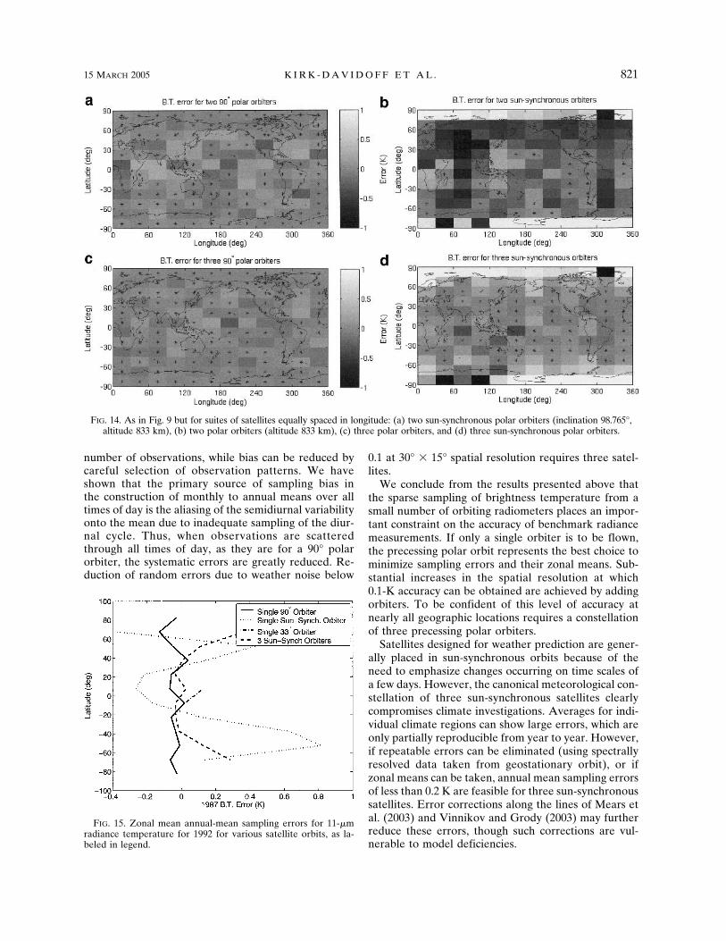
To obtain greater accuracy in retrieved brightnesstemperature, we consider the sampling errors for ob-servations by multiple satellites. Figure 14 shows resultsfor two polar satellites, orbiting at 90° angles in longi-tude, for three polar satellites orbiting at 60° angles,and for three sun-synchronous satellites orbiting at 60°angles. Two polar orbiters produce errors that are al-ways less than 0.35 K, with 65% of errors less than 0.1K. The angular separation is important for the reduc-tion of diurnal sampling bias: two sun-synchronous or-biters separated by 6 h in equator-crossing time pro-duce errors with a standard deviation of 0.2 K, whiletwo orbiters with equator crossing times of 10:30 and1:30 (the NASA Terra and Aqua orbits, respectively)produce errors of 0.7 K. Three 90° polar orbiters pro-duce errors than are always less than 0.21 K, with 84%or errors less than 0.1 K. However, for three sun-synchronous orbiters, the maximum error is 0.87 K, andonly 30% of errors are less than 0.1 K. Another way toreduce errors is to average over still larger spatial re-gions. Retrieval errors for zonal averages are given inFig. 15. Zonal mean errors are universally less than 0.1K for two or for three polar satellites, and also for a

single low-latitude orbiter. A single polar satellite, orthree sun-synchronous satellites, can attain zonal meanbrightness temperature averages with less than 0.2-Ksampling error. We have also simulated the samplingerrors of cross-track scanning satellites. For sun-synchronous orbits, these perform only marginally bet-ter than nadir-sampling satellites: for annual mean re-trieval, and a 20° wide cross-track scan, Table 2 showsthat the standard deviation of errors at 30° � 15° reso-lution is 0.20 K for three cross-track scanning satellites,and 0.21 K for three nadir-viewing satellites. As dis-cussed by Leroy (2001), cross-track scanning of practi-cal width does not extend the range of the time of day

FIG. 5. Standard deviation of grid point errors (at 0.35° lat by0.7° lon resolution) of twice-daily sampling (as in Fig. 3a) plottedas a function of time of day of the equator crossings.

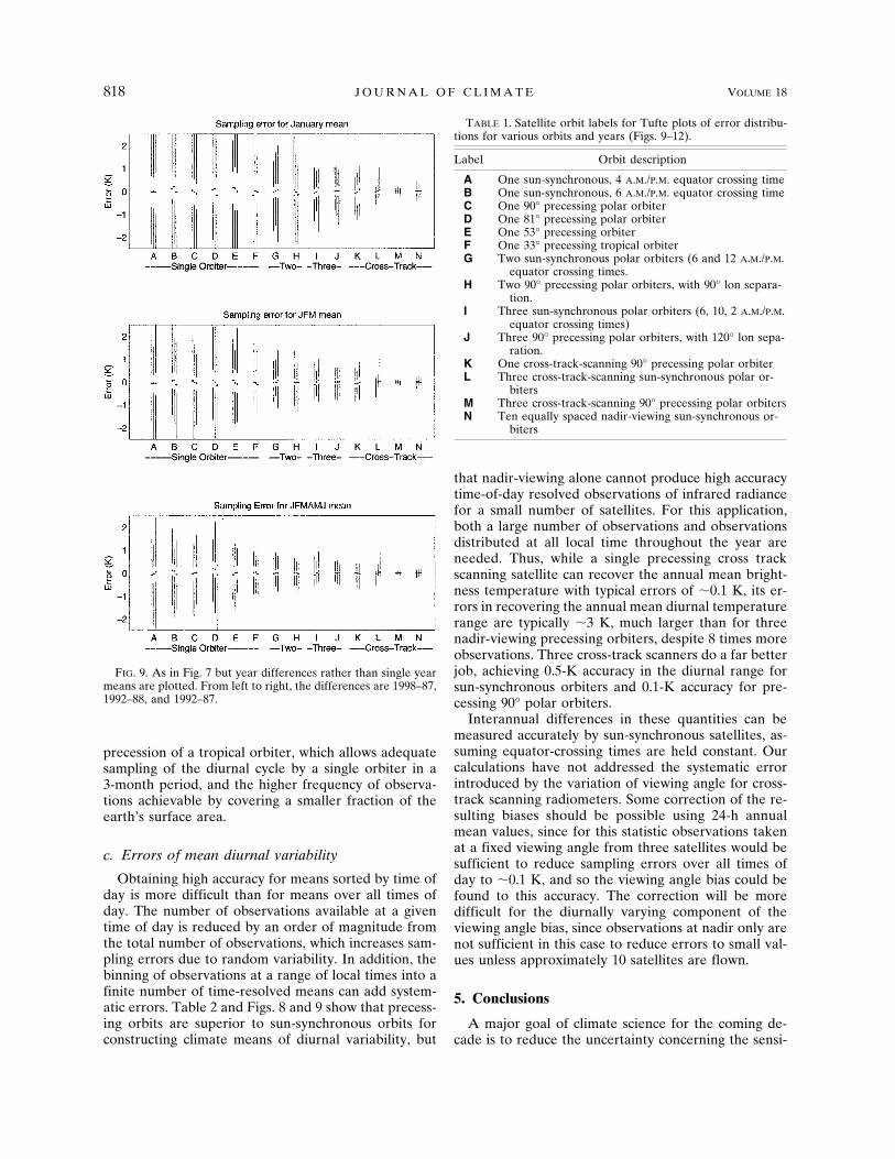
FIG. 6. The distribution of errors in mean brightness tempera-ture, average daily minimum brightness temperature, and averagediurnal brightness temperature range are plotted for a number ofsatellite orbits and for three different years. Errors are in kelvin,and are for averages over grid squares spanning 15° lat and30° lon. For each year and orbit, the lower line spans the rangefrom the minimum (largest negative) error over all grid squares tothe 25th percentile, the point shows the median error, and theupper line spans the range from the 74th percentile to the maxi-mum error. The years plotted are, from left to right, 1987, 1988,and 1992. The orbit combinations are labeled on the x axis bycapital letters, which correspond to obits shown in Table 1.


of observation sufficiently to reduce the systematic bi-ases that cause large errors for sun-synchronous orbits.For precessing orbits, systematic sampling bias hasbeen largely removed, so cross-track scanning can sub-stantially reduce errors by increasing the number ofobservations, thus reducing error due to weather noise(nonperiodic real variations in brightness temperature).Thus even a single cross-track scanning satellite in a 90°polar orbit (K) can produce brightness temperature er-rors whose standard deviation is less than 0.1 K. How-ever, the calculated errors account for sampling only,and do not take into account bias due to the angle ofview, as we discuss briefly below.

b. Errors of monthly, seasonal, and semi-annualmeans

Results for shorter averaging periods show some dis-tinct differences from those for annual means. Ofcourse, since the number of observations is smaller,

mean errors, shown in Table 3 and Figs. 8 and 9 for arange of orbital configurations and averaging periods,are correspondingly larger so that at least three satel-lites are required to achieve high accuracy. Three fur-ther results stand out. First, retrievals from polar orbit-ing satellites improve much more rapidly with increasedaveraging time than do retrievals from sun-synchronoussatellites, consistent with the strong diurnal samplingbias of sun-synchronous satellites discussed in the pre-vious section—a polar orbiter does not precess farenough in a single month to reduce diurnal samplingbias, but after 6 months a complete precession has beenaccomplished, and diurnal sampling bias is substantiallyreduced. Second, sun-synchronous satellites do sub-stantially better at retrieving differences between yearsthan at retrieving absolute brightness temperature,though still not so well as polar orbiting satellites. For a1-month average, retrievals from a single tropical or-biter produces errors much smaller than for a singlepolar orbiter, and errors comparable to those from twopolar orbiters. This follows from the relatively rapid

FIG. 7. As in Fig. 5 but year differences rather than annualmeans are plotted. From left to right, the differences are 1988–87,1992–88, and 1992–87.

FIG. 8. As in Fig. 5 but errors are for grid square mean errors forthe month of Jan, the months Jan–Mar, and the months Jan–Jun.


precession of a tropical orbiter, which allows adequatesampling of the diurnal cycle by a single orbiter in a3-month period, and the higher frequency of observa-tions achievable by covering a smaller fraction of theearth’s surface area.

c. Errors of mean diurnal variability

Obtaining high accuracy for means sorted by time ofday is more difficult than for means over all times ofday. The number of observations available at a giventime of day is reduced by an order of magnitude fromthe total number of observations, which increases sam-pling errors due to random variability. In addition, thebinning of observations at a range of local times into afinite number of time-resolved means can add system-atic errors. Table 2 and Figs. 8 and 9 show that precess-ing orbits are superior to sun-synchronous orbits forconstructing climate means of diurnal variability, but

that nadir-viewing alone cannot produce high accuracytime-of-day resolved observations of infrared radiancefor a small number of satellites. For this application,both a large number of observations and observationsdistributed at all local time throughout the year areneeded. Thus, while a single precessing cross trackscanning satellite can recover the annual mean bright-ness temperature with typical errors of �0.1 K, its er-rors in recovering the annual mean diurnal temperaturerange are typically �3 K, much larger than for threenadir-viewing precessing orbiters, despite 8 times moreobservations. Three cross-track scanners do a far betterjob, achieving 0.5-K accuracy in the diurnal range forsun-synchronous orbiters and 0.1-K accuracy for pre-cessing 90° polar orbiters.

Interannual differences in these quantities can bemeasured accurately by sun-synchronous satellites, as-suming equator-crossing times are held constant. Ourcalculations have not addressed the systematic errorintroduced by the variation of viewing angle for cross-track scanning radiometers. Some correction of the re-sulting biases should be possible using 24-h annualmean values, since for this statistic observations takenat a fixed viewing angle from three satellites would besufficient to reduce sampling errors over all times ofday to �0.1 K, and so the viewing angle bias could befound to this accuracy. The correction will be moredifficult for the diurnally varying component of theviewing angle bias, since observations at nadir only arenot sufficient in this case to reduce errors to small val-ues unless approximately 10 satellites are flown.

5. Conclusions

A major goal of climate science for the coming de-cade is to reduce the uncertainty concerning the sensi-

FIG. 9. As in Fig. 7 but year differences rather than single yearmeans are plotted. From left to right, the differences are 1998–87,1992–88, and 1992–87.

TABLE 1. Satellite orbit labels for Tufte plots of error distribu-tions for various orbits and years (Figs. 9–12).

Label Orbit description

A One sun-synchronous, 4 A.M./P.M. equator crossing timeB One sun-synchronous, 6 A.M./P.M. equator crossing timeC One 90° precessing polar orbiterD One 81° precessing polar orbiterE One 53° precessing orbiterF One 33° precessing tropical orbiterG Two sun-synchronous polar orbiters (6 and 12 A.M./P.M.

equator crossing times.H Two 90° precessing polar orbiters, with 90° lon separa-

tion.I Three sun-synchronous polar orbiters (6, 10, 2 A.M./P.M.

equator crossing times)J Three 90° precessing polar orbiters, with 120° lon sepa-

ration.K One cross-track-scanning 90° precessing polar orbiterL Three cross-track-scanning sun-synchronous polar or-

bitersM Three cross-track-scanning 90° precessing polar orbitersN Ten equally spaced nadir-viewing sun-synchronous or-

biters


TABLE 3. Standard deviation of 30° � 15° grid box errors in BT for various orbits; for averaging periods of 1, 3, and 6 months; andfor differences from year to year.

Error of

OrbitJan

mean BTDifferences

of Jan mean BTJan–Marmean BT

Differencesof Jan–Mar mean BT

Jan–Junmean BT

Differencesof Jan–Jun mean BT

A 0.95 1.16 0.71 0.73 0.67 0.59B 1.20 1.06 1.08 0.68 1.05 0.56C 1.28 0.97 0.56 0.64 0.37 0.47D 1.06 1.39 0.62 0.85 0.45 0.61E 0.95 1.28 0.55 0.69 0.39 0.49F 0.80 1.01 0.46 0.68 0.35 0.47G 0.44 0.52 0.33 0.32 0.31 0.25H 0.45 0.53 0.22 0.31 0.14 0.20I 0.36 0.39 0.27 0.25 0.23 0.20J 0.28 0.38 0.15 0.22 0.11 0.16K 0.58 0.44 0.54 0.25 0.17 0.15L 0.25 0.17 0.22 0.13 0.22 0.12M 0.04 0.05 0.02 0.03 0.02 0.02N 0.13 0.13 0.13 0.07 0.13 0.05

TABLE 2. Standard deviation of 30° � 15° grid box errors for annual mean, annual mean minimum, and annual mean diurnal rangeof brightness temperature (BT) and for year-to-year differences.

Errors of

OrbitAnnual

mean BT

Differencesof annualmean BT

Annual meanminimum BT

Differencesof annual mean

minimum BTAnnual mean

diurnal BT range

Differencesof annual mean

diurnal BT range

A 0.56 0.42 4.18 1.87 — 1.28B 1.01 0.40 2.51 0.78 — 0.48C 0.26 0.33 1.51 1.21 2.85 1.81D 0.30 0.43 1.05 1.19 1.40 1.48E 0.32 0.34 0.79 1.00 1.28 1.52F 0.25 0.35 0.72 1.00 1.11 1.53G 0.26 0.17 1.89 0.91 — 0.96H 0.11 0.15 0.45 0.55 0.52 0.65I 0.20 0.16 1.06 0.52 — 0.59J 0.07 0.10 0.31 0.38 0.29 0.37K 0.09 0.11 1.31 1.02 2.61 1.84L 0.21 0.11 0.68 0.30 0.53 0.28M 0.01 0.01 0.08 0.10 0.11 0.15N 0.04 0.03 0.12 0.15 0.14 0.17

FIG. 10. Retrieval errors for annual mean 11-�m brightness temperature for a single sun-synchronous satellite.


tivity of the earth’s climate to increasing greenhousegas concentrations. To accomplish this will requirehighly accurate observations of the actual state of theearth’s climate. Observations of spectrally resolved in-frared radiance may make a vital contribution to thisrequirement (Anderson et al. 2004). We have shownthat reasonable number of satellites can achieve sam-

pling accuracy of 0.1 K with adequate spatial resolution.This should focus renewed attention on the fundamen-tal accuracy of radiance measurements from space, sothat end-to-end accuracy can be made to achieve thisthreshold.

Both random errors due to weather noise and biasare present in our sampling of the GCI dataset.Random errors can be reduced only by increasing the

FIG. 11. Retrieval errors for 1992 annual mean 11-�m brightness temperature for a single satellite. The grid boxes are 15° lat by 30°lon. A sampling error less than 0.1 K is distinguished with an asterisk (*): (a) a single sun-synchronous orbiter (inclination: 98.765°,altitude: 833 km), equator-crossing time 4 A.M./P.M.; (b) same as (a) but equator crossing time 6 A.M./P.M.; (c) a single polar orbiter(inclination: 90°, altitude: 833 km); and (d) a single tropical orbiter (inclination: 33°, altitude 662 km).

FIG. 12. Scatterplot of errors for 1987 data vs errors for 1988data. Errors for a single sun-synchronous satellite are shown withopen circles, while errors for a single polar orbiting satellite areshown with plus signs.

FIG. 13. Variation with orbital drift of the standard deviation ofthe errors for difference of 1988 and 1987 annual mean (solid anddashed lines) and Jan–Mar mean (solid lines with circles and as-terisks) brightness temperature in 15° lat by 30° lon grid boxes.


number of observations, while bias can be reduced bycareful selection of observation patterns. We haveshown that the primary source of sampling bias inthe construction of monthly to annual means over alltimes of day is the aliasing of the semidiurnal variabilityonto the mean due to inadequate sampling of the diur-nal cycle. Thus, when observations are scatteredthrough all times of day, as they are for a 90° polarorbiter, the systematic errors are greatly reduced. Re-duction of random errors due to weather noise below

0.1 at 30° � 15° spatial resolution requires three satel-lites.

We conclude from the results presented above thatthe sparse sampling of brightness temperature from asmall number of orbiting radiometers places an impor-tant constraint on the accuracy of benchmark radiancemeasurements. If only a single orbiter is to be flown,the precessing polar orbit represents the best choice tominimize sampling errors and their zonal means. Sub-stantial increases in the spatial resolution at which0.1-K accuracy can be obtained are achieved by addingorbiters. To be confident of this level of accuracy atnearly all geographic locations requires a constellationof three precessing polar orbiters.

Satellites designed for weather prediction are gener-ally placed in sun-synchronous orbits because of theneed to emphasize changes occurring on time scales ofa few days. However, the canonical meteorological con-stellation of three sun-synchronous satellites clearlycompromises climate investigations. Averages for indi-vidual climate regions can show large errors, which areonly partially reproducible from year to year. However,if repeatable errors can be eliminated (using spectrallyresolved data taken from geostationary orbit), or ifzonal means can be taken, annual mean sampling errorsof less than 0.2 K are feasible for three sun-synchronoussatellites. Error corrections along the lines of Mears etal. (2003) and Vinnikov and Grody (2003) may furtherreduce these errors, though such corrections are vul-nerable to model deficiencies.

FIG. 15. Zonal mean annual-mean sampling errors for 11-�mradiance temperature for 1992 for various satellite orbits, as la-beled in legend.

FIG. 14. As in Fig. 9 but for suites of satellites equally spaced in longitude: (a) two sun-synchronous polar orbiters (inclination 98.765°,altitude 833 km), (b) two polar orbiters (altitude 833 km), (c) three polar orbiters, and (d) three sun-synchronous polar orbiters.


These limitations apply to radiances that originate atthe surface or at clouds and which have large diurnalvariations. Radiances that are not affected by clouds orthe surface (e.g., MSU radiances, or GPS radio occul-tation) may show smaller errors. For these, sun-synchronous satellites may provide acceptable climatedata.

Acknowledgments. The authors are grateful to MurrySalby for the use of his Global Cloud Imagery dataset.

Support has been provided by NASA Grant NAG5-8779, and NOAA Contract 50-SPNA-1-00042. Helpfulreviews by Stephen Leroy and an anonymous reviewerimproved the clarity and completeness of this paper.

REFERENCES

Anderson, J. G., J. Dykema, R. M. Goody, H. Hu, and D. B.Kirk-Davidoff, 2004: Absolute, spectrally resolved, thermalradiance: A benchmark for climate monitoring from space. J.Quant. Spectrosc. Radiat. Transfer, 85, 367–383.

Chang, T. C., L. S. Chiu, C. Kummerow, J. Meng, and T. T.Wilheit, 1998: First results of the TRMM Microwave Imager(TMI) monthly oceanic rain rate: comparison with SSM/I.Geophys. Res. Lett., 26, 2379–2382.

Christy, J. R., R. W. Spencer, W. B. Norris, W. D. Braswell, and

D. E. Parker, 2003: Error estimates of version 5.0 of MSU-AMSU bulk atmospheric temperatures. J. Atmos. OceanicTechnol., 20, 613–629.

Hanel, R. A., B. J. Conrath, V. G. Kunde, C. Prabhakara, I.Revah, V. V. Salomonson, and G. Wolford, 1972: The Nim-bus 4 infrared spectroscopy experiment, Part I: Calibratedthermal emission spectra. J. Geophys. Res., 77, 2629–2641.

Haskins, R., R. M. Goody, and L. Chen, 1999: Radiance covari-ance and climate models. J. Climate, 12, 1409–1422.

Heiskanen, W. A., and H. Moritz, 1967: Physical Geodesy. W.H.Freeman and Company, 364 pp.

Leroy, S. S., 2001: The effects of orbital precession on remoteclimate monitoring. J. Climate, 40, 4330–4337.

Mears, C. A., M. C. Schabel, and F. J. Wentz, 2003: Analysis of theMSU channel 2 tropospheric temperature record. J. Climate,16, 3650–3664.

Salby, M. L., H. H. Hendon, K. Woodberry, and K. Tanaka, 1991:Analysis of global cloud imagery from multiple satellites.Bull. Amer. Meteor. Soc., 72, 467–480.

——, and P. Callaghan, 1997: Sampling error in climate propertiesderived from satellite measurements: Consequences of undersampled diurnal variability. J. Climate, 10, 18–35.

Vinnikov, K. Y., and N. C. Grody, 2003: Global warming trend ofmean tropospheric temperature observed by satellites. Sci-ence, 302, 269–272.

——, A. Robock, N. C. Grody, and A. Basist, 2004: Analysis ofdiurnal and seasonal cycles and trends in climatic recordswith arbitrary observation times. J. Geophys. Res., 31,L06205, doi:10.1029/2003GL019196.


analysis of sampling errors for climate monitoring satellitesdankd/jclimatesampling.pdf · analysis...

Documents