appendix a: the head injury transportation straight to...

Appendices

331

APPENDIX A: THE HEAD INJURY TRANSPORTATION STRAIGHT TO NEUROSURGERY

(HITSNS) STUDY

A.1 BACKGROUND

The HITSNS study investigated the clinical and cost effectiveness of prehospital triage and

bypass, compared with selective secondary transfer, in apparently stable adults with suspected

significant TBI injured near to NSAHs.[1, 2] The study addressed two complementary research

questions. Firstly, in Stream A, a pilot pragmatic cluster randomised controlled trial examined

whether it was feasible to conduct a definitive trial investigating these interventions. Secondly,

in Stream B, reported in this thesis, an economic evaluation was conducted to identify the

optimal management strategy based on currently available evidence and emerging HITSNS

Stream A data. This appendix describes the methods of the HITSNS pilot study in detail and

briefly reports the Stream A results.

A.2 HITSNS PILOT STUDY METHODOLOGY

A.2.1 Setting

The trial was conducted in two separate English ambulance services: NEAS; and in the

Lancashire and Cumbrian regions of the NWAS. Each ambulance service operates in a mixed

geographical area including rural and urban populations. The NEAS region encompassed two

SNCs and eight NSAHs. The NWAS region was served by a single SNC and three NSAHs.

Participating study hospitals are listed in Table A1.

Table A1. Hospitals participating in the HITSNS study

Region Specialist neuroscience centres Non-specialist acute hospitals

NEAS Royal Victoria Hospital, Newcastle North Tyneside District Hospital

James Cook University Hospital, Middlesbrough Queen Elizabeth Hospital, Gateshead

South Tyneside District Hospital

Sunderland Royal Hospital

Wansbeck General Hospital

University Hospital of North Durham

Darlington Memorial Hospital

University Hospital of North Tees

NWAS Royal Preston Hospital Blackburn Royal Infirmary

Blackpool Victoria Hospital

Royal Lancaster Hospital

332

A.2.2 Inclusion criteria

Patients were enrolled in the study if they were injured nearest to a NSAH, but not greater

than one hours land ambulance journey from a SNC, and attended by land ambulance

personnel with suspected significant head injury (external signs of head trauma or reduced

GCS score ≤12). Patients meeting these criteria but thought to be aged <16 years or have life

threatening injuries causing unstable airway, breathing or circulation were excluded. ABC

instability was defined as:

Partial or complete airway obstruction after simple airway manoeuvre, or requirement

for a supraglottic airway device at the scene of injury

Respiratory rate <12 or >30, or sucking chest wound, or signs of tension pneumothorax

Significant external haemorrhage not controlled by pressure, or amputation above the

wrist or ankle, or absence of a radial pulse on palpation.

Regional trauma networks were introduced in England during the planning phase of the study.

Original inclusion criteria were therefore modified prior to the commencement of recruitment

to give consistency with major trauma triage rules and avoid confusion. NWAS instituted a

lower respiratory rate for exclusion of <10 breaths per minute (instead of <12). NEAS included

patients with a higher GCS score ≤13 (instead of ≤12). Inclusion criteria are presented in detail

in Table A2.

333

Table A2. HITSNS inclusion and exclusion criteria

Inclusion criteria Exclusion criteria

TBI: TBI:

Signs of significant TBI: External evidence of head

injury with GCS≤13*, open skull or depressed skull

fracture.

No signs of significant TBI: External evidence of

head injury, but GCS>13, no open or depressed

skull fracture.

Clinical: Clinical:

No overt ABC compromise† (No PH airway

obstruction, no intubation, RR 12-30bpm†, No

sucking chest wound, no tension pneumothorax, no

amputation above wrist/ankle, no absence of radial

pulse‡)

Overt ABC compromise† (Any of PH: airway

obstruction, intubation, RR <12 or >30bpm,

sucking chest wound, tension pneumothorax,

amputation above wrist/ankle, absence of radial

pulse)

Location: Location:

Injured nearest to NSAH and <1 hours travel time of

a SNC.

Injured nearest to SNC, or >1 hours travel time of

a SNC.

Demographic: Demographic:

Adult, appearing >16 years old Child, appearing <16 years old

EMS: EMS:

Attended by EMS in land ambulance Not attended by EMS. Attended by air

ambulance, or other non-land ambulance EMS

vehicle

*NWAS GCS inclusion criterion ≤12. †NWAS RR criteria 10-30 . RR: Respiratory rate; bpm: breaths per

minute; ABC: airway, breathing, or circulation; PH: prehospital

A.2.3 Interventions

Two management strategies were compared: pre-hospital triage and bypass (intervention

group); and initial transportation to the local NSAH (control group), which was current NHS

practice at the time the study was designed. Treatment subsequent to arrival at the initial

hospital was at the discretion of local clinicians and was not prescribed. The fundamental

differences between these pathways are the differential timing and quality of resuscitation and

definitive care. Prehospital triage and bypass expedites access to acute neurosurgery and

neurocritical care, and may also increase the number of patients’ receiving ostensibly superior

specialist treatment. However, risks of secondary brain injury from deterioration during

prolonged prehospital transportation, and over-triage of patients not requiring specialist care,

are conceivable disadvantages.

334

A training programme was delivered to ambulance service personal outlining the background,

objectives and design of the HITSNS study, detailing trial procedures, identifying required roles

and responsibilities, and highlighting the position of the HITSNS trial procedures within

regional trauma systems. Training within NEAS was primarily by self-directed learning

packages, online training modules, and divisional level teaching of team leaders. Uptake of

training was monitored by self-certified completion of training, with a minimum of 70% of staff

receiving training targeted. Mandatory paper-based teaching packages were subsequently

mailed to uncertified ambulance personnel who remained untrained once this goal was

reached. In contrast, individual face-to-face training was performed in NWAS, made possible

by the lower number of paramedics that required training.

A.2.4 Randomisation

The potentially time critical nature of significant TBI and the challenging prehospital

environment precluded the use of individual randomisation, and unit of service cluster

randomisation based on ambulance station was therefore used to allocate patients to each

intervention. Forty six ambulance stations from NEAS, and 28 from NWAS, were allocated to

different interventions using one:one matched pair randomisation based on distance from the

nearest NSAH, distance from nearest SNC, and number of full time ambulances. In the event of

paramedics rotating to different a station, treatment allocation was ultimately determined

according to the base ambulance station of the senior attending paramedic.

A.2.5 Recruitment

Patients were identified for trial inclusion using a combination of prospective and retrospective

procedures. Paramedics attending patients in the field could directly notify study personal of

patients meeting study inclusion criteria. Trained research paramedics also screened all

electronic ambulance service report forms on a daily basis to identify cases that contained free

text terms possibly related to significant TBI, or where trauma ‘pre-alerts’ had been issued to

receiving hospitals. Recruitment commenced in NEAS on the 1st January 2012, with full

participation of all clusters by 1st April 2012. Full recruitment in NWAS started immediately on

the 18th April 2012. Enrolment finished in both ambulance services on the 31st March 2013.

The acceptable recruitment rate required in the pilot study to demonstrate feasibility was

informed by the theoretical power calculation of a future definitive trial with unfavourable

outcome on the extended GOS as the primary endpoint. The following assumptions were

made: a 30% event rate in the control group, a two-tailed 5% absolute difference in

unfavourable GOS outcome, intracluster correlation of 0.02; cluster size of 35; no loss to follow 335

up; power of 80% to avoid a type II error; and a 5% risk of a type I error. Four thousand two

hundred patients (2,100 in each study arm) would consequently be required, enrolled from

120 ambulance stations in four ambulance services over three years. As the HITSNS study was

conducted in two ambulances services over a single year recruitment of 700 patients was

envisaged.

A.2.6 Outcomes

There were five primary outcomes of the HITSNS Stream A pilot study, which examined the

following feasibility endpoints.

Acceptable recruitment rate: The monthly recruitment rate should exceed 50% of that

necessary for a definitive trial. Based on sample size calculations, 350 patients

recruited over 12 months with an increasing monthly recruitment rate was considered

acceptable.

Prevalence of significant TBI patients: The proportion of patients with significant TBI in

each arm should be greater than 80%.

Compliance with treatment allocation: Non-compliance with management pathway

allocation should not exceed 10% in each study arm.

Selection bias: Prognostic factors should be balanced across each study group and

between compliant/non-compliant patients.

Acceptability: There should be no difference in the acceptability of the studied

management pathways to patients, families or staff.

Secondary outcomes were 30 day mortality, six month extended GOS score and EQ5D three

level version, using the UK tariff for utility values. These outcomes would form the basis of any

definitive HITSNS trial. Serious adverse events were also monitored during the study.

A.2.7 Data collection

Baseline data were collected on patient demographics, injury characteristics, process

measures, management pathway, and treatments by TARN data collectors for patients

meeting TARN inclusion criteria, or by research paramedics for cases not eligible for TARN.

Data were collected using the TARN electronic Data Collection and Reporting system utilising

the procedures described previously in Chapter Three. Thirty day mortality was determined in

all patients who did not refuse consent to participate in the trial and was obtained by research

paramedics or TARN data collectors by examination of hospital notes and electronic NHS

summary of care records. Patients who consented to longer term follow up, and were 336

identified as still alive from NHS summary of care records, underwent a telephone interview by

a research paramedic or the trial manager to complete extended GOS, EQ5D and patient

satisfaction questionnaires. Research paramedics, TARN data collectors and the trial manager

had access to information about management pathways from patient notes and were

consequently unblinded as intervention allocation could be deduced.

A.2.8 Trial management

A trial protocol with a pre-specified analysis plan was registered with the NIHR. An

independent Trial Steering Group, including lay representative and experts in emergency

medicine and neurosurgery, provided overall supervision of the HITSNS study. An independent

Data Monitoring Committee assessed mortality, disability and serious adverse events

endpoints; with the power to recommend the Trial Steering Group stopped or modified the

trial. Day-to-day management of the trial was conducted by a Trial Management Group

consisting of the Chief Investigator, trial manager, statistician, research paramedics and clinical

experts from emergency medicine, neurosurgery and ambulance services.

A.2.9 Ethics, consent, and funding.

The HITNS study received ethical approval from the NHS North Wales Research Ethics

Committee (reference number: 10/WNo03/30). Good Clinical Practice recommendations and

principles from the World Medical Association Declaration of Helsinki were adhered to. [3, 4]

Patients were allocated to interventions at the scene of injury without informed consent under

the provisions of the 2005 UK Mental Capacity Act.[5, 6] ‘Opt in’ consent was subsequently

sought for follow up and inclusion of data. In patients with capacity, research paramedics or

nurses approached patients directly in hospital to obtain informed consent. Discharged

patients were contacted by post, including a study information sheet, consent form and an

invitation for a telephone interview to obtain consent. If a reply slip was returned patients

were telephoned and asked to return the signed consent form after a detailed discussion

about the study. Alternatively completed consent forms could be returned directly without an

interview. Short message service text reminders were sent by mobile phone to non-

responders. Where capacity was not recovered a personal consultee (usually next of kin), or if

unavailable a professional consultee (nominated senior health care practitioners within each

ambulance service), was approached using the same processes. Ethical approval was given to

include anonymised baseline demographic and 30 day mortality data in all patients who did

not decline consent. The trial was sponsored by the University of Manchester and funded by

the UK NIHR Health Technology Appraisal Programme.

337

A.3 HITSNS STREAM A RESULTS

A.3.1 Recruitment

In total 80,856 patients were screened for meeting HITSNS inclusion criteria. Two hundred and

ninety three eligible patients were subsequently enrolled between January 2012 and April

2013, with 256 entered from NEAS clusters and 37 recruited by NWAS ambulance stations. Of

these one hundred and sixty nine patients presented to intervention clusters (57.7%, 153

NEAS, 16 NWAS). The remaining 124 patients were enrolled from control clusters (42.3%, 103

NEAS, 21 NWAS).

Forty three of the 46 randomised NEAS clusters recruited patients with a median cluster size of

five patients. Cluster recruitment exhibited a right skewed distribution with a mode of one

patient enrolled per cluster, a minimum of zero, a maximum of 12 and an inter-quartile range

of two to eight patients. A greater number of empty clusters were evident in NWAS with only

13 from 28 randomised ambulance stations enrolling patients. NWAS clusters also

demonstrated a right skewed recruitment distribution and unequal cluster sizes with a

minimum, mode and median of zero patients, an upper quartile of one, and a maximum of

eight cases enrolled per cluster.

Complete data were available for patient age, gender, inclusion criteria variables and

compliance with treatment allocation. Of the 169 patients allocated to prehospital triage and

bypass, six declined consent for data collection (3.6%, five from NEAS, one from NWAS) and

were missing data on injury descriptions, physiology, treatment, and outcome variables.

Similarly five patients from control clusters declined consent for data collection (4.0%, all five

from NEAS). Data on 30 day mortality was unavailable in a further 10 patients (four from

Intervention clusters, six from control clusters) secondary to unknown patient identity. A much

higher level of loss to follow up was present for six month GOS and EQ5D endpoints with a

further 218 patients not replying to consent, or no contactable after giving consent (129

intervention and 89 control cases). Figure A1 presents a flow chart summarising the allocation

of clusters and derivation of study participants.

338

Figure A1. Derivation of study participants in the HITSNS pilot study

339

A.3.2 Primary outcomes

The HITSNS pilot study failed to meet several of the feasibility endpoints:

Only 293 patients were enrolled over the duration of the pilot study, reaching 83.7% of

the minimum acceptable recruitment total of 350 cases.

The vast majority of patients presenting with suspected stable significant TBI

ultimately had mild TBI. The proportion of enrolled HITSNS patients with significant TBI

thus fell far short of the specified 80% target, with only 25% (n=70, 95%CI 21-31%)

having evidence of intracranial pathology on head CT.

The target for compliance with treatment allocation was also not met, with adherence

to the prescribed management strategy observed in only of 183 of the enrolled

patients (62%, 95%CI 57-67%). Compliance varied significantly between intervention

groups, and was much higher in the control group compared with the intervention

group (81%, 95%CI 72-91%, 100/124 v 49%, 95%CI 41-57%, 83/163). Compliance also

differed markedly between trial regions with notably lower adherence in NEAS versus

NWAS (59%, 95%CI 50-66%, 150/256 v 90%, 95%CI 78-95%, 33/37).

Other feasibility outcomes were successfully achieved:

There were no clinically significant differences in case-mix between control and

interventions groups.

The studied management pathways appeared acceptable to patients, families and

staff, with high satisfaction with treatment apparent in both study groups.

A.3.3 Secondary outcomes

Marginally higher 30 day mortality was observed in the intervention group compared with

control patients, but the difference was statistically not significant (complete case, as

randomised analysis, adjusted for clustering: 9.43%, 15/159 v 8.85% 10/123, p=0.89). The

extremely high loss to follow up for assessing six month GOS and EQ5D (80.5%) precluded any

meaningful analysis of these endpoints.

340

A.4 REFERENCES

1. Lecky F RW, Fuller G, McClelland G, Pennington E, Goodacre S, Han K, Curran A, Holliman D, Freeman J, Chapman N, Stevenson M, Byers S, Mason S, Potter H, Coats T, Mackway-Jones K, Peters M, Shewan J, Strong M.: The Head Injury Transportation Straight to Neurosurgery (HITSNS) Trial - A Feasibility Study Health Technology Assessment 2014, In press.

2. Head Injury Straight to Neurosurgery Trial [http://www.hits-ns.tarn.ac.uk/]3. Hutchinson DR: ICH GCP guidelines : including other key clinical trials requirements.

[Great Britain]: Roche; 2012.4. Declaration of Helsinki. Law, medicine & health care : a publication of the American

Society of Law & Medicine 1991, 19(3-4):264-265.5. Britan GoG: Mental Capacity Act 2005. In. London; 2005.6. Alonzi A, Pringle M: Mental Capacity Act 2005, vol. 335; 2007.

341

B APPENDIX B: THE EFFECTIVENESS OF ALTERNATIVE MANAGEMENT PATHWAYS FOR

PATIENTS WITH SIGNIFICANT TRAUMATIC BRAIN INJURY – A LITERATURE REVIEW AND

SYSTEMATIC REVIEW

B.1 SUPPLEMENTARY METHODOLOGICAL INFORMATION

B.1.1 Literature search for systematic reviews and original research studies examining the

comparative effectiveness of alternative management pathways for patients with

suspected TBI

Electronic information sources

1. Cochrane library: Cochrane database of systematic reviews; Health Technology

Assessment database; Database of Abstracts of Reviews of Effects

2. Centre for Reviews and Dissemination database

3. PUBMED

4. MEDLINE

5. EMBASE

6. CINAHL

7. PROSPERO database

8. Health Technology Assessment Agency, National Institute of Clinical Excellence, MAPI

websites

9. Science Citation Index (author and citation searching)

Search limits

The MEDLINE search is listed below and was adapted for use in other data sources.

Platform: Ovid MEDLINE(R) In-Process & Other Non-Indexed Citations and Ovid MEDLINE(R)

1946 to Present

Date limits: 1975 – Week 4, 2013. Current awareness searches conducted to week 33, 2013

Other limits: Human only, no editorials/comments/letters

Search strategy

1. exp Craniocerebral Trauma/

2. ((cerebral or craniocerebral or intracranial or cranio-cerebral or intra-cranial or cranial

or head or brain or neurological) adj trauma$).ti,ab.

342

3. ((cerebral or craniocerebral or intracranial or cranio-cerebral or intra-cerebral or

cranial or head or brain or neurological) adj injur$).ti,ab.

4. (Traumatic adj ((cerebral or craniocerebral or intracranial or cranio-cerebral or intra-

cranial or cranial or head or brain or neurological) and injur$)).ti,ab.

5. (neurotrauma or neuro-trauma).ti,ab

6. 1 or 2 or 3 or 4 or 5

7. Neurosurgery/organization & administration*

8. Patient Transfer/

9. Regional Medical Programs/

10. Transportation of Patients/

11. Triage/methods*

12. *Ambulances/

13. (ambulance$ and triage).mp.

14. (prehospital adj triage).mp.

15. (pre-hospital adj triage).mp.

16. (pre-hospital adj trauma adj triage).mp.

17. (prehospital adj trauma adj triage).mp.

18. ((prehospital or pre-hospital) and triage and protocol$).mp

19. regionali?ation.ti,ab.

20. (direct adj1 (admitted or admission$)).ti,ab.

21. (direct$ adj5 transport$).ti,ab.

22. (direct$ adj5 admi$).ti,ab.

23. (hospital$ adj bypass$).mp.

24. (direct$ adj3 transfer$).mp.

25. (bypass$ adj3 protocol$).mp.

26. (trauma care system$ or rapid transfer$ or integrated transfer system$).ti,ab.

27. trauma care.ti.

28. trauma network$.ti,ab.

29. trauma system$.ti,ab

30. triage.ti,ab.

31. (direct$ adj3 transfer$).mp.

32. Trauma Centers/

33. trauma cent$.tw.

34. (regional adj2 (cent$ or unit$ or hospital$ or facilit$)).tw.

35. (speciali$ adj2 (cent$ or unit$ or hospital$ or facilit$)).tw.

36. (tertiary adj2 (cent$ or unit$ or hospital$ or facilit$)).tw.

343

37. (neurosurgical adj2 (cent$ or unit$ or hospital$ or facilit$)).tw.

38. (critical care adj (cent$ or unit$ or hospital$ or facilit$)).tw.

39. or/7-39

40. letter.pt.

41. comment.pt.

42. editorial.pt.

43. or/40-42

44. 39 not 43

45. 6 and 44

B.1.2 Systematic review examining the relative effectiveness of routine transfer and no

transfer management strategies in patients with non-surgical significant TBI injured

closest to a NSAH

Information sources

1. Cochrane Database of Systematic Reviews

2. Database of Abstracts of Reviews of Effectiveness

3. Cochrane Central Register of Controlled Trials

4. Cochrane Injuries Group Specialised Register

5. metaRegister of Controlled Trials

6. ClinicalTrials.gov

7. MEDLINE

8. EMBASE

9. CINAHL

10. Science Citation Index

11. Conference Proceedings Citation Index – Science

12. BIOSIS preview

13. SIGLE

14. Index to UK Theses

15. ProQuest Dissertation & Theses Database

16. NIHR CRN Portfolio database, NRR Archive, Health Technology Assessment Agency,

National Institute of Clinical Excellence websites

17. National Clinical Guidelines Clearing House, Scottish Intercollegiate Guidelines

Network, Australian National Health and Medical Research Council: Clinical Practice

Guidelines, Canadian Medical Association – Infobase: Clinical Practice Guidelines, New

Zealand Guidelines Group websites.

344

18. Checking reference lists of retrieved article

19. Checking reference lists of existing literature reviews

20. Correspondence with experts in the field, and relevant study authors

Search limits

The MEDLINE/EMBASE search is listed below and was adapted for use in other data sources.

Platform: Diaglog Proquest

Date limits: 1975 – Week 4, 2013. Current awareness searches conducted to week 33, 2013


Search strategy

S1 MESH.EXACT("Brain Injuries") OR MESH.EXACT("Diffuse Axonal Injury") OR

MESH.EXACT("Coma, Post-Head Injury") OR MESH.EXACT("Head Injuries, Closed") OR

MESH.EXACT("Craniocerebral Trauma -- classification")

S2 ti,ab((cerebral or craniocerebral or cranio pre/0 cerebral or cranio-cerebral or intracranial

or intra pre/0 cranial or or intra-cranial or intercranial or inter-cranial or neurological or

head$1 or brain$1) near/5 (trauma$3))



head$1 or brain$1) near/5 (injur$3))



head$1 or brain$1) near/5 (lesion$1))

S5 ti,ab((traumatic) pre/0 (cerebral or craniocerebral or cranio pre/0 cerebral or neurological

or intracranial or intra pre/0 cranial or cranio-cerebral or intra-cranial or head$1 or brain$1))

and (injur$3 or trauma or lesion$1)

S6 ti,ab((cerebral or brain$1) pre/0 (oedema$ or odema$ or edema$ or swelling))

S7 ti,ab(neurotrauma or neuro-trauma)

S8 ti,ab(TBI or SHI or severe HI)

S9 ti,ab(Diffuse axonal injur*)

S10 s1 or s2 or s3 or s4 or s5 or s6 or s7 or s8 or s9

S11 MESH.EXACT("Transportation of Patients")

S12 ti,ab((secondary or interhospital or inter-hospital or inter pre/0 hospital) pre/0 (transfer$3

or transport$5 or refer$4))

S13 MESH.EXACT("Patient Transfer") or MESH.EXACT(“Ambulances”)

345

S14 MJMESH.EXACT("Hospitalization")

S15 s11 or s12 or s13 or s14

S16 MESH.EXACT("Neurosurgery")

S17 MESH.EXACT("Neurosciences")

S18 MESH.EXACT("Intensive Care") or MESH.EXACT("Critical care")

S19 (s16 or s17) and s18

S20 ti,ab((neurological or neurosurg$4 or neuroscience$1 or specialist or trauma or

neurocritical) pre/2 (centre$1 or center$1 or service$1 or unit$1 or department$1 or care))

S21 s19 or s20

S22 MESH.EXACT("Trauma Centers") or MESH.EXACT("Hospitals, Teaching")

S23 ti,ab(specialist or neurological or neurosurg$4 or neuroscience$1 or neurocritical$2 or

neuro pre/0 critical$2 or neuro-critical$2)

S24 ti,ab(intensive pre/0 care or intensive pre/0 therap$3 or critical pre/0 care)

S25 s23 pre/0 s24

S26 s22 or s25

S27 s15 or s21 or s26

S28 MESH.EXACT("Wounds and Injuries -- mortality") OR MESH.EXACT("Craniocerebral Trauma

-- mortality")

S29 MESH.EXACT("Fatal Outcome") OR MESH.EXACT("Hospital Mortality") OR

MESH.EXACT("Survival Rate")

S30 MESH.EXACT("Glasgow Outcome Scale")

S31 MESH.EXACT("Treatment Outcome")

S32 MESH.EXPLODE("Brain Damage, Chronic")

S33 ti,ab(Outcome or mortality or death* or fatal* or morbidity or disability or unfavourable

outcome or favourable outcome or persistent vegetative state)

S34 ti,ab(Glasgow outcome scale or GOS or disability rating scale or DRS)

S35 s28 or s29 or s30 or s31 or s32 or s33 or s34

S36 s10 and s27 and s35

S37 s36 and fdb(medlineprof)

S38 EMB.EXACT("traumatic brain injury" OR "brain injury") OR EMB.EXACT("diffuse axonal

injury")

S39 s38 or s2 or s3 or s4 or s5 or s6 or s7 or s8 or s9

S40 EMB.EXACT("patient transport") or MJEMB.EXACT("hospitalization") or

EMB.EXACT("ambulance")

S41 s12 or s40

S42 EMB.EXACT("neurosurgery")

346

S43 EMB.EXACT("neuroscience")

S44 EMB.EXACT("intensive care")

S45 (s43 or s44) and s45

S46 s20 or s45

S47 EMB.EXACT("emergency health service") or EMB.EXACT("teaching hospital")

S48 s25 or s47

S49 s41 or s46 or s48

S50 EMB.EXACT("injury") OR EMB.EXACT("head injury")

S51 EMB.EXACT.EXPLODE("mortality")

S52 s50 and s51

S53 EMB.EXACT("fatality") OR EMB.EXACT("mortality") OR EMB.EXACT("survival rate") or

EMB.EXPLODE("disability")

S54 EMB.EXACT("Glasgow outcome scale")

S55 EMB.EXACT("treatment outcome")

S56 s52 or s53 or s54 or s55 or s33 or s34

S57 s39 and s49 and s56

S58 s57 and fdb(embase)

S59 s37 or s58

347

B.1.3 Risk of Bias instrument for Cohort Studies

Table B1. Risk of bias criteria for critical appraisal of cohort studies retrieved in systematic review examining the effectiveness of routine and no secondary

transfer strategies in non-surgical significant TBI

Bias domain Source of bias Very low risk of bias Low risk of bias Moderate risk of bias High risk of bias Very high risk of bias Unclear risk of bias

Selection bias a.

Outcome (or risk of outcome) influences selection of participants into exposed / non-exposed groups.

[Randomisation, with valid sequence generation & allocation concealment]

Study population is representative of the source population. Selection probabilities for exposed / unexposed group not influenced by risk of outcome.

Inclusion of participants into study groups possibly dependent on outcome, with cohorts possibly unrepresentative of source population.

Inclusion of participants into study groups is dependent on risk of outcome/ outcome, with cohorts unrepresentative of the source population.

Inclusion of participants into study groups is largely dependent on risk of outcome/outcome, with cohorts very unrepresentative of the source population.

Unable to assess risk of selection bias.

Method of selection into study groups not adequately described, or nature of cohort selection means full assessment not possible.

Selection bias b.(attrition bias)

Incomplete outcome assessment

No loss to follow up Minimal numbers lost to follow up (0-5%)

Sensitivity analysis reveals results are very robust to attrition bias.

Limited numbers lost to follow up (5 -10%)

Sensitivity analysis reveals results are robust to attrition bias.

Large numbers lost to follow up (>10%)

Sensitivity analysis reveals results are susceptible to attrition bias.

Large numbers lost to follow up (>20%)

Sensitivity analysis reveals results are very susceptible to attrition bias.

Loss to follow up and reasons for attrition not reported.

Information bias

Inaccurate measurement of exposure

Objective, validated, reliable measure for exposure

Blinded investigators

Subjective, non-validated, unreliable measure of exposure.

Exposure assessors not

Measurement of exposure not reported clearly

348

Measurement standardised between study groups

blinded to study hypothesis

Measurement not-standardised between study groups

Inaccurate measurement of outcome

Objective, validated, reliable measure for exposure

Blinded investigators

Measurement standardised between study groups

Subjective, non-validated, unreliable measurement of outcomes.

Investigators not blinded to exposure status

Measurement not-standardised between study groups

No reliable system for detecting outcomes

Follow up length insufficient or differed between groups

Measurement of outcome not reported clearly

Confounding* Variables associated with exposure, and are causal risk factors (or surrogate marker) for the outcome, are unbalanced between study groups.

[Randomisation with valid sequence generation and allocation concealment.

Adequate sample size, balance of prognostic variables across treatment

Identification:All significant confounders pre-specified and measured.

Measurement:Objective, validated, reliable, equal, measurement of confounders across

Identification:Significant confounders largely pre-specified and measured.

Measurement:Objective, validated, reliable measurement of

Identification:Significant confounders not pre-specified or measured.

Measurement:Subjective, unvalidated, unequal, or unreliable

Identification:Significant confounders not pre-specified or measured.

Balance:Imbalance at baseline between study groups with respect to confounding variables

Identification, measurement, balance, or adjustment of confounders not sufficiently described to allow judgment of risk of bias

349

groups.

Control of pre-specified confounders in analysis]

All significant confounders identified, balanced, validly measured, and validly controlled for. Further unknown confounders extremely unlikely.

study groups.

Minimal missing confounder data (0-5%), equal across groups.

Valid Imputation of missing data e.g. Multiple imputation

Balance:Known confounders well balanced between groups.

Adjustment:Valid control of all significant confounder at design and/or analysis stage.

Unknown confounders unlikely.

Sensitivity analysis shows results are very robust to unmeasured or unknown confounders.

confounders.

Limited missing confounder data (5-15%).

Valid Imputation of lost outcomes e.g. Multiple imputation

Balance:Known confounders well balanced between groups.

Adjustment:Valid control of significant confounders at design and/or analysis stage.

Unknown confounders cannot be ruled out.

Sensitivity analysis shows results are sensitive to unmeasured or unknown confounders.

measurement of confounders.

Large amount of missing confounder data (>15%).

Ad hoc methods for imputing missing data e.g. LOCF, average value

Balance:Known confounders not balanced between groups

Adjustment:Not all significant confounders controlled for at design or analysis stage.

Method of controlling for confounder potentially not valid e.g. Propensity strata not balanced, invalid regression model development.

Unknown confounders very likely

Adjustment:No attempt to control for confounding in design or analysis.

350

Sensitivity analysis shows results are very sensitive to unmeasured or unknown confounders.

Reporting bias

Selective reporting of outcomes

All primary and secondary analyses reported, as pre-specified in protocol.

All a-priori and post-hoc analyses clearly listed in paper, but no protocol reported.

Primary and secondary analyses differ minimally from those pre-specified in protocol.

Some analyses reported in paper are labelled as a-priori or post-hoc.

Primary and secondary analyses differ slightly from those pre-specified in protocol.

Analyses not labelled a-priori or post-hoc.

Primary and secondary analyses differ moderately from those pre-specified in protocol.

Analyses not labelled a-priori or post-hoc.

Primary and secondary analyses differ significantly from those pre-specified in protocol.

Linked outcomes are obviously not reported

Obvious conflict of interest

Presence of protocol or pre-specified analyses not reported.

Conflict of interests not declared

Other sources of bias

Bias due to problems not covered elsewhere domains in the tool e.g. Performance bias in prospective cohort studies

No other potential sources of bias

Other sources of bias likely to strongly influence results.

Lack of information reported to assess additional risk of additional sources of bias

*Confounding variables considered: Age; GCS; pupils; hypoxia; hypotension; extracranial Injury; CT findings: e.g. Marshall diffuse injury score or equivalent;

coagulopathy; anaemia; hypergylceamia; comorbidity; performance status; any other relevant confounder

351

B.2 SUPPLEMENTARY RESULTS

B.2.1 Details of near miss studies

Table B2. Details of near miss studies identified during in systematic review examining the effectiveness of routine and no secondary transfer strategies in non-

surgical significant TBI

Study Design Dates, Country Region

Inclusion criteria Exclusion criteria Exposed group Unexposed group Outcomes Reason for ineligibility

Krob 1984[1] CCS 1977-1979

USA (Iowa)

All Ages

CNS related motor vehicle deaths

NR Patients receiving all treatment at ‘local hospitals’

Patients undergoing secondary transfer ‘local hospitals’ to ‘university hospitals’

1 year mortality Included paediatric patients

Surgical TBI patients included

Very high risk of bias (no adjustment for confounding)

Cooke 1995[2] PCS 1990

United Kingdom (Northern Ireland)

All ages

Injury and:ISS>16Cranio-cerebral AIS>2

Death prior to ED presentation

Patients receiving all treatment at NSAH

Patients undergoing secondary transfer from NSAH to SNC

1 year mortality Included paediatric patients


Moderate TBI (GCS 9-12) included


352



Danne 1998[3] PCS 1992-1993

Australia (Victoria)

All ages

Injury and:In-patient deathICU admission>1 body systems injured ISS>16Urgent operation for cranial, thoracic, abdominal injury

NR Patients receiving all treatment at a rural hospital

Patients undergoing secondary transfer from rural hospitals to metropolitan hospitals

Preventable or potentially preventable hospital death

Included paediatric patients


No subgroup analysis of head injured patients

?Very high risk of bias (blinding of outcome assessors not reported)

Eguare 2000[4] RCS† 1995

Ireland (Limerick)

All ages

Any head injury presenting to ED

NR Patients receiving all treatment at NSAH


GOS at discharge

In-hospital mortality



Moderate TBI (GCS 9-12) included

Very high risk of bias (no adjustment for confounding for analysis of impact of secondary transfer)

353



Mann 2001[5] RCS, CBA*, †

1985-1987, 1990-1994

USA (Oregan)

Age <80 years

ICD-9 code for:Head InjuryChest InjuryFemur/open tibia fractureSpleen/liver injury

Death within 30 minutes of ED presentation

Patients receiving all treatment at Level 3/4 trauma centre

Patients undergoing secondary transfer from level 3/4 trauma centre to level 1/2 trauma centre.

30 day mortality ?Included paediatric patients


Very high risk of bias (no adjustment for confounding for analysis of impact of secondary transfer)

Sethi 2002*[6] PCS 1999

Malaysia

Age >12 years

Injury and:Admission >72 hoursICU admissionDied in hospital

Dead on ED presentation

Patients undergoing secondary transfer

Patients directly admitted to a ‘district general hospital’

Patients directly admitted to a ‘central tertiary referral hospital’ and ‘tertiary care hospital’

Inpatient mortality

Discharge Barthel Index

?Overlapping data with Sethi 2007 study



Exposed group does not include secondary transfer patients

354



Ackca 2003[7] PCS 2001

USA (Kentucky)

Head Injury with GCS<9 NR Treatment in university hospital general ICU

Treatment in university hospital neuroscience ICU (not defined if secondary transfer, direct admission, or bypass)

In hospital mortality

LOS


Exposed group not admitted to NSAH

Unexposed group may include bypassed patients

Unexposed group did not primarily examine secondary transfers


355



McDermott 2004[8] RCS 1998-1999


Age NR

Road traffic accident and head injury AIS>2

Spinal cord injury Patients admitted to a hospital without neurosurgical unit. Unclear if includes secondary transfers

Admission to university hospital with neurosurgical unit (not defined if secondary transfer, direct admission, or bypass)

Management ‘deficiencies’ contributing to 6 month ‘neurological deficency’


Small numbers of mild and moderate TBI patients

Exposed group may include secondary transfers


Very high risk of bias (unvalidated outcome measure, not reported if blinded outcome assessment)

356



Reilly 2004[9] RCS 1998-2000

USA (New York City)

Age not specified

ICD-9 injury code

Burns

Inter-hospital transfers

Patients receiving all treatment at non-designated trauma centres

Patients bypassing NSAH, and patients directly admitted to level 1 trauma centres

In hospital mortality Surgical TBI patients included

? Included paediatric patients

?Non-designated trauma centres in exposed group had neurosurgical facilities

Unexposed group did not include secondary transfer patients


Hannan2004[10]

RCS 1996-1998

USA(New York state)

Age >13 years,Single injury of AIS>3ISS>9, and:

Any of:GCS<14SBP <90RR<10,>29PR<50,>120

Subgroup analysis performed for patients with head injury and above inclusion criteria

Injured in New York City

‘Flat vital signs’ on ED admission


Patients bypassing NSAH, and patients directly admitted to SNC.



Unexposed group did not include secondary transfer patients


357



Mackenzie2006[11]

RCS 2001-2002

USA

Age 18 – 84 years

Any AIS>3 injury

‘No vital signs’ on admission

Died within 30 minutes of hospital arrival

Presenting >24 hours after injury

>65 years with hip fractures

Burns

Non English or Spanish speaking

Incarcerated or homeless.

Patients receiving all treatment at non-trauma centre

Treatment at a trauma centre (not defined if secondary transfer, direct admission, or bypass)

Inpatient mortality

Mortality at 30, 90, and 365 days.


Unexposed group not clearly defined and may include bypassed patients

358



Tallon 2006[12] 1993-1994, 1999-2000

Canada (Nova Scotia)

Age >15 years

Motor vehicle accident and ICD-9 code for:Head InjuryChest InjuryFemur/open tibia fractureSpleen/liver injury

Hospital LOS<3 days

Patients not primarily admitted to tertiary trauma centre

Primary admission to tertiary trauma centre (not defined if direct admission, or bypass)


Severity of injuries not clearly defined


Unexposed group does not include secondary transfer patients

Exposed group may include secondary transfer patients

Level of neurosurgical coverage in non tertiary trauma centres not reported

Visca 2006[13] RCS 1997-2002

Italy (Piedmont)

Head Injury with GCS 3-8

Age not specified

‘Severe hypotension’

Brain death

‘Surgically evacuated mass lesion’


Treatment at SNC (not defined if secondary transfer, direct admission, or bypass)

Glasgow outcome scale recorded at 6 weeks to 6 months




359



Ashkenazi 2007[14] RCS 2003-2005

Israel (Hadera)

Age NR

Head Injury and ‘pathological CT head’

Mild head injury and:Discharged from EDNormal CTGCS 15




‘Treatment failure’ – delayed secondary transfer required



Large proportion of non-severe TBI

Helling 2007[15] RCS 2002-2003

USA (Missouri)

All ages

Trauma system activations and:Admission >24hoursSecondary transferIn hospital deathICU admission

NR Patients receiving all treatment at level 3 trauma centre

Treatment at level 2/3 trauma centre (not defined further if direct admission, or bypass)

In hospital mortality Included paediatric patients



Exposed group included secondary transfers from non-trauma centres


360



Newgard 2007[16] RCS 1998-2003

USA (Oregon)

Any age

Injury and:Presented to NSAH (level 3 or 4 hospital)Required hospital admissionInterhospital transfer

ED: Deaths Discharges

Missing ED disposition data

Patients receiving all treatment at NSAH, ‘late transfer’ to tertiary hospital.

Patients undergoing ‘early’ secondary transfer from NSAH to tertiary trauma hospital (level 1 or 2)

Inpatient mortality No subgroup analysis of head injured patients


’Early’/’late’ secondary transfers not defined.

Exposed group included ‘late’ secondary transfers


Pracht 2007[17] RCS 2001-2003

USA (Florida)

ICD code for trauma and assessed as ‘emergency’

Lower age limit not defined

ICD codes with ‘zero risk of mortality’

Patient assessed as ‘elective’ or ‘urgent’

Age >65

Secondary transfers

Patients receiving all treatment at ‘non-trauma centres’

Patients directly admitted to ‘designated trauma centres’ (level 1 or 2)

? Inpatient mortality (unclear)

?Included paediatric patients


Severity of injuries not clearly defined



361



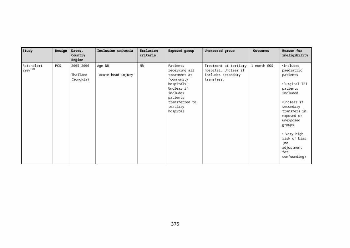
Ratanalert 2007[18] PCS 2005-2006

Thailand (Songkla)

Age NR

‘Acute head injury’

NR Patients receiving all treatment at ‘community hospitals’. Unclear if includes patients transferred to tertiary hospital

Treatment at tertiary hospital. Unclear if includes secondary transfers.

1 month GOS Included paediatric patients


Unclear if secondary transfers in exposed or unexposed groups


Sethi 2007[19] PCS Date NR

Malaysia

Age >12 years

Injury and:Admission >72 hoursICU admissionDied in hospital

Dead on ED presentation

Patients undergoing secondary transfer

Patients receiving all treatment at ‘district general hospitals’

Patients directly admitted to ‘tertiary hospitals’

Inpatient mortality

Discharge Barthel Index

Discharge Musculoskeletal Functional Assessment Index




362



Zulu 2007[20] PCS 1997-2001

South Africa (Kwa-Zulu Natal)

Age not specified

Head injury and: LOC Neurological deficit GCS<15

NR Patients receiving all treatment at NSAH



Neurological disability at discharge



Large proportion of non-severe TBI



Fabbri 2007[21] RCS 1996-2006

Italy (Forli)

Age >10 years

‘Acute head injury within 24 hours of presentation’

Requirement for immediate surgery

SBP<90mmHg

Penetrating head injury

Severe head Injury (GCS<9)



6 month GOS Included paediatric patients


Severe TBI patients excluded

363



Haas 2009[22] RCS 2001-2002

USA

Age 18 -84 years

Any injury AIS>2

Traumatic brain injury with pupil abnormality or midline shift on CT

‘No vital signs’ on admission

Died within 30 minutes of hospital arrival

Presenting >24 hours after injury

>65 years with hip fractures

Burns

Non English or Spanish speaking

Incarcerated or homeless.

Isolated gunshot wound to head

Patients receiving treatment at non-designated trauma centres

Unclear if includes patients bypassing non-trauma centres, or patients undergoing secondary transfers from non-trauma centres, or trauma centres.

Patients receiving treatment at designated trauma centres including patients undergoing secondary transfer from non-trauma centres to trauma centres, and those directly admitted to trauma centres.

Unclear if includes patients bypassing non-trauma centres, or patients undergoing secondary transfers from non-trauma centres, or trauma centres.


A significant proportion of non-designated trauma centres had neurosurgical coverage and neurosurgical ICUs

Unclear if exposed/unexposed groups include bypassed patients

Garwe 2010[23] RCS 2006-2007

USA (Oklahoma)

Age unclear

One of:ICD -9 Injury codeAIS>2ISS>8Dead on arrival to hospitalInpatient deathAdmission >48 hoursAdmitted to ICUTransferred to higher level of careTrauma team alertSurgery

Transferred from an out-of-state or non-licensed hospital

ED deaths within 1 hour of arrival

Died at scene

Isolated orthopaedic injury secondary to same level fall

Patients receiving all treatment at level 3/4 trauma centres

Patients undergoing secondary transfer from level 3/4 to level 1/2 trauma centres

30 day mortality Surgical TBI patients included


364



Meisler 2010[24] PCS 2006

Denmark (Eastern)

Age unclear

Injury and hospital trauma team activation

NR Patients receiving all treatment at local hospitals

Patients bypassing local hospitals, undergoing secondary transfer from local hospitals to level 1 trauma centre, and directly admitted to level 1 trauma centre.

30 day mortality ?Included paediatric patients



Non-exposed group included bypassed patients


Curtis 2011[25] RCS 2002-2007

Australia (New South Wales)

Age >15 years

ISS>15

Age<=15

Isolated spinal cord injury

Burns

Patients receiving all treatment at a level 3 trauma centre

Patients directly admitted to level 1 or 2 trauma centres, and a tiny number of patients undergoing secondary transfer from a level 3 trauma centre

Inpatient mortality

Hospital LOS

ICU LOS



365



Gabbe 2011a[26] RCS 2005-2006

Australia (Victoria), United Kingdom

General:Age >15 yearsHead AIS>3

Australian patients: Injury andDeathISS>15ICU >24 hoursUrgent surgery

UK patients:Injury and Admission >72 hours Admission to specialist centre Admission to ICU Death <30 days

Extracranial AIS>1

Transferred to non-participating hospital


Patients bypassing NSAH, undergoing secondary transfer from NSAH to SNC, and directly admitted to SNC.

In hospital mortality Included paediatric patients


Large proportion of moderate TBI (GCS 9-12)


366



Gabbe 2011b[27] RCS 2001-2006


United Kingdom

General:Age >15 yearsHead AIS>2ISS>15

Australian patients, injury and:DeathISS>15ICU >24 hoursUrgent surgery

UK patients, injury and: Admission >72 hours Admission to specialist centre Admission to ICU Death <30 days

Transferred to non-participating hospital


Patients bypassing NSAH, undergoing secondary transfer from NSAH to SNC, and directly admitted to SNC.




Large proportion of moderate TBI (GCS 9-12)


367

B.2.2 Detailed rationale for risk of bias assessment for included studies.

The risk of bias in included studies was determined separately according to each outcome and

assessed relative to the gold standard of an internally valid randomised controlled trial. There

is no established, validated instrument for assessing risk of bias in non-randomised studies and

a bespoke classification scheme was therefore developed for cohort studies in conjunction

with expert epidemiologists. STROBE recommendations,[28] established critical appraisal tools,[29] theoretical considerations, and empirical evidence informed the tool’s development. [30-32] To

maximise validity the tool subsequently underwent extensive independent peer review.

A methodological component approach was taken, based on the Cochrane Collaboration’s

assessment tool for risk of bias in randomised trials,[33] comprising the domains of: selection

bias, information bias, confounding, reporting bias, and other sources of bias. Risk of bias in

each domain was classified as very low, low, moderate, high, or very high risk.

Potential confounding variables were identified from a comprehensive literature review,

including systematic reviews of prognostic TBI scores.[34-38] Causal diagrams were subsequently

developed to produce a conceptual model and determine confounders requiring control in

analyses. The identified confounders were: GCS, pupil status, extracranial injury, age, hypoxia,

hypotension, coagulopathy, anaemia, hyperglycaemia, thrombocytopenia, and CT head

findings. Other potentially relevant confounders, with a less established evidence base,

include: socioeconomic status, ethnicity, medical comorbidities, neuro-worsening,

performance status, pyrexia, and hypothermia.

To assess the likelihood that outcomes had been measured but selectively not reported

protocol deviations, structurally linked outcomes, knowledge of the clinical area, and

discrepancies between methods and results sections of study reports were considered. A

review outcome matrix was subsequently completed with missing outcomes categorised

according to the ORBIT classification.[39]

Selection bias: Participant enrolment

Two studies (Patel 2005, Fuller 2011) included patients directly admitted to SNCs in the

intervention group of their reported analyses examining isolated non-surgical severe head

injuries.[40, 41] These patients will automatically receive potentially beneficial specialist care and

are therefore not relevant to the review question. Furthermore this patient group will not

undergo the hazards of inter-hospital transfer, resulting in a lower risk of adverse outcome and 368

potential overestimation of the benefit of routine secondary transfer. Harrison 2013 excluded

direct admissions to SNCs, and will therefore be at relatively lower risk of selection bias. [42]

Unpublished analyses excluding these patients were also available from Fuller 2011. [43]

Fuller 2011 and Patel 2005 included AIS>2 and intubation/ventilation on ED arrival in their

definition of severe head injury. These cohorts may therefore include patients with less severe

head trauma who underwent intubation for associated injuries, potentially biasing the

reported odds ratio away from the true effect estimate for severe TBI patients. However, Patel

2005 also reported an isolated TBI subgroup for which severe head injury is the only

conceivable rationale for intubation. Additionally in the case of Fuller 2011, using intubation in

the definition allowed inclusion of significantly head-injured patients with missing GCS, and

results were not significantly changed in a reported sensitivity analysis when intubated

patients with an admission GCS greater than nine were excluded.

It was unclear whether patients with head injuries requiring urgent neurosurgical treatment

were included in Newgard 2004,[44] with additional information unavailable by the study

authors. Patients with acute operative lesions will always be transferred for neurosurgery and

are not relevant to the review question. They may also have better prognosis than non-focal

TBI pathologies potentially biasing effect estimates.[45]

Incomplete enrolment of cases could also result in selection bias if selection probabilities into

intervention/control groups are influenced by risk of outcome. In Harrison 2013, Fuller 2011

and Patel 2005 information was submitted by data collectors for both performance

benchmarking of treatment and inclusion in study data sets. Selective recruitment of cases

could consequently be motivated by the desire to manipulate performance metrics, or result

from variations in administrative processes for different patient sub-groups. The direction and

magnitude of any ensuing selection bias is dependent on the unknown factors determining

selection, and is therefore difficult to quantify.

One study (Fuller 2011) reported marked discrepancies between trauma registry cases and

independent Hospital Episode Statistics cases suggesting incomplete enrolment. Patel 2005

used similar trauma registry data from an earlier time period, during which the discrepancy in

enrolment was even greater (T Lawrence, Trauma Audit and Research Network, personal

communication). The final study (Harrison 2013) reported an assessment for selective

enrolment in the study protocol indicating that differential recruitment into study groups was

unlikely.

369

Additional information was available on participant enrolment in Newgard 2004 from a

referenced study describing the rural trauma registry on which analyses were performed. [46]

Consecutive patients with severe head injury were identified by a detailed recruitment system

consisting of screening of emergency department logs, transferred patients, discharge

databases and hospital trauma registries. There is consequently a low risk of bias in this

domain.

Selection bias: Attrition bias

Appreciable loss to follow up was evident across all studies, with incomplete outcome data

ranging from 3% (mortality, Harrison 2013) to 16% (unfavourable outcome, Harrison 2013),

through 13% (mortality, Fuller 2011), and 9% (mortality, Patel 2005). Systematic errors could

be introduced by list wise deletion of cases with missing outcome data, if this data is not

missing completely at random (MCAR), or is not missing at random (MAR) conditional on the

included regression covariates.

In two studies (Patel 2005, Fuller 2011) the excluded patients had comparable demographic

characteristics to included patients, but patient characteristics were not presented separately

by exposure group. Fuller 2011 formally explored attrition bias and demonstrated that results

were sensitive to conservatively imputed outcomes, suggesting a plausible risk of attrition bias.

Harrison 2013 did not report any features of excluded patients but used multiple imputation,

under a ‘missing at random assumption’ to account for missing outcomes. Full details of the

imputation model were not specified and the potential for systematic differences in attrition

between study groups, and inaccurately imputed outcomes, is consequently uncertain.

Additionally available case analyses, excluding patients with missing data for explanatory

variables, could also introduce selection bias if missingness is dependent on mortality. Harrison

2013 and Fuller 2011 used multiple imputation models including outcome. An ad hoc method

of lesser validity utilising median ‘hot deck’ imputation was used by Patel 2005. No information

on loss to follow up or missing covariate data was available on from Newgard 2004 and the risk

of bias in this study is unclear for this domain.

Information bias: Exposure measurement

In all included studies information on exposure was determined from administrative records

collated by trained data collectors. In two retrospective cohort studies (Patel 2005, Fuller

370

2011) data collectors were independent of the study and unaware of the study hypothesis. In

the final study (Harrison 2013) data collectors were not blinded to the study hypothesis, but as

routinely collected, objective, and validated data were used, this is unlikely to introduce

information bias. It is unclear whether data collectors in Newgard 2004 were aware of the

study hypothesis.

Information bias: Outcome measurement

Mortality was a primary outcome in three included studies. In Patel 2005 and Fuller 2011 this

was assessed at hospital discharge or 30 days, whichever occurred first. This information is

objective and was collected by independent trained data collectors. The remaining study

(Harrison 2013) assessed mortality at six months using a combination of routine administrative

data, contacting GPs, ICU follow up services, and family questionnaires. Again, this objective

outcome measure is at low risk of information bias, despite un-blinded outcome assessors.

One study (Harrison 2013) also examined unfavourable outcome at six months as a primary

outcome. This was assessed using the extended GOS, predominantly measured by postal

questionnaires completed by patients or carers. This method of assessment has been shown to

be reliable and non-differential measurement errors, tending to bias effect estimates towards

null, are unlikely.[47] Standardised telephone interviews and consultation with ICU follow up

clinics were used to contact non-responders. The use of un-blinded outcome assessors to

partially measure such a subjective outcome may have introduced information bias. An

unusual composite endpoint comprising mortality, medical complications, and disability at

discharge was used by Newgard 2004. No information was available on the assessment of this

outcome and risk of bias is therefore unclear.

Confounding

Harrison 2013, Fuller 2011 and Patel 2005 reported significant baseline differences in

confounding variables between exposed and unexposed groups. For example marked

imbalances were observed for bilaterally dilated pupils in Harrison 2013 (22% exposed group v

10% unexposed group), abnormal respiratory rate in Fuller 2011 (23% exposed group v 16%

unexposed group), and hypotension in Patel 2005 (19% exposed group v 8% unexposed

group). The discernibly worse case mix in unexposed groups suggests a probable lack of

overlap of confounder distributions and that control of confounding is unlikely to be fully

achieved. No details were available on confounder balance from Newgard 2004.

371

Imperfect classification of explanatory variables could vitiate the control for known

confounders. Patel 2005 and Fuller 2011 only partially considered CT head scan findings,

accounted for through ISS which incorporate information on anatomical brain injuries; and

approximated hypoxia using respiratory rate. CT head findings were categorised according to

the Marshall scale in Harrison 2013, although this has prognostic value, individual CT

characteristics may provide superior control for confounding. Newgard 2004 used the AVPU

scale to measure level of consciousness rather than the more detailed Glasgow Coma Scale.

In all studies information on confounding variables was obtained from routine clinical data,

often subjectively measured by doctors. Inaccurate assessment with resulting non-differential

misclassification errors could have compromised subsequent statistical adjustments for

confounding. For example, in Harrison 2013 only moderate agreement was observed between

radiologists classifying CT head scans as normal or abnormal, with a reported kappa statistic of

0.59.

Two studies (Patel 2005, Fuller 2011) reported relatively high levels of missing confounder

data, approaching 50% for certain variables. A valid technique of multiple imputation was used

to account for missing data in the principle adjusted analysis of one of these studies (Fuller

2011), but an ad hoc method of lesser validity utilising median ‘hot deck’ imputation was used

by Patel 2005. The final study (Harrison 2013) had much lower levels of missing data which,

contingent on a valid missing at random assumption, were addressed robustly in the principle

adjusted analyses using multiple imputation No information was available on missing

confounder data in Newgard 2013.

Adjustment for confounding at the analysis stage was attempted using multivariable statistical

modelling in all studies. Harrison 2013 used standard logistic regression, while three papers

(Newgard 2004, Patel 2005, Fuller 2011) used propensity scores. Fuller 2011 and Patel 2004

additionally restricted analyses to patients with isolated head injuries and aged <65 years. The

development of multivariate models was fully described and followed consensus

recommendations in two studies (Newgard 2004, Fuller 2011). Less information was reported

in the other studies to (Patel 2005, Harrison 2012) but analyses are unlikely to be invalid.

Sensitivity analyses assessing the impact of unmeasured or unknown confounders were

reported for crude odds ratios in one study only (Fuller 2011). However, given the reported

effect sizes it is likely that unmeasured or missing confounders would require relatively high

372

prevalence and associations with exposure to lead to a non-significant result in each included

study.

Finally, as the pathophysiology of TBI has not been fully elucidated it is not possible to

construct definitive causal diagrams to fully account for confounding. Several variables with

limited evidence for potential confounding were not specified as requiring control, but are

probably associated with both transfer decisions and outcome. There are also highly likely to

be further unknown confounders. Residual confounding is therefore highly probable.

Overall a high risk of confounding bias exists across the included studies. Not all important

confounders were considered, missing data and measurement errors may have weakened the

ability to control for confounding, and clear imbalances in case-mix suggest full adjustment is

unlikely to have been achieved.

Study level reporting bias

One study (Harrison 2013) published a protocol, delineating measured outcomes but not pre-

specifying sub-group analyses. This lack of detail prevents full assessment of the presence of

reporting bias.

Patel 2005 and Fuller 2011 did not report a protocol or pre-specify an a priori analysis plan.

Mortality was the only outcome reported, and the study authors confirmed that no other end-

points were considered for the published articles. However, as the results of a single sub-group

analysis examining isolated non-surgical head injury patients were presented, but the

complementary analyses of non-isolated injuries were not reported, the potential for selective

outcome reporting cannot be excluded.

Other bias

No other sources of bias were identified in the included studies.

Overall risk of bias

In accordance with GRADE recommendations, none of the observational studies were eligible

for up- or down-grading on the basis of methodology, with all studies finally rating overall at

high risk of bias. However, for mortality analyses, the Harrison 2013 study will be at slightly

lower risk of bias, relative to the other included studies, due to prospective enrolment of

participants, exclusion of patients directly admitted to SNCs, and better control of

confounding. Conversely, Patel 2005 is relatively at slightly higher risk of bias due to greater

373

susceptibility to selection bias, very high levels of missing confounder information and a less

robust method of imputation of missing data.

B.3 REFERENCES

1. Krob MJ, Cram AE, Vargish T, Kassell NF, Davis JW, Airola S: RURAL TRAUMA CARE - A STUDY OF TRAUMA CARE IN A RURAL EMERGENCY MEDICAL-SERVICES REGION. Annals of Emergency Medicine 1984, 13(10):891-895.

2. Cooke RS, McNicholl BP, Byrnes DP: EARLY MANAGEMENT OF SEVERE HEAD-INJURY IN NORTHERN-IRELAND. Injury-International Journal of the Care of the Injured 1995, 26(6):395-397.

3. Danne P, Brazenor G, Cade R, Crossley P, Fitzgerald M, Gregory P, Kowal D, Lovell L, Morley P, Smith M et al: The major trauma management study: An analysis of the efficacy of current trauma care. Australian and New Zealand Journal of Surgery 1998, 68(1):50-57.

4. Eguare E, Tierney S, Barry MC, Grace PA: Management of head injury in a regional hospital. Irish Journal of Medical Science 2000, 169(2):103-106.

5. Mann NC, Mullins RJ, Hedges JR, Rowland D, Arthur M, Zechnich AD: Mortality among seriously injured patients treated in remote rural trauma centers before and after implementation of a statewide trauma system. Medical Care 2001, 39(7):643-653.

6. Sethi D, Aljunid S, Saperi SB, Zwi AB, Hamid H, Mustafa ANB, Abdullah AHA: Comparison of the effectiveness of major trauma services provided by tertiary and secondary hospitals in Malaysia. Journal of Trauma-Injury Infection and Critical Care 2002, 53(3):508-516.

7. Akca OH, K. ; Lenhardt, R. ; Doufas, A. G. ; Wilson, D. ; Liem, E. ; Vitaz, T. ; Heine, M. F.: Does the Care Provided by a Specialized Neuroscience ICU Improve Outcomes of Severe Traumatic Brain Injury and Ruptured Cerebral Aneurysm Patients? . ANESTHESIOLOGY 2003, 99:B16.

8. McDermott FT, Rosenfeld JV, Laidlaw JD, Cordner SM, Tremayne AB, Consultative Comm Rd Traffic F: Evaluation of management of road trauma survivors with brain injury and neurologic disability in Victoria. Journal of Trauma-Injury Infection and Critical Care 2004, 56(1):137-149.

9. Reilly JJ, Chin B, Berkowitz J, Weedon J, Avitable M: Use of a state-wide administrative database in assessing a regional trauma system: The New York City experience. Journal of the American College of Surgeons 2004, 198(4):509-518.

10. Hannan EL, Farrell LS, Cooper A, Henry M, Simon B, Simon R: Physiologic trauma triage criteria in adult trauma patients: Are they effective in saving lives by transporting patients to trauma centers? Journal of the American College of Surgeons 2005, 200(4):584-592.

11. MacKenzie EJ, Rivara FP, Jurkovich GJ, Nathens AB, Frey KP, Egleston BL, Salkever DS, Scharfstein DO: A national evaluation of the effect of trauma-center care on mortality. New England Journal of Medicine 2006, 354(4):366-378.

12. Tallon JM, Fell DB, Ackroyd-Stolarz S, Petrie D: Influence of a new province-wide trauma system on motor vehicle trauma care and mortality. Journal of Trauma-Injury Infection and Critical Care 2006, 60(3):548-552.

13. Visca A, Faccani G, Massaro F, Bosio D, Ducati A, Cogoni M, Kraus J, Servadei F: Clinical and neuroimaging features of severely brain-injured patients treated in a neurosurgical unit compared with patients treated in peripheral non-neurosurgical hospitals. British Journal of Neurosurgery 2006, 20(2):82-86.

14. Ashkenazi I, Haspel J, Alfici R, Kessel B, Khashan T, Oren M: Effect of teleradiology upon pattern of transfer of head injured patients from a rural general hospital to a neurosurgical referral centre. Emergency Medicine Journal 2007, 24(8):550-552.

374

15. Helling TS: Trauma care at rural level III trauma centers in a state trauma system. Journal of Trauma-Injury Infection and Critical Care 2007, 62(2):498-503.

16. Newgard CD, McConnell KJ, Hedges JR, Mullins RJ: The benefit of higher level of care transfer of injured patients from nontertiary hospital emergency departments. Journal of Trauma-Injury Infection and Critical Care 2007, 63(5):965-971.

17. Pracht EE, Tepas JJ, III, Celso BG, Langland-Orban B, Flint L: Survival advantage associated with treatment of injury at designated trauma centers - A bivariate probit model with instrumental variables. Medical Care Research and Review 2007, 64(1):83-97.

18. Ratanalert S, Kornsilp T, Chintragoolpradub N, Kongchoochouy S: The impacts and outcomes of implementing head injury guidelines: clinical experience in Thailand. Emergency Medicine Journal 2007, 24(1):25-30.

19. Sethi D, Aljunid S, Saperi SB, Clemens F, Hardy P, Elbourne D, Zwi AB, Res Steering C: Comparison of the effectiveness of trauma services provided by secondary and tertiary hospitals in Malaysia. Annals of Emergency Medicine 2007, 49(1):52-61.

20. Zulu BMW, Mulaudzi TV, Madiba TE, Muckart DJJ: Outcome of head injuries in general surgical units with an off-site neurosurgical service. Injury-International Journal of the Care of the Injured 2007, 38(5):576-583.

21. Fabbri A, Servadei F, Marchesini G, Stein SC, Vandelli A: Observational approach to subjects with mild-to-moderate head injury and initial non-neurosurgical lesions. J Neurol Neurosurg Psychiatry 2008, 79(10):1180-1185.

22. Haas B, Jurkovich GJ, Wang J, Rivara FP, MacKenzie EJ, Nathens AB: Survival Advantage in Trauma Centers: Expeditious Intervention or Experience? Journal of the American College of Surgeons 2009, 208(1):28-36.

23. Garwe T, Cowan LD, Neas B, Cathey T, Danford BC, Greenawalt P: Survival Benefit of Transfer to Tertiary Trauma Centers for Major Trauma Patients Initially Presenting to Nontertiary Trauma Centers. Academic Emergency Medicine 2010, 17(11):1223-1232.

24. Meisler R, Thomsen AB, Abildstrom H, Guldstad N, Borge P, Rasmussen SW, Rasmussen LS: Triage and mortality in 2875 consecutive trauma patients. Acta Anaesthesiologica Scandinavica 2010, 54(2):218-223.

25. Curtis K, Chong S, Mitchell R, Newcombe M, Black D, Langcake M: Outcomes of Severely Injured Adult Trauma Patients in an Australian Health Service: Does Trauma Center Level Make a Difference? World Journal of Surgery 2011, 35(10):2332-2340.

26. Gabbe BJ, Lyons RA, Lecky FE, Bouamra O, Woodford M, Coats TJ, Cameron PA: Comparison of Mortality Following Hospitalisation for Isolated Head Injury in England and Wales, and Victoria, Australia. Plos One 2011, 6(5).

27. Gabbe BJ, Lecky FE, Bouamra O, Woodford M, Jenks T, Coats TJ, Cameron PA: The Effect of an Organized Trauma System on Mortality in Major Trauma Involving Serious Head Injury A Comparison of the United Kingdom and Victoria, Australia. Annals of Surgery 2011, 253(1):138-143.

28. von Elm E, Altman DG, Egger M, Pocock SJ, Gotzsche PC, Vandenbroucke JP: The Strengthening the Reporting of Observational Studies in Epidemiology (STROBE) statement: guidelines for reporting observational studies. Journal of clinical epidemiology 2008, 61(4):344-349.

29. Critical Appraisal Skills Programme [http://www.casp-uk.net/]30. Rothman KJ: Epidemiology : an introduction, 2nd ed. edn. Oxford: Oxford University

Press; 2012.31. Rothman KJ, Greenland S, Lash TL: Modern epidemiology, 3rd ed. edn. Philadelphia,

Pa. ; London: Lippincott Williams & Wilkins; 2008.32. Szklo M, Nieto FJ: Epidemiology : beyond the basics, 2nd ed. edn. Sudbury, Mass.:

Jones and Bartlett Publishers; 2007.

375

33. Higgins JPT, Altman DG, Gotzsche PC, Jueni P, Moher D, Oxman AD, Savovic J, Schulz KF, Weeks L, Sterne JAC et al: The Cochrane Collaboration's tool for assessing risk of bias in randomised trials. Br Med J 2011, 343.

34. Algattas H, Huang JH: Traumatic Brain Injury pathophysiology and treatments: early, intermediate, and late phases post-injury. International journal of molecular sciences 2014, 15(1):309-341.

35. Werner C, Engelhard K: Pathophysiology of traumatic brain injury. British journal of anaesthesia 2007, 99(1):4-9.

36. Maas AIR, Stocchetti N, Bullock R: Moderate and severe traumatic brain injury in adults. Lancet Neurology 2008, 7(8):728-741.

37. Moppett IK: Traumatic brain injury: assessment, resuscitation and early management. British journal of anaesthesia 2007, 99(1):18-31.

38. Perel P, Edwards P, Wentz R, Roberts I: Systematic review of prognostic models in traumatic brain injury. BMC Med Inform Decis Mak 2006, 6:38.

39. Kirkham JJ, Dwan KM, Altman DG, Gamble C, Dodd S, Smyth R, Williamson PR: The impact of outcome reporting bias in randomised controlled trials on a cohort of systematic reviews. BMJ (Clinical research ed) 2010, 340:c365.

40. Fuller G, Bouamra O, Woodford M, Jenks T, Patel H, Coats TJ, Oakley P, Mendelow AD, Pigott T, Hutchinson PJ et al: The Effect of Specialist Neurosciences Care on Outcome in Adult Severe Head Injury: A Cohort Study. Journal of Neurosurgical Anesthesiology 2011, 23(3):198-205.

41. Patel HC, Bouamra O, Woodford M, King AT, Yates DW, Lecky FE, Trauma Audit Res N: Trends in head injury outcome from 1989 to 2003 and the effect of neurosurgical care: an observational study. Lancet 2005, 366(9496):1538-1544.

42. Harrison DA, Prabhu G, Grieve R, Harvey SE, Sadique MZ, Gomes M, Griggs KA, Walmsley E, Smith M, Yeoman P et al: Risk Adjustment In Neurocritical care (RAIN)--prospective validation of risk prediction models for adult patients with acute traumatic brain injury to use to evaluate the optimum location and comparative costs of neurocritical care: a cohort study. Health technology assessment (Winchester, England) 2013, 17(23):vii-viii, 1-350.

43. G. F: Temporal trends in head injury outcomes from 2003 to 2009 in England and Wales, and the effect of specialist neuroscience care: a cohort study. Manchester: University of Manchester; 2012.

44. Newgard CD, Hedges JR, Arthur M, Mullins RJ: Advanced statistics: the propensity score--a method for estimating treatment effect in observational research. Academic emergency medicine : official journal of the Society for Academic Emergency Medicine 2004, 11(9):953-961.

45. Steyerberg EW, Mushkudiani N, Perel P, Butcher I, Lu J, McHugh GS, Murray GD, Marmarou A, Roberts I, Habbema JDF et al: Predicting Outcome after Traumatic Brain Injury: Development and International Validation of Prognostic Scores Based on Admission Characteristics. PLoS Med 2008, 5(8):e165.

46. Mullins RJ, Hedges JR, Rowland DJ, Arthur M, Mann NC, Price DD, Olson CJ, Jurkovich GJ: Survival of seriously injured patients first treated in rural hospitals. The Journal of trauma 2002, 52(6):1019-1029.

47. Teasdale GM, Pettigrew LE, Wilson JT, Murray G, Jennett B: Analyzing outcome of treatment of severe head injury: a review and update on advancing the use of the Glasgow Outcome Scale. J Neurotrauma 1998, 15(8):587-597.

376

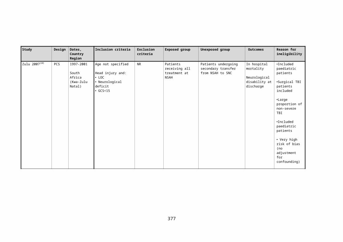
C APPENDIX C: THE PERFORMANCE OF TRIAGE RULES FOR THE PREHOSPITAL

IDENTIFICATION OF SIGNIFICANT TRAUMATIC BRAIN INJURY

C.1 COHORT STUDY INVESTIGATING THE DIAGNOSTIC ACCURACY OF PREHOSPITAL TRIAGE

RULES USING TARN DATA

C.1.1 Supplementary methodological information

Secondary analyses

A series of additional analyses were conducted to investigate the sensitivity of results to

alternative specifications of the index tests and reference standard in further complete case

analyses. The robustness of results to selection bias arising from missing data was also

explored in simulations using multiple imputation.[1]

The two variants of the HITSNS triage tool differ according to the threshold level of prehospital

GCS and respiratory rate used. Results were therefore re-calculated for the alternative NWAS

version of the triage rule in which a GCS cut point of ≤12, and a lower respiratory rate

threshold of <10 breaths per minute, is used. Prehospital hypoxia (oxygen saturations ≤93%)

was also added as an explicit criterion for ABC compromise in a repeat analysis of the NEAS

triage rule. Additionally the effect of adding mechanistic and demographic components of LAS

triage rule where TARN data were available, (entrapment, age>55 and bleeding disorder), was

also assessed.

The primary reference standard could include relatively unimportant AIS=3 brain injuries, and

exclude cases with multiple low severity brain lesions which could combine to represent

significant injury overall. A further sensitivity analysis was therefore conducted using a

modified reference standard of any brain AIS≥4, or ISS≥16 from only the recorded brain

injuries, or any neurosurgical procedure (including ICP monitoring). Furthermore, patients

without significant TBI may have sustained other non-head major trauma which could benefit

from bypass with early specialist care. In a further analysis the results were therefore

recalculated using the original triage rules and a modified reference standard including ISS≥16

or intensive care admission; in addition to brain AIS≥3 and any neurosurgical procedure. This

ISS threshold is consistent with accepted classifications of major trauma,[2] including the

definition used by English trauma systems,[3] and is compatible with similar studies in this field.

Finally, multiple imputation was performed to account for missing data, assuming a missing at

random mechanism, with primary analyses repeated.[1] Missing data mechanisms and full

technical details of the multiple imputation technique are now described in detail.

Missing Data and multiple imputation

Missing data is conventionally classified according to the framework developed by Little and

Rubin.[1] This approach defines the mechanism for data missingness according to the

relationship between the probability that data is missing for a variable and the values of other

observed data:

In data that is ‘missing completely at random’ the probability that data is missing is

independent of the value of any observed or unobserved variable, including the level

of the variable in question. Consequently there are no systematic differences between

cases with observed and missing data, and complete cases are a random subset of all

study participants. As the probability that data is missing for a given variable will often

be influenced by other demographic, clinical or treatment characteristics this

mechanism is unlikely in clinical settings.

‘Missing at random’ is formally defined as ‘the probability that data is missing is not

dependent on unobserved data, conditional on the observed data’.[1] Systematic

differences in the true value of a given variable between cases with missing and

complete data can therefore be explained by differences in the level of other

observed variables. For example missing prehospital values for systolic blood pressure

could plausibly arise from a ‘scoop and run’ approach by paramedics, with little time

to record measurements in severely injured patients. Cases with low blood pressure

values would therefore tend to have a higher probability of missing values as ISS

increased. However, within each level of injury severity missingness in systolic blood

pressure is completely random and there will be no systematic differences in the true

measurements between such cases with or without recorded values.

‘Missing not at random’ occurs where ‘the probability of data being missing does

depend on unobserved data, conditional on the observed data’.[1] Consequently, even

after controlling for the levels of other known data fields there are systematic

differences in the true value of a given variable between cases with and without

missing values. Extending the previous example, there may be other unmeasured or

378

unknown factors which influence the probability of prehospital blood pressure values

being missing. It is possible that sphygmomanometers don’t work as well at low blood

pressures and the probability of missingness in this variable will therefore depend on

the unknowable missing value of the blood pressure itself, or factors associated with

lower blood pressure readings (e.g. antihypertensives, heart failure or other

comorbidities) which may not be recorded in the dataset.

If there are differences apparent in the characteristics of cases with and without missing data

then a missing completely at random mechanism can be ruled out. However, as the true values

of incomplete variables are unknowable it is not possible to distinguish between missing at

random and missing not at random mechanisms by examination of the observed data alone.

List-wise deletion of cases with data missing at random, or missing not at random, will result in

a complete case sample that is not representative of the true complete sample, introducing a

serious risk of selection bias with consequent type I or II errors. Additionally the exclusion of

cases will result in loss of statistical power.[1]

Multiple imputation is a statistical technique which can be used to account for missing data,

assuming incomplete data is missing at random.[4] This approach simulates multiple complete

datasets which contain plausible values for the missing data, predicted using statistical

imputation models including other observed variables. A random element is incorporated to

reflect the uncertainty of these conjectural estimates. Results are calculated separately for

each imputed dataset by standard methods and are then combined using ‘Rubin’s’ rules that

compute a final point estimates for parameters of interest with an appropriate variance. [5] This

combination of results accounts for the uncertainty in the missing data within and between

the imputed datasets. If data were missing completely at random conditional on variables

included in the imputation model (i.e. a ‘missing at random’ mechanism), the selection bias

that would have arisen from complete case analyses will be removed in the simulated datasets

and valid results will be obtained.

Multiple imputation is grounded in Bayesian theory, with imputed values randomly sampled

from the posterior predictive distribution of the missing data, conditional on the observed

data.[5] This is achieved by developing an imputation model that regresses incomplete variables

on a set of variables with complete data. Alternatively, the ad hoc method of predictive mean

matching can be used, where missing values are conditionally sampled only from observed

values of the incomplete variable.[6]

379

In large datasets there is commonly missing data in a range of variables and multiple

imputation with chained equation (also known as fully conditional specification or sequential

regression multivariate imputation) is a method for generating imputed datasets in the

presence of manifold incomplete data fields.[7] Firstly imputation models are specified for each

data field with missing data, including variables which could predict the value of the missing

data, or predict the probability that the data is missing. Secondly, missing values for each

incomplete variable are replaced by random draws, with replacement, from its observed

values. Thirdly, an initial variable with missing data is regressed on the other variables included

in its imputation model. This regression is restricted to cases with complete data in the

dependent variable but includes simulated and observed data for the explanatory variables as

necessary. Fourthly, missing values in the initial variable are replaced by random ‘monte carlo’

draws from the predictive posterior distribution computed by the imputation regression

model. Fifthly, steps three and four are repeated for the next variable with missing data, but

including the imputed values of the initial variable if included in the imputation model. Sixthly,

this process is repeated for all the variables with missing data to complete a single cycle of

chained equations. To ensure stable results are achieved multiple cycles are repeated in the

seventh step, to achieve a final single imputed dataset. [6] Lastly the whole process is repeated

as many times as required to achieve the requisite number of imputed datasets. Five imputed

data sets are customarily recommended to provide valid results, based on theoretical grounds

and simulation experiments.[1, 7, 8]

Multiple imputation was performed using chained equations using the ice procedure in Stata

version 12.1 (StataCorp, College Station, USA). An inclusive and comprehensive strategy was

adopted to develop imputation models for each incomplete variable in order to increase the

plausibility of the missing at random assumption. The reference standard, all triage variables,

and any possible auxiliary data fields from the TARN dataset that might predict missingness in

studied variables or the value of the incomplete variable were included. The following

categories of auxiliary variables were considered: demographic characteristics, EMS interval,

emergency department vital signs, incident features e.g. vehicular entrapment, inter-hospital

transfer status, and clinical interventions.

The distribution of continuous variables was checked visually using histograms. Linear

regression was used for normally distributed continuous variables and predictive mean

matching used in the event of non-normality. Interval limits were used to prevent clinically

380

implausible outlying imputations. Logistic and proportional odds regressions were used for the

imputation models of binary and ordinal variables respectively. Categorical explanatory

variables were included using a set of dummy variables. Marginal estimates were of interest in

the analyses and interactions were therefore not considered in imputation models.

The extent of missing data was initially examined descriptively on a case-wise and variable-

wise basis. The characteristics of included cases was also compared with cases excluded using

summary statistics and hypothesis testing, according to the principles described previously.

Five sets of imputed data were generated and imputations were checked for consistency and

plausibility by visually comparing distributions of complete and imputed data, and examining

summary statistics. The Stata mim command was subsequently used to calculate triage rule

sensitivity and specificity, combining results from imputed data sets according to Rubin’s rules.[1]

C.1.2 Additional results

Missing data and multiple imputation

Data for demographic and injury variables included in the core TARN data set, were complete.

However, there were marked levels of missing data for physiological and clinical variables

recorded in the core or extended TARN data set. The extent of missing data for these variables

varied from 49.9% for prehospital airway status to 22.9% for prehospital GCS score. Table C1

summarises data completeness for important variables. Case-wise missingness is summarised

in Table C2, and varied from 63.2% of cases having no missing data on any variable to 20.3% of

cases missing data on five or more clinical or physiological variables necessary for calculation

of diagnostic accuracy metrics. Missing data demonstrated a non-monotone pattern.

Patients excluded due to missing triage rule parameters had similar characteristics to included

patients, but several variables showed statistically significant differences, demonstrating that

data were not missing completely at random. Notably, patients with missing data were

younger (51.7 v 55.1 years, p<0.01), less severely injured (ISS 17 v 20, p<0.01), and had lower

mortality (17.0 v 20.3, p<0.01). Other variables did not differ to a clinically significant extent.

Patient characteristics between included and excluded patients are summarised in Table C3.

Patients excluded due to unknown mode of transport were slightly less severely injured

(median ISS 17 v 20) and had lower mortality (13% v 20%), p<0.01. There were no other

clinically or statistically significant differences observed, as shown in Table C4.

381

Table C1. Data completeness for important variables in patients directly admitted by land

ambulance to TARN hospitals.

Patient characteristic Data completeness(n, %)

Age 14,293 (100%)

Gender 14,293 (100%)

Prehospital airway status 7,153 (50.1%)

Prehospital GCS 11,021 (77.1%)

Prehospital SBP 9,862 (69.0%)

Prehospital respiratory rate 10,099 (70.6%)

Prehospital hypoxia 9,025 (63.1%)

Anatomical injuries 14,293 (100%)

Head region AIS score 14,293 (100%)

Neurosurgery 14,293 (100%)

Table C2. Case-wise data completeness for variables necessary to determine triage status.

Number of variables missing Data completeness (n) (%)

0 5,376* 37.61

1 3,778 26.43

2 1,376 9.63

3 481 3.37

4 378 2.64

5+ 2,904 20.3

*Patients could be included in initial complete case analyses without full data on all variables if

triage status could be definitely assigned.

382

Table C3. Comparison of patient characteristics between included patients and cases

excluded for missing outcome or covariate data.

Study participants Otherwise eligible patients excluded due to missing data

p-value

Number of Patients 6,559* 7,734*

Age (years, median, IQR) 55.1 (33.3-78.4) 51.7 (31.1-75.5) <0.01

Gender (male, %, 95% CI) 67.5 (66.3-68.6) 70.1 (69.1-71.1) <0.01

ISS (median, IQR) 20 (16-26) 17 (14-25) <0.01

AIS head≥3 (%,95% CI) 84.0 (83.0-85.1) 81.1 (80.2-82.0) <0.01

Extracranial injury AIS≥3 (%,95% CI) 32.6 (31.4-33.7) 30.3 (29.2-31.3) <0.01

Neurosurgical procedure (%, 95% CI) 8.5 (7.8-9.1) 7.4 (6.8-8.0) 0.02

PH SBP (mmHg, mean, SD) 139 (33.8)[n=6,303]

141 (29.6)[n=3,559]

<0.01

PH RR (b/m, median, IQR) 18 (16-20) [n=6,452]

18 (16-20)[n=3,647]

0.64

PH oxygen saturations (%, median IQR) 97 (95-99)[n=5,643]

97 (95-99)[n=3,382]

0.31

PH GCS (median, IQR) 14 (9-15) 14 (9-15) [n=4,467]

0.01

Mortality (%, 95% CI)* 20.3 (19.3-21.3) [n=5,867]

17.0 (16.1-17.9) [n=6803]

<0.01

*complete case analysis unless sample size otherwise stated.

Table C4. Comparison of patient characteristics between included patients and cases

excluded for unknown mode of transport.

Study Direct admissions with unknown mode of p-

383

participants transport value

Number of Patients 6,559* 2,502*

Age (years, median, IQR) 55.1 (33.3-78.4) 56.7 (35.1-78.8) 0.08

Gender (male, %, 95% CI) 67.5 (66.3-68.6) 68.3 (66.5-70.1) 0.45

ISS (median, IQR) 20 (16-26) 17 (16-25) <0.01

AIS head≥3 (%,95% CI) 84.0 (83.0-85.1) 88.4 (87.2-89.7) <0.01

Extracranial injury AIS≥3 (%,95% CI)

32.6 (31.4-33.7) 20.9 (19.3-22.5) <0.01

Neurosurgical procedure (%, 95% CI)

8.5 (7.8-9.1) 9.7 (8.6-10.9) 0.06

PH SBP (mmHg, mean, SD) 139 (33.8)[n=6,303]

137 (29.5)[n=150]

=0.57

PH RR (b/m, median, IQR) 18 (16-20) [n=6,452]

18 (16-20)[n=137]

0.45

PH oxygen saturations (%,95% CI)

97 (95-99)[n=5,643]

97 (95-99)[n=141]

0.69

PH GCS (median, IQR) 14 (9-15) 14 (7-15)[n=188]

0.32

Mortality (%, 95% CI)* 20.3 (19.3-21.3) [n=5,867]

13.0 (11.6-14.5)[n=2,200]

<0.01


Simulated datasets demonstrated credible distributions for imputed incomplete variables, with

plausible ranges and no obvious anomalies (data not shown). Sensitivity and specificity

estimates for the identification of significant TBI using the HITSNS and LAS triage rules were

not materially changed following multiple imputation of missing data under a missing at

random assumption. The HITSNS triage instrument demonstrated a revised sensitivity of 33.7

(32.7-34.7) and a specificity of 88.6 (87.2-90.0), n=14,293. The LAS trauma triage tool’s

sensitivity was 43.9 (42.8-45.0), with a specificity of 68.1 (66.0-70.2), n=14,293.

Alternative specifications of triage rules.

Adding hypoxia as an explicit criteria for ABC compromise reduced the sensitivity of the NEAS

HITSNS triage rule to 25.9% (95%CI 24.7-27.2%, specificity 91.6%, 95%CI 89.7-93.3%). The

384

sensitivity and specificity of the NWAS variation of the HITSNS triage rule with a GCS≤12

threshold, and lower respiratory rate level of 10, were 26.8% (95%CI 25.3-28.4) and 97.3%

(95%CI 97.0-97.6) respectively.

Adding bleeding disorders (including prescribed anti-coagulants), vehicle entrapment and

age≥55 as mandatory criteria to the LAS triage rule manifestly increased sensitivity for

detection of significant TBI to 74.1% (95%CI 73.0-75.3) at the expense of decreased specificity

(30.3%, 95%CI 27.5-33.2).

Alternative specifications of the reference standard.

To examine the influence of alternative specifications of the reference standard diagnostic

accuracy metrics were recalculated using the original triage rule criteria and a modified

reference standard for significant TBI of: brain AIS≥4, ISS≥16 from brain injuries alone, or

undergoing a neurosurgical procedure. The sensitivity of the NEAS rule using this reference

standard was marginally higher at 35.0% (95%CI 33.6-36.5%), with slightly lower specificity of

81.6% (79.9-83.1%). Results for the LAS triage rule changed similarly with a slight improvement

in sensitivity to 46.1% (95%CI 44.6-47.6%) and small decrease in specificity to 64.4% (95%CI

62.4-66.4%).

The reference standard was modified in a further sensitivity analysis to include non-TBI major

trauma cases of ISS≥16 or requiring critical care, in addition to the original diagnostic criteria

for significant TBI. Sensitivity for significant TBI using the NEAS triage rule under these

conditions was similar to the primary analysis at 31.4% (95%CI 30.2-32.6%), but specificity was

much higher at 93% (95%CI 90.6-94.9). A comparable pattern was evident with the LAS triage

instrument with an almost identical sensitivity of 44.6% (95% 43.4-45.9%) and notably

improved specificity of 79.9% (76.5-83.0%).

385

C.2 INVESTIGATION OF COMPLIANCE WITH HITSNS TRIAGE RULE DECISIONS

C.2.1 Supplementary methodological information

Flow chart of HITSNS study participants

Figure C1. Derivation of study participants for the HITSNS sub-study examining compliance

with bypass.

386

C.3 REFERENCES

1. Little RJA, Rubin DB: Statistical analysis with missing data, 2nd ed. edn. Hoboken, N.J. ; [Chichester]: Wiley; 2002.

2. Palmer C: Major trauma and the injury severity score--where should we set the bar? Annual proceedings / Association for the Advancement of Automotive Medicine Association for the Advancement of Automotive Medicine 2007, 51:13-29.

3. Brohi KC, TC. Parr T.: Regional trauma systems interim guidance for commissioners. In. London: The Royal College of Surgeons of England; 2009.

4. Schafer JL: Multiple imputation: a primer. Statistical methods in medical research 1999, 8(1):3-15.

5. Little RJA, Rubin DB: Statistical analysis with missing data. New York: Wiley; 1987.6. White IR, Royston P, Wood AM: Multiple imputation using chained equations: Issues

and guidance for practice. Statistics in medicine 2011, 30(4):377-399.7. Sterne JA, White IR, Carlin JB, Spratt M, Royston P, Kenward MG, Wood AM, Carpenter

JR: Multiple imputation for missing data in epidemiological and clinical research: potential and pitfalls. Bmj 2009, 338:b2393.

8. Graham JW, Olchowski AE, Gilreath TD: How many imputations are really needed? Some practical clarifications of multiple imputation theory. Prevention science : the official journal of the Society for Prevention Research 2007, 8(3):206-213.

387

D APPENDIX D: THE EFFECT OF TIME TO RESUSCITATION AND TIME TO NEUROCRITICAL

CARE ON MORTALITY IN SIGNIFICANT HEAD INJURY

D.1 SUPPLEMENTARY METHODOLOGICAL INFORMATION

D.1.1 Regression modelling strategy for the examination of the association between EMS

interval and mortality

Multivariable logistic regression models were developed to investigate the independent effect

of EMS interval on mortality, controlling for potential case-mix differences between patients

with different prehospital times. A fully specified model was initially built incorporating

inpatient mortality within 30 days as the dependent variable, EMS interval as the exposure

variable, and potential confounding variables as additional explanatory variables. Specification

of confounders was based on potential causal relationships between EMS interval and

mortality, rather than statistical associations, and met the following conditions: [1, 2]

The variable is a risk factor for mortality following TBI; or is a surrogate measure of a

risk factor.

The variable is correlated, positively or negatively, with the duration of EMS interval,

and hence has a different distribution in different exposure groups.

The variable is not an intermediate step in the causal pathway between EMS interval

duration and mortality; and the variable is unaffected by the EMS interval.

A set of potential confounders was deduced from a literature review of TBI pathophysiology,

epidemiology, and prognostic models.[3-6] Overall, it was considered likely that paramedics

would transport younger, healthier and severely injured patients more urgently, and that old

age, comorbidities and poor performance status could be associated with longer EMS intervals

secondary to a perceived lack of treatment benefit. The following variables were therefore

pre-specified as explanatory variables: ISS, age, performance status, comorbidities, and first

recorded prehospital systolic blood pressure (SBP), GCS, pupillary responses and hypoxia

(oxygen saturations<93%).

All the designated confounders were available within the TARN database except for

performance status. Although recorded in the TARN registry, comorbidities and pupil

responses were excluded due to very high levels of missing data (>50%). A directed acyclic

graph demonstrated that conditioning on the included variables would remove all

388

confounding, except for that arising from comorbidities and performance status, assuming

correct model specification, no measurement errors, and no residual confounding arising from

incomplete control, unmeasured variables or unknown confounders.[7] The assumed causal

structure is presented in Figure D1.

Figure D1. Directed acyclic graph delineating the casual assumptions for the relationship

between EMS interval duration and mortality.

Prehospital GCS score was examined as a categorical variable to account for its ordinal nature

and fully reflect graduations in level of consciousness. EMS interval was also examined as a

categorical variable and classified into the 7 groups (<20, 20-40, 40-60,60-80,80-100, 100-120,

>120 minutes) to account for any non-linearity with the logit of mortality, and to aid

interpretation of effect estimates. Prehospital oxygen saturations were dichotomised into

<93% and ≥93% based on the clinically important diagnosis of hypoxia. [8] Categorical variables

389

were entered into the model as dummy variables compared with a baseline reference

category. The relationship between other continuous variables and the logit of mortality was

examined graphically, using locally weighted regression smoothing and exploratory plots of the

categorised confounding variables against the logit of outcome.[9] Age and ISS demonstrated an

approximately linear relationship with EMS interval and were included in the model as linear

terms. Prehospital SBP exhibited a u-shaped relationship with outcome and was transformed

using fractional polynomials to account for non-linearity. Coding of each variable is described

in Table D1.

Table D1. Coding of modelled variables in the multivariable model examining the association

between EMS interval and mortality.

Variable Coding RationaleAge Continuous Approximately linear relationship with logit of

outcome

Prehospital systolic blood pressure

Fractional polynomial term Assumption of linear relationship with logit of outcome not valid. ‘U’-shaped association observed.

Prehospital Glasgow Coma Score

Categorical Ordinal variable

Prehospital oxygen saturations

Categorised into 2 groups: <93%, ≥93%.

Categorisation produces clinically relevant groups. Sats of 92% are a recognised threshold for hypoxia.

Injury Severity Score

Continuous Approximately linear relationship with logit of outcome

EMS interval 7 categories :<20, 20-40, 40-60,60-80,80-100, 100-120, >120 minutes (reference category 40-60).

Categorisation allowed calculation of odds ratios for meaningful time periods. Reference category had highest number of cases.

The association of EMS interval categories with mortality could vary significantly at different

values of other explanatory variables e.g. there is a greater increase in mortality with longer

EMS intervals in older compared with younger patients. Clinically plausible Interactions

between EMS interval categories and age, ISS, prehospital SBP and prehospital hypoxia were

therefore pre-specified and examined together using a Wald ‘chunk’ test, [10] with a null

hypothesis that the ratio of odds ratios was 1. This approach minimises the problems of

multiple statistical testing with its inherent risk of increased family-wise type I error rate. In the

event of a significant ‘chunk’ test, assessment of each individual interaction was planned.

390

Interactions were examined first as the presence of a significant interaction precludes

evaluation of confounding arising from the relevant variable. This initial model was

hierarchically well formulated, containing all lower order components of the interaction terms.

After removal of non-significant interactions terms confounding was then assessed, without

the use of statistical testing, by determining if the estimated exposure odds ratio meaningfully

changed with deletion of each independent variable from the model. Potential non-

confounders were eliminated from the fully specified model if deletion did not change the

exposure odds ratio and resulted in a gain of precision evident from examination of the effect

estimate’s confidence interval.[10] Robust standard errors, based on the admitting SNC, were

used to calculate 95% confidence intervals for odds ratios to account for clustering of

outcomes within hospitals.[11]

Checking of the resulting logistic regression model was subsequently performed by assessing

goodness of fit, collinearity, influential observations and model over-fitting. The goodness of

fit, assessing the extent to which the model predicts the observed outcomes in the dataset,

was assessed using the Hosmer-Lemeshow statistic.[12] Collinearity, the degree to which a

modelled explanatory variable can be predicted by another covariate, was explored by

examination of the tolerance and variance inflation factor for EMS interval groups. [110]

Influential observations, which can disproportionately affect model coefficients, were

examined in a further diagnostic procedure by plotting Pregibon's delta-beta for each study

participant.[13] Bootstrapping, using 1,000 samples with replacement was also performed to

assess model stability.[10, 12, 14]

As a secondary analysis of an existing data-set was performed, a power analysis was not

appropriate and the 95% confidence intervals around the effect estimate will indicate the

precision of results. However, consideration of sample size is important for determining the

stability of the model, which signifies the extent to which parameters will vary with small

changes in the data used to derive the model. A 10:1 ratio for modelled covariates to the least

frequent outcome event is recommended as a rule of thumb for avoiding such model over-

fitting, and preventing description of idiosyncrasies of the data arising from random error

rather than a true underlying relationship.[12, 14]

391

D.1.2 Propensity score matching

Expert recommendations were followed to implement propensity score matching with the

greatest validity and precision.[15-18] Logistic regression modelling was used to estimate the

probability of individuals having EMS interval durations of less than 60 minutes. A non-

parsimonious modelling strategy was utilised including all variables available within the TARN

dataset measured during the EMS interval and potentially related to outcome or EMS interval.

These comprised: Mechanism of injury; vehicular entrapment; presence of penetrating

trauma; mode of transport; age; gender; first recorded prehospital SBP, respiratory rate, pulse

rate, and GCS; and prehospital hypoxia. Adequacy of specification of the propensity score

model was assessed by comparing exposed and unexposed subjects for important confounders

using standardised differences. In the presence of clinically significant differences the

propensity score was modified with addition of interaction terms, transformation of non-linear

variables and revision of included covariates. This iterative process was continued until

systematic differences between the two groups were reduced to a minimal level. Rubin’s

balancing score across 5 strata of propensity score was also examined. [16]

Propensity score matching was then performed within the area of common support using one-

to-one, nearest neighbour, greedy matching with replacement, within a calliper width of 0.2

times the standard deviation of the logit of the propensity score. Treatment effect in the

propensity score matched sample was then estimated by calculating the average effect of

treatment on the treated, equalling the mean of the individual causal effects only for those

receiving treatment, with absolute risk reductions and odds ratios subsequently calculated. To

account for the paired nature of the data McNemar’s test was used to test the statistical

significance of differences in proportions of mortality.[19] Finally the variance of the treatment

effect was estimated using bootstrapping with 1,000 replications to calculate 95% confidence

intervals.

D.1.3 Secondary analyses investigating the effect of EMS interval on mortality in significant

TBI

A number of additional analyses were conducted in the first sub-study examining the effect of

EMS interval on mortality in significant TBI, to investigate: the influence of missing covariate

and outcome data; examine sub-group effects; and assess alternative causal structures for the

relationship between EMS interval and mortality.

392

Complete case analyses were initially undertaken, but to account for potential selection bias

arising from listwise deletion of cases with incomplete covariate information, multiple

imputation of missing data was subsequently performed.[20] The extent of missing data in the

cohort was described by calculating the proportion of cases without values for important

demographic, injury and outcome variables. Case-wise missingness, examining the extent of

missing data in terms of the number of variables with incomplete data for each case, was also

calculated. To indicate the potential for selection bias arising from missing data, the

characteristics of the complete case sample were compared with patients excluded due to

missing data using descriptive statistics and hypothesis testing. Identical principles to those

previously described previously were used to develop the imputation model and generate

simulated imputed datasets, under a missing at random assumption. The primary regression

model and propensity score matching were then implemented in the imputed datasets with

Rubin’s rules used to derive final effect estimates as previously described.[20]

The effect of loss to follow up was also examined in a scenario analysis providing the most

optimistic assumptions on missing outcome data consistent with a positive relationship

between short EMS intervals and increased survival. Patients with missing outcomes with EMS

intervals <60minutes were all assumed to have survived, while those over 60 minutes were

assumed to have died. Complete case and adjusted multiple imputation multivariate analyses

were then repeated.

The potential for selection bias arising from incomplete patient enrolment in the TARN trauma

registry was assessed using HES data. HES is a national database containing details of all

admissions to English NHS hospitals, and includes information on demographics, diagnosis

(ICD-10 coded), and procedures.[21] Hospitals with >65% concordance between TARN and HES

data were defined as core hospital and results were recalculated using patients from only

these hospitals.

It is conceivable that EMS duration is only important in a small proportion of patients with

injuries requiring time-critical resuscitative interventions, and that the effect in this sub-

population may not be detected secondary to statistical noise in the primary study sample.

Unstable patients requiring ED resuscitation were therefore investigated in a pre-specified

subgroup analysis using the primary regression model specification. Patients identified as

unstable on ED arrival were included, with ED Instability defined as: GCS <9; SBP <90mmHg;

abnormal respiratory rate of <6 or >29; pulse rate of <50 or >120; hypoxia (sats<93%);

requirement for cardiopulmonary resuscitation; or presence of an obstructed airway or

393

respiratory distress. A further post hoc subgroup analysis examined if there was a differential

effect of EMS interval between patients transported by land or air ambulance. Adjusted odds

ratios for the association between EMS interval categories and mortality were calculated for

these subgroup analyses as above in complete case and multiple imputation analyses.

It is possible that injury severity could be directly influenced by EMS interval duration. For

example acute intracranial haematomas may expand to a greater extent in prolonged primary

transfers. This could manifest with worse CT head scans and higher ISS, in addition to

increasing the probability of death, and consequently introduce bias. A post hoc sensitivity

analysis was therefore conducted in which ISS was excluded from the multivariable model.

D.1.4 Secondary analyses investigating the effect of time to specialist care on mortality in

significant TBI.

Sensitivity analyses were again conducted to examine the influence of missing covariate data

using multiple imputation and ‘best’ and ‘worst’ case scenarios. Subgroup analyses were also

performed which examined if the effect of transfer time on mortality varied with the presence

of a major extracranial injury (pre-specified), or requirement for emergency craniotomy (post

hoc).

In an identical approach to the first sub-study, variable-wise and case-wise missing data levels

were computed; and the characteristics of complete case and excluded patients compared.

The primary regression model was then repeated in the imputed datasets. Any impact on

results from incomplete database enrolment was also examined by repeating multiple

imputation results for core hospital patients.

The effect of missing outcome data was also examined in a further sensitivity analysis. In a

‘best case’ scenario for bypass, using the multiply imputed datasets, patients with short times

to definitive care were initially assumed to have survived, with those transferred >8 hours

assumed to have died. These assumptions were then reversed in a ‘worst case’ scenario.

A final sensitivity analysis examined alternative specification of the primary regression model.

Intracranial pathology could theoretically be worsened by delayed specialist care, e.g.

expansion of intracranial haematomas, and ISS and Marshall Score could consequently lie on

the causal pathway between the exposure and outcome. The regression model was therefore

repeated omitting these variables that could contain information from after the time transfer

decisions were made.394

A pre-specified subgroup analysis examined if the effect of transfer time on mortality varied

with the presence of a major extracranial injury. Major extracranial injury was defined as any

non-cranial AIS code ≥3. The relationship between time to arrival at a specialist centre and

mortality was also separately investigated for patients undergoing emergency craniotomy for a

focal intracranial lesion, defined as Marshall score of 6 with an extradural or subdural

haematoma (high or mixed density lesion on head CT of >25cm3). These subgroups were of

specific interest as: major-extracranial injury increases the risk of secondary brain injury, which

could be exacerbated with prolonged transfer times; and expanding intracranial haematomas

are considered to be ‘time critical’ injuries.

D.2 SUPPLEMENTARY RESULTS

D.2.1 Effect of EMS interval on mortality in significant TBI

Multivariable regression model development

No interactions were identified between EMS interval and potential confounding variables

(age, ISS, prehospital SBP, prehospital hypoxia, prehospital GCS) demonstrated by a non-

significant wald ‘chunk’ test, p=0.78. Removal of covariates from the fully specified model did

not appreciably improve precision but did alter point estimates of odds ratios for EMS interval

categories; although there were no changes in the statistical significance of any regression

coefficients. All variables were therefore retained in a fully specified final model.

There was no evidence for a lack of model fit with the Hosmer-Lemeshow statistic not reaching

statistical significance, p=1.0. Three outlying cases were identified with high Pregibon delta-

beta’s over 0.2. All of these patients were transported to hospital within 20 minutes, of whom

2 died within 30 days. Examination of patient and injury characteristics revealed no concerns

regarding the accuracy of data and no reasons for exclusion on the basis of generalisability of

results. Collinearity was not a problem with tolerance values between 0.44 and 0.95 for EMS

interval categories. The ratio of outcome events to independent variables was 20:1; well in

excess of recommended levels. Bootstrapped coefficients did not vary to a meaningful degree

suggesting that there were no concerns regarding model over-fitting.

395

Primary regression model odds ratios

Table D2. Odds ratios and 95% confidence intervals for covariates included in multivariable

model examining the association between EMS interval and mortality in patients with

significant TBI

Model variable Odds Ratio 95% CI

Number of Patients 2,804

EMS interval <20 minutes 0.60 0.08-4.47

EMS interval 20-40 minutes 0.92 0.61-1.37

EMS interval 40-60 minutes Reference: 1.0 -




EMS interval >120 minutes 0.66 0.39-1.1

Prehospital SBP FP 1st term (x−1.37) 0.23 0.06-0.91

Prehospital SBP FP 2nd term (x2−1.87 ¿ 2.06 1.29-3.28

Age 1.04 1.03-1.05

ISS 1.07 1.06-1.08

Prehospital hypoxia 2.31 1.62-3.3

GCS 3 Reference: 1.0 -

GCS 4 1.08 0.68-1.74

GCS 5 0.64 0.38-1.09

GCS6 0.56 0.36-0.9

GCS7 0.33 0.15-0.72

GCS 8 0.09 0.05-0.16

GCS 9 0.09 0.05-0.18

GCS 10 0.14 0.07-0.26

GCS 11 0.20 0.11-0.36

GCS 12 0.12 0.06-0.23

GCS 13 0.13 0.08-0.23

GCS 14 0.08 0.04-0.14

GCS 15 0.08 0.05-0.12

FP: Fractional polynomial

Secondary analyses results

There was a notable proportion of missing data for important study variables, ranging from 0%

for age and ISS to 45.1% for prehospital oxygen saturations (Table D3). Case-wise missingness

for variables included in the multivariable regression modelling varied from 39.2% of cases

396

having no missing data on any variable to 1.1% of cases missing data on all five included

covariates (Table D4).

Patients excluded from the multivariable regression analysis due to missing data had broadly

similar characteristics to included patients, but several variables showed clinically and

statistically significant differences. In particular, patients with missing data were slightly

younger (median age 44.9 v 47.5 years, p<0.01), were more likely to be male (74.2% v 70.1%,

p<0.01), had a lower proportion of hypotension (1.9% v 3.1%, p<0.01), and had lower GCS

(median GCS 10 v 13, p<0.01). There was also a statistically significant lower median duration

of EMS interval, but this appeared to be of dubious clinical importance (median EMS interval

57 v 62 minutes). Other variables did not differ to a statistically significant extent. Patient

characteristics between included and excluded patients are summarised in Table D5.

Table D3. Rates of missing data for important variables in patients directly admitted to SNCs

by EMS.

Patient characteristic Data incompleteness*(cases with missing data,

%)

Age 0 (0%)

Prehospital GCS 2,333 (33%)

Prehospital systolic blood pressure 3,026 (42%)

Prehospital hypoxia 3,227 (45%)

ISS 0 (0%)

EMS interval 2,993 (42%)

Mortality 326 (5%)

*Total eligible sample n=7,149

397

Table D4. Case-wise missingness in variables included in multivariable regression examining

he association between EMS interval and mortality

Number of variables missing Data completeness* (n) (%)

0 2,804 39.2

1 1,370 19.2

2 509 7.1

3 423 5.9

4 1,967 27.5

5 76 1.1


Table D5. Comparison of patient characteristics between included patients and cases

excluded for missing outcome or covariate data.

Complete case Otherwise eligible patients excluded due to missing data

p-value

Number of Patients 2,804 4,345*

Age (years, median, IQR) 47.2 (29-69) 44.9 (28-66) <0.01

Gender (male, %, 95% CI) 70.1 (69.2-72.6) 74.2 (72.9-75.5) <0.01

ISS (median, IQR) 25 (17-29) 25 (16-29) 0.57

Prehospital hypotension (%, 95% CI) 3.1 (2.5-3.8) 1.9 (1.5-2.3) <0.01

Prehospital hypoxia (%, 95% CI) 13.8 (12.6-15.1) 14.0 (11.9-16.0)[n=1,118]

0.92

Prehospital GCS (median, IQR) 13 (7-15) 10 (5-14)[n=2,012]

<0.01

EMS interval (mins, median, IQR) 62 (47-82) 57 (41-78)[n=4,156]

<0.01

Mortality (%, 95% CI)* 17.5 (16.1-19.0) 19.0 (17.7-20.2)[n=4,019]

0.14


Multivariable regression results were not materially different following multiple imputation,

with odds ratios for mortality not significantly differing for different EMS interval categories as

shown in Table D5 and Figure D2 (n=7,149). Of note, the point estimate for EMS interval of <20 398

minutes in the complete case analysis changed from suggesting a benefit (odds ratio 0.60) of

rapid transportation to indicating no association with mortality following multiple imputation

(odds ratio 0.97); and odds ratios for longer EMS intervals also became closer to null. Imputed

data demonstrated credible distributions for all incomplete variables, with plausible ranges

and no obvious anomalies (data not shown). An identical fully specified model to that

implemented in the primary analysis was used, with no significant interactions or differences in

functional form of covariates detected. Model diagnostics suggested no concerns.

There was virtually no change in odds ratios in a further sensitivity analysis in which patients

with missing outcomes and EMS intervals <60 minutes were assumed to have survived and

those with EMS intervals >60 minutes assumed to have died (adjusted multiple imputation

analyses, n=7,143, Figure D3 and Table D5), and vice versa.

There were 4,135 patients admitted to core TARN hospitals during the study period. Repeating

logistic regression models for these patients resulted in materially unchanged findings in both

complete case (data not shown) and multiple imputation (Table D5) analyses, with no obvious

relationship between EMS interval and mortality apparent.

The lack of association between EMS interval and mortality was also evident in adjusted

multiple imputation analyses examining patients who were unstable on ED arrival (n=3,735);

conveyed by land ambulances (n=3,735), or transported by air ambulance (n=1,331). In each of

these subgroup analyses odds ratios were similar to the original analysis for each EMS

category. Removing ISS from the primary model also did not appreciably alter results. Table D5

summarises the results from these multiple imputation secondary analyses. Qualitatively

identical results were also achieved in corresponding complete case analyses (data not shown).

Propensity score matching results were also similar following multiple imputation. The number

of matched pairs in each data set varied from 2644 to 2708. Covariate balance was satisfactory

in each imputed dataset. After combining results using Rubin’s rules the average effect on the

treated of an EMS interval <60 minutes was a non-significant 2.3% increase in mortality (95%CI

-2.2% - 6.7%).

Figure D2. Odds of death for different EMS interval categories following multiple imputation

for missing data.

399

Reference EMS interval 40-60 minutes. Odds ratios <1 favourable indicate decreased mortality.

Figure D3. Relationship between EMS interval and odds ratio for short-term mortality in

sensitivity analysis examining missing outcomes using multiply imputed data.

Reference EMS interval 40-60 minutes. Odds ratios <1 favourable indicate decreased mortality.

400

Table D5. Summary of results from primary and secondary analyses examining the association between EMS interval and mortality

EMS Interval category (minutes)

<20 20-39.9 40-59.9 60-79.9 80-99.9 100-119.9 ≥120

Analysis: Odds ratios (95%CI):

Primary regression model

Complete case(n=2,804)

0.60(0.1-3.3)

0.92(0.6-1.4)

1.0(reference)

0.75(0.6-1.1)

0.88(0.6-1.3)

0.6(0.4-1.0)

0.66(0.4-1.4)

Multiple imputation(n= 7,149)

0.97(0.5-1.9)

1.08(0.8-1.4)

1.0(reference)

0.87(0.7-1.1)

0.97(0.7-1.3)

0.79(0.6-1.1)

1.0(0.6-1.8)

Outcomes sensitivity analysis(n= 7,149)

0.98(0.5-1.9)

1.09(0.9-1.4)

1.0(reference)

0.87(0.7-1.1)

0.97(0.7-1.3)

0.80(0.6-1.1)

1.02(0.6-1.8)

Core hospitals only(Multiple imputation, n= 4,135)

0.94(0.43-2.10)

0.98(0.71-1.34)

1.0(reference)

0.78(0.59-1.02)

0.88(0.57-1.02)

0.76(0.46-1.25)

0.86(0.48-1.52)

Subgroup analyses

Land ambulance cases(Multiple imputation, n= 5,818)

1.01(0.5-2.1)

1.1(0.8-1.4)

1.0(reference)

0.82(0.7-1.0)

0.93(0.7-1.3)

0.6(0.4-0.9)

0.88(0.4-1.9)

Air ambulance cases(Multiple imputation, n= 1,331)

1.13(0.2-8.0)

1.1(0.5-2.7)

1.0(reference)

1.01(0.6-1.7)

1.00(0.5-1.9)

1.19(0.6-2.3)

1.00(0.6-1.8)

Patients unstable on ED arrival(Multiple imputation, n= 3,735)

0.77(0.4-1.5)

1.07(0.8-1.5)

1.0(reference)

0.83(0.7-1.1)

0.88(0.6-1.3)

0.70(0.4-1.1)

0.73(0.4-1.3)

Alternative model specification

ISS removed(Multiple imputation, n= 7,149)

0.59(0.1-3.0)

0.89(0.6-1.3)

1.0(reference)

0.89(0.7-1.2)

1.12(0.8-1.5)

0.77(0.5-1.2)

0.96(0.6-1.6)

401

D.2.2 Effect of time to specialist care on mortality in significant TBI.

Multivariable regression model development

No interactions were identified between time to specialist care and other explanatory

variables; and all covariates appeared to be significant confounders and were therefore

retained in a fully specified final model. There was no evidence for a lack of model fit with the

Hosmer-Lemeshow statistic not reaching statistical significance, p=0.85. Model diagnostics for

influential observations, collinearity and over-fitting were unremarkable (data not shown).

402

Primary regression model odds ratios

Table D6. Odds ratios and 95% confidence intervals for covariates included in multivariable

model examining the association between time to arrival in a SNC and mortality in patients

with significant TBI

Model variable Odds Ratio 95% CI

Number of Patients 6,116

Time to specialist care (%, 95% CI):

No transfer Reference: 1.0 -<4 hours 0.40 0.13-1.214-8 hours 0.21 0.12-0.358-16 hours 0.30 0.15-0.62>16 hours 0.57 0.15-2.22

Age 1.06 1.05-1.06ISS 1.07 1.05-1.08ED hypotension 4.44 2.61-7.55ED hypoxia 1.81 1.51-2.18GCS 3 Reference: 1.0 -

GCS 4 0.69 0.38-1.26GCS 5 0.38 0.21-0.7GCS6 0.17 0.1-0.31GCS7 0.16 0.1-0.28GCS 8 0.10 0.06-0.17GCS 9 0.09 0.05-0.16GCS 10 0.07 0.04-0.12GCS 11 0.10 0.06-0.17GCS 12 0.07 0.04-0.12GCS 13 0.03 0.02-0.05GCS 14 0.03 0.02-0.04GCS 15 0.02 0.01-0.03Traumatic subarachnoid haemorhage 1.81 1.51-2.18Intraventricular haemorrhage 1.34 1.05-1.72Marshall Score 2 Reference: 1.0 -Marshall score 3 1.47 1.11-1.96Marshall score 4 2.79 1.99-3.91Marshall score 5/6 4.63 3.72-5.76Marshall score 7* 7.24 2.36-22.24Marshall score 8* 2.48 0.36-17.22*Published TARN modification of Marshall score used/

Odds ratios <1 favourable indicate decreased mortality.

403

Secondary analysis results

There was a large proportion of missing data for variables included in the multivariable

analysis, varying from 0% for age, Marshall Score and ISS to 41.6% for the timing of secondary

transfers to SNCs (Table D7). Case-wise missingness for variables included in the multivariable

regression modelling varied from 45.4% of cases having no missing data on any variable to

4.3% of cases missing data on at least five of the included covariates (Table D8). There were

marked differences between complete case patients and those with missing data (Table D9).

Table D7. Rates of missing data for important variables in patients with significant TBI

directly initially admitted to NSAHs.

Patient characteristic Data incompleteness*(cases with missing data, %)

Age 0 (0%)

Emergency department GCS 4,538 (33.7%)

Emergency department hypotension 4,163 (30.1%)

Emergency department hypoxia 4,774 (35.5%)

ISS 0 (0%)

Marshall score 0 (0%)

Traumatic subarachnoid haemorrhage 0 (0%)

Traumatic intraventricular haemorrhage

0 (0%)

Secondary transfer timing 5,594 (41.6%)

Mortality 1,839 (13.7%)


Table D8. Case-wise missingness in variables included in multivariable regression examining

he association between secondary transfer timing and mortality

Number of variables missing Data completeness* (n) (%)

0 6,116 45.4

1 1,852 13.8

2 1,381 10.3

3 730 5.4

4 2,801 20.8

5+ 580 4.3


404

Table D9. Comparison of patient characteristics between patients included in the analysis of

significant TBI directly initially admitted to NSAHs; and cases excluded for missing outcome

or covariate data.

Complete case Otherwise eligible patients excluded due to missing data*

p-value

Number of Patients 6,116 7,344

Age (years, median, IQR) 62.9 (40.2-81.4) 47.4 (29.8-67.2) <0.01

Gender (male, %, 95% CI) 65.0 (63.8-66.2) 74.7 (73.7-75.7) <0.01

Penetrating injury (male, %, 95% CI) 1.3 (1.0-1.6) 2.0 (1.7-2.3) <0.01

ISS (median, IQR) 18 (16-25) 24 (16-26) <0.01

Extracranial injury AIS≥3 (%, 95% CI) 17.7 (16.8-18.7) 18.5 (17.6-19.4) =0.22

Traumatic subarachnoid haemorrhage (%, 95% CI)

32.3 (31.1-33.5) 31.0 (30.0-32.0) 0.09

Traumatic intraventricular haemorrhage (%, 95% CI)

9.2 (8.4-9.9) 9.8 (9.1-10.5) 0.20

Focal intracranial lesion (%, 95% CI) 17.6 (16.6-18.5) 24.9 (24.0-26.0) <0.01

ED hypotension (%, 95% CI) 2.3 (1.9-2.6) 4.6 (3.9-5.4)[n=3,181]

<0.01

ED hypoxia (%, 95% CI) 7.3 (6.6-7.9) 7.0 (6.0-8.0)[n=2,570]

0.64

ED GCS (median, IQR) 14 (11-15) 13 (8-15)[n=2,806]

<0.01

Secondary transfer time category (%, 95% CI):

No transfer 93.7 (93.1-94.3) 91.4 (90.0-92.7)

<4 hours 0.51 (0.33-0.68) 1.6 (1.0-2.2)

4-8 hours 3.6 (3.1-4.0) 4.8 (3.8-5.8)

8-16 hours 1.8 (1.5-2.1) 1.9 (1.2-2.5)

>16 hours 0.43 (0.3-0.6) 0.34 (0.0-0.6) <0.01[n=1,750]

Mortality (%, 95% CI)* 18.7 (17.7-19.7) 16.0 (15.1-17.0)[n=5,505]

<0.01


Qualitatively similar results were seen after multiple imputation of missing covariate data; with

improved survival for patients transferred to SNCs, but no obvious relationship between time

of transfer and mortality (Table D10, n=13,460). This was also the case was the sample was

405

restricted to patients treated in core TARN hospitals in both complete case (data not shown)

and multiple imputation analyses (Table D10, n=8,021).

Scenario sensitivity analyses, simulating ‘missing not at random’ mechanisms for missing

outcomes differed dramatically from the primary analysis results (Table D10, multiple

imputation sample, n=13,460). Assuming that all transferred patients with missing outcomes

who arrived in SNCs within 8 hours survived, while other patients with incomplete mortality

data had died, suggested a dose-response relationship between early transfer and survival was

possible. The opposite pattern was observed when these assumptions were reversed (Table

D10, multiple imputation sample, n=13,460).

Interestingly, omission of possible mediating variables (ISS, Marshall Score, traumatic

subarachnoid haemorrhage, and intraventricular haemorrhage) resulted in the odds ratio for

very early secondary transfer <4 hours becoming close to unity. Odds ratio point estimates for

later secondary transfer time categories were slightly less favourable but still approximated

those from the primary analysis (n=13,460, Table D10).

Subgroup analyses examining patients with isolated TBI and multiple trauma demonstrated

similar results to the primary analysis, that did not vary across strata (Table D10). A

comparable pattern was also observed in the subgroup of patients with significant TBI

requiring emergency craniotomy. For patients transferred to SNCs for neurosurgery between

4-8 hours there was a suggeston of imporved outcomes compared to earlier transfer within 4

hours of injury (4-8 hours transfer time category odds ratio 0.52, 95% CI 0.2-1.3). Outcomes

then appeared to worsen with more prolonged transfer delays for emergency craniotomy (8-

16 hours transfer time category odds ratio 1.02, 95% CI 0.3-3.2). However this analysis was

underpowered and the 95% confidence intervals for prolonged transfer times were consistent

with either a clinically significant survival benefit or increased mortality. Furthermore, these

subgroup results should be interpreted with caution secondary to the relatively high levels of

missing data. Table D10 summarises the results of secondary analyses examining the

association between secondary transfer time to SNCs and mortality.

Table D10. Summary of results from primary and secondary analyses examining the

association between secondary transfer time to SNC care and mortality.

406

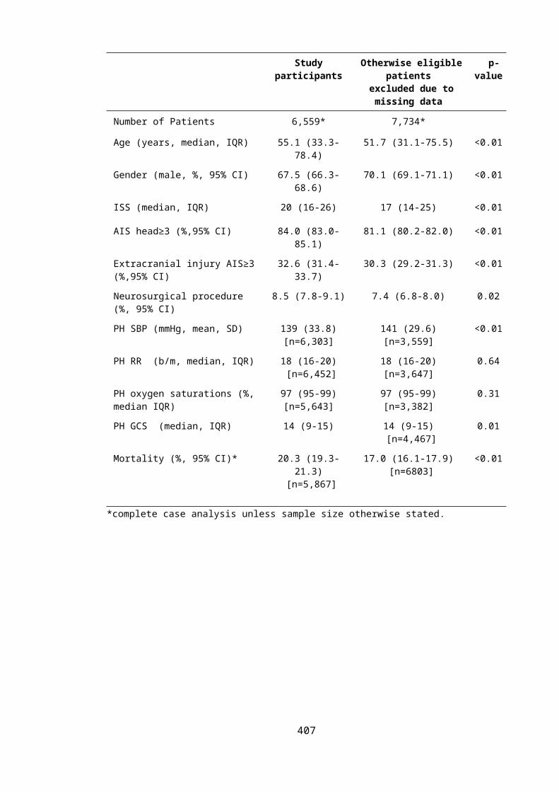
Secondary transfer timing category

No transfer

<4 hours 4- 8 hours 8-16 hours

>16 hours

Primary regression model

Complete case(n=6,006)

1.0(reference

)

0.40(0.1-1.2)

0.21(0.1-0.4)

0.30(0.2-0.6)

0.57(0.1-2.2)

Multiple imputation(n= 13,460)

1.0(reference

)

0.69(0.2-2.5)

0.31(0.2-0.6)

0.37(0.2-0.7)

0.40(0.1-1.4)

‘Best case’ outcomes sensitivity analysis(Multiple imputation, n= 13,460)

1.0(reference

)

0.19(0.1-0.4)

0.11(0.1-0.2)

1.8(1.3-2.4)

2.1(1.1-4.3)

‘Worst case’ outcomes sensitivity analysis(Multiple imputation, n= 13,460)

1.0(reference

)

6.12(3.1-12.1)

3.6(2.5-5.1)

0.28(0.1-0.6)

0.24(0.0-1.4)

Core hospitals only(Multiple imputation, n= 8,021)

1.0(reference

)

0.67(0.2-2.1)

0.29(0.1-0.6)

0.39(0.3-0.6)

0.42(0.1-1.6)

Subgroup analyses

Isolated TBI(Multiple imputation, n= 11,016)

1.0(reference

)

0.72(0.2-2.5)

0.34(0.2-0.7)

0.40(0.2-0.7)

0.40(0.1-2.0)

TBI with major extracranial injury(Multiple imputation, n= 2,444)

1.0(reference

)

0.64(0.1-3.9)

0.24(0.1-0.5)

0.29(0.1-0.8)

0.38(0.1-2.2)

TBI requiring emergency craniotomy(n= 256)

NA* 1.0(reference

)

0.52(0.2-1.3)

1.02(0.3-3.2)

-†

Alternative model specification

ISS and Marshall score removed(Multiple imputation, n= 13,460)

1.0(reference

)

1.05(0.3-4.2)

0.46(0.2-0.9)

0.57(0.3-1.1)

0.51(0.1-2.1)

Odds ratios <1 favourable indicate decreased mortality.

*All patients requiring emergency craniotomy will undergo secondary transfer to a SNC. †4 patients

were transferred after 16 hours, of whom all died, preventing inclusion in logistic regression analysis

secondary to low cell count.

D.3 REFERENCES

1. Rothman KJ, Greenland S, Lash TL: Modern epidemiology, 3rd ed. edn. Philadelphia, Pa. ; London: Lippincott Williams & Wilkins; 2008.

407

2. Szklo M, Nieto FJ: Epidemiology : beyond the basics, 2nd ed. edn. Sudbury, Mass.: Jones and Bartlett Publishers; 2007.

3. Ghajar J: Traumatic brain injury. Lancet 2000, 356(9233):923-929.4. Maas AI, Stocchetti N, Bullock R: Moderate and severe traumatic brain injury in

adults. The Lancet Neurology 2008, 7(8):728-741.5. Moppett IK: Traumatic brain injury: assessment, resuscitation and early

management. British journal of anaesthesia 2007, 99(1):18-31.6. Perel P, Edwards P, Wentz R, Roberts I: Systematic review of prognostic models in

traumatic brain injury. BMC Med Inform Decis Mak 2006, 6:38.7. Greenland S, Pearl J, Robins JM: Causal diagrams for epidemiologic research.

Epidemiology (Cambridge, Mass) 1999, 10(1):37-48.8. Warrell DA, Cox TM, Firth JD: Oxford textbook of medicine, 5th ed. / edited by David

A. Warrell, Timothy M. Cox, John D. Firth ; sub-editor Immunological mechanisms and disorders of the skin, Graham S. Ogg. edn. Oxford: Oxford University Press; 2010.

9. Cleveland W: LOWESS: A Program for Smoothing Scatterplots by Robust Locally Weighted Regression. The American Statistician 1981, 35(1).

10. Kleinbaum DG, Klein M: Logistic regression : a self-learning text, 2nd ed. edn. New York, NY: Springer-Verlag; 2002.

11. Wears RL: Advanced statistics: statistical methods for analyzing cluster and cluster-randomized data. Academic emergency medicine : official journal of the Society for Academic Emergency Medicine 2002, 9(4):330-341.

12. Hosmer DW, Lemeshow S, Sturdivant RX: Applied logistic regression, 3rd ed. edn. Hoboken: Wiley; 2013.

13. Pregibon D: Logistic Regression Diagnostics. 1981:705-724.14. Harrell FE: Regression modeling strategies : with applications to linear models,

logistic regression, and survival analysis. New York ; London: Springer; 2001.15. Austin PC: An Introduction to Propensity Score Methods for Reducing the Effects of

Confounding in Observational Studies. Multivariate behavioral research 2011, 46(3):399-424.

16. Guo S, Fraser MW: Propensity score analysis : statistical methods and applications. Los Angeles ; London: SAGE; 2010.

17. Williamson E, Morley R, Lucas A, Carpenter J: Propensity scores: from naive enthusiasm to intuitive understanding. Statistical methods in medical research 2012, 21(3):273-293.

18. Austin PC: Propensity-score matching in the cardiovascular surgery literature from 2004 to 2006: a systematic review and suggestions for improvement. The Journal of thoracic and cardiovascular surgery 2007, 134(5):1128-1135.

19. Austin PC: Comparing paired vs non-paired statistical methods of analyses when making inferences about absolute risk reductions in propensity-score matched samples. Statistics in medicine 2011, 30(11):1292-1301.

20. Schafer JL: Multiple imputation: a primer. Statistical methods in medical research 1999, 8(1):3-15.

21. Hospital Episode Statistics [http://www.hesonline.nhs.uk ]

408

E APPENDIX E: THE RELATIONSHIP BETWEEN PREHOSPITAL AND EMERGENCY

DEPARTMENT PHYSIOLOGY IN PATIENTS WITH SIGNIFICANT TRAUMATIC BRAIN INJURY

E.1 SUPPLEMENTARY METHODOLOGICAL INFORMATION

E.1.1 Statistical assessment of agreement

Comparison of prehospital and emergency department physiology is a challenging statistical

problem. Firstly, on the one hand, the prehospital and emergency department readings for

each vital sign are clearly related, and could be assumed to be measuring the same underlying

physiological quantity. Secondly, on the other hand, the temporal differences in assessment,

dynamic changes in clinical condition and potential influence of treatments might suggest that

measurements from each setting should alternatively be considered as distinct variables.

The first viewpoint is consistent with assessing reproducibility; the examination of variation in

repeated measurements made on a subject under changing conditions.[1] Investigation of

agreement, i.e. how close two measurements on the same subject are, within this paradigm

will address the question of whether prehospital values can appropriately be substituted for

ED measurements in outcome prediction models or clinical studies.[1, 2] Furthermore, assessing

agreement also provides an approach to answer the wider question of to what extent

prehospital and ED values differ. In contrast, assessing reliability, which relates the size of

intra-subject measurement errors to the variability of the underlying quantity between

subjects, is a less appropriate method for assessing reproducibility in this context. [1, 2] The clear

ordering of field and ED measurements, the focus of the current study on whether vital signs in

these two settings differ, ambiguities in the clinical interpretation of dimensionless values

between 0 and 1, and the conceptual difficulty of classifying differences in vital sign values as

measurement errors, all argue against the use of reliability metrics such as intra-class

correlation coefficients.[1-3]

Alternatively, in a second viewpoint, prehospital and emergency department physiology could

be examined as separate, although paired, variables; allowing measurement of the strength of

linear association using correlation coefficients.[1-3] Although the Pearson’s correlation

coefficient measures how close paired values are to a straight line, it does not assess

agreement between measurements. For example if ED measurements were exactly three

times higher than prehospital recordings there would be perfect correlation, but a large

difference between them. Furthermore, correlation is dependent on the range and variability

409

of the sample data and will increase as these become greater. Therefore despite providing

some useful information on the relationship between prehospital and ED vital signs correlation

coefficients alone do not fully address the stated research objectives.[2, 4, 5]

Overall, assessment of agreement will therefore provide the most useful information on the

association of prehospital and ED physiology. Agreement between prehospital and ED vital

signs was assessed using the limits of agreement approach and concordance correlation

coefficients for continuous vital signs;[4, 6] and percentage total agreement and weighted kappa

statistics used for ordinal variables.[2, 7]

The limits of agreement technique estimates two unique aspects of agreement: how well

continuous prehospital and ED vital signs agree on average, by computing the mean of paired

difference across all individuals; and how well the measurements agree for individual cases, by

examining the variability of the individual differences. 95% limits of agreement, quantifying the

range of values that can be expected to include differences for 95% of subjects, were

estimated parametrically by adding and subtracting 1.96 multiplied by the standard deviation

of the individual differences to the overall mean difference. Calculated limits of agreement

were then compared with pre-specified values required for prehospital and ED vital sign

recordings to be considered ‘interchangeable’.[4] These clinically acceptable vital sign ranges for

‘interchangeability’ were based on normal ranges for each vital sign and changes likely to alter

clinical management. The a priori ranges were as follows: SBP: ±20mmHg, PR: ±20 bpm, RR: ±

10 bpm, and Sats: ±5 % points.[8]

Average agreement and the 95% limits of agreement were calculated for each interval vital

sign, along with their standard error and 95% confidence intervals. A t-test against the null

hypothesis of no difference in average agreement was also conducted. Two main assumptions

are required for these calculations: that the discrepancies between field and ED measurements

are independent of the magnitude of the vital sign being measured; and that the distribution

of differences is normally distributed.[4] The first assumption was checked by inspection of

Bland-Altman plots,[9] graphing individual differences in vital signs against the mean of the

individual measurements. The second assumption was evaluated by visual assessment of

histograms and quantile-quantile plots of individual paired differences for each vital sign.

In the event of that average agreement was not constant, i.e. it depended on the magnitude of

the measurement, a regression of difference in vital signs on the mean value was performed to

model any relationship.[4] This procedure requires that within subject variance is equal for both

410

prehospital and ED measurements. As only one value was available for each prehospital and

ED vital sign measurement it was unfortunately not possible to test this assumption. To

account for any heteroscedascity, i.e. a relationship exists between the standard deviation of

the paired differences and the magnitude of each vital sign, residuals about this regression line

were then used to effect a further regression of absolute residuals on the mean vital sign

value. Multiplying the regression coefficients by √π /2 gives a final equation to predict the

standard deviation of the differences.[4]

The concordance correlation coefficient (ρc, also known as Lin’s concordance coefficient)

estimates agreement by evaluating how close paired interval measurements are to the 45° line

of perfect concordance on a scatter plot.[6, 10] The degree of congruence is determined by the

closeness of the reduced major axis to the 45° line (accuracy),[11] and the proximity of data to

this best-fit regression line (precision). A single summary figure is calculated for the level of

agreement ranging from -1 (perfect negative agreement) to +1 (perfect positive agreement),

with 0 indicating no agreement. A descriptive strength of agreement scale for values of ρc has

been suggested by McBride (2005): <0.90, poor; 0.90-0.95, moderate; 0.95-0.99, substantial;

>0.99, almost perfect.[12] Additionally, ρc can be expressed in terms of its constituent

components: a bias correction factor that measures how far the best-fit line deviates from the

45° line through the origin; and the Pearson’s correlation coefficient measuring how far

measurement deviate from the best-fit line.[6]

The GCS is an ordinal measurement scale and evaluating agreement using a limit of agreement

or concordance correlation appraoch designed for interval data is not appropriate. [1]

Percentage agreement for each GCS value was therefore examined descriptively and the

overall proportion of agreement calculated. Total agreement is computationally simple with a

natural interpretation; however it is influenced by the distribution of results and if there is a

preponderance of cases with scores at the extremes of the GCS scale high agreement could

occur by chance.[2] Consequently Cohen’s kappa coefficient was also calculated, computing the

proportion of agreement above that expected by chance alone given the marginal

distributions. To account for the extent of differences between prehospital and ED GCS

agreement weights were also applied, resulting in calculation of a weighted kappa statistic

giving higher assessment of agreement when smaller differences in GCS were apparent. Linear

weights (as implemented in STATA 12.1) were implemented for the following reasons: to allow

comparison to previous studies; the importance of differences was considered to increase in

an additive rather than a multiplicative fashion; to avoid the limitations of standard quadratic

weights which will behave as a measure of reliability rather than agreement. Bootstrapping 411

with 1,000 replicates of full samples with replacement s was used to derive 95% confidence

intervals for the Cohen’s kappa and weighted kappa statistic using the percentile method.

Fleiss’ criteria were used for assessing magnitude of agreement of Cohen’s kappa: 0.0-0.4

poor; 0.41-0.60 fair; 0.61-0.75 good; >0.75 excellent.[13] Weighted kappa statistics will vary

depending on the choice of weights and interpretation is therefore more subjective. Based on

authoritative recommendations a value of 0.7 was considered to represent fair agreement. [7]

E.2 SUPPLEMENTARY RESULTS

E.2.1 Retrospective cohort study examining changes in prehospital and ED vital signs using

TARN data

Missing data

Some 7,149 patients were directly admitted to SNCs and were eligible for inclusion.

Appreciable levels of data were missing for each vital sign as shown in Table E1. Levels of

missing data for prehospital values ranged from 36.1% for prehospital pulse rate to 45.1% for

prehospital oxygen saturations. ED parameters were more complete with the proportion of

missing data varying from 8.0% for systolic blood pressure to 28.7% for respiratory rate.

Table E1. Levels of missing data for each vital sign parameter.

Missing data

Prehospital value ED value Prehospital and/or ED value

n, (%) n, (%) n, (%)

Systolic blood pressure 3,026 (42.3%) 573 (8.0%) 3,279 (45.8%)

Pulse rate 2,578 (36.1%) 598 (8.4%) 2,880 (40.3%)

Respiratory rate 2,865 (40.1%) 2,048 (28.7%) 4,108 (57.5%)

Oxygen saturations 3,227 (45.1%) 1,052 (14.7%) 3,643 (51.0%)

GCS 2,333 (32.6%) 1,905 (26.7%) 3,904 (54.6%)

Total eligible sample n=7,149.

Multiple imputation

As shown in Tables E2-E5, and Figures E1-E2, results were largely unchanged in sensitivity

analyses following multiple imputation of missing data. The only material difference was the

emergence of a possible trend between increased odds of deterioration and longer EMS 412

interval in initially stable patients, although this did not reach statistical significance (Figure E1

and Table E5). Combining concordance correlation coefficients and level of agreement results

is currently not possible in Stata after multiple imputation, but individual results were very

similar to the base case when analyses were repeated separately in each imputed dataset

(data not shown).

Table E2. Measures of central tendency and spread for PH and ED parameters after multiple

imputation of missing data.

n= Prehospital value ED value

Systolic blood pressure (mean, SD) 7,149 136 mmHg (35.6) 138 mmHg (33.9)

Pulse rate (mean, SD) 7,149 89 bpm (37.1) 89 bpm (25.6)

Respiratory rate (mean, SD) 7,149 19 b/m (9.7) 19 b/m (11.4)

Oxygen saturations (median, IQR) 7,149 97% (93-100) 99% (96-100)

Glasgow Coma Scale (median, IQR) 7,149 13 (7-15) 13 (7-15)

Table E3. Correlation of PH and ED parameters after multiple imputation of missing data.

n= R2 Spearman’s Rho

Systolic blood pressure 7,149 0.27 -

Pulse rate (mean, SD) 7,149 0.32 -

Respiratory rate (mean, SD) 7,149 0.16 -

Oxygen saturations (median, IQR) 7,149 - 0.21

Glasgow Coma Scale (median, IQR) 7,149 - 0.78

413

Figure E1. Odds ratios for change in vital sign status for each category of EMS interval after

multiple imputation. 20-40 minute EMS interval is the reference category.

Table E4. Odds ratios for change in vital sign status for each category of EMS interval.


<20 20-40 40-60 60-80 80-100 100-120 >120

Odds ratio for change in vital sign status (95% CI)

0.79(0.3-1.8)

1.00 1.16(0.9-1.5)

1.35(1.1-1.7)

1.39(1.0-1.9)

1.76(1.3-2.4)

1.85(1.2-2.9)

Adjusted estimates from multivariate logistic regression model. 20-40 minute EMS interval is the

reference category. Multiple imputation of missing data n=7,149.

414

Figure E2. Adjusted odds ratios for deterioration in vital sign status from stable to unstable

for each category of EMS interval, after multiple imputation of missing data

Table E5. Adjusted odds ratios for deterioration in vital sign status for each category of EMS

interval after multiple imputation, for patients with initially stable prehospital vital sign

status.


<20 20-40 40-60 60-80 80-100 100-120 >120

Odds ratio for change in vital sign status (95% CI)

1.27(0.7-2.5)

1.00 1.11(0.7-1.7)

1.43(0.9-2.1)

1.44(1.0-2.0)

1.71(1.1-2.7)

1.83(0.7-4.6)

Adjusted estimates from multivariate logistic regression model. 20-40 minute EMS interval is the

reference category.

415

E.3 REFERENCES

1. Bartlett JW, Frost C: Reliability, repeatability and reproducibility: analysis of measurement errors in continuous variables. Ultrasound in obstetrics & gynecology : the official journal of the International Society of Ultrasound in Obstetrics and Gynecology 2008, 31(4):466-475.

2. Streiner DL, Norman GR: Health measurement scales : a practical guide to their development and use, 4th ed. edn. Oxford: Oxford University Press; 2008.

3. Bland JM, Altman DG: A note on the use of the intraclass correlation coefficient in the evaluation of agreement between two methods of measurement. Computers in biology and medicine 1990, 20(5):337-340.

4. Bland JM, Altman DG: Measuring agreement in method comparison studies. Statistical methods in medical research 1999, 8(2):135-160.

5. McAlinden C, Khadka J, Pesudovs K: Statistical methods for conducting agreement (comparison of clinical tests) and precision (repeatability or reproducibility) studies in optometry and ophthalmology. Ophthalmic & physiological optics : the journal of the British College of Ophthalmic Opticians (Optometrists) 2011, 31(4):330-338.

6. Lin LI: A concordance correlation coefficient to evaluate reproducibility. Biometrics 1989, 45(1):255-268.

7. Cohen J: Weighted kappa: nominal scale agreement with provision for scaled disagreement or partial credit. Psychological bulletin 1968, 70(4):213-220.

8. American College of Surgeons. Committee on T: Advanced Trauma Life Support program for doctors : ATLS manuals for coordinators & faculty, 8th edn. Chicago: American College of Surgeons; 2008.

9. Hilson A: Bland-Altman plot. Radiology 2004, 231(2):604; author reply 604-605.10. Lin L, Torbeck LD: Coefficient of accuracy and concordance correlation coefficient:

new statistics for methods comparison. PDA journal of pharmaceutical science and technology / PDA 1998, 52(2):55-59.

11. Smith RJ: Use and misuse of the reduced major axis for line-fitting. American journal of physical anthropology 2009, 140(3):476-486.

12. Petrie A, Watson PF: Statistics for veterinary and animal science, 2nd ed. edn. Oxford: Blackwell; 2006.

13. Fleiss JL, Levin BA, Paik MC: Statistical methods for rates and proportions, 3rd ed. / Joseph L. Fleiss, Bruce Levin, Myunghee Cho Paik. edn. Hoboken, N.J. ; [Chichester]: Wiley-Interscience; 2003.

416

F APPENDIX F: HEALTH STATE PREFERENCE WEIGHTS FOR GLASGOW OUTCOME SCALE

CATEGORIES

F.1 BACKGROUND ON THE MEASUREMENT AND VALUATION OF HEALTH STATE PREFERENCE

WEIGHTS

Health state preference weights are cardinal values measured on an interval scale anchored at

0 and 1, where 0 represents health states equivalent to death and 1 perfect health. [1] Values

less than 0 are possible in the event of health outcomes considered worse than death e.g.

‘locked-in’ syndrome. Determination of HSPWs consists of two stages: firstly describing or

measuring the appropriate health states; and secondly estimating preferences for the

corresponding HRQOL.[2]

Health states can be characterised by developing hypothetical descriptions of disease

conditions to capture relevant dimensions and levels of the disease. Patients with the disease

in question can also be used to measure real-life health states. This may be achieved by

measuring a range of health attributes using a multi-attribute health description questionnaire,

either generic or specific to a disease area. Alternatively individual health states may not be

explicitly defined, but form the basis for directly eliciting preferences. [3]

Where health states are defined by scenarios, or immediately assessed from an individual

patient’s condition, preferences are determined directly by one of three main methods:

standard gamble (SG), time trade off (TTO), or the visual analogue scale (VAS).[4] When health

states are measured using multi-attribute questionnaires, preferences are assigned indirectly.

Combinations of health attributes, defined by the questionnaires, are scored according to

preferences determined from an algorithm previously derived from an external group using

SG, TTO, or VAS.[4]

In SG subjects are presented with two alternatives: a certain outcome for the health state in

question; or a gamble considering one better and one worse outcome possibility,

conventionally full health and death respectively.[5] The probability of the better outcome, at

which respondents are indifferent between remaining in the current health state for certain

and taking the risky option, reflects their preference. Preferences in SG are dependent on the

risk attitude of respondents, and are fully consistent with the axioms of rational individual

behaviour described in Von Neumann and Morgenstern’s expected utility theory; they can

thus correctly be described as utilities.[6] 417

In TTO, subjects are presented with an imperfect health state of defined duration and asked to

indicate the amount of time in good health they feel is equivalent to this poorer disease

condition. If the value of full health is set to one, the strength of preference is represented by

the ratio of the two time periods. [7] TTO measures preferences under condition of certainty

and strictly provides cardinal values rather than Von Neumann and Morgenstern utilities.

Elicitation of preferences using VAS is conducted by using a line with anchors representing the

best and worst possible health states.[8] Preferences for different health are indicted by

marking the line, with intervals reflecting the relative strength of preference. Secondary to the

lack of choice, and its grounding in psychometric rather than economic theory, VAS is less

favoured for generating HSPWs than SG or TTO.[9]

Different populations can be used to define health states and elicit HRQOL preferences, with

implications for the validity and comparability of HSPWs.[10] Patients or carers, are generally

preferred for describing or measuring health states, as these groups have the most relevant

experience and insight into specific health states.[4] For economic evaluations aiming to inform

allocative and productive efficiency the general public, the main stakeholders in policy

decisions, may be the most pertinent study population from whom to derive preferences. [11]

In the absence of empirical data HSPWs can also be obtained by clinical experts using formal

elicitation techniques rather than deriving preferences using the SG, TTO, or VAS. However,

the validity of such estimates is highly questionable as experts will not have personally

experienced the health state, there is no basis in economic theory, and elicited values are

subject to many cognitive biases.[12] Alternatively, if an external data set exists containing both

the health state in question and results from the desired preference-based multi-attribute

health description measure, a statistical model can be developed to estimate the relationship

between the two variables.[13] This process is commonly performed in economic analyses and

has been termed ‘mapping’, ‘cross-walking’, or ‘transfer to utility’. The methods for obtaining

HSPWs are summarised in Table F1.

418

Table F1. Summary of methods for obtaining health state preference weights.

Approach to obtaining HSPWs Population in which health state is measured/described

Method used to describe/measure health state

Population providing preferences for health state

Method used to determine preferences for HRQOL of health state

Expert elicitation of HSPWs N/A Descriptive scenario Experts in disease area Formal elicitation technique e.g. SHELF, to provide point estimate and measure of uncertainty for HSPW

Direct determination of preferences using hypothetical clinical scenarios

N/A Descriptive scenario Patients/carers, general public, or health professionals

Direct valuation (VAS, TTO, SG)

Direct determination of preferences using actual health states of patients

Patients N/A Patients/carers, health professionals

Direct valuation (VAS, TTO, SG)

Indirect determination of preferences for health states measured using generic multi-attribute preference based health description instrument

Patients, carers Generic multi-attribute health description instrument e.g. EQ5D

Patients/ carers, or general public

Indirect valuation: Valuation algorithm derived from external population (using TTO/SG for limited number of described health states) applied to measured health profile.

Indirect determination of preferences for health states measured using disease specific multi-attribute preference based health description instrument

Patients, carers Disease specific multi-attribute health description instrument

Patients/carers, or general public

Indirect valuation: Valuation algorithm derived from external population (using TTO/SG for limited number of described health states) applied to measured health states.

Indirect determination of preferences for health states measured using HRQOL instrument mapped to generic multi-attribute health description instrument

Patients, carers Generic preference-based multi-attribute health description instrument

HRQOL instrument

Patients/carers, or general public

Response mapping: health state described by disease specific HRQOL instrument given equivalent generic preference-based instrument health profile, based on either:

Judgement: Health state assigned by expert to specific domains of generic preference based instrument. Empirical modelling: Both HRQOL and generic instrument administered to same population. Statistical model then developed to provide mapping function to predict equivalent health profile in generic preference-based multi-attribute health description instrument from HRQOL score.

Preference weights then assigned using generic instrument’s scoring algorithm as normal.

Index score mapping: Mapping of health state described by disease specific HRQOL instrument to give equivalent generic instrument index score by empirical modelling.

419

F.2 ADDITIONAL METHODOLOGICAL INFORMATION

F.2.1 EQ5D classification and scoring algorithm

Table F2. EQ5D classification and scoring algorithm.[3]

Dimension Level Description Scoring algorithm

Full health: 1.00

Any problem: -0.081

Any level 3 problem: -0.269

Mobility 1 No problems walking about -

2 Some problems walking about -0.069

3 Confined to bed -0.314

Self care 1 No problems with self care -

2 Some problems washing or dressing -0.104

3 Unable to wash or dress self -0.214

Usual activities 1 No problems performing usual

activities

-

2 Some problems performing usual

activities

-0.036

3 Unable to perform usual activities -0.094

Pain/discomfort 1 No pain or discomfort -

2 Moderate pain or discomfort -0.386

3 Extreme pain or discomfort -0.123

Anxiety/depression 1 Not anxious or depressed -

2 Moderately anxious or depressed -0.071

3 Extremely anxious or depressed -0.236

Perfect health with no problem in any EQ5D health dimension is scored as 1. The presence of

any problem results in a constant reduction of 0.081. Level 2 or 3 problems in each dimension

have a specific associated decrement. The presence of any level 3 problem results in a further

one-off subtraction of 0.269.

420

F.2.2 Classification of the Glasgow Outcome Scale

Table F3.* Descriptions of basic and extended GOS health states.[14, 15]

Basic Glasgow Outcome Scale

1 Death Death due directly or indirectly to head injury

2 Vegetative state

Unresponsive: Wakefulness without awareness; No meaningful responses or evidence of mental function. Periods of spontaneous eye opening.

3 Severe disability

Conscious but disabled: Patient requires assistance to perform daily activities and cannot live independently due to mental or physical disability.

4 Moderate disability

Independent but disabled: Patient able to independently perform activities of daily living. May perform sheltered work only. However, some previous activities, either in leisure, work or social life, are now no longer possible by reason of either physical or mental deficit, such as dysphasia, hemiparesis, ataxia, cognitive deficits, and personality change.

5 Good recovery Resumption of normal life: Reintegrated into society and with capacity to return to work although not necessarily at same level. Minor neurological or psychological impairments.

Extended Glasgow Outcome Scale

1 Death Death due directly or indirectly to head injury

2 Vegetative state

Unresponsive: Wakefulness without awareness; No meaningful responses or evidence of mental function. Periods of spontaneous eye opening.

3 Lower severe disability

Conscious but disabled: Patient requires assistance to perform daily activities and cannot live independently due to mental or physical disability. Not capable of being left at home for more than 8 hours

4 Upper severe disability

Conscious but disabled: Patient requires assistance to perform daily activities and cannot live independently due to mental or physical disability. Capable of being left at home for more than 8 hours

5 Lower moderate disability

Independent but disabled: Patient able to independently perform activities of daily living. However, some previous activities (work, social, leisure) are now no longer possible due to either physical or mental deficit, such as dysphasia, hemiparesis, ataxia, cognitive deficits, and personality change. Unable to return to work.

6 Upper moderate disability

Independent but disabled: Patient able to independently perform activities of daily living. However, some previous activities (work, social, leisure) are now no longer possible due to either physical or mental deficit, such as dysphasia, hemiparesis, ataxia, cognitive deficits, and personality change. Able to return to work (even at lower level or with special dispensations).

7 Lower good recovery

Resumption of normal life: Reintegrated into society and with capacity to return to work although not necessarily at same level. Minor neurological or psychological impairments which are disabling.

8 Upper good recovery

Resumption of normal life: Reintegrated into society and with capacity to return to work although not necessarily at same level. Minor neurological or psychological impairments which are not disabling.

*Adapted from Teasdale et al (1998).

421

F.2.3 Information sources for systematic review of HSPWs for GOS categories

Electronic sources

1. Cochrane library: Cochrane database of systematic reviews; Cochrane controlled trials register; NHS Economic Evaluation Database

2. PUBMED3. MEDLINE 4. EMBASE 5. CINAHL6. Cost-effectiveness Analysis Registry7. Health Economics and Evaluation database (HEED)8. Research Papers in Economics (RePEc)9. Patient-reported outcome and quality of life instruments database (PROQOLID) 10. Conference Proceedings Citation Index - Science11. BIOSIS preview12. SIGLE13. Index to UK Theses14. ProQuest Dissertation & Theses Database15. Health Technology Assessment Agency, National Institute of Clinical Excellence, MAPI

websites16. EQ5D, SF-6D, HUI websites17. QOLIBRI website18. Science Citation Index (author and citation searching)

Non-electronic information sources

1. Checking reference lists of retrieved article2. Checking reference lists of existing literature reviews3. Correspondence with experts in the field, and relevant study authors

F.2.4 Systematic review of HSPWs for GOS categories: Search strategy

Search strategies for bibliographic databases were developed iteratively in conjunction with an

information services specialist, and underwent independent expert peer review (Royal Society

of Medicine). Relevant published search filters were consulted to inform the initial search

strategy which was subsequently modified in light of retrieved reports and studies identified

for inclusion.[16, 17] The MEDLINE search is listed below and was adapted for use in other data

sources. References were managed in EndNote (Thomson Reuters, CA, USA) and Excel

(Microsoft, Redmond, USA).

Review question: What HSPWs estimates are available for Glasgow Outcome Scale health

states following mild, moderate and severe TBI in adult patients?

Platform: Ovid MEDLINE(R) In-Process & Other Non-Indexed Citations and Ovid MEDLINE(R) 1946 to Present

422

Date limits: 1975 – Week 4, 2013. Current awareness searches conducted to week 33, 2013.


1. exp Craniocerebral Trauma/2. ((cerebral or craniocerebral or intracranial or cranio-cerebral or intra-cranial or cranial

or head or brain or neurological) adj trauma$).ti,ab.3. ((cerebral or craniocerebral or intracranial or cranio-cerebral or intra-cerebral or

cranial or head or brain or neurological) adj injur$).ti,ab.4. (Traumatic adj ((cerebral or craniocerebral or intracranial or cranio-cerebral or intra-

cranial or cranial or head or brain or neurological) and injur$)).ti,ab.5. (neurotrauma or neuro-trauma).ti,ab6. 1 or 2 or 3 or 4 or 57. quality of life/8. value of life/9. quality of life.ti,ab.10. life quality.ti,ab.11. (Hql or HRQL or QOL or HRQOL).ti,ab.12. Quality-Adjusted Life Years/13. quality adjusted life year$.ti,ab.14. qaly$.ti,ab.15. Disability adjusted life.ti,ab.16. daly$. Ti,ab.17. Health status indicators/18. (sf 36 or sf36 or sf thirtysix or sf thirty six or short form 36 or short form thirty six or

short form thirty-six or short form 36 or rand36 or rand 36 or rand-36).ti,ab.19. (sf6 or sf 6 or short form 6 or shortform 6 or sf six or sfsix or short form six or short

form six).ti,ab.20. (sf12 or sf 12 or short form 12 or shortform 12 or sf twelve or sftwelve or shortform

twelve or short form twelve).tw.21. (sf16 or sf 16 or short form 16 or shortform 16 or sf sixteen or sfsixteen or shortfrom

sixteen or short form sixteen).tw.22. (sf20 or sf 20 or short form 20 or shortform 20 or sf twenty or sftwenty or shortform

twenty or short form twenty).tw.23. (euroqol or eq5d or eq 5d or EQ5D).ti,ab.24. health$ year$ equivalent$.ti,ab.25. hye$.ti,ab.26. health utilit$.ti,ab.27. (hui or hui1 or hui2 or hui3).ti,ab.28. quality of wellbeing$.ti,ab.29. quality of well being.ti,ab.30. Qwb.ti,ab.31. (qald$ or qale$ or qtime$).ti,ab.32. standard gamble$.ti,ab.33. time trade off.ti,ab.34. time tradeoff.ti,ab.35. visual analog$ scale$ or likert.ti,ab.36. discrete choice experiment$.ti,ab.37. (TTO or SG or VAS).ti,ab.

423

38. health state$ utilit$.ti,ab.39. health state$ value$.ti,ab.40. health state$ preference$.ti,ab.41. Utility weight$.ti,ab.42. (preference based measure$ or preference weight$ or utility preference$).ti,ab.43. HSUV.ti,ab.44. Rosser. ti,ab.45. AQOL or assessment of quality of life.ti,ab.46. economics/47. Cost-Benefit analysis/48. economics, hospital/49. economics, medical/50. economics, pharmaceutical/51. economics, nursing/52. (economic$ or pharmacoeconomic$).ti,ab.53. (cost effectiveness or cost-effectiveness or cost utility or cost-Utility or cost benefit or

cost-benefit or economic evaluation).ti,ab.54. (CEA or CUA or CBA).ti,ab.55. models, economic/56. markov chains/57. markov$.tw.58. monte carlo method/59. (monte adj carlo).tw.60. decision tree/61. decision analy$ .tw.62. (decision adj2 (tree? or analys$)).tw.63. or/7-6264. Comment/65. Letter/66. Editorial/67. Historical article.pt.68. Animal/69. Human/70. 68 not (68 and 69)71. or/64-67,7072. 6 and 63

424

F.2.5 Data extraction form for systematic review of HSPWs for GOS categories

Study details Study ID

Author

Year

Reference

Study design

Study

methodology

Inclusion/exclusion criteria

Disease Mild/moderate/severe TBI

Diseased population

characteristics

[Age, Sex, Setting, Any other relevant characteristics]

Health states assessed Glasgow outcome scale: Y / N

Extended Glasgow Outcome Scale: Y / N

Time horizon:

Population describing

health states

Patients / carers / health professionals / other / not

applicable (e.g. scenarios)

Population characteristics:

Method for measuring

HRQOL of health state

Direct measurement:

Scenarios:

Generic multi-attribute health instrument:

Disease specific multi-attribute instrument:

Lower and upper bound: death / worst possible health;

perfect health / normal health

425

Method for valuing

HRQOL of health state

Direct valuation / Indirect valuation

Elicitation method: SG / TTO / VAS

Population valuing HRQOL

of health state

Patients / carers / health professionals / other:

Population characteristics:

Study results Sample size n=

Point HSPW estimates &

Spread (SD, IQR, 95% CI)

Other relevant results

Quality

assessment

Health state description &

measurement:

Domain 1: Selection bias

(Representative

population describing

health sates?):

•Response rates

•Loss to follow up

•Missing data

Domain 2: Information

bias (Accurate and

reproducible

measurement of health

states?):

•Content validity

Risk of bias: high / low / unclear / Not applicable

426

•Face validity

•Construct validity

•Responsiveness

•Reliability

Health state valuation:


(Representative

population valuing health

sates?):

•Response rates


•Missing data


bias (Accurate and

reproducible valuation of

preference for health

states?):

•Choice v feeling based

valuation

•Credible extrapolation of

health state valuations?

•Empirical validity of

valuation method (against

revealed, stated or

hypothesised preferences)


Domain 5: Other sources

of bias:


427

F.2.6 Systematic review of HSPWs for GOS categories: Risk of bias assessment

Risk of bias assessment for individual HSPW estimates

There are no agreed methodological or reporting standards for studies deriving HSPWs

challenging objective critical appraisal. A novel, peer reviewed, critical appraisal checklist was

therefore developed informed by NICE technical guidelines, theoretical considerations and

recommendations from authorities in the field.[1,4,9-11]

A methodological component approach, based on the Cochrane Collaboration’s tool for

assessing risk of bias in randomised trials,[12] was taken evaluating the key steps of health state

measurement and valuation of preferences separately. Selection and information bias were

then assessed for each of these, along with an ‘other’ category to give 5 domains. Within each

of these domains items potentially influencing risk of bias were specified, allowing a bias rating

of low, high, unclear, or not applicable (Table F4). As assessment of risk of bias requires

judgement, items were not prescriptive e.g. the missingness mechanism is important rather

than an arbitrary figure for missing data when determining the potential for selection bias.

Assessment focused on factors directly related to the risk of bias in that particular method of

HSPW elicitation and did not judge the overall appropriateness of different techniques for

obtaining preferences e.g the suitability of SG versus TTO, or different valuing populations.

Depending on study design certain domains might not be applicable e.g. selection bias would

not be relevant for health state description in studies using scenarios to measure HRQOL.

Relevance is a key factor in determining which HSPWs are appropriate for individual decision

analysis models. By clearly reporting study characteristics review users will be able to judge

which HSPW estimates are suitable for their setting. Relevance was therefore not been

included as a specific component of bias assessment.

428

Table F4. Risk of bias assessment instrument for critical appraisal of studies deriving HSPWs for GOS categories

Health state description & measurement Health state valuation Other

Domain

:

Domain 1: Selection bias (Representative

population describing health states?)

Domain 2: Information bias

(Accurate and reproducible


states?)

Domain 3: Selection bias (Representative

population valuing health states?):



valuation of preference for

health states?):

Domain 5: Other

sources of bias:

Items: •Response rates


•Missing data

•Content validity

•Face validity

•Construct validity

•Responsiveness

•Reliability

•Response rates


•Missing data

•Choice v feeling based

valuation

•Credible extrapolation of

health state valuations

•Empirical validity of

valuation method (against

revealed, stated or

hypothesised preferences)

Criteria: Low risk: Health states measured in population

representative of the target population.

Random or census sample. High response

rates, low loss to follow up, little missing data.

Sensitivity analyses show results robust to

selection bias.

Low risk: Well designed health

state descriptions meeting

consensus standards

Validated preference based

multiattribute health

description instrument used

with adequate coverage for

GOS states.

Low risk: Health states valued by a population

representative of the target population.

Random or census sample. High response

rates, low loss to follow up, little missing data.

Sensitivity analyses show results robust to

selection bias.

Low risk: Direct valuation

method (TTO,SG) performed

appropriately.

Validated preference based

multiattribute health

description algorithm used.

Mapping function from non-

preference based HRQOL

instrument meets

Low risk: No other

sources of bias

likely to influence

results.

429

methodological standards.

High risk: Health states measured in non-

representative population secondary to:

Non-random / convenience sample

Low response rate

High loss to follow up

Missing data

Principled methods for handling missing data

not used or sensitivity analyses indicate results

not robust to missing data

High risk: Poorly designed

health states not meeting

methodological standards e.g.

don’t include relevant health

attributes.

Multiattribute health

description instrument with

inadequate coverage or used to

measure health states from

case notes.

High risk: Preferences obtained from non-

representative population not compatible with

target population, secondary to:

Non-random / convenience sample

Low response rate

High loss to follow up

Missing data

Principled methods for handling missing data

not used or sensitivity analyses indicate results

not robust to missing data

High risk: Direct valuation

method (TTO,SG) performed

inappropriately.

Unvalidated preference

based multiattribute health

description algorithm used.

Mapping function from non-

preference based HRQOL

instrument does not meet

methodological standards

High risk: Other

sources of bias

expected to

materially alter

findings.

Unclear: Insufficient information reported to

allow assessment

Unclear: Insufficient

information reported to allow

assessment

Unclear: Insufficient information reported to

allow assessment

Unclear: Insufficient

information reported to

allow assessment

Unclear:

Insufficient

information

reported to allow

assessment

Not applicable: Health states measured using

scenarios

Not applicable: Health states

measured in patients

Not applicable: Health states measured using

scenarios

Not applicable: No

other appreciable

sources of bias

possible.

430

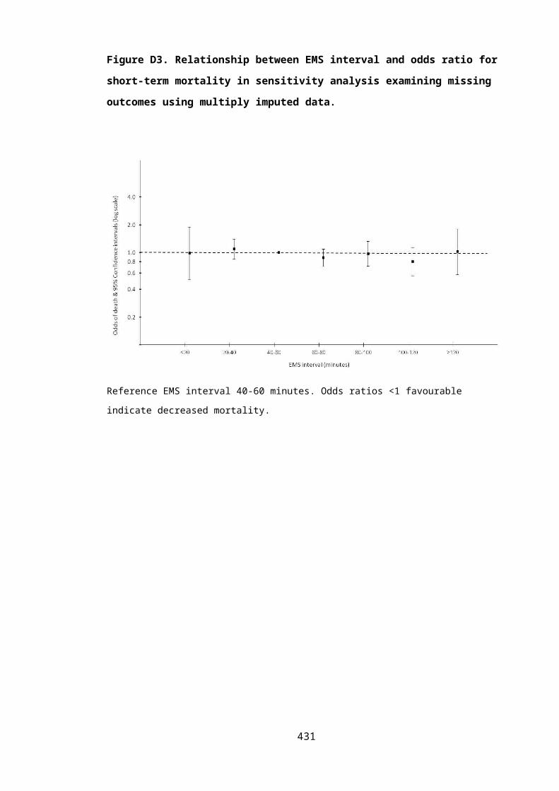
F.2.7 Systematic review of HSPWs for GOS categories: Statistical analyses

Health state preference weights were typically reported as a mean with either standard

deviation or standard error of the mean. To provide uniformity across results, estimates of

dispersion were converted into 95% confidence intervals using standard statistical formulae. [18]

To facilitate comparisons, extended GOS category HSPWs were combined using weighted

averages to provide results for commensurate basic GOS health states. Utility values within

each extended GOS category were assumed to be normally distributed and the basic GOS

category was assumed to divide equally with regards to severity to give upper and lower

categories of the extended score.

Variation in HSPWs between studies was examined with one way analyses of variance.

Published summary statistics were used to test for statistically significant differences between

HSPW estimates within each basic GOS category. A synthetic data set with the correct number

of cases, mean and standard deviation within each group was produced using the Stata

aovsum command. Post hoc Scheffe’s multiple comparison hypothesis tests for differences in

means were then used to identify which HSPW estimates differed. [19] This analysis requires that

assumptions of normally distributed utilities within each GOS category and equal variances are

not violated. Estimates from Djikers were based on a sample size of one and were excluded

from consideration. Where standard deviations/standard errors were not reported (and no

further information was available from the authors) it was assumed that the standard

deviation was equal to the mean utility value in each GOS category. A two-sided p-value of

<0.05 was considered to be statistically significant. Statistical analyses were performed in

STATA 12.1 (StataCorp, College Station, USA).

F.2.8 Adjusted limited dependent variable mixture modelling

Background

The distribution of EQ5D preference values has a number of distinctive features challenging

conventional approaches for statistical modelling. By definition, the maximum utility possible is

perfect health and EQ5D values are consequently constrained to be less than one. The

distribution is also limited at the lower end by a minimum possible value of -0.594 for the

worst possible health state (33333, representing extreme problems in all five EQ5D health

dimensions). The probability density function between these values is discontinuous,

multimodal and skewed. In most disease areas there is usually a large probability density at full

health. The next possible EQ5D value is 0.883 (the 11211 health state, corresponding to some

431

problems with usual activities) resulting in a large gap at the upper end of the distribution.

Although other smaller gaps exist across the possible range of EQ5D values, particularly at 0.45

as a result of the N3 term, the remainder of the distribution is usually considered to be

continuous. There are usually at least two modes located around EQ5D values of 0.2 and 0.7.

However, the exact number of modes, and their associated skewness and kurtosis, will vary

according to the patient characteristics and disease area being assessed. These distributional

characteristics normally remain after conditioning on patient or disease characteristics. [3, 20, 21]

A number of statistical approaches have been employed in mapping studies estimating EQ5D

HSPWs from clinical outcome scores or HRQOL measures. These have included linear

regression, generalised linear modelling, tobit regression, symmetrically trimmed least squares

regression, censored least absolute deviation (CLAD) models, adjusted limited dependent

variable models, response mapping, and 2 part logistic – linear regression models. [13, 22] Each of

these techniques have been shown to be sub-optimal with problems including prediction of

impossible values beyond the EQ5D range, under-prediction of high EQ5D values, and

systematic over-prediction at the lower end of the EQ5D scale. In response to these concerns a

novel modelling approach based on semi-parametric mixture models, the adjusted limited

dependent variable mixture model, has recently been developed and demonstrated to have

superior performance to previously used techniques.[20]

Mixture models can be used for two main purposes: identifying and describing heterogeneous

groups in a population; or to provide a semi-parametric framework to model challenging

distributions as in the current study.[23, 24] Mixture models combine a number of normal

distributions to produce extremely flexibly shaped distributions which can incorporate multi-

modality, and extreme kurtosis or skewness.[23, 24] Restricting these models, with a limited

dependent variable covering the range of possible EQ5D values, adjusting for the large

components of one’s, and rounding of predicted values above 0.883 to account for the gap

between full health and the next possible score, allows all important features of the EQ5D

distribution to be accounted for. The population is considered to be composed of several

distinct groups (often called latent classes, mixtures, classes, or components) which have

different distributions of EQ5D values. Mixture models determine the probability of latent

class membership using a multinomial logit model and then estimate a normal distribution for

each group. The relationship between patient characteristics and the probability of latent class

membership, and the form of each normal distribution, can be incorporated into the model.

The mean EQ5D is then calculated based on an average of the predictions from the normal

distribution for each latent class, weighted by the probabilities of component membership. [20]

432

Modelling strategy

The modelling strategy followed recommendations for mixture modelling and the

development of clinical prediction models.[20, 21, 25] As recommended by Hernandez (2014)

simple models were initially evaluated with the number of covariates and components

progressively increased.[26]

Two groups of models were developed. Previous TBI economic models have overwhelmingly

used cohort methodology, examining mixed male/female populations of a specified nominal

age.[27-32] Firstly, an initial model was therefore developed with 12 month EQ5D as the

dependent variable and GOS category and age as fixed explanatory variables. More complex

economic models, patient level simulations, or trial based economic evaluations may also

require HSPWs for GOS categories conditional on other patient characteristics. Age, gender,

co-morbidities, and the presence of extracranial injury were considered to represent

important patient variables likely to be important when characterising TBI populations, and

were therefore evaluated as further covariates in a second more detailed model. Previous

economic models have exclusively used basic GOS for defining health states and interest

therefore focused on the five level GOS version. Models for the eight level extended GOS were

developed in additional analyses.

Inclusion of explanatory variables was primarily determined by clinical considerations and all

specified covariates were judged to be important in influencing utility after TBI. Omission of

clearly non-significant variables (p>0.5) predicting utility in particular components, or the

probability of membership of specific components, was decided on an individual basis and

guided by measures of model goodness of fit. Polynomial terms were evaluated to account for

further non-linearity in the relationship between age and mean EQ5D. Coding of covariates is

summarised in Table F5. Secondary models examining extended GOS categories as dummy

variables did not converge, necessitating the use of a continuous term to predict latent class

membership. A quadratic term was evaluated to assess non-linearity but was non-significant.

The appropriate number of latent classes was determined by considering the proportion of

cases in each component, changes in information criterion statistics, and whether all important

parts of the EQ5D distribution were modelled. Higher BIC, emergence of very small

components likely to include only outlying data, and coverage of all important regions of the

EQ5D distribution argued against increased complexity.

433

Table F5. Coding of covariates in adjusted limited dependent variable mixture models

Explanatory

variable

Coding Rationale

Age Continuous linear term Categorisation would lose information.

Polynomial terms non-significant

Comorbidity Categorical:

No/ mildly limiting

Limiting /critical

Clinically meaningful categories within

constraints of data

Extracranial injury Categorical:

No non-head injury AIS≥3

Non-head injury AIS≥3

Clinically meaningful categories

Gender Male/female Natural categorisation

Basic GOS Categorical:

Vegetative state

Severe disability

Moderate disability

Good recovery

Death has a utility of zero and therefore does not

need to be predicted.

Extended GOS Categorical to predict mean

EQ5D within latent class

Continuous linear term to

predict latent class

membership

Non-convergence of model if extended GOS

entered as categorical variable to predict latent

class membership. Polynomial terms non-

significant

The parameters of mixture models are estimated using maximum likelihood with an

expectation maximisation algorithm. From an initial set of speculative starting values a

probability distribution for possible component memberships (or ‘completions’) is computed

using the current parameters. New parameters are then determined based on the current

completions, with the estimated model slightly improving. After a number of iterations the

algorithm converges to maximise the expected log-likelihood of the data.[33] A well known

problem is that the maximum likelihood estimation is very sensitive to the initial values and

can become trapped at local maxima in the likelihood function, meaning that the model’s

estimated parameters are not correct. To ensure a consistent solution was achieved, with the

maximum possible likelihood function, a number of steps were taken: Initial starting values

434

were varied, a constant only model was fitted and these starting values used to develop

subsequent models, and simulated annealing was implemented to identify the most

appropriate staring values.[21, 26, 34]

Goodness of model fit was evaluated using the Bayesian and Akaike’s information criterion

statistics, root mean squared error, and visual comparison of predicted and observed values

across the range of GOS categories. Adjusted limited dependent variable mixture modelling

was implemented using the aldmm module in Stata 12.1, using the siman module for

simulated annealing.[26]

435

F.3 ADDITIONAL RESULTS

F.3.1 Systematic review of HSPWs for GOS categories: ‘Near miss’ potentially eligible studies

Table F6. ‘Near miss’ potentially eligible studies identified during HSPW systematic reviewStudy Design TBI population Interventions Setting Dates n= Assessment

timeGlasgow Outcome Scale Version

Health state measurement

Notes

Ahmadi 2010[35]

Cohort study Severe TBI following decompressive craniectomy

n/a Germany 1997-2005 131 1 year Basic GOS SF-36

Andelic 2010[36]

Cohort study Moderate and severe TBI n/a Norway 1995-1996 62 10 years Extended GOS

SF-36

Bayen 2012[37]

Cohort study Severe TBI n/a France 2005 66 1 year Extended GOS

SF-36

Bell 2005[38] Randomised controlled trial

TBI undergoing rehabilitation Telephone follow up USA 1999-2001 180 1 year Extended GOS

EQ5DSF-36

Bell 2011[39] Randomised controlled trial

Moderate-severe TBI undergoing rehabilitation

Scheduled telephone intervention

USA 2005-2008 433 1 year Extended GOS

EQ5DSF-12

Blair 2010[40] Cohort study TBI undergoing rehabilitation n/a UK 2000-2007 28 1-10 years Extended GOS

SF-36

Boserelle 2010[41]

Cohort study Severe TBI n/a France 2004 518 1 year Extended GOS

EQ5D

Coplin 2001[42]

Randomised controlled trial

Severe TBI with raised ICP Decompressive craniectomy

USA NR 92 6 months Basic GOS SF-36

436

Study Design TBI population Interventions Setting Dates n= Assessment time

Glasgow Outcome Scale Version


Notes

Corteen 2012[43]


Severe TBI with refractory raised ICP Decompressive craniotomyMedical ICP management

UK Ongoing n/a 6 months Basic GOS SF-36 Ongoing RESCUE ICP trial

Davanzo 2008[44]

Cross sectional study

TBI (not further specified) n/a USA NR 60 NR Extended GOS

SF-36 PhD thesis, only abstract available.

Dikman 2003[45]

Cohort study Moderate and severe TBI at high risk of post-traumatic seizures

n/a USA 1991-1994 210 3- 5 years Basic GOS SF-36

Dimopolou 2004[46]

Cohort study Multiple trauma (including head injury)

n/a Greece 1999-2000 87 1 year Basic GOS Rosser disability scale

Gabbe 2010[47]

Cohort study TBI with: death after injury; an Injury Severity Score >15; an intensive care unit stay >24 hours requiring mechanical ventilation; and urgent surgery.

n/a Australia Ongoing n/a 6 months Basic GOS EQ5DSF-12

Guilfoyle 2010[48]

Cohort study TBI patients attending neurotrauma outpatients with GOSE 3-8

n/a UK NR 514 1-2 years Extended GOS

SF-36

Harrison 2013[49]

Cohort study TBI patients with initial GCS<15 requiring critical care

n/a UK 2008-2009 3,210 6 months Extended GOS

EQ5D

Hawthorne 2009[50]


TBI with EGOS>3. n/a Australia NR 66 3 months-15 years

Extended GOS

SF-36SF-6DAQoL

Hawthorne 2011[51]


TBI with EGOS>3. n/a Australia NR 66 3 months-15 years

Extended GOS

SF-36SF-6DAQoL

Unclear if different sample from Hawthorne 2009

437




Notes

Heijenbrok-kal 2009[52]

Cohort study Moderate and severe TBII n/a Netherlands 1999-2005 113 3 years Basic GOS SF-36

Holte 2012[53] Cohort study NR n/a Norway NR NR 1 year Extended GOS

EQ5D

Holtslag 2007[54]

Cohort study TBI with injury severity score >15 n/a Netherlands 1999-2000 181 1 year Basic GOS EQ5D

Intiso 2011[55] Cohort study Severe TBI following decompressive craniectomy

n/a Italy 2003-2007 70 1 year Basic GOS SF-36

Ksibi 2010[56] Cross sectional study

NR n/a Tunisia 2006 60 1 year Basic GOS SF-36 Translated from French

Lecky 2013[57] Cluster randomised trial

External signs of head injury, prehospital GCS<13, stable field vital signs.

Prehospital triage and bypassCurrent care

UK 2012-2013 262 6 months Extended GOS

EQ5D

Malmivaari 2009[58]

Cohort study TBI patients discharged from ICU requiring ventilator support

n/a Finland 2000-2003 176 1,2 & 5 years Extended GOS

SF-12DEQ5D

Malmivaari 2011[59]

Cohort study Severe TBI following decompressive craniectomy

n/a Finland 2000-2006 54 1 year Basic GOS EQ5D

McMillan 2013[60]

Cohort study TBI patients admitted to hospital for>24 hours

n/a UK NR 77 Discharge Extended GOS

SF-36

Nelson 2012[61]


Severe TBI Progesterone v current practice

Multicentre, international

Ongoing n/a 6 months Basic GOS SF-36 Ongoing SYNAPSE study

Ripley 2008[62]

Cohort study Female TBI patients requiring inpatient rehabilitation

n/a USA 2001-2005 30 1-3 years Extended GOS

SF-12

STITCH2010[63]


TBI with intracerebral haematomas Surgical or conservative management

UK 2010-2012 170 6 months Extended GOS

EQ5D Trial stopped due to poor recruitment

438




Notes

Temkin 2003[64]

Cohort study Moderate-severe TBI at high risk of post-traumatic seizures

n/a USA 1991-1994 209 3-5 years Basic GOS SF-36

Timofeev 2006[65]

Cohort study TBI patients undergoing decompressive craniectomy

n/s UK 2000-2003 49 6 months Basic GOS SF-36

Tomberg 2005[66]

Cohort study Moderate and severe TBI n/a Estonia 1996-1998 85 1-3 years Basic GOS SF-36

Townend 2001[67]

Cohort study Isolated mild to severe TBI n/a UK NR 121 1 month Extended GOS

EQ5D

Ulfarsson 2013[68]

Cohort study TBI with post-traumatic hypopituitarism

n/a Sweden 1999-2001 51 2-10 years Extended GOS

SF-36

Van Baalen 2006[69]

Cohort study Moderate and severe TBI n/a Netherlands NR 25 Hospital discharge and 1 year

Basic GOSExtended GOS

SF-36

Van Baalen 2010[70]

Cohort study Moderate and severe TBI n/a Netherlands NR 126 1 year Basic GOS SF-36

Von Elm 2008[71]

Cohort study Severe TBI n/a Switzerland 2005 101 6 months Extended GOS

SF-12

Von Steinbuchel 2010[72]


Mild to severe TBI with GOSE>2 n/a Netherlands, UK, Finland, France, Germany, Italy

NR 795 3 months to 15 years

Extended GOS

SF-36

Wilson 2000[73]`

Cohort study TBI admitted to specialist neuroscience centre

n/a UK NR 135 6 months Basic GOSExtended GOS

SF-36

Zeckey 2011[74]

Cohort study Multiple trauma patients with moderate and severe TBI

n/a Germany 1973-1990 620 10-23 years Basic GOS SF-12

439




Notes

F.3.2 Detailed risk of bias assessments for included GOS HSPW studies

Table F7. Risk of bias assessment for Kosty 2012 study

Kosty 2012[75]


Risk of bias

domain:


(Representative population

describing health states?)



measurement of health states?)



valuing health states?):


(Accurate and reproducible valuation

of preference for health states?):

Domain 5: Other

sources of bias:

Bias judgement:

Not applicable Low risk High risk Low risk Low risk

Support for judgement:

Health states measured using scenarios

Well designed health state descriptions meeting consensus standards.

GOS category for Good Recovery Upper assigned perfect health.

Relevant functional dimensions of GOS categories included.

Target population providing preferences was the USA general population.

The study sample comprised a non-representative sample of the general population.

50% of sample was young

Direct valuation method using standard gamble performed appropriately.

Structured interviews use to obtain preferences. Full details on methods not described e.g. use of props or training exercises.

No other sources of bias identified likely to influence results.

440

Heterogeneity of GOS states not fully accounted for e.g. Moderate disability addresses limitations in work only.

adults attending college. GOS category for Good Recovery Upper assigned perfect health.

Table F8. Risk of bias assessment for Smits 2010 study

Smits 2010[29, 76]


Domain: Domain 1: Selection bias






states?)




Domain 4: Information bias (Accurate and

reproducible valuation of preference for

health states?):

Domain 5: Other

sources of bias:

Bias judgement:

High risk Low risk Low risk Low risk Low risk


Target population for measuring health states was a sample of consecutive patients with complicated mild TBI.

Substantial loss to follow up for measurement using EQ5D (68%).

Validated preference based multiattribute health description instrument used with adequate coverage for GOS states – EQ5D.

Telephone interviews used to measure health states. Full details on methods not described e.g. structured

Health states valued by a sample of Dutch population representative of the target Dutch general population.

Preferences obtained indirectly using Dutch EQ5D tariff; derived from study meeting methodological standards for obtaining Preferences obtained indirectly using Dutch EQ5D tariff an algorithm for preferences.


441

Differences in case mix between included and excluded patients in terms of gender, age and TBI pathology.

interviews.

Table F9. Risk of bias assessment for Djikers 2004 study

Djikers 2004[77]


Risk of bias

domain:












valuation of preference for health

states?):

Domain 5: Other

sources of bias:

Bias judgement:

Not applicable High risk High risk Low risk Low risk



Rudimentary health states based on expert opinion.

Relevant functional dimensions of GOS categories included.

Target population providing preferences is health professionals.

The study sample comprised the study author only.

Preferences obtained indirectly using HUI-3 and QWB scoring algorithms.


442

Table F10. Risk of bias assessment for Tsauo 1999 study

Tsauo 1999[78]


Risk of bias

domain:




Domain 2: Information bias (Accurate

and reproducible measurement of

health states?)





bias (Accurate and

reproducible valuation of

preference for health

states?):

Domain 5: Other

sources of bias:

Bias judgement:

High risk High risk Unclear Unclear Low risk


Target population for measuring health states was patients with head injury following motorcycle accidents.

Study sample suffered from substantial loss to follow up (72%) with risk of selection bias if unrepresentative patients described

Patients asked to describe health state several years previously with concomitant risk of recall bias.

Untested translation of preference based multi-attribute health description instrument used with adequate coverage for GOS states (Rosser Index of health related quality of life).

Population valuing health states in the Rosser Index of health related quality of life not reported.

Direct valuation method using standard gamble.

Details of valuation exercises not published.


443

health statesTelephone interviews used to measure health states. Full details on methods not described e.g. structured interviews.

Table F11. Risk of bias assessment for Aoki 1998 study

Aoki 1998[79]


Domain: Domain 1: Selection bias











valuation of preference for health

states?):

Domain 5: Other

sources of bias:

Bias judgement:

Not applicable High risk Unclear Low risk Low risk



Health state descriptions do not meet consensus methodological standards.

Brief health state descriptions which don’t include all relevant functional dimensions of GOS categories.

Heterogeneity of GOS states not accounted for e.g. Moderate

Target population is Japanese health professionals.

Insufficient information reported on inclusion criteria and sample selection to allow assessment.

Direct valuation method using standard gamble performed appropriately.

Structured interviews use to obtain preferences. Full details on methods not described e.g. use of props or training exercises.


444

disability doesn’t address limitations in leisure activities

F.3.3 Covariance matrix of predictive model for mean 12 month EQ5D including basic GOS category and patient age

Table F12. Covariance matrix for initial model including basic GOS and age

Explanatory variables within component 1 Explanatory variables within component 2

Explanatory variables within component 3

Explanatory variables explaining the probability of component 1

membership

Explanatory variables explaining the probability of component 2

membershipVS SD MD Age Con

sVS SD MD Age Con

sVS SD MD Age Con

sVS SD MD Age Con

sVS SD MD Age Con

sExplanatory variables within component 1

VS 0.02137

SD 0.00195

0.00341

MD 0.00238

0.00175 0.02167

Age 0.00001

-0.00002 0.00001

0.00000

Cons -0.00286

-0.00110 -0.002

74

-0.000

05

0.00513


VS 0.00057 -0.00010

0.00005

0.00000

-0.000

14

0.02741

SD -0.00003 -0.00001

-0.000

03

0.00000

-0.000

02

0.00070

0.00074

MD -0.00001 -0.00003

0.00015

0.00000

-0.000

03

0.00070

0.00069

0.00072

Age 0.00000 0.00 0.000 0.000 0.000 0.000 0.000 0.000 0.000

445

000 00 00 00 00 00 00 00Cons 0.00002 0.00

002-

0.00005

0.00000

0.00005

-0.000

68

-0.000

67

-0.000

72

0.00000

0.00080


VS 0.00000

0.00000 0.00000

0.00000

0.00000

0.00000

0.00000

0.00000

0.00000

0.00000

0.00000

SD 0.00013

0.00009 0.00048

-0.000

02

0.00062

-0.000

35

-0.000

44

-0.000

41

0.00000

0.00039

0.00000

0.00136

MD 0.00013

-0.00011 -0.000

68

0.00000

-0.000

19

-0.000

43

-0.000

44

-0.000

43

0.00000

0.00041

0.00000

0.00053

0.00096

Age 0.00000

-0.00001 0.00002

0.00000

0.00000

0.00000

0.00000

0.00000

0.00000

0.00000

0.00000

0.00001

0.00001

0.00000

Cons -0.00021

0.00041 -0.001

48

0.00000

0.00017

0.00039

0.00047

0.00038

0.00000

-0.000

32

0.00000

-0.000

91

-0.001

01

-0.000

02

0.00215

Explanatory variables explaining the probability of component 1 membership

VS 0.00004 -0.00009 -0.000

14

0.00000

-0.000

20

0.00003

0.00002

0.00002

0.00000

-0.000

02

0.00000

-0.000

12

-0.000

01

0.00000

0.00003

0.00006

SD 0.00048 0.00352 0.02059

-0.000

21

0.00907

0.00246

0.00080

0.00476

0.00008

-0.006

51

0.00000

0.01146

-0.005

11

0.00012

-0.016

28

-0.000

66

1.51204

MD 0.00054 0.01268 0.00442

-0.000

26

0.01042

0.00008

0.00036

0.00098

0.00002

-0.001

83

0.00000

0.00706

0.00180

0.00003

-0.005

25

-0.001

14

0.24522

0.26766

Age 0.06782 -0.00044 0.01209

0.00003

-0.006

32

0.03398

0.00015

0.00094

0.00001

-0.001

51

0.00000

0.00474

0.00461

0.00012

-0.011

44

-0.000

06

0.17562

0.08822

253940.67000

Cons

-0.00633 0.00321 -0.005

02

-0.000

19

0.01238

-0.002

40

-0.001

10

-0.001

83

-0.000

02

0.00261

0.00000

0.00049

-0.003

93

-0.000

12

0.00958

-0.002

55

-0.148

13

-0.049

02

-0.12817 0.23255


VS 0.00002 -0.00004 -0.000

10

0.00000

-0.000

07

0.00002

0.00001

0.00001

0.00000

-0.000

01

0.00000

-0.000

04

0.00000

0.00000

0.00002

0.00003

-0.000

88

-0.000

52

-0.00011 -0.001

02

0.00002

SD 0.00307 -0.00452 0.02093

-0.000

06

-0.000

15

0.00270

0.00117

0.00375

0.00006

-0.005

84

0.00000

0.01329

0.01126

0.00034

-0.032

29

-0.000

72

0.61324

0.20068

0.26339 -0.228

11

-0.000

43

0.81215

MD 0.00178 0.00127 0.02224

-0.000

16

0.00514

0.00206

0.00107

0.00334

0.00005

-0.005

43

0.00000

0.01336

0.01079

0.00030

-0.028

83

-0.001

05

0.48636

0.27500

0.23937 -0.194

19

-0.000

69

0.73301

0.73537

Age -0.21802 0.00255 0.02693

-0.000

34

0.01477

-0.113

06

0.00068

0.00275

0.00005

-0.004

68

0.00000

0.01580

0.01246

0.00032

-0.031

32

-0.003

27

0.46356

0.25944

253938.31000

-0.102

77

-0.001

26

0.77011

0.74337

253947.49000

Cons -0.00419 0.00643 -0.021

25

-0.000

03

0.00512

-0.003

22

-0.001

62

-0.003

67

-0.000

04

0.00549

0.00000

-0.010

52

-0.012

30

-0.000

34

0.03089

-0.000

38

-0.390

78

-0.157

61

-0.25220 0.26579

-0.000

36

-0.737

44

-0.670

05

-0.68930 0.73211

446

F.3.4 Formula to predict mean 12 month EQ5D from adjusted limited dependent variable

mixture model

Where:

E=conditional expectation

yi= EQ5D value

xi’=Vector of covariates

wi’=Vector of variables affecting latent class membership

δc=Vector of coefficients corresponding to vector of variables affecting latent class

membership

C= Number of latent classes used in the analysis

s,c=Individual latent classes

∅ (.)=Standard normal density function

φ(.)=Standard cumulative normal function

ψ1=0.0883

ψ2=-0.594

447

F.3.5 Predictive model for mean 12 month EQ5D including basic GOS category and patient

characteristics of age, gender, extracranial injury and co-morbidity

Table F13. Model coefficients for detailed model including basic GOS, age, gender,

extracranial injury and co-morbidity

Variable* Coefficient SE p-Value 95% Confidence

Interval


Moderate disability 0.716 83.529 0.993 -162.999 164.431

Good recovery 1.153 0.079 0.000 0.998 1.307

Age 0.002 0.002 0.314 -0.002 0.005

Female gender -0.149 0.066 0.023 -0.277 -0.020

Limiting or critical co-morbidity -0.342 0.114 0.003 -0.566 -0.118

Major extracranial injury -0.085 0.054 0.117 -0.191 0.021

Constant 0.021 0.092 0.816 -0.159 0.201


Moderate disability 0.074 0.009 0.000 0.057 0.091

Good recovery 0.169 0.012 0.000 0.146 0.191

Age -0.001 0.000 0.000 -0.001 -0.001

Female gender -0.019 0.007 0.008 -0.033 -0.005

Limiting or critical co-morbidity -0.006 0.008 0.439 -0.023 0.010

Major extracranial injury -0.036 0.007 0.000 -0.050 -0.023

Constant 0.765 0.013 0.000 0.739 0.791



Good recovery 0.064 0.044 0.149 -0.023 0.151

Age -0.001 0.001 0.014 -0.002 0.000

Female gender -0.027 0.020 0.160 -0.066 0.011

Limiting or critical co-morbidity 0.006 0.024 0.794 -0.040 0.053


Constant 0.229 0.047 0.000 0.137 0.321


Moderate disability -0.023 0.007 0.002 -0.037 -0.008

Good recovery -13.597 580.960 0.981 -1152.258 1125.063

Age 3.549 0.627 0.000 2.321 4.777

Female gender -0.448 0.441 0.310 -1.312 0.416

Limiting or critical co-morbidity -1.063 0.542 0.050 -2.126 0.000

Extracranial injury 0.413 0.320 0.197 -0.214 1.041448

Constant 0.618 0.618 0.317 -0.593 1.830



Good recovery 1.108 0.196 0.000 0.724 1.493

Age 3.119 0.303 0.000 2.525 3.712

Female gender -0.173 0.132 0.191 -0.431 0.086

Limiting or critical co-morbidity -0.404 0.147 0.006 -0.693 -0.115

Extracranial injury 0.169 0.135 0.211 -0.096 0.434

Constant 0.197 0.290 0.498 -0.373 0.766

*Basic GOS coded as indicator variable with GOS 3, severe disability, as the baseline category. Basic GOS

category 1, death, not modelled as this will equal zero by definition. Vegetative state excluded due to

model instability/lack of convergence secondary to low number of patients in this GOS category.

Covariance matrix available from author on request.

449

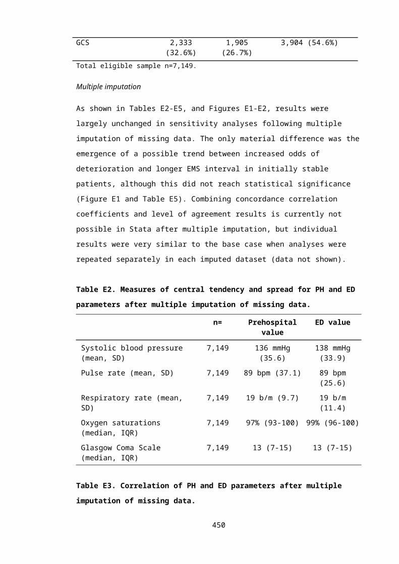
F.3.6 Predictive model for mean 12 month EQ5D including extended GOS category and age

Table F14. Model coefficients for secondary initial model including extended GOS and age

Variable* Coefficient SE p-Value

95% Confidence Interval

Explanatory variables within component 1*Vegetative state -0.566 0.166 0.001 -0.892 -0.239Lower SD -0.446 0.094 0.000 -0.630 -0.263Upper SD 0.169 0.109 0.122 -0.045 0.382Lower MD 0.263 0.130 0.044 0.007 0.519Upper MD -0.110 0.093 0.240 -0.292 0.073Lower GR -0.133 0.099 0.177 -0.327 0.060Age 0.247 0.099 0.013 0.053 0.442Constant -0.566 0.166 0.001 -0.892 -0.239Explanatory variables within component 2*

Vegetative state -1.284 0.178 0.000 -1.632 -0.936Lower SD -0.242 0.013 0.000 -0.267 -0.217Upper SD -0.225 0.019 0.000 -0.262 -0.187Lower MD -0.193 0.013 0.000 -0.218 -0.168Upper MD -0.157 0.014 0.000 -0.184 -0.130Lower GR -0.090 0.014 0.000 -0.118 -0.062Age 0.995 0.013 0.000 0.970 1.020Constant -1.284 0.178 0.000 -1.632 -0.936Explanatory variables within component 3*

Vegetative state -1.436 2.209 0.516 -5.767 2.894Lower SD -1.180 2.201 0.592 -5.493 3.133Upper SD -1.316 2.200 0.550 -5.627 2.995Lower MD -1.267 2.199 0.564 -5.578 3.043Upper MD -0.606 2.200 0.783 -4.918 3.706Lower GR -0.453 2.199 0.837 -4.764 3.857Age 1.437 2.198 0.513 -2.870 5.744Constant -1.436 2.209 0.516 -5.767 2.894Explanatory variables explaining the probability of component 1 membership

Extended GOS* -0.373 0.152 0.014 -0.671 -0.075Age 0.010 0.006 0.075 -0.001 0.021Constant 0.983 0.819 0.230 -0.623 2.589Explanatory variables explaining the probability of component 2 membership

Extended GOS* 0.290 0.141 0.039 0.014 0.566Age 0.011 0.004 0.002 0.004 0.019Constant -1.014 0.662 0.125 -2.311 0.282

*Extended GOS coded as indicator variable with GOS 8, upper good recovery, as the baseline category.

**Extended GOS included as continuous numeric variable to predict component membership. Covariance matrix available from

author on request.

450

F.3.7 Predictive model for mean 12 month EQ5D including extended GOS category and

patient characteristics of age, gender, extracranial injury and co-morbidity

Table F15. Model coefficients for secondary detailed model including extended GOS, age,

gender, extracranial injury and co-morbidity

Variable* Coefficient SE p-

Value



Lower SD -0.206 0.101 0.043 -0.404 -0.007

Upper SD -0.151 0.104 0.146 -0.354 0.052

Lower MD -0.104 0.102 0.312 -0.304 0.097

Upper MD -0.003 0.104 0.975 -0.208 0.201

Lower GR -0.040 0.114 0.724 -0.263 0.183

Age 0.000 0.001 0.737 -0.001 0.001

Female gender -0.026 0.020 0.187 -0.066 0.013

Serious co-morbidity -0.002 0.022 0.931 -0.045 0.041


Constant 0.303 0.103 0.003 0.102 0.505


Lower SD -0.233 0.012 0.000 -0.257 -0.210

Upper SD -0.227 0.013 0.000 -0.252 -0.202

Lower MD -0.181 0.011 0.000 -0.203 -0.160

Upper MD -0.154 0.009 0.000 -0.172 -0.136

Lower GR -0.087 0.009 0.000 -0.105 -0.069

Age -0.001 0.000 0.000 -0.001 -0.001

Female gender -0.023 0.007 0.000 -0.036 -0.010

Serious co-morbidity -0.026 0.007 0.000 -0.040 -0.012


Constant 1.016 0.010 0.000 0.996 1.037


Lower SD -0.550 0.011 0.000 -0.571 -0.529

Upper SD -0.619 0.015 0.000 -0.649 -0.589

Lower MD -0.509 0.016 0.000 -0.540 -0.478

Upper MD -0.478 0.014 0.000 -0.506 -0.451

Lower GR -0.446 0.012 0.000 -0.469 -0.423

Age -0.002 0.000 0.000 -0.003 -0.002

Female gender 0.006 0.008 0.425 -0.009 0.021


Major extracranial injury 0.015 0.008 0.061 -0.001 0.031

Constant 1.234 0.019 0.000 1.198 1.271


451

Lower SD 4.788 0.727 0.000 3.363 6.212

Upper SD 4.603 0.927 0.000 2.787 6.420

Lower MD 3.797 0.778 0.000 2.272 5.322

Upper MD 2.984 0.781 0.000 1.454 4.514

Lower GR 2.233 0.807 0.006 0.652 3.815

Age -0.008 0.010 0.429 -0.029 0.012

Female gender -0.564 0.379 0.136 -1.307 0.178


Serious co-morbidity 0.627 0.459 0.172 -0.273 1.526

Constant -1.581 0.924 0.087 -3.393 0.230


Lower SD -0.348 0.606 0.566 -1.536 0.840

Upper SD 0.599 0.827 0.469 -1.022 2.221

Lower MD -0.019 0.677 0.978 -1.346 1.309

Upper MD 0.433 0.666 0.516 -0.872 1.737

Lower GR 0.813 0.650 0.211 -0.461 2.087

Age 0.002 0.010 0.852 -0.019 0.023

Female gender -0.661 0.373 0.077 -1.393 0.071


Serious co-morbidity 0.528 0.429 0.218 -0.313 1.369

Constant 2.536 0.859 0.003 0.853 4.219

Extended GOS coded as indicator variable with GOS 8, upper good recovery, as the baseline category.

Extended GOS category 1, death, not modelled as this will equal zero by definition. Vegetative state

excluded due to model instability/lack of convergence secondary to low number of patients in this GOS

category. Covariance matrix available from author on request.

452

F.3.8 Predictive model for mean 12 month EQ5D including basic GOS category (excluding

vegetative state) and age

Table F16. Model coefficients for initial model including basic GOS (vegetative state

excluded) and age


Value

95% Confidence

Interval


Severe disability 0.134 0.022 0.000 0.090 0.178


Age 0.000 0.000 0.699 -0.001 0.001

Constant 0.078 0.030 0.008 0.020 0.136




Age 0.000 0.000 0.551 0.000 0.000

Constant 0.857 0.013 0.000 0.832 0.882




Age -0.001 0.000 0.000 -0.001 0.000

Constant 0.695 0.017 0.000 0.661 0.728


Severe disability -0.008 0.003 0.005 -0.013 -0.002


Age -3.206 0.229 0.000 -3.656 -2.756

Constant 0.725 0.202 0.000 0.329 1.121




Age 1.192 0.234 0.000 0.733 1.652

Constant -0.505 0.344 0.142 -1.179 0.169

Basic GOS coded as indicator variable with GOS 5, good recovery, as the baseline category. Basic GOS

category 1, death, not modelled as this will equal zero by definition. Vegetative state excluded.

Covariance matrix available from author on request.

453

F.3.9 Predictive model for mean 12 month EQ5D including basic GOS category (combining

vegetative state and severe disability) and age

Table F17. Model coefficients for initial model including basic GOS (vegetative state/severe

disability combined)


Value

95% Confidence

Interval


Vegetative state/ Severe disability -0.272 0.059 0.000 -0.387 -0.158


Age 0.003 0.001 0.005 0.001 0.005

Constant 0.108 0.072 0.135 -0.034 0.250




Age -0.001 0.000 0.000 -0.001 0.000

Constant 0.917 0.028 0.000 0.862 0.972




Age -0.002 0.001 0.000 -0.004 -0.001

Constant 1.063 0.046 0.000 0.974 1.153


Vegetative state/ Severe disability 0.005 0.008 0.495 -0.010 0.020


Age 1.718 1.258 0.172 -0.748 4.184

Constant -3.481 0.477 0.000 -4.415 -2.546


Vegetative state/ Severe disability 0.007 0.004 0.078 -0.001 0.015


Age 2.461 0.888 0.006 0.720 4.202

Constant -1.066 0.843 0.206 -2.718 0.587

Covariance matrix available from author on request. Basic GOS coded as indicator variable with GOS 3,

severe disability, as the baseline category. Basic GOS category 1, death, not modelled as this will equal

zero by definition.

454

F.3.10 Effect of initial injury severity on mean EQ5D values for GOS categories

To explore the possibility that initial injury severity influences utility values for a given 12

month GOS health state two additional secondary analyses were performed. Firstly, predicted

mean EQ5D values from the simple adjusted limited dependent variable mixture model

(ALDVMM, including age and basic GOS category only) were compared between patients with

and without major trauma, defined as ISS>15. Linear regression of an identically specified

model was additionally performed to aid interpretation of results. Secondly, ISS was specified

as an additional predictor in the detailed predictive ALDVMM, together with basic GOS

category, age, comorbidity, gender and extra-cranial injury. Again linear regression was also

performed to allow more transparent interpretation of model coefficients.

Replicating GOS to EQ-5D mapping for the simple predictive model in patients with and

without major trauma demonstrated that there was no statistically significant difference in

utility according to the presence of major trauma (non-significant component and latent class

coefficients in ALDVM model, major trauma linear regression coefficient p=0.34). However the

relatively imprecise 95% confidence intervals were potentially consistent with a small but

clinically significant difference in utility between patients presenting with and without major

trauma, as shown in Figure F1.

Importantly, ISS was not a significant independent predictor of utility when included in the

detailed model with extracranial injury (non-significant component and latent class coefficients

in ALDVM model, ISS linear regression coefficient p=0.36), suggesting that disability arising

from non-head injuries is influential, rather than the overall severity of the intial injury.

Taken together these results indicate that a patient’s mean 12 month EQ5D is determined by

their global disability level after treatement and recovery, rather than the presence of major

trauma per se. This is perhaps unsurprising as GOS is designed as a stand alone outcome

measure regardless of the magnitude of the intial insult; and HRQOL would be expected to

decrease in the presence of pain, depression and anxiety caused by non-head injuries, but

which are not fully assessed in the GOS. 455

Figure F1. Mean predicted 12 month EQ5D for each basic GOS category in patients with and

without major trauma

Symbols represent point estimates from the initial adjusted limited dependent variable mixture model

for predicted mean EQ5D values for different subgroups of patients aged 50 years (: presented without

major trauma, :presented with major trauma :All patients) and basic GOS category (D:dead, VS:

Vegetative state, SD: Severe disability, MD: Moderate disability, GR: Good recovery) . Error bars report

95% confidence interval for predicted mean. Note, no patients in vegetative state observed within the

subgroup without major trauma.

456

F.3.11 Mean EQ5D values for basic GOS categories based on non-UK preference tariffs

Table F18. Mean EQ5D values for basic GOS categories using a range of international

preference tariffs

Glasgow Outcome Scale category: Mean (sd)

GOS 1:Death

GOS 2:Vegetative

state

GOS 3:Severe

disability

GOS 4:Moderate disability

GOS 5:Good

recoveryn= - 6 900 1,222 1,309

United Kingdom 0

(-)

-0.178

(0.19)

0.382

(0.35)

0.675

(0.27)

0.894

(0.16)

Denmark 0

(-)

-0.478

(0.20)

0.489

(0.29)

0.711

(0.20)

0.900

(0.14)

Germany 0

(-)

0.327

(0.14)

0.555

(0.30)

0.811

(0.22)

0.946

(0.11)

Netherlands 0

(-)

0.125

(0.18)

0.471

(0.29)

0.696

(0.25)

0.905

(0.15)

Spain 0

(-)

-0.397

(0.13)

0.350

(0.39)

0.718

(0.25)

0.917

(0.14)

Japan 0

(-)

0.072

(0.10)

0.529

(0.20)

0.710

(0.14)

0.884

(0.14)

United States 0

(-)

0.092

(0.96)

0.540

(0.24)

0.754

(0.17)

0.914

(0.12)

Zimbabwe 0

(-)

0.184

(0.15)

0.529

(0.20)

0.710

(0.14)

0.884

(0.14)

457

F.3.12 Mean EQ5D values for extended GOS categories based on non-UK preference tariffs

Table F19. Mean EQ5D values for extedended GOS categories using a range of international

preference tariffs

Glasgow Outcome Scale category:Mean (sd)

GOSE 1:Death

GOSE 2:Vegetative

state

GOSE 3:Lower severe

disability

GOSE 4:Upper severe

disability

GOSE 5:Lower

moderate disability

GOSE 6:Upper

moderate disability

GOSE 7:Lower good

recovery

GOSE 8:Upper good

recoveryn= - 6 616 284 498 724 564 745

United

Kingdom

0

(-)

-0.177

(0.19)

0.325

(0.35)

0.505

(0.31)

0.586

(0.30)

0.735

(0.22)

0.838

(0.18)

0.937

(0.12)

Denmark 0

(-)

-0.048

(0.20)

0.447

(0.30)

0.582

(0.23)

0.644

(0.23)

0.758

(0.16)

0.849

(0.15)

0.938

(0.11)

Germany 0

(-)

0.327

(0.14)

0.501

(0.30)

0.670

(0.27)

0.741

(0.26)

0.859

(0.17)

0.916

(0.14)

0.970

(0.08)

Netherland

s

0

(-)

0.125

(0.18)

0.432

(0.29)

0.555

(0.28)

0.614

(0.28)

0.754

(0.20)

0.854

(0.17)

0.944

(0.11)

Spain 0

(-)

-0.397

(0.13)

0.269

(0.40)

0.525

(0.30)

0.634

(0.28)

0.776

(0.20)

0.870

(0.16)

0.952

(0.10)

Japan 0

(-)

0.072

(0.10)

0.493

(0.21)

0.605

(0.15)

0.666

(0.14)

0.741

(0.138)

0.828

(0.15)

0.926

(0.12)

United

States

0

(-)

0.092

(0.10)

0.496

(0.25)

0.634

(0.20)

0.696

(0.20)

0.794

(0.14)

0.870

(0.13)

0.946

(0.10)

Zimbabwe 0

(-)

0.184

(0.150

0.522

(0.21)

0.641

(0.17)

0.707

(0.17)

0.792

(0.13)

0.866

(0.13)

0.945

(0.10)

GOSE: Extended Glasgow Outcome Scale

458

F.3.13 Victoria State Trauma Registry mapping study of GOS categories onto UK tariff EQ5D

index values: Missing data

There was a moderate proportion of missing data for important study variables, ranging from

0% for age and sex to 27.0% for 12 month EQ5D (Table F20). Case-wise missingness for the

initial predictive model (including age and GOS only) ranged from 72.8% of cases with no

missing data to 18.3% of patients missing data on both 12 month EQ5D and basic GOS. Case-

wise missingness for the detailed predictive model (including age, GOS, and other coavriates)

varied from 65.5% of cases having no missing data on any variable to 1.9% of cases missing

data on 3 out of the 6 included variables (Table F21).

Table F20. Missing data levels for variables included in models predicting 12 month EQ5D

Patient characteristic(Total sample size 4,719)

Data incompleteness*Cases with missing data, (%)

12 month EQ5D 1,275 (27.0%)

12 month GOS 870 (18.4%)

Age 0 (0%)

Gender 0 (0%)

Co-morbidity 480 (10.2%)

Extracranial injury 2 (0.04%)

Table F21. Missing data levels for variables included in models predicting 12 month EQ5D

Variables missing from initial model

Number of cases, (%)*

Variables missing from detailed model

Number of cases, (%)*

None 3,437 (72.8%) None 3,089 (65.5%)

GOS 7 (0.2%) EQ5D 370 (7.8%)

EQ5D 412 (8.7%) Co-morbidity 347 (7.4%)

EQ5D and GOS 863 (18.3%) EQ5D and GOS 773 (16.4%)

Co-morbidity and extracranial 1 (0.02%)

Co-morbidity and extracranial injury

1 (0.02%)

EQ5D and co-morbidity 42 (0.9%)

EQ5D, GOS, co-morbidity 89 (1.9%)

EQ5D, GOS, extracranial injury 1 (0.02%)

459

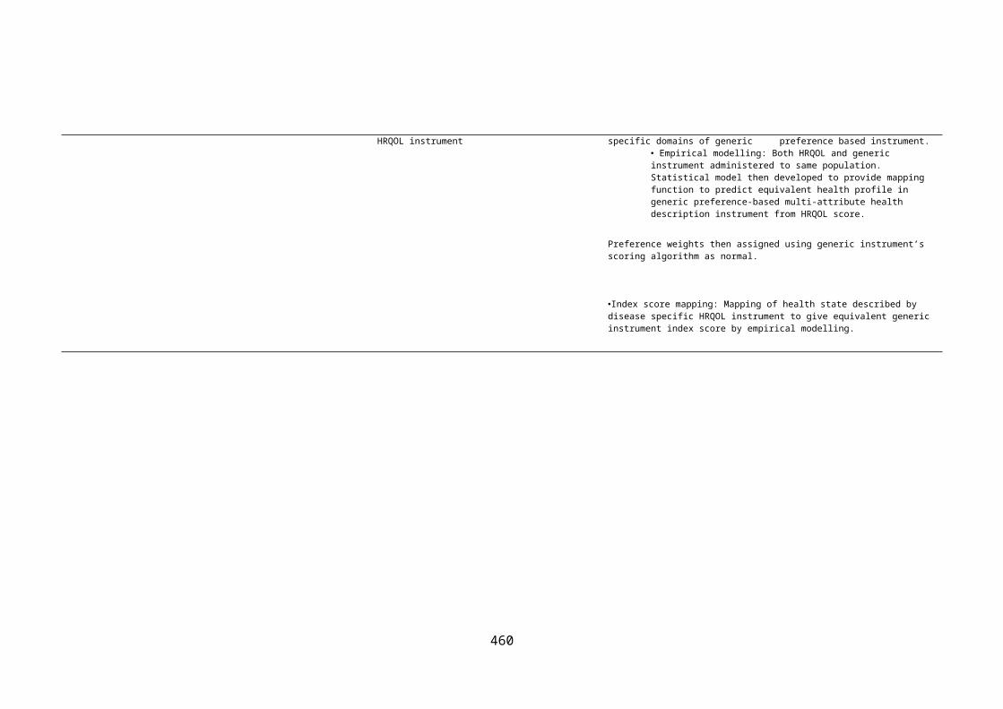
*Total sample size n=4,719

Patients excluded from the available case analyses due to missing data had broadly similar

characteristics to included patients, as detailed in Table F22. The only clinically and statistically

significant differences were that excluded patients were marginally younger with slightly less

severe injuries.

Table F22. Characteristics of included and excluded cases

Initial model Detailed modelPatient characteristic Included Excluded p-value Included Excluded p-

value

Number of patients 3,437 1,282 3,089 1,630

Age at injury(Years, median, IQR)

50(29-72)

45(27-67)

0.001 50(29-72)

46(28-67)

<0.001

Male gender (%, 95% CI)

71.3(69.8-72.9)

73.0(70.6-75.4)

0.26 70.8(69.2-72.4)

73.6(71.5-75.8)

0.04

Co-morbidities (%, 95% CI):

Limiting or critical systemic illness

27.1(25.5-28.7)

28.1(25.5-30.7)

n=1,150

0.52 27.1(25.5-28.7)

28.1(25.5-30.7)

0.52

Head region AIS (%, 95% CI):

AIS 3 37.0(35.4-38.7)

26.2(33.6-38.8)

0.53 36.9(35.2-38.6)

33.7(34.3-39.0)

0.37

AIS 4 40.4(38.7-42.0)

42.0(39.3-44.7)

40.6(38.9-42.4)

41.2(38.8-43.6)

AIS 5 22.5(21.1-23.9)

21.6(19.4-23.9)

22.5(21.0-23.9)

21.9(19.9-23.9)

AIS 6 - - - -

AIS 9† 0.05(0.0-0.01)

0.16(0.0-0.37)

0.03(0.0-0.09)

0.19(0.0-0.39)

Admission GCS(median, IQR)

14(13-15)

14(13-15)n=1,237

0.72 14(13-15)

14(13-15)n=1,566

0.002

Extracranial injury( AIS≥3, %, 95% CI)

30.8(29.3-32.4)

n=3,436

25.5(23.1-27.9)

n=1,281

<0.001 30.6(28.9-32.2)

27.1(25.0-29.3)

n=1,628

0.02

ISS(median,IQR)

21(16-26)

19(16-26)n=1,281

0.001 20(16-26)

20(16-26)n=1,628

0.05

12 month EQ5D(mean, 95% CI)

0.68(0.67-0.69)

0.71(0.30-1.0)

n=7

0.51 0.68(0.67-0.69)

0.68(0.65-0.72)

0.89

460

Identical principles to those previously described were used to develop multiple imputation

models and generate 5 simulated imputed datasets, under a missing at random assumption.

Variables included in the imputation models included EQ5D, all covariates used in the analysis

models, and the following auxiliary variables: injury severity score, head region AIS score,

discharge status, geographical location of injury, funding status of patient, mechanism of

injury, and date of injury. Unfortunately socioeconomic status and ethnicity variables were

unavailable. Predictive mean matching was used to account for non-normality in the EQ5D

distribution. Mean 12 month EQ5D conditional on basic GOS category and the initial predictive

model were then implemented in the imputed datasets with Rubin’s rules used to derive

appropriate parameter estimates as previously described. There were negligible differences in

mean EQ5D for each GOS categories (Table F23). Coefficients for the initial basic GOS model

were also minimally different except for greater precision for vegetative state parameters

(Table F24). Results for other secondary analyses were also not materially changed (data not

shown).

Table F23. Mean 12 month EQ5D conditional on basic GOS category compared between

available case and multiple imputation analyses.

Overall Stratified by basic GOS category

GOS 2:PVS

GOS 3:Severe

disability


GOS 5:Good

recoveryAvailable case 12 month EQ5D(mean, 95% CI, n=3,443)

0.68(0.67-0.69)

-0.178(-0.33- -

0.03)

0.382(0.36-0.41)

0.674(0.66-0.69)

0.894(0.89-0.90)

Imputed 12 month EQ5D(mean, 95% CI,n=4,717)

0.68(0.67-0.69)

-0.154(-0.32-0.01)

0.380(0.36-0.40)

0.673(0.66-0.69)

0.895(0.89-0.90)

461

Table F24. Coefficients for adjusted limited dependent variable mixture model predicting 12 month

EQ5D HSPWs from basic GOS category and age after multiple imputation.


Value

95% Confidence

Interval


Vegetative state 0.251 0.366 0.493 -0.466 0.967



Age 0.002 0.001 0.023 0.000 0.004

Constant 0.191 0.062 0.002 0.069 0.313


Vegetative state -0.090 0.175 0.607 -0.434 0.254



Age -0.001 0.000 0.000 -0.001 0.000

Constant 0.913 0.026 0.000 0.862 0.964


Vegetative state -1.136 0.038 0.000 -1.209 -1.062



Age -0.002 0.000 0.000 -0.003 -0.001

Constant 1.026 0.032 0.000 0.963 1.089


Vegetative state 0.226 1.211 0.852 -2.147 2.599



Age 0.006 0.006 0.327 -0.006 0.019

Constant -3.497 0.404 0.000 -4.289 -2.705


Vegetative state -2.805 2.045 0.170 -6.812 1.203



Age 0.005 0.003 0.172 -0.002 0.011

Constant -0.965 0.776 0.213 -2.486 0.555

*Basic GOS coded as indicator variable with GOS 5, good recovery, as the baseline category. Basic GOS

category 1, death, not modelled as this will equal zero by definition.

462

F.3.14 Change in mean EQ5D for basic GOS categories over time

Two thousand five hundred and forty seven patients, injured between 2009 and 2011, had

complete data on both GOS and EQ5D at 6, 12 and 24 months and were included in an

available case analysis examining change in mean utility values for GOS categories over time. A

generalised estimating equations model,[80] using an auto-regressive working correlation

structure and an interaction term for GOS (as a time varying covariate) and time, was used to

test whether the mean EQ5D preference weight for GOS categories significantly differed over

each time point. As shown in Table F25 mean EQ5D preference weights varied very slightly

across different measurement time points for each basic GOS category, but only differed to

statistically significant extent for the severe disability health state.

Table F25. Mean EQ5D preference weights for GOS categories at different time points post

TBI

Measurement time

Glasgow Outcome Scale category

GOS 1:Death

GOS 2:PVS

GOS 3:Severe

disability


GOS 5:Good

recovery

6 months 0

(-)

-0.120

(0.632)

0.379

(0.012)

0.669

(0.007)

0.879

(0.004)

EQ5D (mean, se)

12 months 0

(-)

-0.178

(0.078)

0.382

(0.012)

0.675

(0.008)

0.894

(0.004)

24 months 0

(-)

-0.069

(0.056)

0.392

(0.126)

0.646

(0.008)

0.904

(0.004)

Largest

difference

0 0.109 0.013 0.029 0.025

p-value* - 0.80 0.01 0.33 0.08

*p-value for null hypothesis of no difference in mean EQ5D for each GOS category across

measurement time points.

463

F.3.15 Linear regression models predicting mean 12 month EQ5D from GOS categories and

patient characteristics

Background and methods

An ordinary least squares prediction model was also developed to allow a comparison of the

performance of a simpler and more intuitive statistical approach to the adjusted limited

dependent variable mixture model. There is conflicting evidence regarding the validity of a

linear regression for mapping EQ5D index scores.[13] Concerns, arising secondary to the unusual

EQ5D distribution, include the likely violation of assumptions of normality and

homoscedasticity of error terms, the possibility of predictions outside the feasible range, and

under/over prediction of utility for extreme health states. However, in some settings linear

regression has appeared to outperform other commonly used modelling approaches (tobit,

limited dependent variable mixture models, or two part models) and shown reasonably

comparable results to the adjusted limited dependent variable model. [13, 21]

The modelling approach was informed by expert recommendations and followed the same

strategy as described previously.[81] Initial models considered basic GOS and age only, with

detailed models including basic GOS, age, co-morbidity, extracranial injury and gender. Non-

linearity between age and EQ5D index score was evaluated using polynomial terms. Inclusion

of explanatory variables was based on clinical theory, with covariate exclusion only considered

in the case of gross non-significance (p>0.5) and worsening model fit. Interactions between

basic GOS and each explanatory variable were initially assessed in a Wald ‘chunk’ test. [82] If this

was significant individual interactions were subsequently examined. Huber-White sandwich

estimates of variance were used to compute robust standard errors accounting for model

misspecification, non-normality of error terms or heteroscedasticity.[83, 84] Goodness of model

fit was assessed using R2, root mean squared error, information criterion statistics, and visual

comparison of observed versus predicted results. Model diagnostics included a link test for

model misspecification, use of quantile-quantile plots and smoothed kernel density plots of

residuals to assess normality of error terms, partial regression plots to identify influential or

outlying data, and plots of residuals against predicted values to identify heteroscedasticity. [81]

The internal validity of models was checked using 1,000 bootstrap replications with

examination of the stability of model coefficients, standard errors, R2, and root mean squared

error.

464

Results

Three thousand four hundred and thirty seven patients were included in an available case

analysis examining an initial model including basic GOS and age. There was no evidence for a

non-linear relationship between age and mean EQ5D, but a significant interaction was

detected between age and basic GOS category (wald test p<0.001). Both age and each basic

GOS category were statistically significant independent predictors of mean EQ5D (Table F26).

Predicted values demonstrated a close fit to observed mean EQ5D at different age groups

(Figure F2). R2 was 0.396, root mean squared error was 0.256 and the Bayesian Information

Criterion was 438.15. Model diagnostics were as follows:

A single outlying patient was detected: a previously well 105 year old patient

sustaining an AIS injury severity score 5 brain injury from a low fall resulting in

moderate disability and EQ5D of 0.516 at 12 months. There were no reasons to

suggest erroneous data collection and this patient was retained in the analysis.

Mild non-normality of error terms was evident.

Clear heteroscedasticity was present with a decreasing upper limit of the magnitude of

residuals with increasing GOS category.

There were no concerns regards collinearity with variance inflation factor <10 for all

variables.

A link test for model misspecification was non-significant (p=0.46)

Bootstrapping demonstrated that all model coefficients were stable except for

vegetative state terms (vegetative state coefficient: 95% confidence interval -5.12-

1.85, p= 0.36; vegetative state#age interaction: -0.55-0.76, p=0.75). Root mean

squared error and R2 varied minimally across replications.

The coefficient covariance matrix is detailed in table F27.

465

Table F26. Model coeffiecients for model predicting 12 month EQ5D from basic GOS category

and age

Variable Coefficient SE p-

Value


Constant 0.974 0.009 <0.001 0.956 0.992

Vegetative state -1.636 0.143 <0.001 -1.916 -1.355

Severe disability -0.675 0.039 <0.001 -0.752 -0.597

Moderate disability -0.263 0.020 <0.001 -0.302 -0.224

Age -0.002 0.0002 <0.001 -0.002 -0.001

Vegetative state *age 0.011 0.0025 <0.001 0.006 0.015

Severe disability*age 0.003 0.0006 <0.001 0.002 0.004

Moderate disability*age 0.001 0.0004 0.088 -0.0001 0.002

Basic GOS coded as indicator variable with GOS 5, good recovery, as the baseline category. Basic GOS category 1,

death, not modelled as this will equal zero by definition.

Table F27. Covariance matrix for for model predicting 12 month EQ5D from basic GOS

category and age

GOS 2 GOS 3 GOS 4 Age GOS 2*

age

GOS 3*

age

GOS 4*

age

Constan

t

GOS 2 0.02050298

GOS 3 0.00008438

0.00154

5

GOS 4 0.00008438 8.44E-05

0.00039

9

Age 1.56E-06 1.56E-06 1.56E-06 3.60E-08

GOS

2*age

-

0.00033299

-1.56E-

06

-1.56E-

06

-3.60E-

08 6.26E-06

GOS

3*age -1.56E-06 -2.1E-05

-1.56E-

06

-3.60E-

08 3.60E-08 3.18E-07

GOS

4*age -1.56E-06

-1.56E-

06

-7.80E-

06

-3.60E-

08 3.60E-08 3.60E-08 1.88E-07

Constant

-

0.00008438 -8.4E-05 -8.4E-05

-1.56E-

06 1.56E-06 1.56E-06 1.56E-06 8.44E-05

466

Figure F2. Observed v predicted mean EQ5D at 12 months at different ages stratified by basic

GOS category. Symbols and error bars represent observed mean EQ5D and 95% confidence intervals.

Lines and shaded areas represent corresponding predicted values. Note that small numbers of patients

with vegetative state precluded the caclulation of confidence intervals for the 16-20, 20-30, 40-50 and

50-60 are groups. There were no pateints with vegetative state aged over 60 years.

Three thousand and eighty nine cases were included in an available case analysis evaluating a

detailed model including basic GOS, age, co-morbidity, extracranial injury and gender. An age

by GOS interaction was again apparent and all variables were independent predictors of mean

12 month EQ5D. Model coefficients and covariance matrix are presented in Tables F28 and

F29. Predicted values demonstrated a close fit to observed mean EQ5D at different age groups

(Figure F3). R2 was 0.405, root mean squared error was 0.255 and the Bayesian Information

Criterion was 395.15. Model diagnostics were similar to the initial model.

467

Table F28. Model coeffiecients for model predicting 12 month EQ5D from basic GOS

category, age, gender, extracranial injury and co-morbidity

Variable Coefficient SE p-

Value


Constant 0.981 0.010 0.000 0.961 1.001

Vegetative state -1.714 0.101 0.000 -1.912 -1.516



Age -0.001 0.000 0.000 -0.002 -0.001

Female gender -0.034 0.011 0.002 -0.056 -0.012



Vegetative state *age 0.012 0.001 0.000 0.009 0.014

Severe disability*age 0.003 0.001 0.000 0.002 0.004

Moderate disability*age 0.001 0.000 0.110 0.000 0.002

Basic GOS coded as indicator variable with GOS 5, good recovery, as the baseline category. Basic GOS category 1,

death, not modelled as this will equal zero by definition.

Figure F3. Observed v predicted mean EQ5D at 12 months at different ages stratified by basic

GOS category for male patients with no co-morbidities or extracranial injuries. Symbols and

error bars represent observed mean EQ5D and 95% confidence intervals. Lines and shaded areas

468

represent corresponding predicted values. Note that small numbers of patients with vegetative state

precluded the caclulation of confidence intervals for the observed mean EQ5D.

469

Table F29. Covariance matrix for for model predicting 12 month EQ5D from basic GOS category, age, gender, extracranial injury and co-morbidity

Vegetative state

Severe disability

Moderate disability

Age Vegetative state *age

Severe disability*age

Moderate disability*age

Female gender

Major extracranial

injury

Serious co-morbidity

Constant

Vegetative state 0.102

Severe disability 0.0000788 0.001749

Moderate disability 0.0000644 8.91E-05 0.000461

Age 1.86E-06 1.45E-06 1.59E-06 4.60E-08

Vegetative state *age -0.000140 -1.33E-06 -1.03E-06 -3.65E-08 2.06E-06

Severe disability*age -1.49E-06 -2.3E-05 -1.55E-06 -3.21E-08 3.56E-08 3.53E-07

Moderate disability*age -1.32E-06 -1.54E-06 -8.89E-06 -3.68E-08 3.15E-08 3.55E-08 2.13E-07

Female gender 0.0000736 8.65E-06 -1.3E-05 -5.25E-07 -1.18E-06 -2.99E-07 2.57E-07 0.000124

Major extracranial injury 6.22E-05 -2E-05 -2.8E-05 2.94E-07 -1.56E-06 1.93E-07 1.26E-07 -1.26E-06 0.000109

Serious co-morbidity -0.000073 -3.92E-06 -9.18E-06 -1.00E-06 2.83E-07 -2.52E-07 -2.16E-09 -9.80E-06 1.85E-06 0.000155

Constant -1.17E-04 -7.7E-05 -7.6E-05 -1.81E-06 2.13E-06 1.43E-06 1.50E-06 -3.12E-07 -3.8E-05 2.44E-05 1.01E-04

470

F.4 REFERENCES

1. Weinstein MC, Torrance G, McGuire A: QALYs: the basics. Value in health : the journal of the International Society for Pharmacoeconomics and Outcomes Research 2009, 12 Suppl 1:S5-9.

2. Torrance GW: Measurement of health state utilities for economic appraisal. Journal of health economics 1986, 5(1):1-30.

3. Brazier J: Measuring and valuing health benefits for economic evaluation. Oxford ; New York: Oxford University Press; 2007.

4. K. T: What are health utilities? In. London: Hayward Medical Communications.; 2009.5. Morimoto T, Fukui T: Utilities measured by rating scale, time trade-off, and standard

gamble: review and reference for health care professionals. Journal of epidemiology / Japan Epidemiological Association 2002, 12(2):160-178.

6. Von Neumann J, Morgenstern O: Theory of games and economic behaviour. [S.l.]: Princeton U. P.; 1944.

7. Attema AE, Edelaar-Peeters Y, Versteegh MM, Stolk EA: Time trade-off: one methodology, different methods. The European journal of health economics : HEPAC : health economics in prevention and care 2013, 14 Suppl 1:S53-64.

8. Brazier J: Valuing health States for use in cost-effectiveness analysis. PharmacoEconomics 2008, 26(9):769-779.

9. Parkin D, Devlin N: Is there a case for using visual analogue scale valuations in cost-utility analysis? Health economics 2006, 15(7):653-664.

10. Ferreira PL, Ferreira LN, Pereira LN: How consistent are health utility values? Quality of life research : an international journal of quality of life aspects of treatment, care and rehabilitation 2008, 17(7):1031-1042.

11. Drummond MF: Methods for the economic evaluation of health care programmes, 3rd ed. edn. Oxford: Oxford University Press; 2005.

12. Papaioannou D BJ, Paisley S.: NICE DSU Technical Support Document 9:The identification, review and synthesis of health state utility values from the literature. . In: NICE. Edited by Excellence NIoHaC. London; 2011.

13. Longworth L, Rowen D: Mapping to obtain EQ-5D utility values for use in NICE health technology assessments. Value in health : the journal of the International Society for Pharmacoeconomics and Outcomes Research 2013, 16(1):202-210.

14. Teasdale G, Jennett B: Assessment of coma and severity of brain damage. Anesthesiology 1978, 49(3):225-226.

15. Teasdale GM, Pettigrew LE, Wilson JT, Murray G, Jennett B: Analyzing outcome of treatment of severe head injury: a review and update on advancing the use of the Glasgow Outcome Scale. J Neurotrauma 1998, 15(8):587-597.

16. Glanville J, Kaunelis D, Mensinkai S: How well do search filters perform in identifying economic evaluations in MEDLINE and EMBASE. International journal of technology assessment in health care 2009, 25(4):522-529.

17. Alton V, Eckerlund I, Norlund A: Health economic evaluations: how to find them. International journal of technology assessment in health care 2006, 22(4):512-517.

18. Bland M: An introduction to medical statistics, 3rd ed. edn. Oxford: Oxford University Press; 2000.

19. Scheffe H: The Analysis of Variance. New York: John Wiley & Sons ; London : Chapman & Hall; 1959.

20. Hernandez Alava M, Wailoo AJ, Ara R: Tails from the peak district: adjusted limited dependent variable mixture models of EQ-5D questionnaire health state utility values. Value in health : the journal of the International Society for Pharmacoeconomics and Outcomes Research 2012, 15(3):550-561.

471

21. Hernandez Alava M, Wailoo A, Wolfe F, Michaud K: A Comparison of Direct and Indirect Methods for the Estimation of Health Utilities from Clinical Outcomes. Medical decision making : an international journal of the Society for Medical Decision Making 2013.

22. Dakin H: Review of studies mapping from quality of life or clinical measures to EQ-5D: an online database. Health Qual Life Outcomes 2013, 11:151.

23. McLachlan GJ, Peel D: Finite mixture models. New York ; Chichester: Wiley; 2000.24. Schlattmann P: Medical applications of finite mixture models. Berlin: Springer; 2009.25. Steyerberg EW: Clinical prediction models : a practical approach to development,

validation, and updating. New York ; London: Springer; 2009.26. Hernandez-Alava MW, A.: ALDVMM: A command for fitting Adjusted Limited

Dependent Variable Mixture Models to EQ-5D. The Stata Journal 2014:In press.27. Cotton BA, Kao LS, Kozar R, Holcomb JB: Cost-utility analysis of levetiracetam and

phenytoin for posttraumatic seizure prophylaxis. The Journal of trauma 2011, 71(2):375-379.

28. Pandor A, Goodacre S, Harnan S, Holmes M, Pickering A, Fitzgerald P, Rees A, Stevenson M: Diagnostic management strategies for adults and children with minor head injury: a systematic review and an economic evaluation. Health technology assessment (Winchester, England) 2011, 15(27):1-202.

29. Smits M, Dippel DW, Nederkoorn PJ, Dekker HM, Vos PE, Kool DR, van Rijssel DA, Hofman PA, Twijnstra A, Tanghe HL et al: Minor head injury: CT-based strategies for management--a cost-effectiveness analysis. Radiology 2010, 254(2):532-540.

30. Stein SC, Burnett MG, Glick HA: Indications for CT scanning in mild traumatic brain injury: A cost-effectiveness study. The Journal of trauma 2006, 61(3):558-566.

31. Stein SC, Fabbri A, Servadei F: Routine serial computed tomographic scans in mild traumatic brain injury: when are they cost-effective? The Journal of trauma 2008, 65(1):66-72.

32. Whitmore RG, Thawani JP, Grady MS, Levine JM, Sanborn MR, Stein SC: Is aggressive treatment of traumatic brain injury cost-effective? Journal of neurosurgery 2012, 116(5):1106-1113.

33. Eliason SR: Maximum likelihood estimation : logic and practice. Newbury Park, Calif.: Sage; 1993.

34. Laarhoven PJMv, Aarts EHL: Simulated annealing : theory and applications. Dordrecht ; Lancaster: Reidel; 1987.

35. Ahmadi SA, Meier U, Lemcke J: Detailed long-term outcome analysis after decompressive craniectomy for severe traumatic brain injury. Brain injury : [BI] 2010, 24(13-14):1539-1549.

36. Andelic N, Hammergren N, Bautz-Holter E, Sveen U, Brunborg C, Roe C: Functional outcome and health-related quality of life 10 years after moderate-to-severe traumatic brain injury. Acta neurologica Scandinavica 2009, 120(1):16-23.

37. Bayen E, Pradat-Diehl P, Jourdan C, Ghout I, Bosserelle V, Azerad S, Weiss JJ, Joel ME, Aegerter P, Azouvi P et al: Predictors of informal care burden 1 year after a severe traumatic brain injury: results from the PariS-TBI study. The Journal of head trauma rehabilitation 2013, 28(6):408-418.

38. Bell KR, Temkin NR, Esselman PC, Doctor JN, Bombardier CH, Fraser RT, Hoffman JM, Powell JM, Dikmen S: The effect of a scheduled telephone intervention on outcome after moderate to severe traumatic brain injury: a randomized trial. Archives of physical medicine and rehabilitation 2005, 86(5):851-856.

39. Bell KR, Brockway JA, Hart T, Whyte J, Sherer M, Fraser RT, Temkin NR, Dikmen SS: Scheduled telephone intervention for traumatic brain injury: a multicenter randomized controlled trial. Archives of physical medicine and rehabilitation 2011, 92(10):1552-1560.

472

40. Blair H, Wilson L, Gouick J, Gentleman D: Individualized vs. global assessments of quality of life after head injury and their susceptibility to response shift. Brain injury : [BI] 2010, 24(6):833-843.

41. Bosserelle V AS, Fermanian C, Aegerter P, Weiss J.-J, Azouvi P. : One-year outcome after a severe traumatic Brain Injury (TBI) in the Parisian area. . Brain injury : [BI] 2010, 24(3).

42. Coplin WM: Intracranial pressure and surgical decompression for traumatic brain injury: biological rationale and protocol for a randomized clinical trial. Neurological research 2001, 23(2-3):277-290.

43. Hutchinson PJ, Corteen E, Czosnyka M, Mendelow AD, Menon DK, Mitchell P, Murray G, Pickard JD, Rickels E, Sahuquillo J et al: Decompressive craniectomy in traumatic brain injury: the randomized multicenter RESCUEicp study (www.RESCUEicp.com). Acta neurochirurgica Supplement 2006, 96:17-20.

44. J D: Relationship of cognitive/linguistic impairment, activity limitation, participation restriction, and quality of life in adults with traumatic brain injury. University of Virginia; 2008.

45. Dikmen SS, Machamer JE, Powell JM, Temkin NR: Outcome 3 to 5 years after moderate to severe traumatic brain injury. Archives of physical medicine and rehabilitation 2003, 84(10):1449-1457.

46. Dimopoulou I, Anthi A, Mastora Z, Theodorakopoulou M, Konstandinidis A, Evangelou E, Mandragos K, Roussos C: Health-Related Quality of Life and Disability in Survivors of Multiple Trauma One Year After Intensive Care Unit Discharge. American Journal of Physical Medicine & Rehabilitation 2004, 83(3):171-176.

47. Gabbe BJ, Sutherland AM, Hart MJ, Cameron PA: Population-based capture of long-term functional and quality of life outcomes after major trauma: the experiences of the Victorian State Trauma Registry. The Journal of trauma 2010, 69(3):532-536; discussion 536.

48. Guilfoyle MR, Seeley HM, Corteen E, Harkin C, Richards H, Menon DK, Hutchinson PJ: Assessing quality of life after traumatic brain injury: examination of the short form 36 health survey. J Neurotrauma 2010, 27(12):2173-2181.


50. Hawthorne G, Gruen RL, Kaye AH: Traumatic brain injury and long-term quality of life: findings from an Australian study. J Neurotrauma 2009, 26(10):1623-1633.

51. Hawthorne G, Kaye AH, Gruen R, Houseman D, Bauer I: Traumatic brain injury and quality of life: initial Australian validation of the QOLIBRI. Journal of clinical neuroscience : official journal of the Neurosurgical Society of Australasia 2011, 18(2):197-202.

52. Heijenbrok-Kal M VBB, Ribbers G. : Long-term functional outcome following moderate to severe traumatic brain injury. . Brain Inj 2010, 24(3):360-361.

53. Holthe IL HR, Hauger SL, Lovstad M, Schanke A.-K. : Assessment of post traumatic confusion and outcome one year post injury. . Brain Inj 2012, 26(4-5):539-540.

54. Holtslag HR, van Beeck EF, Lindeman E, Leenen LP: Determinants of long-term functional consequences after major trauma. The Journal of trauma 2007, 62(4):919-927.

55. Intiso D, Lombardi T, Grimaldi G, Iarossi A, Tolfa M, Russo M, Di Rienzo F: Long-term outcome and health status in decompressive craniectomized patients with intractable intracranial pressure after severe brain injury. Brain injury : [BI] 2011, 25(4):379-386.

473

56. Ksibi I DC, Ben Salah FZ, Hammadi M, Bellelahom L: The contribution of the new scale for assessing disability. La Tunise Medicale 2010, 88(8):551-556.

57. Head Injury Straight to Neurosurgery Trial [http://www.hits-ns.tarn.ac.uk/]58. Malmivaara K, Hernesniemi J, Salmenpera R, Ohman J, Roine RP, Siironen J: Survival

and outcome of neurosurgical patients requiring ventilatory support after intensive care unit stay. Neurosurgery 2009, 65(3):530-537; discussion 537-538.

59. Malmivaara K, Kivisaari R, Hernesniemi J, Siironen J: Cost-effectiveness of decompressive craniectomy in traumatic brain injuries. European journal of neurology : the official journal of the European Federation of Neurological Societies 2011, 18(4):656-662.

60. McMillan TM, Weir CJ, Ireland A, Stewart E: The Glasgow Outcome at Discharge Scale: an inpatient assessment of disability after brain injury. J Neurotrauma 2013, 30(11):970-974.

61. Nelson N PV, MacAllister T. : SyNAPSe :Study BHR-100-301: A randomized, double-blind, placebo-controlled phase 3 study to investigate the efficacy and safety of progesterone in patients with severe traumatic brain injury (TBI). . Brain Inj 2012, 26((4-5)):713-714. .

62. Ripley DL, Harrison-Felix C, Sendroy-Terrill M, Cusick CP, Dannels-McClure A, Morey C: The impact of female reproductive function on outcomes after traumatic brain injury. Archives of physical medicine and rehabilitation 2008, 89(6):1090-1096.

63. Gregson BA, Rowan EN, Mitchell PM, Unterberg A, McColl EM, Chambers IR, McNamee P, Mendelow AD: Surgical trial in traumatic intracerebral hemorrhage (STITCH(Trauma)): study protocol for a randomized controlled trial. Trials 2012, 13:193.

64. Temkin NR, Machamer JE, Dikmen SS: Correlates of functional status 3-5 years after traumatic brain injury with CT abnormalities. J Neurotrauma 2003, 20(3):229-241.

65. Timofeev I, Kirkpatrick PJ, Corteen E, Hiler M, Czosnyka M, Menon DK, Pickard JD, Hutchinson PJ: Decompressive craniectomy in traumatic brain injury: outcome following protocol-driven therapy. Acta neurochirurgica Supplement 2006, 96:11-16.

66. Tomberg T, Toomela A, Pulver A, Tikk A: Coping strategies, social support, life orientation and health-related quality of life following traumatic brain injury. Brain injury : [BI] 2005, 19(14):1181-1190.

67. TOWNEND W: Relation between Glasgow outcome score extended (GOSE) and the EQ-5D health status questionnaire after head injury. Journal of Neurology, Neurosurgery & Psychiatry 2001, 70(2):267-268.

68. Ulfarsson T, Arnar Gudnason G, Rosen T, Blomstrand C, Sunnerhagen KS, Lundgren-Nilsson A, Nilsson M: Pituitary function and functional outcome in adults after severe traumatic brain injury: the long-term perspective. J Neurotrauma 2013, 30(4):271-280.

69. van Baalen B, Odding E, van Woensel MPC, van Kessel MA, Roebroeck ME, Stam HJ: Reliability and sensitivity to change of measurement instruments used in a traumatic brain injury population. Clinical Rehabilitation 2006, 20(8):686-700.

70. Van Baalen B OE, Henk, Stam J. : Functional prognosis and quality of life in traumatic Brain Injury (TBI) patients. . Brain Inj 2010, 24(3):175-176. .

71. von Elm E, Osterwalder JJ, Graber C, Schoettker P, Stocker R, Zangger P, Vuadens P, Egger M, Walder B: Severe traumatic brain injury in Switzerland - feasibility and first results of a cohort study. Swiss medical weekly 2008, 138(23-24):327-334.

72. von Steinbuchel N, Wilson L, Gibbons H, Hawthorne G, Hofer S, Schmidt S, Bullinger M, Maas A, Neugebauer E, Powell J et al: Quality of Life after Brain Injury (QOLIBRI): scale validity and correlates of quality of life. J Neurotrauma 2010, 27(7):1157-1165.

73. Wilson JT, Pettigrew LE, Teasdale GM: Emotional and cognitive consequences of head injury in relation to the glasgow outcome scale. Journal of neurology, neurosurgery, and psychiatry 2000, 69(2):204-209.

474

74. Zeckey C, Hildebrand F, Pape HC, Mommsen P, Panzica M, Zelle BA, Sittaro NA, Lohse R, Krettek C, Probst C: Head injury in polytrauma-Is there an effect on outcome more than 10 years after the injury? Brain injury : [BI] 2011, 25(6):551-559.

75. Kosty J, Macyszyn L, Lai K, McCroskery J, Park HR, Stein SC: Relating quality of life to Glasgow outcome scale health states. J Neurotrauma 2012, 29(7):1322-1327.

76. Smits M, Hunink MG, van Rijssel DA, Dekker HM, Vos PE, Kool DR, Nederkoorn PJ, Hofman PA, Twijnstra A, Tanghe HL et al: Outcome after complicated minor head injury. AJNR American journal of neuroradiology 2008, 29(3):506-513.

77. Dijkers MP: Quality of life after traumatic brain injury: a review of research approaches and findings. Archives of physical medicine and rehabilitation 2004, 85(4 Suppl 2):S21-35.

78. Tsauo JY, Hwang JS, Chiu WT, Hung CC, Wang JD: Estimation of expected utility gained from the helmet law in Taiwan by quality-adjusted survival time. Accident; analysis and prevention 1999, 31(3):253-263.

79. Aoki N, Kitahara T, Fukui T, Beck JR, Soma K, Yamamoto W, Kamae I, Ohwada T: Management of unruptured intracranial aneurysm in Japan: a Markovian decision analysis with utility measurements based on the Glasgow Outcome Scale. Medical decision making : an international journal of the Society for Medical Decision Making 1998, 18(4):357-364.

80. Ziegler A: Generalized estimating equations. New York: Springer; 2011.81. Weisberg S: Applied linear regression, 3rd ed. edn. Hoboken, N.J. ; [Chichester]: Wiley;

2005.82. Kleinbaum DG, Klein M: Logistic regression : a self-learning text, 2nd ed. edn. New

York, NY: Springer-Verlag; 2002.83. Freedman DA: On The So-Called “Huber Sandwich Estimator” and “Robust Standard

Errors”. The American Statistician 2006, 60(4):299-302.84. Scott Long J EL: Using Heteroscedasticity Consistent Standard Errors in the Linear

Regression Model. The American Statistician 2000, 54(3):217-224.

475

G APPENDIX G: LONG TERM SURVIVAL FOLLOWING TRAUMATIC BRAIN INJURY: A

POPULATION BASED PARAMETRIC SURVIVAL ANALYSIS

G.1 SUPPLEMENTARY METHODOLOGICAL INFORMATION

G.1.1 Parametric survival models

In many applications, particularly examination of long term survival, the study endpoint is the

time to an event of interest. Commonly, not all individuals have experienced this event by the

end of follow up and the true time to event for these cases is unknown. This process, termed

censoring, means that the special statistical methods of survival analysis are necessary to

obtain valid results.[1]

The hazard rate, also known as the force of mortality, is defined as the instantaneous

probability of an event, given survival up to that point in time. The hazard rate will follow a

particular pattern over time. For example in humans hazards are slightly elevated in the first

year of life, then very low until middle age, from when the hazard rate increases exponentially.

The hazard function is can be mathematically rearranged to provide related functions

describing different aspects of time to event data viz[1]:

Probability density function: The unconditional probability that the event will occur at

a particular time.

Survival function: The proportion of cases remaining at risk of an event given follow up

to a certain time.

Cumulative incidence function: The cumulative proportion of cases that have already

experienced an event up to a certain time.

Cumulative hazard function: The sum of the hazard rates up to a certain time.

Parametric survival models assume that the probability density function for survival time

comes from a particular distribution family. The parameters to fully specify this distribution are

estimated from the study data and the related hazard function, and corresponding survival and

cumulative hazard functions, can subsequently be derived algebraically.[1]

As the underlying form of the hazard function is fully defined in parametric models future, out

of sample, hazard rates can be predicted conditional on the modelled covariates. This

contrasts to the semi-parametric Cox model where the probability density function for survival

476

time is not considered, and only the multiplicative effects of explanatory variables on the

baseline hazard observed during the study is modelled. As the actual form of the hazard

function is ignored it is not possible to comment on its shape beyond the follow up period, or

perform future extrapolation. Application of the Cox method is therefore limited to an

examination of the relative effects of a treatment or exposure over a particular time;

quantified by hazard ratios which measure the ratio of the hazard rates in two groups, which

are assumed to be constant over time, irrespective of the shape of the baseline hazard. [1]

There are a wide range of statistical distribution families that can be applied to survival data

and that may provide an appropriate representation of the hazard function. The most

commonly used distributions are variants of the generalised F distribution, and comprise the:

Weibull, Gompertz, log-logistic, log-normal and generalised gamma distributions. These

distributions are characterised by shape and scale parameters which determine the attributes

of their probability density function.

Shape parameters impose the form or shape of the distribution, described by moments

including the mean, variance, skewness or kutosis. Scale parameters control the spread of a

probability density function over the x-axis (i.e. survival time), shrinking or stretching the shape

of the distribution. Shape parameters are often assumed to constant for all individuals in a

population, with the scale changing according to the values of explanatory variables included

in the parametric model. However it is also possible to develop models where the shape

parameter also varies dependent on patient characteristics.[1]

Survival models can be categorised according to how explanatory variables affect the hazard or

survival functions. In proportional hazard models it is assumed that the hazard function in one

group is a constant proportion of the hazard in another. For the Weibull and Gompertz

models, this proportionality of hazards assumption relies on a common shape parameter. In

accelerated failure models the underlying assumption is that the effect of covariates is

multiplicative with respect to survival time. Some types of survival models can only be

parameterised using proportional hazards e.g. the Gomperz distribution, some only using

accelerated failure time e.g. log-normal, and others using either form e.g. log-logistic. It should

be noted that for distributions that can be parameterised as proportional hazard or

accelerated time failure models, the models are actually the same. The only difference is the

focus of assumptions on the hazard or survival functions; all resulting estimates e.g. median

survival will be identical. The key properties of different parametric models are summarised in

Table G1.[1]

477

Table G1. Predicted median survival time from sensitivity analyses examining non-informative censoring.

Distribution Hazard pattern over time Effect of explanatory variables Hazard function* (h(t)=)

Exponential Constant PH: Multiplicative on hazardAFT: Multiplicative on survival time

λ

Gompertz γ>1: monotonically increasingγ<1: monotonically decreasing

PH: Multiplicative on hazard λ eγt

Weibull γ>1: monotonically increasing0<γ<1: monotonically decreasing

PH: Multiplicative on hazardAFT: Multiplicative on survival time

λ γt γ−1

Lognormal† Log of event time is normally distributed AFT: Multiplicative on survival timeS ( t )=1−∅ ( log ( t )−λ

γ−1 )Log-logistic γ≤1: monotonically decreasing

γ>1: increasing followed by decreasingAFT: Multiplicative on survival timePO: Multiplicative on odds

λ γt γ−1

1+ λt γ

Gamma Very flexible including U shaped, inverted U shaped, smoothly increasing to asymptote.Exponential, Weibull and Log-normal are nested special cases.

AFT: Multiplicative on survival time S ( t )=1−F ( t )**

PH: Proportional hazards, AFT: Accelerated time failure, PO: Proportional odds, γ: distribution shape parameter, λ: distribution scale parameter, ∅ : cumulative standard normal

distribution, s(t): survival function.

*Survival function, cumulative hazard function, and probability density function can be algebraically derived from the hazard function.

†Lognormal distribution can only be parameterised in the accelerated failure time metric

478

**Where: F (t)=I (γ , u )if κ>0; F (t)=Φ (z)if κ=0; F (t)=1−I (γ ,u ) if κ<0. And where: γ=¿κ∨¿−2 ¿; z0=sign(κ) {ln (τ )−β0 }

σ; u=γexp (√γ z0 ).

479

Choosing an appropriate statistical distribution is fundamental to achieving valid results in

parametric survival analysis. When these techniques are applied to extrapolate survival data a

careful assessment is required of how well the model fits the observed data, and also whether

the projected survival patterns are plausible and credible. Ishak and colleagues (2013) provide

an example where using an exponential model for mortality in a study of young adults could

demonstrate satisfactory goodness of fit as deaths are relatively rare, but ‘would have very

poor external validity since the hazard of death increases over time’.[2]

Recommendations have recently been published outlining a reproducible, systematic and

transparent approach to parametric survival modelling aiming to extrapolate long term

outcomes.[2-4] These guidelines emphasise the following important steps:

Consideration of important theoretical or subject matter factors that may inform the

choice of a suitable distribution for survival times.

Examination of the observed survival function, both in crude and stratified analyses, to

learn about the distribution shape, appropriateness of proportional hazard and

accelerated time failure assumptions, and whether certain patient characteristics are

important.

Evaluation of the suitability of candidate parametric distributions based on

appropriate graphical analyses of whether the linear relationships implied in each

distribution are met.

After exclusion of any unsuitable distributions, fitting of potential candidate

distributions to the data. Consideration of interactions, time-varying coefficients, and

ancillary parameterisation of distribution shape.

Assessment of the goodness of fit of each parametric model to the observed data by

comparing: model diagnostics (e.g. testing that the proportional hazards assumption

holds); information criterion statistics; the sum of the squared errors (SSE) between

model predicted and actual survival curves during the study period; and plotting

observed (i.e. Kaplan-Meier) and predicted survival curves.

Assessment of the plausibility of the extrapolated survival function beyond the data

window based on: theoretical and subject matter knowledge; expert opinion;

comparison to previously published estimates of long term survival; or examination of

survival in the general population or similar disease areas.

480

Choosing the most suitable parametric model based on the best goodness of fit and

most plausible extrapolations. Use of model averaging or sensitivity analyses If several

models are potentially applicable.

It may be the case that the shape of the underlying hazard function over the study and

projection period is too complex to validly fit one of the commonly used parametric

distributions and give credible results.[5] Alternative approaches include: dividing follow up

time into different periods which have hazard functions that can be individually modelled;

using ‘mixtures’ of distributions; or using cubic splines, fractional polynomials or Bayesian

semi-parametric models to flexibly represent the baseline hazard. [6]

Splines are functions consisting of multiple consecutive polynomial equations which are

used to describe a continuous variable, such as the hazard function. The piecewise

polynomials smoothly pass through a defined number of control points or ‘knots’ allowing

very complex shapes to be modelled. Restricted cubic splines are commonly used, which

use polynomials of order 3, and force the fitted function to be linear before the first knot

and after the final knot.[7] This linearity constraint may reduce the suitability for

extrapolating survival as it implies that a constantly increasing hazard occurs after the end

of study follow up which is unlikely to be tenable.

G.1.2 The Mayo TBI Severity Classification System

Incident cases of TBI were categorised according to severity using the Mayo TBI Severity

Classification System developed by Malec and colleagues (2007).[8] The system uses all

available positive evidence from medical notes, radiology reports, surgical records and post

mortem results; with neuro-imaging, GCS, loss of consciousness, neurological signs and post-

concussive symptoms all contributing to categorisation. Positive evidence is required for

classification at each level with more objective evidence required for increasingly severe

categories. Sensitivity and specificity for moderate/severe TBI has been estimated at 89% and

98% respectively in a previous validation study.[8] Table G2 details the criteria for classification

of TBI.

481

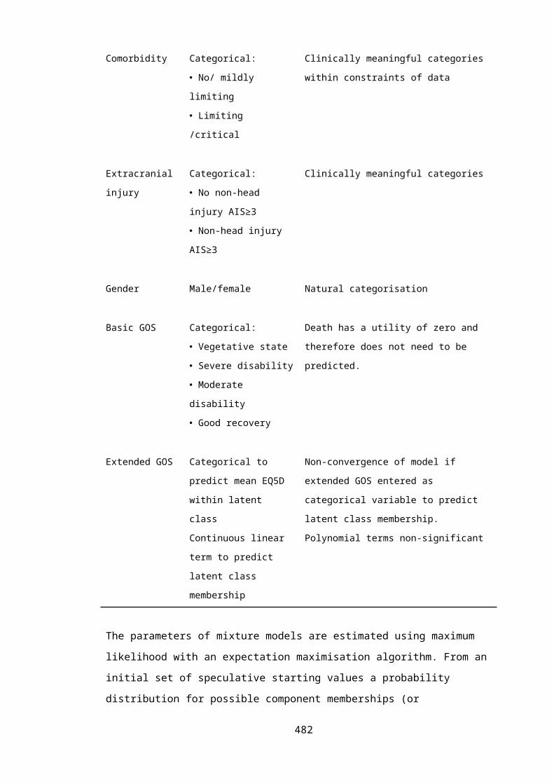
Table G2. Classification of TBI severity

Moderate/severe TBI.Documented head trauma associated with:

Death due to TBI Loss of consciousness ≥30 mins Post traumatic amnesia ≥24 hours Worst Glasgow Coma Scale score <13 in first 24 hours post injury Structural intracranial lesion present:

• Intracerebral hematoma.• Subdural hematoma.• Epidural hematoma.• Cerebral contusion.• Hemorrhagic contusion.• Penetrating TBI (dura penetrated).• Subarachnoid hemorrhage.

Mild TBI.Documented head trauma associated with no moderate/severe criteria, and:

Loss of consciousness <30 mins Post traumatic amnesia <24 hours Worst Glasgow Coma Scale score 13-15 in first 24 hours post injury Structural intracranial lesion present:

• Basilar skull fracture (dura intact)• Linear skull fracture

Post-concussive symptoms:• Blurred vision• Confusion (mental state changes)• Dazed• Dizziness• Focal neurological symptoms• Headache• Nausea

G.1.3 Cohort and period life tables

Life tables conceptually trace a cohort of newborn babies from a defined population through

their entire life; providing a summary of their mortality experience by reporting the probability

of death at each age of life. From this, additional inferences on the number of deaths per year,

expectation of life at a given age, and population survival curves and hazard functions can be

derived. Such information may be of interest in actuarial science, health economics,

epidemiology or biological disciplines.[9-11]

The basic structure of a life table is shown in Table G3. Each row refers to a specific time

period, usually a single year of life. Conventionally there are 7 columns, which are defined as

follows:

482

Age (x): The age at the beginning of a one year interval of life between age x and x+1.

Proportion dying (nqx): The proportion of the cohort dying during each age interval.

This is synonymous with the risk of death during the interval x to x+1, conditional on

surviving to age x.

Number alive (lx): The number of cases alive at the beginning of the age interval. The

initial size of the conceptual cohort is termed the radix and is conventionally set to

100,000. As time progresses the number of living persons declines as individuals die

during each age interval.

Number of deaths (ndx): The number of individuals from the hypothetical cohort dying

during each age interval.

Number of years lived (nLx): The number of years lived by remaining individuals in the

cohort during each age interval. Individuals dying during an age period contribute a

portion of a year to this calculation.

Total time lived (Tx): The total number of years lived by members of the cohort beyond

a given age x.

ex: Expectation of life at age x: The average life expectancy having reached age x.

The subscript before each parameter defines the width of the age interval, usually 1 year. The

subscript after the parameter defines the starting point of the interval i.e. age x. lx, Tx, and ex to

not have an initial subscript as they refer to an exact age x, rather than an age interval. The

conditional probability of dying, nqx, is the basic function of the life table and other values can

be derived from this and the radix.[9-11]

Table G3. The structure of a typical life table.

Age (x) qx lx dx Lx Tx ex

0 0.005683 100,000 568 99,602 2,439,752 76.52

1 0.000406 99,432 40 99,412 2,340,150 75.95

2 0.000249 99,391 25 99,379 2,240,738 74.98

3 0.000207 99,367 21 99,356 2,141,360 74.00

. . . . . . .

. . . . . . .

100 0.389974 613 239 493 493 0.80

Data from published UK general population male life table 2003-2005.[12]

483

Life tables can be constructed for the general public or for more narrowly defined study

populations; and can be based on the average individual or calculated conditional on certain

characteristics such as gender or ethnicity. Further generalisations include multiple-cause life

tables which attribute death to specific causes, or examination of how other outcomes change

with age, such as disability or marital status. Life tables are categorised according to the

intervals over which changes in mortality are observed. Complete life tables display survival

probabilities for each year of life, while abridged life tables examine larger time periods,

commonly every 5 years. Further classification is based on the methodology used for

constructing life tables, designated a cohort or period approach. [9, 10]

Cohort life tables examine the survivorship of a specific birth cohort followed longitudinally

over time. Although they can be produced directly from population experience data, the

difficulties of collecting data of consistently high quality over time mean that cohort tables are

generally based on mortality rates derived from a consecutive series of age-specific mortality

rates. To compile a complete cohort life table the observation period must be sufficiently long

to include all deaths in the incipient population. In contemporary birth cohorts the full

mortality experience will not have been observed and projection of mortality rates, based on

past trends and distributional assumptions, must be made. Recent cohort life tables therefore

involve an element of subjectivity.[9, 10]

In contrast period life tables (also known as current or static life tables) are formulated from

the cross-sectional age-specific mortality rates of the entire population. The probability of

death in the current year is consequently calculated for each age. This has the major

advantage that short term data can used to immediately construct the life table. However, the

derived period life table represents a hypothetical (or synthetic) population to which it is

unrealistically assumed that age-specific mortality rates will continue into the future,

throughout the life of the cohort.[9, 10]

If the population is in equilibrium, and there are no secular trends or period effects affecting

survival, then period and cohort life tables will be equivalent. In reality, cohort tables show a

less rapid increase in death rate with advancing age because the general improvements in

health conditions that occur over time are reflected in succeeding ages. Conversely, period

tables will show a more rapid increase in death rates with age because calendar year

experience for each higher age does not reflect the improved mortality of the succeeding

years. Furthermore, survivor functions from period life tables are more vulnerable to period

effects which may affect the entire population for a brief period e.g. an influenza epidemic or

484

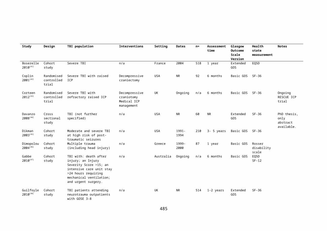
world war, but will only effect the mortality experience of a birth cohort for a short time.

Therefore although period life tables are useful for describing changes in mortality through

time or measuring mortality experienced in a given period, cohort methodology is considered

superior for investigating generational trends in mortality and extrapolating life expectancy. [9,

10]

G.1.4 Sensitivity analyses for informative censoring

Parametric survival analysis assumes that censoring is non-informative.[1] This entails that the

distribution of follow up times for censored cases with the event of interest unobserved,

provides no information on the distribution of survival times observed in patients experiencing

the event, and vice versa. In the REP TBI cohort patients are right censored as a result of

moving away from Olmsted County prior to 2013 (‘lost to follow up’), or remaining alive at the

end of the study period (‘administrative censoring’).

To explore the potential impact of informative censoring, patients who were non-

administratively censored (i.e. prematurely lost to follow up before the end of the study

period) were compared with remaining cases. Chi squared tests were used for categorical

variables. Mann-Whitney U tests were used for non-normally distributed continuous variables.

Extreme case and scenario sensitivity analyses were then conducted, simulating a range of

censoring mechanisms for patients lost to follow up. In worst and best case analyses survival

times were alternatively set to immediate death, or survival until the study end and results

recalculated. These results provide a stringent boundary for the possible effects of informative

censoring. More credible assumptions were tested in two further scenarios:

Twice as many patients who were prematurely lost to follow up died compared with

those remaining under observation. Life expectancy for those lost to follow up and

assumed to have died was 25% less than that of the general US population estimated

from year 2000 cohort life tables.

Three times as many patients who were prematurely lost to follow up died compared

with those remaining under observation. Life expectancy for those lost to follow up

and assumed to have died was 50% less than that of the general US population

estimated from year 2000 cohort life tables.

Model development, analysis and appraisal were identical to the primary models for each

sensitivity analysis.485

G.2 SUPPLEMENTARY RESULTS

G.2.1 Empirical survival curves

Survival curves categorised by gender, presence of extracranial injury, severity of TBI and

ethnicity, are presented in Figures G1 to G4. Crude empirical survivor functions for gender,

presence of extracranial injury and ethnicity were not significantly different (log rank tests,

p=0.34-0.43); whereas a significant difference was apparent between patients with mild and

moderate/severe TBI (log rank test p<0.01). After adjustment for age at TBI there was some

evidence of increased mortality rates associated with male gender (stratified log rank test,

p=0.08), but the effect of TBI severity became non-significant (stratified log rank test, p=0.42).

0.00

0.25

0.50

0.75

1.00

Prop

ortio

n dy

ing

386 316(13) 277(16) 216(13) 100(12) 24(2) 0(0)Males383 316(22) 274(16) 208(12) 99(9) 18(5) 0(0)Females

At-risk tableGender:

0 5 10 15 20 25 30Years after first TBI

Females Males

Figure G1. Survival curve for long term mortality following TBI stratified by gender

486

0.00

0.25

0.50

0.75

1.00

Prop

ortio

n dy

ing

179 149(9) 128(5) 105(4) 49(3) 10(3) 0(0)Extracranial injury590 483(26) 423(27) 319(21) 150(18) 32(4) 0(0)Isolated TBI

At-risk tableType of injury:


Isolated TBI Extracranial injury

Figure G2. Survival curve for long term mortality following TBI stratified by the presence of

extracranial injury

0.00

0.25

0.50

0.75

1.00

Prop

ortio

n dy

ing

210 149(11) 128(6) 94(3) 36(9) 4(2) 0(0)Non-white559 483(24) 423(26) 330(22) 163(12) 38(5) 0(0)White

At-risk tableEthnicity:


White Non-white

Figure G3. Survival curve for long term mortality following TBI stratified by ethnicity

487

Figure G4. Survival curve for six month survivors of TBI stratified by TBI severity

G.2.2 Primary Gompertz model diagnostics

The final Gompertz model was checked for misspecification, goodness of fit, outliers,

influential points and proportionality of hazards:[1]

A link test indicated that the coefficient on the squared linear predictor was non-

significant suggesting no misspecification of the dependent variable (p=0.442).

Log-cumulative hazard plots for different age groups (young adult, middle aged and

elderly) were broadly parallel indicating a proportional hazard assumption was

tenable (Chapter 7).

A smoothed plot (using running means) of age at TBI against Martingale residuals was

approximately linear as shown in Figure G5. This suggests that the first degree

fractional polynomial used for age at TBI in the model is of the correct functional form.

Examination of Cox-Snell residuals revealed some evidence for lack of model fit, with

cumulative hazard deviating from the expected 45 degree line when plotted against

the residuals (Figure G6). However, cumulative hazard demonstrated a linear increase

which departed from the reference line by less than 5º indicating model goodness of

fit was acceptable overall. The divergence in the right hand tail is expected because of

the reduced effective sample caused by prior failures and non-administrative

censoring.

Six observations were identified as potentially influential outliers based on a plot of

Cox-Snell residuals against survival time (Figure G7). All of these cases were elderly

488

patients (84 -92 years) who survived longer than expected. Excluding these

observations improved model fit (AIC 510 v 529 and better fit of Cox-Snell residuals to

cumulative hazard). Extrapolated survival results were not materially changed, with

minimally increased mortality projected in the elderly TBI subgroup, and very similar

mortality rates predicted for middle aged and younger cases. However as these

influential cases were not obviously anomalous it was decided to retain them in

estimation of the final model.

The model comparing survival between TBI cases and non-TBI REP controls was similarly

checked with unremarkable diagnostics.

-3-2

-10

1M

artin

gale

resid

uals

20 40 60 80 100Age at TBI (years)

bandwidth = .8

Figure G5. Functional form of age at TBI assessed plotting Martingale residuals against age at

TBI.

01

23

45

Nelso

n-Aa

len

cum

ulati

ve h

azar

d

0 1 2 3 4Cox-Snell residuals

Nelson-Aalen cumulative hazard Cox-Snell residual

Figure G6. Model goodness of fit assessed by plotting Cox-Snell residuals against Nelson-

Aalen cumulative hazard.489

1

23

4

6

710

11

1215

1619

2021 22

2324

25

2628 29

30

31

32

33

34

35

36

37

3839

42

43

44

4546

474850 525354

55

56 57585961

636465

66

6769

70

72

73

74 75

76

77

7879

80

81

82

83

84

85

86

88

89 90 9192

9394 9596979899100101102

103 105

107

108109110

111112

113

114

115116

117

118119

120121

123124125 126127128

129

130131 132133

134

135 136137 138139

141

142143144

145 146 147148149 150 151152153 154 155156

157158159 160161 162163

164

165 166167 168

169

170171 172173 174175 176177 178179180

181

182183 184 185 186

187

188189190 191192 193194195

196197 198199 200201202203204205206207 208209 210211

212

213 214215216

217218219220221

223224 226 227228

229 230 231232 233234235237238239 241 242

243

244245246 247248249250251252 254257

258259260 261 263 264265 266267 269273 274275276 277278279

280281282283 285286 288 289291 292293 295296 297299300301302 303304305 307308

310 313314316317 320321322 323324 325326 327 333337 339340 341342343

344347348349 351352353 355358 359362 363

365366367 368370 371372 373

374 375376377379 380381382 383384 385386388 389390

391

392 393396399 400 401402 404405406408410 419422 423424 426 430434438 442443 444445 446448454 455457458459 460464466472

473474475478481 485489490

492497

498

499500 502504 506507512 515 516 517519 520522 524527533534538

539540541542544 546551

552

554 556557561 563564565566 568569

570574 575577580581 582584587 591595

596

597600 604607 610615 617618 619622 624628629632 639640641642643 644645 646648650 653 654655 656658661

664 665669671673 677679 681682 683684 689 692 694697698699700701 703707709 710711 715717720722 723724 726733735 736739742 743745 746747750752 753754 756757758759 760 761763764765 767768769771 772773774775776 777778

780

781

782

783

784

785

786

787

788

789

790

793

794795796 797

798

799

801

802

803

804

805

806

807

808810811

812

813

815816

817 818 819

821

822823824

825

826827828

829830

831832

833

834

835

836837838839840841842

843

844

845

846

847

848849850

851 852853

854 855 856 859863 866867868869872 874875876 877878 879883 884886887888 889892 893894 897 898899901 902904907 908 910

911

912915916 917925 927 935 942948 953960 961964 966967 968969

976

981985 988997 10051009 101410161028

1031 1033 10341035 103910401044 104510471052 105410551056 10581060 10621072 1074

1075

10761077 107810811082 10831084 1087

1088

1093 10951099 11061107111311141115

1117

1118 112011211122 11251127 113011321135 11381139 1143 114411451146

11471150 1153 115611571158

1159

1160 11621163 1164

1165

1167 116811701172 11731176 1178 1179 1180

1182

1183 118411851186 1187

119011911192

119411951196

1198120512061207 120812091210 121112121213 121412151217 12191220

12211222 12241226 1227 1228 12291230 1232

1233

1234 12351236 1239

1240

12411242 12431244 1246

1247

1248

1250

1255 1256

1257

01

23

4Co

x-sn

ell r

esid

uals

0 10 20 30Suvival time

Figure G7. Cox-snell residuals for individual cases plotted against survival time

G.2.3 Primary model appraisal: Comparison of predicted life expectancy

Predicted median survival from the Gompertz model following a TBI at the ages of 25, 52 and

79 years were 45.8 years (95%CI 38.0-53.6), 30.6 years (95%CI 26.8-34.5) and 9.0 years (95%CI

7.8-10.3) respectively. These predictions were consistent with previously published estimates

for TBI life expectancy as shown in Table G4.

490

Table G4. Comparison of predicted life expectancy results from REP Gompertz model with

other published estimates.

Study Population Recruitment period

Survival time (years)

Current study Adults>16yearsUSAny TBISurviving ≥6 months

1987-1999 TBI aged:Median survival:

25y46

52y31

79y9

Ventura 2010[13]

Any ageUSTBI discharged alive after acute hospitalisation

1998-2003 TBI aged:Mean survival:

20y47

50y22

80y5

Felix-Harrison 2009[14]

Adults >16yearsUSTBI admitted for rehabilitationSurviving 1 year


20y50

50y23

70y9


Adults >16yearsUSTBI admitted for rehabilitation


20y54

50y20

70y7

Strauss 1998[16]

Aged 5-21 yearsUSTBI receiving disability services


20y51

50y27

--

G.2.4 Primary model appraisal: External validity of Weibull model

Table G5. Comparison of metrics for assessing the goodness of fit to REP data for Gompertz

and Weibull parametric survival models.

Distribution Predicted survival function v period general population life tables

Median predicted survival time (years) with age at TBI of*:

25y 52y 79yGompertz Very similar pattern for all age groups 46 31 9

Weibull Similar pattern for elderlyVery dissimilar pattern for other age

groups

116 45 9

*estimates unadjusted for cohort effects.

491

25 years

52 years

79 years

0.2

.4.6

.81

Prop

ortio

n dy

ing

0 10 20 30 40 50 60 70 80Years after first TBI

Figure G8. Comparison of predicted extrapolative estimates of survival following TBI sustained at

certain ages using a Weibull distribution compared with the year 2000 US general population cohort

life tables. Black lines present the survival curves estimated from the Weibull model following TBI

sustained at illustrative ages. Grey lines indicate the corresponding US general population survival

curves for patients of the same age based on cohort life table data.

G.2.5 Secondary models: Effect of age at TBI and gender on survival

Model development

Based on theoretical considerations,[17] and the suggestion of a sex effect on mortality rates

from exploratory analyses of the empirical survivor function, a secondary model was

developed including gender. Exploratory analyses and previous studies suggested no influence

of TBI severity on post-acute survival. Presence of extracranial injury was not significantly

associated with survival time in univariate analysis and did not add predictive power. Given

that economic models tend to focus on average populations, and these initial analyses did not

suggest an effect on survival from ethnicity or the presence of extracranial injury, more

detailed models were not developed.

Weibull and Gompertz proportional hazard models were again identified as potentially suitable

based on graphical plots: linear log cumulative hazard (log-log survival) plots stratified by

gender and adjusted for age at TBI using the Cox model for the Weibull distribution (Figure

G9); and smoothed log-hazard plots for age-groups categorised by gender for the Gompertz

distribution (Figure G10).

492

-8-6

-4-2

Log

cum

ulati

ve h

azar

d

-1 0 1 2 3Log time after TBI (years)

Females MalesGender (adjusted for age at TBI):

Figure G9. Log cumulative hazard plotted against time for a Cox model stratified by gender

and adjusted for age at first TBI,

-6-4

-20

Log

haza

rd

0 5 10 15 20Time after TBI (years)

Young females Young malesMiddle aged females Middle aged malesElderly females Elderly males

Group:

Figure G10. Log hazard plotted against survival time after TBI stratified by gender and age

group.

493

Non-linearity of the effect of age at TBI was accounted for by evaluating the best fitting

fractional polynomial. Gender was included as a binary variable. There was no evidence of

change in distribution shape with increasing age or change in gender, and no unexplained

heterogeneity or time-varying age coefficients.

The Gompertz model demonstrated a better fit to the REP data compared with a Weibull

distribution with lower information criterion statistics (AIC 526.0 v 528.7, BIC 544.6 v 547.3).

Survival curves from this model demonstrated satisfactory fit to the observed Kaplan-Meier

curves for each age group and gender, with virtually all predicted survival probabilities

(calculated for the median age of each age category) remaining within the 95% confidence

interval bounds as demonstrated in Figure G11. All model diagnostics were unremarkable, with

no evidence for any model misspecification.

494

16-39 age group

40-64 age group

>65 age group

0.2

.4.6

.81

Prop

ortio

n su

rviv

ing

0 10 20 30Years after first TBI (males)

16-39 age group

40-64 age group

>65 age group

0.2

.4.6

.81

Prop

ortio

n su

rviv

ing

0 10 20 30Years after first TBI (females)

Figure G11. Gompertz model predicted survival probabilities for males and females compared with

the observed Kaplan-Meier curves over the study period for secondary model including age at TBI and

gender. Lines represent the Kaplan-Meier derived survival function for young, middle aged and elderly

age groups. 95% confidence intervals for this empirical survivor function are shaded in grey. Symbols

present the predicted survivor function from the Gompertz model for the median age of patients within

each age group (25, 52 and 79 years respectively). Top panel= males. Bottom panel=females.

495

The Gompertz model appeared to provide plausible long term survival estimates when

compared with gender specific Minnesota general population decennial period life tables from

the same era as the study cohort. Illustrative extrapolated survival functions for TBI patients at

25, 52 and 79 years of age were indistinguishable in pattern from the corresponding year 2000

general population survival curves, as shown in Figure G12. Predicted median survival

following a TBI at the ages of 25, 52 and 79 years for males were 44.2 years (95%CI 36.8-51.6),

29.9 years (95%CI 25.2-32.7) and 7.7 years (95%CI 6.0-9.4) respectively. The corresponding

median survival times for females sustaining TBI at the same ages were: 48.5 (95%CI 39.6-

57.4), 33.2 (95%CI 28.3-38.1) and 10.4 (95% CI 8.8-12.0) years. An identical pattern, but

demonstrating the expected lower relative survival for patients following TBI, was also

observed when comparing extrapolated TBI survival curves with those from gender-specific US

general population cohort life tables from the year 2000 (Figure G13). The final model

coefficients and covariance matrix are summarised in Table G6.

Table G6. Coefficients and covariance matrix for final Gompertz model for extrapolation of

survival following TBI, accounting for age at first TBI.

Model Coefficients (se)

β0 β1 β2 γh(t|age)=e(β0+β1x1+β2x2).eγt -7.07(0.33)

0.077(0.004)

0.455(0.19)

0.103(0.18)

Where:

x1=(age at TBI/10)2 -13.54

x2=0 if female, x2=1 if male

t=years after TBI

Variance-covariance matrix

β0 β1 β2 γ

β0 0.11

β1 -0.0012 0.00002

β2 -0.025 0.0002 0.036

γ -0.0046 0.000045 0.000065 0.0003

496

25 years

52 years

79 years

0.2

.4.6

.81

Prop

ortio

n dy

ing

0 10 20 30 40 50 60 70 80Years after first TBI (males)

25 years

52 years

79 years

0.2

.4.6

.81

Prop

ortio

n dy

ing

0 10 20 30 40 50 60 70 80Years after first TBI (females)

Figure G12. Comparison of predicted extrapolative estimates of survival for males and females

following TBI sustained at certain ages compared with the year 2000 Minnesota general population

period life tables.1 Black lines present the survival curves estimated from the Gompertz model following

TBI sustained at illustrative ages. Grey lines indicate the corresponding Minnesota population survival

curves (based on cross sectional mortality rates) for patients of the same age. Top panel= males. Bottom

panel=females.

1 Period life tables use current age-specific mortality experience to project future life expectancy and will underestimate the true survivor. This will give the spurious appearance that survival following TBI at older ages is similar to the Minnesota general population.

497

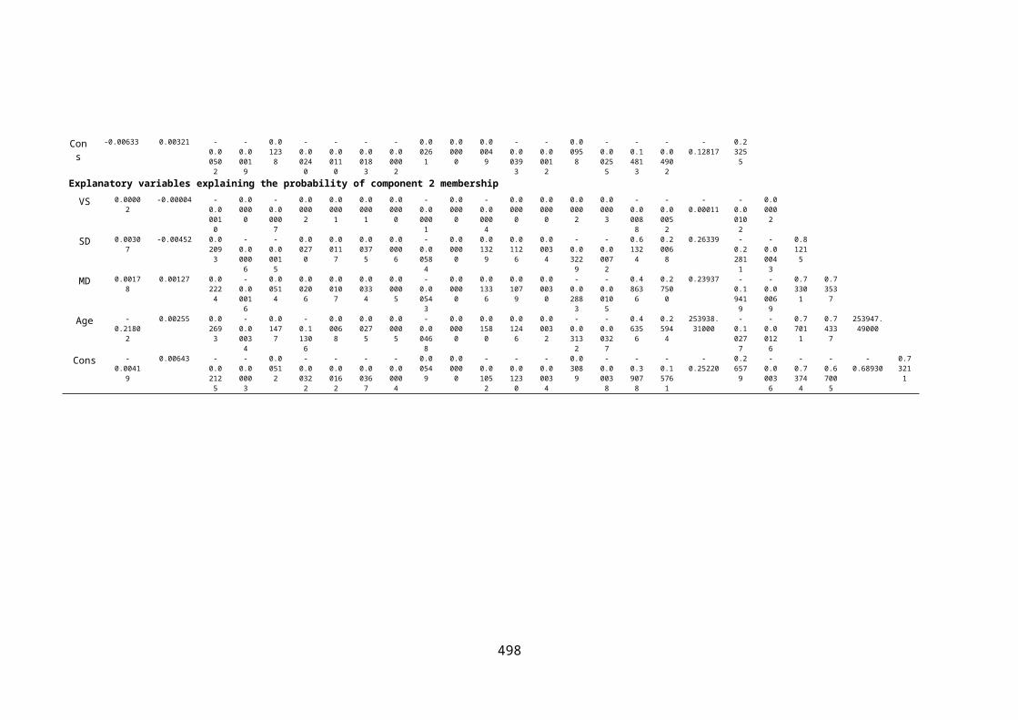
Figure G13. Comparison of predicted extrapolative estimates of survival for males and females

following TBI sustained at certain ages using a Gompertz distribution compared with gender specific

year 2000 US general population cohort life table. Black lines present the survival curves estimated

from the Gompertz model following TBI sustained at illustrative ages. Grey lines indicate the

corresponding US general population survival curves for patients of the same age based on gender

specific cohort life table data.

498

G.2.6 Secular trends in US Cohort life tables

Table G7. Change in shape and scale parameter of Gompertz hazard functions optimally

fitting US cohort life table data between 1900 and 2010.

Shape Scale Log-scale Shape %

change*

Log scale %

change*

2010 0.09525

6

0.0000192

1

-10.86007958 1.003375 1.007421

2000 0.09493

6

0.0000208

1

-10.78007692 1 1

1990 0.09459

7

0.0000226

3

-10.6962341 0.996426 0.992222

1980 0.09423

2

0.0000247

3

-10.60749348 0.992584 0.983991

1970 0.09384

2

0.0000271

6

-10.51376526 0.98848 0.975296

1960 0.09341

6

0.0000300

1

-10.4139799 0.98399 0.966039

1950 0.09294

3

0.0000334

2

-10.30635603 0.979008 0.956056

1940 0.09241

8

0.0000375 -10.19116962 0.973473 0.945371

1930 0.09203

4

0.0000415

6

-10.08837239 0.969431 0.935835

1920 0.09266

8

0.0000416 -10.08741039 0.976109 0.935746

1910 0.09421 0.0000366

3

-10.21464298 0.99235 0.947548

1900 0.08571

1

0.0000756

2

-9.48978976 0.902827 0.880308

*year 2000 used as baseline year for calculation of proportional change

499

.97

.98

.99

11.

01%

cha

nge

in G

ompe

rtz

dist

ributi

on sh

ape

-80 -60 -40 -20 0 20

Years from 2000

Figure G14. Observed changes in Gompertz distribution shape parameter fitted to US life

table data over time, compared with fitted values from non-linear regression model.

Circles represent observed changes in shape parameter compared with year 2000 baseline. Line

represents predicted values from fitted quadratic function.

.94

.96

.98

11.

02%

cha

nge

in lo

g-sc

ale

para

met

er

-80 -60 -40 -20 0 20

Years from 2000

Figure G15. Observed changes in Gompertz distribution log-scale parameter fitted to US life

table data over time, compared with fitted values from non-linear regression model.

Circles represent observed changes in shape parameter compared with year 2000 baseline. Line

represents predicted values from fitted quadratic function.

500

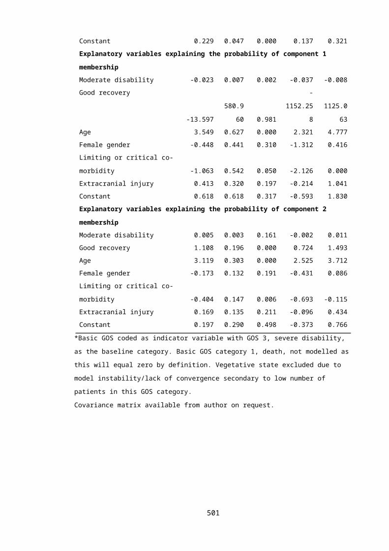
Table G8. Quadratic models fitted to proportional change in shape and scale of Gompertz

distributions over consecutive generational hazard functions

Model* Coefficients (se) RMSE Adj R2

Squared

term

Linear

term

Intercep

t

Shape y=-1E-06x2 + 0.0004x + 1.0

-1.32e-06(2.1e-7)

0.0004(0.00001)

1.00 (0.0002)

0.0004

0.999

Log-scale y=-2E-06x2 + 0.0008x +

1.0

-2.31e-06(1.95e-07)

0.0008(0.00001)

1.00(0.0002)

0.0003

0.9998

*Where y is proportional change in Gompertz distribution shape/log-scale parameter; and x is each year

after the year 2000.

G.2.7 Formulas for Gompertz survival, cumulative hazard and probability density functions

Table G9. Functions of Gompertz distribution

Function Explanation Formula

Probability

density function

Probability of death at a given age f(t|age)= 𝜆eγt. exp{λ/γ(1-eγt)}Survivor

function

Proportion surviving at time t, conditional on

age at first TBI

S(t|age)=exp{λ/γ(1-eγt)}

Hazard function Hazard of death at time t, conditional on age at

first TBI

h(t|age)=𝜆eγt

Cumulative

hazard function

Cumulative hazard of death at time t,

conditional on age at first TBI

H(t|age)=γ-1 exp(λ){exp(γt)-1}γ = Gompertz distribution shape parameter, λ= Gompertz distribution scale parameter, e=Euler’s number, t=number of years since sustaining TBI.

501

G.2.8 Sensitivity analyses for non-informative censoring.

Characteristics of censored patients

Non-administratively censored patients were predominantly younger (median age 25.8 v 33.8,

p<0.01), non-white (40.9% v 22.4%, p<0.01), sustained more mild TBI (97.0% v 91.9%, p=0.01)

and were victims of relatively more sporting accidents (14.8% v 7.2%, p=0.001). However, after

controlling for age, drops outs were broadly representative of remaining patients with no

notable differences except for a higher proportion of non-white ethnicity in the young adult

subgroup (11% v 4%, p<0.01). The overall characteristics of patients prematurely lost to follow

up are contrasted to administratively censored or dead patients in Table G9. Features of cases

lost to follow up are further compared, stratified by age group, in Table G10.

Table G10. Overall characteristics of patients lost to follow up compared with

administratively censored or dying patients

Patient characteristic(n=769)

Administratively censored or died

(%, 95%CI)

Non-administratively censored

(%, 95%CI)

p-value

n=566 n=203

Age (Years, median, IQR) 33.8 years (22.5-55.0) 25.8 (19.8-31.6) <0.01

Male Gender 49.1% (45.0-53.2) 53.2% (46.3-60.1) 0.32

White ethnicity* 77.6% (74.1-81.0) 59.1% (52.3-65.9) <0.01

Extracranial injury 23.5% (20.0-27.0) 22.7% (16.9-28.4) 0.81

Mild TBI 91.9% (89.6-94.1) 97.0% (94.7-99.4) 0.01

Mode of injury

Road accident 43.4% (39.4-47.6) 44.3% (37.5-51.2)

Fall 27.7% (24.0-31.4) 16.3% (11.1-21.4)

Sports-related 7.2% (5.1-9.4) 14.8% (9.9-19.6)

Bunt assault 7.6% (5.1-9.4) 8.4% (4.5-12.2)

Other 14.0% (11.1-16.8) 16.3% (11.2-21.4) 0.001

502

Table G11. Characteristics of patients lost to follow up compared with administratively censored or dying patients stratified by age group.

Patient characteristic

n= Completeness index (%)

Male gender

Non-white ethnicity

Extracranial injury

Mild TBI Mode of injury: RTA

Mode of injury: Fall

Mode of injury: Assault

Mode of injury: Other

Young adults (16-39 years) 72.5%

Lost to follow up 182 53.3% 11.0% 22.0% 97.3% 44.5% 15.4% 8.8% 31.3%


357 51.8% 4.5% 23.8% 94.4% 51.3% 14.0% 9.0% 33.8%

p-value 0.75 <0.01 0.63 0.14 0.39

Middle aged(40-39 years) 90.7%

Lost to follow up 18 55.6% 5.6% 33.3% 94.4% 50.0% 11.1% 5.6% 33.3%


121 52.9% 2.5% 23.1% 90.1% 39.7% 33.1% 8.3% 18.9%

p-value 0.83 0.45 0.35 0.55 0.23

Eldery(>65 years) 95.5%

Lost to follow up 3 33.3% 0% 0% 100% 0% 100% 0% 0%


88 33.0% 1.1% 22.7% 84.1% 17.1% 76.1% 1.1% 5.7%

p-value 0.99 0.61 0.35 0.45 0.92

503

Sensitivity analyses for non-informative censoring

Extreme case sensitivity analyses applied maximal stress to the robustness of study results. A

Gompertz distribution maintained satisfactory goodness of fit to the data in the event that all

study drop outs immediately died after leaving Olmsted County. However the resulting survival

curves were completely implausible, precluding any insight into the effect of censoring. In the

opposite eventuality that all cases lost to follow up survived to the of the study period

significantly diminished survival was still apparent for TBI patients compared with the general

US population.

In scenario analyses exploring more plausible censoring mechanisms TBI patients

demonstrated notably worse survival compared with base case estimates. In the first scenario

it was assumed that twice as many patients who were prematurely lost to follow up died

compared with those remaining under observation. Life expectancy for those lost to follow up

and assumed to have died was 25% less than that of the general US population estimated from

year 2000 cohort life tables. Predicted median survival following a TBI at the ages of 25, 52 and

79 years were 38.9 years (95%CI 36.7-41.4), 27.9 years (95%CI 26.5-29.2) and 9.15 years

(95%CI 8.1-12.1) respectively; compared with 45.8 (38.0-53.6), 30.6 (26.8-34.5) and 9.0 (7.8-

10.3) in the original primary model.

In the second scenario three times as many patients who were prematurely lost to follow up

were assumed to die compared with those remaining under observation. Life expectancy for

those lost to follow up and assumed to have died was 50% less than that of the general US

population estimated from year 2000 cohort life tables. Under these circumstances predicted

median survival following a TBI at the ages of 25, 52 and 79 years were 34.1 years (95%CI 31.8-

36.4), 25.0 years (95%CI 23.7-26.3) and 9.3 years (95%CI 8.3-10.4) respectively.

Figure G16 presents the extrapolated survival curves from each sensitivity analysis compared

with the year 2000 general population. Table G11 compares predicted median survival times

with those from the primary model. Diagnostics for survival models developed in these

sensitivity analyses were unremarkable.

504

25 years

52 years

79 years

0.2

.4.6

.81

Prop

ortio

n dy

ing

0 10 20 30 40 50 60 70 80

Years after first TBI

25 years

52 years

79 years

0.2

.4.6

.81

Prop

ortio

n dy

ing

0 10 20 30 40 50 60 70 80


25 years

52 years

79 years

0.2

.4.6

.81

Prop

ortio

n dy

ing

0 10 20 30 40 50 60 70 80


25 years

52 years

79 years

0.2

.4.6

.81

Prop

ortio

n dy

ing

0 10 20 30 40 50 60 70 80


Figure G16. Gompertz model predicted extrapolative estimates of survival following TBI in sensitivity analyses for non-informative censoring. Black lines present the survival curves estimated for

survival following TBI sustained at illustrative ages . Grey lines indicate the corresponding survival curves for the US general population, derived from year 2000 cohort life tables. a) Worst case

sensitivity analysis: all patients lost to follow up die immediately. b) Best case: All patients lost to follow up survive until the study end. c) Scenario analysis: Twice as many drops die with life

expectancy 25% that of the general population. d) Scenario analysis: Thrice as many drops die with life expectancy 50% that of the general population.

505

Table G12. Predicted median survival time from sensitivity analyses examining non-

informative censoring.

Model Predicted median survival (years, 95% CI)

25 years 52 years 79 Years

Primary model 45.8(38.0-53.6)

30.6(26.8-34.5)

9.0(7.8-10.3)

Worst case sensitivity analysis 111.0(0.0-1,278.0)

26.2(19.6-32.9)

6.8(5.2-8.5)

Best case sensitivity analysis 49.0(39.9-58.1)

32.9(28.3-37.4)

9.6(8.3-10.9)

First scenario sensitivity analysis* 38.9(36.7-41.1)

27.9(26.5-29.2)

9.15(8.1-10.1)

Second scenario sensitivity analysis** 34.1(31.8-36.4)

25.0(23.7-26.3)

9.34(8.3-10.4)

* Twice as many patients who were prematurely lost to follow up died compared with those remaining under observation. Life

expectancy for those lost to follow up and assumed to have died was 25% less than that of the general US population.

* Thrice as many patients who were prematurely lost to follow up died compared with those remaining under observation. Life

expectancy for those lost to follow up and assumed to have died was 50% less than that of the general US population.

506

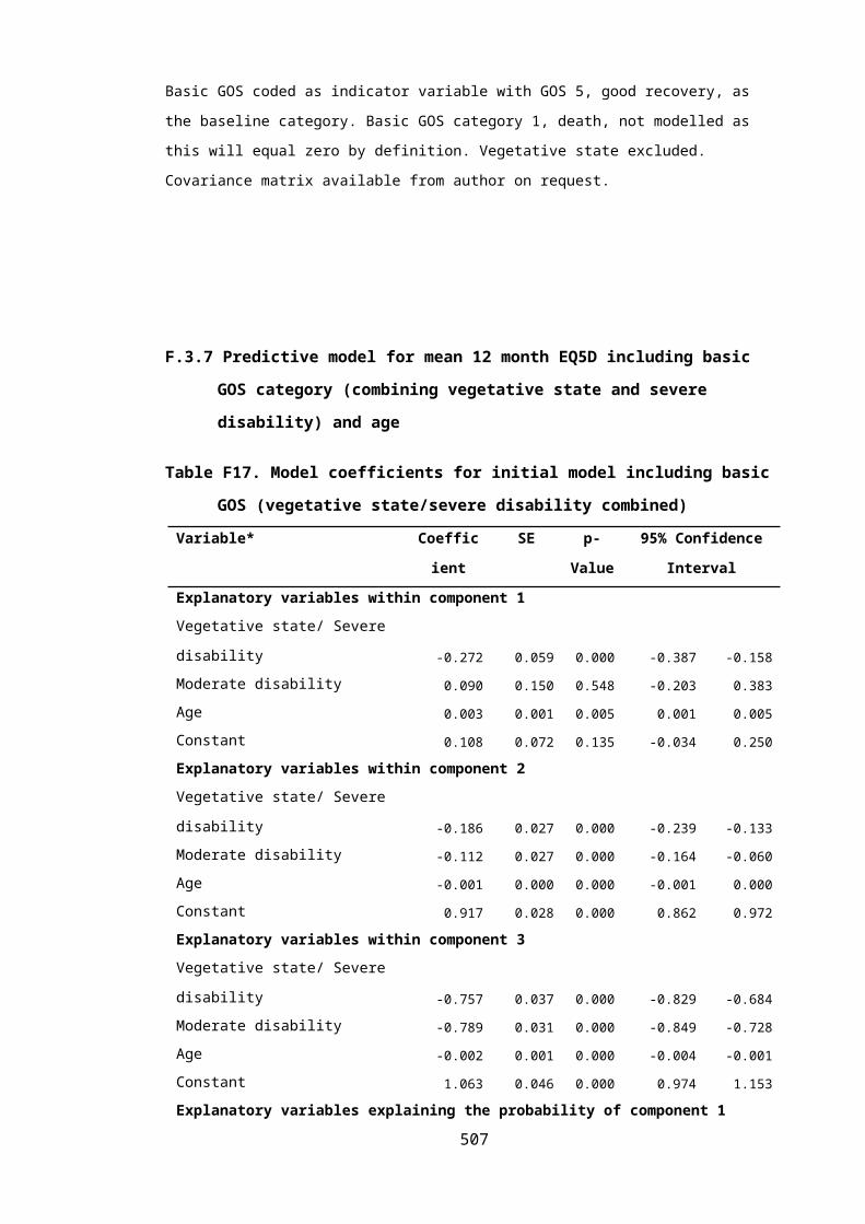
G.2.9 Comparison of REP model survival predictions to survival function derived from 2012

UK period life tables

Figure G17. Comparison of REP model survival predictions to survival function derived from

2012 UK period life tables.

Survival curve shown for 50 year old patient in 2012. Grey triangles represent survival function from REP

model adjusted for cohort effects. Shaded area indicated 95% confidence interval for REP survival

estimates. Black line presents survival function form UK general population period life table.

507

G.2.10 Summary of findings from previous studies examining long term survival after TBI

Table G13. Studies investigating long term mortality following TBI

Study* Design Recruitment period

End of follow up

Setting Study population n= Methodology Observed effect of TBI on survival

Effect estimate(95% CI)

% deaths during study period

Mean age(sd)

% Male(95%

CI)

Current study

RCS 1987-1999 2013 Minnesota, US Adults >16 yrsPost-acute mild –severe TBI

769 Parametric survival analysis

Decreased compared with general population

HR: 1.47 (1.15-1.86)

Life expectancy at§:25=46 years52=31 years79=9 years

24% 30.3 (19.8)

50% (47-54)

Fazel 2014[18]

RCS 1969-2009 2009 Sweden Any hospital admission or outpatient attendance for TBI

218,300 Conditional Logistic regression using age/gender matched community controls; or sibling controls


OR: 3.2 (3.0-3.4) [general population]

OR: 2.6 (2.3-2.8) [siblings]

22% 18.6 69%

Baguley 2012[19]

RCS 1990-2007 2009 New South Wales, Australia

Adults >16 yrsTBI admitted for rehabilitation

2,545 SMR calculated using national general population mortality rates


SMR: 3.19 (2.8 –3.6) 10.2% 35 (14)

81%

Himanen 2011[20]

RCS 1950-1971 1996 Turku, Finland Adults >16 yrsTBI referred for neurological clinic assessment

192 SMR calculated using national general population mortality rates


SMR: 1.25 (0.99–1.57) 39% 37.0 (13.8)

65%

Ventura RCS 1998-2003 2005 Colorado, US TBI discharged 18,998 SMR calculated Decreased SMR: 2.47 (2.3 –2.7) 13.1% 40 65%

508

2010[13] alive after acute hospitalisation

using national general population mortality rates

Life expectancy based on SMR & general population mortality rates†

compared with general population

Life expectancy at:20=47 years50=22 years80=5 years

McMillan 2010[21]

RCS 1995-1996 2009 Glasgow, UK TBI with acute hospitalisation

757 Odds of death during follow up compared with age/gender matched non-TBI community controls

Comparison of mortality rates with age/gender matched non-TBI controls

Decreased compared with non-head injured controls

OR 9.4 (95%CI 5.35-16.5)

31 v 14 deaths/100,000/year

33.6%‡ NR NR


RCS 1961-2002 2003 Colorado, USA Adults >16yearsTBI admitted for rehabilitation & surviving 1 year


Life expectancy based on SMR & general population mortality rates†


SMR: 1.51 (1.25 –1.78)

Life expectancy at:20=50 years50=23 years70=9 yearsfor white males

7.7% 32 76%

509

Colantonio 2008[22]

RCS 1993-1995 2002 Ontario, Canada

Adults >15yearsTBI admitted with ISS>12


SMR calculated using Poisson regression and lower limb injury controls adjusted for age, co-morbidities,


Decreased compared with injury controls

SMR: 2.9

RR 1.67 (1.15-2.40)

NR NR 71%

Cameron 2008[23]

RCS 1988-1991 10 years following injury

Manitoba, Canada

Adults 16-64TBI with acute hospitalisationExcluding first 60 days post injury

1,290 Rate ratio for mortality between TBI & non-injured controls (matched on age, gender, location)

Decreased compared with non-injured ocntrols

RR: 3.35 (2.45–4.59) (controlling for age, gender, location)

RR:1.48 (1.02-2.15)(controlling for age, gender, location, comorbidities & excluding death within 60 days)

12.6% 33.6 69%

Ratcliff 2005[24]

RCS 1974-1984, 1988, 1989

24 years post injury

Pittsburgh, USA

Adults 16-64Moderate & severe TBI discharged from inpatient rehabilitation

642 SMR calculated using regional general population mortality rates

Decreased compared with regional population

SMR: 2.78 19.7% 34.8 73%


RCS 1988-2000 2001 US rehabilitation hospitals

Adults >16yearsTBI admitted for rehabilitation


Life expectancy


SMR: 2.00 (1.69-2.31)

Life expectancy at:

7.4% 37.3 76%

510

based on SMR & general population mortality rates†

20=54 years50=20 years70=7 yearsfor white males

Shavelle 2001[25]

RCS 1988-1996 1997 California, US TBI with mental disability requiring long term careAged >10 yearsSurvived >12 months

2,320 SMR calculated using regional general population mortality rates


SMR: 3.1 (2.5, 3.7) 5.1% NR 68%

Strauss 1998[26]

RCS 1987-1995 1995 California, US TBI receiving disability servicesAged 5-21 years

946 Period life table constructed for TBI patients


TBI at 17 years with resultant moderate motor skills: 89% survival at age 50

Life expectancy at:20=51 years50=27 yearsfor TBI with good mobility

4% NR NR

* Final study included if multiple reports on same cohort. † assuming constant SMR at all ages. ‡ excluding cases who died in first year. § Unadjusted for cohort effectsNR: Not reported

511

G.3 REFERENCES

1. Collett D: Modelling survival data in medical research, 2nd ed. edn. Boca Raton, Fla. ; London: Chapman & Hall/CRC; 2003.

2. Ishak KJ, Kreif N, Benedict A, Muszbek N: Overview of parametric survival analysis for health-economic applications. PharmacoEconomics 2013, 31(8):663-675.

3. Grieve R, Hawkins N, Pennington M: Extrapolation of survival data in cost-effectiveness analyses: improving the current state of play. Medical decision making : an international journal of the Society for Medical Decision Making 2013, 33(6):740-742.

4. Latimer NR: Response to “Survival Analysis and Extrapolation Modeling of Time-to-Event Clinical Trial Data for Economic Evaluation: An Alternative Approach” by Bagust and Beale. Medical Decision Making 2013.

5. Cortese G, Scheike TH, Martinussen T: Flexible survival regression modelling. Statistical methods in medical research 2010, 19(1):5-28.

6. Latimer NR: Survival analysis for economic evaluations alongside clinical trials--extrapolation with patient-level data: inconsistencies, limitations, and a practical guide. Medical decision making : an international journal of the Society for Medical Decision Making 2013, 33(6):743-754.

7. Durrleman S, Simon R: Flexible regression models with cubic splines. Statistics in medicine 1989, 8(5):551-561.

8. Malec JF, Brown AW, Leibson CL, Flaada JT, Mandrekar JN, Diehl NN, Perkins PK: The mayo classification system for traumatic brain injury severity. J Neurotrauma 2007, 24(9):1417-1424.

9. Wunsch GJ, Mouchart M, Duchene J: The life table : modelling survival and death. Dordrecht ; Boston: Kluwer Academic; 2002.

10. Chiang CL: The life table and its applications, Original edn. Malabar, Fla.: R.E. Krieger Pub. Co.; 1984.

11. Gray AM: Applied methods of cost-effectiveness analysis in health care. Oxford: Oxford University Press; 2011.

12. Statistics OoN: England, Interim Life Tables 1980-82 to 2006-2008. In. London: Office of National Statistics; 2009.

13. Ventura T, Harrison-Felix C, Carlson N, Diguiseppi C, Gabella B, Brown A, Devivo M, Whiteneck G: Mortality after discharge from acute care hospitalization with traumatic brain injury: a population-based study. Archives of physical medicine and rehabilitation 2010, 91(1):20-29.

14. Harrison-Felix CL, Whiteneck GG, Jha A, DeVivo MJ, Hammond FM, Hart DM: Mortality over four decades after traumatic brain injury rehabilitation: a retrospective cohort study. Archives of physical medicine and rehabilitation 2009, 90(9):1506-1513.

15. Harrison-Felix C, Whiteneck G, DeVivo M, Hammond FM, Jha A: Mortality following rehabilitation in the Traumatic Brain Injury Model Systems of Care. NeuroRehabilitation 2004, 19(1):45-54.

16. Strauss D, Shavelle RM, DeVivo MJ, Harrison-Felix C, Whiteneck GG: Life expectancy after traumatic brain injury. NeuroRehabilitation 2004, 19(3):257-258.

17. Johansson S: Longevity in women. Cardiovascular clinics 1989, 19(3):3-16.18. Fazel S, Wolf A, Pillas D, Lichtenstein P, Langstrom N: Suicide, fatal injuries, and other

causes of premature mortality in patients with traumatic brain injury: a 41-year Swedish population study. JAMA psychiatry 2014, 71(3):326-333.

19. Baguley IJ, Nott MT, Howle AA, Simpson GK, Browne S, King AC, Cotter RE, Hodgkinson A: Late mortality after severe traumatic brain injury in New South Wales: a multicentre study. The Medical journal of Australia 2012, 196(1):40-45.

512

20. Himanen L, Portin R, Hamalainen P, Hurme S, Hiekkanen H, Tenovuo O: Risk factors for reduced survival after traumatic brain injury: a 30-year follow-up study. Brain injury : [BI] 2011, 25(5):443-452.

21. McMillan TM, Teasdale GM, Weir CJ, Stewart E: Death after head injury: the 13 year outcome of a case control study. Journal of neurology, neurosurgery, and psychiatry 2011, 82(8):931-935.

22. Colantonio A, Escobar MD, Chipman M, McLellan B, Austin PC, Mirabella G, Ratcliff G: Predictors of postacute mortality following traumatic brain injury in a seriously injured population. The Journal of trauma 2008, 64(4):876-882.

23. Cameron CM, Purdie DM, Kliewer EV, McClure RJ: Long-term mortality following trauma: 10 year follow-up in a population-based sample of injured adults. The Journal of trauma 2005, 59(3):639-646.

24. Ratcliff G, Colantonio A, Escobar M, Chase S, Vernich L: Long-term survival following traumatic brain injury. Disability and rehabilitation 2005, 27(6):305-314.

25. Shavelle RM, Strauss D, Whyte J, Day SM, Yu YL: Long-term causes of death after traumatic brain injury. American journal of physical medicine & rehabilitation / Association of Academic Physiatrists 2001, 80(7):510-516; quiz 517-519.

26. Strauss DJ, Shavelle RM, Anderson TW: Long-term survival of children and adolescents after traumatic brain injury. Archives of physical medicine and rehabilitation 1998, 79(9):1095-1100.

513

H APPENDIX H: SUPPLEMENTARY METHODOLOGICAL INFORMATION FOR THE HITSNS

ECONOMIC EVALUATION

H.1 DELPHI SURVEY OF TBI EXPERTS

H.1.1 Background

To optimise the models contextual relevance, reduce biases arising from the subjective views

of expert advisory panel members, maximise content and face validity, and increase credibility

a modified Delphi approach was used to support development of the conceptual models,

seeking a consensus on the economic model structure and included comparators.

The Delphi method is a consensus development technique, extensively applied in health

research and used previously in decision analysis model structuring.[1, 2] The classical Delphi

process consists of a series of consecutive structured surveys of experts’ opinions, interspersed

with moderated feedback to participants, aiming to reach a concordant group response. The

fundamental characteristics of the Delphi technique include: respondent anonymity promoting

the uninhibited expression of opinions; statistical aggregation of group responses; and

controlled feedback and iteration allowing participants to refine their views in light of group

opinions.[2-7]

The initial Delphi iteration traditionally comprises an open survey of panel members’ views to

identify relevant themes with high content validity. Subsequent Delphi rounds then frame and

develop these important items as close-ended statements, with experts rating their agreement

level in view of the group’s overall response, typically scored using a Likert scale. The Delphi

process concludes once sufficient consensus and stability of opinion is reached. This is defined

objectively based on pre-specified proportions of responses falling within in a prescribed

range, and statistical agreement in responses between rounds.[2-7]

A Delphi approach was chosen to support model structuring over other consensus techniques

due to its ability to include a wide range of geographically separated participants, allowance

for reflection and free expression of opinions, efficiency, and facility to distil a diverse range of

opinions.[3]

514

H.1.2 Methods

The classical Delphi approach was modified slightly in response to the study’s objectives with

replacement of an open first round with an advisory panel meeting to define relevant

structured questions and informal judgement used to determine consensus. These

modifications have been implemented previously in health economic studies, reflecting the

specific requirements of decision analysis model structuring.[1, 8]

Purposive sampling was used to recruit a heterogeneous group of subjects encompassing the

full spectrum of expertise relevant to United Kingdom TBI management pathways. Selection

criteria included: subject knowledge; specialist background; likelihood of participation;

advocacy for specific management pathways; and credibility to the decision maker. Experts

were identified from the scientific literature, clinical guideline groups, professional

organisations and personal contacts. The sample size for Delphi studies is subjective and 22

panel members were chosen in accordance with guidelines from the Research And

Development (RAND) Corporation.[2] This number was considered sufficient to reflect the

diversity of potential viewpoints, allow for attrition, and reduce group error.

Potential experts were invited to participate by email and supplied with an information sheet

explaining the study rationale, planned methodology, and consent procedures. An internet

based self-administered Delphi process was subsequently conducted using pre-piloted web-

hosted questionnaires. Each round allowed 2 weeks for completion of responses, with email

reminders sent after 1 week. The survey was conducted from 20th May 2013 to 31st July 2014.

In the first round structured questions, informed by systematic literature reviews and the

advisory group, were posed in three domains: identification of comparators relevant to the

decision problem; characterisation of important population subgroups; and establishment of

factors influencing the effectiveness of possible management pathways. In total 15 questions

were asked across these domains. Participants were asked to rate their agreement with each

question on a 1 (strongly disagree) to 5 (strongly agree) Likert scale and to justify their opinion

in free-text. An additional open question was posed in each domain asking participants to

identify any further important options that had not been included.

A mixed-methods approach was taken to summarise each round’s findings. Quantitative

measures of percentage agreement and disagreement with each statement were calculated,

with results also examined as frequency histograms to demonstrate the distribution of

515

opinions. Free-text responses were examined using qualitative thematic analysis. In

subsequent Delphi iterations, participants were provided with the quantitative and qualitative

results of the previous round and a summary of their previous opinions. Model features judged

to show a high level of consensus were not re-stated.

Up to four Delphi rounds were planned, dependent on when group agreement or stability of

opinion was achieved on at least 80% of model structure criteria. Consensus and stability on

each criterion were not formally defined, but were based on the primary modeller’s

judgement guided by quantitative measures of agreement (>70% agreement) and changes in

responses between rounds. Early termination of the study was also possible if it was obvious

that no further consensus was possible with further iterations.

Surveys were designed and implemented using the SmartSurvey web application. [9] Data

analysis was performed in Microsoft Excel (Microsoft Corporation, Redmond, USA) and Stata

12.1 (StataCorp, College Station ,USA). Ethical approval was obtained from the University of

Sheffield. No financial incentives were offered and participants remained anonymous

throughout the study.

H.1.3 Results

Of the 22 experts invited to participate in the survey, 14 panellists (64%) completed the first

round questionnaire. At this stage consensus was adjudged to have been reached on 4 out of

the initial 15 questions (27%). All 14 of these experts also participated in a second round

during which consensus was obtained on four further questions. At this stage it was apparent

that opinions diverged widely on the remaining questions and had not been significantly

influenced by feedback between rounds. Free-text responses to these questions indicated that

further convergence of opinion with additional rounds of surveying was unlikely to occur. It

was considered that further sampling would lead to declining response rates rather than more

relevant findings and the Delphi study was therefore terminated after round two. Table H1

summarises the results for each question.

516

Table H1. Results for each question in the Delphi survey

Question Round 1 results* Round 2 results*

Agree Disagree Agree Disagree

The following strategies should be included in the HITSNS economic model:

Prehospital triage and bypass 79% 21% - -

Selective secondary transfer 33% 50% 75% 17%

Routine secondary transfer 75% 17% - -

No secondary transfer 25% 67% 14% 79%

There will be a subgroup effect across different management strategies for the

following types of patients:

Elderly >65 years 43% 36% 39% 39%

Expanding intracranial haematomas 50% 29% 64% 21%

Major extracranial injury 43% 14% 57% 14%

The following factors will be important in influencing the relative effectiveness of

prehospital triage and bypass:

Decreasing time to neurosurgery 83% 0% - -

Decreased time to neurocritical care 79% 31% - -

Increasing number treated in SNCs 62% 15% 50% 14%

Secondary brain insults during bypass 46% 23% 43% 7%

Overcrowding in SNC ICUs 21% 50% 36% 43%

Overcrowding in SNC EDs 23% 54% 29% 71%

Inaccurate prehospital triage 50% 21% 57% 14%

De-skilling in NSAHs 21% 64% 29% 71%

* Likert scale scores of strongly agree/agree and strongly disagree/disagree combined to give two result

categories. Unsure or neutral results not presented.

Questions on which a consensus was reached are highlighted in grey.

517

A substantial consensus was reached on relevant comparators, with 75% or more of

respondents agreeing that prehospital triage and bypass, routine secondary transfer and

selective secondary transfer should be included in the model. A clear majority of participants

felt that the ‘no secondary transfer’ strategy was not an appropriate or relevant strategy for

NHS practice (79% disagreement). However, there was a strong minority view that this

comparator should be assessed in the economic model, with comments including:

‘I do not believe that this is the most clinically appropriate strategy, but needs to be

included in any economic modelling exercise as it still reflects patient pathways in some

parts of the country’

‘I strongly agree that you should assess this in your model - but I do not believe it is an

appropriate management strategy in the NHS’

‘I still feel there is a role for the local non-specialist hospital if there are adequate

facilities’

A further potential management strategy was suggested independently by two different

respondents. They proposed the attendance of a specialist in prehospital emergency medicine

at the incident scene in cases with ABC instability, with subsequent direct transportation to a

SNC. Although this was considered to be a potentially important intervention it was not

relevant to the HITSNS decision problem, as by definition only initially stable patients were

eligible for inclusion in the study. This strategy was therefore not included in round two.

There was a strong consensus evident that decreasing time to neurosurgery and neurocritical

care were important determinants influencing the effectiveness of prehospital triage and

bypass (≥79% agreement). Conversely, overcrowding in SNC EDs arising from non-specific

triage and de-skilling of NSAHs in TBI management were not considered to be detrimental

effects of this strategy (71% disagreement). No consensus could be reached on whether

increasing the numbers of patients with significant TBI treated in SNCs was an important

component contributing to the effectiveness of bypass; or whether secondary insults during

prolonged primary transportation, overcrowding in SNC critical care units, or inaccurate

prehospital triage would reduce the effectiveness of a bypass strategy. For each of these

survey questions approximately one third of respondents were felt neutral or were unsure as

to whether these items were important. The setting in which prehospital triage and bypass

was implemented was identified as an additional potentially important factor by one expert.

Although this was acknowledged to be an important issue, the HITSNS study protocol

518

specifically mentioned that urban conurbations such as London were not under consideration

and this item was consequently not added to the round two questionnaires.

There was a considerable diversity of opinion on whether subgroups of elderly patients, or

cases with extracranial injuries, would be differentially affected by prehospital triage and

bypass, compared with other secondary transfer strategies (40-60% disagreement in each

survey round). A selection of comments which reflect this divergence of opinion is:

Elderly patients aged >65 years:

‘These patients are likely to do badly in any system so the effect of the intervention

may not be seen.’

‘I think that it may be the >75 age group that is different rather than the >65’.

‘I had a 97 year old with an acute subdural - did very well.’

‘Every patient needs to be dealt with individually’

Patients with a major extracranial injury:

‘Will probably also benefit from bypass, but I don't think that there is great evidence.’

‘These patients often need ABC stabilising first to prevent early secondary brain insults.’

‘Need to be at a centre that can manage all injuries quickly. Only immediate airway

concerns should divert to a smaller unit.’

‘This group may have a greater potential for harm from a longer prehospital phase so I

would include them as a specified subgroup.’

Interestingly, despite the strong majority of experts agreeing that time to neurosurgery was an

important factor influencing the effectiveness of bypass (83% agreement), there was no

convincing consensus that patients with acute neurosurgical lesions would be differentially

affected between bypass and secondary transfer strategies (64% agreement). These conflicting

results appeared to suggest that either of these questions may have been misunderstood.

However, the inconsistency could be explained when free text comments were examined for

respondents registering disagreement with the acute neurosurgical lesion subgroup question.

It was then apparent that although time to neurosurgery was felt to be important, experts

were registering their concerns over the difficulties in identifying these cases in the field.

Representative comments included:

‘Much more likely to have a benefit in this group - however this is a retrospective

classification.’

519

‘Difficult to assess on scene.’

‘But we need to be able to identify these patients accurately.’

‘Unfortunately this pathology will not be known prehospitally [sic] as is CT scan

dependent.’

Patients with medical co-morbidities were identified as a further potentially important

subgroup by two experts in round one. A further respondent emphasised the importance of

anti-coagulated elderly patients as a group which may require separate consideration in the

model. After deliberation by the HITNS advisory group it was decided not to include questions

regarding such patients in subsequent rounds, because: prehospital triage and bypass is a

population level intervention and it would not be feasible to differentially apply this strategy to

these subgroups; separately modelling patients with these characteristics would increase the

complexity of the model; there is a lack of empirical evidence to allow valid parameterisation;

and outcomes would be adequately represented using average effect estimates.

H.2 BACKGROUND INFORMATION ON CONCEPTUAL MODELS

Two categories of conceptual model can inform the characterisation of the implemented

decision analysis model: Problem-orientated conceptual models, constituting disease logic and

service pathway models; and design-orientated models. Disease logic models conceptualise

the natural history of clinical conditions, thus ensuring that all events and outcomes relevant

to the decision are considered. Service pathway models describe the treatment routes patients

with disease could potentially follow, thus identifying relevant comparators and ensuring the

full impact of interventions is captured.[10, 11]

Design orientated conceptual models build on these theoretical views of disease and

treatment pathways to develop a prototype mathematical model design, mediated by

availability of evidence and technical constraints. They therefore identify anticipated evidence

requirements for parameterisation of the final model, highlight areas of structural uncertainty,

provide a platform to debate model assumptions and act as a reference point during model

implementation. Alternative structures can subsequently be tested in structural sensitivity

analyses or evaluated by model averaging. Overt hierarchical conceptual modelling also allows

transparent comparison of the appropriateness of the final implemented model against its

theoretical counterparts, aiding model validation. Although developed prior to model

implementation, conceptual models may be modified iteratively during model implementation

as further evidence becomes available.[10, 11]

520

H.3 HITSNS CONCEPTUAL MODELS

H.3.1 HITSNS decision problem

Several alternative management pathways are possible for patients with suspected TBI injured

closest to a NSAH. These include initial admission to the NSAH followed by hospital level triage

for determining transfers to a SNC; or bypass of the local NSAH with direct transportation of all

suspected significant TBI patients to SNCs. Given that large numbers of patients sustain

suspected significant TBI in catchment areas of NSAHs annually the choice of management

pathway could have important implications on mortality, morbidity and health care costs.

However, there is an absence of head-to-head clinical trials and economic evaluations to

determine the clinical and cost-effectiveness of each potential option. Decision analysis

modelling is therefore necessary to synthesise available data, calculate incremental costs and

benefits of the alternative pathways, identify the optimal management strategy, represent

decision uncertainty given existing information, and assess the value of conducting future

research in this area.

H.3.2 Disease logic conceptual model

The pathophysiology and prognosis of TBI were described in detail in Chapter One. Briefly,

irreversible structural primary brain damage occurs at the time of injury due to external forces.

These mechanical forces may result in focal lesions or diffuse brain injury. Associated

intracranial injuries my include brainstem damage, traumatic subarachnoid haemorrhage, or

intraventricular haemorrhage. Base of skull or skull vault fracture also frequently accompany

TBI. Less severe head impact events may lead to reversible brain dysfunction rather than overt

structural damage. Secondary brain injury occurs if neurological damage evolves due to

additional insults including hypotension, hypoxia, or raised ICP.[12]

Short term prognosis following severe TBI is dependent on the interaction between patient

characteristics, degree of primary brain injury, extent of secondary insults and the

effectiveness of treatment received. In the longer term life expectancy in survivors of TBI is

reduced in comparison to the general population and incidence of Alzheimer’s disease,

Parkinson’s disease, epilepsy and psychiatric disorders may be increased.[13, 14] Figure H1

summarises the conceptual model of primary and secondary brain injury.

521

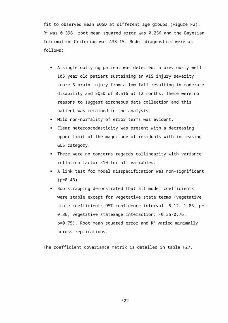
Figure H1. Pathophysiology of significant TBI

H.3.3 Treatment pathway conceptual model

Adults with suspected significant TBI can receive treatment in either SNCs or NSAHs, with the

location of the scene of injury, patient characteristics and underlying pathology influencing the

522

Primary brain injury

Focal injuries:Extradural haematomaSubdural haematomaIntracerebral haematomaIntracerebral contusion

Diffuse injuries:Diffuse axonal injuryCerebral oedema

Other intracranial injuries:Subarachnoid haemorrhageIntraventricular haemorrhageBrainstem lesionsLacerationsInfarction

Short Term Outcome:Death: secondary to TBI or its complications

Disability: Physical, Social, Cognitive, Psychological

Secondary brain injury

HypoxiaHypotensionHypoglycaemiaHyperpyrexiaMeningitisCNS infectionSeizuresHypocarbiaCoagulopathy

Raised intracranial pressure arising from:

HydrocephalusExpanding focal brain lesionsCerebral oedemaHypercarbiaSeizures

resulting in:Herniation syndromesCerebral ischemia

Injury factors Mechanism of injury: Blunt / penetrating / blast / crush Mode of injury: Isolated / multiple trauma Severity of insult

Patient factors Age Co-morbidites Ethnicity Genotype Medications Socieo-economic class

Long Term Outcome:•Death: Reduced life expectancy secondary to TBI or its complications;?

or reduced life expectacny due to characteristics associated with risk of TBI?Associated illnesses: Dementia, epilepsy, depressionsDisability: Physical, Social, Cognitive, Psychological

potential pathway of care. Potential management pathways were described in detail in

Chapter Two. Treatment pathways for patients with significant TBI are shown schematically in

Figure H2.

The factors determining the clinical effectiveness of the competing treatment pathways were

also discussed in Chapter Two. TBI management pathways are complex interventions with

several interacting factors influencing clinical effectiveness including: the timeliness of

important interventions (initial resuscitation, initiation of specialist intensive care, and

operative interventions in cases requiring neurosurgery); the relative efficacy of these

interventions when provided in NSAHs and SNCs; the potential for adverse events during

primary and secondary EMS transfers; and the potential for affecting patients with non-

significant TBI. Moreover, the relative importance of each of these determinants will vary

according to the actual underlying injury and the benefit of alternative management pathways

could conceivably vary across different TBI subgroups.[14-16]

523

Figure H2. Alternative management pathways for patients with suspected significant TBI

524

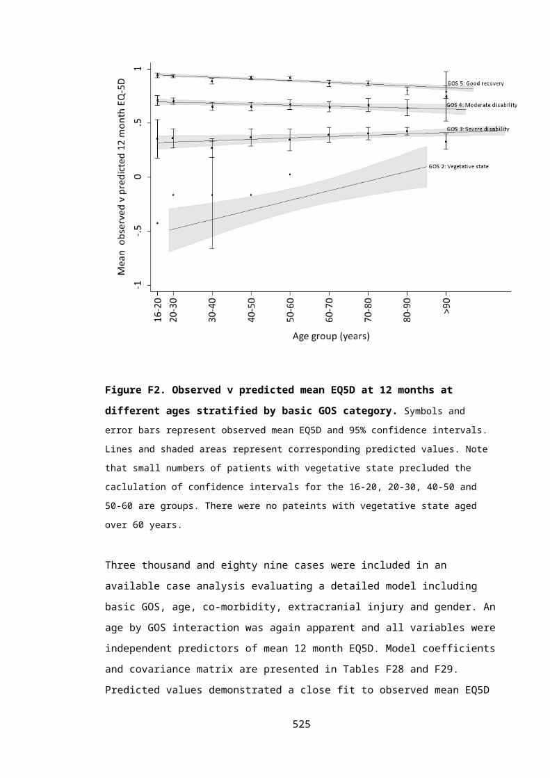
H.3.4 Design orientated conceptual model

From the disease logic and treatment pathway conceptual models was concluded that bypass

may improve outcomes by expediting definitive care for patients with suspected significant

TBI, but these benefits could be attenuated by non-compliance with bypass protocols, or offset

by a risk of prehospital deterioration and increased costs arising from more expensive

specialist management.

Explicit modelling of the effects of time to resuscitation and time to neurosurgery, using

prognostic models developed using TARN data, was pre-specified in the HITSNS study protocol.

However, during the model development process it was apparent that this was not a credible

approach. Literature reviews revealed no convincing evidence of an association between time

to treatment and outcome in TBI. Moreover relevant disability endpoints necessary to fully

represent outcome following TBI were not available within the TARN registry. [17] It had initially

been planned to impute GOS outcomes using data from a randomised controlled trial, the

Corticosteroid Randomisation After Significant Head Injury (CRASH) trial. [18] However, as time

to hospital arrival and critical care were not included in this dataset, and due to the limited

overlap of other covariates collected in TARN and CRASH, this approach was not feasible.

Furthermore, as reported in Chapter Four, when survival was examined using TARN data there

was no association observed between emergency services interval,[19] or time to neuroscience

centre care, and 30 day mortality; although in common with previously published studies in

this area interpretation of these findings is challenging due to high risk of bias. Access was

requested to other potentially suitable data sets to allow implementation of this approach,

including the RAIN study,[20] however no suitable data were available.

An analysis using existing data which reported no influence from earlier specialist care would

have had obvious results of no apparent difference in effectiveness, dubious face validity, and

was consequently redundant. As conceptual models clearly defined a strong theoretical basis

for potential differences in outcome between alternative management strategies it was

therefore necessary to override the flawed existing evidence in favour of the expert opinion of

the clinical community. A range of modelling methodologies and model structure were

subsequently carefully considered by the primary modeller and discussed in round table

meetings with the HITSNS advisory panel. Major challenges to model structuring that were

identified and examined in detail included: the unique HITSNS inclusion criteria with

consequent lack of empirical evidence to support model parameterisation; the very 525

heterogeneous population to which prehospital triage and bypass would apply and the

subsequent requirement for a wide range of evidence to parameterise any model; the

complexity of each management strategy with multiple potential treatment pathways

contributing to an overall pooled intervention-level outcome; and the need to model a wide

spectrum of potential outcomes ranging from perfect health to severe disability and death.

The possibility of directly modelling the effects of time to resuscitation and ICU treatment, and

explicitly including the risks and effects of secondary brain insults during bypass and inter-

hospital transfers, within an individual patient sampling model was particularly deliberated.

Such an approach, akin to that taken by Stevenson and colleagues (2002), [21] would entail

extensive elicitation of a large number of abstruse effect estimates, conditional on particular

combinations of treatment timings and patient characteristics. In contrast, the relative costs

and effectiveness of each management strategy compared with current practice were

considered to represent a more manageable number of tangible quantities that could be

credibly elicited from clinical experts. It was therefore decided to follow a similar approach to

that taken by the 2007 NICE head injury guideline group TBI economic model and use cohort

methodology to model each intervention at the strategy level. [22]

A hybrid cohort model was subsequently developed focusing on differences in outcomes and

costs with each management strategy for important patient sub-groups. [23] This design

orientated conceptual model did not differ from the final implemented model which was been

outlined in detail in Chapter Eight.

526

H.4 ASSUMPTIONS OF THE HITNS ECONOMIC MODEL

Decision analysis has been defined as ‘a systematic approach to decision making under

uncertainty’.[23] Models can provide an understandable, helpful and credible representation of

a complex and indecipherable reality. However it is important that the assumptions required

to achieve the inevitable simplification inherent in decision analysis models are transparent

and reasonable. This principle is captured by George Box’s aphorism that ‘essentially, all

models are wrong, but some are useful’.[24] The structural assumptions of the HITSNS model

are summarised in Table H2.

Table H2. HITSNS model assumptions

Model assumptions

Population

Adult patients with suspected significant TBI and initially stable

Setting

Strategies implemented in a geographical setting analogous to the HITSNS study

Perspective

NHS and personal social services

Treatment pathways

Outcomes for patients with mild TBI are independent of management strategy

Capacity in SNCs is unconstrained

Compliance with bypass is not related to prognosis in patients with mild TBI, expanding intra-cranial

haematomas, or TBI requiring ward care.

Introduction of prehospital triage and bypass would not result in de-skilling or disinvestment in

NSAHs. Patients inadvertently transported to NSAHs in a bypass strategy would therefore receive

comparable NSAH treatment as would be expected in secondary transfer strategies.

There is no correlation between costs and effects

Outcomes

Management strategies have no ongoing beneficial or detrimental effects on outcome beyond the

first year post-injury.

Long term disability in survivors of TBI remains constant, with no potential for improvement or

deterioration.

An additional QALY has the same weight regardless of the characteristics of the individuals receiving

the health benefit

Markov model

The death rate is equal across each year.

Frame of time preference

Positive frame of time preference with a 3.5% annual discount rate for costs and health effects

527

H.5 ECONOMIC MODEL SENSITIVITY ANALYSES

Table H3. Summary of sensitivity analyses

Sensitivity analysis Description Key parameters varied Alternative specification of model input*

Scenario analyses of parameter uncertainty:

Bypass: favourble

scenario

Cost-effectiveness of bypass when parameters set to

favourable, but still plausible values.

Relative effectiveness and

incremental costs for each patient

subgroup

0.25 and 0.75 quantiles of relevant parameter distributions

Bypass: unfavourable

scenario

Cost-effectiveness of bypass when parameters set to

unfavourable, but still plausible values.

Threshold analysis:

Bypass threshold analysis Incremental costs and relative effectiveness

parameters sequentially increased to identify

parameter values at which bypass becomes cost-

effective at λ=£20,000 and £30,000.


incremental costss for each patient

subgroup

Increasingly favourable 0.05 quantiles of relevant parameter

distributions

One-way sensitivity analyses of parameter uncertainty:

Population subgroups Alternative estimates for population subgroups. Dirichlet distribution for population

subgroups

Estimates used from each trial region, Dirichlet distribtutions:

NEAS: α1:87 α2:5 α3:16 α4:22 α5:9

NWAS: α1:8 α2:5 α3:3.5 α4:11 α5:0.5

Acute neurosurgery

baseline outcomes

Alternative estimates for outcomes of patients

requiring acute neurosurgery undergoing secondary

Dirichlet distribution for acute

neurosurgery (secondary transfer)

Dirichlet distribution derived from a published estimate (Taussky

2007)[25]

528

transfer. outcomes α1:18 α2:9 α3:27 α4:22

(posterior distribution after external bias adjustment)

Acute neurosurgery costs Alternative estimates for incremental costs of patients

requiring acute neurosurgery undergoing bypass.

Normal distribution for mean

incremental costs

No difference in costs except fixed transfer costs: -£200

Probabilistic analysis using published estimate (Fuller 2010),[26]

Normal distribution:

μ:9,880 SE:3,607

Incremental inpatient

costs for bypass

Alternative estimates for incremental inpatient costs

associated with bypass

Normal distribution for mean

incremental costs

Normal distributions elicited from clinical experts:

Mild TBI: μ:66 SE:8.6

TBI requiring ward care: μ:122 SE:250

TBI requiring critical care: μ:4000 SE:1200

TBI requiring acute neurosurgery: μ:3000 SE:1200

Major extracranial injury: μ:3120 SE:1260

Relative effectiveness for

major extracranial injury

patients

Alternative estimates for odds ratio for survival

following major extracranial injury associated with

bypass strategy

Normal distribution for log odds

ratio

Normal distribution elicited from clinical experts:

μ:-0.18 SD:0.05

GOS utilities Alternative estimates for utility values for GOS health

states based on published estimate

GOS utility values Alternative health states measured using scenarios and valued using

the standard gamble (Aoki 1998).[27] Utility decrement from perfect

health, Gamma distributions:

Dead: 1

Severe disability: α:33.1 β:0.03

Moderate disability: α:1.8 β:0.2

529

Good recovery: α:0.6 β:0.2

Alternative estimates for utility values for GOS health

states based on estimates derived using VSTR data

GOS utility values Alternative health states measured from patients with significant TBI

using the EQ5D and UK preference tariff: [Chapter 6]. Beta

distributions:

Dead: 1

Severe disability: α:594 β:939

Moderate disability: α:2437 β:1202

Good recovery: α:4496 β:534

Post discharge costs Elicited long term head injury costs evaluated. Post discharge costs for GOS states 0.25 quantiles of relevant distribution

One-way sensitivity analyses of structural uncertainty:

Alternative comparators Bypass with full compliance and no transfer (including

no transfer of patients requiring acute neurosurgery)

examined as potential strategies


incremental costs for TBI bypass and

no transfer strategies modified.

Normal distributions elicited from clinical experts for log proportional

odds/odds ratios:

Bypass - TBI requiring critical care: μ:-0.05 SE:0.41

Bypass - Major extracranial injury: μ:-0.30 SE:0.15

No transfer - TBI requiring neurosurgery: μ:1.0 SE:0.4 (applied to

baseline outcomes for delayed neurosurgery)

Discount rate Discount rates changed to explore different frames of

time preference

Discount rate Discount rate= 1.5% and Discount rate=6.0%

530

Proportional odds ratio Assumption of proportional odds effect on relative

outcomes removed.

Relative effectiveness for patient

subgroups of:

Acute neurosurgery

TBI requiring critical care

TBI requiring ward care

Odds ratio for unfavourable outcome applied, but the proportions of

patients in each constituent GOS category of the dichotomised

outcome group is equivalent to that observed in the baseline

outcome strategy.

Long term disability Assumption of static long term disability relaxed to

allow changes between GOS disability states post-

discharge

Distribution of GOS disability health

states in state transition model

Health state distribution modified at 6 and 12 years according to the

findings of Whitnall (2006) and McMillan (2012). Thereafter the

disability level is unchanged until death.

Long term survival Increased mortality in survivors of TBI and major

extracranial injury modelled.

Time dependency in state transition

model

Relative risk applied from literature applied to general population life

tables (McMillan 2011, Cameron 2005).[28, 29]

Increased mortality in survivors of TBI Time dependency in state transition

model

Transition probabilities derived from REP Gompertz model (Chapter

7)

Consideration of non-

health effects

Utility decrement applied to bypassed mild TBI

patients to account for inconvenience of unnecessary

transport to a distant hospital

Mild TBI outcomes in bypass

strategy

Utility decrement of 0.001

*All parameters treated probabilistically unless stated

531

H.6 EXPECTED VALUE OF INFORMATION

H.6.1 Background information on expected value of information analyses

To avoid potential opportunity costs health care systems should typically choose interventions

with the highest expected net monetary benefit, regardless of statistical uncertainty. [30, 31] This

approach will maximise health gains from available resources, and result in correct decision

making based on current evidence. However there is often considerable uncertainty in model

inputs and the optimal management strategy could differ if the true parameter values were

known with certainty. Any errors in the adoption decision will consequently result in forfeited

health benefits and wasted resources.

Economic models use probability distributions to reflect the uncertainty of a decision problem

and can simulate the entire spectrum of cost-effectiveness results that are possible given

potential realisations of parameter values. Assuming that these parameter distributions are

correctly specified, the probability of making the wrong adoption decision and the resulting

effects on costs and QALYs will therefore be available from implementing a probabilistic

sensitivity analysis. The opportunity losses surrounding a decision can consequently be

calculated for each patient by subtracting the maximum NMB resulting from a particular set of

parameter values from the mean expected NMB for the optimal strategy over the joint

distribution of all possible parameter values. As it is impossible to know exactly how the true

parameter values will resolve, it is necessary to average this calculation over all potential

resolutions of model inputs, by undertaking sufficient PSA runs.[23, 32] The resulting value is

termed the individual expected value of perfect information (EVPI), measuring the expected

cost of current uncertainty for each patient by accounting for both the probability that a

decision based on existing evidence is wrong and for the magnitude of the consequences of

making the wrong decision.[33] A rational decision maker should be willing to pay for additional

perfect evidence up to this level of expected opportunity loss, for the total population of

patients who may benefit from additional research evidence over the lifespan the technology,

a value known as the population EVPI.[33]

Population EVPI places an upper bound on any investment in future research, but does not

indicate what type of evidence would be valuable. By focusing attention on eliminating the

potential opportunity costs arising from uncertainty in particular model inputs expected value

of partial perfect information (EVPPI) can indicate research into which parameters would be

most valuable.[23, 34] Identification of variables where precise estimates would be most

532

important will indicate where research funds should be focused and may suggest appropriate

research designs. For example, a large EVPPI value for an estimate of relative effectiveness

would suggest a future randomised controlled trial is potentially useful; while a high EVPPI for

the prevalence of a disease subgroup could indicate an epidemiological cohort study.

Individual EVPPI, defined analogously to EVPI, is the expected net monetary benefit given

perfect information about the parameter of interest minus the expected NMB with current

information. Population EVPPI is similarly derived by multiplying the individual EVPPI by the

population of patients that would potentially benefit from additional information. Extension of

this technique to groups of parameters is possible using the same principles. [23]

Comparing the costs of future research studies against population EVPI and EVPPI provides a

necessary condition for future research: study costs must not exceed these values to be cost-

effective. However, they do not provide a sufficient condition that any future research study

will be helpful and cost-effective, and make the implausible assumption that all uncertainty

can be removed from a parameter value. Expected value of sample information (EVSI) extends

the value of information methodological framework to establish the expected value of

conducting studies with different designs and sample sizes.[34, 35] Individual EVSI is

mathematically defined as the expected difference between the value of the optimal decision

based on a sample of data, informative for certain model parameters, minus the value of

information based on existing evidence.[35] Population EVSI is computed equivalently to

population EVPI and EVPPI, but should account of the fact that patients recruited into a study

are ‘used up’ and cannot benefit from a study’s results, and that the length of a study may

reduce the time period an intervention is applicable.

The expected benefits of a given study sample (the population EVSI) can be compared with the

expected costs of collecting this data, with the difference denoting the expected net benefit of

sampling (ENBS). ENBS measures the societal reward from conducting additional research,

with ENBS greater than zero demonstrating that the marginal benefits of gathering further

evidence exceeds the marginal costs; and higher ENBS values representing more efficient study

designs. Optimal study designs can then be identified by choosing the largest ENBS from

different options with varying sample sizes, follow up periods, and study endpoints. [23]

533

H.6.2 Fixed and variable costs for a definitive HITSNS trial used in EVSI sensitivity analyses

Table H4. Assumptions for costs of a definitive HITNS trial used in ENBS sensitivity analyses

Assumptions in ENBS analysis

Base case value

Optimistic sensitivity

analysis

Pessimistic sensitivity

analysis

Envisaged HITSNS trial*

Information sources

Cost per recruited patient per year

£1,000 £500 £2,000 Fixed and variable

trial costs†

University of Sheffield CTRU, HITSNS grant application[36]

†Detailed in Table H5.

Table H5. Estimated fixed and variable trial costs for a definitive HITSNS trial based on the

HITSNS pilot study funding grant.

Trial resource Unit Cost Horizon

Fixed costs:University estate costs £43,000 -

Other university indirect charges £125,000 -

Office consumables £4,000 -

Project manager IT equipment £1,000 -

PR company to advertise trial £7,500 -

Conference attendance to promote trial and disseminate results

£5,000 -

Data management and security £15,000 -

Variable costs:

Principle investigator £12,000 per year

Trial manager £50,000 per year

Research paramedic £42,000 per ambulance service per year

Statistician £4,250 per year

Ambulance service advisor £2,500 per year

Other trial management group advisors £25,000 per year

Lease car £14,000 per research paramedic per year

IT equipment £850 per research paramedic

PR company to advertise trial £2,500 per ambulance service

Ambulance service training £12,500 per ambulance service

Ambulance service administrative support £750 per ambulance service per year

Trial manager travel and subsistence £1,000 per ambulance service per year

Trial management and other meetings £10,000 per year

Additional journey times for ambulances £100 per patient in intervention arm

Accessing patient notes £60 per patient

Patient leaflets, questionnaires and mailing costs £20 per patient

534

H.7 REFERENCES

1. Simoens S: Using the Delphi technique in economic evaluation: time to revisit the oracle? Journal of clinical pharmacy and therapeutics 2006, 31(6):519-522.

2. Dalkey NC, Brown BB, Cochran S: The Delphi method. Santa Monica, Calif.,: Rand Corp.; 1969.

3. Jones J, Hunter D: Consensus methods for medical and health services research. BMJ (Clinical research ed) 1995, 311(7001):376-380.

4. Linstone HA, Turoff M: The Delphi method : techniques and applications. Reading, Mass. ; London: Addison-Wesley; 1975.

5. Okoli C, Pawlowski SD: The Delphi method as a research tool: an example, design considerations and applications. Information & Management 2004, 42(1):15-29.

6. Powell C: The Delphi technique: myths and realities. Journal of advanced nursing 2003, 41(4):376-382.

7. Steurer J: The Delphi method: an efficient procedure to generate knowledge. Skeletal radiology 2011, 40(8):959-961.

8. Muthuri Kirigia J: Economic evaluation in schistosomiasis: using the delphi technique to assess effectiveness. Acta Tropica 1997, 64(3–4):175-190.

9. SmartSurvey [http://www.smartsurvey.co.uk/]10. Robinson S: Conceptual modelling for simulation Part I: definition and requirements.

. Journal of the Operational Research Society 2008, 59:278-290.11. Kaltenthaler E, Tappenden, P., Paisley, S., Squires, H.: Identifying and reviewing

evidence to inform the conceptualisation and population of cost-effectiveness models. . In: DSU Technical Support Documents. London: NICE 2011.

12. Werner C, Engelhard K: Pathophysiology of traumatic brain injury. British journal of anaesthesia 2007, 99(1):4-9.

13. Maas AI, Stocchetti N, Bullock R: Moderate and severe traumatic brain injury in adults. The Lancet Neurology 2008, 7(8):728-741.

14. Silver JM, McAllister TW, Yudofsky SC: Textbook of traumatic brain injury, 1st ed. edn. Washington, DC: American Psychiatric Pub.; 2005.

15. Maas AIR, Stocchetti N, Bullock R: Moderate and severe traumatic brain injury in adults. Lancet Neurology 2008, 7(8):728-741.

16. Moppett IK: Traumatic brain injury: assessment, resuscitation and early management. British journal of anaesthesia 2007, 99(1):18-31.

17. Trauma Audit and Research Network [www.tarn.ac.uk]18. Edwards P, Arango M, Balica L, Cottingham R, El-Sayed H, Farrell B, Fernandes J,

Gogichaisvili T, Golden N, Hartzenberg B et al: Final results of MRC CRASH, a randomised placebo-controlled trial of intravenous corticosteroid in adults with head injury-outcomes at 6 months. Lancet 2005, 365(9475):1957-1959.

19. Fuller G, Lawrence T, Woodford M, Coats T, Lecky F: Emergency medical services interval and mortality in significant head injury: a retrospective cohort study. European journal of emergency medicine : official journal of the European Society for Emergency Medicine 2014.


21. Stevenson MD, Oakley PA, Beard SM, Brennan A, Cook AL: Triaging patients with serious head injury: results of a simulation evaluating strategies to bypass hospitals without neurosurgical facilities. Injury 2001, 32(4):267-274.

535

22. Yates D, Aktar R, Hill J, Guideline Dev G: Guidelines - Assessment, investigation, and early management of head injury: summary of NICE guidance. Br Med J 2007, 335(7622):719-720.

23. Briggs AH, Claxton K, Sculpher MJ: Decision modelling for health economic evaluation. Oxford: Oxford University Press; 2006.

24. Box GEP, Draper NR: Empirical model-building and response surfaces. New York ; Chichester: Wiley; 1987.

25. Taussky P, Widmer HR, Takala J, Fandino J: Outcome after acute traumatic subdural and epidural haematoma in Switzerland: a single-centre experience. Swiss medical weekly 2008, 138(19-20):281-285.

26. Fuller G, Pattani H, Yeoman P: The Nottingham head injury register: A survey of 1,276 adult cases of moderate and severe traumatic brain injury in a British neurosurgery centre. Journal of the Intensive Care Society 2011(of Publication: January 2011):12 (11) (pp 29-36), 2011.




30. Claxton K: The irrelevance of inference: a decision-making approach to the stochastic evaluation of health care technologies. Journal of health economics 1999, 18(3):341-364.

31. Stinnett AA, Mullahy J: Net health benefits: a new framework for the analysis of uncertainty in cost-effectiveness analysis. Medical decision making : an international journal of the Society for Medical Decision Making 1998, 18(2 Suppl):S68-80.

32. Claxton K, Sculpher M, McCabe C, Briggs A, Akehurst R, Buxton M, Brazier J, O'Hagan T: Probabilistic sensitivity analysis for NICE technology assessment: not an optional extra. Health economics 2005, 14(4):339-347.

33. Eckermann S, Willan AR: Expected value of information and decision making in HTA. Health economics 2007, 16(2):195-209.

34. Claxton K, Posnett J: An economic approach to clinical trial design and research priority-setting. Health economics 1996, 5(6):513-524.

35. Ades AE, Lu G, Claxton K: Expected value of sample information calculations in medical decision modeling. Medical decision making : an international journal of the Society for Medical Decision Making 2004, 24(2):207-227.

36. Head Injury Straight to Neurosurgery Trial [http://www.hits-ns.tarn.ac.uk/]

536

I APPENDIX I: MODEL INPUTS FOR ECONOMIC MODEL EVALUATING ALTERNATIVE

MANAGEMENT PATHWAYS FOR ADULT PATIENTS WITH STABLE SUSPECTED

SIGNIFICANT TBI

I.1 INTRODUCTION

Parameterisation with unbiased model inputs is vital to ensure the validity of cost-

effectiveness models. NICE offers best practice guidance on the use of evidence to inform

health economic evaluations,[1, 2] recommending systematic reviews to identify relative

effectiveness estimates; and using systematic, reproducible and transparent methods for other

variables.

A wide variety of information sources were used for the parameterisation of the HITSNS model

including published and unpublished research, official reference sources, HITSNS pilot data,

trauma registry data, and expert opinion. Where relevant, findings from sub-studies conducted

during this PhD, and described in preceding chapters, have been used to specify mean values

and distributions for variables.

I.2 METHODS

I.2.1 Systematic reviews

Systematic review evidence was assessed to parameterise estimates of relative clinical

effectiveness between comparators for sub-groups of: i) patients with TBI requiring critical

care; and ii) patients with major extracranial injury. Selective secondary transfer was chosen as

the reference management pathway as this was current NHS practice when HITSNS was

conceived and had the greatest availability of baseline outcome data.

The systematic review evidence examining comparative effectiveness for patients with TBI

requiring critical care is described in Chapter Two. An additional search using identical

principles was performed to identify systematic reviews investigating patients with major

extracranial injury.

I.2.2 Literature reviews

NICE Decision Support Unit technical guidance on model parameterisation recognises that,

aside from clinical effectiveness data, formal systematic review methods are not feasible and

may be inappropriate for many model inputs.[2, 3] It acknowledges that search activities should

537

instead be tailored to the specific model parameter and focus on credibly populating the

economic model. Separate ‘rapid’ reviews were therefore performed to inform non-

effectiveness model inputs.[4] Searches aimed to identify sufficient evidence to achieve

information saturation, such that further efforts to identify more information would add

nothing to the analysis; and were based on the following principles:

A ‘systematic’ organised approach to identifying evidence

Transparency

Optimisation of searches for individual parameters

Balancing sensitivity with specificity and efficiency.

The primary information sources were established bibliographic databases (MEDLINE, EMBASE

and the Cochrane Library). Directed searching within these information sources promoted

satisfactory sensitivity. Additional high yield searching techniques were employed to increase

precision, including:

Utilisation of ‘rich patches’ including clinical experts, existing head injury economic

evaluations, established trauma registries, clinical guidelines, PubMed ‘Related

Citations’ and systematic reviews.

‘Snowballing’ with trails of cited references followed prospectively and retrospectively

from index sources.[5]

Internet searching using broad keyword strategies.

Inclusion of evidence indirectly retrieved in searches for related model parameters.

Identified evidence was reviewed for applicability to the HITSNS decision problem. Potentially

relevant data were then assessed for risk of bias using hierarchies of evidence,[6] appropriate

critical appraisal instruments,[7, 8] and theoretical considerations.[9-11] Only studies at low risk of

bias were considered to have met the minimum standard for inclusion in the model.

Searches were developed and performed by the primary modeller (GF). Assessment of

relevance and critical appraisal were also completed by the same investigator. Data were

collected for all potentially relevant studies using a generic form customised from the

Cochrane Collaboration.[12] Selected evidence was then additionally checked for

appropriateness by clinical experts in the HITSNS trial management group.

538

I.2.3 Expert elicitation

During evidence searching it was apparent that there were model inputs where no valid or

applicable data were available. Despite such weaknesses in the evidence base, a decision is still

necessary on which head injury management pathway to adopt. Clinical experts were

therefore asked to provide their beliefs on plausible values for parameters in formal elicitation

exercises.

Elicitation was performed using the Sheffield Elicitation Framework (SHELF), [13, 14] an

established methodology used in previous health technology assessments which includes

standardised documentation and computer software for distribution fitting. Ten out of a

possible 14 neuro-intensive care consultants at a regional UK SNC participated in elicitation of

relative effectiveness estimates for acute neurosurgery and patients with TBI requiring critical

care subgroups. The study sample was determined by experts’ availability on the day of the

elicitation exercise. All participants were sent comprehensive briefing material prior to the

elicitation session which included background information on: the HITSNS study; alternative

management strategies for suspected TBI; expert elicitation; and the SHELF framework.

References for further reading, and a contact telephone number and email address, were also

supplied to provide further information. For non-effectiveness variables where no valid data

were available, and for adjustment of indirectly relevant evidence, elicitation was performed

within the HITSNS trial management group.

The elicitation proceeded in five steps. Firstly, a detailed introductory session familiarised

experts with health economic modelling, probability distributions and expert elicitation.

Secondly, training exercises were performed where the elicitation of unrelated quantities was

practiced. Thirdly, background information and evidence relevant to each model input was

comprehensively reviewed and discussed. Fourthly, experts individually recorded their beliefs

on each parameter of interest. Finally, experts were provided with feedback on their chosen

probability distributions and a final consensus distribution was fitted following a group

discussion.

A probability histogram method was used by experts to represent their beliefs. The most

extreme plausible parameter limits were identified through group discussion and this range

was then divided into 10 equal intervals. Experts then distributed 20 ‘chips’, each indicating 5%

probability, across intervals to reflect their beliefs on the likelihood of alternative values.

Feedback was provided to each expert by presenting median values and 95% credible intervals

539

for the best fitting distribution to their probability histogram. A group distribution was then

fitted using the MATCH-2 internet application, summarising the responses of all 10 experts,

and presented to the group to provide a visual representation of collective opinion. [15] This

distribution was modified if necessary, informed by instant real-time modification of the

displayed distribution, after a round table group discussion. A final consensus distribution was

then confirmed with the group.

I.2.4 Incremental hospital costs

Representative patient level data were available for hospital resource use in each model sub-

group from HITSNS pilot study data. Incremental costs between patients initially transported

to NSAHs and SNC were subsequently calculated for each model population sub-group. The

study population comprised all eligible patients in the HITSNS trial with a prehospital GCS≤12,

with the subsequent study sample excluding patients with missing resource data due to lack of

identification, or refusal of consent. The HITSNS study protocol was modified prior to

commencement of recruitment with eligibility criteria in the NEAS region widened to a

prehospital GCS of ≤ 13 to give consistency with the coincidently introduced major trauma

bypass protocol. NEAS patients with GCS of 13 were excluded from the incremental cost

analysis to maintain compatibility with the modelled population.

Relevant data were collected for all major resource use categories, including transportation,

emergency department treatment, intensive care and ward admissions, operative procedures,

and inter-hospital transfers. Resources were valued in Pounds Sterling using NHS reference

costs and health care currencies.[16-19] Sub-classification of intensive care management by the

number of organ systems supported, as categorised in NHS reference costs, was not available,

and intensive care admissions were therefore assumed to correspond to the tariff for 3 organs

supported. The price base was 2012, with prices inflated to current values using Bank of

England consumer price index data where necessary.[20] Best practice trauma care tariffs were

applied for specialist care in patients with head injury requiring critical care, acute

neurosurgery and major extracranial injury.[19] Tariff increases associated with the provision of

specialist neuroscience care were also included for patients with significant TBI treated in

SNCs. Unit costs are presented in Table I1.

The distributions of cost data within each sub-group were initially assessed for normality by

visual inspection of frequency histograms. ‘As-treated’ complete case analyses of difference in

mean costs were then calculated. For sub-groups with low sample sizes (n<50) and non-normal

data non-parametric sampling with replacement was conducted,[21] using 2,000 bootstrap 540

replicates to determine the unadjusted mean incremental cost difference and associated

standard error between bypassed patients and those initially transported to NSAHs. In samples

with multiple patients from the same ambulance station, bootstrapped standard error

estimates were calculated accounting for clustering.

For sub-groups with larger sample sizes multi-level, random intercept, generalised linear

models were developed.[22] These models adjusted the mean incremental cost difference for

the potential confounders of age, prehospital GCS and injury severity score; and accounted for

clustering of cases within ambulance stations. Models were iteratively developed using the

Modified Park Test to assess the suitability of candidate families describing mean-variance

relationships; and goodness of fit statistics (Pearson’s correlation test and the Pregibon Link

Test) to tune the model link function.[23, 24] Mean incremental costs difference, with the

associated standard error and 95% confidence interval, were computed using the method of

recycled predictions and non-parametric bootstrapping.[23]

Analyses were performed in Stata version 12.1 (StataCorp, College Station, USA). The cluster

and strata options of the Stata bootstrapping command were used to account for clustering

where necessary. Multi-level models were implemented with maximum likelihood estimation

using the native xtmixed, and user written gllamm and glmdiag commands.[23, 25] Appropriate

regression diagnostics were performed to ensure the assumptions inherent in model

specifications were met. These included testing the distribution of random intercepts for

normality, assessing goodness of fit and examination of residuals.

541

Table I1. Inpatient unit costs for short term model

Cost Group Resource Measurement unit Price weight*(2012 price base)

Source

Transport Transportation to NSAH Single EMS transfer £316 Healthcare Financial Management Association[18]

Transportation to SNC Single EMS transfer £390 Healthcare Financial Management Association

Inter-hospital transfer Single EMS transfer £275 NHS reference costs[16, 19]

Emergency department care

ED payment by results tariff 1 Treatment episode £235 NHS reference costs





Neurosurgical operations

Intracranial procedures for trauma with diagnosis of head injury or skull fracture, with co-morbidities or complications

Per procedure £7,3836 NHS reference costs

Non-Neurosurgical operations†

Coronary artery bypass grafting Per procedure £7,358 NHS reference costs

Intermediate elbow and low arm procedure for trauma Per procedure £2,412 NHS reference costs

Major skin procedure category 1 Per procedure £1,881 NHS reference costs

Facial bones –plate Per procedure £1,973 NHS reference costs

Endscopic or intermediate general abdominal procedure Per procedure £1,462 NHS reference costs542

Exteriorisation of trachea without co-morbidity or complications

Per procedure £2,332 NHS reference costs

Intermediate Orbits procedure Per procedure £1,478 NHS reference costs

Overnight admission for observation

Overnight admission from ED for head injury observation Per admission £291 NHS reference costs

General ward admission**

General medical bed day Per day £252 RAIN study[26] / NHS reference costs

Intensive care admission (SNC)‡

Specialist intensive care bed day with 3 organs supported Per day £1470 RAIN study/ NHS reference costs

Intensive care admission (NSAH)‡

Non-specialist intensive care bed day with 3 organs supported

Per day £1464 RAIN study/ NHS reference costs

‘Top up’ payments Trauma best practice tariff: ISS>15 One-off payment £2,875 NHS reference costs

Trauma best practice tariff: ISS 9-15 One-off payment £1,495 NHS reference costs

Specialist neuroscience care uplift One-off payment 1.28 cost multiplier

NHS reference costs

*All unit costs inflated to a 2012 price base using Bank of England CPI data

† Some patients in the TBI requiring critical care, TBI requiring ward care and major extracranial subgroups had non-neurosurgical operations

** Weighted average of all categories of elective excess bed days.

‡ Separate unit costs extracted from payment by results database for NSAH and SNC critical care bed days (averaged over hospitals included in RAIN study).

543

I.2.1 Evidence synthesis

The identified evidence could be categorised into four groups. Firstly model inputs where a

single internally valid, directly relevant data source was available. This evidence was applicable

to the HITSNS decision problem in terms of patient groups and interventions, and could be

immediately applied in the model. Secondly, parameters where a single internally valid

evidence source was identified which was not directly applicable. Given the narrow and unique

inclusion criteria of the HITSNS study, adjustment to published estimates was necessary for

certain model inputs to allow generalisation to the modelled population. Beliefs about the

direction and magnitude of such ‘external biases’ were formally elicited and used to update

the prior evidence.[27] Thirdly, in cases where no valid or applicable evidence was available

elicited expert opinion was used to indicate the relative likelihood of plausible parameter

values. Finally, in the event of multiple eligible sources of evidence the final choice of base

case model input was based on weighing internal and external validity across available options,

with exploration of alternative input specifications in sensitivity analyses. Pooling of data was

also envisaged if homogenous data at low risk of bias was available. The evidence selected for

each model input is detailed and justified in the following sections. Further details on

information sources, search strategies, study details, critical appraisal and assessment of

applicability of evidence are available on request.

I.3 EVIDENCE FOR MODEL INPUTS

I.3.1 Population sub-groups

During the literature searches no studies were found with inclusion criteria consistent with the

HITSNS population. Estimates of the proportions of patients in each patient sub-group were

therefore based on a complete case analysis of HITSNS pilot study data, excluding non-TBI

patients with medical diagnoses. Each eligible patient with prehospital GCS≤12 was coded

according to injury, admission, treatment and neurosurgical characteristics and categorised

into one of the model’s five mutually exclusive sub-groups. Marked differences in the

composition of participants were evident between each HITSNS study region. A sensitivity

analysis was therefore performed using these separate estimates to investigate the influence

of case-mix on cost-effectiveness. Table I2 details the numbers of patients within each sub-

group.

544

Table I2. Proportion of patients within each modelled sub-group

Overall NEAS NWAS

Patient subgroup n Proportion point estimate (95% CI)

n Proportion point estimate (95% CI)

n Proportion point estimate (95% CI)

Mild TBI 95 0.57 (0.49-0.65) 87 0.63 (0.54-0.71) 8 0.30 (0.14-0.50)

TBI requiring ward admission

33 0.20 (0.14-0.27) 22 0.16 (0.10-0.23) 11 0.41 (0.22-0.61)


19 0.11 (0.07-0.17) 16 0.12 (0.07-0.18) 3 0.11 (0.02-0.29)

TBI requiring acute neurosurgery

10 0.06 (0.03-0.11) 5 0.04 (0.01-0.08) 5 0.19 (0.06-0.38)

Major extracranial injury

9 0.05 (0.03-0.10) 9 0.06 (0.03-0.12) 0 0.00 (0.00-0.13)

I.3.2 Baseline outcomes

Estimates of GOS at one year were necessary for the baseline selective secondary transfer

strategy in each patient subgroup. Unfortunately, such outcomes were unavailable from the

HITSNS study due to loss to follow up.

Patients with mild TBI

It was assumed that outcomes in this group were independent of prehospital level of

consciousness and vital signs i.e. such patients meeting HITSNS inclusion criteria represent a

random subset of all patients with mild TBI. A large randomised controlled trial (the OCTOPUS

study) was identified, comparing routine CT scanning to admission for observation following

mild head injury.[28] This study was performed in the Netherlands and measured self-reported

short term Glasgow Outcome Scale outcome at three months. As the original trial included

children outcomes for adult patients aged over 16 years were obtained from the study

authors, as shown in Table I3. No other relevant studies were found reporting appropriate GOS

data for this patient group.

Patients requiring acute neurosurgery

The acute neurosurgery subgroup was defined as patients where immediate emergency

neurosurgery was indicated, considered to predominantly represent patients with expanding

subdural and extradural haematomas. Literature searches did not find any studies reporting

545

short term disability outcomes for a population meeting HITSNS inclusion criteria, initially

treated in a NSAH and reflecting this mixture of pathologies. However, access was available to

data from the Nottingham Head Injury Register, a high quality prospective database of

consecutive moderate and severe head injury patients admitted to a SNC between 1995 and

2002.[29] The database collected 1 year GOS data and contained variables allowing the

definition of a population consistent with the modelled subgroup. One year outcomes for

patients initially admitted to a NSAH and undergoing secondary transfer and neurosurgery

within 12 hours for acute subdural and extradural haematomas are shown in Table I3.

Patients with TBI requiring critical care

For patients with TBI requiring critical care literature reviews revealed a single observational

study providing potentially relevant 6 month GOS results for the baseline selective secondary

transfer strategy (Harrison 2013).[26] However, the HITSNS eligibility criteria of stable

prehospital vital signs would be expected to result in relatively fewer patients with associated

extracranial injuries and less frequent secondary brain insults. The study’s authors were

contacted to request restricted outcome data for patients meeting HITSNS inclusion criteria,

but access to data was not provided. External bias adjustment was therefore performed to

account for the better outcomes anticipated in the modelled HITSNS population. An odds ratio

for differences in unfavourable outcome was elicited within the HITSNS trial management

group and applied to RAIN outcome estimates under a proportional odds assumption to

provide applicable baseline outcomes. In the proportional odds model the odds ratio can be

interpreted as a summary of the odds ratios obtained from separate binary logistic regressions

using all possible cut points of the ordinal outcome. Therefore, the single odds ratio is

constrained to be equal for each of the possible GOS cut points: 1 vs. 2,3,4; 1,2 vs. 3,4; and

1,2,3 vs.4, (vegetative state was not considered). Table I3 shows the published and adjusted

baseline outcomes for head injury patients requiring critical care. Figure I1 presents the

probability density function for the elicited adjustment odds ratio.

Patients with TBI requiring ward admission

For patients with head injury requiring admission to general hospital wards a single cohort

study was identified providing potentially relevant baseline disability data (McCartnan 2008).[30] This study reported post-discharge GOS for patients, excluding the elderly aged >65 years,

admitted to an Irish district general hospital, stratified according to head injury severity. Based

on patient demographics and intensity of inpatient care it was assumed that the reported mild

and moderate TBI strata corresponded to this model sub-group. External bias modelling using

546

a proportional odds ratio was again used to adjust outcomes to reflect HITSNS inclusion criteria

(Table I3 and Figure I1).

Figure I1. Elicited probability density plots for proportional odds ratios used to adjust

published baseline outcome data in critical care and ward admission sub-groups.

547

Table I3. Baseline GOS outcomes for NSAH care / selective secondary transfer strategy

GOS Category

Population subgroup Baseline comparator Parameter Good recovery

Moderate disability

Severe disability*

Death Source of estimate Time of outcome assessment

Mild TBI n 1430 95 89 9 OCTOPUS study[28] 3 months

Proportion(95% CI)

0.88(0.86-0.90)

0.06(0.05-0.07)

0.05(0.01-0.07)

0.006(0.003-0.01)

TBI requiring ward admission

Initially admitted to NSAH

n 163 7 2 0 McCartnan 2007[30] ‘Post discharge’ - undefined

Proportion(95% CI)

0.95(0.90-0.98)

0.04(0.02-0.08)

0.01(0.00-0.04)

0.00(0.00-0.02)

Posterior Dirichlet distribution†

84 6 2.5 3.5 Adjusted with expert opinion


Selective transfer n 174 198 262 216 RAIN study[26] 6 months

Proportion(95% CI)

0.20(0.18-0.23)

0.23(0.20-0.26)

0.31(0.28-0.34)

0.25(0.23-0.28)

Posterior Dirichlet distribution†

219 249 178 149 Adjusted with expert opinion

Acute neurosurgery Initially admitted to NSAH

n 20 19 12 38 NIHR database[31] 1 year

Proportion(95% CI)

0.22(0.14-0.33)

0.21(0.13-0.31)

0.13(0.07-0.22)

0.42(0.32-0.54)

*Severe disability category includes persistent vegetative state.

† Posterior distribution after updating published baseline outcomes with elicited proportional odds ratio accounting for differences in case-mix

548

Patients with major extracranial injury

In common with recent systematic reviews and scoping reports, no studies were found

describing short term GOS or disability outcomes in patients with major extracranial injury

treated with a selective secondary transfer strategy.[32, 33] Baseline outcomes were therefore

alternatively structured in terms of death and survival. The point estimate for mortality in the

small number of HITSNS patients with trivial head injuries but major extracranial injuries was

very imprecise (0.07, 95% CI 0.0-0.36, n=9). In preference, we interrogated the TARN database

between 2003 and 2010 to estimate mortality rates for cases meeting HITSNS inclusion

criteria. The calculated mortality risk was 0.035 (95% CI 0.033-0.036, n=48,681).

I.3.3 Relative effectiveness

Relative effectiveness estimates were unavailable from the HITSNS pilot study due to loss to

follow up secondary to non-consent, and external effect estimates were therefore required for

the following patient subgroups and treatment pathways:

TBI requiring ward admission: Bypassed patients compared with patients initially

transported to NSAHs.

TBI requiring critical care: All management strategies compared with selective

secondary transfer.

TBI requiring acute neurosurgery: Bypassed patients compared with patients initially

transported to NSAHs and undergoing secondary transfer.

Major extracranial injury: Bypassed patients compared with patients initially

transported to NSAHs.

Patients within the mild TBI sub-group were by definition deemed to be well enough for early

hospital discharge. It was therefore assumed that outcomes did not differ across strategies or

locations of care.

Relative effectiveness: TBI requiring ward care

No evidence was retrieved on the relative effectiveness of competing management strategies

for patients with TBI requiring ward admission. This subgroup may comprise patients with mild

to moderate head injuries, associated non-severe extracranial injuries (AIS injury severity

scores of 1 and 2), or medical co-morbidities. There could conceivably be small differences in

outcomes between patients managed in specialist and non-specialist centres secondary to

549

variations in treatment quality and access to rehabilitation services. We therefore elicited a

proportional odds ratio from clinical experts, as shown in Figure I2.

Relative effectiveness: TBI requiring critical care

As detailed in Chapter Two, two recent systematic reviews were identified which examined

management pathways for patients with TBI requiring critical care (Pickering 2014, Fuller

2013).[34, 35] Both of these reviews could only identify studies that were at very high risk of bias

and included populations that were not applicable to HITSNS decision problem. It was

therefore necessary to elicit relative effectiveness estimates from clinical experts. Figure I2

shows formally elicited odds ratios for differences in outcomes between selective secondary

transfer and other comparators, under a proportional odds assumption.

Relative effectiveness: acute neurosurgery

The foregoing systematic reviews did not identify any studies specifically examining a surgical

TBI subgroup. An additional detailed literature review focusing on the relative effectiveness of

bypass compared with secondary transfer strategies for patients requiring acute neurosurgery

was therefore performed, but did not retrieve any effect estimates suitable for inclusion in the

economic model. Seven observational studies, making some attempt to adjust for

confounding, were identified which compared outcomes in patients injured closest to a SNC

with patients transferred to neurosurgical units; or examined the effect of ‘early’ versus ‘late’

neurosurgery (Kim 2011, Kim 2009, Tien 2011, Hedges 2008, Tian 2008, Lee 1998, Howard

1989).[36-42] These studies reported conflicting results with 3 studies suggesting a benefit from

direct admission or neurosurgery within 4 hours, 1 study demonstrating a detrimental effect

and 3 studies reporting non-significant effects.

High risk of bias and limited generalisability prevented application of this evidence to the

HITSNS economic model. Confounding by indication was a critical threat to internal validity in

all studies. Other methodological flaws included high levels of loss to follow up (attrition bias),

inappropriately handled missing data (selection bias), retrospective collection of routinely

recorded clinical data (non-differential misclassification errors attenuating control of

confounding) and un-blinded outcome assessment (information bias). There were no

association evident between a study’s risk of bias and the direction and magnitude of the

reported effect estimates.

External validity was also lacking, with disability endpoints not collected. All studies included

patients injured closest to a SNC in the intervention group. Such patients will receive the

550

advantages of earlier definitive care, but will have less risk of deterioration and secondary brain

injury compared with those undergoing bypass. The majority of studies also investigated a

specific subset of cases, most commonly isolated subdural haematomas, rather than the

complete spectrum of pathologies requiring acute neurosurgery. The narrow inclusion criteria

of the HITSNS model’s population, with only attended by paramedics and initially stable

considered, also restricted applicability of the results of these studies. In the absence of

evidence relevant to the model we formally elicited an odds ratio for relative effectiveness

from clinical experts under a proportional odds assumption, as shown in Figure I2.

Relative effectiveness: major extracranial injury

A system level estimate of relative effectiveness was also required between bypass and the

selective transfer strategy baseline for the major extracranial injury subgroup. It was necessary

for this estimate to incorporate compliance with bypass, and account for secondary triage by

regional trauma centres. Furthermore, to allow generalisation to the model, the effect

estimate should be applicable to trauma cases meeting HITSNS inclusion criteria and exclude

patients with TBI.

Ideally, a pragmatic randomised controlled trial, with patients allocated randomly to bypass or

transport to the local NSAH, and examining disability endpoints, would be available to provide

unbiased estimates. Alternatively population based studies of regional trauma system

implementation, where comparable populations are treated under both strategies, could

provide indirect evidence. These study designs include controlled before and after studies,

controlled time series, interrupted time series and controlled studies of two or more

populations with and without trauma systems. However, these non-randomised designs would

usually be expected to study all patients within a trauma system, including patients injured

closest to trauma centres, and be at risk of confounding, potentially giving a less valid and

applicable effect estimate than a randomised controlled trial. Observational studies comparing

patients admitted to trauma centres with transferred patients will be unhelpful due to

confounding by indication, inclusion of directly admitted non-bypassed cases, and lack of

consideration of non-transferred cases.

Four systematic reviews (Mann 1999, Mullins 1999, Celso 2006, Davies 2014 - unpublished)

were identified which included observational population level trauma system evaluations. [43-46]

Two further detailed, but not fully systematic, rapid reviews were identified (Nicholl 2011,

Mcintosh 2013),[32, 33] of which one by Nicholl and colleagues included additional non-

randomised studies and re-analysed previously published population based data. Three

551

additional systematic reviews (Hill 2012, Williams 2013, Pickering 2014) were retrieved which

included observational studies comparing patients directly admitted to trauma centres to

patients initially admitted to NSAHs.[47-49] No randomised controlled trials were identified in the

available reviews; and included studies generally investigated patients with TBI within their

studied trauma populations and examined mortality as their only endpoint.

The systematic reviews by Mann 1999, Mullins 1999 and Celso 2006 were of variable quality,

and were confined to North American studies. The Celso review identified 14 population based

studies, questionably including 6 very heterogeneous effect estimates in a meta-analysis. From

these, two studies, by Mullins and colleagues (1998) and Nathens and Colleagues (2000), with

appropriately controlled designs and adjustment for case-mix were considered potentially

relevant to the HITSNS model.[50, 51] The preceding Mann 1999 and Mullins 1999 reviews

overlapped considerably and did not identify any additional relevant studies. The more recent

Nicholl 2011 rapid review did not use formal systematic methodology; employing a detailed

MEDLINE search which identified a further relevant study: Shafi 2006.[52] The other rapid

review by Macintosh and colleagues (2013), and the final systematic review of population

based studies by Davies (2014, unpublished), did not identify any further applicable studies.

The two systematic reviews (Hill 2012, Williams 2013) evaluating observational studies of

trauma centre effects were disregarded as they compared only directly admitted, non-

bypassed patients, with cases transferred into specialist centres. These studies cannot provide

valid system level estimates of outcomes. In the remaining systematic review by Pickering

2014 studies including patients initially admitted to NSAHs but not undergoing transfer were

also eligible. However, no studies were included reporting case-mix adjusted effect estimates

for a relevant study population.

Three original research studies were therefore initially considered for use in the economic

model (Shafi 2006, Nathans 2000, Mullins 1998). All reported superficially similar point

estimates for the relative effectiveness on mortality associated with trauma system care,

ranging from 0.8 to 0.95, with borderline or no statistical significance. However two of the

three studies calculated incident rate ratios as their effect estimate. The HITSNS economic

model is structured using probabilities and, as there can be substantial differences in the

association of an intervention with prevalent versus incident disease, risk ratios (or

equivalently odds ratios) are necessary to validly calculate relative outcomes between

strategies. The only study reporting a potentially usable effect estimate was therefore Mullins

1998, which reported an overall odds ratio of 0.80 (95% CI 0.70-0.91) for mortality associated

552

with trauma system care. However, this study used data from 1990-1993 and major trauma

care has evolved considerably in the last two decades. It also included patients with TBI and

enrolled patients outside of the HITSNS entry criteria. Furthermore, subgroup analyses

excluding TBI patients and examining different injury patterns indicated no clinically or

statistically significant benefit in orthopaedic, abdominal or thoracic trauma. Finally, only

inpatient mortality was studied, rather than the one year outcomes required in the short term

economic model. In response to these concerns we used the reported average odds ratio in

our base case model, but also elicited an odds ratio specific to the model’s scope for use in a

sensitivity analysis (Figure I2).

553

Figure I2. Elicited probability density plots for elicited estimates of relative effectiveness. Zero corresponds to no difference in effectiveness. Log proportional odds greater than

zero denote worse outcomes; values less than zero favour the reference management strategy.

554

I.3.4 Inpatient costs following TBI or major extracranial injury

Incremental costs between prehospital triage and bypass and selective secondary transfer

management strategies

Literature reviews failed to identify any published studies estimating incremental costs

between bypass and selective transfer strategies applicable to the economic model. A recent

systematic review by Humphreys and colleagues (2013) examining the costs of TBI highlighted

the paucity of data in this area, stating that there was ‘a lack of recent and substantial

evidence’ and ‘it is evident that past research seems inconsistent and prone to differing

methodological approaches’.[53] Moreover, identified data were almost exclusively from the US.

Representative patients enrolled in the HITSNS pilot study and consistent with the modelled

population were therefore studied in a programmatic cost analysis.

A total of 177 patients presented with GCS≤12, had complete data, and were classifiable into a

patient subgroup relevant to the model. Two patients with missing prehospital GCS, and

thirteen eligible patients who were unidentified or declined consent were excluded due to

missing data. Sample sizes for incremental costs within each subgroup varied from n=9 for

patients with major extracranial injury to n=95 for patients with mild head injury. The

derivation of the study sample is shown in Figure I3.

555

Figure I3. Derivation of the HITSNS study samples for cost analysis comparing transport to

NSAH with bypass to a SNC.

Although case-mix between bypassed and non-bypassed patients was broadly similar there

were some notable differences in potential confounders between study groups in certain

patient subgroups. Patients requiring acute neurosurgery and bypassed to SNCs were older

than cases taken to the nearest NSAH (median age 44 v 24 years). Conversely for the TBI

requiring ward care subgroup patients initially admitted to SNCs were much younger (median

age 49 v 77 years). Non-bypassed TBI patients requiring critical care demonstrated lower

prehospital oxygen saturations (median saturations 90 v 98%). Patient characteristics for each

subgroup are presented in Table I4.

556

Table I4. Patient characteristics or each model patient subgroup in cost analyses examining

mean incremental cost differences.

Patient characteristic Transported to NSAH

Transported to SNC

Mild TBI n=69 n=26

Age (years, median IQR) 43 (26-61) 33 (24-52)

ISS (median IQR) 1 (1-1) 1 (1-1)

PH GCS (median IQR) 11 (9-12) 12 (8-12)

PH sats (%, median IQR) 97 (96-98) 98 (96-98)

PH SBP (mmHg, median IQR) 131 (118-150) 140 (126-157)

EC injury (%, 95% CI) - -

TBI requiring acute neurosurgery n=6 n=4


ISS (median IQR) 26 (25-29) 25 (23-25)

PH GCS (median IQR) 5 (3-9) 3 (3-5)


PH hypotension mmHg, median IQR) 126 (113-127) 157 (124-167)

EC injury (%, 95% CI) 0 (0-46) 0 (0-60)

TBI requiring critical care n=7 n=12


ISS (median IQR) 16 (16-17) 20 (16-25)

PH GCS (median IQR) 9 (3-12) 6 (3-7)



EC injury (%, 95% CI) 0% (0-40) 17% (0-40)

TBI requiring ward care n=17 n=16


ISS (median IQR) 10 (1-20) 14 (1-25)

PH GCS (median IQR) 10 (7-12) 11 (6-12)



EC injury (%, 95% CI) 0 (0-20) 7 (0-20)

Major extracranial injury only n=2 n=7


ISS (median IQR) 13 (9-17) 9 (6-24)

PH GCS (median IQR) 3 (3-7.5) 3 (3-10)



EC injury (%, 95% CI) 100 100

Abbreviations: IQR: inter-quartile range; PH: prehospital; sats: pulse oximetry oxygen saturations; EC: extracranial

557

The distribution of costs was right skewed in all patient subgroups. The larger sample size for

mild head injury patients allowed development of multi-level models, adjusting for age and

prehospital GCS. An identity link and Gaussian family were selected as the most appropriate

specification based on model diagnostics. Unadjusted mean differences in cost, calculated

using non-parametric bootstrapping were used for other patient sub-groups. Incremental

mean cost differences are summarised for each sub-group in Table I5. A statistically significant

difference in mean cost was observed between patients with head injury requiring ward

admission initially transported to SNC compared with NSAHs (£2,353, 95% CI £414 - £4,291).

No other significant differences were apparent in other patient subgroups. The observed point

estimate for difference in costs for the acute neurosurgery subgroup undergoing bypass was

very large (£32,044, 95% CI £-3,722 - £67,811), however this result was very imprecise with the

95% confidence intervals being consistent with either increased or decreased mean costs.

Smaller point estimates for incremental differences in costs were observed in other patient

subgroups initially transported to SNCs: mild TBI (£68, 95% CI £-14 – £141), TBI requiring

critical care (£6,971, 95% CI £-21,840-£35,781), and major extracranial injury £5,922, 95%CI £-

4,433- £16,277).

Table I5. Mean cost differences between patients transported to NSAHs and SNCs

Patient subgroup Sample

size

Incremental mean cost

difference from NSAH care

95% confidence

interval

Mild TBI 95 £63 -£14 – £141

TBI requiring ward admission 33 £2,353 £414 - £4,291

TBI requiring critical care 19 £6,971 -£21,840 - £35,781

Acute neurosurgery 10 £32,044 -£3,722 – £67,811

Major extracranial injury 9 £5,922 -£4,433-£16,277

HITSNS estimates for incremental inpatient costs were very imprecise and considered to be of

borderline validity secondary to the potential risks of confounding and attrition bias. A

sensitivity analysis was therefore conducted based on the expert opinion of the trial

management group, using formally elicited parameter distributions, presented in Figure I4.

558

Figure I4. Elicited mean incremental inpatient cost differences between bypass and selective transfer strategies for each patient subgroup. Probability distributions elicited

within trial management group using SHELF elicitation framework.

559

Potentially relevant patient level data were also available from the Nottingham Head Injury

Register for the acute neurosurgery subgroup and was used in a further sensitivity analysis. [29]

The Nottingham Head Injury Register (NHIR) enrolled patients with moderate and severe TBI

admitted to the Queen’s Medical Centre, a UK SNC, between 1995 and 2002. The database has

been described in detail previously.[29] Briefly, directly admitted or referred patients

undergoing secondary transfer were prospectively included with a dataset of 636

demographic, clinical, treatment and injury variables collected from case notes and hospital

information systems. Outcome was measured by the basic GOS at one year using a structured

interview performed by each patient’s General Practitioner.

Patients were identified for inclusion in the cost analysis based on HITSNS eligibility criteria and

the presence of an extra-dural haematoma, subdural haematoma, or other intra-cranial

neurosurgical lesion undergoing operative management within 12 hours of injury. Health

service resource use was then measured and valued for each case using NHS reference costs as

described previously. A multivariable generalised linear model was subsequently developed

with total inpatient cost as the dependent variable, treatment pathway (direct admission or

secondary transfer) as an independent variable, and the potential confounders of age, GCS and

pupil responses as further explanatory variables. Models were developed iteratively using the

Modified Park Test and goodness of fit statistics to optimise their specification.[23] Mean

incremental costs difference, with the associated standard error and 95% confidence interval,

were then computed using the method of recycled predictions and non-parametric

bootstrapping.

The NHIR enrolled a total of 1,662 patients, of whom 1,276 were adults. From these 113

patients met HITSNS inclusion criteria and were classified as requiring acute neurosurgery.

Ninety four cases were initially admitted to a NSAH and underwent secondary transfer to the

SNC, 32 patients were directly admitted to the SNC. No cases were excluded due to missing

data. Case mix between directly admitted and referred patients was similar (Table I6).

Although cost data were right skewed a generalised linear model with an identity link and

inverse Gaussian family was found to be appropriate based on model diagnostics. Directly

admitted patients demonstrated higher costs than referred patients, with a mean incremental

cost difference of £9,880 (95% CI £2,811 - £16,950).

560

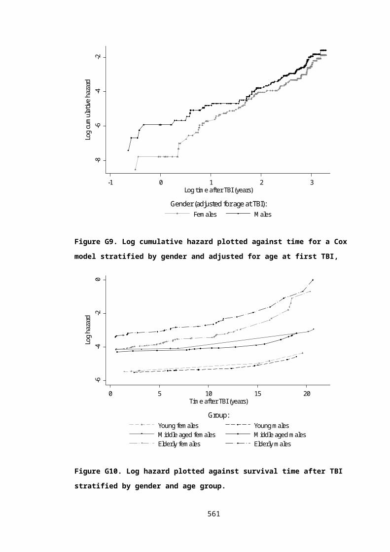
Table I6. Characteristics of directly admitted and referred patients requiring acute

neurosurgery in the Nottingham Head Injury Register.

Patient characteristic Secondary transfer from

NSAH

Direct admission to NC

94 32


ISS (median IQR) Not available Not available

ED GCS (median IQR) 7 (4-9) 6 (4-10)

ED pupils (% abnormal, 95% CI) 19 (11-29) 21 (8-41)

ED sats (%, median IQR) 98 (94-99) 98 (94-99)

ED SBP (mmHg, median IQR) 140 (135-163) 150 (135-163)

EC injury (%, 95% CI) Not available Not available

Incremental cost difference between selective secondary transfer and routine/no secondary

transfer strategies

Estimates for differences in mean inpatient cost were also required between selective

secondary transfer and routine and no transfer strategies for patients with TBI requiring critical

care. No studies were identified providing such data. The RAIN study reported adjusted

incremental costs between no-transfer and routine transfer strategies,[26] but in addition to

examining a different baseline comparator, this estimate also included post-discharge costs

and was averaged over all patients with TBI regardless of their prehospital vital signs. It was

therefore necessary to elicit incremental costs, informed by the RAIN and HITSNS results, from

the HITSNS trial management group. Elicited distributions are presented in Figure I5.

561

Figure I5. Elicited probability density plots presenting elicited expert opinion on mean

incremental costs between competing secondary transfer strategies for patients TBI

requiring critical care.

I.3.5 Post discharge and long term costs following TBI and major extracranial injury

Post discharge costs following TBI

A literature review of post-discharge costs for TBI patients whose outcomes are represented

by GOS states revealed only one relevant information source. This study, by Beecham and

colleagues (2008), evaluated the costs of health and social care services used by young British

adults aged 18-25 years presenting to emergency departments with an acquired brain injury,

predominantly head injury.[54] Literature reviews, resource databases, expert opinion and

national surveys were used to estimate the incidence of acquired brain injuries, define care

pathways and assess the level of health service in the first year following injury. Resource use

was then valued using 2006 NHS reference costs. The study estimated costs per patient

categorised into four groups corresponding closely to the modelled GOS health states. Only

point estimates of yearly costs were presented and in order to represent uncertainty in these

estimates standard errors and 95% confidence intervals were calculated under the assumption

that the standard deviation was equal to the mean for each GOS category. Given the paucity of

literature in this area it was also assumed that the reported costs for young adults were

representative of the mean post-discharge costs of all TBI survivors, and that patient who died

562

within the first year accrued no post-discharge costs. Reported costs, adjusted for CPI inflation,

are shown in Table I7.

Table I7. Mean first year post-discharge cost for head injury survivors, classified by GOS

category.

GOS Category Point Estimate of mean cost 95% confidence interval

Good recovery £413 £410 - £415

Moderate disability £29,507 £26,416 - £32,599

Severe disability £58,292 £51,803.07 - £64,781

Dead £0 £0 - £0

Long term costs following TBI

No UK studies were found examining longer term costs beyond the first year post-injury

applicable to GOS health states TBI survivors. Estimates were available from previous US cost-

analyses and health economic models (Leibson 2012, Faul 2007, Finkelstein 2006). [55-57]

However, given the lack of comparability between health care systems, and the aggregated

inclusion of productivity costs, these estimates were not considered generalisable to the

model’s NHS context. Annual long term costs, beyond the first year post head injury, were

therefore formally elicited within the HITSNS trial management group after reviewing the

available short term UK data and longer term US evidence. Elicited costs are shown in Figure

I6.

563

Figure I6. Elicited probability distributions for long term annual costs following head injury,

classified by GOS category.

Post-discharge and long term costs following major extracranial injury

A large UK study was identified reporting directly relevant data for post-discharge and longer

term costs following major extracranial injury. The HALO study prospectively investigated a UK

cohort of accidently injured casualties derived from 5 studies conducted between 1997 and

2003.[58] All studies included details of NHS resource use from hospital discharge to six months

post trauma. A sample of survivors was also surveyed an average of 9.5 years (4 to 15 years)

post injury and asked for details of resource use related to their initial injury over the

preceding year. Unit costs were valued using NHS reference costs and price weights from the

Personal and Social Services Research Unit. The mean cost in the first year following injury was

£7,884 (95%CI £7,697–£8,072, n=6,788, inflated to 2012 prices, standard deviation assumed to

the same as the mean value). Annual long term mean costs were £412 (95% CI £369 - £467,

n=545, standard deviation assumed to equal mean).

564

I.3.6 Preference weights for modelled health states

HSPWs for GOS categories

A systematic review, fully reported in Chapter Six, was conducted to identify available HSPWs

for GOS categories. Five eligible studies were identified,[59-63] of which one study approximated

the NICE reference case for utility data (Smits and colleagues, 2010).[60] These estimates have

been used in a recent TBI economic evaluations,[60, 64] including NICE Health Technology

Assessment submissions,[64] and were therefore included in the base case to maximise the

comparability of results. Other retrieved studies were less suitable, deriving utility values using

case scenarios and valuing the preferences of medical professionals or unrepresentative

general public samples. Despite these limitations the estimates provided by Aoki and

colleagues (1998) have been used extensively in TBI health economic models and they were

therefore examined in a sensitivity analysis to investigate the influence of alternative utility

values on cost-effectiveness results.[63, 65-69]

As no utility values for GOS health states were available that were fully compatible with the

NICE reference case a novel mapping study was performed to estimate preference weights

from a sample of patients with significant TBI using the EQ5D generic utility instrument and UK

preference tariff. These analyses are fully detailed in Chapter Six and results were used in a

further sensitivity analysis.

HSPWs for survivors of major extracranial injury

A literature review targeting studies providing utility data consistent with the NICE reference

case for survivors of major extracranial injury identified only the HALO study as providing

relevant evidence.[58] Health related quality of life was measured at 6 months (SF-36 and

Nottingham Health Profile), and between 4 and 15 years (EQ5D), post injury. Utility at six

months was calculated from predicted EQ5D scores using a mapping function based on linear

regression of domain level SF-36 or Nottingham Health Profile responses, and patient

characteristics. Six month HALO utility estimates were used for survivors of major extracranial

injury in the short term model (mean utility 0.67, SE 0.01). As later HALO estimates of utility

were virtually identical (mean utility value at 5 years 0.68, SE 0.03) the six month estimate was

also used to value health states in the base case long term Markov model.

565

I.3.7 Prognosis following TBI and major extracranial injury

Long term survival following TBI

All previously reported economic models in TBI have used the cross-sectional mortality

experience of the general population to model long term survival following TBI. To increase

comparability these estimates were also used in the HITSNS base case model. Contemporary

single-sex period life tables for England and Wales from the year 2012 were combined to

construct a person-level life table using methodology consistent with the UK Office of National

Statistics.[70] The radix of gender specific published life tables were adjusted according to the

UK ratio of 105.1 male births to 100 females. The numbers remaining alive at each age of life

(lx|male and lx|female), and the number dying each year (dx|male and dx|female), were then calculated

separately for each resulting gender birth cohort by applying the appropriate sex-specific

yearly probabilities of death (qx|male and qx|female). Dividing the resulting total number of deaths

each year (dx|male + dx|female), by the total males and females alive at each age (lx|male + lx|female)

computed the conditional probability of dying each year for the total general population.

These conditional probabilities were then directly applied as transition probabilities in the long

term Markov model.

A detailed literature review, described in Chapter Seven, identified 10 studies investigating

long term survival following TBI in unique patient cohorts (Brown 2013, Baguley 2012,

Himanen 2011, McMillan 2011, Ventura 2010, Harrison-Felix 2009, Cameron 2008, Colantonio

2008, Ratcliff 2005, Shavelle 2001).[70-79] Increased long term mortality was universally reported

for patients hospitalised following TBI, compared with the general population or non-TBI

community controls. Sensitivity analyses investigating the potential influence of decreased life

expectancy in survivors of TBI were therefore also implemented. Retrieved studies were

designed from an epidemiological viewpoint to determine the isolated effect of TBI on survival,

rather than extrapolate the future life expectancy of typical patients with TBI. The reported

effect estimates (standardised mortality ratios, odds ratios, relative risks, or rate ratios),

controlling for associated demographic and injury characteristics, therefore required further

adjustment to allow application to the long term Markov model.

McMillan and colleagues (2010) compared mortality over 13 years in a large British cohort of

TBI survivors to community non-TBI controls matched for age and socioeconomic status. [74]

This study sample was considered to be most representative of the HITSNS population from

the available published TBI cohorts. For cases surviving beyond the first year of follow up the

relative risk of death during follow up was 2.13 (95%CI 1.75-2.60, n=1,421). This estimate was 566

used to adjust the general population period life table and produce a survival curve reflecting

the higher risk of mortality following TBI.

Probabilities are non-linear functions of time and relative risks are consequently specific to the

time period over which they are calculated. It is therefore not appropriate adjust baseline

Markov model transition probabilities with relative risks calculated over a different time

period. Consequently the method reported by Price and colleagues (2009) was used to adjust

McMillan’s reported 13 year relative risk to that required for application to the 1 year cycle

length of the HITSNS economic model.[80] The following equation was used:

Where:

RR = Relative risk of event

c = Cycle length defining transition probabilities

Pb= Probability of event in group of interest

Pa= Probability of event in control group

s= Length of time period over which probabilities Pa and Pb are defined

The adjusted relative risk derived from McMillan 2010 (RRc=2.77) compares patients with

TBI to those without TBI. This estimate is not directly applicable to the general population life

table which provides survival estimates for a given age, averaged over all citizens, including

those who have already sustained a TBI. The method proposed by Pharoah and Hollingworth

(1996) was consequently used to calculate a ‘scale up factor’, adjusting general population

annual transition probabilities (qx) to account for the relative risk of those with and without

TBI, and the prevalence of TBI within the general population.[81, 82] The following equation was

used:

Where:

θ = The ‘scale up factor;

r = relative risk of event (specific to markov model cycle length and time period of life table)

p = prevalence of disease567

As previously noted there is an absence of UK studies investigating the adult prevalence of TBI,

an estimate from an internally valid New Zealand study by Feigin and colleagues (2013), which

followed a birth cohort into adulthood, was therefore used. [83] The final scale up factor for risk

of death (θ=1.78) was assumed to be constant over time and was applied to person level life

tables with adjusted state transition probabilities consequently derived.

Given the uncertainties surrounding the scaling of general population period life table data

using adjusted published effect estimates, an original study using parametric survival analysis

to quantify survival following TBI was also conducted, previously described in Chapter Seven.

The conditional probabilities that an individual sustaining a TBI at age 50 would survive each

subsequent year were calculated with the final Gompertz parametric model using post-

estimation commands from the streg module in Stata version 12.1 (StataCorp, College Station,

USA). The results of this study were unavailable until after model implementation and the

values were therefore included in a further sensitivity analysis.

Long term survival following major extracranial injury

The literature examining life expectancy following major extracranial injury is limited with only

two relevant studies reporting conflicting results identified. Evidence from the previously

described HALO study suggests that life expectancy in survivors of severe trauma returns to

that of the general population approximately six months after injury, although this result is at

relatively high risk of systematic error from attrition bias.[58] Conversely, a study by Cameron

and colleagues (2005),[77] investigating a representative sample of Canadian patients

hospitalised with non-head injuries, reported decreased long term survival. Transition

probabilities based on general population life tables were therefore used in the base case

time-dependent Markov model, with a sensitivity analysis implemented to investigate the

effects of a putative increase in mortality rates. A crude risk ratio of 1.68 (95% CI 1.50-1.88) for

mortality between 2 and 10 years post-injury was calculated from data reported by Cameron

2005 (n=26,316).[77] This relative risk was modified to account for the one year cycle length in

the HITSNS Markov model, and then used to in conjunction with a prevalence estimate for

adult major trauma provided by Lecky and colleagues (2010) to calculate a ‘scale up factor’. [84]

The final ‘scale up factor’ (θ=1.83) was again assumed to be constant throughout survival

following trauma and applied to yearly general population life-table death probabilities to

determine Markov model transitions.

568

I.4 FINAL INPUTS FOR HITSNS ECONOMIC MODEL

Table I8. Deterministic values and probability distributions for HITSNS economic model inputs

Model input Deterministic value Parameter type and distributional form

Distribution parameters for PSA*

Information source

Population subgroupsMild TBI 0.57 Proportion, Dirichlet α1: 95 HITSNS pilot data[85]

Acute neurosurgery 0.06 α2: 10TBI requiring critical care 0.11 α3: 19TBI requiring ward admission 0.20 α4: 33Major extracranial injury 0.05 α5: 9Compliance with bypass**Mild TBI 0.35 Proportion, Beta α:22 β:41 HITSNS pilot dataAcute Neurosurgery 0.83 Proportion, Beta α:2.5 β:0.5 HITSNS pilot dataTBI requiring ward care 0.57 Proportion, Beta α:12 β:9 HITSNS pilot data

Mild TBI outcomesDead 0.01 Proportion, Dirichlet α1: 9 OCTOPUS study[28]

Severe disability 0.05 α2: 89Moderate disability 0.06 α3: 95Good recovery 0.88 α4: 1430

Acute neurosurgery baseline outcomes (secondary transfer)Dead 0.41 Proportion, Dirichlet† α1: 36 NHIR study[31]


TBI requiring critical care baseline outcomes (selective transfer)

569

Dead 0.19 Proportion, Dirichlet† α1: 149 RAIN study[26]


TBI requiring ward care baseline outcomes (selective transfer)Dead 0.03 Proportion, Dirichlet† α1: 3.5 McCartan 2007[30]

Severe disability 0.02 α2: 2.5Moderate disability 0.06 α3:6Good recovery 0.88 α4: 84

Major extracranial injury baseline outcomes (selective transfer)

Survival 0.96 Proportion, Beta α:1690 β:46991 TARN database[86]

Relative effectiveness (v selective secondary transfer, proportional odds ratio for unfavourable outcome)Bypass: Acute neurosurgery 0.53 Log odds ratio, Normal μ:-0.68 SE:0.34 Expert opinionBypass: TBI requiring critical care 1.00 Log odds ratio, Normal μ:0.0 SE:0.41 Expert opinionBypass: TBI requiring ward care 0.98 Log odds ratio, Normal μ:-0.01 SE:0.02 Expert opinionBypass: Major extracranial injury 0.80 Log odds ratio, Normal μ:-0.22 SE:0.07 Mullins 1998[51]

Routine transfer: TBI requiring critical care 0.86 Log odds ratio, Normal μ:-0.15 SE:0.12 Expert opinionNo transfer: TBI requiring critical care 2.14 Log odds ratio, Normal μ:0.76 SE:0.35 Expert opinion

Inpatient costs (v selective transfer, incremental mean cost)Bypass: Mild TBI £63 Mean difference, Normal μ:63.3 SE:39.7 HITSNS pilot dataBypass: Acute neurosurgery £32,044 Mean difference, Normal μ:32,044 SE:18,249 HITSNS pilot dataBypass: TBI requiring critical care £6,971 Mean difference, Normal μ:6,971 SE:14,699 HITSNS pilot dataBypass: TBI requiring ward care £2,353 Mean difference, Normal μ:2,353 SE:981 HITSNS pilot dataBypass: Major extracranial injury £5,922 Mean difference, Normal μ:5,922 SE:5,283 HITSNS pilot dataRoutine transfer: TBI requiring critical care £7,500 Mean difference, Scaled Beta α:3.66 β:4.00 Max:10,000

Min:5,000Expert opinion

No transfer: TBI requiring critical care -£7,500 Mean difference, Scaled Beta α:3.66 β:4.00 Max:-10,000 Min:-5,000

Expert opinion

570

Short term post discharge costs (mean cost first year post injury)Dead £0 - - -Severe disability £58,292 Mean costs, Normal μ:58,292 SE:3,311 Beecham 2009[54]

Moderate disability £29,507 Mean costs, Normal μ:29,507 SE:1,577 Beecham 2009Good recovery £413 Mean costs, Normal μ:413 SE:1.31 Beecham 2009Survival from extracranial injury £7,884 Mean costs, Normal μ:7,884 SE:338 HALO study[58]

Long term post discharge costs (mean annual costs subsequent years)Dead £0 - - -Severe disability £12,500 Mean cost, Beta α:4.93 β:6.14 Expert opinionModerate disability £1,600 Mean cost, Lognormal μ:7.59 SD:0.36 Expert opinionGood recovery £24 Mean cost, Beta α:1.54 β:5.81 Expert opinionSurvival from extracranial injury £413 Mean cost, Normal μ:7884 SE:338 HALO study

Health state preference weights‡Dead 0 - - -Severe disability 0.15 Mean utility decrement from

perfect health, Gammaα:164 β:0.01 Smits 2010[60]

Moderate disability 0.51 Mean utility decrement from perfect health, Gamma

α:64 β:0.01 Smits 2010

Good recovery 0.88 Mean utility decrement from perfect health, Gamma

α:6.8 β:0.02 Smits 2010

Survival from extracranial injury 0.67 Mean utility, Beta α:3022 β:1475 HALO study

Notes:

*Continuity correction applied for Beta and Dirichlet distributions with parameter values<5. **Compliance with bypass was not directly modelled for patients with TBI requiring critical care or major

extracranial injury cases. The effect of compliance was incorporated within estimates of relative effectiveness for these subgroups. † Posterior distribution after external bias adjustment. ‡ Utility

values were subsequently adjusted for age in the Markov model using a multiplicative model based on comparative mean EQ5D values in the general population.

571

I.5 REFERENCES

1. Health Technology Assessment (HTA) Programme [http://www.nets.nihr.ac.uk/programmes/hta]

2. Kaltenthaler E, Tappenden P, Paisley S: Reviewing the Evidence to Inform the Population of Cost-Effectiveness Models within Health Technology Assessments. Value in Health 2013, 16(5):830-836.

3. Kaltenthaler E, Tappenden, P., Paisley, S., Squires, H.: Identifying and reviewing evidence to inform the conceptualisation and population of cost-effectiveness models. . In: DSU Technical Support Documents. London: NICE 2011.

4. Khangura S, Konnyu K, Cushman R, Grimshaw J, Moher D: Evidence summaries: the evolution of a rapid review approach. Systematic reviews 2012, 1:10.

5. Greenhalgh T, Peacock R: Effectiveness and efficiency of search methods in systematic reviews of complex evidence: audit of primary sources. BMJ (Clinical research ed) 2005, 331(7524):1064-1065.

6. Concato J, Shah N, Horwitz RI: Randomized, controlled trials, observational studies, and the hierarchy of research designs. The New England journal of medicine 2000, 342(25):1887-1892.

7. Katrak P, Bialocerkowski AE, Massy-Westropp N, Kumar S, Grimmer KA: A systematic review of the content of critical appraisal tools. BMC medical research methodology 2004, 4:22.

8. Higgins JPT, Altman DG, Gotzsche PC, Jueni P, Moher D, Oxman AD, Savovic J, Schulz KF, Weeks L, Sterne JAC et al: The Cochrane Collaboration's tool for assessing risk of bias in randomised trials. Br Med J 2011, 343.

9. Elwood JM: Critical appraisal of epidemiological studies and clinical trials, 3rd ed. edn. Oxford: Oxford University Press; 2007.

10. Szklo M, Nieto FJ: Epidemiology : beyond the basics, 2nd ed. edn. Sudbury, Mass.: Jones and Bartlett Publishers; 2007.

11. Rothman KJ, Greenland S, Lash TL: Modern epidemiology, 3rd ed. edn. Philadelphia, Pa. ; London: Lippincott Williams & Wilkins; 2008.

12. Higgins J, Green SP: Cochrane handbook for systematic reviews of interventions. Oxford: Wiley-Blackwell; 2008.

13. O'Hagan A: Uncertain judgements : eliciting experts' probabilities. Chichester: Wiley; 2006.

14. SHELF: the Sheffield Elicitation Framework [http://www.tonyohagan.co.uk/shelf/]15. Morris DE, Oakley JE, Crowe JA: A web-based tool for eliciting probability

distributions from experts. Environmental Modelling & Software 2014, 52(0):1-4.16. Health Do: NHS Reference Costs 2011/2012. In. London: DoH; 2012.17. Health Do: NHS Reference costs 2007/2008. In. London: DoH; 2008.18. Association. HFM: Payment by results for Ambulance Services.. In. London: HFMA; 2008.19. Health Do: NHS Payment by Results Guide 2012/2013. In. London: DoH; 2013.20. Consumer Price Indices

[http://www.ons.gov.uk/ons/rel/cpi/consumer-price-indices/index.html]21. Barber JA, Thompson SG: Analysis of cost data in randomized trials: an application of

the non-parametric bootstrap. Statistics in medicine 2000, 19(23):3219-3236.22. O'Connell AA, McCoach DB: Applications of hierarchical linear models for evaluations

of health interventions: demystifying the methods and interpretations of multilevel models. Evaluation & the health professions 2004, 27(2):119-151.

23. Glick H: Economic evaluation in clinical trials. Oxford: Oxford University Press; 2007.24. Manning WG, Mullahy J: Estimating log models: to transform or not to transform?

Journal of health economics 2001, 20(4):461-494.

572

25. Rabe-Hesketh S, Skrondal A, Pickles A: Generalized multilevel structural equation modeling. Psychometrika 2004, 69(2):167-190.


27. Turner RM, Spiegelhalter DJ, Smith GCS, Thompson SG: Bias modelling in evidence synthesis. Journal of the Royal Statistical Society: Series A (Statistics in Society) 2009, 172(1):21-47.

28. af Geijerstam JL, Oredsson S, Britton M: Medical outcome after immediate computed tomography or admission for observation in patients with mild head injury: randomised controlled trial. BMJ (Clinical research ed) 2006, 333(7566):465.

29. Fuller G PH, Yeoman P. : The Nottingham Head Injury Register: a Survey of 1,276 Adult cases of Moderate and Severe Traumatic Brain Injury in a British Neurosurgery Centre. . Journal of Intensive Care Society 2011, 12(1):1-7.

30. McCartan DP, Fleming FJ, Motherway C, Grace PA: Management and outcome in patients following head injury admitted to an Irish Regional Hospital. Brain injury : [BI] 2008, 22(4):305-312.

31. Fuller G, Pattani H, Yeoman P: The Nottingham head injury register: A survey of 1,276 adult cases of moderate and severe traumatic brain injury in a British neurosurgery centre. Journal of the Intensive Care Society 2011(of Publication: January 2011):12 (11) (pp 29-36), 2011.

32. Nicholl J YT, Pickering A, Turner J, Goodacre S.: The cost-effectiveness of regional networks for major trauma in England. . In.: School of Health and Related Research, University of Sheffield.; 2011.

33. Scotland. HI: What is the evidence for the clinical and cost-effectiveness of major trauma centres as the core component of a trauma service, compared with standard care for adults with major trauma? . In: Technologies Scoping Report. 2013.

34. Pickering A CK, Harnan S, Holmes M, Sutton A, Mason S, et al. : Comparison of direct transfer to specialist care centres with delivery to the nearest hospital: a systematic review and economic evaluation. Final report. In: NIHR Service Delivery and Organisation programme. London: National Institute for Health Research; 2014.

35. Fuller G, Pallot D, Coats T, Lecky F: The effectiveness of specialist neuroscience care in severe traumatic brain injury: a systematic review. Br J Neurosurg 2014, 28(4):452-460.

36. Kim YJ: The impact of time from ED arrival to surgery on mortality and hospital length of stay in patients with traumatic brain injury. Journal of emergency nursing: JEN : official publication of the Emergency Department Nurses Association 2011, 37(4):328-333.

37. Kim K-H: Predictors for Functional Recovery and Mortality of Surgically Treated Traumatic Acute Subdural Hematomas in 256 Patients. J Korean Neurosurg Soc 2009, 45(3):143-150.

38. Tien HC, Jung V, Pinto R, Mainprize T, Scales DC, Rizoli SB: Reducing time-to-treatment decreases mortality of trauma patients with acute subdural hematoma. Ann Surg 2011, 253(6):1178-1183.

39. Hedges JR, Newgard CD, Veum-Stone J, Selden NR, Adams AL, Diggs BS, Arthur M, Mullins RJ: Early neurosurgical procedures enhance survival in blunt head injury: propensity score analysis. The Journal of emergency medicine 2009, 37(2):115-123.

40. Tian HL, Chen SW, Xu T, Hu J, Rong BY, Wang G, Gao WW, Chen H: Risk factors related to hospital mortality in patients with isolated traumatic acute subdural haematoma:

573

analysis of 308 patients undergone surgery. Chinese medical journal 2008, 121(12):1080-1084.

41. Lee EJ, Hung YC, Wang LC, Chung KC, Chen HH: Factors influencing the functional outcome of patients with acute epidural hematomas: analysis of 200 patients undergoing surgery. The Journal of trauma 1998, 45(5):946-952.

42. Howard MA, 3rd, Gross AS, Dacey RG, Jr., Winn HR: Acute subdural hematomas: an age-dependent clinical entity. J Neurosurg 1989, 71(6):858-863.

43. The effectiveness of inclusive trauma systems on patient outcome. CRD42013004595 [http://www.crd.york.ac.uk/PROSPERO_REBRANDING/display_record.asp?

ID=CRD42013004595]44. Celso B, Tepas J, Langland-Orban B, Pracht E, Papa L, Lottenberg L, Flint L: A systematic

review and meta-analysis comparing outcome of severely injured patients treated in trauma centers following the establishment of trauma systems. Journal of Trauma-Injury Infection and Critical Care 2006, 60(2):371-378.

45. Mullins RJ, Mann NC: Population-based research assessing the effectiveness of trauma systems. Journal of Trauma-Injury Infection and Critical Care 1999, 47(3):S59-S66.

46. Mann NC, Mullins RJ, MacKenzie EJ, Jurkovich GJ, Mock CN: Systematic review of published evidence regarding trauma system effectiveness. Journal of Trauma-Injury Infection and Critical Care 1999, 47(3):S25-S33.

47. Pickering: A systematic review of clinical outcome and cost effectiveness comparing a ploicy of triage and direct transfer to specialist care centre with delivery to the nearest local hospital. In.: HTA; 2014.

48. Williams T, Finn J, Fatovich D, Jacobs I: Outcomes of different health care contexts for direct transport to a trauma center versus initial secondary center care: a systematic review and meta-analysis. Prehospital emergency care : official journal of the National Association of EMS Physicians and the National Association of State EMS Directors 2013, 17(4):442-457.

49. Hill AD, Fowler RA, Nathens AB: Impact of interhospital transfer on outcomes for trauma patients: a systematic review. The Journal of trauma 2011, 71(6):1885-1900; discussion 1901.

50. Nathens AB, Jurkovich GJ, Cummings P, Rivara FP, Maier RV: The effect of organized systems of trauma care on motor vehicle crash mortality. JAMA : the journal of the American Medical Association 2000, 283(15):1990-1994.

51. Mullins RJ, Mann NC, Hedges JR, Worrall W, Jurkovich GJ: Preferential benefit of implementation of a statewide trauma system in one of two adjacent states. The Journal of trauma 1998, 44(4):609-616; discussion 617.

52. Shafi S, Nathens AB, Elliott AC, Gentilello L: Effect of trauma systems on motor vehicle occupant mortality: A comparison between states with and without a formal system. The Journal of trauma 2006, 61(6):1374-1378; discussion 1378-1379.

53. Humphreys I, Wood RL, Phillips CJ, Macey S: The costs of traumatic brain injury: a literature review. ClinicoEconomics and outcomes research : CEOR 2013, 5:281-287.

54. Beecham J, Perkins M, Snell T, Knapp M: Treatment paths and costs for young adults with acquired brain injury in the United Kingdom. Brain injury : [BI] 2009, 23(1):30-38.

55. Leibson CL, Brown AW, Hall Long K, Ransom JE, Mandrekar J, Osler TM, Malec JF: Medical care costs associated with traumatic brain injury over the full spectrum of disease: a controlled population-based study. J Neurotrauma 2012, 29(11):2038-2049.

56. Faul M, Wald MM, Rutland-Brown W, Sullivent EE, Sattin RW: Using a cost-benefit analysis to estimate outcomes of a clinical treatment guideline: testing theBrain Trauma Foundation guidelines for the treatment of severe traumatic brain injury. The Journal of trauma 2007, 63(6):1271-1278.

574

57. Finkelstein E, Corso PS, Miller TR: The incidence and economic burden of injuries in the United States. Oxford ; New York: Oxford University Press; 2006.

58. Nicholl J TJ, Ohn T, Mason S, Dixon S, Edmonds T.: HALO. Long Term Outcomes of Accidental Injury. In.: University of Sheffield; 2006.

59. Tsauo JY, Hwang JS, Chiu WT, Hung CC, Wang JD: Estimation of expected utility gained from the helmet law in Taiwan by quality-adjusted survival time. Accident; analysis and prevention 1999, 31(3):253-263.

60. Smits M, Dippel DW, Nederkoorn PJ, Dekker HM, Vos PE, Kool DR, van Rijssel DA, Hofman PA, Twijnstra A, Tanghe HL et al: Minor head injury: CT-based strategies for management--a cost-effectiveness analysis. Radiology 2010, 254(2):532-540.

61. Kosty J, Macyszyn L, Lai K, McCroskery J, Park HR, Stein SC: Relating quality of life to Glasgow outcome scale health states. J Neurotrauma 2012, 29(7):1322-1327.

62. Dijkers MP: Quality of life after traumatic brain injury: a review of research approaches and findings. Archives of physical medicine and rehabilitation 2004, 85(4 Suppl 2):S21-35.


64. Pandor A, Goodacre S, Harnan S, Holmes M, Pickering A, Fitzgerald P, Rees A, Stevenson M: Diagnostic management strategies for adults and children with minor head injury: a systematic review and an economic evaluation. Health technology assessment (Winchester, England) 2011, 15(27):1-202.

65. Whitmore RG, Thawani JP, Grady MS, Levine JM, Sanborn MR, Stein SC: Is aggressive treatment of traumatic brain injury cost-effective? J Neurosurg 2012, 116(5):1106-1113.

66. Stein SC, Fabbri A, Servadei F: Routine serial computed tomographic scans in mild traumatic brain injury: when are they cost-effective? The Journal of trauma 2008, 65(1):66-72.

67. Stein SC, Burnett MG, Glick HA: Indications for CT scanning in mild traumatic brain injury: A cost-effectiveness study. The Journal of trauma 2006, 61(3):558-566.

68. Cotton BA, Kao LS, Kozar R, Holcomb JB: Cost-utility analysis of levetiracetam and phenytoin for posttraumatic seizure prophylaxis. The Journal of trauma 2011, 71(2):375-379.

69. Carter KJ, Dunham CM, Castro F, Erickson B: Comparative analysis of cervical spine management in a subset of severe traumatic brain injury cases using computer simulation. PLoS One 2011, 6(4):e19177.

70. Guide to Calculating National Life Tables [http://www.ons.gov.uk/ons/guide-method/method-quality/specific/population-and-migration/demography/guide-to-calculating-national-life-tables/index.html]

71. Ventura T, Harrison-Felix C, Carlson N, Diguiseppi C, Gabella B, Brown A, Devivo M, Whiteneck G: Mortality after discharge from acute care hospitalization with traumatic brain injury: a population-based study. Archives of physical medicine and rehabilitation 2010, 91(1):20-29.

72. Shavelle RM, Strauss D, Whyte J, Day SM, Yu YL: Long-term causes of death after traumatic brain injury. American journal of physical medicine & rehabilitation / Association of Academic Physiatrists 2001, 80(7):510-516; quiz 517-519.

73. Ratcliff G, Colantonio A, Escobar M, Chase S, Vernich L: Long-term survival following traumatic brain injury. Disability and rehabilitation 2005, 27(6):305-314.


575

75. Himanen L, Portin R, Hamalainen P, Hurme S, Hiekkanen H, Tenovuo O: Risk factors for reduced survival after traumatic brain injury: a 30-year follow-up study. Brain injury : [BI] 2011, 25(5):443-452.

76. Colantonio A, Escobar MD, Chipman M, McLellan B, Austin PC, Mirabella G, Ratcliff G: Predictors of postacute mortality following traumatic brain injury in a seriously injured population. The Journal of trauma 2008, 64(4):876-882.


78. Brown AW, Leibson CL, Mandrekar J, Ransom JE, Malec JF: Long-term survival after traumatic brain injury: a population-based analysis controlled for nonhead trauma. The Journal of head trauma rehabilitation 2014, 29(1):E1-8.

79. Baguley IJ, Nott MT, Howle AA, Simpson GK, Browne S, King AC, Cotter RE, Hodgkinson A: Late mortality after severe traumatic brain injury in New South Wales: a multicentre study. The Medical journal of Australia 2012, 196(1):40-45.

80. Price M, J.: Calculating Markov Transition Probabilities when Treatment Effects are Reported as Relative Risks with a Different Cycle Time. In: 31st Annual Meeting of the Society for Medical Decision Making 2009.

81. Pharoah PD, Hollingworth W: Cost effectiveness of lowering cholesterol concentration with statins in patients with and without pre-existing coronary heart disease: life table method applied to health authority population. BMJ (Clinical research ed) 1996, 312(7044):1443-1448.

82. Gray AM: Applied methods of cost-effectiveness analysis in health care. Oxford: Oxford University Press; 2011.

83. Feigin VL, Theadom A, Barker-Collo S, Starkey NJ, McPherson K, Kahan M, Dowell A, Brown P, Parag V, Kydd R et al: Incidence of traumatic brain injury in New Zealand: a population-based study. The Lancet Neurology 2013, 12(1):53-64.

84. Lecky F, Bouamra O, Woodford M, Alexandrescu R, O’Brien S: Epidemiology of Polytrauma. In: Damage Control Management in the Polytrauma Patient. Edited by Pape H-C, Peitzman A, Schwab CW, Giannoudis P: Springer New York; 2010: 13-24.


86. Trauma Audit and Research Network [www.tarn.ac.uk]

576

J APPENDIX J. ECONOMIC EVALUATION OF MANAGEMENT PATHWAYS FOR ADULT

PATIENTS WITH SUSPECTED SIGNIFICANT HEAD INJURY: ADDITIONAL RESULTS

J.1 HITSNS MODEL COST-EFFECTIVENESS SENSITIVITY ANALYSES

Uncertainty in model structure and inputs was explored in a series of scenario, threshold, and

one-way sensitivity analyses, detailed in Appendix H. Model parameters elicited from expert

opinion, potentially susceptible to bias, or considered to be influential in determining cost-

effectiveness were examined. Alternative specifications of inputs were assessed, by varying

parameterisation of distributions, or fixing distributions at defined quantiles. All other

parameters were treated probabilistically. Structural sensitivity analyses varied key

assumptions regarding discount rates, application of relative effectiveness estimates, and long

term changes in disability level. Theoretical variants of management strategies were also

investigated. The robustness and key determinants of the cost-effectiveness results were

therefore thoroughly investigated. The results of the sensitivity analyses are summarised in

Figure J1 and Table J1, with detailed results presented in subsequent sections.

577

Table J1. Summary of sensitivity analyses indicating the optimal management strategy at NICE willingness to pay thresholds and corresponding probability of

strategy being the most cost-effective.

Sensitivity analysis Description Strategy with highest NMB at λ=£20,000

Probability most cost-effective strategy

Strategy with highest NMB at λ=£30,000

Probability most cost-effective strategy

Base case Model inputs set to their most plausible based on HITSNS pilot data, literature reviews, and expert opinion. NICE reference case implemented.

Routine transfer 0.46 Bypass 0.48

Parameter uncertainty:

Bypass: favourable scenario Bypass costs and effects set to most favourable plausible quartile. Bypass 1.00 Bypass 1.00

Bypass: unfavourable scenario Bypass costs and effects set to least favourable plausible quartile. Routine transfer 0.77 Routine transfer 0.79

Bypass: threshold analysis(55th quantile of distribution)

Bypass costs and effects increased gradually from median values to level where bypass has highest NMB.

Bypass 0.75 Bypass 0.85

GOS utilities: scenarios/ standard gamble Alternative source of utility estimates used, based on case scenarios and valued by standard gamble by health professionals (Aoki 1998).


GOS utilities: NICE reference case Alternative source of utility estimates used, based on sample of significant TBI patients from VSTR assessed with EQ5D and UK preference tariff.


Acute neurosurgery baseline outcomes: improved outcomes

Alternative estimate used for acute neurosurgery baseline outcome (Taussky 2007, external bias adjusted).

Routine 0.44 Bypass 0.52

Neurosurgery costs: equal inpatient costs Incremental inpatient costs for acute neurosurgery assumed to be equal.


Neurosurgery costs: based on NHIR Incremental costs for acute neurosurgery based on costs regression from NHIR data (Fuller 2010).


Incremental inpatient costs: expert opinion Incremental inpatient costs for bypass elicited from expert opinion. Bypass 0.60 Bypass 0.61

578

Relative effectiveness of bypass in major extracranial injury: expert opinion

Odds ratio for survival following major extracranial injury associated with bypass elicited from clinical experts.


Patient sub-groups: NEAS Distribution of patient subgroups based on estimates from NEAS HITSNS data.

Routine transfer 0.45 Routine transfer 0.44

Patient sub-groups: NWAS Distribution of patient subgroups based on estimates from NWAS HITSNS data.


Post-discharge costs: 2.5th quantile Post discharge costs set to their 2.5th quantile. Routine transfer 0.43 Bypass 0.48

Decreased life expectancy Life expectancy for TBI and extracranial injury survivors assumed to be reduced (Cameron 2005, McMillan 2011).


Life expectancy for TBI assumed to be reduced according to REP parametric survival model described in Chapter 7.


Structural uncertainty

Relative effectiveness: No proportional odds assumption

Odds ratio applied to favourable/unfavourable GOS outcomes. Proportions within each dichotomised group equal to that found in the baseline population.


Post-discharge level of disability not static Proportion of patients with good recovery, moderate disability and severe disability changes at 6 years post injury.


Discount rate: 1.5% Discount rate reduced to 1.5%. Bypass 0.55 Bypass 0.59

Discount rate: 6.0% Discount rate increased to 6.0%. Routine transfer 0.45 Bypass 0.48

Alternative comparators:Bypass (full compliance)

Prehospital and triage management pathway replaced by a theoretical strategy with full compliance.

Bypass (full compliance)

0.49 Bypass (full compliance)

0.58

Considering non-health effects of bypass Utility decrement applied to bypassed patients with mild TBI to reflect the inconvenience of being taken to a distant hospital.


Note: Base case results highlighted in grey.

579

Figure J1.Mean incremental NMB (λ=£20,000) for competing management strategies

compared with selective secondary transfer in sensitivity analyses examining parameter and

structural uncertainty.

580

Sensitivity analysis:

J.1.1 Parameter uncertainty sensitivity analyses

An initial scenario sensitivity analysis explored the influence of model inputs relating to

inpatient costs and relative effectiveness for prehospital triage and bypass. The results of fixing

relevant parameters to the 25th or 75th quantile of their probability distributions are presented

in Table J2. In a favourable scenario for prehospital triage and bypass the base case adoption

decision at λ=£20,000 would be reversed with bypass providing an incremental NMB of £7,530

with 100% probability of cost-effectiveness, (compared with routine transfer NMB=£1,033, 0%

probability of cost-effectiveness). Conversely, in the contingency that bypass parameters were

set to more unfavourable, but still plausible values, prehospital triage and bypass was not cost-

effective, even at extremely high willingness to pay thresholds. The sensitivity of cost-

effectiveness results to specification of model inputs for the prehospital triage and bypass

strategy highlights the large degree of parameter uncertainty in the decision analysis model.

In response to these conflicting cost-effectiveness results a threshold sensitivity analysis was

performed to establish the parameter values which would be necessary for bypass to be the

optimal management strategy at NICE’s willingness to pay threshold of £20,000. Relevant

model inputs were initially set at their median values and then fixed sequentially at more

favourable vigintiles of their probability density distributions. Thus, relative effectiveness of

bypass strategies progressively improved, while associated costs gradually decreased. All other

model inputs were examined probabilistically under base case assumptions. This analysis

allows decision makers to weigh their beliefs on the likelihood of model inputs required for

bypass to become the optimal strategy. Fixing relevant model inputs at 0.05 quantiles from the

median value in favour of bypass resulted in this strategy becoming the favoured option at

λ=£20,000. Table J3 summarises the results of the threshold analysis, while the parameter

values necessary for bypass to be the strategy with the highest expected NMB are presented in

Table J4.

581

Table J2. Probabilistic best and worst case scenario analyses examining the influence of bypass parameters on model results. λ=£20,000 λ=£30,000

Sensitivity analysis

Strategy Mean Cost

Mean QALY

Mean NMB

Incremental NMB

Probability cost effective

Error Mean NMB

Incremental NMB


Error

Bypass:Favourable scenario

Bypass £25,996 13.28 £239,530 £7,530 1.00 0.00 £372,293 £10,733 1.00 0.00

Selective transfer £27,119 12.96 £232,000 £0 0.00 1.00 £361,560 £0 0.00 1.00

Routine transfer £27,270 13.02 £233,033 £1,033 0.00 1.00 £363,185 £1,625 0.00 1.00

No transfer £26,876 12.68 £226,818 -£5,182 0.00 1.00 £353,664 -£7,896 0.00 1.00

Bypass:Unfavourable scenario

Bypass (observed) £31,862 12.94 £226,962 -£4,744 0.00 1.00 £356,374 -£4,656 0.00 1.00

Selective transfer £26,942 12.93 £231,706 £0 0.22 0.78 £361,030 £0 0.20 0.80


No transfer £26,714 12.66 £226,484 -£5,222 0.01 0.99 £353,083 -£7,947 0.01 0.99

Bypass relative effectiveness and inpatient cost parameters fixed at the 2.5th/97.5th quantiles. Other parameters treated probabilistically. Selective transfer is baseline comparator for calculation of mean incremental NMB. Strategy with highest net benefit shaded in grey.

582

Table J3.Threshold analysis examining the value of bypass parameters required for cost-effectiveness. λ=£20,000 λ=£30,000


Strategy Mean Cost

Mean QALY

Mean NMB

Incremental NMB


Error Mean NMB

Incremental NMB


Error

Bypass: threshold analysis

Bypass £28,458 13.14 £234,419 £2,174 0.75 0.25 £365,857 £4,100 0.85 0.16

Selective

transfer

£26,779 12.95 £232,245 £0 0.00 1.00 £361,757 £0 0.00 1.00

Routine transfer

£26,927 13.01 £233,334 £1,089 0.22 0.78 £363,465 £1,708 0.15 0.85

No transfer £26,510 12.68 £227,103 -£5,142 0.00 1.00 £353,909 -£7,848 0.00 1.00

Results are shown for scenario where distributions for bypass parameters are set at the most favourable 0.05th quantile from the median value. Bypass relative effectiveness and inpatient cost parameters fixed at the 55th quantile. Other parameters treated probabilistically. Selective transfer is baseline comparator for calculation of mean incremental NMB. Strategy with highest net benefit shaded in grey.

583

Table J4. Parameter values required for prehospital triage and bypass to be the strategy with

highest expected NMB.

Patient subgroup Parameter*(bypass v selective transfer)

Distribution(mean, SE/SD)

Deterministic value at 55th

quantile

Mild TBI Incremental cost Normal (63,40) £58.30


Relative effectiveness: log odds ratio

Normal (0.00,0.56) -0.07 (0.93)

Incremental cost Normal (6970,14699)

£5,123

Acute neurosurgery Relative effectiveness: log odds ratio

Normal (-0.68, 0.34)

-0.72 (0.48)


£29,751

TBI requiring ward care


Normal (-0.02,0.02) -0.02 (0.98)

Incremental cost Normal (2353,981) £2,229

Major extracranial injury


Normal (-0.22,0.66) -0.23, (0.79)


£2258

*All bypass parameters changed simultaneously.

Adoption decisions at NICE willingness to pay thresholds were highly sensitive to modification

of model inputs in further secondary analyses, emphasising marked second and third order

parameter uncertainty. At λ=£20,000 the base case adoption decision was transformed, with

bypass now identified as the optimal strategy, when alternative estimates were used for

incremental inpatient costs. The case-mix of suspected significant TBI patients was also highly

influential in determining cost-effectiveness. When NEAS estimates for population subgroups

were used, demonstrating a relatively lower proportion of significant TBI patients, routine

transfer was the most cost-effective option at both λ=£20,000 and λ=£30,000. Implementing

NWAS estimates, with higher prevalence of more seriously injured patients, suggested bypass

was optimal at these thresholds.

Life expectancy following TBI and major trauma was a further important determinant of cost-

effectiveness. Adjusting general population period life tables according to published estimates

of increased risk of death following injury resulted in routine secondary transfer being the

optimal management strategy across the range of NICE’s stated willingness to pay thresholds.

584

Conversely, basing life expectancy on estimates from REP survival model, described in detail in

Chapter Seven, did not alter the base case findings. Alternative assumptions on post-discharge

costs, acute neurosurgery baseline outcomes, GOS health state utility values, or the relative

effectiveness of bypass in patients with major extracranial injury also did not materially change

cost-effectiveness results. The detailed results from these sensitivity analyses are presented in

Tables J5 to J12.

585

Table J5. Sensitivity analysis examining the influence of alternative utility estimates. λ=£20,000 λ=£30,000


Strategy Mean Cost

Mean QALY

Mean NMB

Incremental NMB


Error Mean NMB

Incremental NMB


Error

Utility estimates (Aoki)

Bypass £29,045 12.74 £225,709 £433 0.43 0.57 £353,086 £1,670 0.48 0.52

Selective

transfer

£27,005 12.61 £225,275 £0 0.12 0.88 £351,416 £0 0.09 0.91

Routine transfer

£27,160 12.67 £226,287 £1,012 0.43 0.57 £353,011 £1,595 0.41 0.59

No transfer £26,774 12.32 £219,718 -£5,557 0.01 0.99 £342,964 -£8,452 0.01 0.99

Utility estimates (VSTR)

Bypass £29,085 13.80 £246,902 £674 0.44 0.56 £384,896 £2,049 0.51 0.49

Selective

transfer

£27,009 13.66 £246,228 £0 0.08 0.92 £382,847 £0 0.05 0.95

Routine transfer

£27,149 13.73 £247,386 £1,158 0.46 0.54 £384,653 £1,806 0.43 0.57

No transfer £26,746 13.40 £241,157 -£5,072 0.01 0.99 £375,108 -£7,740 0.01 0.99

HSPWs for GOS outcome categories changed to those reported by Aoki and colleagues (1998); [1] or derived from patients enrolled in the VSTR using the EQ5D and UK preference tariff. Selective transfer is baseline comparator for calculation of mean incremental NMB. Strategy with highest net benefit shaded in grey.

586

Table J6. Sensitivity analysis examining the influence of alternative estimates for baseline outcomes for patients requiring acute neurosurgery.

λ=£20,000 λ=£30,000


Strategy Mean Cost

Mean QALY

Mean NMB

Incremental NMB


Error Mean NMB

Incremental NMB


Error

Alternative acute

Bypass £29,621 13.02 £230,684 £750 0.45 0.55 £360,837 £2,256 0.52 0.48

neurosurgery

baseline

Selective

transfer

£27,361 12.86 £229,934 £0 0.09 0.91 £358,581 £0 0.07 0.93

outcomes (Taussky)

Routine transfer

£27,492 12.93 £231,011 £1,077 0.44 0.56 £360,262 £1,681 0.4 0.6

No transfer £27,105 12.59 £224,769 -£5,165 0.01 0.99 £350,707 -£7,874 0.01 0.99

Alternative outcomes used for subgroup of patients with acute neurosurgical lesions based on those reported by Taussky and colleagues (2008). [2]

Selective transfer is baseline comparator for calculation of mean incremental NMB. Strategy with highest net benefit shaded in grey.

587

Table J7. Sensitivity analysis examining the influence of alternative specification of incremental costs for the acute neurosurgery subgroup.

λ=£20,000 λ=£30,000

Sensitivity analysis Strategy Mean Cost

Mean QALY

Mean NMB

Incremental NMB


Error Mean NMB

Incremental NMB


Error

Neurosurgery (transfer costs only)

Bypass £27,322 13.09 £234,520 £2,957 0.62 0.38 £365,441 £4,575 0.65 0.35

Selective transfer

£27,043 12.93 £231,563 £0 0.05 0.95 £360,866 £0 0.04 0.96

Routine transfer

£27,170 12.99 £232,693 £1,130 0.31 0.69 £362,624 £1,758 0.31 0.69

No transfer £26,856 12.66 £226,342 -£5,221 0.01 0.99 £352,940 -£7,926 0 1

Neurosurgery (NHIR incremental costs)

Bypass £27,865 13.1 £234,225 £2,417 0.58 0.42 £365,270 £4,046 0.62 0.38

Selective transfer

£27,024 12.94 £231,808 £0 0.07 0.93 £361,224 £0 0.06 0.94

Routine transfer

£27,173 13 £232,855 £1,047 0.33 0.67 £362,868 £1,644 0.32 0.68

No transfer £26,779 12.68 £226,728 -£5,080 0.01 0.99 £353,481 -£7,743 0.01 0.99

Alternative estimates used for incremental inpatient costs, between bypass and secondary transfer strategies, for subgroup of patients with acute neurosurgical lesions. Inter-hospital transfer costs considered only, or alternative estimate of incremental costs based on NHIR data used. [3]


588

Table J8. Sensitivity analysis examining the influence of alternative specification of relative effectiveness for major extracranial injury associated with bypass.

λ=£20,000 λ=£30,000


Strategy Mean Cost

Mean QALY

Mean NMB

Mean Incremental

NMB


Error Mean NMB

Mean Incremental

NMB


Error

Bypass incremental

Bypass £27,175 13.06 £234,065 £2,611 0.60 0.40 £364,684 £3,926 0.61 0.39

costs (expert

opinion)

Selective

transfer

£27,156 12.93 £231,453 £0 0.06 0.94 £360,758 £0 0.05 0.95

Routine transfer

£27,278 12.99 £232,579 £1,126 0.34 0.66 £362,508 £1,749 0.34 0.66

No transfer £26,920 12.66 £226,261 -£5,192 0.01 0.99 £352,852 -£7,906 0.01 0.99

Alternative estimates, based on expert opinion, used for incremental inpatient costs between bypass and secondary transfer strategies.Selective transfer is baseline comparator for calculation of mean incremental NMB. Strategy with highest net benefit shaded in grey.

589

Table J9. Sensitivity analysis examining the influence of alternative specification of relative effectiveness for major extracranial injury associated with bypass.

λ=£20,000 λ=£30,000


Strategy Mean Cost

Mean QALY

Mean NMB

Mean Incremental

NMB


Error Mean NMB

Mean Incremental

NMB


Error

Elicited OR for

Bypass £28,906 13.09 £232,902 £651 0.42 0.58 £363,805 £2,008 0.48 0.52

extracranial

injury

Selective

transfer

£26,843 12.95 £232,251 £0 0.10 0.90 £361,798 £0 0.07 0.93

Routine transfer

£26,984 13.02 £233,320 £1,069 0.46 0.54 £363,472 £1,674 0.44 0.56

No transfer £26,583 12.68 £226,994 -£5,257 0.01 0.99 £353,782 -£8,015 0.01 0.99

Alternative estimates, based on expert opinion, used for relative effectiveness between bypass and secondary transfer strategies for patients with major extracranial trauma.Selective transfer is baseline comparator for calculation of mean incremental NMB. Strategy with highest net benefit shaded in grey.

590

Table J10. Sensitivity analysis examining the influence of alternative specification of suspected significant TBI population case-mix.

λ=£20,000 λ=£30,000


Strategy Mean Cost

Mean QALY

Mean NMB

Incremental NMB


Error

Mean NMB

Incremental NMB


Error

Population subgroups:

Bypass £27,762 13.25 £237,291 £567 0.43 0.57 £369,818 £1,557 0.47 0.53

NEAS estimate Selective transfer £26,351 13.15 £236,724 £0 0.1 0.9 £368,261 £0 0.08 0.92


No transfer £26,127 12.89 £231,585 -£5,139 0.01 0.99 £360,441 -£7,820 0.01 0.99

Population subgroups:

Bypass £36,373 12.29 £209,535 £4,315 0.61 0.39 £332,454 £9,147 0.7 0.3

NWAS estimate Selective secondary transfer

£30,954 11.81 £205,220 £0 0.06 0.94 £323,307 £0 0.04 0.96


No transfer £30,699 11.5 £199,237 -£5,983 0 1 £314,205 -£9,102 0 1

Alternative estimates, derived from different recruitment areas of HITSNS pilot study,[4] used to estimate case-mix of patients presenting with suspected significant TBI.Selective transfer is baseline comparator for calculation of mean incremental NMB. Strategy with highest net benefit shaded in grey.

591

Table J11. Sensitivity analysis examining the influence of assumptions regarding post-discharge costs.

λ=£20,000 λ=£30,000


Strategy Mean Cost

Mean QALY

Mean NMB

Incremental NMB


Error Mean NMB

Incremental NMB


Error

Post discharge costs

Bypass £14,892 13.07 £246,533 £324 0.43 0.57 £377,246 £1,666 0.48 0.52

Selective

transfer

£12,532 12.94 £246,209 £0 0.12 0.88 £375,580 £0 0.09 0.91

Routine transfer

£12,935 13.00 £247,008 £799 0.43 0.57 £376,980 £1,400 0.41 0.59

No transfer £11,701 12.67 £241,612 -£4,598 0.01 0.99 £368,268 -£7,312 0.01 0.99

Post discharge TBI (1st year & longer term) costs set to the 2.5th quantile of their elicited probability distributions.


592

Table J12. Sensitivity analysis examining the influence of increased mortality rates following TBI and major trauma.

λ=£20,000 λ=£30,000


Strategy Mean Cost

Mean QALY

Mean NMB

Incremental NMB


Error Mean NMB

Incremental NMB


Error

Decreased life expectancy:

Bypass £27,282 11.91 £210,836 £237 0.42 0.58 £329,895 £1,450 0.49 0.51

Mcmillan / Cameron estimates

Selective transfer

£25,092 11.78 £210,599 £0 0.10 0.90 £328,445 £0 0.07 0.93

Routine transfer

£25,260 11.84 £211,547 £948 0.45 0.55 £329,950 £1,506 0.43 0.57

No transfer £24,789 11.54 £205,959 -£4,640 0.01 0.99 £321,334 -£7,111 0.01 0.99

Decreased life expectancy:

Bypass £27,116 11.98 £212,400 £423 0.45 0.55 £332,158 £1,688 0.51 0.49

REP estimates

Selective transfer

£25,008 11.85 £211,977 £0 0.10 0.90 £330,470 £0 0.08 0.92

Routine transfer

£25,173 11.91 £212,930 £952 0.42 0.58 £331,981 £1,511 0.41 0.59

No transfer £24,701 11.60 £207,374 -£4,603 0.01 0.99 £323,412 -£7,058 0.01 0.99Transition probabilities for long term survival adjusted according to relative risks reported by McMillan and colleagues (2011) and Cameron and colleagues [5];[6] or based on parametric survival models derived using REP data. Selective transfer is baseline comparator for calculation of mean incremental NMB. Strategy with highest net benefit shaded in grey.

593

J.1.2 Structural sensitivity analyses

The importance of structural uncertainty was exposed in further sensitivity analyses. A

discount rate of 1.5% (for both costs and QALYs) resulted in bypass having the highest mean

NMB at NICE thresholds, while considering non-health effects of bypass (applying a small utility

decrement for unnecessary bypass in mild TBI cases) resulted in the opposing finding that

routine transfer was cost-effective at both λ=£20,000 and λ=£30,000. Modelling the potential

for change in disability level after injury indicated that routine secondary transfer may be the

optimal adoption decision for relevant cost-effectiveness thresholds. In contrast relaxing the

proportional odds assumptions for calculation of relative effectiveness or increasing the

discount rate to 6.0% did not alter the base case results. A theoretical variant of the bypass

strategy suggested that if maximal compliance with prehospital triage was possible this

management could potentially be more cost-effective than routine transfer at λ=£20,000. A no

transfer ‘zero’ option, where all patients were admitted to non-specialist hospitals and

remained there regardless of injury severity, unsurprisingly resulted in extremely unfavourable

mean incremental NMB. The results of structural sensitivity analyses are presented in detail in

Tables J13 to J17.

594

Table J13. Sensitivity analysis examining the influence of the proportional odds assumption for relative effectiveness.

λ=£20,000 λ=£30,000


Strategy Mean Cost

Mean QALY

Mean NMB

Incremental NMB


Error Mean NMB

Incremental NMB


Error

Modifying the

Bypass £29,027 13.05 £231,986 £648 0.48 0.52 £362,493 £1,975 0.55 0.45

proportional

odds

assumption

Selective

transfer

£27,020 12.92 £231,338 £0 0.12 0.88 £360,517 £0 0.09 0.91

Routine transfer

£27,044 12.96 £232,107 £769 0.38 0.62 £361,683 £1,166 0.36 0.64

No transfer £28,366 12.68 £225,294 -£6,044 0.01 0.99 £352,123 -£8,394 0.01 1.00

Odds ratio for unfavourable outcome is applied, but the proportions of patients in each constituent GOS category of the dichotomised outcome group is determined by the baseline risk.Selective transfer is baseline comparator for calculation of mean incremental NMB. Strategy with highest net benefit shaded in grey.

595

Table J14. Sensitivity analysis examining the influence of changing disability level post injury.

λ=£20,000 λ=£30,000


Strategy Mean Cost

Mean QALY

Mean NMB

Incremental NMB


Error Mean NMB

Incremental NMB


Error

Modifying the

Bypass £43,541 11.87 £193,944 -£189 0.39 0.61 £312,687 £924 0.46 0.54

assumption

of static GOS

Selective

transfer

£41,126 11.76 £194,133 £0 0.12 0.88 £311,763 £0 0.09 0.91

health state post injury

Routine transfer

£41,481 11.81 £194,751 £617 0.45 0.55 £312,867 £1,103 0.44 0.56

No transfer £40,124 11.52 £190,367 -£3,766 0.02 0.98 £305,613 -£6,150 0.01 0.99

At 6 and 12 years post injury patients may change between different GOS disability health states according to the findings of Whitnall (2006) and McMillan (2012). [7, 8] Thereafter the disability level is unchanged until death. Selective transfer is baseline comparator for calculation of mean incremental NMB. Strategy with highest net benefit shaded in grey.

596

Table J15. Sensitivity analysis examining the influence of discount rate on model results.

λ=£20,000 λ=£30,000


Strategy Mean Cost

Mean QALY

Mean NMB

Incremental NMB


Error

Mean NMB

Incremental NMB


Error

Discount rate (1.5%)

Bypass (observed)

£35,088 17.06 £306,172 £2,476 0.55 0.45 £476,803 £4,561 0.59 0.41

Selective

transfer

£33,397 16.85 £303,696 £0 0.06 0.94 £472,242 £0 0.05 0.95

Routine transfer

£33,416 16.93 £305,275 £1,579 0.37 0.63 £474,620 £2,378 0.36 0.64

No transfer £33,368 16.50 £296,614 -£7,082 0.01 0.99 £461,606 -£10,636 0.00 1.00

Discount rate (6.0%)

Bypass £24,231 9.97 £175,161 £283 0.42 0.58 £274,857 £1,513 0.48 0.52

Selective transfer

£22,054 9.85 £174,878 £0 0.12 0.88 £273,344 £0 0.09 0.91

Routine

transfer

£22,270 9.89 £175,614 £736 0.45 0.56 £274,557 £1,213 0.42 0.58

No transfer £21,659 9.64 £171,195 -£3,683 0.01 0.99 £267,622 -£5,722 0.01 0.99

Alternative assumptions on frame of time reference made, with discount rates varied.Selective transfer is baseline comparator for calculation of mean incremental NMB. Strategy with highest net benefit shaded in grey.

597

Table J16. Sensitivity analysis examining theoretical strategies of prehospital triage with full compliance; and no transfer with no referral of patients requiring acute neurosurgery.

λ=£20,000 λ=£30,000Sensitivity analysis

Strategy Mean Cost

Mean QALY

Mean NMB

Incremental NMB


Error Mean NMB

Incremental NMB


Error

Alternative comparators:

Bypass (100% compliance)

£29,591 13.12 £232,889 £1,466 0.49 0.51 £364,129 £3,432 0.58 0.42

Selective

transfer

£27,126 12.93 £231,423 £0 0.09 0.91 £360,697 £0 0.06 0.94

Routine transfer

£27,265 12.99 £232,543 £1,120 0.40 0.60 £362,447 £1,750 0.35 0.65

No transfer (with no neurosurgical transfers)

£30,333 12.55 £220,607 -£10,816 0.00 1.00 £346,076 -£14,621 0.00 1.00

Theoretical management strategies of bypass with perfect compliance, and no transfer of any patients from NSAHs, replaced corresponding prehospital triage and bypass and no transfer strategies of base case anlaysis.Selective transfer is baseline comparator for calculation of mean incremental NMB. Strategy with highest net benefit shaded in grey.

598

Table J17. Sensitivity analysis examining non-direct health effects of bypass.

λ=£20,000 λ=£30,000


Strategy Mean Cost

Mean QALY

Mean NMB

Incremental NMB


Error Mean NMB Incremental NMB


Error

Utility decrement

Bypass £28,934 13.04 £231,955 £509 0.42 0.58 £362,399 £1,664 0.48 0.52

for

bypassing

Selective

transfer

£27,133 12.93 £231,446 £0 0.10 0.90 £360,735 £0 0.07 0.93

mild TBI cases

Routine transfer

£27,259 12.99 £232,557 £1,111 0.46 0.54 £362,465 £1,730 0.44 0.56

No transfer

£26,904 12.65 £226,188 -£5,257 0.01 0.99 £352,735 -£8,001 0.01 0.99

Very small utility decrement applied to inappropriately bypassed mild TBI patients to account for inconvenience of transport to distant hospital.Selective transfer is baseline comparator for calculation of mean incremental NMB. Strategy with highest net benefit shaded in grey.

599

J.2 EXPECTED VALUE OF INFORMATION ADDITIONAL RESULTS

J.2.1 Expected value of perfect information sensitivity analyses

Estimates for population EVPI remained substantial in both pessimistic and optimistic scenario

sensitivity analyses, varying from £10.9 million to £70.7 million at λ=£20,000, and £15.6 million

to £101.3 million at λ=£30,000, as detailed in Table J18.

Table J18. Population EVPI at different cost-effectiveness thresholds, under different

assumptions for population that might benefit from future research.

Population EVPI (λ=)

£0 £10,000 £20,000 £30,000 £40,000 £50,000

Base case £8,756,236 £19,416,946 £35,589,507 £51,079,936 £57,648,281 £64,824,398

Optimistic

scenario

£17,366,923 £38,511,136 £70,587,431 £101,310,801 £114,338,310 £128,571,260

Pessimistic

scenario

£2,674,605 £5,930,934 £10,870,866 £15,602,439 £17,608,750 £19,800,705

J.2.2 Expected value of partial perfect information

The individual EVPPI, and concomitant population EVPPI, for each individual model parameter

across a relevant range of willingness to pay thresholds are detailed in Tables J19 and J20. The

key model parameters for which there is highest additional value in future research are

relative outcomes, and incremental inpatients costs, between selective transfer and bypass

strategies, particularly in patients requiring acute neurosurgery and critical care. The upper

limit for returns to research on these individual parameters ranged from £5.1 million to £26.0

million under base case assumptions and λ=£20,000.

Five categories of parameters, reflecting potential future research designs, were considered in

base case EVPPI analyses: case-mix of suspected significant TBI patients; long term costs; utility

values for GOS health states; and incremental costs and effects between selective transfer and

bypass strategies. Population EVPPI results for these groups of parameters, under optimistic

and pessimistic scenarios for the numbers of patients who may gain from future research, are

shown in Table J21.

600

Table J19. Individual EVPPI for model parameters under base case assumptions.

Individual EVPPI at λ=

Parameter category Relevant model inputs Input type £0 £10,000 £20,000 £30,000 £40,000 £50,000

Population subgroups Mild TBI Proportion £0 £0 £0 £1 £0 £0

Acute neurosurgery Proportion £0 £0 £18 £260 £150 £106

Head injury requiring critical care Proportion £0 £0 £0 £172 £64 £29

Head injury requiring ward care Proportion £0 £0 £0 £28 £0 £0

Major extracranial injury Proportion £0 £0 £3 £42 £0 £0

Relative effectiveness outcomes Acute neurosurgery: SNC care Proportional odds ratio £0 £20 £302 £728 £654 £623

(v selective transfer) TBI requiring critical care: Bypass Proportional odds ratio £15 £511 £1,322 £2,133 £2,388 £2,664

TBI requiring critical care: Routine transfer Proportional odds ratio £39 £16 £250 £616 £499 £435

TBI requiring critical care: No transfer Proportional odds ratio £0 £25 £21 £41 £13 £11

TBI requiring ward care: Bypass Proportional odds ratio £0 £0 £1 £32 £0 £0

Major extracranial injury: Bypass Odds ratio £0 £0 £0 £4 £0 £0

Inpatient costs Mild TBI: bypass Incremental cost £0 £0 £0 £104 £33 £28

(v selective transfer) Acute neurosurgery: SNC care Incremental cost £3 £40 £161 £340 £114 £27

TBI requiring critical care: Bypass Incremental cost £74 £251 £472 £694 £424 £241

TBI requiring critical care: Routine transfer Incremental cost £0 £0 £0 £1 £0 £0

TBI requiring critical care: No transfer Incremental cost £1 £0 £0 £0 £0 £0

601

TBI requiring ward care: Bypass Incremental cost £0 £0 £0 £36 £0 £0

Major extracranial injury: Bypass Incremental cost £0 £0 £2 £78 £1 £0

First year post discharge costs GOS severe disability Mean cost £0 £0 £0 £18 £0 £0

GOS moderate disability Mean cost £0 £0 £0 £1 £0 £0

GOS good recovery Mean cost £0 £0 £1 £4 £0 £0

EC injury survivors Mean cost £0 £0 £0 £0 £0 £0

Long term costs GOS severe disability Mean cost £43 £0 £0 £2 £0 £0

GOS moderate disability Mean cost £0 £0 £0 £2 £0 £0

GOS good recovery Mean cost £0 £0 £8 £73 £0 £0


Utilities GOS severe disability Mean utility £0 £0 £0 £31 £0 £0

GOS moderate disability Mean utility £0 £0 £0 £1 £0 £0

GOS good recovery Mean utility £0 £0 £0 £40 £0 £0

EC injury survivors Mean utility £0 £0 £0 £8 £0 £0

EC: Extracranial

602

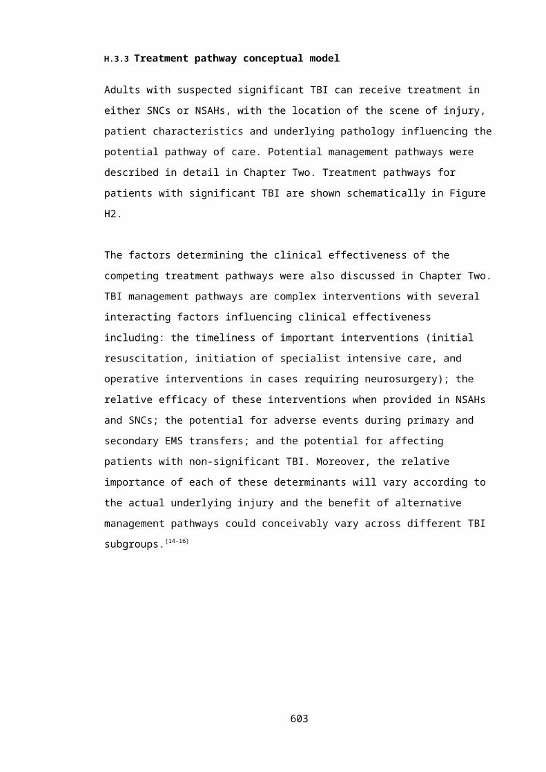
Table J20. Population EVPPI for model parameters under base case assumptions.

Population EVPPI at λ=

Parameter category Relevant model inputs Input type £0 £10,000 £20,000 £30,000 £40,000 £50,000

Population subgroups Mild TBI Proportion £0 £0 £0 £20,744 £0 £0

Acute neurosurgery Proportion £0 £0 £347,385 £5,125,420 £2,945,377 £2,094,278

Head injury requiring critical care Proportion £4,551 £0 £78 £3,395,577 £1,265,634 £573,440

Head injury requiring ward care Proportion £0 £0 £0 £545,185 £0 £0

Major extracranial injury Proportion £0 £7,741 £52,908 £820,492 £0 £0

Relative effectiveness outcomes Acute neurosurgery: NC care Proportional odds ratio £0 £387,949 £5,950,242 £14,341,036 £12,887,713 £12,273,609

(v selective transfer) TBI requiring critical care: Bypass Proportional odds ratio £291,628 £10,053,152 £26,030,71

9

£42,001,498 £47,032,039 £52,453,233

TBI requiring critical care: Routine transfer Proportional odds ratio £770,554 £320,195 £4,918,315 £12,131,555 £9,828,163 £8,565,781

TBI requiring critical care: No transfer Proportional odds ratio £0 £496,243 £407,628 £808,166 £254,226 £212,872

TBI requiring ward care: Bypass Proportional odds ratio £0 £0 £13,981 £622,469 £1,969 £0

Major extracranial injury: Bypass Odds ratio £0 £0 £0 £70,892 £0 £0

Inpatient costs Mild TBI: bypass Incremental cost £0 £0 £0 £2,042,851 £643,573 £553,572

(v selective transfer) Acute neurosurgery: NC care Incremental cost £58,426 £784,175 £3,173,639 £6,698,113 £2,252,809 £525,606

TBI requiring critical care: Bypass Incremental cost £1,465,843 £4,941,885 £9,303,495 £13,673,458 £8,343,931 £4,750,486

603

TBI requiring critical care: Routine transfer Incremental cost £0 £0 £0 £10,129 £0 £0

TBI requiring critical care: No transfer Incremental cost £12,809 £0 £0 £0 £0 £0

TBI requiring ward care: Bypass Incremental cost £0 £0 £0 £709,539 £807 £0

Major extracranial injury: Bypass Incremental cost £0 £0 £45,775 £1,539,086 £12,438 £0

First year post discharge costs GOS severe disability Mean cost £0 £0 £0 £363,534 £0 £0

GOS moderate disability Mean cost £4 £0 £0 £28,111 £0 £0

GOS good recovery Mean cost £0 £0 £15,928 £69,894 £0 £0


Long term costs GOS severe disability Mean cost £839,124 £0 £0 £44,478 £0 £0

GOS moderate disability Mean cost £51 £0 £0 £47,796 £0 £0

GOS good recovery Mean cost £0 £0 £152,706 £1,440,957 £0 £0

EC injury survivors Mean cost £0 £0 £0 £437,994 £0 £0

Utilities GOS severe disability Mean utility £0 £0 £0 £608,237 £0 £0

GOS moderate disability Mean utility £0 £0 £0 £11,555 £0 £0

GOS good recovery Mean utility £0 £0 £0 £787,818 £0 £0

EC injury survivors Mean utility £0 £0 £0 £153,447 £0 £0

Model inputs shaded in grey have large expected values of partial perfect information at NICE willingness to pay thresholds (>£0.5 million).

604

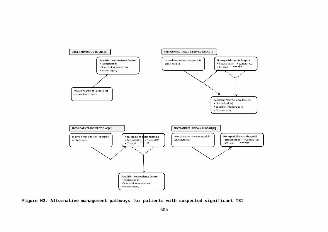
Table J21. Population EVPPI for model parameters, grouped by potential study design, under optimistic assumptions for population that might benefit from

future research.

Optimistic scenario Pessimistic scenario

Population EVPPI (λ=) Population EVPPI (λ=)

£0 £10,000 £20,000 £30,000 £40,000 £50,000 £0 £10,000 £20,000 £30,000 £40,000 £50,000

Patient subgroups £818 £0 £1,714,159 £12,370,18

4

£7,986,953 £6,158,436 £126 £0 £264,005 £1,905,187 £1,230,106 £948,488

TBI utilities £0 £7,443 £558,526 £4,421,639 £1,291,890 £716,864 £0 £1,146 £86,021 £680,996 £198,970 £110,407

Post discharge costs £1,755,95

5

£11,120 £751,228 £5,392,692 £1,024,809 £490,302 £270,44

3

£1,713 £115,700 £830,553 £157,835 £75,514

Bypass: Relative

effectiveness*

£812,668 £21,724,34

5

£54,793,85

6

£87,830,16

9

£99,243,87

9

£111,251,48

5

£125,16

3

£3,345,86

3

£8,439,04

6

£13,527,11

6

£15,284,99

3

£17,134,33

8

Bypass: Inpatient costs* £4,639,27

8

£12,995,63

2

£22,287,92

4

£31,067,48

8

£20,106,63

9

£12,487,650 £714,51

6

£2,001,51

5

£3,432,66

3

£4,784,843 £3,096,713 £1,923,279

*compared with selective transfer

605

J.2.3 Expected net benefit of sampling

The optimal trial design for a future definitive HITSNS study, comparing prehospital triage and

bypass with selective secondary transfer, was sensitive to varying assumptions on trial

characteristics, disease incidence, technology lifespan, and patient recruitment limits. Taking

an optimistic viewpoint on these factors, the most cost-effective trial design at NICE thresholds

would be achieved with a trial of 2,052 patients recruited from 10 ambulance services, in 480

ambulance stations, and lasting a total of 2 years. Taking pessimistic assumptions resulted in

much lower ENBS, but a future trial was still shown to be cost-effective, with the most

favourable trial recruiting 636 patients (5 ambulance services, 140 clusters, 5 years in total) at

both λ=£20,000 and λ=£30,000. The study characteristics for a definitive trial envisaged in the

original HITSNS pilot study protocol resulted in a very similar optimum design of 624 patients

(4 ambulance services, 120 clusters, 4 years in total). Interestingly, careful enumeration of

fixed and variable trial expenditure, informed by HITSNS pilot study funding, gave very similar

trial costs to the base case estimate using a marginal per patient estimate (data not shown).

Methodology and assumptions for sensitivity analyses examining ENBS and properties of

optimal trials in different scenarios were detailed in Chapter Eight. Results from these analyses

are summarised in Table J22, and presented in detail in Tables J23 to J25, and Figures J2 to J7.

Table J22. Summary of optimal trial designs under different assumptions for recruitment and

trial characteristics.

Scenario* Total sample size

Number of clusters

Number of ambulance services

Trial duration (years)

Base case 1,040 347 8 3

Optimistic scenario 2,052 480 10 2

Pessimistic scenario 636 140 5 5

Planned definitive HITSNS trial

624 120 4 4

*Assumptions of different scenarios were detailed in Chapter 8.

606

Table J23. Expected net benefit of sampling and study characteristics of definitive HITSNS trial with differing sample sizes under optimistic assumptions.

λ=£20,000 λ=£30,000

Sample

size

Number

of

clusters

Number of

ambulance

services

Total trial

duration

(years)*

Trial costs Individual EVSI Population EVSI ENBS Individual EVSI Population

EVSI

ENBS

0 0 0 0 £0 £0 £0 £0 £0 £0 £0

103 29 1 2 £51,300 £240 £7,811,733 £7,760,433 £644 £20,966,309 £20,915,009

205 57 1 2 £102,600 £420 £13,660,193 £13,557,593 £915 £29,776,163 £29,673,563

257 71 1 2 £128,250 £535 £17,413,016 £17,284,766 £990 £32,221,950 £32,093,700

513 143 2 2 £256,500 £741 £24,130,840 £23,874,340 £1,310 £42,638,364 £42,381,864

616 171 3 2 £307,800 £837 £27,252,741 £26,944,941 £1,338 £43,542,955 £43,235,155

821 228 4 2 £410,400 £882 £28,691,377 £28,280,977 £1,510 £49,134,396 £48,723,996

1026 285 5 2 £513,000 £919 £29,922,343 £29,409,343 £1,583 £51,514,712 £51,001,712

1231 342 6 2 £615,600 £976 £31,753,108 £31,137,508 £1,694 £55,125,459 £54,509,859

1642 456 8 2 £820,800 £1,032 £33,594,604 £32,773,804 £1,791 £58,271,886 £57,451,086

2052 480 10 2 £1,026,000 £1,104 £35,924,767 £34,898,767 £1,869 £60,825,699 £59,799,699

3078 480 10 3 £1,539,000 £1,174 £34,465,433 £32,926,433 £1,975 £57,983,380 £56,444,380

4104 480 10 3 £2,052,000 £1,228 £36,051,502 £33,999,502 £2,001 £58,749,093 £56,697,093

5130 480 10 4 £2,565,000 £1,264 £33,144,144 £30,579,144 £2,067 £54,194,420 £51,629,420

8208 480 10 5 £4,104,000 £1,315 £30,432,323 £26,328,323 £2,130 £49,280,849 £45,176,849

10260 480 10 6 £5,130,000 £1,337 £26,859,074 £21,729,074 £2,151 £43,205,532 £38,075,532

*Including analysis, reporting, dissemination and implementation.

Optimal trial highlighted in grey.

607

Figure J2. Expected net benefit of sampling for a definitive HITSNS cluster randomised trial at

λ=£20,000 (optimistic assumptions).


λ=£30,000 (optimistic assumptions).

608

Table J24. Expected net benefit of sampling and study characteristics of definitive HITSNS trial with differing sample sizes under pessimistic assumptions.

λ=£20,000 λ=£30,000

Sample

size

Number

of

clusters

Number of

ambulance

services

Total trial

duration

(years)*


EVSI

ENBS

0 0 0 0 £0 £0 £0 £0 £0 £0 £0

106 42 2 4 £212,000 £240 £638,166 £426,166 £644 £1,712,807 £1,500,807

212 85 3 4 £424,000 £420 £1,115,946 £691,946 £915 £2,432,513 £2,008,513

265 106 4 4 £530,000 £535 £1,422,527 £892,527 £990 £2,632,318 £2,102,318

530 140 5 5 £1,060,000 £741 £1,434,622 £374,622 £1,310 £2,534,928 £1,474,928

636 140 5 5 £1,272,000 £837 £1,620,225 £348,225 £1,338 £2,588,707 £1,316,707

848 140 5 6 £1,696,000 £882 £1,103,736 -£592,264 £1,510 £1,890,164 £194,164

1060 140 5 7 £2,120,000 £919 £558,782 -£1,561,218 £1,583 £962,006 -£1,157,994

1272 140 5 7 £2,544,000 £976 £592,970 -£1,951,030 £1,694 £1,029,435 -£1,514,565

1696 140 5 8 £3,392,000 £1,032 £0 -£3,392,000 £1,791 £0 -£3,392,000

2120 140 5 10 £4,240,000 £1,104 £0 -£4,240,000 £1,869 £0 -£4,240,000

3180 140 5 13 £6,360,000 £1,174 £0 -£6,360,000 £1,975 £0 -£6,360,000

4240 140 5 16 £8,480,000 £1,228 £0 -£8,480,000 £2,001 £0 -£8,480,000

5300 140 5 19 £10,600,000 £1,264 £0 -£10,600,000 £2,067 £0 -£10,600,000

8480 140 5 28 £16,960,000 £1,315 £0 -£16,960,000 £2,130 £0 -£16,960,000

10600 140 5 34 £21,200,000 £1,337 £0 -£21,200,000 £2,151 £0 -£21,200,000



609


λ=£20,000 (pessimistic assumptions).


λ=£30,000 (pessimistic assumptions).

610

Table J25. Expected net benefit of sampling and study characteristics of definitive HITSNS trial with differing sample sizes under assumptions consistent with

originally envisaged definitive HITSNS trial.

λ=£20,000 λ=£30,000

Sample

size

Number

of

clusters

Number of

ambulance

services

Total trial

duration

(years)*


EVSI

ENBS

0 0 0 0 £0 £0 £0 £0 £0 £0 £0

104 35 1 3 £707,792 £240 £3,134,385 £2,426,592 £644 £8,412,535 £7,704,743

208 69 2 3 £897,835 £420 £5,481,025 £4,583,190 £915 £11,947,407 £11,049,573

260 87 3 3 £978,146 £535 £6,986,810 £6,008,664 £990 £12,928,756 £11,950,610

520 120 4 4 £1,454,508 £741 £8,152,339 £6,697,831 £1,310 £14,404,903 £12,950,395

624 120 4 4 £1,468,028 £837 £9,207,039 £7,739,011 £1,338 £14,710,509 £13,242,481

832 120 4 5 £1,775,818 £882 £7,935,501 £6,159,683 £1,510 £13,589,659 £11,813,841

1040 120 4 5 £1,802,858 £919 £8,275,963 £6,473,105 £1,583 £14,248,010 £12,445,152

1248 120 4 6 £2,110,648 £976 £6,902,976 £4,792,328 £1,694 £11,984,014 £9,873,366

1664 120 4 7 £2,445,478 £1,032 £5,382,213 £2,936,735 £1,791 £9,335,775 £6,890,297

2080 120 4 8 £2,780,308 £1,104 £3,770,655 £990,347 £1,869 £6,384,251 £3,603,943

3120 120 4 11 £3,757,758 £1,174 £0 -£3,757,758 £1,975 £0 -£3,757,758

4160 120 4 14 £4,735,208 £1,228 £0 -£4,735,208 £2,001 £0 -£4,735,208

5200 120 4 17 £5,712,658 £1,264 £0 -£5,712,658 £2,067 £0 -£5,712,658

8320 120 4 26 £8,645,008 £1,315 £0 -£8,645,008 £2,130 £0 -£8,645,008

10400 120 4 31 £10,319,158 £1,337 £0 -£10,319,158 £2,151 £0 -£10,319,158



611


λ=£20,000 (originally planned definitive HITSNS trial assumptions).


λ=£30,000 (originally planned definitive HITSNS trial assumptions).

612

J.3 REFERENCES


2. Taussky P, Widmer HR, Takala J, Fandino J: Outcome after acute traumatic subdural and epidural haematoma in Switzerland: a single-centre experience. Swiss medical weekly 2008, 138(19-20):281-285.

3. Fuller G PH, Yeoman P. : The Nottingham Head Injury Register: a Survey of 1,276 Adult cases of Moderate and Severe Traumatic Brain Injury in a British Neurosurgery Centre. . Journal of Intensive Care Society 2011, 12(1):1-7.




7. McMillan TM, Teasdale GM, Stewart E: Disability in young people and adults after head injury: 12-14 year follow-up of a prospective cohort. Journal of neurology, neurosurgery, and psychiatry 2012, 83(11):1086-1091.

8. Whitnall L, McMillan TM, Murray GD, Teasdale GM: Disability in young people and adults after head injury: 5-7 year follow up of a prospective cohort study. J Neurol Neurosurg Psychiatry 2006, 77(5):640-645.

613