appendix i raw data - duke university · a2 table a1. canal sampling station raw data. station...
TRANSCRIPT
A1
APPENDIX I
RAW DATA
A2
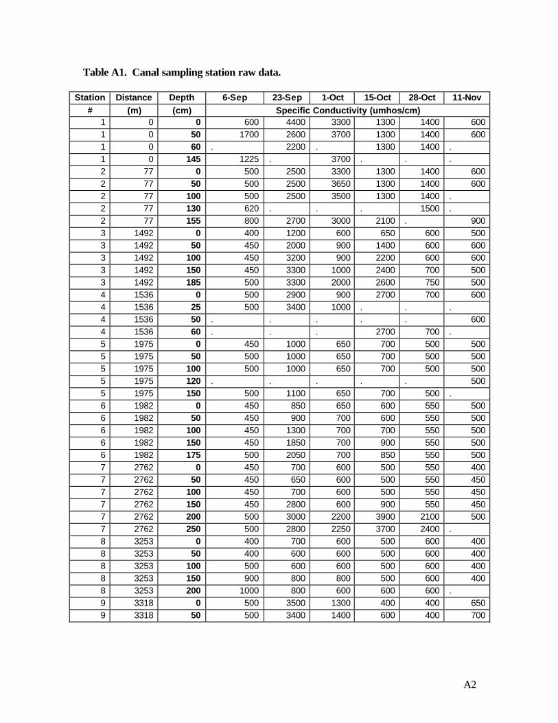
Table A1. Canal sampling station raw data.
Station Distance Depth 6-Sep 23-Sep 1-Oct 15-Oct 28-Oct 11-Nov # (m) (cm) Specific Conductivity (umhos/cm)
1 0 0 600 4400 3300 1300 1400 600 1 0 50 1700 2600 3700 1300 1400 600 1 0 60 . 2200 . 1300 1400 . 1 0 145 1225 . 3700 . . . 2 77 0 500 2500 3300 1300 1400 600 2 77 50 500 2500 3650 1300 1400 600 2 77 100 500 2500 3500 1300 1400 . 2 77 130 620 . . . 1500 . 2 77 155 800 2700 3000 2100 . 900 3 1492 0 400 1200 600 650 600 500 3 1492 50 450 2000 900 1400 600 600 3 1492 100 450 3200 900 2200 600 600 3 1492 150 450 3300 1000 2400 700 500 3 1492 185 500 3300 2000 2600 750 500 4 1536 0 500 2900 900 2700 700 600 4 1536 25 500 3400 1000 . . . 4 1536 50 . . . . . 600 4 1536 60 . . . 2700 700 . 5 1975 0 450 1000 650 700 500 500 5 1975 50 500 1000 650 700 500 500 5 1975 100 500 1000 650 700 500 500 5 1975 120 . . . . . 500 5 1975 150 500 1100 650 700 500 . 6 1982 0 450 850 650 600 550 500 6 1982 50 450 900 700 600 550 500 6 1982 100 450 1300 700 700 550 500 6 1982 150 450 1850 700 900 550 500 6 1982 175 500 2050 700 850 550 500 7 2762 0 450 700 600 500 550 400 7 2762 50 450 650 600 500 550 450 7 2762 100 450 700 600 500 550 450 7 2762 150 450 2800 600 900 550 450 7 2762 200 500 3000 2200 3900 2100 500 7 2762 250 500 2800 2250 3700 2400 . 8 3253 0 400 700 600 500 600 400 8 3253 50 400 600 600 500 600 400 8 3253 100 500 600 600 500 600 400 8 3253 150 900 800 800 500 600 400 8 3253 200 1000 800 600 600 600 . 9 3318 0 500 3500 1300 400 400 650 9 3318 50 500 3400 1400 600 400 700

A3
Table A1 (continued). Canal sampling station raw data.
Station Distance Depth 6-Sep 23-Sep 1-Oct 15-Oct 28-Oct 11-Nov # (m) (cm) Specific Conductivity (umhos/cm)
9 3318 80 500 3400 1400 1200 600 700 10 4641 50 600 1000 1000 600 500 500 10 4641 100 625 900 900 600 500 500 10 4641 150 950 900 900 600 500 500 10 4641 200 1150 1200 900 900 500 500
Table A2. Monitoring well specific conductivity and water table raw data.
Transect Well Distance
6-Sep 23-Sep 1-Oct 15-Oct 28-Oct 11-Nov
(m) Specific Conductivity (umhos/cm) Spur Rd 5 1225 1200 1300 1100 1300 1100 Spur Rd 15 1200 800 800 2000 700 900 Spur Rd 30 825 1000 900 600 750 700 USGS 5 700 550 600 900 700 600 USGS 15 450 450 600 600 400 400 USGS 30 400 400 500 500 400 350 Mouth 5 2800 4600 3000 3500 3100 2300 Mouth 15 2200 4950 3300 3900 2350 2200 Mouth 30 3500 4700 2800 4350 2700 2600 Shore 5 . . . 7500 6500 5000 Shore 15 . . . 3600 2700 2800 Shore 30 6000 4400 3800 3500 3000 2700 Depth to Water Table (cm) Spur Rd 5 -2.8 -5.5 0 -15.5 -16 -6 Spur Rd 15 -16 -9 -3 -10 -12.5 -10 Spur Rd 30 1.2 -0.5 0 0 -1.5 0 USGS 5 -0.3 -5 -1 -11 -18 -7.5 USGS 15 2.8 1.5 1 -5.5 -11 -1 USGS 30 2.3 0.5 0 -8.5 -11 -3 Mouth 5 9.3 0 -1 -0.5 -5 -1.5 Mouth 15 112.2 6.5 8 -1 -4 4.75 Mouth 30 124.2 9 6 -2.5 -5 2.5 Shore 5 . . . 28 22 37 Shore 15 . . . 13 13 26 Shore 30 77 9 20 -2 -1.5 27
A4
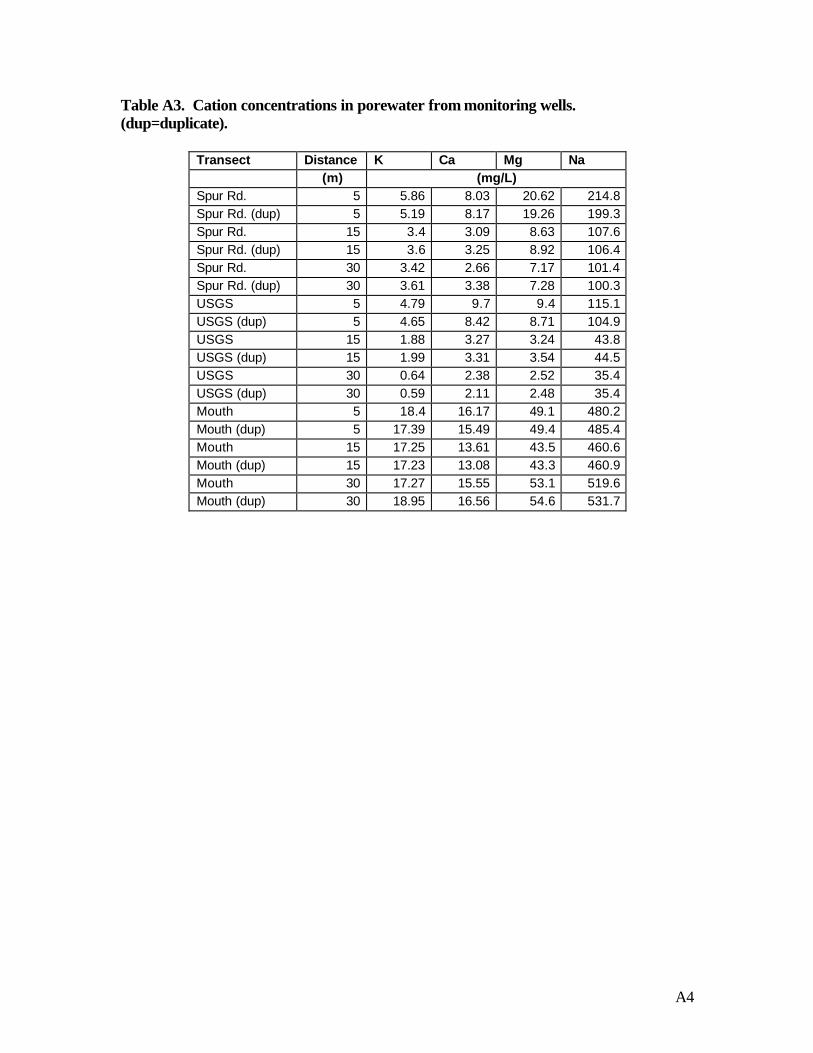
Table A3. Cation concentrations in porewater from monitoring wells. (dup=duplicate).
Transect Distance K Ca Mg Na (m) (mg/L) Spur Rd. 5 5.86 8.03 20.62 214.8 Spur Rd. (dup) 5 5.19 8.17 19.26 199.3 Spur Rd. 15 3.4 3.09 8.63 107.6 Spur Rd. (dup) 15 3.6 3.25 8.92 106.4 Spur Rd. 30 3.42 2.66 7.17 101.4 Spur Rd. (dup) 30 3.61 3.38 7.28 100.3 USGS 5 4.79 9.7 9.4 115.1 USGS (dup) 5 4.65 8.42 8.71 104.9 USGS 15 1.88 3.27 3.24 43.8 USGS (dup) 15 1.99 3.31 3.54 44.5 USGS 30 0.64 2.38 2.52 35.4 USGS (dup) 30 0.59 2.11 2.48 35.4 Mouth 5 18.4 16.17 49.1 480.2 Mouth (dup) 5 17.39 15.49 49.4 485.4 Mouth 15 17.25 13.61 43.5 460.6 Mouth (dup) 15 17.23 13.08 43.3 460.9 Mouth 30 17.27 15.55 53.1 519.6 Mouth (dup) 30 18.95 16.56 54.6 531.7

A5
Table A4. Soil parameters at each monitoring well. Transect Distance Depth
from surface
Bulk Density
Soil Organic Matter
Carbon Nitrogen C:N
(cm) g/cm3 % % % Spur Rd. 5 11 to 21 0.0798 98.40 52.01 1.95 26.62233 Spur Rd. 5 21 to 31 0.1936 96.13 53.27 2.18 24.44544 Spur Rd. 15 7 to 17 0.0461 99.69 55.47 2.30 24.16688 Spur Rd. 15 17 to 27 0.0975 99.35 54.24 1.84 29.46196 Spur Rd. 30 2 to 12 0.0441 99.85 56.44 1.95 28.93169 Spur Rd. 30 12 to 22 0.0630 99.79 50.91 1.88 27.05682 USGS 5 12 to 22 0.1150 97.70 52.35 2.06 25.42821 USGS 5 22 to 32 0.0911 98.18 47.60 1.70 28.04907 USGS 15 5 to 15 0.0963 99.36 47.67 1.78 26.79967 USGS 15 15 to 25 0.1015 99.32 46.92 1.53 30.6218 USGS 30 1 to 11 0.0999 99.67 49.04 2.17 22.55359 USGS 30 11 to 21 0.0882 99.71 30.58 0.91 33.77504 Mouth 5 26 to 36 0.2041 95.92 9.71 0.45 21.39554 Mouth 5 36 to 46 0.1926 96.15 20.67 0.72 28.52464 Mouth 15 37 to 47 0.5401 96.40 21.94 0.86 25.48531 Mouth 15 47 to 57 0.6570 95.62 4.48 0.24 18.74899 Mouth 30 34 to 44 0.2900 99.03 12.11 0.65 18.65287 Mouth 30 44 to 54 1.0156 96.61 7.58 0.45 16.88517 Shore 5 0 to 4.5 0.2743 94.51 31.58 1.30 24.33788 Shore 15 0 to 10 0.4164 97.22 8.53 0.49 17.37279 Shore 15 10 to 20 0.2960 98.03 15.10 0.70 21.69563 Shore 30 4 to 14 0.2718 99.09 7.39 0.37 19.9244 Shore 30 14 to 24 0.5560 98.15 7.68 0.39 19.66316

A6
APPENDIX II
SUMMARY STATISTICS

A7
Table B1. Mean conductivity ± 1SE at each monitoring well. Values with the same letters are not significantly different (p>0.05) from each other.
Transect Distance from edge
(m)
Average Specific Conductivity
(umhos/cm)
N
Spur Rd.a 5 1204.17 ± 36.75 6
15 1066.67 ± 199.44 6
30 795.83 ± 58.6 6
USGSb 5 675 ± 51.23 6
15 483.3 ± 38 6
30 425 ± 25 6
Mouthc 5 3216.67 ± 319.8 6
15 3150 ± 457.16 6
30 3441.67 ± 368.88 6
Shored 5 6333.33 ± 726.48 3
15 3033.33 ± 284.8 3
30 3900 ± 485.8 3

A8
Table B2. Mean potassium concentrations ± 1SE at each monitoring well. Values with the same letters are not significantly different (p>0.05) from each other.
Transect Distance from edge
(m)
Cation Concentration
(mg/L)
N
Spur Rd. 5a 5.525 ± 0.335 2
15b 3.5 ± 0.1 2
30b 3.515 ± 0.095 2
USGS 5a 4.72 ± 0.07 2
15c 1.935 ± 0.055 2
30d 0.615 ± 0.025 2
Mouth 5e 17.895 ± 0.505 2
15e 17.24 ± 0.01 2
30e 18.11 ± 0.84 2
Table B3. Mean calcium concentrations ± 1SE at each monitoring well. Values with the same letters are not significantly different (p>0.05) from each other.
Transect Distance from edge
(m)
Cation Concentration
(mg/L)
N
Spur Rd. 5a 8.1 ± 0.07 2
15b 3.17 ± 0.08 2
30b 3.02 ± 0.36 2
USGS 5a 9.06 ± 0.64 2
15b 3.29 ± 0.02 2
30bc 2.24 ± 0.135 2
Mouth 5d 15.83 ± 0.34 2
15d 13.345 ± 0.265 2
30d 16.055 ± 0.505 2

A9
Table B4. Mean magnesium concentrations ± 1SE at each monitoring well. Values with the same letters are not significantly different (p>0.05) from each other.
Transect Distance from edge
(m)
Cation Concentration
(mg/L)
N
Spur Rd. 5a 19.94 ± 0.68 2
15b 8.775 ± 0.145 2
30c 7.225 ± 0.055 2
USGS 5b 9.055 ± 0.345 2
15d 3.39 ± 0.15 2
30e 2.5 ± 0.02 2
Mouth 5f 49.25 ± 0.15 2
15fg 43.4 ± 0.1 2
30f 53.85 ± 0.75 2
Table B5. Mean sodium concentrations ± 1SE at each monitoring well. Values with the same letters are not significantly different (p>0.05) from each other.
Transect Distance from edge
(m)
Cation Concentration
(mg/L)
N
Spur Rd. 5a 207.05 ± 7.75 2
15b 107.0 ± 0.6 2
30b 100.85 ± 0.55 2
USGS 5b 110.0 ± 5.1 2
15c 44.15 ± 0.35 2
30d 35.4 ± 0 2
Mouth 5e 482.8 ± 2.6 2
15ef 460.75 ± 0.15 2
30e 525.65 ± 6.05 2

A10
Table B6. Mean soil bulk density ± 1SE at each monitoring well. Values with the same letters are not significantly different (p>0.05) from each other.
Transect Distance from edge
(m)
Bulk density
(g/cm3)
N
Spur Rd. 5a 0.1367 ± 0.0569 2
15a 0.0718 ± 0.0257 2
30a 0.05355 ± 0.009 2
USGS 5a 0.10305 ± 0.01195 2
15a 0.0989 ± 0.0026 2
30a 0.09405 ± 0.0059 2
Mouth 5a 0.19835 ± 0.0057 2
15ab 0.59855 ± 0.05845 2
30b 0.7528 ± 0.2628 2
Shore 5ab 0.3525 1
15ab 0.3562 ± 0.0602 2
30ab 0.4139 ± 0.1421 2

A11
Table B7. Mean percent soil organic matter ± 1SE at each monitoring well. Values with the same letters are not significantly different (p>0.05) from each other.
Transect Distance from edge
(m)
Soil Organic Matter
(%)
N
Spur Rd. 5a 60.405 ± 1.785 2
15b 92.74 ± 3.16 2
30b 93.72 ± 1.42 2
USGS 5b 94.24 ± 0.87 2
15b 95.0 ± 0.33 2
30b 95.035 ± 1.945 2
Mouth 5a 42.67 ± 1.82 2
15c 17.745 ± 2.405 2
30c 17.705 ± 7.935 2
Shore 5ac 21.32 1
15ac 27.745 ± 7.765 2
30ac 24.425 ± 7.545 2

A12
Table B8. Mean carbon:nitrogen ± 1SE at each monitoring well. C:N ratios are not significantly different (p>0.05) from each other.
Transect Distance from edge
(m)
C:N
N
Spur Rd. 5a 29.06 ± 4.72 2
15a 26.585 ± 4.035 2
30a 27.425 ± 0.625 2
USGS 5a 26.245 ± 0.815 2
15a 29.195 ± 0.265 2
30a 25.535 ± 1.08 2
Mouth 5a 27.005 ± 1.515 2
15a 20.66 ± 0.74 2
30a 18.7 ± 0.05 2
Shore 5a 19.28 1
15a 19.535 ± 2.165 2
30a 17.975 ± 1.085 2

A13
APPENDIX III
SAS CODE

A14
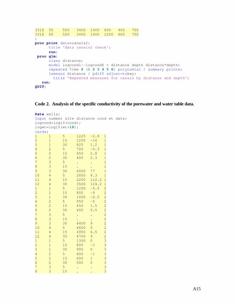
Code 1. Analysis of surface water from canal sampling stations. Data canals2; Input distance depth cond1 cond2 cond3 cond4 cond5 cond6; logcond1=log10(cond1); logcond2=log10(cond2); logcond3=log10(cond3); logcond4=log10(cond4); logcond5=log10(cond5); logcond6=log10(cond6); cards; 77 0 500 2500 3300 1300 1400 600 77 50 500 2500 3650 1300 1400 600 77 100 500 2500 3500 1300 1400 . 77 130 620 . . . 1500 . 77 155 800 2700 3000 2100 . 900 0 0 600 4400 3300 1300 1400 600 0 50 1700 2600 3700 1300 1400 600 0 60 . 2200 . 1300 1400 . 0 145 1225 . 3700 . . . 1536 0 500 2900 900 2700 700 600 1536 25 500 3400 1000 . . . 1536 50 . . . . . 600 1536 60 . . . 2700 700 . 1492 0 400 1200 600 650 600 500 1492 50 450 2000 900 1400 600 600 1492 100 450 3200 900 2200 600 600 1492 150 450 3300 1000 2400 700 500 1492 185 500 3300 2000 2600 750 500 1975 0 450 1000 650 700 500 500 1975 50 500 1000 650 700 500 500 1975 100 500 1000 650 700 500 500 1975 120 . . . . . 500 1975 150 500 1100 650 700 500 . 1982 0 450 850 650 600 550 500 1982 50 450 900 700 600 550 500 1982 100 450 1300 700 700 550 500 1982 150 450 1850 700 900 550 500 1982 175 500 2050 700 850 550 500 4641 0 625 . 1000 600 500 500 4641 50 600 1000 1000 600 500 500 4641 100 625 900 900 600 500 500 4641 150 950 900 900 600 500 500 4641 200 1150 1200 900 900 500 500 3253 0 400 700 600 500 600 400 3253 50 400 600 600 500 600 400 3253 100 500 600 600 500 600 400 3253 150 900 800 800 500 600 400 3253 200 1000 800 600 600 600 . 2762 0 450 700 600 500 550 400 2762 50 450 650 600 500 550 450 2762 100 450 700 600 500 550 450 2762 150 450 2800 600 900 550 450 2762 200 500 3000 2200 3900 2100 500 2762 250 500 2800 2250 3700 2400 . 3318 0 500 3500 1300 400 400 650
A15
3318 50 500 3400 1400 600 400 700 3318 80 500 3400 1400 1200 600 700 ; proc print data=canals2; title "data canals2 check"; run; proc glm; class distance; model logcond1--logcond6 = distance depth distance*depth; repeated Time 6 (1 2 3 4 5 6) polynomial / summary printe; lsmeans distance / pdiff adjust=tukey; title "Repeated measures for canals by distance and depth"; run; QUIT;
Code 2. Analysis of the specific conductivity of the porewater and water table data. Data wells; Input number site distance cond wt date; logcond=log10(cond); logwt=log10(wt+18); cards; 1 1 5 1225 -2.8 1 2 1 15 1200 -16 1 3 1 30 825 1.2 1 4 2 5 700 -0.3 1 5 2 15 450 2.8 1 6 2 30 400 2.3 1 7 3 5 . . 1 8 3 15 . . 1 9 3 30 6000 77 1 10 4 5 2800 9.3 1 11 4 15 2200 112.2 1 12 4 30 3500 124.2 1 1 1 5 1200 -5.5 2 2 1 15 800 -9 2 3 1 30 1000 -0.5 2 4 2 5 550 -5 2 5 2 15 450 1.5 2 6 2 30 400 0.5 2 7 3 5 . . 2 8 3 15 . . 2 9 3 30 4400 9 2 10 4 5 4600 0 2 11 4 15 4950 6.5 2 12 4 30 4700 9 2 1 1 5 1300 0 3 2 1 15 800 -3 3 3 1 30 900 0 3 4 2 5 600 -1 3 5 2 15 600 1 3 6 2 30 500 0 3 7 3 5 . . 3 8 3 15 . . 3
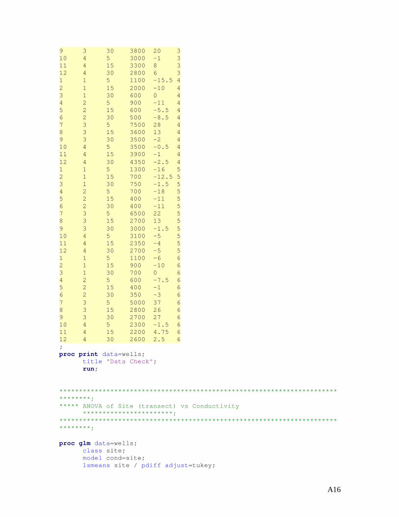
A16
9 3 30 3800 20 3 10 4 5 3000 -1 3 11 4 15 3300 8 3 12 4 30 2800 6 3 1 1 5 1100 -15.5 4 2 1 15 2000 -10 4 3 1 30 600 0 4 4 2 5 900 -11 4 5 2 15 600 -5.5 4 6 2 30 500 -8.5 4 7 3 5 7500 28 4 8 3 15 3600 13 4 9 3 30 3500 -2 4 10 4 5 3500 -0.5 4 11 4 15 3900 -1 4 12 4 30 4350 -2.5 4 1 1 5 1300 -16 5 2 1 15 700 -12.5 5 3 1 30 750 -1.5 5 4 2 5 700 -18 5 5 2 15 400 -11 5 6 2 30 400 -11 5 7 3 5 6500 22 5 8 3 15 2700 13 5 9 3 30 3000 -1.5 5 10 4 5 3100 -5 5 11 4 15 2350 -4 5 12 4 30 2700 -5 5 1 1 5 1100 -6 6 2 1 15 900 -10 6 3 1 30 700 0 6 4 2 5 600 -7.5 6 5 2 15 400 -1 6 6 2 30 350 -3 6 7 3 5 5000 37 6 8 3 15 2800 26 6 9 3 30 2700 27 6 10 4 5 2300 -1.5 6 11 4 15 2200 4.75 6 12 4 30 2600 2.5 6 ; proc print data=wells; title "Data Check"; run; *******************************************************************************; ***** ANOVA of Site (transect) vs Conductivity ***********************; *******************************************************************************; proc glm data=wells; class site; model cond=site; lsmeans site / pdiff adjust=tukey;

A17
output out=one predicted=p residual=r; title "ANOVA of Conductivity Against Transect"; run; proc univariate data=one normal plot; var r; title5 "Univariate Analysis of Residuals for Normality"; run; proc plot data=one; plot r*p; title5 "Plot of Predicted vs Residuals for HOV Analysis"; run; *******************************************************************************; ***** ANCOVA of site (transect) vs Conductivity: Log-Transformed Data ***; *******************************************************************************; proc glm data=wells; class site; model logcond=site; lsmeans site / pdiff adjust=tukey; output out=two predicted=p residual=r; title "ANOVA of Conductivity Against site (transect) logcond"; run; proc univariate data=two normal plot; var r; title5 "Univariate Analysis of Residuals for Normality - logcond"; run; proc plot data=two; plot r*p; title5 "Plot of Predicted vs Residuals for HOV Analysis - logcond"; run; proc means data=wells N MEAN STDERR ; var cond; class site; title5 "Means Calculations"; run; *****************************************************************************************; ***** ANCOVA of Transect and distance vs Conductivity: Log-Transformed Data *****; *****************************************************************************************; proc glm data=wells; class site;

A18
model logcond=site distance / solution; lsmeans site / pdiff adjust=tukey; output out=three predicted=p residual=r; title "ANCOVA of Conductivity Against transect and distance (logcond)"; run; proc univariate data=three normal plot; var r; title5 "Univariate Analysis of Residuals for Normality"; run; proc plot data=three; plot r*p; title5 "Plot of Predicted vs Residuals for HOV Analysis"; run; proc means data=wells N MEAN STDERR ; var cond; class site; title5 "Means Calculations Site"; run; proc means data=wells N MEAN STDERR ; var cond; class distance; title "Means Calculations Distance"; run; proc means data=wells N MEAN STDERR ; var cond; class site distance; title "Means Calculations Site*Distance"; run; proc glm data=wells; class site; model logcond=site distance site*distance; lsmeans site / pdiff adjust=tukey; lsmeans distance / pdiff adjust=tukey; lsmeans site*distance / pdiff adjust=tukey; title "ANOVA Conductivity against site distance and site*distance"; run; proc glm data=wells; class site date; model logcond=site distance site*distance date site*date date*site*distance; title "ANOVA site distance and date with interaction"; run; proc glm data=wells; class date; model logcond=date; title "ANOVA of conductivity against date"; run;

A19
*****************************************************************************************; ***** Water Table vs Conductivity: Regression and ANOVA *****************************; *****************************************************************************************; proc corr data=wells; var logcond wt; title "correlation between conductivity and water table"; run; proc glm data=wells; model logcond=wt; Title "Regression of logcond and wt"; run; proc glm data=wells; model logcond=wt wt*wt; Title "Polynomial water table regression"; run; proc plot data=wells; plot logcond*wt; run; proc reg data=wells; model logcond=wt / all influence; Title "Regression of Conductivity against Water Table"; run; QUIT; Code 3. Analysis of the cation concentration data from the porewater. Data cations; Input site distance cond wt k ca mg na; logcond=log10(cond); logwt=log10(wt+18); logk=log10(k); logca=log10(ca); logmg=log10(mg); logna=log10(na); cards; 1 5 1100 -6 5.86 8.03 20.62 214.8 1 5 1100 -6 5.19 8.17 19.26 199.3 1 15 900 -10 3.4 3.09 8.63 107.6 1 15 900 -10 3.6 3.25 8.92 106.4 1 30 700 0 3.42 2.66 7.17 101.4 1 30 700 0 3.61 3.38 7.28 100.3 2 5 600 -7.5 4.79 9.7 9.4 115.1 2 5 600 -7.5 4.65 8.42 8.71 104.9 2 15 400 -1 1.88 3.27 3.24 43.8 2 15 400 -1 1.99 3.31 3.54 44.5 2 30 350 -3 0.64 2.38 2.52 35.4 2 30 350 -3 0.59 2.11 2.48 35.4 3 5 2300 -1.5 18.4 16.17 49.1 480.2 3 5 2300 -1.5 17.39 15.49 49.4 485.4
A20
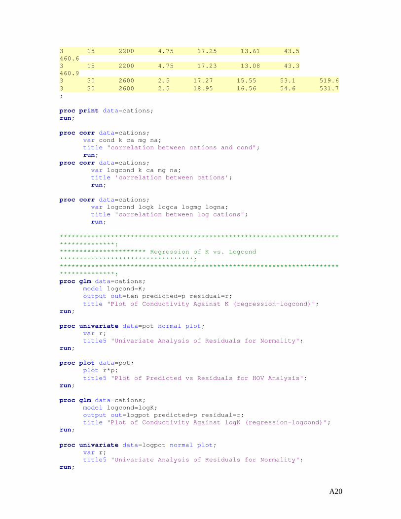
3 15 2200 4.75 17.25 13.61 43.5 460.6 3 15 2200 4.75 17.23 13.08 43.3 460.9 3 30 2600 2.5 17.27 15.55 53.1 519.6 3 30 2600 2.5 18.95 16.56 54.6 531.7 ; proc print data=cations; run; proc corr data=cations; var cond k ca mg na; title "correlation between cations and cond"; run; proc corr data=cations; var logcond k ca mg na; title 'correlation between cations'; run; proc corr data=cations; var logcond logk logca logmg logna; title "correlation between log cations"; run; *************************************************************************************; ********************** Regression of K vs. Logcond **********************************; *************************************************************************************; proc glm data=cations; model logcond=K; output out=ten predicted=p residual=r; title "Plot of Conductivity Against K (regression-logcond)"; run; proc univariate data=pot normal plot; var r; title5 "Univariate Analysis of Residuals for Normality"; run; proc plot data=pot; plot r*p; title5 "Plot of Predicted vs Residuals for HOV Analysis"; run; proc glm data=cations; model logcond=logK; output out=logpot predicted=p residual=r; title "Plot of Conductivity Against logK (regression-logcond)"; run; proc univariate data=logpot normal plot; var r; title5 "Univariate Analysis of Residuals for Normality"; run;
A21
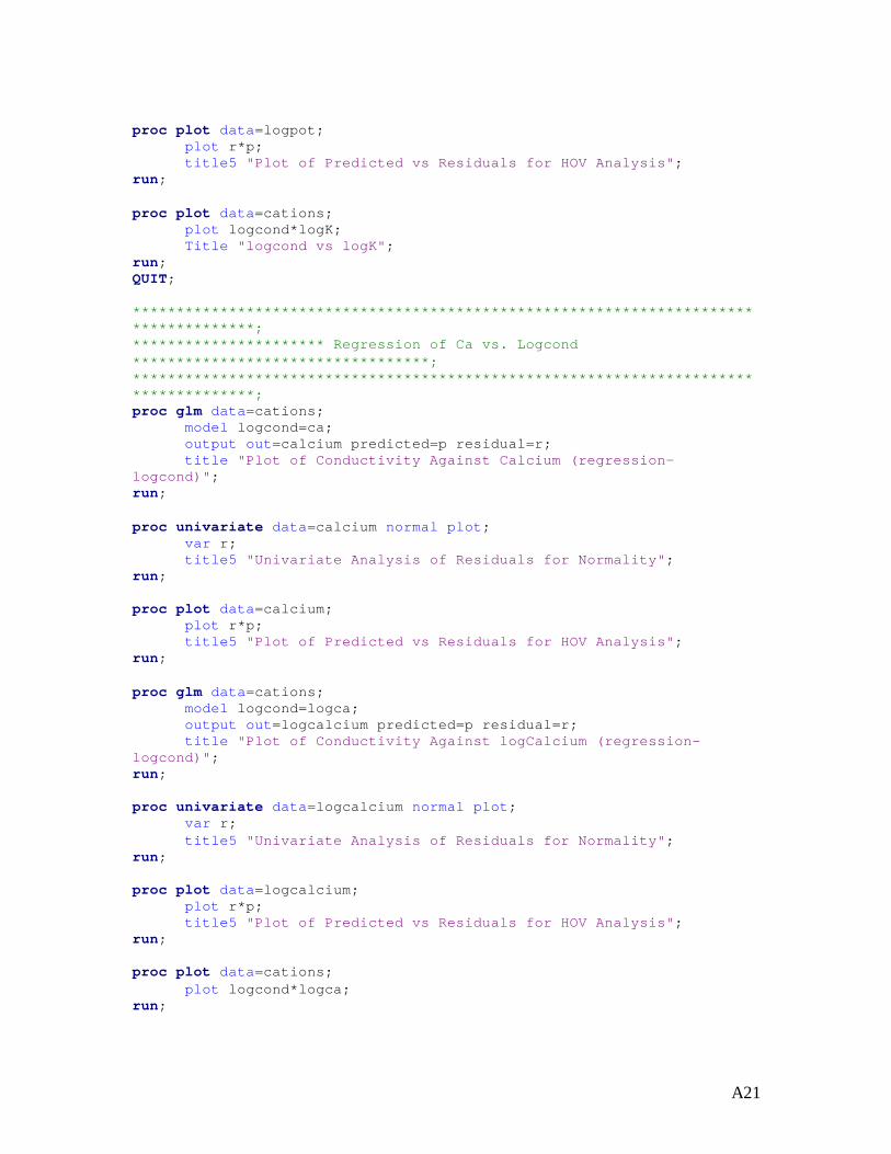
proc plot data=logpot; plot r*p; title5 "Plot of Predicted vs Residuals for HOV Analysis"; run; proc plot data=cations; plot logcond*logK; Title "logcond vs logK"; run; QUIT; *************************************************************************************; ********************** Regression of Ca vs. Logcond **********************************; *************************************************************************************; proc glm data=cations; model logcond=ca; output out=calcium predicted=p residual=r; title "Plot of Conductivity Against Calcium (regression-logcond)"; run; proc univariate data=calcium normal plot; var r; title5 "Univariate Analysis of Residuals for Normality"; run; proc plot data=calcium; plot r*p; title5 "Plot of Predicted vs Residuals for HOV Analysis"; run; proc glm data=cations; model logcond=logca; output out=logcalcium predicted=p residual=r; title "Plot of Conductivity Against logCalcium (regression-logcond)"; run; proc univariate data=logcalcium normal plot; var r; title5 "Univariate Analysis of Residuals for Normality"; run; proc plot data=logcalcium; plot r*p; title5 "Plot of Predicted vs Residuals for HOV Analysis"; run; proc plot data=cations; plot logcond*logca; run;

A22
*************************************************************************************; ********************** Regression of Mg vs. Logcond **********************************; *************************************************************************************; proc glm data=cations; model logcond=mg; output out=mag predicted=p residual=r; title "Plot of Conductivity Against Mg (regression-logcond)"; run; proc univariate data=mag normal plot; var r; title5 "Univariate Analysis of Residuals for Normality"; run; proc plot data=mag; plot r*p; title5 "Plot of Predicted vs Residuals for HOV Analysis"; run; proc glm data=cations; model logcond=logmg; output out=logmag predicted=p residual=r; title "Plot of Conductivity Against logMg (regression-logcond)"; run; proc univariate data=logmag normal plot; var r; title5 "Univariate Analysis of Residuals for Normality"; run; proc plot data=logmag; plot r*p; title5 "Plot of Predicted vs Residuals for HOV Analysis"; run; proc plot data=cations; plot logcond*logmg; run; *************************************************************************************; ********************** Regression of Na vs. Logcond **********************************; *************************************************************************************; proc glm data=cations; model logcond=na; output out=sodium predicted=p residual=r; title "Plot of Conductivity Against Na (regression-logcond)"; run; proc univariate data=sodium normal plot; var r;

A23
title5 "Univariate Analysis of Residuals for Normality"; run; proc plot data=sodium; plot r*p; title5 "Plot of Predicted vs Residuals for HOV Analysis"; run; proc glm data=cations; model logcond=logna; output out=logsodium predicted=p residual=r; title "Plot of Conductivity Against logsodium (regression-logcond)"; run; proc univariate data=logsodium normal plot; var r; title5 "Univariate Analysis of Residuals for Normality"; run; proc plot data=logsodium; plot r*p; title5 "Plot of Predicted vs Residuals for HOV Analysis"; run; proc plot data=cations; plot logcond*logna; run; ******************************************************************************; ****************** ANOVA logK against site and distance *********************; ******************************************************************************; proc glm data=cations; class site distance; model logk=site distance site*distance; lsmeans site / pdiff adjust=tukey; lsmeans distance / pdiff adjust=tukey; lsmeans site*distance / pdiff adjust=tukey; output out=logKfact predicted=p residual=r; title "Plot of logK Against site (transect) and distance (ANOVA - log transformed)"; run; proc univariate data=logKfact normal plot; var r; title5 "Univariate Analysis of Residuals for Normality"; run; proc plot data=logKfact; plot r*p; title5 "Plot of Predicted vs Residuals for HOV Analysis";
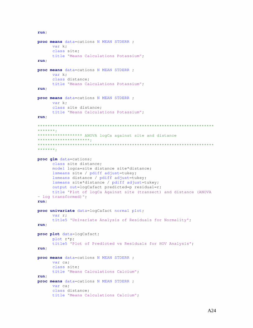
A24
run; proc means data=cations N MEAN STDERR ; var k; class site; title "Means Calculations Potassium"; run; proc means data=cations N MEAN STDERR ; var k; class distance; title "Means Calculations Potassium"; run; proc means data=cations N MEAN STDERR ; var k; class site distance; title "Means Calculations Potassium"; run; ******************************************************************************; ****************** ANOVA logCa against site and distance *********************; ******************************************************************************; proc glm data=cations; class site distance; model logca=site distance site*distance; lsmeans site / pdiff adjust=tukey; lsmeans distance / pdiff adjust=tukey; lsmeans site*distance / pdiff adjust=tukey; output out=logCafact predicted=p residual=r; title "Plot of logCa Against site (transect) and distance (ANOVA - log transformed)"; run; proc univariate data=logCafact normal plot; var r; title5 "Univariate Analysis of Residuals for Normality"; run; proc plot data=logCafact; plot r*p; title5 "Plot of Predicted vs Residuals for HOV Analysis"; run; proc means data=cations N MEAN STDERR ; var ca; class site; title "Means Calculations Calcium"; run; proc means data=cations N MEAN STDERR ; var ca; class distance; title "Means Calculations Calcium";

A25
run; proc means data=cations N MEAN STDERR ; var ca; class site distance; title "Means Calculations Calcium"; run; ******************************************************************************; ****************** ANOVA logMg against site and distance *********************; ******************************************************************************; proc glm data=cations; class site distance; model logmg=site distance site*distance; lsmeans site / pdiff adjust=tukey; lsmeans distance / pdiff adjust=tukey; lsmeans site*distance / pdiff adjust=tukey; output out=logMgfact predicted=p residual=r; title "Plot of logMg Against site (transect) and distance (ANOVA - log transformed)"; run; proc univariate data=logMgfact normal plot; var r; title5 "Univariate Analysis of Residuals for Normality"; run; proc plot data=logMgfact; plot r*p; title5 "Plot of Predicted vs Residuals for HOV Analysis"; run; proc means data=cations N MEAN STDERR ; var Mg; class site; title "Means Calculations Mg"; run; proc means data=cations N MEAN STDERR ; var Mg; class distance; title "Means Calculations Magnesium"; run; proc means data=cations N MEAN STDERR ; var Mg; class site distance; title "Means Calculations Magnesium"; run; ******************************************************************************; ****************** ANOVA logNa against site and distance *********************;
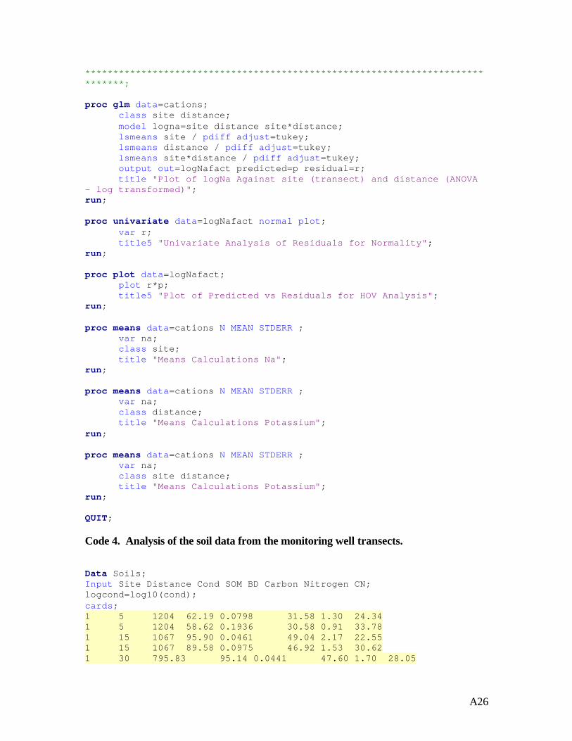
A26
******************************************************************************; proc glm data=cations; class site distance; model logna=site distance site*distance; lsmeans site / pdiff adjust=tukey; lsmeans distance / pdiff adjust=tukey; lsmeans site*distance / pdiff adjust=tukey; output out=logNafact predicted=p residual=r; title "Plot of logNa Against site (transect) and distance (ANOVA - log transformed)"; run; proc univariate data=logNafact normal plot; var r; title5 "Univariate Analysis of Residuals for Normality"; run; proc plot data=logNafact; plot r*p; title5 "Plot of Predicted vs Residuals for HOV Analysis"; run; proc means data=cations N MEAN STDERR ; var na; class site; title "Means Calculations Na"; run; proc means data=cations N MEAN STDERR ; var na; class distance; title "Means Calculations Potassium"; run; proc means data=cations N MEAN STDERR ; var na; class site distance; title "Means Calculations Potassium"; run; QUIT; Code 4. Analysis of the soil data from the monitoring well transects. Data Soils; Input Site Distance Cond SOM BD Carbon Nitrogen CN; logcond=log10(cond); cards; 1 5 1204 62.19 0.0798 31.58 1.30 24.34 1 5 1204 58.62 0.1936 30.58 0.91 33.78 1 15 1067 95.90 0.0461 49.04 2.17 22.55 1 15 1067 89.58 0.0975 46.92 1.53 30.62 1 30 795.83 95.14 0.0441 47.60 1.70 28.05
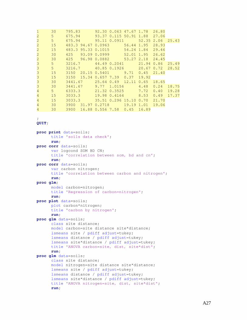
A27
1 30 795.83 92.30 0.063 47.67 1.78 26.80 2 5 675.94 93.37 0.115 50.91 1.88 27.06 2 5 675.94 95.11 0.0911 52.35 2.06 25.43 2 15 483.3 94.67 0.0963 56.44 1.95 28.93 2 15 483.3 95.33 0.1015 54.24 1.84 29.46 2 30 425 93.09 0.0999 52.01 1.95 26.62 2 30 425 96.98 0.0882 53.27 2.18 24.45 3 5 3216.7 44.49 0.2041 21.94 0.86 25.49 3 5 3216.7 40.85 0.1926 20.67 0.72 28.52 3 15 3150 20.15 0.5401 9.71 0.45 21.40 3 15 3150 15.34 0.657 7.39 0.37 19.92 3 30 3441.67 25.64 0.49 12.11 0.65 18.65 3 30 3441.67 9.77 1.0156 4.48 0.24 18.75 4 5 6333.3 21.32 0.3525 7.72 0.40 19.28 4 15 3033.3 19.98 0.4164 8.53 0.49 17.37 4 15 3033.3 35.51 0.296 15.10 0.70 21.70 4 30 3900 31.97 0.2718 19.19 1.01 19.06 4 30 3900 16.88 0.556 7.58 0.45 16.89 ; QUIT; proc print data=soils; title "soils data check"; run; proc corr data=soils; var logcond SOM BD CN; title "correlation between som, bd and cn"; run; proc corr data=soils; var carbon nitrogen; title "correlation between carbon and nitrogen"; run; proc glm; model carbon=nitrogen; title "Regression of carbon=nitrogen"; run; proc plot data=soils; plot carbon*nitrogen; title "carbon by nitrogen"; run; proc glm data=soils; class site distance; model carbon=site distance site*distance; lsmeans site / pdiff adjust=tukey; lsmeans distance / pdiff adjust=tukey; lsmeans site*distance / pdiff adjust=tukey; title "ANOVA carbon=site, dist, site*dist"; run; proc glm data=soils; class site distance; model nitrogen=site distance site*distance; lsmeans site / pdiff adjust=tukey; lsmeans distance / pdiff adjust=tukey; lsmeans site*distance / pdiff adjust=tukey; title "ANOVA nitrogen=site, dist, site*dist"; run;

A28
QUIT; ***************************************************************; **************** Regression logcond and SOM *******************; ***************************************************************; proc glm data=soils; model logcond=SOM; Title "conductivity by SOM"; output out=SOM predicted=p residual=r; title "Plot of Conductivity Against SOM (regression - log-transformed)"; run; proc univariate data=SOM normal plot; var r; title5 "Univariate Analysis of Residuals for Normality"; run; proc plot data=SOM; plot r*p; title5 "Plot of Predicted vs Residuals for HOV Analysis"; run; proc plot data=soils; plot logcond*SOM; Title "logcond by SOM"; run; proc plot data=soils; plot SOM*cond; Title "logcond by SOM"; run; proc plot data=soils; plot logcond*logSOM; Title "logcond by logSOM"; run; ****************************************************************************; ******************* Regression logcond and bulk density ********************; ****************************************************************************; proc glm data=soils; model logcond=BD; Title "conductivity by BD"; output out=BD predicted=p residual=r; title "Plot of Conductivity Against BD (regression - log-transformed)"; run; proc univariate data=BD normal plot; var r; title5 "Univariate Analysis of Residuals for Normality"; run;

A29
proc plot data=BD; plot r*p; title5 "Plot of Predicted vs Residuals for HOV Analysis"; run; proc plot data=soils; plot logcond*BD; Title "logcond by BD"; run; ****************************************************************************; ****************** Regression logcond by CN ratio **************************; ****************************************************************************; proc glm data=soils; model logcond=CN; Title "conductivity by CN"; output out=CN predicted=p residual=r; title "Plot of Conductivity Against CN (regression - log-transformed)"; run; proc univariate data=CN normal plot; var r; title5 "Univariate Analysis of Residuals for Normality"; run; proc plot data=CN; plot r*p; title5 "Plot of Predicted vs Residuals for HOV Analysis"; run; proc plot data=soils; plot logcond*CN; Title "logcond by CN"; run; ****************************************************************************; ********** Factorial ANOVA SOM AND site, distance and interaction *********; ****************************************************************************; proc glm data=soils; class site distance; model SOM=site distance site*distance; lsmeans site / pdiff adjust=tukey; lsmeans distance / pdiff adjust=tukey; lsmeans site*distance / pdiff adjust=tukey; output out=SOMfact predicted=p residual=r;

A30
title "Plot of SOM Against site distance and s*d(ANOVA - logCOND)"; run; proc univariate data=SOMfact normal plot; var r; title5 "Univariate Analysis of Residuals for Normality"; run; proc plot data=SOMfact; plot r*p; title5 "Plot of Predicted vs Residuals for HOV Analysis"; run; proc means data=soils N MEAN STDERR ; var SOM; class site; title "Means Calculations SOM"; run; proc means data=soils N MEAN STDERR ; var SOM; class distance; title "Means Calculations SOM"; run; proc means data=soils N MEAN STDERR ; var SOM; class site distance; title "Means Calculations SOM"; run; ****************************************************************************; ********** Factorial ANOVA bd and site, dist, site*dist *******************; ****************************************************************************; proc glm data=soils; class site distance; model bd=site distance site*distance; lsmeans site / pdiff adjust=tukey; lsmeans distance / pdiff adjust=tukey; lsmeans site*distance / pdiff adjust=tukey; output out=BDfact predicted=p residual=r; title "Plot of BD Against site distance and s*d(ANOVA - logCOND)"; run; proc univariate data=BDfact normal plot; var r; title5 "Univariate Analysis of Residuals for Normality"; run; proc plot data=BDfact; plot r*p; title5 "Plot of Predicted vs Residuals for HOV Analysis"; run;

A31
proc means data=soils N MEAN STDERR ; var BD; class site; title "Means Calculations bd"; run; proc means data=soils N MEAN STDERR ; var bd; class distance; title "Means Calculations bd"; run; proc means data=soils N MEAN STDERR ; var bd; class site distance; title "Means Calculations BD"; run; ****************************************************************************; *********** Factorial ANOVA CN and site, dist and s*d *********************; ****************************************************************************; proc glm data=soils; class site distance; model CN=site distance site*distance; lsmeans site / pdiff adjust=tukey; lsmeans distance / pdiff adjust=tukey; lsmeans site*distance / pdiff adjust=tukey; output out=CNfact predicted=p residual=r; title "Plot of CN Against site distance and s*d(ANOVA - logCOND)"; run; proc univariate data=CNfact normal plot; var r; title5 "Univariate Analysis of Residuals for Normality"; run; proc plot data=CNfact; plot r*p; title5 "Plot of Predicted vs Residuals for HOV Analysis"; run; proc means data=soils N MEAN STDERR ; var CN; class site; title "Means Calculations CN"; run; proc means data=soils N MEAN STDERR ; var CN; class distance; title "Means Calculations CN"; run; proc means data=soils N MEAN STDERR ; var CN;

A32
class site distance; title "Means Calculations CN"; run; QUIT; proc plot data=soils; plot cond*SOM; title "conductivity by som"; run; proc plot data=soils; plot cond*BD; title "conductivity by BD"; run; proc plot data=soils; plot cond*CN; title "conductivity by CN"; run; proc plot data=soils; plot logcond*SOM; title "conductivity by som"; run; proc plot data=soils; plot logcond*BD; title "conductivity by BD"; run; proc plot data=soils; plot logcond*CN; title "conductivity by CN"; run; proc reg data=soils; model logcond=SOM; run; proc reg data=soils; model logcond=BD; run; proc reg data=soils; model logcond=CN; run; QUIT;