1

Appendix to

“Making It Personal: The Role of Leader-Specific

Signals in Extended Deterrence”

By Roseanne W. McManus

Table of Contents

1. Summary Statistics 2

2. Fuller Results from the “Results” Section 3

3. Robustness Checks 10

4. Further Explanation of Matching 21

5. Sources for Coding Visits 23

6. Dictionary and Examples for Coding Statements of Support 26

2

Part 1: Summary Statistics

Table A1: Summary Statistics for Key Variables

Variable Mean Std. Dev. Min Max Violent MID Initiation 0.009 0.095 0 0 Any MID Initiation 0.013 0.115 0 0 Fatal MID Initiation 0.004 0.065 0 0 Major Power Visit to State B 0.275 0.446 0 0 Major Power Defense Pact with State B 0.516 0.500 1 0 Major Power Nuclear Deployment in State B 0.159 0.365 0 0 Contiguity (States A & B) 0.252 0.434 0 0 Distance (States A & B) 3.071 2.685 2.351 0.005 Capabilities, State A 0.041 0.060 0.010 0.00002 Capabilities, State B 0.010 0.014 0.003 0.00002 Relative Capabilities 0.472 0.207 0.498 0.002 Democracy, State A 0.455 0.498 0 0 Democracy, State B 0.453 0.498 0 0 Joint Democracy 0.223 0.416 0 0 Peace Years (between Violent MIDs) 30.012 29.586 22 0 US President Visit to State B 0.139 0.346 0 0 US Hosting State B’s Leader 0.347 0.476 0 0 US Statements of Support for State B 0.371 0.483 0 0

Note: These statistics are from my sample of politically-relevant dyads, with the US, Russia, and China dropped as State B.

3

Part 2: Fuller Results from the “Results” Section

Table A2: Tests of Hypotheses 1-3 with Control Variables Results Shown

(1) (2) (3) (4) Violent MID Any MID Fatal MID Violent MID

(US Signals Only) Major Power -0.194*** -0.155*** -0.109* Visit to State B (0.048) (0.040) (0.058) Major Power Defense -0.055 -0.022 -0.244*** Pact with State B (0.059) (0.053) (0.077) Major Power Nuclear 0.002 -0.073 0.195 Deployment in State B (0.095) (0.089) (0.137) US President -0.237*** Visit to State B (0.064) US Hosting State B’s 0.024 Leader (0.040) US Statements of 0.124** Support for State B (0.049) US Defense Pact 0.106 with State B (0.079) US Nuclear -0.078 Deployment in State B (0.101) Land Contiguity 0.587*** 0.549*** 0.818*** 0.583*** (States A & B) (0.069) (0.062) (0.104) (0.071) Distance -0.097*** -0.107*** -0.079*** -0.121*** (States A & B) (0.021) (0.018) (0.030) (0.026) Capabilities, 1.908*** 2.403*** 1.686*** 2.075*** State A (0.429) (0.405) (0.554) (0.579) Capabilities, 8.906*** 8.884*** 5.221 5.277* State B (2.586) (2.482) (4.484) (2.789)

4

Relative -0.472** -0.413** -0.545* -0.207 Capabilities (0.215) (0.193) (0.330) (0.338) Democracy, 0.005 0.071 0.079 -0.033 State A (0.070) (0.061) (0.077) (0.070) Democracy, 0.179** 0.188*** 0.119 0.124 State B (0.082) (0.067) (0.117) (0.084) Joint -0.523*** -0.508*** -0.671*** -0.498*** Democracy (0.099) (0.087) (0.136) (0.103) Peace -0.056*** -0.059*** -0.059*** -0.070*** Years (0.006) (0.004) (0.006) (0.007) Peace Years 0.001*** 0.001*** 0.001*** 0.001*** Squared (0.000) (0.000) (0.000) (0.000) Peace Years -0.000*** -0.000*** -0.000*** -0.000*** Cubed (0.000) (0.000) (0.000) (0.000) Year of Observation 0.001 0.003** -0.001 -0.001 (0.001) (0.001) (0.002) (0.001) Observations 93,258 93,243 93,293 86,119

Note: * p < .10, ** p < .05, *** p < .01. These are probit models with standard errors clustered by dyad. The leader-specific signal variables are lagged.

5

Table A3: Additional Individual Major Power Models (1) (2) (3) (4) UK France Russia China Visit to State B by Major -0.071 0.003 -0.235** -0.100 Power at Top of Column (0.079) (0.081) (0.096) (0.082) State B Pact with Major -0.306*** -0.238*** -0.269** 0.364 Power at Top of Column (0.082) (0.082) (0.121) (0.234) State B Nukes from Major 0.107 -0.004 Power at Top of Column (0.240) (0.249) Observations 78,849 78,844 86,133 86,128

Note: * p < .10, ** p < .05, *** p < .01. These are probit models with standard errors clustered by dyad. The dependent variable in each model is Violent MID Initiation. The leader-specific signal variables are lagged. The control variable results are omitted to save space.

Table A4: Dropping Some Major Powers from the Main Visit Compilation Measure (1) (2) (3) Drop UK

Visits Drop French

Visits Drop Chinese

Visits Major Power -0.178*** -0.237*** -0.185*** Visit to State B (0.047) (0.048) (0.053) Major Power Defense -0.056 -0.050 -0.055 Pact with State B (0.059) (0.059) (0.059) Major Power Nuclear -0.002 -0.006 0.001 Deployment in State B (0.096) (0.097) (0.095) Observations 93,258 93,258 93,258

Note: * p < .10, ** p < .05, *** p < .01. These are probit models with standard errors clustered by dyad. The dependent variable in each model is Violent MID Initiation. The leader-specific signal variables are lagged. The control variable results are omitted to save space.

6

Table A5: Average Marginal Effects from Model 1

Variable Avg. Marginal

Effect Std. Err. P-value Major Power Visit to State B -0.0040 0.001 0.000 Major Power Pact with State B -0.0011 0.001 0.347 Nuclear Deployment in State B 0.00004 0.002 0.984 Contiguity 0.012 0.002 0.000 Distance -0.002 0.000 0.000 Capabilities, State A 0.040 0.009 0.000 Capabilities, State B 0.185 0.056 0.001 Relative Capabilities -0.010 0.005 0.031 Democracy, State A 0.0001 0.001 0.944 Democracy, State B 0.004 0.002 0.034 Joint Democracy -0.011 0.002 0.000 Peace Years -0.001 0.00015 0.000 Peace Years Squared 0.00002 0.000004 0.000 Peace Years Cubed -0.0000001 0.00000002 0.002 Year of Observation 0.00001 0.00003 0.650

7

Table A6: Countries Where Visits Are Predicted to Have the Largest Deterrent Effect

Visit Recipient Number of Appearances in Top 1% Marginal Effects

India 78 West Germany 41 Turkey 23 Israel 18 Pakistan 12 South Korea 11 Poland 7 Myanmar/Burma 6 Canada 5 Czechoslovakia 5 Thailand 5 Moldova 4 Mongolia 4 North Korea 4 Vietnam 4

Note: This table summarizes which visit recipients most frequently had among the top one percent largest (i.e., most negative) marginal effects of a visit. I predicted the marginal effect of the Major Power Visit variable for each observation in the sample based on Model 1, dropped observations in which no visit took place, and then ranked the remaining observations by marginal effect size.

8

Table A7: Tests for Hypotheses 4-5 with Control Variable Results Shown (1) (2) Testing H4 Testing H5 Major Power Leader -0.105* Visit to State B (0.062) Major Power Pact -0.030 with State B (0.060) Visit X Pact -0.166* (0.085) Major Power Nuclear 0.020 Deployment in State B (0.096) US President 0.020 Visit to State B (0.154) US Statements of 0.134*** Support for State B (0.049) US Visit X US -0.300* Statements (0.160) US Hosting State B’s 0.027 Leader (0.040) US Defense Pact with 0.106 State B (0.078) US Nuclear -0.082 Deployment in State B (0.101) Land Contiguity 0.582*** 0.582*** (States A & B) (0.069) (0.070) Distance -0.096*** -0.121*** (States A & B) (0.020) (0.026) Capabilities, 1.887*** 2.065*** State A (0.430) (0.579) Capabilities, 8.904*** 5.240* State B (2.553) (2.799)

9

Relative -0.455** -0.201 Capabilities (0.215) (0.338) Democracy, 0.004 -0.034 State A (0.070) (0.070) Democracy, 0.174** 0.122 State B (0.083) (0.084) Joint -0.518*** -0.496*** Democracy (0.099) (0.103) Peace -0.056*** -0.070*** Years (0.006) (0.007) Peace Years 0.001*** 0.001*** Squared (0.000) (0.000) Peace Years -0.000*** -0.000*** Cubed (0.000) (0.000) Year of Observation 0.001 -0.001 (0.001) (0.001) Observations 93,258 86,119

10

Part 3: Robustness Checks

Table A8: Breaking Down Visits Variable

(1) (2) (3) By Current

and Former Leaders

By Democratic and Autocratic

Leaders

By Leaders with and without

Military Background

Major Power Visit to State B -0.153*** under Current Leader (0.047) Major Power Visit to State B 0.007 under Previous Leader (0.048) Major Power Visit to State B -0.120** by Democratic Leader (0.053) Major Power Visit to State B -0.237*** by Autocratic Leader (0.066) Major Power Visit to State B -0.125** by Leader with Military Background (0.056) Major Power Visit to State B -0.323*** by Leader without Mil. Background (0.072) Major Power Defense -0.074 -0.053 -0.069 Pact with State B (0.059) (0.059) (0.062) Major Power Nuclear 0.020 -0.003 0.005 Deployment in State B (0.094) (0.096) (0.100) Observations 86,342 93,258 80,417

Note: * p < .10, ** p < .05, *** p < .01. These are probit models with standard errors clustered by dyad. The dependent variable in each model is Violent MID Initiation. The leader-specific signal variables are lagged. The control variable results are omitted to save space. Model 4 has fewer observations because of the five-year aggregation, and Model 6 has fewer observations because of time limitations on the availability of the leader background data.

11

Table A9: Controlling for Affinity

(1) (2) (3) All Major

Powers US Russia

Visit to State B -0.187*** -0.223*** -0.234** (0.048) (0.063) (0.094) Pact with State B -0.071 0.135* -0.269** (0.059) (0.081) (0.122) Nukes Deployed 0.011 -0.061 0.001 in State B (0.094) (0.103) (0.249) Affinity with State B -0.388* -0.182** -0.014 (0.203) (0.073) (0.078) Hosting State B’s 0.039 Leader (0.041) Statements of Support 0.131*** for State B (0.049) Observations 92,985 85,872 85,886

Note: * p < .10, ** p < .05, *** p < .01. These are probit models with standard errors clustered by dyad. The dependent variable in each model is Violent MID Initiation. The leader-specific signal variables are lagged. The control variable results are omitted to save space. In Model 1, the highest affinity score with any major power is used. Models 2 and 3 use the affinity scores with the US and Russia, respectively.

12

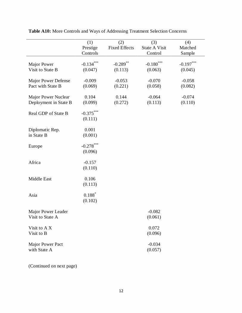
Table A10: More Controls and Ways of Addressing Treatment Selection Concerns (1) (2) (3) (4) Prestige

Controls Fixed Effects State A Visit

Control Matched Sample

Major Power -0.134*** -0.289** -0.180*** -0.197*** Visit to State B (0.047) (0.113) (0.063) (0.045) Major Power Defense -0.009 -0.053 -0.070 -0.058 Pact with State B (0.069) (0.221) (0.058) (0.082) Major Power Nuclear 0.104 0.144 -0.064 -0.074 Deployment in State B (0.099) (0.272) (0.113) (0.110) Real GDP of State B -0.375*** (0.111) Diplomatic Rep. 0.001 in State B (0.001) Europe -0.278*** (0.096) Africa -0.157 (0.110) Middle East 0.106 (0.113) Asia 0.188* (0.102) Major Power Leader -0.082 Visit to State A (0.061) Visit to A X 0.072 Visit to B (0.096) Major Power Pact -0.034 with State A (0.057) (Continued on next page)

13

Major Power Nuclear -0.063 Deployment in State A (0.102)

Observations 86,643 14,874 71,293 73,999

Note: * p < .10, ** p < .05, *** p < .01. These are probit models with standard errors clustered by dyad. The dependent variable in each model is Violent MID Initiation. The leader-specific signal variables are lagged. Except for new controls, the control variable results are omitted to save space. The comparison category for the dummies in Model 1 is the Americas. In Model 3, dyads in which State A is the US, Russia, or China are dropped.

14

Table A11: Separate Regressions Showing Tourism Appeal Is a Good Exclusion Restriction (1) (2) Predicting

Visits Predicting MID

Initiation Tourism Appeal 0.031*** -0.002 (0.001) (0.003) Major Power Defense 0.177*** -0.062 Pact with State B (0.026) (0.064) Major Power Nuclear 0.038** 0.031 Deployment in State B (0.019) (0.102) Capabilities, 16.124*** 9.742*** State B (0.459) (2.948) Democracy, 0.050** 0.192** State B (0.022) (0.084) Years without State B -0.005 MID Involvement (0.005) Year 0.019*** -0.000 (0.001) (0.001) Major Power Leader -0.181*** Visit to State B (0.047) Land Contiguity, 0.598*** States A & B (0.075) Distance, States A & B -0.098*** (0.022) Capabilities, State A 1.912*** (0.458) Relative Capabilities, -0.376 States A & B (0.229) Democracy, State A 0.019 (0.071)

15

Joint Democracy, -0.509*** States A & B (0.100) Peace Years, -0.056*** States A & B (0.006) Peace Years Squared 0.001*** (0.000) Peace Years Cubed -0.000*** (0.000)

Observations 89,073 89,818

Note: * p < .10, ** p < .05, *** p < .01. These are probit models with standard errors clustered by dyad. In Model 1, all of the predictors are lagged because the visits variable itself is lagged. In Model 2, only the leader-specific signal variables are lagged.

Table A12: Bivariate Probit Model Stage 1: Predicting Major

Power Leader Visit Stage 2: Predicting

Violent MID Initiation Major Power Leader -0.548*** Visit to State B (0.174) Tourism Appeal 0.031*** (0.001) Major Power Defense 0.176*** -0.041 Pact with State B (0.026) (0.066) Major Power Nuclear 0.038** 0.061 Deployment in State B (0.019) (0.095) Capabilities, 16.138*** 12.142*** State B (0.458) (3.200) Democracy, 0.051** 0.191** State B (0.022) (0.083)

16

Years without State B -0.005 MID Involvement (0.005) Year 0.019*** 0.001 (0.001) (0.002) Land Contiguity, 0.575*** States A & B (0.073) Distance, States A & B -0.096*** (0.021) Capabilities, State A 1.795*** (0.448) Relative Capabilities, -0.328 States A & B (0.220) Democracy, State A 0.018 (0.070) Joint Democracy, -0.490*** States A & B (0.100) Peace Years, -0.057*** States A & B (0.006) Peace Years Squared 0.001*** (0.000) Peace Years Cubed -0.000*** (0.000) Correlation between equations (ρ) = 0.216 χ2 for 𝜌𝜌 = 4.884 p-value for χ2 = 0.027

Observations = 89,073

Note: * p < .10, ** p < .05, *** p < .01. These are two equations from the same bivariate probit model. In Stage 1, all of the predictors are lagged because the visits variable itself is lagged. In Stage 2, only the leader-specific signals are lagged. Standard errors are clustered by dyad.

17

Table A13: Different Dependent Variable and Types of Visits (1) (2) (3) MCT DV Dropping

Summits Capturing Duration

Major Power Leader -0.218* Visit (0.126) US Presidential Visit -0.261*** (not counting summits) (0.067) US Presidential Visit -0.062*** Duration (0.022) Major Power/US -0.147 0.106 0.104 Defense Pact (0.092) (0.078) (0.079) Major Power/US -0.042 -0.081 -0.080 Nuclear Deployment (0.175) (0.101) (0.101) US Hosting State B’s 0.023 0.023 Leader (0.040) (0.040) US Support Words 0.124** 0.114** (0.049) (0.050) Observations 78,133 86,119 86,119

Note: * p < .10, ** p < .05, *** p < .01. These are probit models with standard errors clustered by dyad. The dependent variable in Model 1 is Militarized Compellent Threat, and the dependent variable in Models 2-3 is Violent MID Initiation. The leader-specific signal variables are lagged. The control variable results are omitted to save space.

18

Table A14: Different Samples (1) (2) (3) (4) All Dyads Dyads with

MID in Last 15 Years

Cold War Post-Cold War

Major Power -0.373*** -0.111** -0.173*** -0.126* Visit to State B (0.113) (0.053) (0.067) (0.067) Major Power Defense -0.097 -0.106 -0.024 -0.042 Pact with State B (0.153) (0.072) (0.070) (0.087) Major Power Nuclear 0.302 -0.088 0.051 -0.329* Deployment (0.228) (0.126) (0.102) (0.182) Observations 959,462 14,238 50,022 43,236 Note: * p < .10, ** p < .05, *** p < .01. These are probit models with standard errors clustered by dyad. The dependent variable in each model is Violent MID Initiation. The leader-specific signal variables are lagged. The control variable results are omitted to save space.

19

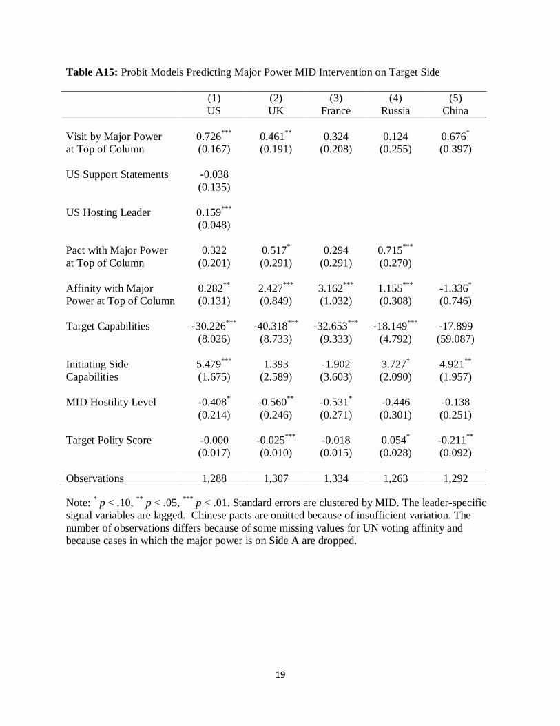
Table A15: Probit Models Predicting Major Power MID Intervention on Target Side

(1) (2) (3) (4) (5) US UK France Russia China Visit by Major Power 0.726*** 0.461** 0.324 0.124 0.676* at Top of Column (0.167) (0.191) (0.208) (0.255) (0.397) US Support Statements -0.038 (0.135) US Hosting Leader 0.159*** (0.048) Pact with Major Power 0.322 0.517* 0.294 0.715*** at Top of Column (0.201) (0.291) (0.291) (0.270) Affinity with Major 0.282** 2.427*** 3.162*** 1.155*** -1.336* Power at Top of Column (0.131) (0.849) (1.032) (0.308) (0.746) Target Capabilities -30.226*** -40.318*** -32.653*** -18.149*** -17.899 (8.026) (8.733) (9.333) (4.792) (59.087) Initiating Side 5.479*** 1.393 -1.902 3.727* 4.921** Capabilities (1.675) (2.589) (3.603) (2.090) (1.957) MID Hostility Level -0.408* -0.560** -0.531* -0.446 -0.138 (0.214) (0.246) (0.271) (0.301) (0.251) Target Polity Score -0.000 -0.025*** -0.018 0.054* -0.211** (0.017) (0.010) (0.015) (0.028) (0.092) Observations 1,288 1,307 1,334 1,263 1,292

Note: * p < .10, ** p < .05, *** p < .01. Standard errors are clustered by MID. The leader-specific signal variables are lagged. Chinese pacts are omitted because of insufficient variation. The number of observations differs because of some missing values for UN voting affinity and because cases in which the major power is on Side A are dropped.

20

Table A16: Tests Not Mentioned in Paper (1) (2) (3) (4) (5) Include

Joiners Drop

Ongoing MID & Target-Initiator Dyads

Drop Britain and France as Potential

Targets

Rare Events Logit

ATOP Pact Measure

Major Power -0.194*** -0.203*** -0.188*** -0.466*** -0.215*** Visit to State B (0.048) (0.053) (0.051) (0.125) (0.052) Major Power Defense -0.054 -0.063 -0.043 -0.133 -0.058 Pact with State B (0.059) (0.062) (0.062) (0.151) (0.056) Major Power Nuclear 0.001 0.009 -0.028 0.010 -0.001 Deployment (0.095) (0.101) (0.116) (0.256) (0.098) Observations 93,437 91,372 78,598 93,258 80,417

Note: * p < .10, ** p < .05, *** p < .01. These are probit models with standard errors clustered by dyad. The dependent variable in each model is Violent MID Initiation. The leader-specific signal variables are lagged. The control variable results are omitted to save space.

21

Part 4: Further Explanation of Matching

I use Coarsened Exact Matching (CEM), which creates a completely balanced sample

based on coarsened versions of the variables used in matching (Iacus, King, and Porro 2012).

Coarsening the variables means establishing cutpoints in the range of values taken by each

variable so that all values between any given pair of cutpoints are substantively similar enough to

be treated as equal for purposes of matching. After coarsening, the CEM algorithm creates strata

that contain all observations with equivalent values of the coarsened variables. Strata that do not

contain at least one treated observation and one control observation are dropped, and

observations in these strata are not included in the matched sample. Since some strata are likely

to contain more than one of each type of observation, the algorithm also assigns weights to

account for the size of the strata, and later regressions on the matched sample must take into

account these weights. Although coarsened variables are used for matching, the original

variables are used for regressions in the matched sample.

The most crucial decision to make in the matching process is which variables to use for

matching. I match on variables related to State B's closeness to a major power as well as State

B's probability of being targeted in a MID. The first variable used in matching is State B’s

region. State B's region is likely to reflect its international prestige, which might make it a more

or less desirable visit location, and also affects its probability of being targeted in a MID, since

some regions are more conflict-prone than others. Second, I match on State B's CINC score.

States with a higher CINC score might be more likely to receive visits because they are more

important in the international system and less likely to be targeted in MIDs because they are

harder to defeat. Third, I match on State B's regime type. Democratic states might be more

22

likely to receive visits from democratic leaders and less likely to be targeted in MIDs by other

democracies. Fourth, I match on State B's maximum level of affinity with any major power,

calculated based on UN voting similarity. Major powers are more likely to visit and also more

likely to militarily assist countries they have higher affinity with. Fifth, I match on an indicator

for whether State B has a major power defense pact. Defense pacts increase the likelihood of

both visits and military assistance in a similar way to affinity. Finally, I also match on the

number of years since State B last became involved in a MID. Countries that have more recently

been involved in a MID may be less likely to be visited and more likely to be targeted in a MID

again. While I cannot claim that I have included every possible factor that might influence how

major powers relate to weaker states, I have included the most relevant factors that are easily

observable.

With regard to coarsening, defense pact and regime type are dummies and cannot be

further coarsened. The region variable, which is categorical, is not further coarsened either,

meaning that each state is matched with another in its own region. The continuous Affinity and

CINC score variables are coarsened into four and seven categories, respectively. These

categories become narrower at higher levels of these variables, where I expect small differences

to matter more for predicting visits and MID initiation. The count of years since State B’s last

MID is coarsened into four categories: 0 years, 1 year, 2 years, and more than 2 years. In making

decisions about coarsening, my goal was to make the categories narrow enough to have valid

matches, but not so narrow as to make it impossible to find matches in most cases.

23

Part 5: Sources for Coding Visits

I identified the leaders whose travels we searched for based primarily on:

Goemans, H.E., Kristian Skrede Gleditsch, and Giacomo Chiozza. 2009. “Introducing Archigos: A Data Set of Political Leaders.” Journal of Peace Research 46(2):269-183. Version 4.1.

However, I diverged from Archigos on the leader’s identity in some cases because Archigos codes the leader with primary decision-making power, but in the case of Russia and China in some years, the primary decision-maker almost never traveled abroad. Therefore, I coded travels by the official head of state, rather than the primary decision-maker, in the following instances:

• I code Medvedev’s travel for his entire term as Russian president. • I code Zhou Enlai’s travel as Chinese head of state, 1950-1976. • I code Hua Guofeng’s travel as Chinese head of state, 1976-1980. • I code Zhao Ziyang’s travel as Chinese head of state, 1980-1992.

My research assistant and I used the following sources to search for visits:

United States

• All years: Department of State. 2015. “Travels of the President.” http://history. state.gov/departmenthistory/travels/president (March 14, 2014 - January 2, 2015).

Britain

• 1950-1985: FBIS and ProQuest Historical Newspapers* • 1986-May 2010: Lexis-Nexis • 1979-1990: Margaret Thatcher Foundation. 2016. “Speeches, Interviews, and Other

Statements.” http://www.margaretthatcher.org/speeches/default.asp (July 27, 2016). • 1990-1997: Major, John. 2016. “Chronology” and “Speeches/Statements.”

http://www.johnmajor.co.uk/chronology.html, http://www.johnmajor.co.uk/page1597.html (July 26, 2016).

• May-Dec 2010: Sedghi, Ami. 2015. “David Cameron's Overseas Trips: Where Has He Visited?” Guardian, March 11. http://www.theguardian.com/news/datablog/2015/mar/11/david-camerons-trips-overseas-where-has-he-visited (June 24, 2016).

France

• 1950-1985: FBIS and ProQuest Historical Newspapers • 1986-2010: Lexis-Nexis

24

China

• 1950-1981: FBIS and ProQuest Historical Newspapers • 1950-1963: Foreign Ministry of the People’s Republic of China. 2016. “Premier Zhou

Enlai's Three Tours of Asian and African Countries.” http://www.fmprc.gov.cn/mfa_eng/ziliao_665539/3602_665543/3604_665547/t18001.shtml (June 26, 2016).

• 1965: Wilson Center Digital Archives. http://digitalarchive.wilsoncenter.org/document/113055 (June 27, 2016).

• 1982-2010: Li, Xiaoting. 2015. “Dealing with the Ambivalent Dragon: Can Engagement Moderate China’s Strategic Competition with America?” International Interactions 41:480-508. Unlike Li, I count visits by only one leader, initially the premier and then the president starting in 1993. I also count visits to attend summits.

Russia

• 1950-1985: FBIS and ProQuest Historical Newspapers • 1964-1982: Associated Press. 1982. “Chronology of Brezhnev’s Life.” Pittsburgh

Press, November 11, A-12. https://news.google.com/newspapers?nid=1144&dat=19821110&id=ojM0AAAAIBAJ&sjid=BmAEAAAAIBAJ&pg=4168,4843941&hl=en (July 11, 2016).

• 1986-Aug 1991: Lexis-Nexis • Yeltsin years: Wikipedia. “List of Trips Made by Boris Yeltsin.”

https://en.wikipedia.org/wiki/List_of_trips_made_by_Boris_Yeltsin (June 25, 2016). • Putin years: Wikipedia. “List of International Trips Made by Vladimir Putin.”

https://en.wikipedia.org/wiki/List_of_international_trips_made_by_Vladimir_Putin (June 25, 2016).

• Medvedev years: Wikipedia. “Зарубежные поездки президента Медведева.” (Foreign Trips of President Medvedev.) https://ru.wikipedia.org/wiki/%D0%97%D0%B0%D1%80%D1%83%D0%B1%D0%B5%D0%B6%D0%BD%D1%8B%D0%B5_%D0%BF%D0%BE%D0%B5%D0%B7%D0%B4%D0%BA%D0%B8_%D0%BF%D1%80%D0%B5%D0%B7%D0%B8%D0%B4%D0%B5%D0%BD%D1%82%D0%B0_%D0%9C%D0%B5%D0%B4%D0%B2%D0%B5%D0%B4%D0%B5%D0%B2%D0%B0 (June 25, 2016).

* The ProQuest Historical Newspapers database that I searched included the following newspapers: American Israelite (1854-2000); Atlanta Daily World (1931-2003); Austin American Statesman (1871-1976); Baltimore Afro-American (1893-1988); Baltimore Sun (1837-1990); Boston Globe (1872-1984); Call and Post (Cleveland) (1934-1991); Chicago Defender (1909-1975); Chicago Tribune (1849-1992); Christian Science Monitor (1908-2003); Cleveland

25

Call & Post (1934-1991); Globe & Mail (1844-2012); Guardian and the Observer (1791-2003); Irish Times (1859-2012); Jerusalem Post (1932-2008); Jewish Advocate (1905-1990); Jewish Exponent (1887-1990); Los Angeles Sentinel (1934-2005); Los Angeles Times (1881-1992); New York Amsterdam News (1922-1993); New York Times (1851-2013); New York Tribune (1841-1962); Newsday (1940-1987); Norfolk Journal and Guide (1921-2003); Philadelphia Tribune (1912-2001); Pittsburgh Courier (1911-2002); Scotsman (1817-1950); South China Morning Post (1903-1997); Times of India (1838-2006); Toronto Star (1894-2011); Wall Street Journal (1889-1999); Washington Post (1877-1999).

26

Part 6: Dictionary and Examples for Coding Statements of Support

The follow words are in the dictionary used to measure statements of support. All words are weighted equally. Asterisks denote wildcards.

alliance*

allies

ally

alongside

assist*

deepen*

defend

friend*

joint*

multilateral

neighbor*

partner*

protect*

safeguard*

solidarity

support*

treaties

treaty

warm*

27

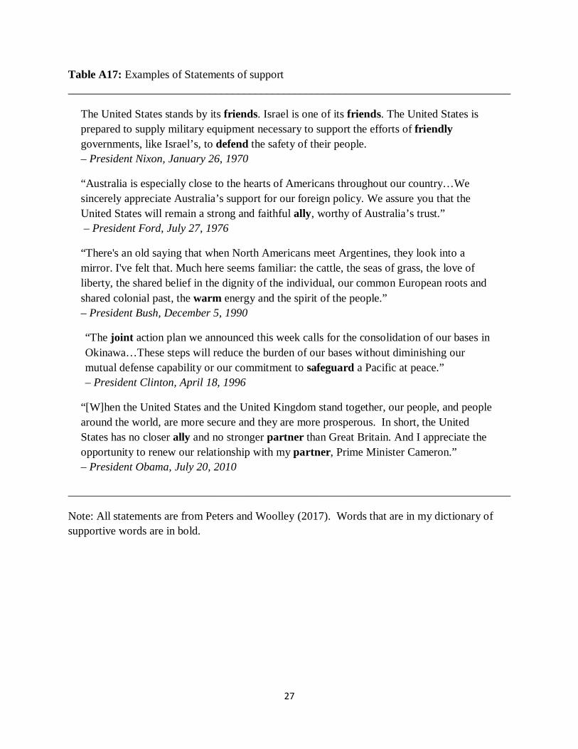
Table A17: Examples of Statements of support ______________________________________________________________________________

The United States stands by its friends. Israel is one of its friends. The United States is prepared to supply military equipment necessary to support the efforts of friendly governments, like Israel’s, to defend the safety of their people. – President Nixon, January 26, 1970

“Australia is especially close to the hearts of Americans throughout our country…We sincerely appreciate Australia’s support for our foreign policy. We assure you that the United States will remain a strong and faithful ally, worthy of Australia’s trust.” – President Ford, July 27, 1976

“There's an old saying that when North Americans meet Argentines, they look into a mirror. I've felt that. Much here seems familiar: the cattle, the seas of grass, the love of liberty, the shared belief in the dignity of the individual, our common European roots and shared colonial past, the warm energy and the spirit of the people.” – President Bush, December 5, 1990

“The joint action plan we announced this week calls for the consolidation of our bases in Okinawa…These steps will reduce the burden of our bases without diminishing our mutual defense capability or our commitment to safeguard a Pacific at peace.” – President Clinton, April 18, 1996

“[W]hen the United States and the United Kingdom stand together, our people, and people around the world, are more secure and they are more prosperous. In short, the United States has no closer ally and no stronger partner than Great Britain. And I appreciate the opportunity to renew our relationship with my partner, Prime Minister Cameron.” – President Obama, July 20, 2010

______________________________________________________________________________

Note: All statements are from Peters and Woolley (2017). Words that are in my dictionary of supportive words are in bold.