applying auto-regressive binomial model to … auto-regressive binomial model to ... lag markov...
TRANSCRIPT
Applying Auto-Regressive Binomial Model to
Forecast Economic Recession in U.S. and Sweden
Submitted by: Chunshu Zhao
Yamei Song
Supervisor: Md. Moudud Alam
D-level essay in Statistics, June 2010.
School of Technology & Business Studies, Dalarna University
Contents
ABSTRACT..................................................................................................................1
1 Introduction...............................................................................................................2
1.1 Background .......................................................................................................2
1.2 Aim....................................................................................................................4
2 Data and Methods .....................................................................................................4
2.1 Data description ................................................................................................4
2.1.1 The recession indicator ...........................................................................5
2.1.2 The explanatory variables .......................................................................5
2.2 Methods.............................................................................................................7
2.2.1 AR logit model........................................................................................7
2.2.2 Parameters estimation .............................................................................8
2.2.3 Parameters test ......................................................................................10
2.2.4 Forecasting............................................................................................10
2.2.5 Model selection criteria.........................................................................12
3 Results ......................................................................................................................12
3.1 Model selection and in-sample results ............................................................12
3.1.1 Empirical analysis to U.S......................................................................12
3.1.2 Empirical analysis to Sweden ...............................................................16
3.2 Out-of-sample results......................................................................................19
3.2.1 Out-of-sample results of U.S. ...............................................................19
3.2.2 Out-of-sample results of Sweden..........................................................21
4 Conclusion ...............................................................................................................23
References ...................................................................................................................26
1
ABSTRACT
In this paper, we construct an auto-regressive (AR) logit model which can be
applied in the prediction of the U.S. and Sweden economic recessions. The predictive
variables of this model vary between U.S. and Sweden. The predicted power of this
AR logit model is checked in terms of in-sample and out-of-sample performance. We
find that the goodness-of-fit of this model to data is remarkable and this model can
give reasonable degree of accuracy in the predicting U.S. and Sweden business cycle.
Keywords: Auto-regressive logit model, Business cycle, Recession
2
1 Introduction
1.1 Background
The latest recession in U.S. occurred ever since the bankruptcy of Lehman
Brothers Holding Inc. due to the sub prime mortgage crisis in 2008 and lasted more
than two years. The consequence of this recession is quite significant which is viewed
through several economic performance indicators, e.g. 10% unemployment rate and a
deeply decline of real GDP. Although nowadays the government of U.S. declares that
the recession in U.S. has end, the economy in Europe is experiencing a new round of
sharply decline, such as the 2010 Euro crisis including Greece, Ireland, Spain, and
Portugal. Thus, how to find an efficient ways to model and forecast economic
recession is nowadays a popular topic among policy makers and researchers. A binary
AR model has been considered as a useful model to forecast economic recession in
U.S., thus we want to investigate whether this kind of model is also applicable in
European countries such as Sweden.
Before going through the definition of recession, it is necessary to introduce a
general idea about business cycle, since recession is regarded as a part of business
cycle. In the view of macroeconomics, business cycle is a well-known financial
variable to measure the economy-wide fluctuations in production over a long period.
These fluctuations exit when the economic environment changes from an expansion
to a recession and vice versa. Generally, people are more concerned with recession
rather than expansion, since a majority of papers are focus on discussing recession.
The definition of recession varies between different research institutes and therefore
no exact definition of recession exists. One commonly used definition is provided by
the National Bureau of Economic Research (NBER) in US. In their words, “a
recession is a significant decline in economic activity spread across the economy,
lasting more than a few months, normally visible in real GDP, real income,
3
employment, industrial production, and wholesale-retail sales”1. From this definition,
we can see that being able to describe and predict a recession is of great interest for
the people. More specifically, policy makers who work on macroeconomic issues are
more concern with the trend of real GDP and real income, since a wrong prediction of
the future of economic state leads to the ineffective of policy itself. And the
employees in industry are mostly interested in the state of employment, and so on.
Thus, a reasonable assessment of economic activities such as business cycle is of
great importance to the whole society.
In modeling recession, AR binomial model has been found very useful. Kauppi
and Saikkonen (2005) predict U.S. recessions with dynamic binary response models.
They develop a unified model framework that accommodates most previously
analyzed dynamic binary time series models as special cases (Kauppi and Saikkonen,
2005). The previously analyzed works are mainly focus on how to improve the predict
model from static one to dynamic one. Startz (2006) gives an empirical study on U.S.
recession by using binomial AR moving average (BARMA) models. The distinct
advantage of BARMA model is to eliminate the curse of dimensionality found in long
lag Markov models. Although, the BARMA (2, 2) model fit well with real data,
comparing to traditional Markov model and other BARMA models with different
lagged values, the author did not report the predictive power of this model. Thus, we
lack the evidence that how well this model perform when applying to predict the
process of recession. Nyberg (2009) extend the AR binomial model from univariate
case to bivariate case. Unlike some typical cases in dynamic models based on latent
variables (Chauvet and Potter, 2005), he measures the state of the economy in terms
of recession periods defined by the business cycle and the growth rate cycle indicators.
Besides the dependent variable and its AR term, the model also takes into account
other financial variables as predictor. The empirical application in U.S. suggests the
bivariate model outperform the univariate model. Since the most empirical results are
only available for the U.S. recessions, how the AR binomial model performance in
other homogeneous countries is of great interest. Yasuhiro Omori (2003) use discrete
1 http://www.nber.org/cycles/cyclesmain.html
4
duration model with AR random effects to analyse Japanese diffusion index. Ulf
Hamberg and David Verständig (2009) apply static logistic regression model to
forecast business cycle under Swedish conditions.
Unlike what Hamberg and Verständig (2009) did in their thesis, first we apply the
AR logit model in U.S. to examine whether the model works well. Second we extend
the static logistic regression model to a binomial AR model and then applying the
model with real data set from Sweden. By using our model, we forecast the status of
economy in three quarters ahead. To the best of our knowledge, these have not been
done previously.
This essay generally includes four sections. Section one introduces the
background and basic definitions then proposes the aim of this essay. Section two
describes the data we employed and the method we use. Section three presents the
study results which we divided into two parts, in-sample forecasting results and
out-of-sample forecasting results. Section four concludes.
1.2 Aim
The aim of this essay is to examine whether the AR logit model which is found
useful for forecasting U.S. recession is also applicable to forecast the business cycle
of the European countries, like Sweden. If yes, how well the performance of this
model does.
2 Data and Methods
2.1 Data description
All our models are based on binomial AR model, thus the recession indicator has
a binary form which means it can take only one of two values, “1” or “0”.Since
5
modeling recession is of interest rather than modeling expansion, we let “1” denote
economic recession and let “0” denote economic expansion. All the data applied in
our analysis is quarterly data. Estrella and Mishkin (1998) suggest that quarterly data
are more preferable since the time series become less variable, thus reducing noise
and usually leading to a better goodness-of-fit in the model.
2.1.1 The recession indicator
The recession indicator applied in U.S. case is the state of business cycle reported
by NBER1. According to the definition given by NBER (Moore, 1967), business cycle
peak dates mark the end of a period of expansion and the beginning of a period of
contraction; trough dates mark the end of a period of contraction and the beginning of
a period of expansion. Thus, we label the period from a peak to the following trough
as “1” which indicates a process of recession and label the period from a trough to the
following peak as “0” which means an expansion of economy.
The recession indicator applied in Sweden is the state of business cycle reported
by Economic Cycle Research Institute (ECRI)2. Since this institute also reports the
business cycle of other counties besides U.S. and Sweden, the identification of peak
and trough between different countries is consistent when applying them to models.
2.1.2 The explanatory variables
Estrella and Mishkin (1998) give a detailed discussion about the financial
variables as leading indicators when predicting U.S. recessions. Series such as interest
rates and spreads, stock prices, and monetary aggregates can play an important role in
macroeconomic prediction. Among them, the term spread between a short-term and a
long-term interest rate and stock prices indexes emerge as the most useful simple
1 www.nber.org/cycles/cyclesmain.html 2 www.businesscycle.com
6
financial indicators. Hence, it is of interest to examine whether the term spread and
stock price indexes have predictive power in our models. Besides, we also employ the
stock market return and German term spread, the same explanatory variables as
Nyberg (2009), as the predictors in our models. The lagged values of all these
variables are the same as in Nyberg (2009).
Specifically:
Term spread at time t (TS): ttt iRTS −=
where tR is ten-year treasury bond yield rate with constant maturity1 and ti is
three-month treasury bill rate on secondary market2. The expected sign of this variable
should be negative. Since for a given long-term yield, a large value of yield spread
indicate a decreasing of short-term yield which associated with increased expectation
of strong economic activity.
Stock market return (SMR): )500P&Slog(∆=tSMR
where S&P 500 is the standard and poor 500 index3. To make sure the variable is
stationary, which is the basic assumption of time series model, we take the
log-difference value of S&P500 index. The expected sign of this variable should be
negative. Since an increasing stock market return indicates a high expectation of
investment return and therefore associated with an expansion of economic.
German term spread (GTS): GE
t
GE
tt iRGTS −=
German term spread is constructed as the difference between 10-year Federal
security4 and the three-month money market rate
5. The expected sign of this variable
should be negative as well. The reason for this assumption is the same as term spread.
We generally apply the same variables employed in U.S. case when considering
the Swedish case. Hamberg and Verständig (2009) take into account six different
explanatory variables as the independent variables; they are changes in a stock price
1 http://research.stlouisfed.org/fred2/data/GS10.txt 2 http://research.stlouisfed.org/fred2/data/TB3MS.txt 3 http://finance.yahoo.com/q/hp?s=%5EGSPC&a=00&b=3&c=1950&d=11&e=23&f=2009&g=m 4 http://www.bundesbank.de/statistik/statistik_zeitreihen.en.php?func=row&tr=WZ9826
http://stats.oecd.org/index.aspx?queryid=86 (1971M1-1972M8) 5 http://www.bundesbank.de/statistik/statistik_zeitreihen.en.php?lang=en&open=&func=row&tr=SU0107
7
index, oil price, a confidence indicator, European GDP, residential building as well as
the spread between a short-term and a long-term interest rate. However, some
variables used by Hamberg and Verständig (2009) do not work in our model, we just
use the term spread, stock market return and term spread in German as the leading
indicators.
Specifically:
We use OMX Stockholm All Share (OMXS)-PI1 including all the shares listed on
OMX Nordic Exchange Stockholm as the indicator of stock price. One advantage of
OMX Stockholm PI index is to reduce the impact of firm-specific risk in accordance
with normal portfolio theory (Bodie, Kane and Marcus, 2005), since other stock
market index may just include a small number of stocks issued by specific companies.
We take its log-difference transformation to make it consistence with what we did in
U.S case. The expected sign of this variable should be negative.
)PIOMXlog( −∆=tSMR
Swedish term spread (STS): SW
t
SW
tt rRSTS −=
Where SW
tR is the long-term interest rate measured by Swedish government
bond with 10 years maturity2 and SW
tr is short-term interest rate measured by
Swedish Treasury Bill with 3 months maturity3. The expected sign of this variable
should be negative.
2.2 Methods
2.2.1 AR logit model
Consider having a random process ty , recession indicator, which is binary value,
that is, 0-1 value and this can be expressed in indicator function form,
1 http://www.nasdaqomxnordic.com/indexes/historical_prices/?Instrument=SE0000744195 2 http://www.riksbank.com/templates/stat.aspx?id=17188 3 http://www.riksbank.com/templates/stat.aspx?id=17187
8
)(I t period at recessionyt =
So, conditional on the information set 1) | , ( 1- ≥=Ω − hxy httt , where 1−ty is
the lagged value of ty and htx − is the explanatory variable with lag h, ty can be
fitted as a binary model with canonical link,
ttt pyE =Ω )|(
βXηp logit h-ttt ==)(
Where h-tX is the design matrix and simplifies the notation of lagged
explanatory variables because different explanatory variables can have different lags
and tp is the conditional probability that economy is in recession at period t.
Model (1) has been used in former economic recession study (Hamberg and
Verständig, 2009). A rational extension to model (1) is a dynamic specification by
adding a lagged value of recession indicator ty
βXyηp logit h-tttt +⋅== −1)( µ
Based on former study (Kauppi and Saikkonen, 2005) and model (2), a first order
AR logit model can be proposed
βµα h-ttttt Xyηηp logit +⋅+⋅== −− 11)(
2.2.2 Parameters estimation
Suppose, there are observed processes )1T( L=t yt , )1Tn,( L== t i x ti, where T
is the number of observation and n is the number of explanatory variables. Define a
corresponding parameter vector ),,( βµαθ = where )( n1 βββ L= . Then model (3)
can be written as
ttt pyE =Ω )|(
(1)
(2)
(3)
(4)
9
n,n1,1011)( βββµα j-ti-ttttt xxyηηp logit ++++⋅+⋅== −− L
Based on the binomial model (4), the conditional likelihood function has the
following form by multiplying individual contribution
∏∏∏=
−
=
−
=
===T
t
y
t
-y
t
-T
t
y
t
y
t
T
t
ttttt η logit-η logitp-1plL
1
111
1
1
1
)))((1()))((()()()( θθθθ .
The estimated parameters can be carried out directly by Newton-Raphson method.
In order to simplify the calculation, the log-likelihood function should be considered
as
∑=
−−+==T
t
t
-
tt
-
t logitlogylogitlogyLlogLL1
11 )))((1()1()))((())(()( θηθηθθ .
The score function of log-likelihood function is
))(
,,)(
,)(
,)(
,)(
()(
)(n10
′∂
∂∂
∂∂
∂∂
∂∂
∂=
∂∂
=β
θβ
θβ
θµθ
αθ
θθ
θLLLLLLLLLLLL
S L
The large sample theory can be applied to the parameters estimated and its
practical use is the calculation of information matrix,
∑=
−→T
t
'
ttT
pSSTlimI
1
1 )()()( θθθ
According to Newton-Raphson method, the formal iterative function is
)()(
11nn θ
θθθ S
I+= −
And assume there is an initial value 0θ of parameter vector θ , the iterative value
1θ can be calculated out by
)()(
101 θ
θθθ S
I+=
When 01nn →− −θθ as ∞→n , or 0)( →|S| θ as ∞→n , the process of
iteration can be over. And finally, the parameters are estimated out.
10
2.2.3 Parameters test
In order to test the significance of correlation coefficient under the null
hypothesis 0:0 =θ H , Wald test can be used in large sample, and its has form
)(
0
θθ
ˆSE
ˆz
−= ,
Where )(θSE is the standard error of parameter estimates, θ , calculated from
the non-null model.
The Standard Error of θ can be estimated by Fisher’s Information matrix, I , so
the Wald test can be written as
)(
01−
−=
Idiag
ˆz
θ,
Where )( ⋅diag is the diagonal element of the parameter matrix.
If the p-value, calculated by quantile z under normal distribution, is larger than
the significant level under two side test, the null hypothesis θ equals to zero is
accepted, otherwise, the estimated value of θ is accepted.
2.2.4 Forecasting
Kauppi and Saikkonen (2005) mentioned that one-period or multi-period forecast
can be made based on the explicit formula.
Based on the given information set 1) |, ( 1 ≥=Ω − h xy ht-tt , the forecast
conditional recession probability given as
)y()( 11
11 βµαη h-ttt
-
t
-
t X logitη logitp ++== −−
where h is the forecast horizon.
At time t-1, the forecasting function (5) can give one period ahead forecast
directly. But it will be a little complicated but still straight forward, if more than one
(5)
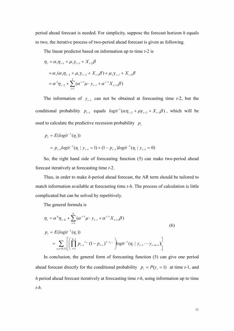
11
period ahead forecast is needed. For simplicity, suppose the forecast horizon h equals
to two, the iterative process of two-period ahead forecast is given as following.
The linear predictor based on information up to time t-2 is
βµηαη 21111 y -tttt X++= −−
)(
y)y(
1
12
1
1
2
2
211321211
βαµαηα
βµβµηαα
-i-t
i
i
it
i
t
-tt-ttt
Xy
XX
−
=−
−−
−−−
+⋅+=
++++=
∑
The information of 1−ty can not be obtained at forecasting time t-2, but the
conditional probability 1−tp equals )y( 322
1 βµαη -ttt
- Xlogit ++ −− , which will be
used to calculate the predictive recession probability tp
))(( 1
tt ηlogitEp −=
)0()1()1( 1
1
11
1
1 =−+== −−
−−−
− tttttt y|ηlogitpy|ηlogitp
So, the right hand side of forecasting function (5) can make two-period ahead
forecast iteratively at forecasting time t-2.
Thus, in order to make h-period ahead forecast, the AR term should be tailored to
match information available at forecasting time t-h. The process of calculation is little
complicated but can be solved by repetitively.
The general formula is
)( 1
1h
1
1
h
h βαµαηαη -i-t
i
i
it
i
tt Xy −
=−
−− +⋅+= ∑
∑ ∏∈
+−−−
−
=
−−−
−
−=
=
−
)1,0(y
1h1
11
1
1
ii
1
t
ii )()1(
))((
ttt
h
i
y
t
y
t
tt
yy|ηlogitpp
ηlogitEp
t-tL
In conclusion, the general form of forecasting function (5) can give one period
ahead forecast directly for the conditional probability )1( == tt yPp at time t-1, and
h period ahead forecast iteratively at forecasting time t-h, using information up to time
t-h.
(6)
12
2.2.5 Model selection criteria
Model comparison can be carried out by evaluating the goodness-of-fit measures,
one of which is Schwarz-Bayesian information criterion, BIC (Schwarz, 1978),
2
)(L
TlogK-logBIC +=
Where logL is the log-likelihood function, K is the number of estimated
parameters, and T is the number of observations. The model is fitting better when the
value of this statistic is declining.
A facilitated measure of evaluating the performance of predictive model is the
percentage of correct prediction. The goodness-of-fit of model to data can be checked
visually by a cross table as table 4.
Finally, standard errors and p-values of estimated parameters are also considered
when checking the goodness-of-fit of specification models.
3 Results
In this part, the performance of AR logit model (3) is checked by forecasting
business cycle recession periods for U.S. and Sweden respectively. The predictive
power of AR logit model can be examined by corresponding figures and cross tables.
We are mainly interested in out-of-sample performance of the model, but it is also
very helpful to check its in-sample forecasting first in choosing the explanatory
variables and corresponding lags.
3.1 Model selection and in-sample results
3.1.1 Empirical analysis to U.S.
The in-sample performance of AR logit model can be evaluated by the goodness-
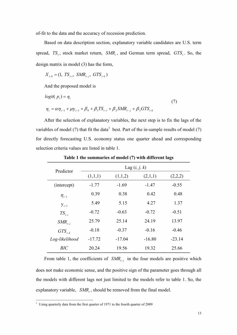
13
of-fit to the data and the accuracy of recession prediction.
Based on data description section, explanatory variable candidates are U.S. term
spread, tTS , stock market return, tSMR , and German term spread, tGTS . So, the
design matrix in model (3) has the form,
),,,1( k-tj-ti-th-t GTS SMRTS X =
And the proposed model is
tt ηp logit =)(
k-tjtitttt GTSSMRTSη 321011 y ββββµαη +++++= −−−−
After the selection of explanatory variables, the next step is to fix the lags of the
variables of model (7) that fit the data1 best. Part of the in-sample results of model (7)
for directly forecasting U.S. economy status one quarter ahead and corresponding
selection criteria values are listed in table 1.
Table 1 the summaries of model (7) with different lags
Lag (i, j, k) Predictor
(1,1,1) (1,1,2) (2,1,1) (2,2,2)
(intercept) -1.77 -1.69 -1.47 -0.55
1−tη 0.39 0.38 0.42 0.48
1y −t 5.49 5.15 4.27 1.37
i-tTS -0.72 -0.63 -0.72 -0.51
j-tSMR 25.79 25.14 24.19 13.97
k-tGTS -0.18 -0.37 -0.16 -0.46
Log-likelihood -17.72 -17.04 -16.80 -23.14
BIC 20.24 19.56 19.32 25.66
From table 1, the coefficients of j-tSMR in the four models are positive which
does not make economic sense, and the positive sign of the parameter goes through all
the models with different lags not just limited to the models refer to table 1. So, the
explanatory variable, tSMR , should be removed from the final model.
1 Using quarterly data from the first quarter of 1971 to the fourth quarter of 2009
(7)
14
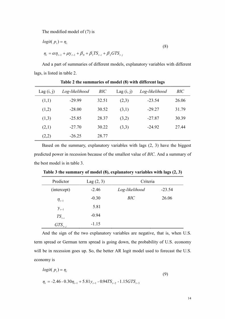
The modified model of (7) is
tt)( ηp logit =
j-titttt GTSTSη 21011 y βββµαη ++++= −−−
And a part of summaries of different models, explanatory variables with different
lags, is listed in table 2.
Table 2 the summaries of model (8) with different lags
Lag (i, j) Log-likelihood BIC Lag (i, j) Log-likelihood BIC
(1,1) -29.99 32.51 (2,3) -23.54 26.06
(1,2) -28.00 30.52 (3,1) -29.27 31.79
(1,3) -25.85 28.37 (3,2) -27.87 30.39
(2,1) -27.70 30.22 (3,3) -24.92 27.44
(2,2) -26.25 28.77
Based on the summary, explanatory variables with lags (2, 3) have the biggest
predicted power in recession because of the smallest value of BIC. And a summary of
the best model is in table 3.
Table 3 the summary of model (8), explanatory variables with lags (2, 3)
Predictor Lag (2, 3) Criteria
(intercept) -2.46 Log-likelihood -23.54
1−tη -0.30 BIC 26.06
1y −t 5.81
i-tTS -0.94
j-tGTS -1.15
And the sign of the two explanatory variables are negative, that is, when U.S.
term spread or German term spread is going down, the probability of U.S. economy
will be in recession goes up. So, the better AR logit model used to forecast the U.S.
economy is
tt ηp logit =)(
3211 15.194.081.530.046.2 −−−− += ttttt GTS-TS-yη--η
(8)
(9)
15
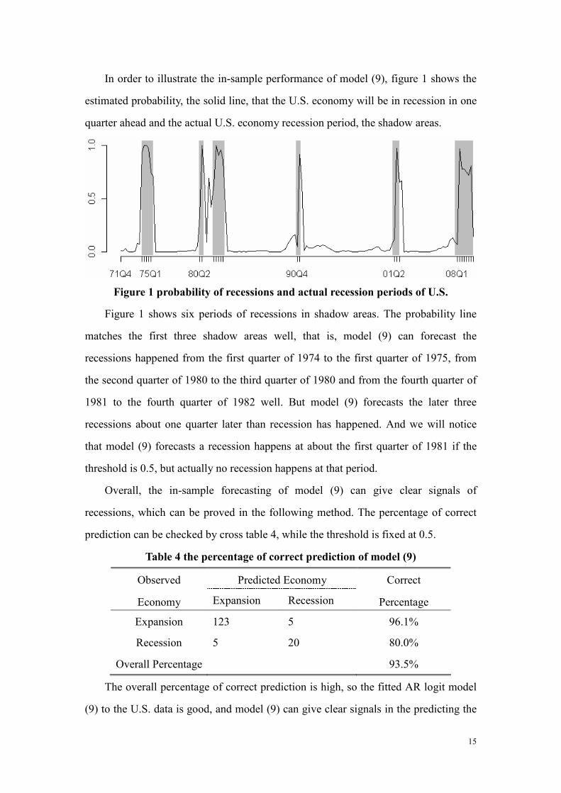
In order to illustrate the in-sample performance of model (9), figure 1 shows the
estimated probability, the solid line, that the U.S. economy will be in recession in one
quarter ahead and the actual U.S. economy recession period, the shadow areas.
Figure 1 probability of recessions and actual recession periods of U.S.
Figure 1 shows six periods of recessions in shadow areas. The probability line
matches the first three shadow areas well, that is, model (9) can forecast the
recessions happened from the first quarter of 1974 to the first quarter of 1975, from
the second quarter of 1980 to the third quarter of 1980 and from the fourth quarter of
1981 to the fourth quarter of 1982 well. But model (9) forecasts the later three
recessions about one quarter later than recession has happened. And we will notice
that model (9) forecasts a recession happens at about the first quarter of 1981 if the
threshold is 0.5, but actually no recession happens at that period.
Overall, the in-sample forecasting of model (9) can give clear signals of
recessions, which can be proved in the following method. The percentage of correct
prediction can be checked by cross table 4, while the threshold is fixed at 0.5.
Table 4 the percentage of correct prediction of model (9)
Predicted Economy Observed
Economy Expansion Recession
Correct
Percentage
Expansion 123 5 96.1%
Recession 5 20 80.0%
Overall Percentage 93.5%
The overall percentage of correct prediction is high, so the fitted AR logit model
(9) to the U.S. data is good, and model (9) can give clear signals in the predicting the
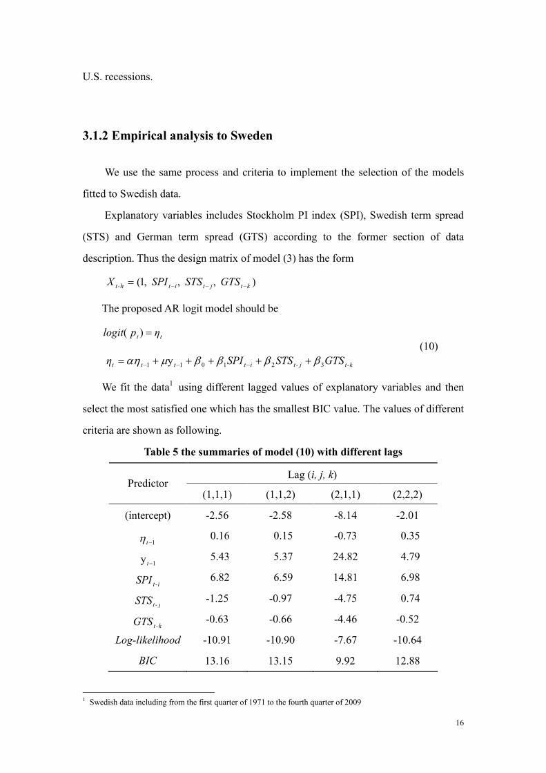
16
U.S. recessions.
3.1.2 Empirical analysis to Sweden
We use the same process and criteria to implement the selection of the models
fitted to Swedish data.
Explanatory variables includes Stockholm PI index (SPI), Swedish term spread
(STS) and German term spread (GTS) according to the former section of data
description. Thus the design matrix of model (3) has the form
),,,1( ktjtith-t GTS STS SPIX −−−=
The proposed AR logit model should be
tt ηp logit =)(
k-tj-titttt GTSSTSSPIη 321011 y ββββµαη +++++= −−−
We fit the data1 using different lagged values of explanatory variables and then
select the most satisfied one which has the smallest BIC value. The values of different
criteria are shown as following.
Table 5 the summaries of model (10) with different lags
Lag (i, j, k) Predictor
(1,1,1) (1,1,2) (2,1,1) (2,2,2)
(intercept) -2.56 -2.58 -8.14 -2.01
1−tη 0.16 0.15 -0.73 0.35
1y −t 5.43 5.37 24.82 4.79
i-tSPI 6.82 6.59 14.81 6.98
j-tSTS -1.25 -0.97 -4.75 0.74
k-tGTS -0.63 -0.66 -4.46 -0.52
Log-likelihood -10.91 -10.90 -7.67 -10.64
BIC 13.16 13.15 9.92 12.88
1 Swedish data including from the first quarter of 1971 to the fourth quarter of 2009
(10)
17
From the above results, the sign of coefficient of Stockholm PI index is positive
which does not make economic sense. Meanwhile the coefficient is a little larger than
expected. So, Stockholm PI index can not be used as explanatory variable and deleted
from design matrix.
And the new proposed AR logit model is
tt ηp logit =)(
j-ti-tttt GTSSTSη 21011 y βββµαη ++++= −−
The next step is to decide the lagged values of explanatory variables, STS and
GTS. Since when employed long lags, the degree of freedom will be sacrificed
correspondingly, we only compare the models that explanatory variables with lags up
to four for simplicity.
After simple calculation, we find that model with lagged values ),( 43 -t-t GTS STS
has the smaller BIC value and the signs of explanatory variables’ coefficients make
sense. And a good result is that the BIC is not declining when lags increase, that is to
say, the influence power of STS and GTS on the current Swedish economy status is
increasing within one year and then reducing as time passes.
The summary of the final model is shown as below.
Table 6 the summary of model (11), explanatory variables with lags (3, 4)
Predictor Lag (3, 4) Criteria
(intercept) -2.40 Log-likelihood -10.43
1−tη -0.18 BIC 12.67
1y −t 5.54
itSTS − -1.29
j-tGTS -0.63
Then the final model is
tt ηp logit =)(
431 63.029.154.518.040.2 -ttt1-tt GTSSTSy −−+−−= −−ηη
To illustrate the in-sample performance of model (12), figure 2 shows the
(11)
(12)
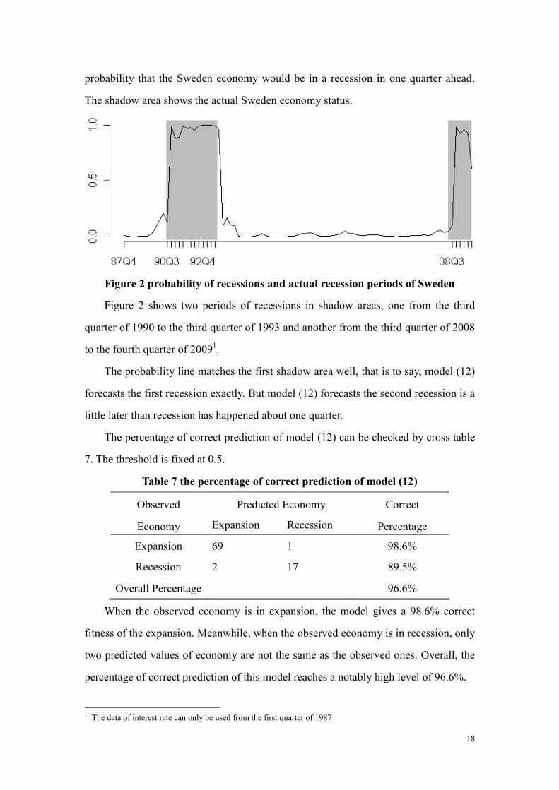
18
probability that the Sweden economy would be in a recession in one quarter ahead.
The shadow area shows the actual Sweden economy status.
Figure 2 probability of recessions and actual recession periods of Sweden
Figure 2 shows two periods of recessions in shadow areas, one from the third
quarter of 1990 to the third quarter of 1993 and another from the third quarter of 2008
to the fourth quarter of 20091.
The probability line matches the first shadow area well, that is to say, model (12)
forecasts the first recession exactly. But model (12) forecasts the second recession is a
little later than recession has happened about one quarter.
The percentage of correct prediction of model (12) can be checked by cross table
7. The threshold is fixed at 0.5.
Table 7 the percentage of correct prediction of model (12)
Predicted Economy Observed
Economy Expansion Recession
Correct
Percentage
Expansion 69 1 98.6%
Recession 2 17 89.5%
Overall Percentage 96.6%
When the observed economy is in expansion, the model gives a 98.6% correct
fitness of the expansion. Meanwhile, when the observed economy is in recession, only
two predicted values of economy are not the same as the observed ones. Overall, the
percentage of correct prediction of this model reaches a notably high level of 96.6%.
1 The data of interest rate can only be used from the first quarter of 1987
19
3.2 Out-of-sample results
Out-of-sample performance of the specified models will be mainly concerned,
and this section will check the predicted power of the models specified in the previous
section.
3.2.1 Out-of-sample results of U.S.
Based on previous section, the model (9) can predict well in one quarter ahead
in-sample U.S. recession forecasts. So, consider using the same model, explanatory
variables with same lags, to check the out-of-sample performance of AR logit model
in U.S. recession forecasting.
tt)( ηp logit =
3221011 y -ttttt GTSTSη βββµαη ++++= −−−
Because forecast horizon is two, model (13) can make one quarter ahead and two
quarters ahead forecasts.
Using data dated before forecasting quarter to estimate the parameters of model
(13), and the out-of-sample performance of model (13) one quarter ahead forecast is
shown as figure 3.
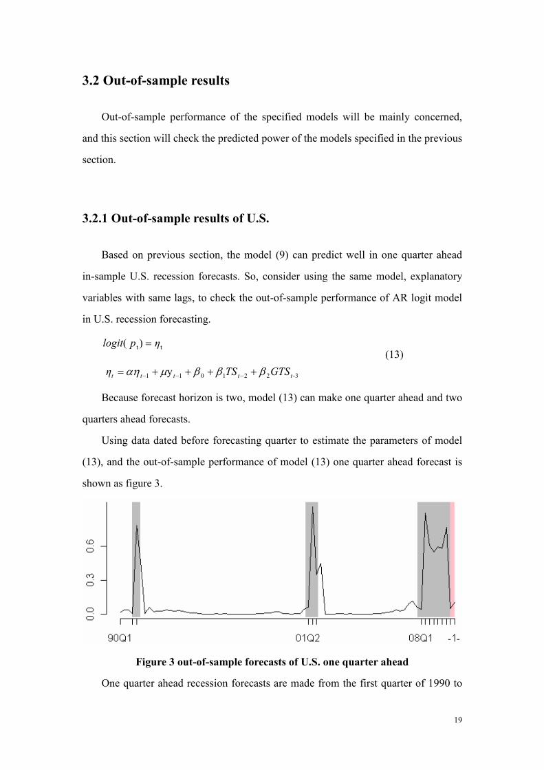
Figure 3 out-of-sample forecasts of U.S. one quarter ahead
One quarter ahead recession forecasts are made from the first quarter of 1990 to
(13)
20
the first quarter of 2010. Because the actual status the first quarter of 2010, in
recession or not, is not known, that means it is not included in the using data set, so
using pink background to make it different from the others.
From figure 3, there are three recession periods. The first recession period from
the fourth quarter of 1990 to first quarter of 1991 can be predicted well by the model.
But the later two recession period starting from the second quarter of 2001 and the
first quarter of 2008 can not be predicted exactly about one quarter late than the actual
starting quarters, respectively. And the economic recession predicted by model (13)
will end at the first quarter of 2010.
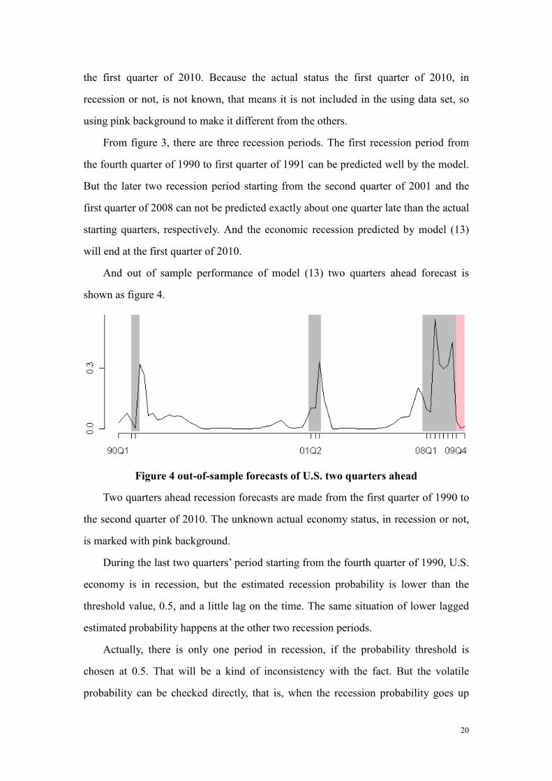
And out of sample performance of model (13) two quarters ahead forecast is
shown as figure 4.
Figure 4 out-of-sample forecasts of U.S. two quarters ahead
Two quarters ahead recession forecasts are made from the first quarter of 1990 to
the second quarter of 2010. The unknown actual economy status, in recession or not,
is marked with pink background.
During the last two quarters’ period starting from the fourth quarter of 1990, U.S.
economy is in recession, but the estimated recession probability is lower than the
threshold value, 0.5, and a little lag on the time. The same situation of lower lagged
estimated probability happens at the other two recession periods.
Actually, there is only one period in recession, if the probability threshold is
chosen at 0.5. That will be a kind of inconsistency with the fact. But the volatile
probability can be checked directly, that is, when the recession probability goes up
21
enough, economy recession happens in near periods. So, alternative choice is decrease
the threshold to 0.3, and the prediction power of the model has been changed higher.
Figure 4 also shows that the recession staring from the first quarter of 2008 will
end at the first quarter of 2010 finally.
3.2.2 Out-of-sample results of Sweden
Based on model (12), consider using following model to check the out-of-sample
performance of AR logit model in Sweden recession forecasting.
tt ηp logit =)(
4231011 y -t-tttt GTSSTSη βββµαη ++++= −−
Model (14) can make one quarter ahead up to three quarters ahead forecasts due
to its forecast horizon is three. We still use data dated before forecasting quarter to
estimate the parameters of model (14), and then make the out-of-sample forecast.
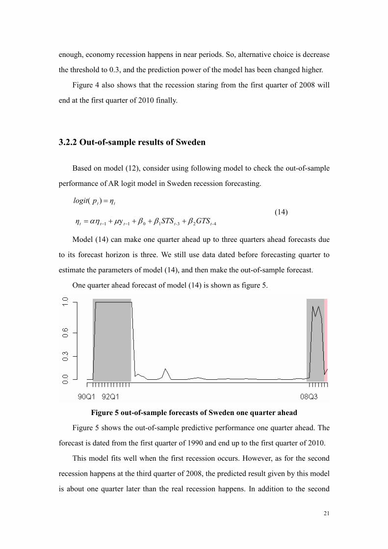
One quarter ahead forecast of model (14) is shown as figure 5.
Figure 5 out-of-sample forecasts of Sweden one quarter ahead
Figure 5 shows the out-of-sample predictive performance one quarter ahead. The
forecast is dated from the first quarter of 1990 and end up to the first quarter of 2010.
This model fits well when the first recession occurs. However, as for the second
recession happens at the third quarter of 2008, the predicted result given by this model
is about one quarter later than the real recession happens. In addition to the second
(14)
22
recession forecasting, the model matches well with the real data.
Since the status of economy at the first quarter of 2010 is unknown in the data set,
we use pink highlight to distinguish this period from others. Model (14) predicts that
the recession starting from the third quarter of 2008 will end at the first quarter of
2010.
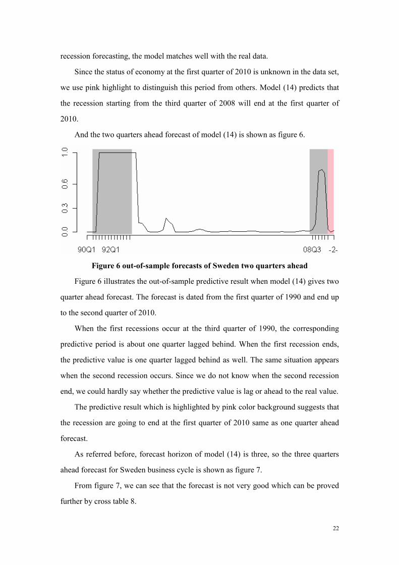
And the two quarters ahead forecast of model (14) is shown as figure 6.
Figure 6 out-of-sample forecasts of Sweden two quarters ahead
Figure 6 illustrates the out-of-sample predictive result when model (14) gives two
quarter ahead forecast. The forecast is dated from the first quarter of 1990 and end up
to the second quarter of 2010.
When the first recessions occur at the third quarter of 1990, the corresponding
predictive period is about one quarter lagged behind. When the first recession ends,
the predictive value is one quarter lagged behind as well. The same situation appears
when the second recession occurs. Since we do not know when the second recession
end, we could hardly say whether the predictive value is lag or ahead to the real value.
The predictive result which is highlighted by pink color background suggests that
the recession are going to end at the first quarter of 2010 same as one quarter ahead
forecast.
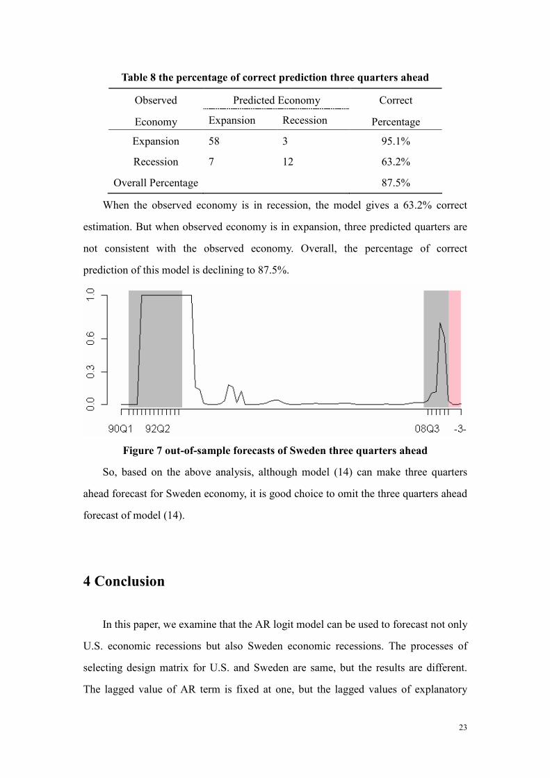
As referred before, forecast horizon of model (14) is three, so the three quarters
ahead forecast for Sweden business cycle is shown as figure 7.
From figure 7, we can see that the forecast is not very good which can be proved
further by cross table 8.
23
Table 8 the percentage of correct prediction three quarters ahead
Predicted Economy Observed
Economy Expansion Recession
Correct
Percentage
Expansion 58 3 95.1%
Recession 7 12 63.2%
Overall Percentage 87.5%
When the observed economy is in recession, the model gives a 63.2% correct
estimation. But when observed economy is in expansion, three predicted quarters are
not consistent with the observed economy. Overall, the percentage of correct
prediction of this model is declining to 87.5%.
Figure 7 out-of-sample forecasts of Sweden three quarters ahead
So, based on the above analysis, although model (14) can make three quarters
ahead forecast for Sweden economy, it is good choice to omit the three quarters ahead
forecast of model (14).
4 Conclusion
In this paper, we examine that the AR logit model can be used to forecast not only
U.S. economic recessions but also Sweden economic recessions. The processes of
selecting design matrix for U.S. and Sweden are same, but the results are different.
The lagged value of AR term is fixed at one, but the lagged values of explanatory
24
variables are flexible. Generally, the determination of the lagged values of
explanatory variables is through the BIC value of each model. After selecting the best
fitted model, we are more concern about the in-sample and out-of-sample forecasting
performance. The in-sample forecasting of U.S. with one quarter ahead shows a good
fitness of the model. Specifically, this model gives an overall 93.5% correction of
prediction. Thus, we can believe that the model will also suggest a good result for
out-of-sample forecasting. The in-sample forecasting performance of AR logit model
when applying it to Sweden shows an overall 96.6% correction of prediction. This
result indicates that the AR logit model is applicable in Sweden, what’s more, the
percentage correction of prediction even better than U.S. Thus, we can conclude that
the AR logit model is quite suitable when modeling the economy recession in
Sweden.
After comparing the in-sample forecasting performance of AR logit model, the
out-of-sample forecasting is more concerned when applying the model in practice.
Since the forecast horizon in U.S. model is two, we can implement the out-of-sample
forecasting up to two quarters ahead. We can get the forecasting result with one
quarter ahead directly, but when the step of forecasting is larger than one, we use
iterative method to get the forecasting results. Generally, the results of out-of-sample
forecasting are not as good as the ones of in-sample forecasting. To get a better visual
figure, we must limit the threshold to smaller value than 0.5 sometimes. Both the
forecasting results with one quarter ahead and two quarters ahead show a small
probability of recession which indicates the economy in U.S. will recover from a deep
recession. In other words, the economy in U.S. will experience an expansion at least
until second quarter in 2010. Since the forecast horizon in Sweden model is three, we
can implement the out-of-sample forecasting up to three quarters ahead. The
forecasting with one quarter ahead shows a better performance than the others.
Nevertheless, all these forecasting results show a small probability of recession at the
starting quarter of 2010 which means that the economy in Sweden will experience an
expansion at least up to the third quarter in 2010.
Although the AR logit model can be considered as a powerful tool to model and
25
predict economic recessions, we can observe from the figures that the predicted
recessions mostly occur later than the real ones. This phenomenon partly can be
explained as the lag effect of models. Since all the models we proposed include an AR
term, it makes sense when we observe the predicted results react later than the real
ones. Besides, it maybe interest to add more explanatory variables to improve the
performance of AR logit model or consider applying the AR logit model to describe
the economy recession in other homogeneous countries e.g. EEC is another possible
way for further study.
26
References
[1] Bodie Z., Kane A. & Marcus A. J., 2004. Investments. 6th ed. U.S.:
McGraw-Hill/Irwin.
[2] Chauvet M. & Potter S., 2005. Forecasting Recessions Using the Yield Curve.
Journal of Forecasting, 24(2), pp.77-103.
[3] Estrella A. & Mishkin F. S., 1998. Predicting U.S. Recessions: Financial Variables
as Leading Indicators. The Review of Economics and Statistics, 80(1), pp.45-61.
[4] Hamberg U. & Verständig D., 2009. Applying Logistic Regression Models on
Business Cycle Prediction. Unpublished master thesis, Stockholm School of
Economics.
[5] Kauppi H. & Saikkonen P., 2005. Predicting U.S. Recessions with Dynamic
Binary Response Models. Helsinki Center of Economic Research, Discussion
Paper No. 79.
[6] Moore.G.H, 1967. What is a Recession? The American Statistician, 21(4), pp.
16-190.
[7] Nyberg H., 2008. Testing an Autoregressive Structure in Binary Time Series
Models. Helsinki Center of Economic Research, Discussion Paper No. 243.
[8] Nyberg H., 2009. A Bivariate Autoregressive Probit Model: Predicting U.S.
Business Cycle and Growth Rate Cycle Recessions. Helsinki Center of Economic
Research, Discussion Paper No. 272.
[9] Omori Y., 2003. Discrete Duration Model Having Autoregressive Random Effects
with Application to Japanese Diffusion Index. Journal of the Japan statistical
society, 33(1), pp.1-22.
[10] Schwarz G., 1978. Estimating the Dimension of a Model. The Annals of Statistics,
6(2), pp.461-464.
[11] Startz R., 2006. Binomial Autoregressive Moving Average Models with an
Application to U.S. Recessions. Center for Statistics in the Social Sciences
University of Washington, Working Paper No. 56.