instantaneous frequency estimation based on time-varying auto regressive model and wax-kailath...

G. Ravi Shankar Reddy & Rameshwar Rao

Signal Processing : An International Journal (SPIJ), Volume (8) : Issue (4) : 2014 43

Instantaneous Frequency Estimation Based On Time-Varying Auto Regressive Model And WAX-Kailath Algorithm

G. Ravi Shankar Reddy [email protected]

Associate Professor, ECE Department, CVR college of Engineering, Hyderabad-85, India.

Rameshwar Rao [email protected] Vice- Chancellor, JNT UH, Hyderabad-85, India.

Abstract

Time-varying autoregressive (TVAR) model is used for modeling non stationary signals, Instantaneous frequency (IF) and time-varying power spectral density are then extracted from the TVAR parameters. TVAR based Instantaneous frequency (IF) estimation has been shown to perform very well in realistic scenario when IF variation is quick, non-linear and has short data record. In TVAR modeling approach, the time-varying parameters are expanded as linear combinations of a set of basis functions .In this article, time poly nominal is chosen as basis function. Non stationary signal IF is estimated by calculating the angles of the roots (poles) of the time-varying autoregressive polynomial at every sample instant. We propose modified covariance method that utilizes both the time varying forward and backward linear predictors for estimating the time-varying parameters and then IF estimate. It is shown that performance of proposed modified covariance method is superior than existing covariance method which uses only forward linear predictor for estimating the time-varying parameters. The IF evaluation based on TVAR modeling requires efficient estimation of the time-varying coefficients by solving a set of linear equations referred as the general covariance equations. When covariance matrix is of high order, usual approach such as Gaussian elimination or direct matrix inversion is computationally incompetent for solving such a structure of equations. We apply recursive algorithm to competently invert the covariance matrix, by means of Wax-Kailath algorithm which exploits the block-Toeplitz arrangement of the covariance matrix for its recursive inversion, which is the central part of this article. The order determination of TVAR model is addressed by means of the maximum likelihood estimation (MLE) algorithm. Keywords: Basis Functions, Instantaneous Frequency Estimation, Maximum Likelihood Estimation, Time-Varying Autoregressive Model, Wax-kailath Algorithm.

1. INTRODUCTION Non-Stationary signals are modeled using time-varying autoregressive (TVAR) model, the time-varying frequency of a non-stationary signal is extracted from the time-varying parameters of the TVAR model. There are different methods in literature for estimating the IF of non stationary signals and they are generally classified as non-parametric and parametric methods. In non-parametric methods we do not require any priori information regarding the characteristics of a signal and several of these techniques are based on the time-frequency distribution (TFD) of the signal. In the methods based on TFD, the IF is predicted from the peak of the TFD or its first moment [1]. Two familiar



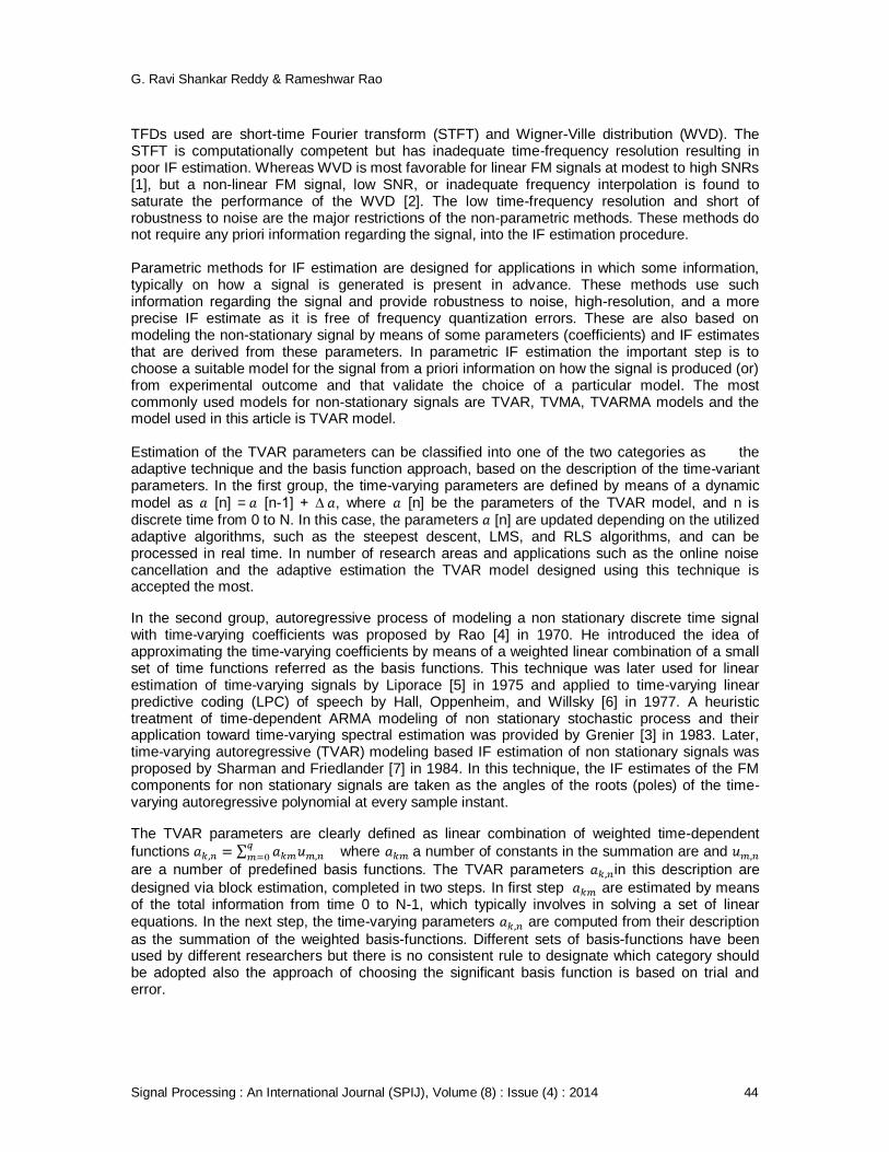
TFDs used are short-time Fourier transform (STFT) and Wigner-Ville distribution (WVD). The STFT is computationally competent but has inadequate time-frequency resolution resulting in poor IF estimation. Whereas WVD is most favorable for linear FM signals at modest to high SNRs [1], but a non-linear FM signal, low SNR, or inadequate frequency interpolation is found to saturate the performance of the WVD [2]. The low time-frequency resolution and short of robustness to noise are the major restrictions of the non-parametric methods. These methods do not require any priori information regarding the signal, into the IF estimation procedure. Parametric methods for IF estimation are designed for applications in which some information, typically on how a signal is generated is present in advance. These methods use such information regarding the signal and provide robustness to noise, high-resolution, and a more precise IF estimate as it is free of frequency quantization errors. These are also based on modeling the non-stationary signal by means of some parameters (coefficients) and IF estimates that are derived from these parameters. In parametric IF estimation the important step is to choose a suitable model for the signal from a priori information on how the signal is produced (or) from experimental outcome and that validate the choice of a particular model. The most commonly used models for non-stationary signals are TVAR, TVMA, TVARMA models and the model used in this article is TVAR model. Estimation of the TVAR parameters can be classified into one of the two categories as the adaptive technique and the basis function approach, based on the description of the time-variant parameters. In the first group, the time-varying parameters are defined by means of a dynamic model as [n] = [n-1] + ∆ , where [n] be the parameters of the TVAR model, and n is discrete time from 0 to N. In this case, the parameters [n] are updated depending on the utilized adaptive algorithms, such as the steepest descent, LMS, and RLS algorithms, and can be processed in real time. In number of research areas and applications such as the online noise cancellation and the adaptive estimation the TVAR model designed using this technique is accepted the most.

In the second group, autoregressive process of modeling a non stationary discrete time signal with time-varying coefficients was proposed by Rao [4] in 1970. He introduced the idea of approximating the time-varying coefficients by means of a weighted linear combination of a small set of time functions referred as the basis functions. This technique was later used for linear estimation of time-varying signals by Liporace [5] in 1975 and applied to time-varying linear predictive coding (LPC) of speech by Hall, Oppenheim, and Willsky [6] in 1977. A heuristic treatment of time-dependent ARMA modeling of non stationary stochastic process and their application toward time-varying spectral estimation was provided by Grenier [3] in 1983. Later, time-varying autoregressive (TVAR) modeling based IF estimation of non stationary signals was proposed by Sharman and Friedlander [7] in 1984. In this technique, the IF estimates of the FM components for non stationary signals are taken as the angles of the roots (poles) of the time-varying autoregressive polynomial at every sample instant.

The TVAR parameters are clearly defined as linear combination of weighted time-dependent

functions where a number of constants in the summation are and

are a number of predefined basis functions. The TVAR parameters in this description are

designed via block estimation, completed in two steps. In first step are estimated by means of the total information from time 0 to N-1, which typically involves in solving a set of linear equations. In the next step, the time-varying parameters are computed from their description

as the summation of the weighted basis-functions. Different sets of basis-functions have been used by different researchers but there is no consistent rule to designate which category should be adopted also the approach of choosing the significant basis function is based on trial and error.



The adaptive algorithms are able to track the slowly time-varying frequencies, but they are not able to track rapidly time-varying frequencies, and are also sensitive to the noise. The sensitivity to the noise can be reduced by increasing the forgetting factor or step size of adaptive algorithms, but at the cost of convergence rate of the adaptive algorithms and ability of tracking the parameter change. Still they were capable in tracking the frequency jump. Also the basis function technique is capable of tracking equally the fast (or) the slow time-varying frequencies. But the choice of the TVAR model order and the basis function is disputed since there is no fundamental theorem on how to choose them.

In this paper a new forward-backward prediction (modified covariance)approach based on basis functions for time-varying frequency estimation of the non stationary signal in a noisy environment is proposed. It is shown that our approach yields better accuracy than the existing covariance approach, which uses only the forward predictor.

The article is presented as follows. It explains the Time-varying Autoregressive modeling in section 2. In section 3 it explains the selection of basis function and TVAR model order determination by means of Maximum likelihood estimator. We briefly give details about the Wax-kailath algorithm to estimate the TVAR parameters in section 4. In section 5 it gives the steps to estimate IF based on TVAR model. The investigational results of estimating IF in noisy environment are presented in section 6.Concluding remarks are given in section7.

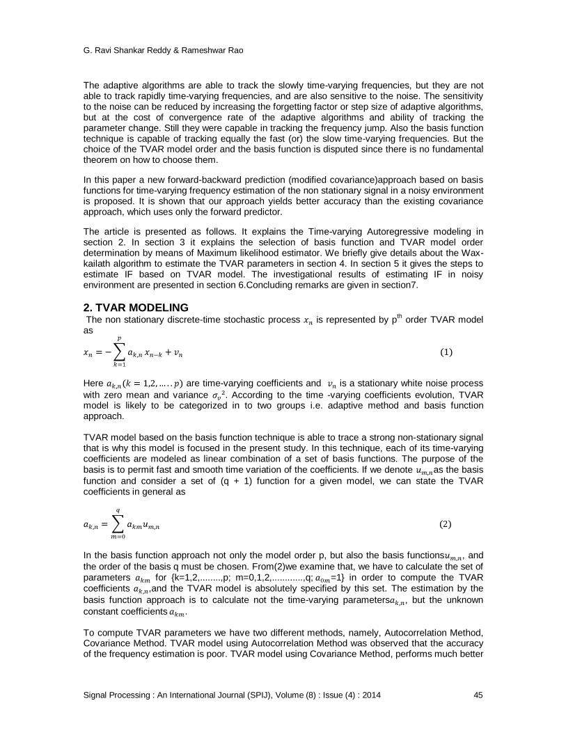
2. TVAR MODELING The non stationary discrete-time stochastic process is represented by p

th order TVAR model

as

Here are time-varying coefficients and is a stationary white noise process

with zero mean and variance According to the time -varying coefficients evolution, TVAR model is likely to be categorized in to two groups i.e. adaptive method and basis function approach. TVAR model based on the basis function technique is able to trace a strong non-stationary signal that is why this model is focused in the present study. In this technique, each of its time-varying coefficients are modeled as linear combination of a set of basis functions. The purpose of the basis is to permit fast and smooth time variation of the coefficients. If we denote as the basis

function and consider a set of (q + 1) function for a given model, we can state the TVAR coefficients in general as

In the basis function approach not only the model order p, but also the basis functions , and

the order of the basis q must be chosen. From(2)we examine that, we have to calculate the set of parameters for {k=1,2,........,p; m=0,1,2,............,q; =1} in order to compute the TVAR coefficients ,and the TVAR model is absolutely specified by this set. The estimation by the

basis function approach is to calculate not the time-varying parameters , but the unknown

constant coefficients . To compute TVAR parameters we have two different methods, namely, Autocorrelation Method, Covariance Method. TVAR model using Autocorrelation Method was observed that the accuracy of the frequency estimation is poor. TVAR model using Covariance Method, performs much better



than Autocorrelation method, was observed to have yielded a frequency estimate, which was about one-step delay of the true frequency. In addition ,by using TVAR model using Covariance Method, the frequency estimate at the time instant n=0,1,2,……..p-1 was unavailable, since the calculation must be delayed p steps before it could be started. In this article we propose a Modified Covariance method by applying a combination of a time varying forward and a backward linear estimators that results in no delay of the frequency estimate (i.e. frequency can be estimated from n=0,1,…..N-1. And the frequency estimate is also about the true frequency).In the case in which the model order was over determined, the performance of the proposed method in time-varying frequency estimation is much better than the Autocorrelation and Covariance methods. The non stationary signal is predicted using the TVAR parameters as shown below

2.1. Modified Covariance Method In order to compute TVAR parameters we propose modified Covariance method. The TVAR parameters are calculated by minimizing both, time varying forward and backward prediction errors. The above mentioned method is carried out by following below given steps. Let us assume data is available for 0,1,2.......N-1 time instants. Time varying forward linear prediction of can be defined as

And Time varying backward linear prediction of can be defined as

Time varying forward linear Prediction error is defined as

And Time varying backward linear prediction error is defined as

It was shown in Marple (1987), Manolakis et al. (2005) that the forward and backward linear prediction parameters for a stationary random process are simply complex conjugates. In the Non stationary case we assume



Time varying forward and Backward Mean Square Prediction Error

Since and are equal, the above equal can be written as

To minimize the above equation we perform derivative with respect to and equate to zero

i.e.

Equating above term to zero we get

Define the functions



Using the equations (15) and (16) the equation (14) can be rewritten as

The above equation represents a system of p(q+1) linear equations. The above system of linear equations can be efficiently represented in matrix form as follows. Define a column vector as follows

We can use the function (15) to find the following matrix for

The above matrix is of size pxp and all the different values for m and g resulting in (q+1)x(q+1) such matrices, by means of these matrices, we can now describe a block matrix as shown below,

The above Block matrix C has (q+1)x(q+1) elements and each element is a matrix of size pxp, which implies the Block matrix C of size p(q+1)x p(q+1). Now we describe a column vector as shown below

By using the definitions from (18)-(21) we can represent the system of linear equations in (17) in a compact matrix form as follows



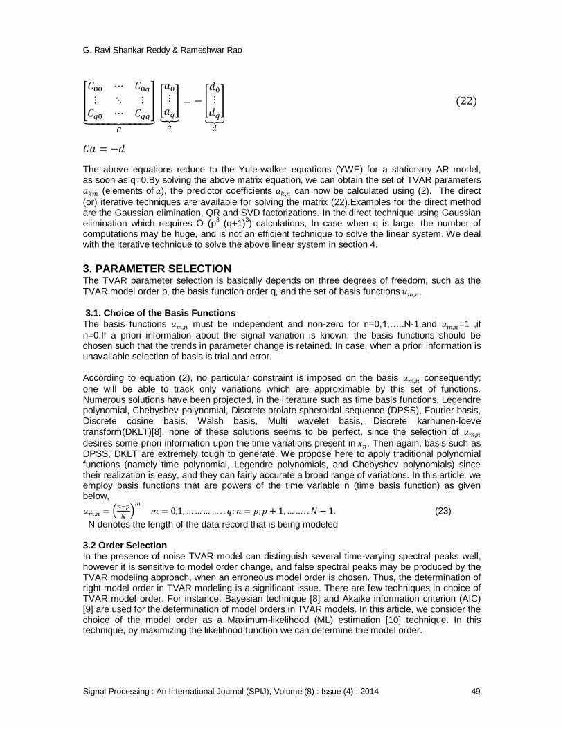
The above equations reduce to the Yule-walker equations (YWE) for a stationary AR model, as soon as q=0.By solving the above matrix equation, we can obtain the set of TVAR parameters

(elements of ), the predictor coefficients can now be calculated using (2). The direct

(or) iterative techniques are available for solving the matrix (22).Examples for the direct method are the Gaussian elimination, QR and SVD factorizations. In the direct technique using Gaussian elimination which requires O (p

3 (q+1)

3) calculations, In case when q is large, the number of

computations may be huge, and is not an efficient technique to solve the linear system. We deal with the iterative technique to solve the above linear system in section 4.

3. PARAMETER SELECTION The TVAR parameter selection is basically depends on three degrees of freedom, such as the TVAR model order p, the basis function order q, and the set of basis functions .

3.1. Choice of the Basis Functions

The basis functions must be independent and non-zero for n=0,1,…..N-1,and =1 ,if

n=0.If a priori information about the signal variation is known, the basis functions should be chosen such that the trends in parameter change is retained. In case, when a priori information is unavailable selection of basis is trial and error. According to equation (2), no particular constraint is imposed on the basis consequently;

one will be able to track only variations which are approximable by this set of functions. Numerous solutions have been projected, in the literature such as time basis functions, Legendre polynomial, Chebyshev polynomial, Discrete prolate spheroidal sequence (DPSS), Fourier basis, Discrete cosine basis, Walsh basis, Multi wavelet basis, Discrete karhunen-loeve transform(DKLT)[8], none of these solutions seems to be perfect, since the selection of

desires some priori information upon the time variations present in . Then again, basis such as DPSS, DKLT are extremely tough to generate. We propose here to apply traditional polynomial functions (namely time polynomial, Legendre polynomials, and Chebyshev polynomials) since their realization is easy, and they can fairly accurate a broad range of variations. In this article, we employ basis functions that are powers of the time variable n (time basis function) as given below,

(23)

N denotes the length of the data record that is being modeled 3.2 Order Selection In the presence of noise TVAR model can distinguish several time-varying spectral peaks well, however it is sensitive to model order change, and false spectral peaks may be produced by the TVAR modeling approach, when an erroneous model order is chosen. Thus, the determination of right model order in TVAR modeling is a significant issue. There are few techniques in choice of TVAR model order. For instance, Bayesian technique [8] and Akaike information criterion (AIC) [9] are used for the determination of model orders in TVAR models. In this article, we consider the choice of the model order as a Maximum-likelihood (ML) estimation [10] technique. In this technique, by maximizing the likelihood function we can determine the model order.



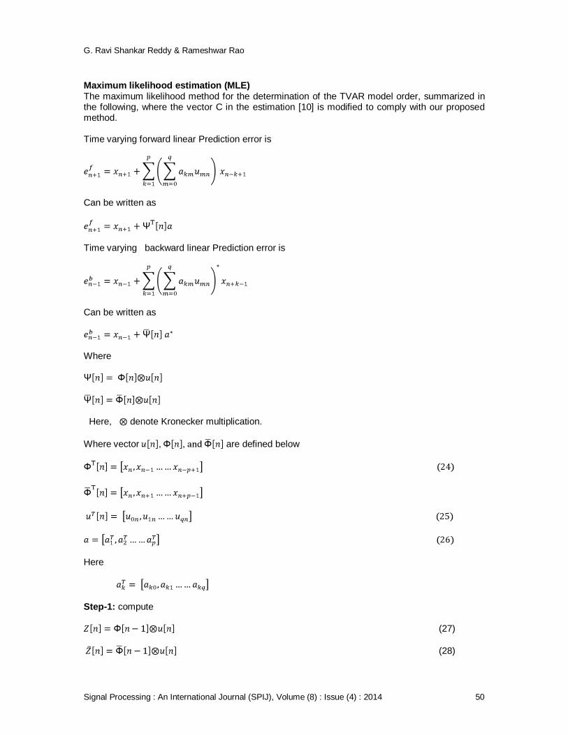
Maximum likelihood estimation (MLE) The maximum likelihood method for the determination of the TVAR model order, summarized in the following, where the vector C in the estimation [10] is modified to comply with our proposed method. Time varying forward linear Prediction error is

Can be written as

Time varying backward linear Prediction error is

Can be written as

Where

Here, denote Kronecker multiplication.

Where vector , , are defined below

Here

Step-1: compute

(27)

(28)



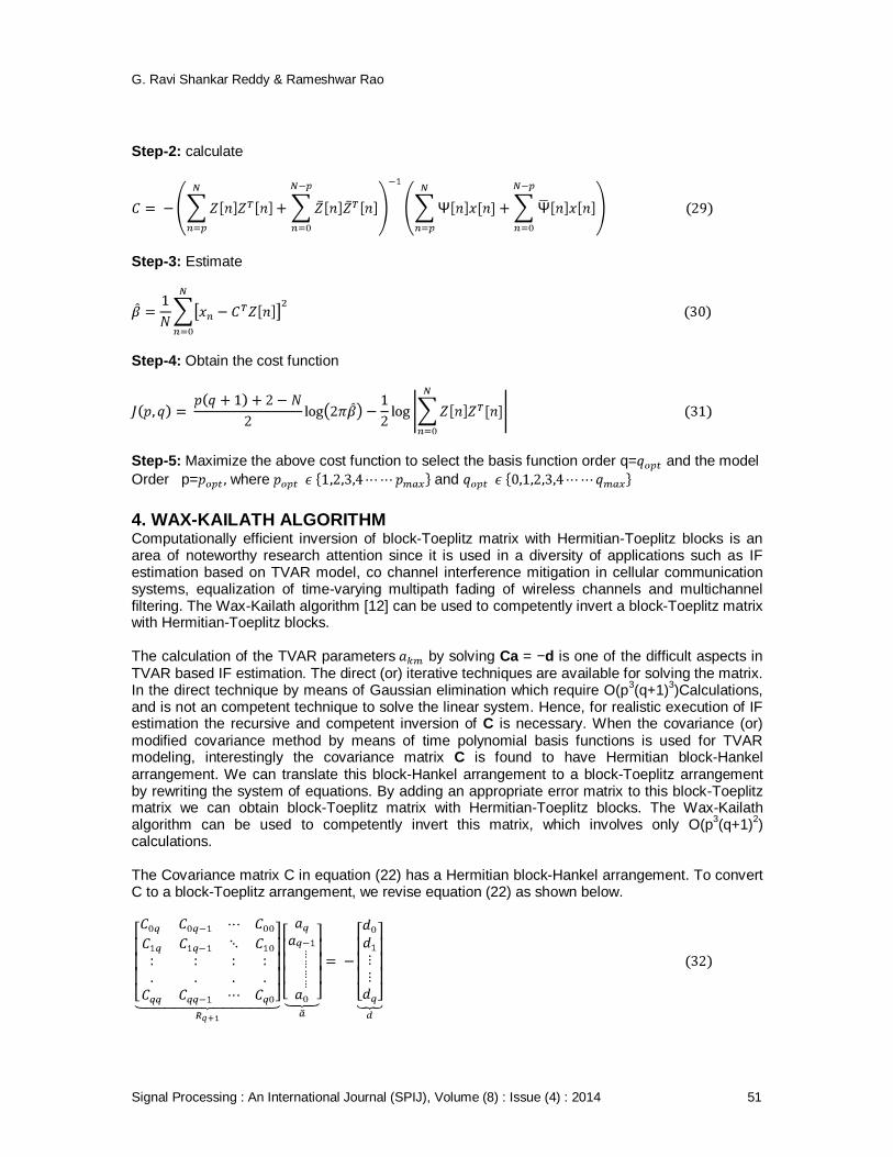
Step-2: calculate

Step-3: Estimate

Step-4: Obtain the cost function

Step-5: Maximize the above cost function to select the basis function order q= and the model

Order p= where and

4. WAX-KAILATH ALGORITHM Computationally efficient inversion of block-Toeplitz matrix with Hermitian-Toeplitz blocks is an area of noteworthy research attention since it is used in a diversity of applications such as IF estimation based on TVAR model, co channel interference mitigation in cellular communication systems, equalization of time-varying multipath fading of wireless channels and multichannel filtering. The Wax-Kailath algorithm [12] can be used to competently invert a block-Toeplitz matrix with Hermitian-Toeplitz blocks. The calculation of the TVAR parameters by solving Ca = −d is one of the difficult aspects in TVAR based IF estimation. The direct (or) iterative techniques are available for solving the matrix. In the direct technique by means of Gaussian elimination which require O(p

3(q+1)

3)Calculations,

and is not an competent technique to solve the linear system. Hence, for realistic execution of IF estimation the recursive and competent inversion of C is necessary. When the covariance (or) modified covariance method by means of time polynomial basis functions is used for TVAR modeling, interestingly the covariance matrix C is found to have Hermitian block-Hankel arrangement. We can translate this block-Hankel arrangement to a block-Toeplitz arrangement by rewriting the system of equations. By adding an appropriate error matrix to this block-Toeplitz matrix we can obtain block-Toeplitz matrix with Hermitian-Toeplitz blocks. The Wax-Kailath algorithm can be used to competently invert this matrix, which involves only O(p

3(q+1)

2)

calculations. The Covariance matrix C in equation (22) has a Hermitian block-Hankel arrangement. To convert C to a block-Toeplitz arrangement, we revise equation (22) as shown below.



The matrix in the above equation has block-Toeplitz structure with the individual blocks that

are Hermitian as well as being close to Toeplitz. Consequently, we add a suitable error matrix E to to get a block-Toeplitz matrix with Hermitian-Toeplitz blocks, which are then inverted

using Wax-Kailath Algorithm. By using m and g to index the blocks, the error matrix E can be formed as follows,

Here indicate the blocks in and is the equivalent Toeplitz block.

The Hermitian-Toeplitz blocks are formed as shown below,

Here, the function diag extract the i

th diagonal of the matrix unction mean, calculates

the mean of the ith diagonal, at last, the function toeplitz forms a Hermitian-Toeplitz matrix whose

foremost row elements equivalent to the mean of the diagonals. Using the above equation, we get and calculate to form the error matrix E.

The can be computed as

Where is a block-Toeplitz matrix with Hermitian-Toeplitz blocks of size p(q+1) x p(q+1) as

shown below

Here and for i=0,1,………..q are pxp matrices having Hermitian-Toeplitz arrangement as shown below

Now we describe a p(q+1) x p(q+1) exchange matrix as shown below,



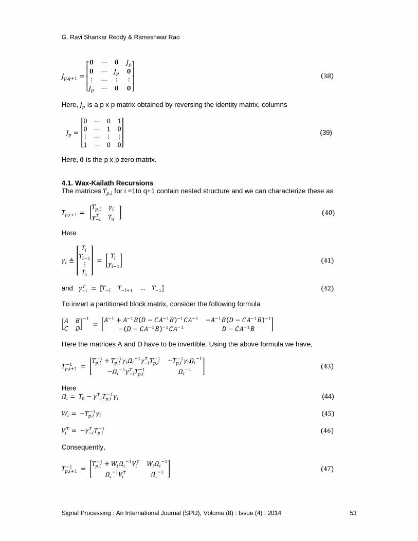
Here, is a p x p matrix obtained by reversing the identity matrix, columns

(39)

Here, is the p x p zero matrix. 4.1. Wax-Kailath Recursions The matrices for i =1to q+1 contain nested structure and we can characterize these as

Here

and To invert a partitioned block matrix, consider the following formula

Here the matrices A and D have to be invertible. Using the above formula we have,

Here

(44)

Consequently,



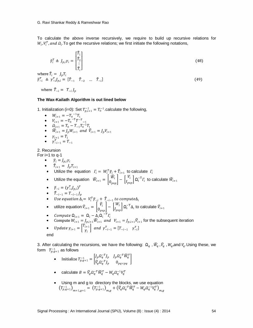
To calculate the above inverse recursively, we require to build up recursive relations for

.To get the recursive relations; we first initiate the following notations,

The Wax-Kailath Algorithm is out lined below

1. Initialization (i=0): Set .calculate the following,

2. Recursion For i=1 to q-1

Utilize the equation to calculate

Utilize the equation to calculate

utilize equation to calculate

for the subsequent iteration

end

3. After calculating the recursions, we have the following: , and .Using these, we

form as follows

calculate

Using m and g to directory the blocks, we use equation



To calculate the remaining blocks of the inverse matrix as follows, for m=1 to q for g=1 to q

end end The inverse of the block-Toeplitz matrix with Hermitian-Toeplitz blocks is obtained, by

means of Wax-Kailath algorithm; nevertheless, our interest is in computing the inverse of the block-Toeplitz covariance matrix with Hermitian blocks.From equation(36)we have

the inverse of the is , Can be computed by means of

Neumann series 4.2. Neumann Series Using the Wax-Kailath algorithm, we have obtained the inverse matrix of the block-Toepliitz matrix with Hermitian-Toeplitz blocks.However, our interest is in computing the inverse of

the block-Toeplitz covariance matrix with Hermitian blocks.

Using Neumann series can be written as

Where is the maximum absolute

eigenvalue of which also imply,

If the series converges, we are able to approximate by means of a finite number of

iterations and we can calculate the solution vector estimate. .Using this estimate we

can calculate an estimate of the solution of the linear system of equations C =-d as follows.

Where

Here, is the p x p identity matrix and is the p x p zero matrix. The elements of are the

elements in equation (2), subsequently calculate the TVAR parameters as follows



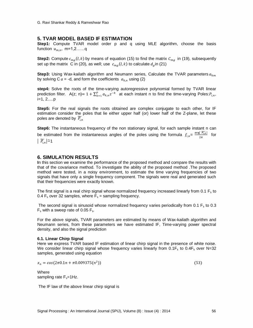
5. TVAR MODEL BASED IF ESTIMATION Step1: Compute TVAR model order p and q using MLE algorithm, choose the basis

function m=1,2……q

Step2: Compute by means of equation (15) to find the matrix in (19), subsequently

set up the matrix C in (20), as well; use to calculate in (21)

Step3: Using Wax-kailath algorithm and Neumann series, Calculate the TVAR parameters

by solving C = -d, and form the coefficients using (2)

step4: Solve the roots of the time-varying autoregressive polynomial formed by TVAR linear

prediction filter. A(z; n) at each instant n to find the time-varying Poles: ,

i=1, 2.....p Step5: For the real signals the roots obtained are complex conjugate to each other, for IF estimation consider the poles that lie either upper half (or) lower half of the Z-plane, let these

poles are denoted by

Step6: The instantaneous frequency of the non stationary signal, for each sample instant n can

be estimated from the instantaneous angles of the poles using the formula = for

1

6. SIMULATION RESULTS In this section we examine the performance of the proposed method and compare the results with that of the covariance method. To investigate the ability of the proposed method .The proposed method were tested, in a noisy environment, to estimate the time varying frequencies of two signals that have only a single frequency component. The signals were real and generated such that their frequencies were exactly known. The first signal is a real chirp signal whose normalized frequency increased linearly from 0.1 Fs to 0.4 Fs over 32 samples, where Fs = sampling frequency. The second signal is sinusoid whose normalized frequency varies periodically from 0.1 Fs to 0.3 Fs with a sweep rate of 0.05 Fs. For the above signals, TVAR parameters are estimated by means of Wax-kailath algorithm and Neumann series, from these parameters we have estimated IF, Time-varying power spectral density, and also the signal prediction 6.1. Linear Chirp Signal Here we express TVAR based IF estimation of linear chirp signal in the presence of white noise. We consider linear chirp signal whose frequency varies linearly from 0.1Fs to 0.4Fs over N=32 samples, generated using equation

Where sampling rate Fs=1Hz. The IF law of the above linear chirp signal is



The above signal is corrupted by means of a complex additive white Gaussian noise (AWGN) at SNR=20 dB. Using Maximum likely hood estimation algorithm we have calculated the TVAR model order p=2 and q=4.For the modified covariance technique the time polynomial basis function description is adapted as shown below

(55)

For p=2, q=4 and N=32, plot of the above basis function is revealed in Figure (1). The plot of the signal is revealed in Figure(2). A plot of the TVAR coefficients is shown in Figure(3).This

particular choice of basis functions results in a modified covariance matrix C that has a block-Hankel structure which can be exploited for computationally more efficient solutions. From Figure (4) we observe that the poles are close to the unit circle as expected. For every sample instant n, IF estimate of linear chirp signal is found by calculating the angles of the poles that lie in upper half of z plane, and then angles are divided by .The true IF & estimated IF of the linear chirp signal using covariance and modified covariance methods are revealed in Figure(5).We observe that the TVAR based technique has resulted in really nice IF estimation. The mean square error (MSE) among the true IF and estimated IF is calculated to be -46.7063 dB for covariance method and -57.3517dB for modified covariance method. We also observed that the performance of modified covariance method is superior than the covariance method.

The TVAR coefficients can also be used to predict the non stationary process by means

of equation(3).For the modified covariance technique, the parameters can be calculated only

for n=2,3,…….32.Consequently,the prediction is also available simply for this interval. The samples and in this simulation illustration are used as initial setting for the time-varying prediction error filter. The original data record in addition to the TVAR prediction are revealed in Figure(6).We observe that the TVAR model has effectively predicted .The average squared prediction error is calculated to be 0.1432. Although TVAR based IF estimation do not use a time frequency distribution (TFD) (or) the time-varying power spectrum, it is helpful to look at the TFD obtained from the TVAR model. The time-varying power spectral density is specified by

,P (f; n) = (56)

Where

are TVAR coefficients,

and is

(57)

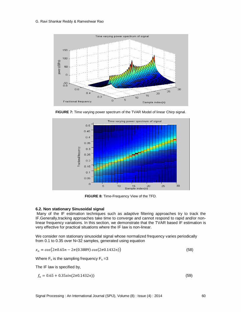
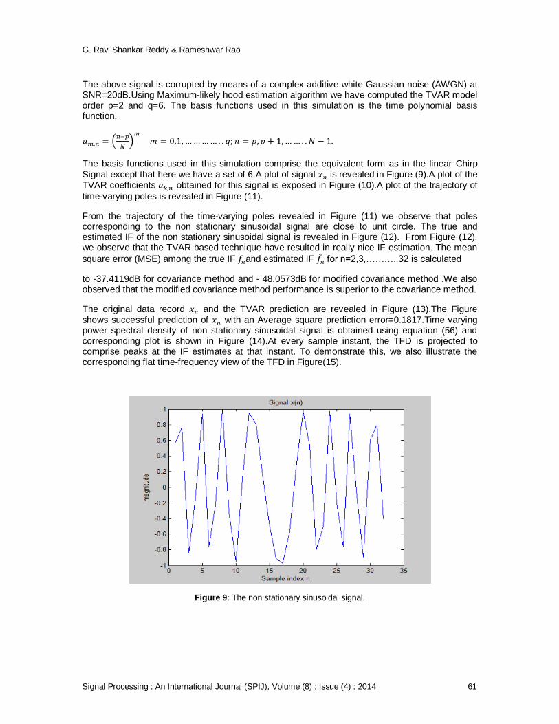
A plot of the time-frequency distribution for the TVAR model obtained in Figure (7).At every sample instant, the TFD is projected to comprise peaks at the IF estimates at that instant. To demonstrate this, we also illustrate the corresponding flat time-frequency view of the TFD in Figure(8).The time-frequency view of the TFD in Figure(8)clearly shows that the TFD peaks are consistent with the IF estimate and the true IF shown in Figure(5).The presented example shows that a TVAR based method works well for signals containing chirp signal whose frequency varies linearly



FIGURE 1: The Basis Function Set .

Figure 2: Linear Chirp signal.

FIGURE 3: Estimated TVAR Coefficients used for a Linear Chirp Signal.



FIGURE 4: Trajectory of Time-varying Poles used for a Linear Chirp Signal.

FIGURE 5: True and Estimated IF of Linear Chirp Signal.

FIGURE 6: Comparison of Original Data and TVAR Prediction for Linear Chirp signal.



FIGURE 7: Time varying power spectrum of the TVAR Model of linear Chirp signal.

FIGURE 8: Time-Frequency View of the TFD.

6.2. Non stationary Sinusoidal signal Many of the IF estimation techniques such as adaptive filtering approaches try to track the IF.Generally,tracking approaches take time to converge and cannot respond to rapid and/or non-linear frequency variations. In this section, we demonstrate that the TVAR based IF estimation is very effective for practical situations where the IF law is non-linear. We consider non stationary sinusoidal signal whose normalized frequency varies periodically from 0.1 to 0.35 over N=32 samples, generated using equation

(58)

Where Fs is the sampling frequency Fs =3

The IF law is specified by,

(59)



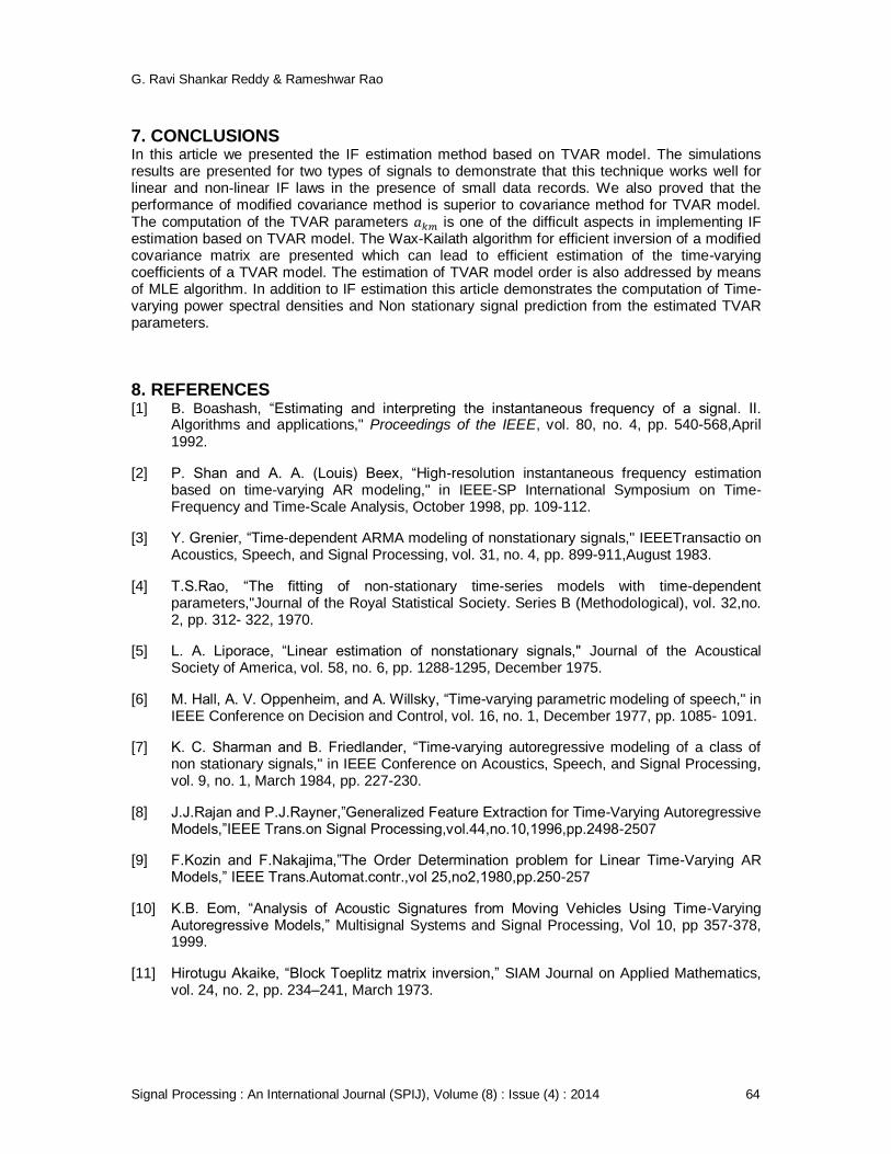
The above signal is corrupted by means of a complex additive white Gaussian noise (AWGN) at SNR=20dB.Using Maximum-likely hood estimation algorithm we have computed the TVAR model order p=2 and q=6. The basis functions used in this simulation is the time polynomial basis function.

The basis functions used in this simulation comprise the equivalent form as in the linear Chirp Signal except that here we have a set of 6.A plot of signal is revealed in Figure (9).A plot of the TVAR coefficients obtained for this signal is exposed in Figure (10).A plot of the trajectory of

time-varying poles is revealed in Figure (11).

From the trajectory of the time-varying poles revealed in Figure (11) we observe that poles corresponding to the non stationary sinusoidal signal are close to unit circle. The true and estimated IF of the non stationary sinusoidal signal is revealed in Figure (12). From Figure (12), we observe that the TVAR based technique have resulted in really nice IF estimation. The mean

square error (MSE) among the true IF and estimated IF for n=2,3,………..32 is calculated

to -37.4119dB for covariance method and - 48.0573dB for modified covariance method .We also observed that the modified covariance method performance is superior to the covariance method.

The original data record and the TVAR prediction are revealed in Figure (13).The Figure shows successful prediction of with an Average square prediction error=0.1817.Time varying power spectral density of non stationary sinusoidal signal is obtained using equation (56) and corresponding plot is shown in Figure (14).At every sample instant, the TFD is projected to comprise peaks at the IF estimates at that instant. To demonstrate this, we also illustrate the corresponding flat time-frequency view of the TFD in Figure(15).

Figure 9: The non stationary sinusoidal signal.



FIGURE 10: Estimated TVAR Coefficients for non stationary sinusoidal signal.

FIGURE 11: Trajectory of Time-varying poles used for non stationary sinusoidal signal.

FIGURE 12: True and Estimated IF of non stationary sinusoidal signal.



FIGURE 13: Comparison of TVAR prediction and original Data for non stationary sinusoidal signal

.

Figure 14: Time varying power spectrum of the TVAR model of non stationary Sinusoidal signal.

Figure 15: Time-Frequency View of the TFD of non stationary sinusoidal signal.



7. CONCLUSIONS In this article we presented the IF estimation method based on TVAR model. The simulations results are presented for two types of signals to demonstrate that this technique works well for linear and non-linear IF laws in the presence of small data records. We also proved that the performance of modified covariance method is superior to covariance method for TVAR model. The computation of the TVAR parameters is one of the difficult aspects in implementing IF estimation based on TVAR model. The Wax-Kailath algorithm for efficient inversion of a modified covariance matrix are presented which can lead to efficient estimation of the time-varying coefficients of a TVAR model. The estimation of TVAR model order is also addressed by means of MLE algorithm. In addition to IF estimation this article demonstrates the computation of Time-varying power spectral densities and Non stationary signal prediction from the estimated TVAR parameters.

8. REFERENCES [1] B. Boashash, “Estimating and interpreting the instantaneous frequency of a signal. II.

Algorithms and applications," Proceedings of the IEEE, vol. 80, no. 4, pp. 540-568,April 1992.

[2] P. Shan and A. A. (Louis) Beex, “High-resolution instantaneous frequency estimation based on time-varying AR modeling," in IEEE-SP International Symposium on Time-Frequency and Time-Scale Analysis, October 1998, pp. 109-112.

[3] Y. Grenier, “Time-dependent ARMA modeling of nonstationary signals," IEEETransactio on Acoustics, Speech, and Signal Processing, vol. 31, no. 4, pp. 899-911,August 1983.

[4] T.S.Rao, “The fitting of non-stationary time-series models with time-dependent parameters,"Journal of the Royal Statistical Society. Series B (Methodological), vol. 32,no. 2, pp. 312- 322, 1970.

[5] L. A. Liporace, “Linear estimation of nonstationary signals," Journal of the Acoustical Society of America, vol. 58, no. 6, pp. 1288-1295, December 1975.

[6] M. Hall, A. V. Oppenheim, and A. Willsky, “Time-varying parametric modeling of speech," in IEEE Conference on Decision and Control, vol. 16, no. 1, December 1977, pp. 1085- 1091.

[7] K. C. Sharman and B. Friedlander, “Time-varying autoregressive modeling of a class of non stationary signals," in IEEE Conference on Acoustics, Speech, and Signal Processing, vol. 9, no. 1, March 1984, pp. 227-230.

[8] J.J.Rajan and P.J.Rayner,”Generalized Feature Extraction for Time-Varying Autoregressive Models,”IEEE Trans.on Signal Processing,vol.44,no.10,1996,pp.2498-2507

[9] F.Kozin and F.Nakajima,”The Order Determination problem for Linear Time-Varying AR Models,” IEEE Trans.Automat.contr.,vol 25,no2,1980,pp.250-257

[10] K.B. Eom, “Analysis of Acoustic Signatures from Moving Vehicles Using Time-Varying Autoregressive Models,” Multisignal Systems and Signal Processing, Vol 10, pp 357-378, 1999.

[11] Hirotugu Akaike, “Block Toeplitz matrix inversion,” SIAM Journal on Applied Mathematics, vol. 24, no. 2, pp. 234–241, March 1973.



[12] Mati Wax and Thomas Kailath, “Efficient inversion of Toeplitz-block Toeplitz matrix,” IEEE Transactions on Acoustics Speech and Signal Processing, vol. ASSP-31, no. 5, pp. 1218–1747, October 1983.

[13] Carl D. Meyer, Matrix Analysis and Applied Linear Algebra, SIAM, Philadelphia, PA USA, 1 edition,2000.

[14] A. A. (Louis) Beex and P. Shan,”A time-varying Prony method for instantaneous frequency estimation at low SNR," in IEEE International Symposium on Circuits and Systems, vol. 3, May 1999, pp. 3-8.

[15] R.K.Pally, “Implementation of Instantaneous Frequency Estimation based on Time-Varying AR Modeling,”M.S.Thesis, Virginia Tech 2009.

[16] S. Mukhopadhyay, P. Sircar, “Parametric modeling of nonstationary signals: A unified approach, ” Signal Processing, Vol. 60, pp. 135-152, 1997.

[17] S.M. Kay, Modern Spectral Estimation: Theory and Application, Prentice-Hall, Englewood Cliffs, NJ,1988.

[18] M. Neidzwiecki, Identification of Time-varying Processes, John Wiley & Sons, Chicester, England, 2000.

[19] A.A Beex and P. Shan, “A time-varying prony method for instantaneous frequency estimation at low frequency,” Proceeding of the 1999 IEEE International Symphosium on Circuits and Systems, Vol 3, pp. 5-8, 1999.

[20] B. Barkat, Instantaneous frequency estimation of nonlinear frequency-modulated signals in the presence of multiplicative and additive noise," IEEE Transactions on Signal Processing, vol. 49, no. 10, pp. 2214-2222, October 2001.

[21] R. Charbonnier, M. Barlaud, G. Alengrin, and J. Menez, “Results on ARmodeling of nonstationary signals,” Elsevier Signal Processing, vol. 12, no.2, pp. 143-151, Mar. 1987.

[22] L. F. Chaparro and M. Boudaoud, “Recursive solution of the covariance equations for linear prediction,” J. Franklin Inst., vol. 320, pp. 161-167, Sept. 1985.

[23] F. Kozin, “Estimation and modeling of nonstationary time series,” in Proc.Symp. Appl Comput. Meth. Eng., vol. 1, pp. 603-612, Los Angeles, CA, 1977.

[24] P.Sircar, M.S. Syali, Complex AM signal model for non-stationary signals, Signal Processing

Vol.53,pp.35-45,1996

[25] P.Sircar, S. Sharma, Complex FM signal model for non-stationary signals, Signal Processing

Vol.53,pp.35-45,1996.

[26] A.Francos and M.Porat,”Non-stationary signal processing using time-frequency filter

banks with applications,”Signal Processing,vol.86,no 10,pp.3021-3030,October2006.

[27] M.Morf,B.Dickinson,T.Kailath,and A.Vieira,”Efficient solution of covariance equations for linear prediction,”IEEETransactionson Acoustics,Speech,and Signal Processing,vol.25,no.5,pp.429-433,October 1977

[28] A.T.Johansson and P.R.White,”Instantaneous frequency estimation at low signal-to-noise ratios using time-varying notch filters,”Signal Processing,vol.88,no.5,pp.1271-1288, May 2008



[29] A.E.Yagle,”A fast algorithm for Toeplitz-block-Toeplitz linear systems,” in IEEE International Conference on Acoustics,Speech and Signal Processing,vol.3,May 2001,pp.1929-1932.

[30] J.J.Rajan and P.J.W.Rayner,”Generalized Feature Extraction for Time-Varying Autoregressive Model,” IEEE Transactions on Signal Processing,Vol:44,No.10,pp 2498-2507,1996.

instantaneous frequency estimation based on time-varying auto regressive model and wax-kailath...

Education