Applying GIS data to model species distribution in response to climate change, using Maximum Entropy techniques. Nikhil K Advani Project outline Use of species presence records, along with environmental variables, to predict environmental suitability for a species, as a function of the given environmental variables. This process is done using GIS data (Arc GIS) along with niche based modeling (Maxent). Background Climate change is one of the most pressing concerns of this century, with severe biological impacts predicted (IPCC, 2007). Wild plants and animals are already responding to this process. Existing data on these responses principally concern changes in phenology, but observations of distributional change are also accumulating, including both elevational and latitudinal range shifts (Parmesan, 2006; Primack et. al., 2009). When these range shifts occur in non-migratory species they imply local changes in the ratio of population extinctions to population founding events, with extinctions dominating at receding range margins and colonizations at expanding range margins (Parmesan et. al., 1999; Pounds et. al., 1999; Parmesan, 2006). Different species, or populations within species, may show a variety of responses to climate change. Whilst some may actually thrive under new climate scenarios, others may decline and even go extinct. Thermal variables, such as the mean and variance of environmental temperature, have played a prominent role in defining fundamental niches (Lima et. al., 2007; Walther et. al., 2007). While the fundamental niche of a species may or may not be altered in response to regional warming, all species exhibit some genetic variation in thermal physiology, which should cause populations to respond differently over space and time. One approach to modeling distributional responses to climate change uses current ranges to create a 'climate envelope' for each species and assumes that these envelopes will be retained and can be projected onto future climate change scenarios. Using this approach, projections have been made that 20-40% of extant species will be exterminated by climate change in the near future (Thomas et. al., 2004). However, this approach may be a bit too simple, because observations show high variance in responses to ongoing climate warming, even among closely-related sympatric species (Parmesan et. al., 1999). Additionally, some climate models assume that species boundaries are determined by environmental factors statistically associated with occupancy, and that there exists little or no variation in thermal tolerance across the range of a species (Araujo & Luoto, 2007). Such models fail to account for biotic interactions between different species, barriers to dispersal or evolutionary adaptation. These are all legitimate concerns, however, at the very least these models can suggest that based on the species being studied, and the environmental variables tested, we can make certain projections on how the species may

1

respond to climate change. This could then aid us in developing conservation plans for such organisms in the face of climate change. Among the insects, butterflies are increasingly recognized as valuable environmental indicators, both for their rapid and sensitive responses to subtle habitat or climatic changes and as representatives for the diversity and responses of other arthropod wildlife. The limited dispersal of most butterflies, their larval host plant specialization and close-reliance on weather and climate make many of them sensitive to fine-scale changes. In consequence, climate is the most important predictor of butterfly species richness (Hawkins & Porter, 2003), temperature can be crucial in determining butterfly range limits (Crozier, 2004) and butterflies were among the first groups to show systematic range shifts matching predictions from current climate warming (Parmesan et al. 1999; Thomas et al. 2001). This study focuses on a well-studied butterfly, the Glanville Fritillary, Melitaea cinxia, a species that is well-known ecologically, behaviorally and genetically (Hanski, 1999). M. cinxia is distributed between approximately 35°N and 60°N in Europe and Asia (Lafranchis, 2004) and is also found in the Atlas mountains in Morocco. A niche based modeling technique, Maxent (see: http://www.cs.princeton.edu/~schapire/maxent/) is used in this study. A species’ fundamental niche describes the conditions (niche, in an ecological sense), and thus the potential area (in a geographic sense) within which a species can potentially survive, while its realized niche describes the niche (in an ecological sense)/area (in a geographic sense) that it actually occupies. A niche based model such as Maxent, thus represents an approximation of a species’ realized niche (Phillips et. al., 2006). Maxent essentially estimates a target probability distribution, by finding the probability distribution of maximum entropy, subject to constraints that represent incomplete information about the target distribution (Phillips et. al., 2006). Methods Known species localities: Data was gathered of know locations of M. cinxia, primarily consisting of actual collecting locations by myself, supplemented with 2 more sites (from collaborators). The data at hand are ideal for this kind of modeling, particularly since they represent the latitudinal and altitudinal range limits of the species (the low-elevation southern range limit: Catalunya, northern Spain, the northern range limit: Åland Islands, Finland and the elevational limit: the French Alps). GPS coordinates were gathered in different forms, and converted using an online application (http://boulter.com/gps/, see figure 1) to decimal degrees (WGS 84). Google Earth was used to find specific collecting localities (Figure 2) for which coordinates were not readily available. The GPS coordinates used in this study appear below:

2

Table 1: Known locations of M. cinxia Species Longitude Latitude M_Cinxia 19.78137 60.17281 M_Cinxia -1.47783 50.66317 M_Cinxia 6.72966 44.85632 M_Cinxia 6.59918 44.96292 M_Cinxia 6.166935 46.00033 M_Cinxia 3.8248 43.76995 M_Cinxia 3.869153 43.72477 M_Cinxia 3.946709 43.57994 M_Cinxia 3.749448 43.77134 M_Cinxia 2.288047 41.8356 M_Cinxia 2.65728 42.23788 M_Cinxia 2.707462 41.88957 M_Cinxia 2.729848 41.79946 M_Cinxia 1.128763 42.41024 M_Cinxia 22.6137 58.4855 M_Cinxia 87.23 43.4

3

Figure 1: Screen capture of the website used for converting GPS coordinates

4

Figure 2: Screen capture of Google Earth, used for finding known locations of M. cinxia

5

Environmental variables: A number of factors affect the distribution of species, and a number of factors are predicted to be affected by climate change. Due to the limitations of this modeling technique described earlier, only the following variable were tested to predict current distributions, while those with an asterisk were used to predict both current and future distributions under climate change. Table 2: Bioclimatic variables used for testing *BIO1 = Annual Mean Temperature BIO2 = Mean Diurnal Range (Mean of monthly (max temp - min temp)) BIO3 = Isothermality (BIO2/BIO7) (x 100) BIO4 = Temperature Seasonality (standard deviation x 100) *BIO5 = Max Temperature of Warmest Month *BIO6 = Min Temperature of Coldest Month BIO7 = Temperature Annual Range (BIO5-BIO6) BIO12 = Annual Precipitation Altitude though not a bioclimatic variable, was also used Data for current climate (1950-2000) were gathered from http://www.worldclim.org/, and data for future climate scenarios were gathered from http://www.ccafs-climate.org/. For future climate, data are based on the A1B emissions scenario (IPCC, 2007) (Figure 3), using the HadCM3 model, for years 2070-2099. The environmental data from both websites referenced above were downloaded in ESRI grid format. The data were then imported into ArcGIS, and the following tasks performed: - The desired layers were imported into the Table of Contents. - The coordinate system for all layers was changed so that all layers conformed to WGS 84. - Other variables such as the extent of each layer were verified as matching each other (it is essential that the different layers match exactly for import to the species distribution model). - For the future climate scenarios simulation, the layers were clipped to a region of interest, rather than the entire globe. - Layers were then converted to .asc format so that they could be imported into Maxent (Figure 4). A description of the methods used in Maxent is available at http://www.cs.princeton.edu/~schapire/maxent/ (under Tutorial). Two separate simulations were run in Maxent. The first used all ASCII environmental layers for all the bioclimatic variables mentioned above, to predict current distribution of M. cinxia based on the known localities and the above variables only. The second simulation used only the ASCII layers indicated with an asterisk in table 2, to predict both current and future distributions of M. cinxia, based on the climate scenarios already described.

6

Figure 3 (source: IPCC): The A1B scenario was chosen as an intermediate projection of climate warming by the end of the century.

7

Figure 4: Screen capture of layer conversion in ArcGIS

8

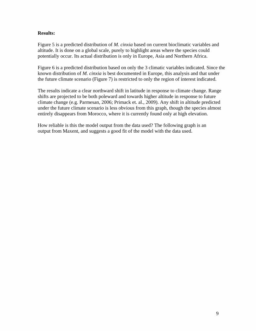
Results: Figure 5 is a predicted distribution of M. cinxia based on current bioclimatic variables and altitude. It is done on a global scale, purely to highlight areas where the species could potentially occur. Its actual distribution is only in Europe, Asia and Northern Africa. Figure 6 is a predicted distribution based on only the 3 climatic variables indicated. Since the known distribution of M. cinxia is best documented in Europe, this analysis and that under the future climate scenario (Figure 7) is restricted to only the region of interest indicated. The results indicate a clear northward shift in latitude in response to climate change. Range shifts are projected to be both poleward and towards higher altitude in response to future climate change (e.g. Parmesan, 2006; Primack et. al., 2009). Any shift in altitude predicted under the future climate scenario is less obvious from this graph, though the species almost entirely disappears from Morocco, where it is currently found only at high elevation. How reliable is this the model output from the data used? The following graph is an output from Maxent, and suggests a good fit of the model with the data used.

9

Figure 5: Maxent output of predicted current distribution of M. cinxia

Legend: The image uses colors to indicate predicted probability that conditions are suitable, with red indicating high probability of suitable conditions for the species, green indicating conditions typical of those where the species is found, and lighter shades of blue indicating low predicted probability of suitable conditions (Source: Maxent tutorial, http://www.cs.princeton.edu/~schapire/maxent/).

Figure 6: Maxent output of predicted current distribution of M. cinxia, using only 3 bioclimatic variables: annual mean temperature, maximum temperature of warmest month, and minimum temperature of coldest month (See figure 5 for legend).

Figure 7: Maxent output of predicted future distribution of M. cinxia, using only 3 bioclimatic variables: annual mean temperature, maximum temperature of warmest month, and minimum temperature of coldest month (See figure 5 for legend).

Figure 8: This graph shows the omission rate and predicted area as a function of the cumulative threshold. The omission rate is calculated on the training presence records. The omission rate should be close to the predicted omission, because of the definition of the cumulative threshold (see Maxent tutorial).

Conclusion: The methods used in this project, though very basic in their assumptions, may provide a useful tool for forecasting species response to climate change. As may be expected, M. cinxia is projected to move to higher latitudes and elevations under a changing climate. IPCC projections predict a warming of as much as 4°C across parts of the range of Melitaea cinxia (IPCC, 2007), over the course of this century. Species-specific models should help us to make more accurate predictions of climate change response within and among species. This project is intended as a small piece of the jigsaw of a fully integrated approach to studying the biological impacts of climate change, which must include detailed studies at the molecular, cellular and organismal levels (Portner et. al., 2006), as well as at the population, community and ecosystem levels.

13

References: Araújo, M.B. & Luoto, M. 2007. The importance of biotic interactions for modelling species distributions under climate change. GLOBAL ECOLOGY AND BIOGEOGRAPHY 16: 743-753. Crozier LG, 2004. Field transplants reveal summer constraints on a butterfly range expansion. OECOLOGIA 141 (1): 148-157. Hanski I, 1999. Metapopulation Ecology. Oxford University Press. Hawkins BA & Porter EE, 2003. Water-energy balance and the geographic pattern of species richness of western Palearctic butterflies. ECOLOGICAL ENTOMOLOGY 28 (6): 678-686. IPCC, 2007. Climate change 2007: The physical science basis. Intergovernmental panel on climate change (IPCC) WGI fourth assessment report. Lafranchis T, 2004. Butterflies of Europe. Diatheo. Lima FP et. al., 2007. Modelling past and present geographical distribution of the marine gastropod Patella rustica as a tool for exploring responses to environmental change. GLOBAL CHANGE BIOLOGY 13: 2065-2077. Parmesan C, 2006. Ecological and evolutionary responses to recent climate change. ANNUAL REVIEW OF ECOLOGY EVOLUTION AND SYSTEMATICS. 37: 637-669. Parmesan C et. al., 1999. Poleward shifts in geographical ranges of butterfly species associated with regional warming. NATURE 399: 579-583. Phillips SJ, Anderson RP & Schapire, RE, 2006. Maximum entropy modeling of species geographic distributions. ECOLOGICAL MODELLING190:231-259, 2006. Primack RB, et. al., 2009. Spatial and interspecific variability in phenological responses to warming temperatures. BIOLOGICAL CONSERVATION 142(11): 2569-2577. Pounds JA, et. al., 1999. Biological response to climate change on a tropical mountain. NATURE 398: 611-615. Thomas CD et. al., 2004. Extinction risk from climate change. NATURE 427: 145-148. Walther GR et. al., 2007. Palms tracking climate change. GLOBAL ECOLOGY AND BIOGEOGRAPHY. 16: 801-809.

14