approximation capabilities of interpretable fuzzy ... · hirofumi miyajima y1, noritaka shigeiy2,...

Approximation Capabilities of Interpretable FuzzyInference Systems

Hirofumi Miyajima†1 , Noritaka Shigei†2 , and Hiromi Miyajima†3

Abstract—Many studies on modeling of fuzzy inference sys-tems have been made. The issue of these studies is to constructautomatically fuzzy inference systems with interpretability andaccuracy from learning data based on metaheuristic methods.Since accuracy and interpretability are contradicting issues,there are some disadvantages for self-tuning method by meta-heuristic methods. Obvious drawbacks of the method arelack of interpretability and getting stuck in a shallow lo-cal minimum. Therefore, the conventional learning methodswith multi-objective fuzzy modeling and fuzzy modeling withconstrained parameters of the ranges have become popular.However, there are little studies on effective learning methodsof fuzzy inference systems dealing with interpretability andaccuracy. In this paper, we will propose a fuzzy inferencesystem with interpretability. Firstly, it is proved theoreticallythat the proposed method is a universal approximator ofcontinuous functions. Further, the capability of the proposedmodel learned by the steepest descend method is comparedwith the conventional models using function approximation andpattern classification problems in numerical simulation. Lastly,the proposed model is applied to obstacle avoidance and thecapability of interpretability is shown.

Index Terms—approximation capability, fuzzy inference, in-terpretability, universal approximator, obstacle avoidance.

I. INTRODUCTION

FUZZY inference systems are widely used in systemmodeling for the fields of classification, regression,

decision support system and control [1], [2]. Therefore,many studies on modeling of fuzzy inference systems havebeen made. The issue of these studies is to construct auto-matically fuzzy systems with interpretability and accuracyfrom learning data based on metaheuristic methods [3]–[7].Since accuracy and interpretability are contradicting issues,there are some disadvantages for self-tuning method bymetaheuristic methods. Obvious drawbacks of the methodare lack of interpretability and getting stuck in a shallowlocal minimum [8]. As metaheuristic methods, some novelmethods have been developed which 1) use GA and PSOto determine the structure of fuzzy systems [7], [9], 2) usefuzzy inference systems composed of small number of inputrule modules, such as SIRMs and DIRMs methods [10],[11], 3) use a self-organization or a vector quantizationtechnique to determine the initial assignment and 4) usecombined methods of them [4], [7], [9]. Since accuracy andinterpretability are conflicting goals, the conventional learn-ing methods with multi-objective fuzzy modeling and fuzzymodeling with constrained parameters of the ranges have

Affiliation: Graduate School of Science and Engineering, KagoshimaUniversity, 1-21-40 Korimoto, Kagoshima 890-0065, Japan

corresponding auther to provide email: [email protected]†1 email: [email protected]†2 email: [email protected]†3 email: [email protected]

become popular [7], [12]. However, there are little studieson effective learning methods of fuzzy inference systemssatisfying with interpretability and accuracy. It is desiredto develop effective fuzzy systems with interpretability torealize the linguistic processing of information which is theoriginal issue of fuzzy logic. Shi has proposed a fuzzyinference system with interpretability and accuracy [13].Further, Miyajima has proposed a generalized model of it[14]. However, there are no studies on the detailed capabilityof this type of model.

In this paper, we will propose a fuzzy inference sys-tem with interpretability and accuracy. Firstly, it is provedtheoretically that the proposed method is a universal ap-proximator of continuous functions. Further, the capabilityof the proposed model learned by the steepest descendmethod is compared with the conventional models usingfunction approximation and pattern classification problems innumerical simulation. Lastly, the proposed model is appliedto obstacle avoidance and the capability of interpretability isshown.

II. PRELIMINARIES

A. The conventional fuzzy inference model

The conventional fuzzy inference model is described [1].Let Zj = {1, · · · , j} for the positive integer j. Let R be theset of real numbers. Let x = (x1, · · · , xm) and yr be inputand output data, respectively, where xj∈R for j ∈ Zm andyr∈R. Then the rule of fuzzy inference model is expressedas

Ri : if x1 is Mi1 and · · · and xm is Mim

then y is fi(x1, · · ·, xm) (1)

, where i ∈ Zn is a rule number, j ∈ Zm is a variablenumber, Mij is a membership function of the antecedentpart, and fi(x1, · · ·, xm) is the function of the consequentpart.

A membership value of the antecedent part µj for inputx is expressed as

µi =

m∏j=1

Mij(xj). (2)

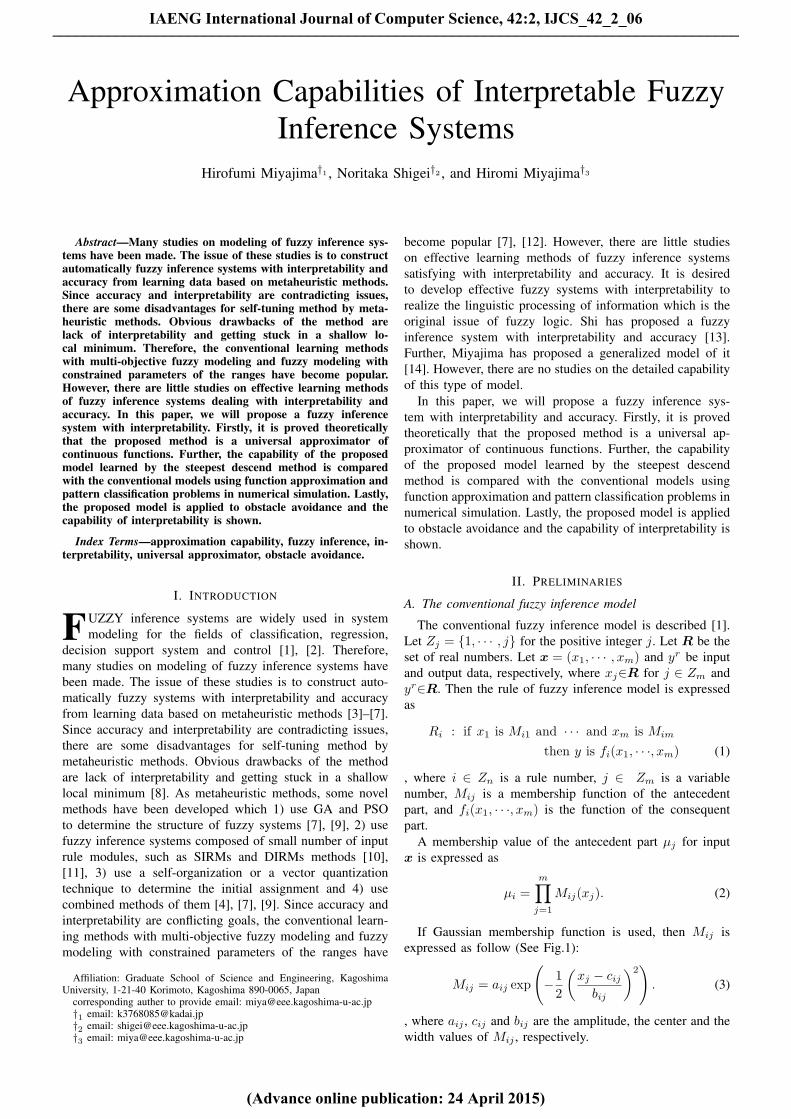
If Gaussian membership function is used, then Mij isexpressed as follow (See Fig.1):

Mij = aij exp

(−1

2

(xj − cij

bij

)2). (3)

, where aij , cij and bij are the amplitude, the center and thewidth values of Mij , respectively.

IAENG International Journal of Computer Science, 42:2, IJCS_42_2_06

(Advance online publication: 24 April 2015)

______________________________________________________________________________________

�

�

��

�

��

�

��

�

��

�

�

Fig. 1. The Gaussian membership function

The output y∗ of fuzzy inference is calculated by thefollowing equation:

y∗ =

∑ni=1 µi · fi∑n

i=1 µi. (4)

Specifically, simplified fuzzy inference model is known asone with fi(x1, · · ·, xm) = wi for i∈Zn, where wi∈R is areal number. The simplified fuzzy inference model is calledModel 1.

B. Learning algorithm for the conventional model

In order to construct the effective model, the conven-tional learning method is introduced. The objective functionE is defined to evaluate the inference error between thedesirable output yr and the inference output y∗. In thissection, we describe the conventional learning algorithm. LetD = {(xp

1, · · · , xpm, yrp)|p ∈ ZP } be the set of learning data.

The objective of learning is to minimize the following meansquare error(MSE):

E =1

P

P∑p=1

(y∗p − yrp)2. (5)

In order to minimize the objective function E, eachparameter α ∈ {aij , cij , bij , wi} is updated based on thedescent method as follows [1]:

α(t+ 1) = α(t)−Kα∂E

∂α(6)

where t is iteration time and Kα is a constant. WhenGaussian membership function with aij = 1 for i∈Zn andj∈Zm are used, the following relation holds [6].

∂E

∂wi=

µi∑ni=1 µi

· (y∗ − yr) (7)

∂E

∂cij=

µj∑ni=1 µi

· (y∗ − yr) · (wi − y∗) · xj − cijb2ij

(8)

∂E

∂bij=

µi∑ni=1 µi

· (y∗ − yr) · (wi − y∗) · (xj − cij)2

b3ij(9)

Then, the conventional learning algorithm is shown asbelow [1], [2], [6].

Learning Algorithm AStep A1 : The threshold θ of inference error and themaximum number of learning time Tmax are given. Theinitial assignment of fuzzy rules is set to equally intervals.Let n be the number of rules and n = dm for an integer d.Let t = 1.

Step A2 : The parameters bij , cij and wi are set to theinitial values.Step A3 : Let p = 1.Step A4 : A data (xp

1, · · ·, xpm, yrp)∈D is given.

Step A5 : From Eqs.(2) and (4), µi and y∗ are computed.Step A6 : Parameters cij , bij and wi are updated by Eqs.(8),(9) and (7).Step A7: If p = P then go to Step A8 and if p < P thengo to Step A4 with p←p+ 1.Step A8: Let E(t) be inference error at step t calculatedby Eq.(5). If E(t) > θ and t < Tmax then go to Step A3with t←t+1 else if E(t)≤θ and t≤Tmax then the algorithmterminates.Step A9: If t > Tmax and E(t) > θ then go to Step A2with n = dm as d←d+ 1 and t = 1.

C. The proposed model

It is known that Model 1 is effective, because all theparameters are adjusted by learning. On the other hand, allthe parameters move freely, so interpretability capability islow. Therefore, we propose the following model.

Ri1···im : if x1 is Mi11 and · · · and xm is Mimm

then y is fi1···im(x1, · · ·, xm) (10)

, where 1≤ij≤lj , Mijj(xj) is the membership function forxj and j∈Zm.

A membership value of the antecedent part µi1···im forinput x is expressed as

µi1···im =

m∏j=1

Mijj(xj) = Mi11(x1)·· · ··Mimm(xm) (11)

Then, the output y∗ is calculated by the following equa-tion.

y∗ =

∑i1· · ·∑

imµi1···imfi1···im(x1, · · ·, xm)∑

i1· · ·∑

imµi1···im

(12)

In this case, the model with fi1,···,im(x1· · ·, xm) =wi1,···,im and triangular membership function with aijj = 1has already proposed in the Ref. [13].

We will consider a model with fi1···im(x1, · · ·, xm) =wi1···im and Gaussian membership functions. The model iscalled Model 2.

[Example 1]Let us show an example of the proposed model with m =

2 and 1≤i1, i2≤2 as follows:

R11 : if x1 is M11 and x2 is M12 then y is w11




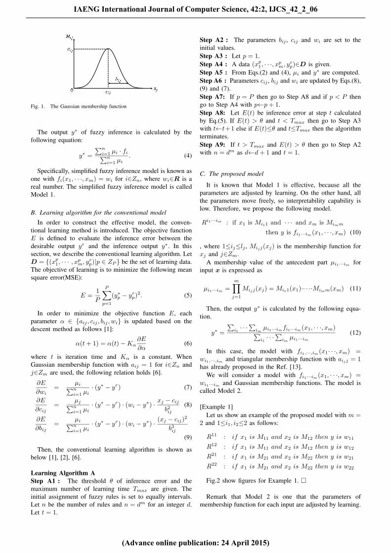
Fig.2 show figures for Example 1. □

Remark that Model 2 is one that the parameters ofmembership function for each input are adjusted by learning.



______________________________________________________________________________________

��

�

�

��

��

��

��

��

��

(a)Before learning.

�

�

��

��

��

��

��

��

(b)After learning.

Fig. 2. The figure to explain Model 2 with m = 2 and i1 = i2 = 2. Theassignment (a) of fuzzy rules for Model 2 is transformed into the assignment(b) after learning.

Learning equation for Model 2 is obtained as follows:

∂E

∂Mijj=∑i1

· · ·∑ij−1

∑ij+1

· · ·∑im

µi1···im∑i1· · ·∑

imµi1···im

· (y∗ − yr) · (y∗ − wi1···im)

(13)

∂E

∂wi1···im=

µi1···im∑i1· · ·∑

imµi1···im

· (y∗ − yr) (14)

When Gaussian membership function of Eq.(15) is used,the following equations for aijj , cijj and bijj are obtained;

Mijj(xj) = aijj exp

−1

2

m∑j=1

(xj − cijj)2

b2ijj

(15)

∂Mijj

∂aijj= exp

−1

2

m∑j=1

(xj − cijj)2

b2ijj

(16)

∂Mijj

∂cijj=

(xj − cijj)

b2ijjexp

−1

2

m∑j=1

(xj − cijj)2

b2ijj

(17)

∂Mijj

∂bijj=

(xj − cijj)2

b3ijjexp

−1

2

m∑j=1

(xj − cijj)2

b2ijj

(18)

Learning algorithm for the proposed model with aijj = 1is also defined using Eqs.(14), (17) and (18). Fig.2 explains

�

��

��

��

��

�

��

�

�

�

��

�

��

�

��

��

��

(a)Membership functions of the variable x1

�

��

��

��

��

�

��

�

�

�

��

�

��

�

��

(b)Membership functions of the variable x2

Fig. 3. The assignments of fuzzy rules of before and after learning forEq.(19).

the assignments of the antecedent parts of membershipfunctions for before and after learning.

Let us show an example for the practical movement ofmembership functions.[Example 2]

Let us consider the following function:

y =(2x1 + 4x2

2)(2x1 + 4x22 + 0.2)

37.2(19)

, where 0≤x1, x2≤1.In order to approximate Eq.(19), learning of the proposed

model with m = 2 and 1≤i1, i2≤3 is performed, where thenumber of learning data is 100.

Fig.3 shows the assignments of membership functionsafter learning, where waving and solid lines mean the assign-ments of membership functions before and after learning. □

Mamdani type model is special case of Model 2 [7].It is the model with the fixed parameters of antecedentpart of fuzzy rule and membership function assigned toequally intervals. The model is called Model 3. It has goodinterpretable capability, but the accuracy capability is law.Therefore, TSK model with the weight of linear functionfi(x1, · · ·, xm) is introduced as a generalized model ofModel 3 [13]. The model is called Model 4.

III. FUZZY INFERENCE SYSTEM AS UNIVERSALAPPROXIMATOR

In this section, the universal approximation capabilitiesof Model 1, 2, 3 and 4 are discussed using the well-known Stone-Weierstrass Theorem. See Ref. [2] about themathematical terms.[Stone-Weierstrass Theorem] [2]Let S be a compact set with m dimensions, and C(S) be



______________________________________________________________________________________

a set of all continuous real-valued functions on S. Let Φbe the set of continuous real-valued functions satisfying theconditions:(i) Identity function : The constant function f(x) = 1 is inΦ.(ii) Separability : For any two points x1,x2∈S and x1 ̸=x2,there exists a f∈Φ such that f(x1)̸=f(x2).(iii) Algebraic closure : For any f, g∈Φ and α, β∈R, thefunctions f ·g and αf + βg are in Φ.

Then, Φ is dense in C(S). In other words, for any ε > 0and any function g∈C(S), there is a function f∈Φ such that

|g(x)− f(x)| < ε

for all x∈S.

It means that the set Φ satisfying the above conditions canapproximate any continuous function with any accuracy.Since the sets of RBF and Model 1 are satisfied withthe conditions of Stone-Weierstrass Theorem, they hold foruniversal approximation capabilities [2], [16], [17]. Further,we can show the result about Model 2 in the following.[Theorem]

Let Φ be the set of all functions that can be computed byModel 2 on a compact set S⊂Rm as follows:Let

Φl1···lm = { f(x) =

∑i1· · ·∑

im

∏j Mijj(xj)wi1···im∑

i1· · ·∑

imMijj(xj)

, wi1···wm , aijj , cijj , bijj∈R,x∈S}

for Mijj(xj) = aijj exp

(−1

2

(xj−cijj

bijj

)2)and

Φ =∞∪

l1=1

· · ·∞∪

lm=1

Φl1···lm (20)

Then Φ is dense in C(S).[Proof]

In order to prove the result, it is shown that three condi-tions of Stone-Weierstrass Theorem are satisfied.(i)The function f(x) = 1 for x∈S is in Φ, because it can beconsidered as a Gaussian function with infinite variable b.(ii)The set Φ satisfies with the separability since the expo-nential function is monotonic.(iii)Let f and g be two functions in Φ and be represented as

f(x) =

∑i1· · ·∑

im

∏j M

fijj

(xj)wfi1···im∑

i1· · ·∑

im

∏j M

fijj

(xj)(21)

g(x) =

∑l1· · ·∑

lm

∏j M

gljj

(xj)wgl1···lm∑

l1· · ·∑

lm

∏j M

gljj

(xj)(22)

for

Mfijj

(xj) = afijj exp

−1

2

(xj − cfijj

bfijj

)2 (23)

Mgljj

(xj) = agljj exp

−1

2

(xj − cgljj

bgljj

)2 (24)

Then, we show αf + βg∈Φ and f ·g∈Φ for α, β∈R.

We define

Mfgij ljj

(xj) = Mfijj

(xj)·Mglj(xj)

= afgij ljj exp

−1

2

(xj − cfgij ljj

bfgij ljj

)2(25)

wfg1i1···iml1···lm = wf

i1···im + wgl1···lm (26)

wfg2i1···iml1···lm = wf

i1···im ·wgl1·lm (27)

, where afgij ljj , cfgij ljj

, bfgij ljj , wfg1i1···wim l1···lm , wfg2

i1···iml1···lm∈R.By using these values,

αf + βg

=

∑i1· · ·∑

im

∑l1· · ·∑

lm

∏j M

fgij ljj

(xj)wfg1i1···iml1···lm∑

i1· · ·∑

im

∑l1· · ·∑

lm

∏j M

fgij ljj

(xj)

(28)

f ·g

=

∑i1· · ·∑

im

∑l1· · ·∑

lm

∏j M

fgij ljj

(xj)wfg2i1···iml1···lm∑

i1· · ·∑

im

∑l1· · ·∑

lm

∏j M

fgij ljj

(xj)

(29)

Further, Eqs.(28) and (29) have the same form as Model 2.Therefore, (αf + βg) and f ·g∈Φ hold.□

[Remarks]Remark that the results using Stone-Weierstrass Theoremhold only for Model 1 and 2 with fi(x1· · ·xm) = wi andGaussian membership function. On the other hand, Stone-Weierstrass Theorem does not always hold for Model 3, 4and the models with triangular membership function, becausethe multiplicative condition fails. Further, it is an existencetheorem and there is another problem whether we can getthe system with high accuracy. Therefore, we need effectivelearning algorithm. Learning Algorithm A is a learningalgorithm based on the steepest descend method.

IV. NUMERICAL SIMULATIONS

In this section, three kinds of simulations are performedto compare the capability of the proposed model with theconventional model for learning method based on steepestdescend method. In the simulations, let aij = 1 and aijj = 1for i∈Zn and j∈Zm.

A. Function approximation

This simulation uses four systems specified by the follow-ing functions with [0, 1]×[0, 1].

y = sin(πx31)·x2 (30)

y =sin(2πx3

1)· cos(πx2) + 1

2(31)

y =1.9(1.35 + ex1 sin(13(x1 − 0.6)2)·e−x2 sin(7x2))

7(32)

y =sin(10(x1 − 0.5)2 + 10(x2 − 0.5)2) + 1.0

2(33)

The condition of the simulation is shown in Table I. Thevalue θ is 1.0×10−5 and the numbers of learning and test



______________________________________________________________________________________

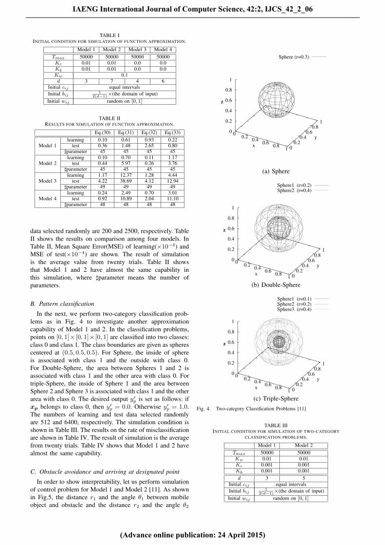
TABLE IINITIAL CONDITION FOR SIMULATION OF FUNCTION APPROXIMATION.

Model 1 Model 2 Model 3 Model 4Tmax 50000 50000 50000 50000Kc 0.01 0.01 0.0 0.0Kb 0.01 0.01 0.0 0.0Kw 0.1d 3 7 4 6

Initial cij equal intervalsInitial bij 1

2(d−1)×(the domain of input)

Initial wij random on [0, 1]

TABLE IIRESULTS FOR SIMULATION OF FUNCTION APPROXIMATION.

Eq.(30) Eq.(31) Eq.(32) Eq.(33)learning 0.10 0.61 0.93 0.22

Model 1 test 0.36 1.48 2.65 0.80♯parameter 45 45 45 45

learning 0.10 0.70 0.11 1.17Model 2 test 0.44 5.97 0.26 3.76

♯parameter 45 45 45 45learning 1.17 12.37 1.28 4.44

Model 3 test 4.22 38.69 4.12 12.94♯parameter 49 49 49 49

learning 0.24 2.49 0.70 3.01Model 4 test 0.92 10.89 2.04 11.10

♯parameter 48 48 48 48

data selected randomly are 200 and 2500, respectively. TableII shows the results on comparison among four models. InTable II, Mean Square Error(MSE) of learning(×10−4) andMSE of test(×10−4) are shown. The result of simulationis the average value from twenty trials. Table II showsthat Model 1 and 2 have almost the same capability inthis simulation, where ♯parameter means the number ofparameters.

B. Pattern classification

In the next, we perform two-category classification prob-lems as in Fig. 4 to investigate another approximationcapability of Model 1 and 2. In the classification problems,points on [0, 1]× [0, 1]× [0, 1] are classified into two classes:class 0 and class 1. The class boundaries are given as spherescentered at (0.5, 0.5, 0.5). For Sphere, the inside of sphereis associated with class 1 and the outside with class 0.For Double-Sphere, the area between Spheres 1 and 2 isassociated with class 1 and the other area with class 0. Fortriple-Sphere, the inside of Sphere 1 and the area betweenSphere 2 and Sphere 3 is associated with class 1 and the otherarea with class 0. The desired output yrp is set as follows: ifxp belongs to class 0, then yrp = 0.0. Otherwise yrp = 1.0.The numbers of learning and test data selected randomlyare 512 and 6400, respectively. The simulation condition isshown in Table III. The results on the rate of misclassificationare shown in Table IV. The result of simulation is the averagefrom twenty trials. Table IV shows that Model 1 and 2 havealmost the same capability.

C. Obstacle avoidance and arriving at designated point

In order to show interpretability, let us perform simulationof control problem for Model 1 and Model 2 [11]. As shownin Fig.5, the distance r1 and the angle θ1 between mobileobject and obstacle and the distance r2 and the angle θ2

0 0.2

0.4 0.6

0.8 1 0

0.2 0.4

0.6 0.8

1

0

0.2

0.4

0.6

0.8

1

z

Sphere (r=0.3)

x

y

z

(a) Sphere

00.2

0.40.6

0.81 0

0.20.4

0.60.8

1

0

0.2

0.4

0.6

0.8

1

z

Sphere1 (r=0.2)Sphere2 (r=0.4)

x

y

z

(b) Double-Sphere

00.2

0.40.6

0.81 0

0.20.4

0.60.8

1

0

0.2

0.4

0.6

0.8

1

z

Sphere1 (r=0.1)Sphere2 (r=0.2)Sphere3 (r=0.4)

x

y

z

(c) Triple-SphereFig. 4. Two-category Classification Problems [11]

TABLE IIIINITIAL CONDITION FOR SIMULATION OF TWO-CATEGORY

CLASSIFICATION PROBLEMS.

Model 1 Model 2Tmax 50000 50000Kw 0.01 0.01Kc 0.001 0.001Kb 0.001 0.001d 3 5



Initial wij random on [0, 1]



______________________________________________________________________________________

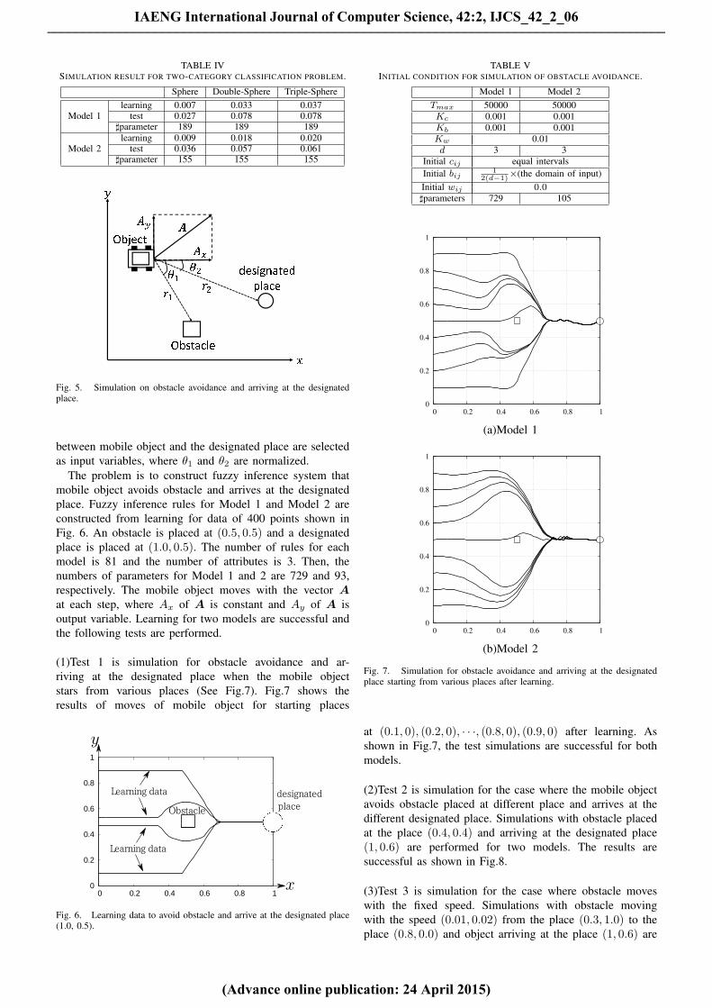
TABLE IVSIMULATION RESULT FOR TWO-CATEGORY CLASSIFICATION PROBLEM.

Sphere Double-Sphere Triple-Spherelearning 0.007 0.033 0.037

Model 1 test 0.027 0.078 0.078♯parameter 189 189 189

learning 0.009 0.018 0.020Model 2 test 0.036 0.057 0.061

♯parameter 155 155 155

�

�

�

�

�

�

�

�

�

�

�

�

�

��

��

��

��

�

�

Fig. 5. Simulation on obstacle avoidance and arriving at the designatedplace.

between mobile object and the designated place are selectedas input variables, where θ1 and θ2 are normalized.

The problem is to construct fuzzy inference system thatmobile object avoids obstacle and arrives at the designatedplace. Fuzzy inference rules for Model 1 and Model 2 areconstructed from learning for data of 400 points shown inFig. 6. An obstacle is placed at (0.5, 0.5) and a designatedplace is placed at (1.0, 0.5). The number of rules for eachmodel is 81 and the number of attributes is 3. Then, thenumbers of parameters for Model 1 and 2 are 729 and 93,respectively. The mobile object moves with the vector Aat each step, where Ax of A is constant and Ay of A isoutput variable. Learning for two models are successful andthe following tests are performed.

(1)Test 1 is simulation for obstacle avoidance and ar-riving at the designated place when the mobile objectstars from various places (See Fig.7). Fig.7 shows theresults of moves of mobile object for starting places

Fig. 6. Learning data to avoid obstacle and arrive at the designated place(1.0, 0.5).

TABLE VINITIAL CONDITION FOR SIMULATION OF OBSTACLE AVOIDANCE.

Model 1 Model 2Tmax 50000 50000Kc 0.001 0.001Kb 0.001 0.001Kw 0.01d 3 3



Initial wij 0.0♯parameters 729 105

0

0.2

0.4

0.6

0.8

1

0 0.2 0.4 0.6 0.8 1

(a)Model 1

0

0.2

0.4

0.6

0.8

1

0 0.2 0.4 0.6 0.8 1

(b)Model 2

Fig. 7. Simulation for obstacle avoidance and arriving at the designatedplace starting from various places after learning.

at (0.1, 0), (0.2, 0), · · ·, (0.8, 0), (0.9, 0) after learning. Asshown in Fig.7, the test simulations are successful for bothmodels.

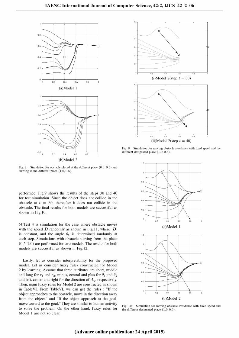
(2)Test 2 is simulation for the case where the mobile objectavoids obstacle placed at different place and arrives at thedifferent designated place. Simulations with obstacle placedat the place (0.4, 0.4) and arriving at the designated place(1, 0.6) are performed for two models. The results aresuccessful as shown in Fig.8.

(3)Test 3 is simulation for the case where obstacle moveswith the fixed speed. Simulations with obstacle movingwith the speed (0.01, 0.02) from the place (0.3, 1.0) to theplace (0.8, 0.0) and object arriving at the place (1, 0.6) are



______________________________________________________________________________________

0

0.2

0.4

0.6

0.8

1

0 0.2 0.4 0.6 0.8 1

(a)Model 1

-0.2

0

0.2

0.4

0.6

0.8

1

0 0.2 0.4 0.6 0.8 1

(b)Model 2

Fig. 8. Simulation for obstacle placed at the different place (0.4, 0.4) andarriving at the different place (1.0, 0.6).

performed. Fig.9 shows the results of the steps 30 and 40for test simulation. Since the object does not collide in theobstacle at t = 30, thereafter it does not collide in theobstacle. The final results for both models are successful asshown in Fig.10.

(4)Test 4 is simulation for the case where obstacle moveswith the speed B randomly as shown in Fig.11, where |B|is constant, and the angle θb is determined randomly ateach step. Simulations with obstacle starting from the place(0.5, 1.0) are performed for two models. The results for bothmodels are successful as shown in Fig.12.

Lastly, let us consider interpretability for the proposedmodel. Let us consider fuzzy rules constructed for Model2 by learning. Assume that three attributes are short, middleand long for r1 and r2, minus, central and plus for θ1 and θ2and left, center and right for the direction of Ay , respectively.Then, main fuzzy rules for Model 2 are constructed as shownin TableVI. From TableVI, we can get the rules : ”If theobject approaches to the obstacle, move in the direction awayfrom the object.” and ”If the object approach to the goal,move toward to the goal.” They are similar to human activityto solve the problem. On the other hand, fuzzy rules forModel 1 are not so clear.

0

0.2

0.4

0.6

0.8

1

1.2

0 0.2 0.4 0.6 0.8 1

(i)Model 2(step t = 30)

0

0.2

0.4

0.6

0.8

1

1.2

0 0.2 0.4 0.6 0.8 1

(ii)Model 2(step t = 40)

Fig. 9. Simulation for moving obstacle avoidance with fixed speed and thedifferent designated place (1.0, 0.6).

0

0.2

0.4

0.6

0.8

1

1.2

0 0.2 0.4 0.6 0.8 1

(a)Model 1

0

0.2

0.4

0.6

0.8

1

1.2

0 0.2 0.4 0.6 0.8 1

(b)Model 2

Fig. 10. Simulation for moving obstacle avoidance with fixed speed andthe different designated place (1.0, 0.6).



______________________________________________________________________________________

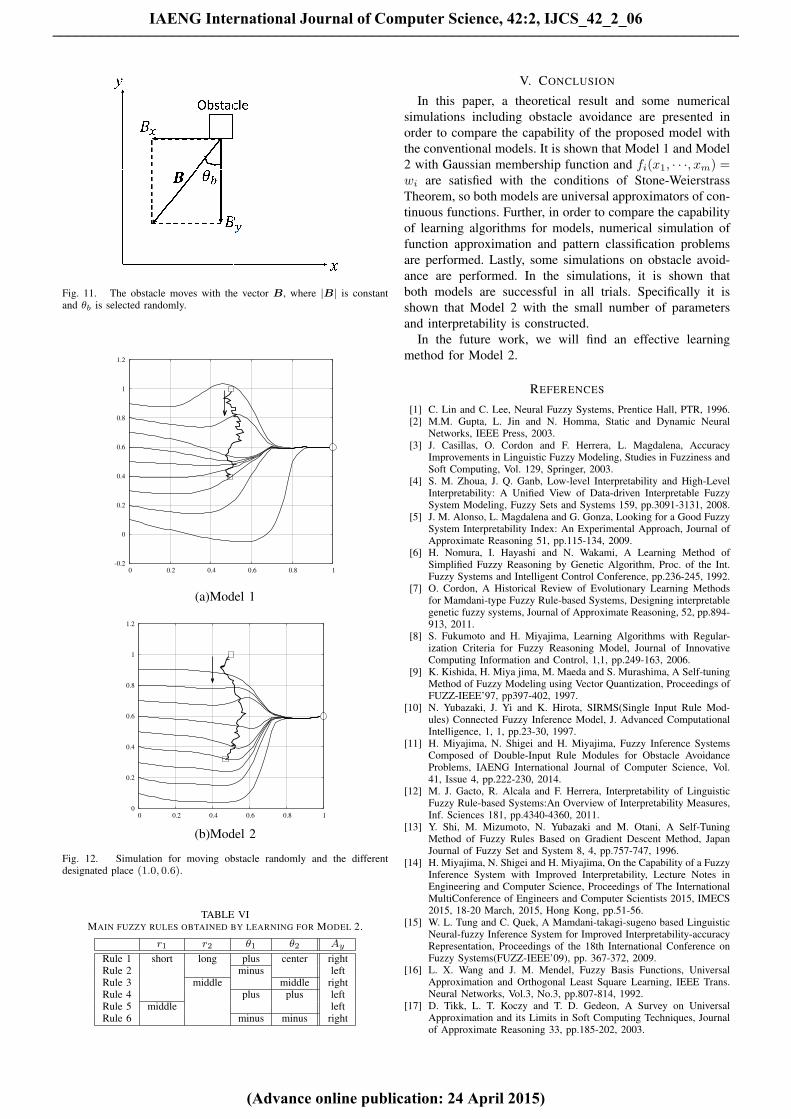
Fig. 11. The obstacle moves with the vector B, where |B| is constantand θb is selected randomly.

-0.2

0

0.2

0.4

0.6

0.8

1

1.2

0 0.2 0.4 0.6 0.8 1

(a)Model 1

0

0.2

0.4

0.6

0.8

1

1.2

0 0.2 0.4 0.6 0.8 1

(b)Model 2

Fig. 12. Simulation for moving obstacle randomly and the differentdesignated place (1.0, 0.6).

TABLE VIMAIN FUZZY RULES OBTAINED BY LEARNING FOR MODEL 2.

r1 r2 θ1 θ2 Ay

Rule 1 short long plus center rightRule 2 minus leftRule 3 middle middle rightRule 4 plus plus leftRule 5 middle leftRule 6 minus minus right

V. CONCLUSION

In this paper, a theoretical result and some numericalsimulations including obstacle avoidance are presented inorder to compare the capability of the proposed model withthe conventional models. It is shown that Model 1 and Model2 with Gaussian membership function and fi(x1, · · ·, xm) =wi are satisfied with the conditions of Stone-WeierstrassTheorem, so both models are universal approximators of con-tinuous functions. Further, in order to compare the capabilityof learning algorithms for models, numerical simulation offunction approximation and pattern classification problemsare performed. Lastly, some simulations on obstacle avoid-ance are performed. In the simulations, it is shown thatboth models are successful in all trials. Specifically it isshown that Model 2 with the small number of parametersand interpretability is constructed.

In the future work, we will find an effective learningmethod for Model 2.

REFERENCES

[1] C. Lin and C. Lee, Neural Fuzzy Systems, Prentice Hall, PTR, 1996.[2] M.M. Gupta, L. Jin and N. Homma, Static and Dynamic Neural

Networks, IEEE Press, 2003.[3] J. Casillas, O. Cordon and F. Herrera, L. Magdalena, Accuracy

Improvements in Linguistic Fuzzy Modeling, Studies in Fuzziness andSoft Computing, Vol. 129, Springer, 2003.

[4] S. M. Zhoua, J. Q. Ganb, Low-level Interpretability and High-LevelInterpretability: A Unified View of Data-driven Interpretable FuzzySystem Modeling, Fuzzy Sets and Systems 159, pp.3091-3131, 2008.

[5] J. M. Alonso, L. Magdalena and G. Gonza, Looking for a Good FuzzySystem Interpretability Index: An Experimental Approach, Journal ofApproximate Reasoning 51, pp.115-134, 2009.

[6] H. Nomura, I. Hayashi and N. Wakami, A Learning Method ofSimplified Fuzzy Reasoning by Genetic Algorithm, Proc. of the Int.Fuzzy Systems and Intelligent Control Conference, pp.236-245, 1992.

[7] O. Cordon, A Historical Review of Evolutionary Learning Methodsfor Mamdani-type Fuzzy Rule-based Systems, Designing interpretablegenetic fuzzy systems, Journal of Approximate Reasoning, 52, pp.894-913, 2011.

[8] S. Fukumoto and H. Miyajima, Learning Algorithms with Regular-ization Criteria for Fuzzy Reasoning Model, Journal of InnovativeComputing Information and Control, 1,1, pp.249-163, 2006.

[9] K. Kishida, H. Miya jima, M. Maeda and S. Murashima, A Self-tuningMethod of Fuzzy Modeling using Vector Quantization, Proceedings ofFUZZ-IEEE’97, pp397-402, 1997.

[10] N. Yubazaki, J. Yi and K. Hirota, SIRMS(Single Input Rule Mod-ules) Connected Fuzzy Inference Model, J. Advanced ComputationalIntelligence, 1, 1, pp.23-30, 1997.

[11] H. Miyajima, N. Shigei and H. Miyajima, Fuzzy Inference SystemsComposed of Double-Input Rule Modules for Obstacle AvoidanceProblems, IAENG International Journal of Computer Science, Vol.41, Issue 4, pp.222-230, 2014.

[12] M. J. Gacto, R. Alcala and F. Herrera, Interpretability of LinguisticFuzzy Rule-based Systems:An Overview of Interpretability Measures,Inf. Sciences 181, pp.4340-4360, 2011.

[13] Y. Shi, M. Mizumoto, N. Yubazaki and M. Otani, A Self-TuningMethod of Fuzzy Rules Based on Gradient Descent Method, JapanJournal of Fuzzy Set and System 8, 4, pp.757-747, 1996.

[14] H. Miyajima, N. Shigei and H. Miyajima, On the Capability of a FuzzyInference System with Improved Interpretability, Lecture Notes inEngineering and Computer Science, Proceedings of The InternationalMultiConference of Engineers and Computer Scientists 2015, IMECS2015, 18-20 March, 2015, Hong Kong, pp.51-56.

[15] W. L. Tung and C. Quek, A Mamdani-takagi-sugeno based LinguisticNeural-fuzzy Inference System for Improved Interpretability-accuracyRepresentation, Proceedings of the 18th International Conference onFuzzy Systems(FUZZ-IEEE’09), pp. 367-372, 2009.

[16] L. X. Wang and J. M. Mendel, Fuzzy Basis Functions, UniversalApproximation and Orthogonal Least Square Learning, IEEE Trans.Neural Networks, Vol.3, No.3, pp.807-814, 1992.

[17] D. Tikk, L. T. Koczy and T. D. Gedeon, A Survey on UniversalApproximation and its Limits in Soft Computing Techniques, Journalof Approximate Reasoning 33, pp.185-202, 2003.



______________________________________________________________________________________

approximation capabilities of interpretable fuzzy ... · hirofumi miyajima y1, noritaka shigeiy2,...

Documents