april 2010 rff dp 10-16 discussion paper · april 2010 rff dp 10-16 energy-efficiency ... excluded...

1616 P St. NW Washington, DC 20036 202-328-5000 www.rff.org

Apri l 2010 RFF DP 10-16

Energy-Efficiency Program Evaluations

Opportunities for Learning and Inputs to Incentive Mechanisms

Noah Ka ufman and Karen Pa lmer

DIS

CU

SSIO

N P

APE

R

© 2010 Resources for the Future. All rights reserved. No portion of this paper may be reproduced without permission of the authors.

Discussion papers are research materials circulated by their authors for purposes of information and discussion. They have not necessarily undergone formal peer review.

Energy-Efficiency Program Evaluations: Opportunities for Learning and Inputs to Incentive Mechanisms

Noah Kaufman and Karen Palmer

Abstract We analyze the evaluations of California energy-efficiency programs to assess the effectiveness

of these evaluations in: 1) improving our understanding of their performance and 2) providing a check on utility incentives to overstate energy savings. We find that third-party evaluations are useful tools to achieve both ends because the programs largely did not meet their energy-savings projections, and the utility-reported savings estimates are systematically higher than the evaluated savings estimates. We also find evidence that the choice of the third-party evaluator was influential in determining the estimate of evaluated savings.

Key Words: energy efficiency, third-party evaluation, energy-savings measurement

JEL Classification Numbers: L94, L95, L51

Contents

Introduction ............................................................................................................................. 1

The California Performance Incentive Mechanism ............................................................. 4

Data Sources ............................................................................................................................ 6

Summary of the Data .............................................................................................................. 8

Comparison of the Differences in Energy-Savings Estimates ........................................... 12

Causes of the Differences in Energy-Savings Estimates .................................................... 17

Discussion, Limitations, and Conclusions ........................................................................... 31

References .............................................................................................................................. 32

Appendix ................................................................................................................................ 35

Resources for the Future Kaufman and Palmer

1

Energy-Efficiency Program Evaluations: Opportunities for Learning and Inputs to Incentive Mechanisms

Noah Kaufman and Karen Palmer∗

Introduction

Energy efficiency is a key component of local and national strategies to reduce energy use and combat global warming. The National Action Plan for Energy Efficiency (2008)—a consortium of electric and gas utilities, utility regulators, and other U.S. stakeholders—identifies the goal of achieving all cost-effective energy-efficiency measures in the country by 2025, representing more than $500 billion in net savings. Realizing these substantial efficiencies in such a short time period will require a massive effort to successfully identify opportunities and implement energy-efficiency programs. Many states and countries already have begun this effort.

This paper will focus on ex-post measurements of the savings that can be attributed to energy-efficiency programs. The third-party program evaluations that supply these measurements are a controversial component of the effort to improve energy efficiency in this country. The objective of this paper is to provide an assessment of the information from these energy-efficiency program evaluations using empirical data from California.

The importance of energy-efficiency program evaluations is derived largely from the unfortunate reality that energy savings are extremely difficult to measure. It is common for projections and estimates of energy savings to be calculated by program implementers using simple formulas, such as the number of units of an efficiency measure installed multiplied by the presumed energy savings per unit. Because these formulas fail to take into account consumer behavior and other factors, they are highly imprecise. Better measurement of energy savings requires the monitoring of actual energy usage and an answer to the counterfactual question: how much energy would have been used in the absence of an energy-efficiency program? Ex-post program evaluations go beyond the simple formulas described above, using measurements of actual consumer behavior to calculate energy savings. The more sophisticated measurements

∗ Kaufman ([email protected]) is a former RFF summer intern and a graduate student in the economics department at the University of Texas at Austin. Palmer ([email protected]) is the Darius Gaskins Senior Fellow at Resources for the Future. We are grateful to Joe Loper, Michael Rufo, Shanjun Li, Juha Siikamaki and seminar participants at the University of Texas at Austin for their helpful comments on earlier versions of this paper.


2

provided by the evaluations are useful for two primary reasons. First, evaluations provide an opportunity to learn more about the relative performance of the different types of energy-efficiency measures and programs as well as the policies that facilitate the implementation and effectiveness of these efforts. While energy-efficiency programs and efforts to estimate the savings they produce have existed for several decades, our understanding of the most cost-effective methods to achieve energy savings is still in its infancy. A great deal of trial and error and policy experimentation must take place to improve this understanding, so it is important to learn when these experiments have failed and succeeded. Designers and implementers of energy-efficiency programs will rely on these conclusions in revising and expanding programs. Moreover, the savings measurements in ex-post evaluations are themselves an inexact science. The more evaluations that are conducted, the better we can determine how precise and useful these measurements are compared to ex ante projections.

A second motivation for conducting energy-efficiency program evaluations stems from the independence of the third-party evaluators. This independence enables their evaluations to function as a component of a regulatory structure known as a “performance incentive mechanism,” which we now explain briefly.

The performance of energy-efficiency programs depends on the actions of the local electric and gas utilities that oversee the programs. A challenge for utility regulators is how to provide incentives for utilities to promote efforts to save energy. Under cost-of-service regulation, electric and gas utilities do not have an incentive to maximize their customers’ energy savings. In fact, utilities’ profit margins typically decrease as customer energy use decreases, so a fundamental conflict of interest lies between the utilities’ desire to sell energy and the public interest in conserving energy. Removing this conflict of interest is the motivation behind methods of decoupling utilities’ revenues from their sales. Under a decoupling mechanism, rates are adjusted so that utilities do not lose money as electricity sales decline and cannot earn extra revenue if actual sales are above projected sales.

While decoupling mechanisms remove the incentive for utilities to resist energy-conservation efforts, some states have now gone a step further in providing rewards for utilities that successfully promote these efforts. A performance-incentive mechanism is a regulatory framework that provides utilities with the opportunity to earn a profit from energy-efficiency activities in their service territories, often by allocating to them a small percentage of the value of the energy savings. In the case of California, the performance-incentive mechanism that is


3

currently in place includes threshold values for savings above which the incentive payment to the utility increases dramatically.

Performance-incentive mechanisms also provide an incentive for utilities to claim as much energy savings as possible, in order to earn greater profits. These greater profits are directly at the expense of the ratepayers in the utilities’ service territories. The difficulty of verifying or refuting energy-savings claims puts electricity consumers and regulators at a disadvantage in assessing savings reported by utilities. For this reason, independent ex-post measurements can be a valuable check on the utilities’ incentive to overestimate energy savings.

In this paper, we analyze the results of the recently completed evaluations of the 2004–2005 California utility energy-efficiency programs compared to both ex-ante savings projections and the results reported by the electric and gas utilities. It is extremely rare to find in the public domain a dataset with comparable projected, reported, and evaluated savings data. This unique dataset enables us to analyze both objectives of energy-efficiency program evaluations described above: First, related to the use of evaluations as an opportunity for learning, we compare the ex-ante savings projections with the ex-post evaluated savings measurements. Second, related to the use of evaluations as a check on the incentives of the electric and gas utilities, we compare the utility-reported savings estimates with the ex-post evaluated savings measurements. Using techniques of statistics and econometrics, we identify what differentiates energy-efficiency programs that have had higher evaluated savings compared to predicted savings than others, and what differentiates programs that have had independent evaluations confirm or exceed the utility-reported energy savings.

We aim to give policymakers and regulators a better idea of the benefits of incorporating independent evaluations into their performance-incentive mechanisms, and to provide valuable information to those who will be designing and implementing energy-efficiency programs in the near future.

We find that the energy-efficiency programs in the 2004–2005 California program cycle did not meet ex-ante expectations in terms of electricity savings, gas savings, or peak-demand savings. We also find that the utility-reported electricity savings estimates are systematically higher than the third-party evaluated savings estimates, indicating that the incentive to overstate savings may affect the utilities’ reports. Interestingly, the particular contractor chosen to conduct the evaluation (or an unobservable correlated with this choice) appears to be an important determinant of the level of the evaluated savings estimates when compared to both the ex-ante projections and the utility-reported results. Specifically, the largest and most commonly used


4

evaluators are associated with the programs with relatively lower evaluated savings estimates, suggesting that these particular evaluators may provide a greater scrutiny of savings than that provided by other evaluators.

The California Performance Incentive Mechanism

Since the 1970s, California has been at the forefront of U.S. pursuits of energy-efficiency goals. Supply shortages, air pollution, and increasing concerns regarding the emissions of greenhouse gases into the atmosphere have heightened the emphasis on energy efficiency in California in recent years. As a result, the state has focused a great deal of resources on efforts to conserve energy.

California’s energy-efficiency programs are administered largely by the states’ four investor-owned utilities (IOUs) with the oversight of the California Public Utilities Commission (CPUC). The state’s performance-incentive mechanism, known as the Risk-Reward Incentive Mechanism (RRIM), awards profits to an IOU based on the savings produced by the energy-efficiency programs in its service area compared to predetermined annual savings goals. The energy savings are monetized and divided among the IOU shareholders, in the form of profits to the utility, and the California ratepayers in the form of lower energy bills over time. Specifically, if the utility achieved more than 85 percent of its savings goals, the incentive payment increased from 0 percent to 9 percent of the value of energy savings. If the savings exceeded 100 percent of savings goals, the incentive payment increased from 9 percent to 12 percent (CPUC 2007). Though the RRIM was not formally adopted until 2006, the measures of energy savings were to be cumulative, starting in 2004, to ensure that the IOUs would focus on long-term goals. Therefore, the RRIM would encompass the performance of the 2004–2005 programs.1

Evaluation, measurement, and verification (EM&V) of energy savings has been a major component of California’s energy-efficiency efforts. The CPUC has stated, “[R]atepayers will only be required to share net benefits with (IOU) shareholders to the extent that those net benefits actually materialize, based on EM&V results” (CPUC 2007, pages 12-13). For the 2004-

1 Indeed, the performance of the 2004–2005 programs was included in determining intermim payments to the California IOUs under the RRIM in verification reports released in February and October 2009 (CPUC 2009a, 2009c). However, a November 2009 proposed ruling of the CPUC states that the 2004–2005 programs should be excluded from determining future payments to the IOU because the savings are not directly reconcilable with 2006–2008 programs (CPUC 2009d).


5

–2005 program cycle, CPUC released a list of all contractors approved to perform EM&V work, stating, “Contractors whose relationships to programs might compromise or appear to compromise an independent evaluation are not included on the list” (CPUC 2004, page 1). Both the particular choice of contractor and the EM&V plan were then subject to the approval of the CPUC.

This RRIM recently has generated much controversy. The California IOUs have received a portion of the profits due to them under the RRIM based on their own reports of energy savings, while the remaining portion has been withheld until independent evaluations confirm these savings estimates. The initial energy-savings verification report under the RRIM (which included the nearly completed evaluations from the 2004–2005 program cycle) was first released in August 2008 and concluded that three of the four IOUs had failed to meet the energy savings thresholds that would have been required to earn any payouts under the RRIM (CPUC 2009a). The IOUs have complained about the delays of the EM&V process and the fairness of the evaluations’ use of ex-post savings measurements to determine the performance of the energy-efficiency programs. They have argued that ex-post evaluations should be used only to update the energy-savings goals for each program cycle and improve future program designs. Profits, the IOUs claim, should be regular and predictable, and contingent only on periodic verifications of program costs and installations. In contrast, ratepayer advocates have argued that IOUs should only earn profits if and when it is shown by an independent evaluator that energy savings attributable to an energy-efficiency program have occurred. Otherwise, ratepayers will likely pay for savings that have not actually been achieved.

The CPUC has stood in the middle of this controversy, attempting to balance two counteracting goals. On one hand, it is important to provide sufficient and attainable rewards to the IOUs so that they will be motivated to produce actual energy savings. On the other hand, the CPUC has the responsibility to minimize the costs to the California ratepayers and taxpayers of providing these rewards. These costs include both the IOUs’ profits (which otherwise would have been returned to ratepayers in the form of lower rates) and the administrative costs of the programs and related bureaucracy. The ex-post evaluations unquestionably have decreased the predictability of a portion of IOU earnings and added delays and costs to the process. The evaluations from the 2004–2005 cycle of energy-efficiency programs were only finalized in 2008, and millions of dollars were spent on performing these evaluations. However, a clear conflict of interest exists in making IOU profits contingent on the utilities own reports of energy


6

savings rather than savings that have been verified by ex-post evaluations conducted by third parties.

Going forward, CPUC regulators must determine whether the benefits of the third-party evaluations are worth the costs. Thus far, empirical evidence has not been available to compare IOU-reported and third-party evaluated results and thus assess the specific impact that the evaluations have had on the process. The 2004–2005 program cycle in California is an exception.

Data Sources

The information in this report is primarily from two sources: 1) 118 third-party ex-post evaluations of energy-efficiency programs in California from the 2004–2005 program cycle, obtained from the appendices of the Energy Efficiency 2006–2007 Verification Report (CPUC 2009a); 2) the filings of the four IOUs (Pacific Gas & Electric, Southern California Edison, SoCalGas, San Diego Gas & Electric) relating to these same 118 energy-efficiency programs, obtained from the CPUC’s Energy Efficiency Groupware website (http://eega.cpuc.ca.gov).

Law required that third-party contractors evaluate the 2004–2005 California energy-efficiency programs per the CPUC’s (2003b) Energy Efficiency Policy Manual to measure the level of energy and peak demand savings achieved; measure cost-effectiveness; provide up-front market assessments and baseline analysis; provide ongoing feedback and corrective, constructive guidance regarding the implementation of programs; and help to assess whether need for the program was ongoing.

The IOUs chose the contractors that conducted the evaluations. However, the CPUC provided the IOUs with a list of contractors from which they could make their selections, and the commission also had the right to approve or deny each selection based on the independence and qualifications of the contractor for the specific evaluation efforts it would undertake. According to the CPUC, the key criteria for the choice of the evaluation teams were the professional experience and expertise of the contractors. Smaller programs required just one contractor to complete an evaluation, while larger and more complex programs required the collaboration of a number of contractors.

While more than 200 programs were funded through the public-goods charge (TecMarket Works Framework Team 2007), some were for informational or educational purposes and did not have energy-savings goals or require impact evaluations. In contrast, the evaluated programs included in these data are mainly “resource acquisition” programs, which provide incentives to


7

customers to upgrade to more energy-efficient equipment. The full list of evaluated programs can be found in the Appendix. These programs include a variety of different measures, such as efforts to install high-efficiency faucets in food service establishments, no-cost energy audits for residential homes, and the distribution of free energy-efficient compact fluorescent bulbs and fluorescent torchiere lamps.

In its Energy Efficiency 2006–2007 Verification Report, which included the results of the nearly complete evaluations from the 2004–2005 energy efficiency program cycle, the CPUC (2009a) provided information on the impact evaluations of 118 energy-efficiency programs from 2004–2005, including links to evaluations of 112 of the programs on the CPUC website. A single evaluation often contained the energy impacts of more than one energy-efficiency program, which occurred when the same (or virtually the same) program was implemented in different IOU service territories. Nearly all the evaluations contained standard “Impact Reporting Tables,” providing “gross projected” and “net evaluated” annual energy and gas savings for each program.2

Beside the annual savings information from these tables, we compiled the following information on each program where available: IOU involved in the implementation of the program, third-party contractor(s) that conducted the evaluation, evaluation methodology, customer class, electricity or gas end use, net-to-gross (NTG) ratio(s) used by the program, whether an independent NTG analysis was undertaken, and projected and realized total program costs3 and benefits.

The independent contractors used a wide array of methodologies to measure energy savings in the evaluations. The CPUC (2003b) Energy Efficiency Policy Manual required adherence to the International Performance Measurement & Verification Protocol (IPMVP) for the M&V portion of the evaluation. The IPMVP provides four evaluation methodologies from which the evaluator could choose to perform an “energy impact analysis,” ranging from “partial

2 In this context, “gross” savings are calculated as the difference in energy use by program participants before and after their participation in the program. “Net” savings controls for savings that would have occurred for these participants over the same time period whether the program was offered or not (TecMarket Works Framework Team 2004). Note that this definition of “net” savings does not adjust for spillover effects, which are energy savings that occur due to investments made by non-participants who became aware of opportunities to save energy as a result of the program. 3 Costs are as defined by the “total resource cost” test and are different from those defined by the “program administer cost” test in that they include those costs incurred by participating customers.


8

field measurement” to “fully calibrated simulations” of energy use (IPMVP 2002). Certain evaluations were clearly more rigorous in their measurements than others. Nevertheless, they all provided an additional level of rigor when compared to the savings estimates of the IOUs.

The California IOUs were also required to track the performance of their own 2004–2005 energy-efficiency programs. These reports are publicly available on the CPUC Energy Efficiency Groupware website and are our second main source of data. From these reports, we compiled the following information that the IOUs reported: original program budget, EM&V budget, total program expenditures, EM&V expenditures, annual net energy goals, annual net energy impacts, NTG ratio(s), and projected and realized total program costs and benefits.

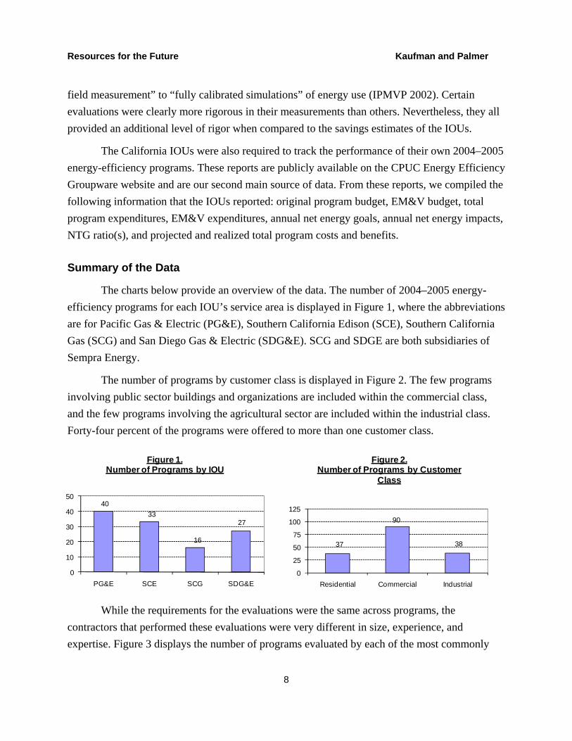
Summary of the Data

The charts below provide an overview of the data. The number of 2004–2005 energy-efficiency programs for each IOU’s service area is displayed in Figure 1, where the abbreviations are for Pacific Gas & Electric (PG&E), Southern California Edison (SCE), Southern California Gas (SCG) and San Diego Gas & Electric (SDG&E). SCG and SDGE are both subsidiaries of Sempra Energy.

The number of programs by customer class is displayed in Figure 2. The few programs involving public sector buildings and organizations are included within the commercial class, and the few programs involving the agricultural sector are included within the industrial class. Forty-four percent of the programs were offered to more than one customer class.

While the requirements for the evaluations were the same across programs, the contractors that performed these evaluations were very different in size, experience, and expertise. Figure 3 displays the number of programs evaluated by each of the most commonly

4033

16

27

0

10

20

30

40

50

PG&E SCE SCG SDG&E

Figure 1.Number of Programs by IOU

37

90

38

0

25

50

75

100

125

Residential Commercial Industrial

Figure 2. Number of Programs by Customer

Class


9

used third-party evaluators. Two large firms were the most popularly used evaluators by a wide margin. (We refer to them as “Large Firm A” and Large Firm B” throughout this paper instead of using their real names.) These publicly traded corporations have thousands of employees in more than 20 countries around the world and hundreds of millions of dollars in annual revenue. On the other end of the spectrum are two private companies, one with seven staff members and another with a staff of two in a single office in California. Not surprisingly given the relative size of the companies, the large firms tended to evaluate the larger programs. The average budget of a program evaluated by either Large Firm A or Large Firm B was $9.1 million, whereas the average budget of the remaining programs was $3.6 million. More than one evaluator assessed thirty-seven percent of the programs (but we made no attempt to discern which evaluators performed which functions for these programs).

Program budgets and expenditures, as reported by the IOUs, are displayed in Figure 4. Programs had spent an average of 75 percent of their total budgets by the time the final IOU reports on the programs were issued.

26 25

11 10 9 8

0

10

20

30

40

50

Large Firm A Large Firm B Firm C Firm D Firm E Firm F

Figure 3.Number of Programs by Evaluator


10

The IPMVP provides evaluators with four options on how to measure energy impacts. Option A, “Partially Measured Retrofit Isolation,” requires that savings be determined by short-term or continuous field measurements of energy use. For Option A, some parameters can be taken from second-hand sources (“stipulated parameters”), as long as the potential error from doing so is not significant. Option B, “Retrofit Isolation,” is the same as Option A, except no parameters may be stipulated. Option C is called “Whole Facility,” and savings are determined by directly measuring energy use at the whole facility level rather than using a particular energy source on which a program focuses. Option C is useful for programs that affect many different systems within a building. Finally, Option D, “Calibrated Simulation,” requires that savings be determined via simulation of the energy use of components or the whole facility (IPMVP 2002). Figure 5 displays the number of energy-efficiency programs that claimed to use each option described above. Some larger programs claimed to use more than one option. Twenty-two evaluations did not state which option was chosen, and a few evaluations stated that they did not use any options of the IPMVP, generally due to budgetary concerns. It should be noted that we did not attempt to determine how rigorously the evaluations followed the guidelines for each option set forth in the IPMVP. Moreover, these options comprised just one component of the evaluations and were not necessarily reflective of the rigor of the full evaluations.

The IOU filings break out the total program budgets and expenditures by category, one of which is EM&V spending. Figure 6 displays the mean and median percentages of the total ex-ante budget and total ex-post expenditures allocated to EM&V spending, as reported by the IOUs.

4,620

2,336

3,428

1,930

01,0002,0003,0004,0005,0006,000

Mean Median

Figure 4.Program Budgets and Expenditures ($000s)

Budget Expenditures


11

Notes: IPMVP=International Performance Measurement and Verification Protocol; EM&V=evaluation,

measurement, and verification.

Programs were at different stages in their development at the beginning of the 2004–2005 energy-efficiency program cycle. While some programs already had been functioning for years, others did not begin accruing savings until the middle of the 2004–2005 cycle. Since the evaluations supplied energy savings information by year, we could determine approximately when the savings began to accrue. Figure 7 displays this information.

Figure 8 displays the difference between IOU-reported and evaluated cost-effectiveness measures. The total resources cost (TRC) ratio is defined as the benefits divided by the costs of a demand-side management energy-efficiency program. The benefits used to calculate the TRC ratio are the avoided supply costs and the reduction in transmission, distribution, generation, and capacity costs valued at marginal cost. The costs used to calculate the TRC ratio are the program

31

55

21

5

0

20

40

60

80

Jan 2004 Mid 2004 Jan 2005 Post Jan 2005

Figure 7.Time Period when Savings began to Accrue

3128

8 6

0

10

20

30

40

Option A Option B Option C Option D

Figure 5.IPMVP Methodology

4.3% 4.0%3.9% 3.8%

0.0%

1.0%

2.0%

3.0%

4.0%

5.0%

6.0%

Mean Median

Figure 6.EM&V Spending / Total Spending

Budgeted IOU-Reported Expenditure


12

costs paid by both the IOU and the program participants plus the increase in supply costs for the periods in which load is increased. Figure 8 only includes data for 45 percent of the programs because many evaluations did not track cost-effectiveness. (Even though we have IOU-reported data for virtually all programs, these data are omitted from this chart so that the evaluated and reported values are directly comparable.)

Comparison of the Differences in Energy-Savings Estimates

The objective of this section is to compare the three compiled estimates of energy savings (projected, IOU reported, and evaluated) to assess the benefits of the program evaluations. The comparison of the ex-ante and ex-post savings estimates provides an indication of how useful the evaluations are as an opportunity to learn about the success or failure of the programs. The comparison of the IOU-reported and evaluated savings estimates provides an indication of how useful the evaluations are as a check on the incentives of the IOUs.

We provide a summary of the savings estimates in Table 1. It reports measures of savings4 with three different metrics: megawatt hours (MWh), megawatts (MW), and therms. The MWh and therm measurements are the aggregate amounts of electricity and gas, respectively, used over a period of time. The MW measurement is the demand for electricity at

4 The IOU filings report a single value for cumulative annual net energy savings, which is calculated by the formula: (total units installed)*(energy savings per unit)*(NTG ratio). The evaulations provide annual net energy savings for each year, starting in 2004. We have used 2006 energy savings throughout this paper because they include all installations from 2004 and 2005, and therefore are most directly comparable to the reported “annual” values. All energy savings are net of free riders.

1.471.28

2.10 2.21

0.00

0.50

1.00

1.50

2.00

2.50

Mean Median

Figure 8.Total Resource Cost (TRC) Test(Program Benefits / Program Costs)

Evaluated Reported


13

peak usage hours, which is of crucial importance because electricity is not storable, so avoiding power outages requires sufficient generating capacity to serve the demand of customers at peak times. Since peak electricity demand is inherently more difficult to measure than aggregate energy use, it is likely that the estimates of savings in MW are relatively less precise.

We define a “realization rate” as ex-post estimated savings (from either the IOU reports or the third-party evaluations) divided by ex-ante projected savings. The “IOU accuracy ratio” is defined as evaluated savings divided by IOU-reported savings. The confidence intervals on the median value (right-most column) are obtained using the binomial method.

From Table 1, we draw two primary conclusions relating to the two potential benefits of evaluations described above. First, the evaluated realization rates show that evaluated savings were substantially lower than projected savings—none of the median confidence intervals for the evaluated realization rates include 100 percent. These evaluations provide valuable revisions of the ex-ante projections of savings and therefore may offer very different conclusions as to the performance of specific types of program.

Second, large differences exist between the IOU-reported and evaluated savings estimates. In particular, evaluated savings are systematically lower than IOU-reported savings.

Table 1.Summary Statistics

Median 95%Weighted # obs # obs Confidence

Total 1 Mean Median median 2 >100% <100% IntervalRealization rate MWh IOU-reported 87.1% 91.8% 97.7% 91.2% 48 55 (80%-107%) Evaluated 67.0% 75.8% 68.9% 62.9% 21 76 (63%-82%)Realization rate MW IOU-reported 82.6% 92.0% 97.5% 92.9% 45 54 (81%-103%) Evaluated 69.3% 83.7% 87.2% 65.2% 25 67 (79%-92%)Realization rate therms IOU-reported 117.5% 117.4% 100.6% 110.8% 32 29 (81%-110%) Evaluated 58.3% 108.8% 75.8% 57.2% 12 52 (60%-85%)

IOU accuracy ratio MWh 85.3% 160.9% 87.1% 60.1% 38 60 (81%-99%) MW 91.3% 142.4% 92.6% 71.0% 38 56 (85%-105%) Therms 47.0% 1189.0% 73.9% 47.6% 16 43 (56%-85%)

IOU = investor owned utility; MWh = megawatt hours; MW = megawatts.Realization rates are defined as ex-post estimated savings divided by ex-ante projected savings.IOU accuracy ratio is defined as evaluated savings divided by IOU-reported savings.Savings comparisons are between "2006" data from evaluations and "annual" data from IOU reports.

1 For a consistent comparison, a program's savings data is only included in the sum if both the numerator and the denoninator are observed. 2 Each observation is weighted by percentage of total savings. The ratios (Realization Rates or IOU Accurancy Ratios) are then ordered from smallest

to largest, and the cumulative sum of the weights is calculated for each observation. The weighted median is the average of the first observations above and below the cumulative sum of weights equal to 50%.


14

Specifically, total evaluated MWh savings were 85 percent of total reported MWh savings, total evaluated MW savings were 91 percent of total reported MW savings, and total evaluated therm savings were 47 percent of total reported therm savings. For the 95 percent median confidence intervals on the evaluated-to-reported savings ratio, only savings measured in MW have an interval that includes 100 percent. Therefore, the evaluations appear to be valuable in their role as a check on the IOUs’ incentive to overestimate energy savings: if these evaluations were not undertaken and the 2004–2005 savings were included in the RRIM, the IOUs’ would have been eligible for payouts under the California RRIM that the evaluations suggest they had not truly earned.

Finally, we offer three other notes regarding the data in Table 1. The “median” and “mean” values substantially differ, showing that outliers influence these data. We discuss this issue in more detail below. Also, total realizations rates are generally lower than both mean and median realization rates. This reflects lower realization rates for the largest programs (because small and large programs are implicitly given equal weighting in the calculation of the median and mean realization rates). Lastly, the IOU accuracy ratio is much higher for MW savings than it is for either measure of energy savings. This higher level of accuracy in reported estimates of peak period savings is likely due to the limited time duration of peak demand periods and thus the limited potential for behavioral factors to cause savings to deviate from more engineering based estimates.

Non-Parametric Tests

The benefits of the energy-efficiency program evaluations both as an opportunity for learning about how to improve program performance and as a component of a performance-incentive mechanism is contingent on whether the evaluated savings estimates significantly differ from other estimates of savings. In this section, we perform statistical tests to analyze these differences.

Because of the relatively small number of observations for each savings metric, we provide non-parametric tests of the hypotheses that the IOU-reported savings estimates are equal to the evaluated savings estimates, and that the ex-ante projected savings estimates are equal to the evaluated savings estimates. The advantage of using these tests, as compared to a standard t-test, is that they require minimal assumptions regarding the underlying distribution of data.

The Wilcoxon Matched-Pairs Signed Ranks test is used to determine whether differences exist between groups of paired data points. The null hypothesis is that the differences between


15

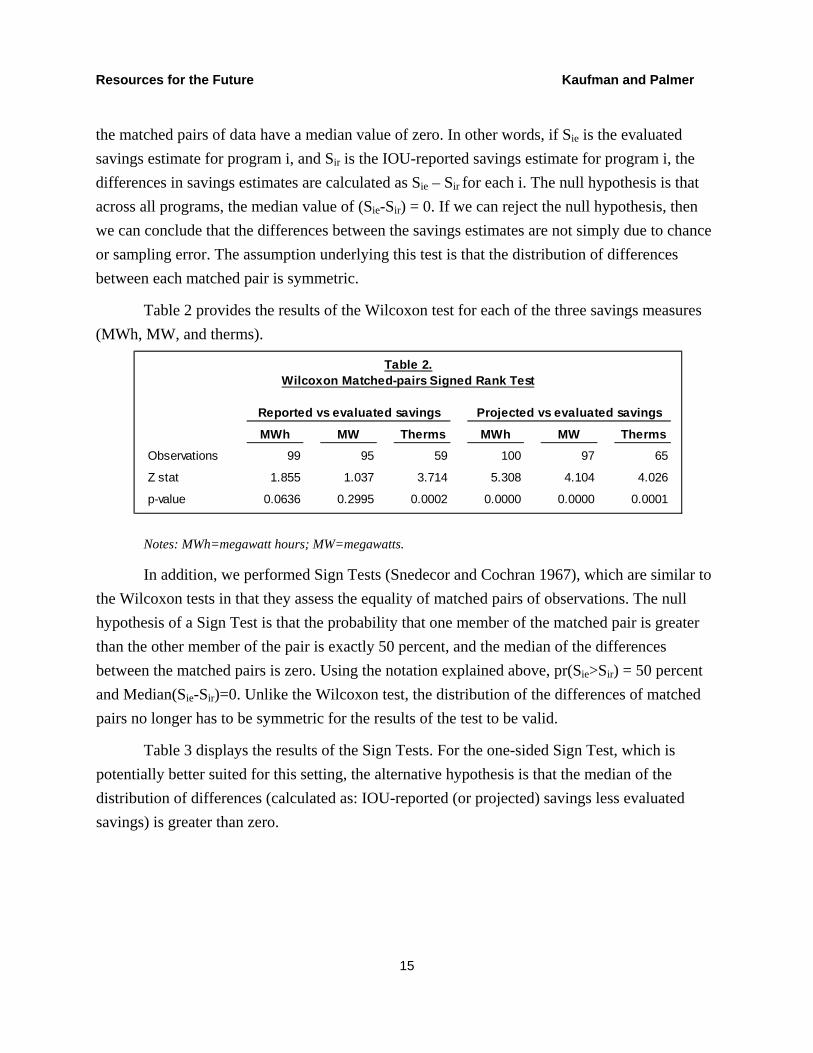
the matched pairs of data have a median value of zero. In other words, if Sie is the evaluated savings estimate for program i, and Sir is the IOU-reported savings estimate for program i, the differences in savings estimates are calculated as Sie – Sir for each i. The null hypothesis is that across all programs, the median value of (Sie-Sir) = 0. If we can reject the null hypothesis, then we can conclude that the differences between the savings estimates are not simply due to chance or sampling error. The assumption underlying this test is that the distribution of differences between each matched pair is symmetric.

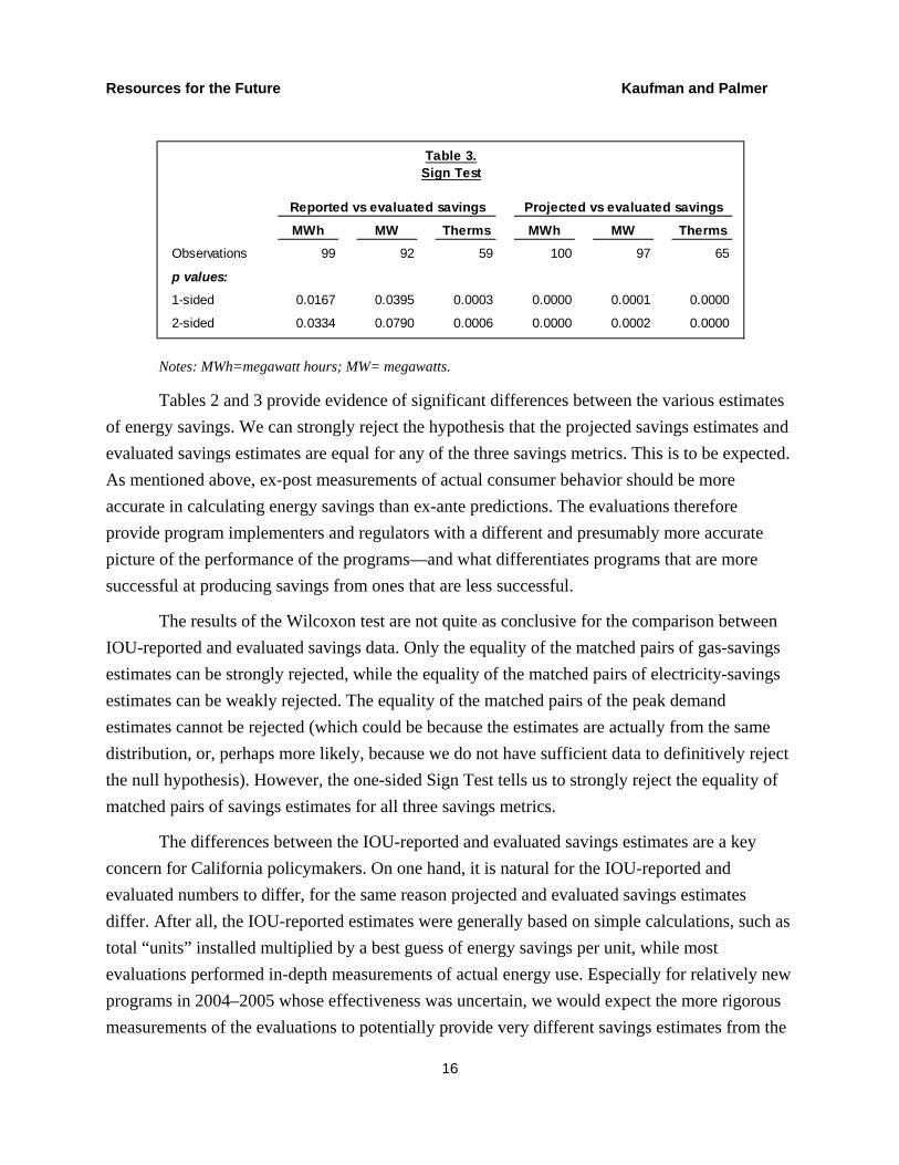
Table 2 provides the results of the Wilcoxon test for each of the three savings measures (MWh, MW, and therms).

Notes: MWh=megawatt hours; MW=megawatts.

In addition, we performed Sign Tests (Snedecor and Cochran 1967), which are similar to the Wilcoxon tests in that they assess the equality of matched pairs of observations. The null hypothesis of a Sign Test is that the probability that one member of the matched pair is greater than the other member of the pair is exactly 50 percent, and the median of the differences between the matched pairs is zero. Using the notation explained above, pr(Sie>Sir) = 50 percent and Median(Sie-Sir)=0. Unlike the Wilcoxon test, the distribution of the differences of matched pairs no longer has to be symmetric for the results of the test to be valid.

Table 3 displays the results of the Sign Tests. For the one-sided Sign Test, which is potentially better suited for this setting, the alternative hypothesis is that the median of the distribution of differences (calculated as: IOU-reported (or projected) savings less evaluated savings) is greater than zero.

Table 2.Wilcoxon Matched-pairs Signed Rank Test

Reported vs evaluated savings Projected vs evaluated savings

MWh MW Therms MWh MW Therms

Observations 99 95 59 100 97 65

Z stat 1.855 1.037 3.714 5.308 4.104 4.026

p-value 0.0636 0.2995 0.0002 0.0000 0.0000 0.0001


16

Notes: MWh=megawatt hours; MW= megawatts.

Tables 2 and 3 provide evidence of significant differences between the various estimates of energy savings. We can strongly reject the hypothesis that the projected savings estimates and evaluated savings estimates are equal for any of the three savings metrics. This is to be expected. As mentioned above, ex-post measurements of actual consumer behavior should be more accurate in calculating energy savings than ex-ante predictions. The evaluations therefore provide program implementers and regulators with a different and presumably more accurate picture of the performance of the programs—and what differentiates programs that are more successful at producing savings from ones that are less successful.

The results of the Wilcoxon test are not quite as conclusive for the comparison between IOU-reported and evaluated savings data. Only the equality of the matched pairs of gas-savings estimates can be strongly rejected, while the equality of the matched pairs of electricity-savings estimates can be weakly rejected. The equality of the matched pairs of the peak demand estimates cannot be rejected (which could be because the estimates are actually from the same distribution, or, perhaps more likely, because we do not have sufficient data to definitively reject the null hypothesis). However, the one-sided Sign Test tells us to strongly reject the equality of matched pairs of savings estimates for all three savings metrics.

The differences between the IOU-reported and evaluated savings estimates are a key concern for California policymakers. On one hand, it is natural for the IOU-reported and evaluated numbers to differ, for the same reason projected and evaluated savings estimates differ. After all, the IOU-reported estimates were generally based on simple calculations, such as total “units” installed multiplied by a best guess of energy savings per unit, while most evaluations performed in-depth measurements of actual energy use. Especially for relatively new programs in 2004–2005 whose effectiveness was uncertain, we would expect the more rigorous measurements of the evaluations to potentially provide very different savings estimates from the

Table 3.Sign Test

Reported vs evaluated savings Projected vs evaluated savings

MWh MW Therms MWh MW Therms

Observations 99 92 59 100 97 65

p values:

1-sided 0.0167 0.0395 0.0003 0.0000 0.0001 0.0000

2-sided 0.0334 0.0790 0.0006 0.0000 0.0002 0.0000


17

IOU reports. If the IOU reports underestimated savings as often as they overestimated savings, the evaluations would not provide a check on the incentives of IOUs in a performance incentive mechanism.

However, the results above show a clear trend for the reported values to be higher than the evaluated values, which could reflect the incentives of the IOUs to overestimate savings in order to increase profits. Putting a check on this incentive is the primary motive for CPUC to continue to include these evaluations as a component of the performance incentive mechanism. Inflated savings values would be costly to California ratepayers. The IOUs would have been eligible for millions of dollars in profits under the RRIM if ex-post savings estimates were based on the IOU-reports alone.

The IOUs have argued that the evaluations should not be a component of a performance-incentive mechanism as they have been in the past. During the 2004–2005 program cycle, the IOUs were well aware that their savings estimates would be subject to revision by the evaluations. These data are therefore not necessarily representative of how the IOUs would have behaved if the evaluations had not been a part of the incentive mechanism. It seems likely that the incentive of the IOUs to overestimate savings would be greater in the future if they knew the evaluations would not be used as a check on their savings estimates under the RRIM.

Finally, it is important to note that in assessing the benefits of independent evaluations, these data represent only half the story. Performing ex-post evaluations of energy-efficiency programs has costs as well as benefits. This section has pointed out the benefits of these evaluations both in terms of opportunities for learning and as a check on the incentive of the IOUs to overestimate savings. For a regulator such as the CPUC to determine how to best use these evaluations, it needs to compare these benefits to the costs of the evaluation process to the taxpayers and ratepayers.

Causes of the Differences in Energy-Savings Estimates

Using the dataset described above, we proceed to the second objective of this paper, which is to attempt to answer the following two questions: 1) what differentiates an energy-efficiency program that is successful in meeting its ex-ante goals from one that is not?; and 2)


18

what differentiates an energy-efficiency program that has its IOU-reported savings estimates confirmed by an independent evaluation from one that does not?5

Question 1 Analysis

To answer Question 1, we analyze the realization rates (defined as evaluated savings divided by projected savings) across programs. Higher realization rates imply more successful programs compared to expectations. Recall that realization rates of close to 100 percent imply that the evaluations provide little new information for future program designers and implementers (in addition to what was provided by the projections). Table 4 provides median and mean values for realization rates for the three savings metrics across programs with the different characteristics described above. These values can be compared to the mean and median values for all programs, highlighted and bolded in the top row of Table 4. Due to the limited number of observations, we urge caution in interpreting the results reported in Table 4. Nevertheless, some findings are interesting. For instance, the programs in SDG&E’s service territory generally are less successful than those in PG&E’s or SCE’s. The electricity savings from SCG’s programs are based on a very small number of observations because SCG does not sell electricity, and so it only reported electricity savings for a handful of programs. Programs that were in existence from the start of the 2004–2005 cycle were relatively more successful in meeting their annual savings projections than those that commenced operations later in the cycle. As would be expected, programs that spent a smaller percentage of their budget were less successful in meeting their MW and MWh savings goals (but curiously, this relationship does not hold for therm savings). More cost-effective programs in general had higher realization rates. Programs evaluated by Large Firm A or Large Firm B, as well as programs evaluated by multiple evaluators, tended to be less successful in meeting their ex-ante projections. Also, evaluations that measured energy savings using Option B of the IPMVP were relatively less successful in meeting their ex-ante projections than were evaluations that used Option A. This result is expected because the two options are identical besides the additional rigor that is

5 Note that we do not imply that the evaluations have necessarily measured the true value of program savings but only that that the evaluated savings estimates should be more accurate than the reported savings estimates because of the increased rigor in the savings calculations and the independence of the third-party evaluators.


19

required by Option B, which does not permit stipulated parameters. This suggests that the more rigorous are the evaluations, the more valuable they are as replacements for ex-ante projections.6

Notes: PG&E=Pacific Gas & Electric; SCE=Southern California Edison; SCG=Southern California Gas; SDG&E=San Diego Gas & Electric; TRC=total resources cost ratio; EM&V=evaluation, measurement, and verification; IPMVP=International Performance Measurement & Verification Protocol.

6 The independent contractors that performed the evaluations generally were selected and required to provide a plan for the evalution (subject to CPUC approval) near the beginning of the 2004–2005 program cycle. Therefore, we have no reason to believe that the choice of evaluation methodology was endogeneous. Endogeneity would be a concern if programs that were underperforming were more likely to be evaluated with more rigorous methods.

Table 4.What differentiates a program that is successful in meeting its goals from one that is not?

(All values below represent evaluated realization rates: evaluated / projected savings)

MWh savings MW savings Therm savingsObs Median Mean Obs Median Mean Obs Median Mean

ALL PROGRAMS 97 68.9% 75.8% 92 87.2% 83.7% 65 75.8% 108.8%

Utility: PG&E 36 81.3% 82.9% 35 87.9% 89.4% 26 81.4% 88.3% SCE 28 68.3% 72.7% 26 90.1% 80.4% 10 81.0% 286.1% SCG 8 66.9% 69.2% 7 100.4% 80.9% 15 71.8% 63.8% SDG&E 25 62.7% 71.0% 24 78.3% 79.9% 14 60.4% 68.5%

Customer class: Residential 34 75.5% 77.8% 34 83.4% 82.3% 23 78.5% 77.7% Commercial 78 68.9% 74.4% 73 86.3% 84.4% 54 78.5% 117.7% Industrial 31 63.2% 70.1% 27 89.1% 87.0% 24 85.4% 164.1%

Savings began in: Beginning of 2004 27 82.3% 80.9% 25 96.5% 91.9% 19 83.3% 190.5% Middle of 2004 46 65.1% 69.8% 45 83.1% 77.5% 29 68.2% 63.4% Beginning of 2005 19 72.9% 80.3% 18 84.6% 83.2% 14 92.7% 106.5% Post-Beginning 2005 5 69.5% 85.8% 4 85.2% 104.7% 3 26.7% 42.2%

Budget vs expenditures: > 90% Budget Spent 51 81.3% 82.2% 50 93.4% 89.5% 30 73.8% 74.5% < 90% Budget Spent 46 57.5% 68.7% 42 80.7% 76.9% 35 76.5% 138.3%

Cost-effectiveness: Reported TRC>1 84 68.9% 77.3% 80 89.9% 88.3% 49 71.8% 117.8% Reported TRC<1 13 69.5% 65.6% 12 57.2% 53.4% 16 84.5% 81.3%

Evaluated TRC>1 82 77.7% 80.6% 78 90.3% 89.9% 48 78.5% 127.0% Evaluated TRC<1 15 52.6% 49.5% 14 35.5% 49.3% 17 41.2% 57.5%

Evaluator: Large Firm A 21 62.7% 65.9% 19 89.5% 84.6% 11 67.5% 75.1% Large Firm B 25 53.2% 51.7% 24 60.1% 59.3% 16 57.2% 51.4% All others 65 82.3% 84.2% 62 93.3% 90.0% 45 78.5% 129.2%

Single evaluator 61 82.3% 85.4% 60 89.2% 89.2% 44 76.1% 119.6% Multiple evaluators 36 59.1% 59.5% 32 69.9% 73.4% 21 69.6% 86.3%

Spending on EM&V: EM&V budget > 4% of total budget 46 75.4% 76.8% 43 86.6% 83.9% 23 88.6% 99.8% EM&V budget < 4% of total budget 47 67.1% 73.0% 45 83.7% 81.5% 40 69.1% 118.9%

EM&V expenditure > 4% of total expenditure 57 68.8% 77.2% 54 86.4% 79.5% 39 78.5% 138.7% EM&V expenditure < 4% of total expenditure 40 70.1% 73.7% 38 89.9% 89.7% 26 71.8% 64.0%

IPMVP methodology: Option A - Partially measured retrofit isolation 32 83.0% 82.8% 29 97.9% 93.6% 24 77.2% 88.3% Option B - Retrofit isolation 24 60.8% 65.0% 22 89.9% 84.2% 15 67.5% 63.2% Option C - Whole facility 9 67.5% 69.3% 9 70.8% 81.4% 7 83.5% 73.9% Option D - Calibrated simulation 5 67.5% 79.3% 5 101.0% 114.7% 2 60.4% 60.4%


20

Regression Analysis—Question 1:

We ran regression analyses to gain further insight into what differentiates an energy-efficiency program that is successful compared to its expectations from one that falls short. The dependent variable in these regressions is the evaluated realization rate (defined as the ratio of evaluated savings to projected savings). As independent variables, we tested many characteristics of the programs and evaluation process for which summary data are provided above. The advantage of the regression approach is that it allows us to isolate the effects of particular characteristics holding everything else constant.

We used a number of different regression models to account for the limitations of these data. Among these limitations are small sample sizes, outliers in the dependent variable observations, and the potential non-independence of the error terms of certain observations. Due to insufficient data, we did not run regressions on the gas savings metric.

The full model is of the form:

&

&

where “PG&E,” “SCE,” and SCG” are dummy variables representing the relevant IOU (with SDG&E omitted); “Commercial,” “Industrial,” and the three interaction terms are dummy variables representing the customer classes to which the program was offered (the “Residential” customer class is omitted, and the interaction term “Residential*Industrial” was not needed because no programs fell into this category); “TRCcosts” is a continuous variable of total program costs (including participant costs), serving as a proxy for the size of the program; “ExptoBudget” is the ratio of program expenditures to the original program budget, as reported by the IOU; and “EarlyStart” is a dummy variable equal to one if the savings from the program began to accrue before January 2005 and zero otherwise.

We also included regressors relating to the evaluation process: “BigEvals” is a dummy variable equal to one when either Large Firm A or Large Firm B is the third-party evaluator and zero otherwise; “MultEvals” is a dummy variable equal to one if more than one evaluator is listed on the evaluation and zero if just a single evaluator is listed; and “EM&Vbudget” is the percentage of the original program budget allocated to EM&V activities, as reported by the IOU.


21

We ran five regressions models (for MWh savings and MW savings). Regression (1) is an ordinary least squares (OLS) regression of the full model displayed above. Regression (2) differs from (1) only in that the standard errors have been corrected to adjust for heteroskedasticity.

Regression (3) deals with the concern that the error terms across certain observations may not be independent. A number of evaluations included data from more than one program. This situation occurred when the same program was administered in different IOU service territories. For example, all four IOUs implemented a program called “Savings by Design,” which provided financial incentives to improve the energy efficiency of commercial new construction and industrial projects, and provided electricity and gas savings in each of the IOUs’ service territories. To adjust for the likelihood that the observations for each of these four programs will be correlated, the standard errors in Regression (3) are clustered by evaluation.

Regressions (4) and (5) are our attempts to address the influence of outliers in the dependent variable observations. Outliers are relatively common in these data because of the inaccuracy of the estimates of savings. It is well known that the existence of outlier values of the dependent variable can lead to violations of the assumptions of an OLS regression.7 STATA has two built-in regressions models that are intended to cope with this issue. First, Regression (4) is a “robust regression,” which is a form of weighted least squares regression. The robust regression procedure involves an iterative process that drops the most severe outliers and decreases the weight of observations with relatively large residuals (see Hamilton 1992 for a more thorough description of the robust regression).

Finally, Regression (5) is a quantile (median) regression. A quantile regression will eliminate the influence of outliers in the dependent variable observations because the conditional median of the dependent variable is estimated as opposed to the conditional mean.

Tables 5 (MWh savings) and 6 (MW savings) display the regression results, attempting to determine what differentiates an energy-efficiency program that is successful in meeting its ex-ante goals from one that is not. Positive and significant coefficients are indicators that the

7 Specifically, OLS is more efficient than other unbiased estimators as long as errors are normally, independently, and identically distributed. If they are not, other unbiased estimators may outperform OLS (Hamilton 1992).


22

associated regressor is correlated with a higher likelihood of the program meeting its ex-ante projections.


23

Table 5Electricity Savings—Regression Results

Question 1: Effectiveness of Programs vs Goals

Model number (1) (2) (3) (4) (5)Model type Full OLS Robust SEs Cluster Robust reg. Quantile reg.

Dependent variable: evaluated savings / projected savings (MWh)

PG&E 0.0808 0.0808 0.0808 0.1000 0.0412(0.093) (0.103) (0.107) (0.074) (0.132)

SCE -0.0266 -0.0266 -0.0266 0.0321 -0.0379(0.088) (0.078) (0.079) (0.070) (0.131)

SCG -0.0625 -0.0625 -0.0625 0.0533 0.1150(0.130) (0.148) (0.140) (0.103) (0.188)

Commercial -0.1640 * -0.1640 -0.1640 -0.2835 ** -0.2544 *(0.094) (0.106) (0.120) (0.074) (0.133)

Industrial -0.1509 -0.1509 -0.1509 -0.1710 -0.1670(0.238) (0.122) (0.127) (0.188) (0.136)

Commercial*Industrial 0.3538 0.3538 ** 0.3538 ** 0.4602 ** 0.4569 **(0.262) (0.165) (0.177) (0.207) (0.209)

Commercial*Residential -0.0007 -0.0007 -0.0007 0.0962 0.0814(0.111) (0.091) (0.107) (0.088) (0.162)

Commercial*Industrial*Residential -0.4901 ** -0.4901 ** -0.4901 ** -0.5770 ** -0.4880 *(0.196) (0.134) (0.125) (0.155) (0.276)

F-stat for all Commercial 2.54 ** 5.68 ** 14.79 ** 6.14 ** 1.54 F-stat for all Industrial 2.40 * 4.48 ** 5.74 ** 6.12 ** 1.88

TRCcosts ($MM) 0.0038 0.0038 ** 0.0038 ** 0.0038 * 0.0048(0.003) (0.002) (0.001) (0.002) (0.004)

ExptoBudget 0.3791 ** 0.3791 ** 0.3791 ** 0.4012 ** 0.5088 **(0.157) (0.116) (0.137) (0.124) (0.219)

EarlyStart -0.0727 -0.0727 -0.0727 -0.0218 -0.1135(0.081) (0.100) (0.103) (0.064) (0.113)

BigEvals -0.3338 ** -0.3338 ** -0.3338 ** -0.3644 ** -0.3699 **(0.079) (0.080) (0.093) (0.063) (0.113)

MultEvals -0.3147 ** -0.3147 ** -0.3147 ** -0.2771 ** -0.3114 **(0.075) (0.071) (0.074) (0.059) (0.104)

EM&V Budget -0.0875 -0.0875 -0.0875 0.1121 0.3021(1.284) (0.679) (0.741) (1.015) (1.534)

Constant 0.7883 ** 0.7883 ** 0.7883 ** 0.7160 ** 0.7338 **(0.172) (0.155) (0.159) (0.136) (0.237)

Observations 95 95 95 95 95

R-squared 0.3978 0.3978 0.3978

Notes: * refers to significance at 10%, ** refers to significance at 5%.

PG&E=Pacific Gas & Electric; SCE=Southern California Edison; SCG=Southern California Gas;

SDG&E=San Diego Gas & Electric; TRC=total resources cost ratio; EM&V=evaluation, measurement, and verification.

Standard errors in parentheses below the coefficients.


24

Table 6Peak Electricity Demand Savings—Regression Results

Question 1: Effectiveness of Programs vs Goals


Dependent variable: evaluated savings / projected savings (MW)

PG&E 0.0587 0.0587 0.0587 0.1092 -0.0198(0.110) (0.134) (0.131) (0.099) (0.097)

SCE -0.0298 -0.0298 -0.0298 -0.0011 -0.0595(0.105) (0.107) (0.097) (0.094) (0.093)

SCG -0.0863 -0.0863 -0.0863 -0.0734 -0.0531(0.159) (0.152) (0.143) (0.143) (0.142)

Commercial -0.0780 -0.0780 -0.0780 -0.2257 ** -0.3186 **(0.109) (0.131) (0.142) (0.098) (0.095)

Industrial -0.0129 -0.0129 -0.0129 -0.1432 -0.3041(0.275) (0.194) (0.200) (0.247) (0.199)

Commercial*Industrial 0.3443 0.3443 0.3443 0.5390 * 0.8746 **(0.308) (0.270) (0.292) (0.276) (0.237)

Commercial*Residential 0.0062 0.0062 0.0062 0.0267 0.1074(0.128) (0.126) (0.151) (0.115) (0.118)

Commercial*Industrial*Residential -0.4236 * -0.4236 ** -0.4236 * -0.5215 ** -0.7158 **(0.234) (0.197) (0.217) (0.210) (0.210)

F-stat for all Commercial 1.14 2.01 1.64 2.85 ** 5.72 ** F-stat for all Industrial 2.41 * 2.46 * 1.96 4.34 ** 9.56 **

TRCcosts ($MM) -0.0019 -0.0019 -0.0019 -0.0017 -0.0023(0.003) (0.002) (0.003) (0.003) (0.002)

ExptoBudget 0.5160 ** 0.5160 ** 0.5160 ** 0.6024 ** 0.5170 **(0.185) (0.179) (0.214) (0.166) (0.164)

EarlyStart -0.0411 -0.0411 -0.0411 0.0460 -0.0080(0.098) (0.133) (0.143) (0.088) (0.088)

BigEvals -0.2912 ** -0.2912 ** -0.2912 ** -0.4296 ** -0.4966 **(0.094) (0.121) (0.132) (0.085) (0.085)

MultEvals -0.1809 ** -0.1809 * -0.1809 * -0.1875 ** -0.1226(0.088) (0.096) (0.105) (0.079) (0.077)

EM&V Budget -0.9219 -0.9219 -0.9219 -0.6831 0.0085(1.483) (0.797) (0.765) (1.333) (1.087)

Constant 0.6442 ** 0.6442 ** 0.6442 ** 0.5996 ** 0.8059 **(0.202) (0.197) (0.199) (0.181) (0.162)


R-squared 0.2558 0.2558 0.2558






25

The regression results are reasonably consistent across the five different regression models. Some program characteristics (such as IOU service territory) that we suspected might have significant impacts on the evaluated success of programs compared to projections do not have significantly positive or negative coefficients in any of the regressions. It is impossible to determine whether this is because of the small sample size or because these characteristics are in fact not significant determinants of the dependent variables. The evidence on whether customer class is a significant determinant of program success is mixed. Some evidence suggests that bigger programs are more successful in meeting their MWh savings goals. And, not surprisingly, programs that spend more of their budgets are more likely to meet their savings goals for each of the savings metrics. Finally, programs that targeted all three customer classes were less successful in meeting their savings goals.

Most interestingly, even when we control for various program characteristics, Tables 5 and 6 show that certain aspects of the evaluation process have significant impacts on performance. Specifically, programs evaluated by either Large Firm A or Large Firm B were relatively unsuccessful in meeting their ex-ante savings goals. The coefficient on this regressor (“BigEvals”) is both significant and very large in magnitude. Also, programs with multiple evaluators were relatively unsuccessful in meeting their ex-ante projections. On the other hand, programs evaluated by the smaller contractors, or by a single contractor, were more likely to have higher evaluated savings estimates compared to their projected savings estimates. These results suggest that the identity of the evaluator matters for the results of the evaluation. Perhaps either because they have more experience or a broader client base, which implies less dependence on individual clients and thus a weaker incentive to please any single client, the biggest two evaluators tend to find lower evaluated savings than the smaller evaluators.

Question 2 Analysis

To attempt to answer Question 2, we analyze the IOU accuracy ratios (defined as the ratio of evaluated savings to IOU-reported savings) across programs. Recall that higher values for the IOU accuracy ratio imply that independent estimates confirmed (or in some cases exceeded) the IOU-reported savings values. Lower values for this ratio imply that that the evaluations are an important check on incentives of the IOUs. Table 7 provides median and mean ratio values for the three savings metrics across various characteristics of the programs and evaluation process. The results allow us to gain an initial understanding of what program characteristics and other factors were more or less likely to lead the IOUs to overestimate savings relative to the evaluators.


26

Notes: PG&E=Pacific Gas & Electric; SCE=Southern California Edison; SCG=Southern California Gas; SDG&E=San Diego Gas & Electric; TRC=total resources cost ratio; EM&V=evaluation, measurement, and verification; IPMVP=International Performance Measurement & Verification Protocol.

From Table 7, we note the following trends. Programs in the service territories of PG&E and SCE were more likely to have their reported results confirmed by the evaluations than those in the territories of SDG&E and SCG (which are owned by the same parent company). Also, programs that spent a larger percentage of their budgets had lower IOU accuracy ratios than programs that spent a smaller percentage of their budgets. Finally, the savings estimates for programs evaluated by Large Firm A or Large Firm B had greater downward corrections of IOU-reported savings estimates.

Table 7.What differentiates a program that has its reported savings confirmed by an evaluation from one that does not?

(All values below represent IOU accuracy ratios: evalulated / reported savings)

MWh savings MW savings Therms savingsObs Median Mean Obs Median Mean Obs Median Mean

ALL PROGRAMS 99 87.1% 160.9% 95 92.6% 142.4% 59 73.9% 1189.0%

Utility: PG&E 37 87.1% 195.0% 36 95.2% 183.1% 25 83.5% 2657.5% SCE 29 93.2% 153.8% 27 96.3% 133.3% 8 71.7% 65.5% SCG 8 49.4% 59.1% 7 61.9% 67.3% 14 59.8% 111.3% SDG&E 25 79.9% 151.2% 25 72.1% 114.6% 12 64.2% 136.0%

Customer class: Residential 34 89.8% 175.4% 34 93.5% 140.1% 22 77.8% 129.8% Commercial 80 84.3% 156.1% 76 92.3% 148.4% 48 76.3% 1434.3% Industrial 31 81.0% 147.1% 27 92.6% 168.0% 21 73.9% 258.9%

Savings began in: Beginning of 2004 27 90.3% 177.4% 25 96.3% 187.3% 14 86.0% 327.9% Middle of 2004 48 81.0% 111.4% 47 85.3% 112.9% 29 64.7% 80.6% Beginning of 2005 19 93.2% 201.8% 18 109.6% 155.3% 14 85.3% 4457.4% Post-beginning 2005 5 100.0% 390.9% 5 100.0% 148.4% 2 409.7% 409.7%

Budget vs expenditures: > 90% budget spent 53 85.6% 87.1% 52 91.6% 91.4% 29 65.0% 65.6% < 90% budget spent 46 99.1% 245.9% 43 100.0% 204.1% 30 81.7% 2275.0%

Cost-effectiveness: Reported TRC>1 86 86.4% 127.9% 83 92.6% 126.2% 44 64.0% 138.3% Reported TRC<1 13 101.8% 379.1% 12 79.9% 254.3% 15 90.5% 4271.1%

Evaluated TRC>1 84 91.9% 174.1% 81 95.8% 156.6% 42 77.8% 1648.0% Evaluated TRC<1 15 47.8% 87.1% 14 39.9% 60.1% 17 38.9% 55.1%

Evaluator: Large Firm A 21 58.2% 69.2% 19 71.6% 81.7% 10 49.9% 61.3% Large Firm B 25 50.7% 65.3% 24 66.9% 72.4% 15 47.3% 47.1% All others 67 96.8% 204.2% 65 97.9% 171.8% 40 81.3% 1726.4%

Single evaluator 63 93.2% 157.1% 63 96.3% 135.1% 40 77.8% 106.8% Multiple evaluators 36 63.1% 167.5% 32 72.3% 156.7% 19 48.0% 3467.4%

Spending on EM&V: EM&V budget > 4% of total budget 46 88.4% 139.9% 43 92.6% 135.7% 21 76.5% 234.1% EM&V budget < 4% of total budget 49 84.4% 183.8% 48 93.4% 150.8% 37 71.2% 1762.7%

EM&V expenditure > 4% of total expenditure 57 84.4% 140.5% 54 77.9% 123.5% 36 72.5% 185.5% EM&V expenditure < 4% of total expenditure 42 90.3% 188.6% 41 97.9% 167.3% 23 76.1% 2759.7%

IPMVP Methodology: Option A - Partially measured retrofit isolation 32 89.9% 106.8% 30 98.6% 99.2% 21 82.6% 231.3% Option B - Retrofit isolation 24 77.1% 173.9% 22 89.3% 136.1% 13 51.8% 4777.8% Option C - Whole facility 9 83.0% 111.2% 9 93.9% 87.7% 6 86.7% 87.0% Option D - Calibrated simulation 5 83.0% 87.5% 5 130.9% 125.0% 2 61.8% 61.8%


27

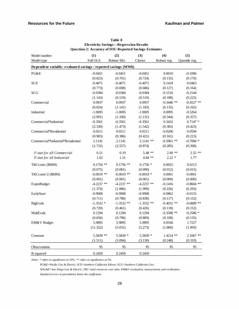
Regression Analysis – Question 2

We ran similar regressions to those displayed above with the IOU accuracy ratios as the dependent variables. As independent variables, we used the same regressors that we used for analyzing Question 1, as well as a quadratic term on program costs, which was added because this additional curvature appears to make a difference in certain regression models. Tables 8 and 9 display the results of the same five regression models, attempting to determine what differentiates an energy-efficiency program that has its IOU-reported savings estimates confirmed by an independent evaluation from one that does not (for both MWh and MW savings). Positive and significant coefficients are indicators of a higher likelihood that the associated regressor is correlated with a greater tendency for third-party evaluations to confirm IOU-reported savings estimates.

From Tables 8 and 9, once again, we see that for some program characteristics, such as IOU service territory, we cannot reject the hypothesis of no effect on the IOU accuracy ratios. Programs that spent a larger percentage of their budgets were more likely to overestimate savings. This may suggest that a higher level of spending provides an additional incentive to the utilities to report a higher level of savings. The size of the program, as captured by program costs, is a positive and significant determinant of the IOU accuracy ratios for the first few regression models, but this effect disappears for the regressions that adjust for outliers.

The most interesting results from Tables 8 and 9 again are the influence of the evaluators. Programs evaluated by Large Firm A or Large Firm B had relatively larger IOU-reported savings estimates compared to the evaluated savings estimates, since the coefficient on “BigEvals” is significantly negative (and large in magnitude). In other words, these evaluators made larger downward corrections of IOU-reported savings estimates than did the smaller and less popular evaluators. This finding could suggest differences in the evaluations themselves more than differences in the programs being evaluated.


28

Table 8Electricity Savings—Regression Results

Question 2: Accuracy of IOU-Reported Savings Estimates


Dependent variable: evaluated savings / reported savings (MWh)

PG&E -0.0451 -0.0451 -0.0451 0.0010 -0.1006(0.823) (0.701) (0.724) (0.135) (0.170)

SCE -0.4071 -0.4071 -0.4071 0.1418 0.0463(0.773) (0.698) (0.686) (0.127) (0.164)

SCG -0.0384 -0.0384 -0.0384 -0.1516 -0.2144(1.143) (0.519) (0.519) (0.188) (0.225)

Commercial 0.0937 0.0937 0.0937 -0.3446 ** -0.4527 **(0.824) (1.141) (1.183) (0.135) (0.165)

Industrial -1.0695 -1.0695 -1.0695 0.0095 -0.5264(2.091) (1.100) (1.131) (0.344) (0.357)

Commercial*Industrial -0.3561 -0.3561 -0.3561 0.3432 0.7147 *(2.330) (1.473) (1.542) (0.383) (0.423)

Commercial*Residential 0.0211 0.0211 0.0211 -0.0206 0.0594(0.983) (0.386) (0.421) (0.161) (0.213)

Commercial*Industrial*Residential 2.1141 2.1141 2.1141 ** -0.5961 ** -0.7084 *(1.732) (2.557) (0.874) (0.285) (0.368)

F-stat for all Commercial 0.51 0.19 5.48 ** 2.90 ** 2.55 ** F-stat for all Industrial 1.02 1.31 4.84 ** 2.22 * 1.77

TRCcosts ($MM) 0.1756 ** 0.1756 ** 0.1756 * 0.0025 0.0213(0.075) (0.081) (0.090) (0.012) (0.015)

TRCcosts^2 ($MM) -0.0019 ** -0.0019 ** -0.0019 * 0.0001 -0.0001(0.001) (0.001) (0.001) (0.000) (0.000)

ExptoBudget -4.2237 ** -4.2237 ** -4.2237 ** -0.1416 -0.8604 **(1.374) (1.886) (1.999) (0.226) (0.293)

EarlyStart -0.9908 -0.9908 -0.9908 -0.0862 -0.0155(0.711) (0.788) (0.838) (0.117) (0.152)

BigEvals -1.3532 * -1.3532 ** -1.3532 ** -0.4031 ** -0.6889 **(0.720) (0.461) (0.426) (0.118) (0.152)

MultEvals 0.1294 0.1294 0.1294 -0.3588 ** -0.2586 *(0.656) (0.796) (0.809) (0.108) (0.135)

EM&V Budget 5.9895 5.9895 5.9895 0.8166 1.7227(11.322) (5.031) (5.273) (1.860) (1.993)

Constant 5.5839 ** 5.5839 * 5.5839 * 1.4214 ** 2.1667 **(1.511) (3.094) (3.130) (0.248) (0.310)


R-squared 0.2450 0.2450 0.2450






29

Table 9Peak Electricity Demand Savings—Regression Results

Question 2: Accuracy of IOU-Reported Savings Estimates


Dependent variable: evaluated savings / reported savings (MW)

PG&E 0.2545 0.2545 0.2545 0.1977 0.0805(0.579) (0.422) (0.449) (0.147) (0.225)

SCE -0.1295 -0.1295 -0.1295 0.2385 * 0.1986(0.549) (0.370) (0.356) (0.140) (0.215)

SCG -0.0060 -0.0060 -0.0060 -0.1000 -0.1328(0.834) (0.410) (0.328) (0.212) (0.330)

Commercial 0.5452 0.5452 0.5452 -0.2767 * -0.4045 *(0.570) (0.465) (0.444) (0.145) (0.223)

Industrial -0.0970 -0.0970 -0.0970 0.1160 -0.6747(1.449) (0.454) (0.472) (0.369) (0.459)

Commercial*Industrial -0.8001 -0.8001 -0.8001 0.2212 1.0963 *(1.657) (0.684) (0.687) (0.422) (0.567)

Commercial*Residential -0.0413 -0.0413 -0.0413 -0.0544 0.0608(0.679) (0.265) (0.261) (0.173) (0.253)

Commercial*Industrial*Residential 1.8719 1.8719 1.8719 ** -0.2381 -0.7849 *(1.250) (2.254) (0.453) (0.318) (0.473)

F-stat for all Commercial 0.85 0.48 5.95 ** 1.21 1.42 F-stat for all Industrial 0.86 0.87 6.40 ** 1.27 1.59

TRCcosts ($MM) 0.1060 * 0.1060 ** 0.1060 ** -0.0226 0.0034(0.056) (0.047) (0.051) (0.014) (0.019)

TRCcosts^2 ($MM) -0.0011 * -0.0011 ** -0.0011 * 0.0005 ** 0.0000(0.001) (0.001) (0.001) (0.000) (0.000)

ExptoBudget -2.7665 ** -2.7665 ** -2.7665 ** 0.3748 -1.1286 **(0.970) (0.954) (1.163) (0.247) (0.391)

EarlyStart -0.1084 -0.1084 -0.1084 -0.1901 -0.1420(0.505) (0.436) (0.423) (0.129) (0.202)

BigEvals -0.9844 * -0.9844 ** -0.9844 ** -0.2360 * -0.6177 **(0.510) (0.291) (0.242) (0.130) (0.209)

MultEvals 0.3968 0.3968 0.3968 -0.0910 -0.1490(0.466) (0.426) (0.388) (0.119) (0.181)

EM&V Budget 4.3071 4.3071 4.3071 -1.1794 -0.2406(7.848) (4.530) (5.124) (1.998) (2.585)

Constant 2.9577 ** 2.9577 ** 2.9577 ** 0.9831 ** 2.5045 **(1.057) (0.848) (0.872) (0.269) (0.428)


R-squared 0.2566 0.2566 0.2566






30

Evaluators—Scatter Plots

Our findings relating to the largest and most frequently used evaluators merit further examination. Those programs evaluated by either Large Firm A or Large Firm B appear to have significantly lower evaluated savings estimates compared to both projected and IOU-reported savings than those programs evaluated by the other contractors. This indicates that either the particular choice of evaluator is an important determinant of how useful the evaluations are or that some unobservable correlated with the evaluator of the program is responsible for these results.

Figure 9 displays individual data points for the IOU accuracy ratios for savings measured in MWh. The chart on left includes all data points, whereas the chart on the right ignores the outlier points and focuses on range in which most of the points are located.

Notes: IOU=investor-owned utility; MWh=megawatt hours.

0%

100%

200%

300%

400%

500%

600%

700%

800%

900%

1000%

1100%

1200%

1300%

1400%

1500%

1600%

1700%

Evaluated to rep

orted savings (M

Wh)

All others Large Firm B Large FirmA

Figure 9.IOU Accuracy Ratios (MWh) by Evaluator

0%

10%

20%

30%

40%

50%

60%

70%

80%

90%

100%

110%

120%

130%

140%

150%

160%

170%

180%

190%

200%

Evaluated to rep

orted savings (M

Wh)

All others Large Firm B Large Firm A


31

Figure 9 is informative in two ways about the distribution of these data. First, the chart on the left shows that the outlier IOU accuracy ratios (for which the evaluated savings is far higher than the IOU-reported savings) are for programs evaluated by the smaller contractors (not Large Firm A or Large Firm B). Second, the chart on the right shows that the outlier programs are not the only source of the difference in IOU accuracy ratios for the different evaluators. The programs evaluated by Large Firm A or Large Firm B have IOU accuracy ratios concentrated most heavily in the range of 30–70 percent, whereas these ratios for the smaller evaluators are more evenly distributed across a much wider range.

Discussion, Limitations, and Conclusions

We have compiled a unique dataset related to the 2004–2005 California utility energy-efficiency program cycle. Along with the characteristics of the specific programs and evaluation processes, our data include three distinct and comparable estimates of energy savings: ex-ante projected savings, ex-post IOU-reported savings, and ex-post third-party evaluated savings. We used these data to analyze how third-party evaluated savings compare to ex-ante projections, as well as what characteristics of the programs and the evaluation process were correlated with success compared to expectations. We also used these data to gauge the benefits of the third-party program evaluations as a check on the incentive of the utilities to overstate energy savings estimates.

We find that most energy-efficiency programs did not meet their energy-savings projections. Also, the IOU-reported savings estimates are systematically higher than the evaluated savings estimates. Interestingly, certain aspects of the evaluation process appear to be a significant determinant of how evaluated savings compare to projections and IOU reported results. In particular, programs evaluated by the largest and most commonly used independent contractors (or an unobservable correlated with this choice) tend to have the lowest evaluated savings estimates.

These results signal to regulators that independent evaluations can be a valuable check on the IOUs ability to make unearned profits and can provide valuable information to future program designers and implementers. However, regulators also need to weigh these benefits against the costs of performing the evaluations.

One limitation of the data used in this paper is that many of the energy-efficiency programs were extremely broad in scope and did not focus on particular customer classes or end uses. This made the process of isolating particular influential features of programs more


32

challenging. Also, while many evaluations are hundreds of pages in length and contain a great deal of detail about the individual programs on which they focused, they contained very different formats and analyses. As a result, comparative analysis is impossible across certain program features or types—such as the use of financial incentives, the level of incentives, and the types of end-uses targeted—and we are unable provide an assessment of how these features of programs affect performance. This severely limits the applicability of these particular results for improving future program designs. To be more useful for future program design, evaluations should catalog information about program features in a standard way across different programs so that the evaluation results can be associated with specific features to facilitate comparative analysis. Such analysis could help program designers target their limited resources to programs that have been proven more effective in producing energy and/or peak load savings. Finally, perhaps the more important limitation of the dataset is the relatively small number observations compared to the amount required to perform a comprehensive analysis of the programs and evaluation processes. For this reason we urge caution in the interpretation of the paper’s results.

Despite these limitations, the 2004–2005 California energy-efficiency program cycle offers a unique opportunity to compare various estimates of energy savings and the associated characteristics of programs and the evaluation process. We are hopeful that our findings will be useful in designing energy-efficiency programs and determining how to use independent third-party program evaluations in the future.


33

References

CPUC (California Public Utilities Commission). 2009a. Energy Efficiency 2006–2007 Verification Report. San Francisco, CA: CPUC, Energy Division.

———. 2009b. Proposed Energy Efficiency Risk Reward Incentive Mechanism. White paper. San Francisco, CA: CPUC, Energy Division.

———. 2009c. Energy Efficiency 2006–2008 Verification Report. San Francisco, CA: CPUC, Energy Division.

———. 2009d. Decision Regarding RRIM Claims for the 2006–2008 Program Cycle. Agenda ID #9048 (Rev. 1).

———. 2007. Interim Opinion on Phase 1 Issues: Shareholder Risk/Reward Incentive Mechanism for Energy Efficiency Programs. Decision 07-09-043.

———. 2004. Administrative Law Judge’s Ruling Clarifying Process for Third Party Energy Efficiency Program Providers to Select Contractor to Carry out Evaluation, Measurement and Verification of 2004-2005 Local Energy Efficiency Programs. Rulemaking 01-08-028.

———. 2003a. Interim Opinion Soliciting 2004–2005 Energy Efficiency Program Proposals and Addressing Scope of Proceeding. Decision 03-08-067.

———. 2003b. Energy Efficiency Policy Manual Version 2. San Francisco, CPUC, Energy Division.

———. 2003c. Interim Opinion Adopting Funding for 2004–2005 Energy Efficiency Programs and Studies. Decision 04-02-59.

———. 2003d. 2004–2005 PGC-Funded Program Budgets and Energy Savings Targets. Attachment 1 to Decision 04-02-059.

California Investor Owned Utilities. 2008. Petition for Modification of Decisions 07-09-043 and 08-01-042 by Pacific Gas and Electric Company (U 39-M), Southern California Edison Company (U 338-E), San Diego Gas & Electric Company (U 902- M), and Southern California Gas Company (U 904-G).

Division of Ratepayer Advocates. 2007. Response of the Division of Ratepayer Advocates to Amended Petition for Modification of Decision 07-09-043 by Pacific Gas and Electric


34

Company, Southern California Edison Company, San Diego Gas & Electric Company and Southern California Gas Company.

Hamilton, Lawrence. 1992. How Robust is Robust Regression? STATA Technical Bulletin 1(2).

IPMVP (International Performance Measurement & Verification Protocol). 2002. Concepts and Options for Determining Energy and Water Savings Volume I. DOE/GO-102002-1554. Oak Ridge, TN: U.S. Department of Energy, Office of Scientific and Technical Information.

National Action Plan for Energy Efficiency. 2008. Vision for 2025: A Framework for Change. Washington, DC: U.S. Environmental Protection Agency.

Snedecor, G.W., and W.G. Cochran. 1967. Statistical Methods. Sixth Edition. Ames, IA: Iowa State University Press, 1967.

TecMarket Works Framework Team. 2004. The California Evaluation Framework. Report prepared for the California Public Utilities Commission and the Project Advisory Group. Oregon, WI: TecMarket Works.

TecMarket Works Team. 2006. California Energy Efficiency Evaluation Protocols: Technical, Methodological, and Reporting Requirements for Evaluation Professionals. Report prepared for the California Public Utilities Commission. San Francisco, CA: CPUC.


35

Appendix

2004–2005 California Energy Efficiency Program Cycle

Program IOU service Customername territory class Primary evaluator

1 ADM Mobile Energy Clinic SDG&E Commercial Sisson and Associates, Inc.2 ADM Mobile Energy Clinic SCE Commercial Sisson and Associates, Inc.3 ADM Mobile Energy Clinic SCG Commercial Sisson and Associates, Inc.4 Appliance Recycling PG&E Residential ADM Associates, Inc.5 Appliance Recycling SDG&E Residential ADM Associates, Inc.6 Appliance Recycling‐Procurement SCE Residential ADM Associates, Inc.7 Appliance Recycling‐Public Goods Charge SCE Residential ADM Associates, Inc.8 California Wastewater Process Optimization PG&E Commercial SBW CONSULTING, INC.9 California Wastewater Process Optimization SDG&E Commercial SBW CONSULTING, INC.10 Comprehensive HTR Mobile Home Program SCG Residential Alternative Energy Systems Consulting11 Comprehensive HTR Mobile Home Program SCE Residential Alternative Energy Systems Consulting12 CUWCC Pre‐Rinse Spray Valve Installation Program PG&E Commercial SBW CONSULTING, INC.13 CUWCC Pre‐Rinse Spray Valve Installation Program SCG Commercial SBW CONSULTING, INC.14 RightLights PG&E Commercial, Industrial Quantec, LLC15 H&L Energy Savers ‐ Performance4 SCE Residential Sisson and Associates, Inc.16 Efficiency on Wheels PG&E Residential, Commericial EMCOR Energy & Technologies17 Small Business Energy Alliance PG&E Commercial Sisson and Associates, Inc.18 Small Business Energy Alliance SCE Commercial Sisson and Associates, Inc.19 QuEST's Building Tune‐Up Program SCE Commercial, Industrial SBW CONSULTING, INC.20 QuEST's Building Tune‐Up Program PG&E Commercial, Industrial SBW CONSULTING, INC.21 Statewide Multifamily Rebate Program PG&E Commercial KEMA22 Statewide Multifamily Rebate Program SDG&E Commercial KEMA23 Statewide Multifamily Rebate Program SCE Commercial KEMA24 Statewide Multifamily Rebate Program SCG Commercial KEMA25 SW‐CAEnergySTAR Homes PG&E Commercial RLW Analytics26 SW‐CAEnergySTAR Homes SCE Commercial RLW Analytics27 SW‐CAEnergySTAR Homes SCG Commercial RLW Analytics28 SW‐CAEnergySTAR Homes SDG&E Commercial RLW Analytics29 Designed for Comfort PG&E Residential, Commericial KEMA30 Designed for Comfort SCE Residential, Commericial KEMA31 Designed for Comfort SCG Residential, Commericial KEMA32 Designed for Comfort SDG&E Residential, Commericial KEMA33 Community EnergyPartnership SCE Residential, Commericial Aloha Systems, Incorporated34 Community EnergyPartnership SCG Residential, Commericial Aloha Systems, Incorporated35 City of Fresno PG&E Residential, Commericial, Industrial ECONorthwest36 Silicon Valley Partnership PG&E Residential, Commericial, Industrial ECONorthwest37 El Dorado County PG&E Residential, Commericial, Industrial ECONorthwest38 City of Stockton PG&E Residential, Commericial, Industrial ECONorthwest39 East Bay Energy Partnership PG&E Residential, Commericial, Industrial ECONorthwest40 Bakersfield Kern Energy Watch Partnership PG&E Residential, Commericial, Industrial ECONorthwest41 Energy Affordability in MF housing PG&E Commercial KEMA42 Energy Solution's PY2004‐2005 LightWash II Program PG&E Residential, Commercial Equipoise Consulting Incorporated43 Non‐Residential Financial Incentives Program SCG Commercial, Industrial ECONorthwest44 Business Energy Services Team Program PG&E Commercial Quantec, LLC45 Business Energy Services Team Program SCE Commercial Quantec, LLC46 Business Energy Services Team Program SCE Commercial Quantec, LLC47 Business Energy Services Team Program SDG&E Commercial Nexant48 Enhanced Automation Intiative PG&E Commercial Quantec, LLC49 Enhanced Automation Intiative SCE Commercial Quantec, LLC50 Energy Smart Grocer SCE Commercial PWP INC.51 Energy Smart Grocer SDG&E Commercial PWP INC.52 Energy Smart Grocer PG&E Commercial PWP INC.53 San Diego Region Local Government Energy Efficiency Program SDG&E Commercial Nexant54 Shade Tree Program SDG&E Residential Zebedee & Associates55 Residential Duct Services SCE Residential NA56 Residential Duct Services SCG Residential NA57 Local Nonresidential Sustainable Communities SDG&E Commercial Quantec, LLC58 City of Pomona Partnership SCE NA Quantec, LLC59 Small Business Energy Efficiency SDG&E Commercial ECONorthwest


36

Notes: IOU=investor-owned utility; PG&E=Pacific Gas & Electric; SCE=Southern California Edison; SCG=Southern California Gas; SDG&E=San Diego Gas & Electric.

2004–2005 California Energy Efficiency Program Cycle

Program IOU service Customername territory class Primary evaluator

60 California Multi‐measure Farm Program PG&E Commercial kW Engineering61 California Multi‐measure Farm Program SCE Commercial kW Engineering62 HTR Lighting Turn‐in SDG&E Residential Itron, Inc.63 Limited Income Refrigerator Replacement & Lighting SDG&E Residential Quantec, LLC64 Retrocommissioning Program SDG&E Commercial Itron, Inc.65 RCA Verification Program for Residential and Commercial Air Conditioners SCE Residential, Commercial Aloha Systems, Incorporated66 RCA Verification Program for Residential and Commercial Air Conditioners PG&E Residential, Commercial Aloha Systems, Incorporated67 RCA Verification Program for Residential and Commercial Air Conditioners SDG&E Residential, Commercial Aloha Systems, Incorporated68 Emerging Communities Energy Efficiency Program (ECEEP) SCE Commercial Robert Mowris & Associates69 California Irrigation Technology Agricultural Pumping Efficiency Program PG&E Industrial, Commercial Equipoise Consulting Incorporated70 California Irrigation Technology Agricultural Pumping Efficiency Program SCG Industrial, Commercial Equipoise Consulting Incorporated71 California Irrigation Technology Agricultural Pumping Efficiency Program SCE Industrial, Commercial Equipoise Consulting Incorporated72 City of Berkeley CA Youth Energy Services Program PG&E Residential Summit Blue Consulting, LLC73 Certified Agri‐Food Energy Efficiency PG&E Industrial Quantec, LLC74 Compressed Air Management Program PG&E Industrial Ridge & Associates75 CSU/IOU Partnership SDG&E Commercial SBW CONSULTING, INC.76 CSU/IOU Partnership PG&E Commercial SBW CONSULTING, INC.77 CSU/IOU Partnership SCE Commercial SBW CONSULTING, INC.78 CSU/IOU Partnership SCG Commercial SBW CONSULTING, INC.79 Express Efficiency PG&E Commercial, Industrial Itron, Inc.80 Express Efficiency SCG Commercial, Industrial Itron, Inc.81 Express Efficiency SDG&E Commercial, Industrial Itron, Inc.82 Express Efficiency ‐ Procurement SCE Commercial, Industrial Itron, Inc.83 Express Efficiency ‐ Procurement PG&E Commercial, Industrial Itron, Inc.84 Express Efficiency ‐ Public Goods Charge SCE Commercial, Industrial Itron, Inc.85 Integrated Audits PG&E Commercial, Industrial Itron, Inc.86 LA County Partnership SCE Commercial RLW Analytics, Inc.87 LA County Partnership SCG Commercial RLW Analytics, Inc.88 Local Nonresidential Customer Energy Savings Bid SDG&E Commercial, Industrial KEMA89 Local Nonresidential Energy Saver SDG&E Commercial Quantec, LLC90 Moderate Income Comprehensive Attic PG&E Residential Robert Mowris & Associates91 Nonresidential Energy Audits PG&E Commercial, Industrial Itron, Inc.92 Nonresidential Energy Audits SCE Commercial, Industrial Itron, Inc.93 Nonresidential Energy Audits SDG&E Commercial, Industrial Itron, Inc.94 Nonresidential Energy Audits SCG Commercial, Industrial Itron, Inc.95 Rebuild a Greener San Diego SDG&E Residential Zebedee & Associates96 San Diego City Schools Retrofit Partnership SDG&E Commercial KEMA97 San Francisco Peak Pilot PG&E NA Summit Blue Consulting, LLC98 Savings By Design PG&E Commercial, Industrial RLW Analytics99 Savings By Design SCE Commercial, Industrial RLW Analytics100 Savings By Design SCG Commercial, Industrial RLW Analytics101 Savings By Design SDG&E Commercial, Industrial RLW Analytics102 Single‐Family EE Rebates PG&E Residential Itron, Inc.103 Single‐Family EE Rebates SCE Residential Itron, Inc.104 Single‐Family EE Rebates SCG Residential Itron, Inc.105 Single‐Family EE Rebates SDG&E Residential Itron, Inc.106 Small Non‐residential Energy Fitness Program PG&E Commercial Robert Mowris & Associates107 Small Nonresidential Hard to Reach Program SCE Commercial ECONorthwest108 Standard Performance Contract PG&E Commercial, Industrial Itron, Inc.109 Standard Performance Contract SCE Commercial, Industrial Itron, Inc.110 Standard Performance Contract SDG&E Commercial, Industrial Itron, Inc.111 Upstream HVAC and Motors PG&E Commercial, Industrial Itron, Inc.112 Upstream HVAC and Motors SCE Commercial, Industrial Itron, Inc.113 Upstream HVAC and Motors SDG&E Commercial, Industrial Itron, Inc.114 Upstream HVAC and Motors ‐ Procurement PG&E Commercial, Industrial Itron, Inc.115 Ventura REA SCE NA NA116 Ventura REA SCG NA NA117 VeSM SCE NA NA118 Yolo Energy Efficiency Project PG&E Residential, Commercial HESCHONG MAHONE GROUP, INC.

april 2010 rff dp 10-16 discussion paper · april 2010 rff dp 10-16 energy-efficiency ... excluded...

Documents