january 2009 rff dp 08-46 discussion paper

1616 P St. NW Washington, DC 20036 202-328-5000 www.rff.org

January 2009 RFF DP 08-46

Optimal Energy Efficiency Policies and Regulatory Demand-Side Management Tests

How Well Do They Match?

T im Bren nan

DIS

CU

SSIO

N P

APE

R

© 2009 Resources for the Future. All rights reserved. No portion of this paper may be reproduced without permission of the authors.

Discussion papers are research materials circulated by their authors for purposes of information and discussion. They have not necessarily undergone formal peer review.

Optimal Energy Efficiency Policies and Regulatory Demand-Side Management Tests: How Well Do They Match?

Tim Brennan

Abstract Under conventional models, subsidizing energy efficiency requires electricity to be priced below

marginal cost. Its benefits increase when electricity prices increase to finance the subsidy. With high prices, subsidies are counterproductive unless consumers fail to make efficiency investments when private benefits exceed costs. If the gain from adopting efficiency is only reduced electricity spending, capping revenues from energy sales may induce a utility to substitute efficiency for generation when the former is less costly. This goes beyond standard “decoupling” of distribution revenues from sales, requiring complex energy price regulation. The models’ results are used to evaluate tests in the 2002 California Standard Practice Manual for assessing demand-side management programs. Its “Ratepayer Impact Measure” test best conforms to the condition that electricity price is too low. Its “Total Resource Cost” and “Societal Cost” tests resemble the condition for expanded decoupling. No test incorporates optimality conditions apart from consumer choice failure.

Key Words: Electricity, energy efficiency, demand-side management, utility regulation, decoupling

JEL Classification Numbers: L94, L51, Q48

Contents

1. Introduction ........................................................................................................................ 1

2. Optimal Efficiency Subsidy Models ................................................................................. 4

2.1. Simple Efficiency Subsidy Modeling ......................................................................... 4

2.2. Paying for the Subsidy through Higher Electricity Prices .......................................... 8

2.3. Consumer Choice Failure ......................................................................................... 10

2.4. Consumer Choice Failure with Endogenous Subsidy Cost ...................................... 16

2.5. Consolidating the Conditions .................................................................................... 20

3. Comparisons to the California Manual ......................................................................... 22

3.1. Useful Simplifications .............................................................................................. 22

3.2. General Shortcomings of the Tests ........................................................................... 24

3.3. Description and Assessment ..................................................................................... 26

4. Conclusions ....................................................................................................................... 30

References .............................................................................................................................. 32

Resources for the Future Brennan

1

Optimal Energy Efficiency Policies and Regulatory Demand-Side Management Tests: How Well Do They Match?

Tim Brennan∗

1. Introduction

Interest in electricity conservation is increasing for at least four reasons: greenhouse gas concern, excessive use on-peak due to the absence of real-time pricing, the economic and political costs of expanding transmission and generation capacity, and a widespread belief that consumers fail to invest in privately cost-effective, energy-efficient technologies because of limits in information (such as not having information on net benefits) or cognition (not being able to translate that information into welfare-maximizing choices). The latter is particularly consequential because it cannot be addressed simply by adopting rules or institutions that “set the right prices,” e.g., by incorporating marginal costs of environmental externalities through cap-and-trade programs or expanding the use of smart meters, real-time price information, and automated controls that allow time-variant pricing and provide missing incentives to use energy more efficiently.

This interest has manifestations on two fronts. On the modeling side, the challenge has been to identify optimum conditions for subsidizing investments in energy, recognizing all of these characteristics, including consumer choice failure.1 Brennan (2008a) sets out a model producing such conditions; this model serves as the basis for the analysis here. To deal with consumer choices failure, we portray welfare effects of subsidizing efficiency by assigning the full welfare benefits of those investments through expansion of the set of individuals who are induced to act rationally by the subsidies. Such an ascription is inconsistent with basing welfare on revealed preference, but the inconsistency is an inevitable consequence of assuming that consumers fail to act in their self-interest by under-investing in efficiency.

We will see that consumer choice failure is necessary for subsidies to be warranted when electricity prices are too high. In Maryland, likely a typical example, electricity policy concern

∗ Professor, Public Policy and Economics, University of Maryland, Baltimore County; Senior Fellow, Resources for the Future. Email: [email protected]. Much of the discussion of the efficiency model in Sections 2.3.1 and 2.3.2 draws from pp. 16-20 of Brennan (2008a). 1 Sanstad and Howarth (1994) provide a useful survey of the debate.


2

rest on two principles—people purchase too much electricity, and its price is too high. For example, the opening sentence of the Maryland Energy Administration’s Strategic Electricity Plan states

Over the last year, Maryland experienced dramatic hikes in electricity bills, warnings of summer time electricity shortages as early as 2011, and growing concern about the potential impact of climate change (MEA, 2008 at 1).

The sentence opens with the idea that prices are excessive, and then warns that demand will exceed supply and that electricity use should be cut to mitigate climate change. This paradoxical juxtaposition is quite common, particularly in states where residential rates have dramatically risen following the expiration of regulations that fixed prices for a time period following the initial opening of retail markets to competition.2 With conventional models of consumer choice, where purchases are made up to the point where marginal willingness to pay equals price, excessive consumption implies that the price the consumer faces is too low—below marginal cost, and should be higher, not lower. The only way to reconcile excessive consumption with prices being too high is consumer choice failure.

At the same time, state electricity regulators, while encouraging utilities to support demand-side management programs, have to ensure that the benefits of those programs justify their costs. Since 2002, the primary method for doing so involves the application of a number of tests initially proposed in a California Standard Practice Manual (State of California, 2002, hereafter referred to as “California Manual”). That manual includes four tests based nominally on net revenue benefits to consumers (“Participant test”), effects on utility bills (“Ratepayer Impact Measure test”), net costs to ratepayers and utilities (“Total Resource Cost test”), and net costs of the program itself (“Program Administrator Cost test”). The Total Resource Cost test is amended in some jurisdictions to include externality costs, thus becoming a “Societal Cost test”.

The purpose of this paper is to develop optimality conditions for efficiency subsidies and translate these tests into terms that facilitate using these conditions to evaluate the theoretical foundations of the tests. The following section of the paper sets out an optimal efficiency subsidies model, in four steps. The first step identifies the basic model for energy subsidies; the

2 Martin O’Malley, the current governor of Maryland who has proposed an “EmPower Maryland” to program reduce per capita electricity use 15% by 2015 (MEA, 2008 at 21), campaigned on a platform emphasizing that consumers were paying too much for electricity. See his campaign’s online article, “Defending Maryland Against Rising Energy Prices,” http://www.martinomalley.com/content/591, accessed July 29, 2008.


3

case rests, not surprisingly, on an argument that the price of electricity is too low.3 This can result from energy prices not reflecting external costs, e.g., related to fossil fuel emissions, or inability of prices to track variation in real-time costs due to variation in demand relative to capacity (Brennan, 2004). The second step extends the model by having the subsidy funded through electricity surcharges. If prices are too low, then the subsidy has the additional benefit of increasing price to get it closer to the optimal level.4

In the third step, we drop explicit treatment of the funding question and instead incorporate a welfare effect based on using subsidies as an instrument to get consumers to adopt energy efficiency technologies that they find privately beneficial. Such considerations do not lend themselves to standard economic modeling, because revealed preference not to purchase energy efficiency is mistrusted as an indicator of underlying consumer welfare. We assume that the subsidy acts like information, in that making efficiency investments less expensive induces more consumption, and once consumed, those investments produce net economic benefit as if those benefits had been recognized all along. Since utility efficiency programs are defended largely on their ability to induce consumers to appreciate the private benefits of energy efficiency, a model needs to try to represent these benefits. Without such a representation, the programs would be unjustified unless inappropriately low energy prices were inducing inefficiently large levels of use.

The fourth step combines the analyses in the previous two steps into a model in which ratepayers as a whole cover the cost of efficiency subsides justified in part as overcoming some consumers’ error in not making efficiency investments on their own. To assess the California Manual tests for evaluating utility programs, the theoretical model used as the basis for comparison needs to reflect the method of funding—increasing utility rates to cover the cost of the subsidies—and the rationale to overcome consumer error in not making energy investments. We also will need to incorporate an administrative cost to the utility of managing the subsidy program. This second section concludes with an application of the model to policies to decouple revenues from sales in the electricity sector. Assuming consumers irrationally refuse to invest in energy efficiency, this model supports a more radical conception of decoupling, making revenues

3 Brennan (1998) offered an earlier version of this argument in assessing demand-side management programs. 4 Similar considerations can justify the imposition of reserve requirements, if doing so leads to higher prices by internalizing the “blackout externality,” i.e., when my use of electricity increases stresses on the overall grid and thus your chance of suffering an outage (Brennan, 2008b).


4

from energy sales, and not just those from distribution fees, independent of the amount of electricity consumers use.

The third section of the paper translates the five proposed tests in the California Manual into the terms of these models. It begins with simplifications needed to match the marginal optimality conditions to the gross benefits and costs the California Manual compares. After presenting some generic shortcomings of the tests, we follow with an assessment of how they conform to the recommendations of the model. The fourth section of the paper offers conclusions and caveats.

2. Optimal Efficiency Subsidy Models

2.1. Simple Efficiency Subsidy Modeling

The interest by regulators, consumers, environmentalists, conservationists, and utilities in energy efficiency programs, and specifically in whether the California Manual tests for when such programs should be accepted by regulators, leads us to investigate when such subsidies would be warranted. We begin with what may be the simplest model to begin to answer that question. We begin with a demand function Q(p, x) for electricity, where Q is quantity demanded at price p and with electricity efficiency purchases x. We assume that Qp < 0.

The sign of Qx depends on p and x. The expectation is that it is negative over prevailing prices. Were it negative over all prices, then increasing x would reduce Q for all p, causing the gross consumer surplus of electricity use at any price or quantity to decline, as in Figure 1a. This would contradict the idea that efficiency investments provide more benefit from using less electricity. Moreover, if consumer surplus did not increase with efficiency investments over some range, the conservationists’ claim that consumers would really be better off with these investments, because the cost of the electricity saved is less than the cost of the investment, would be specious. Accordingly, the effect of increasing x on the demand curve for electricity is more like pivoting it around some point, where surplus from the initial amount consumes increases, but beyond some quantity the marginal willingness to pay falls, as in Figure 1b.


5

Figure 1a Figure 1b

We will allow consumer surplus from electricity use to increase with x, to have at least some efficiency purchases in the absence of policy interventions, but will also assume that we are in the range of prices where Qx < 0.5

To analyze the effects of efficiency investments, we also define the following: Let pr be the retail price of electricity. For simplicity, we assume that pr is set exogenously, either through price-cap regulation or lagged rate-of-return regulation of the energy sales by incumbent distribution utilities. Another possibility, neither assumed elsewhere nor realistic, would be that the marginal cost of supply is constant; a more reasonable assumption would be the inability to institute real-time pricing that would allow prices to track marginal cost. Because we are

5 It is well known that energy subsidies can reduce demand for energy at price pr, yet increase surplus by increasing the value of inframarginal consumption. As Figure 1b illustrates, to have consumer surplus increase with energy efficiency, Qx(pr, x) will be positive for high prices, displaying the so-called “rebound effect” (Gottron [2001] attributes the idea to Stanley Jevons in 1865.) The conditions for the rebound effect can be illustrated as follows: Define an efficiency level k as when an appliance delivers k units of service for each unit of energy it uses. At an energy price p, the cost of each unit of service delivered is p/k. The total amount of energy consumed, e, then will be Q(p/k)/k. de/dk = –Q/k2 – pQ'/k3. This expression will be positive if – [p/k][Q'/Q] > 1, i.e., the demand for the energy services is elastic. If there are other marginal usage costs apart from energy, such as wear-and-tear, the elasticity required for increased efficiency to increase energy use is greater. As Figure 1b shows, for efficiency investments to benefit consumers, there must be prices at which the rebound effect would hold.

Q(p, x)

Q

p

Q(p, x + dx)

Q(p, x)

Q(p, x)

Q

p

Q(p, x + dx)


6

examining contexts in which regulators are considering whether efficiency programs warrant increases in regulated rates, assuming price regulation seems reasonable. 6 It may be more of a stretch to assume exogenous pricing of electricity, rather than the price being set endogenously as the average cost of providing Q units of electricity. However, assuming exogenous energy prices allows one to avoid complexities in the modeling, without impeding our ability to assess the California Manual tests.

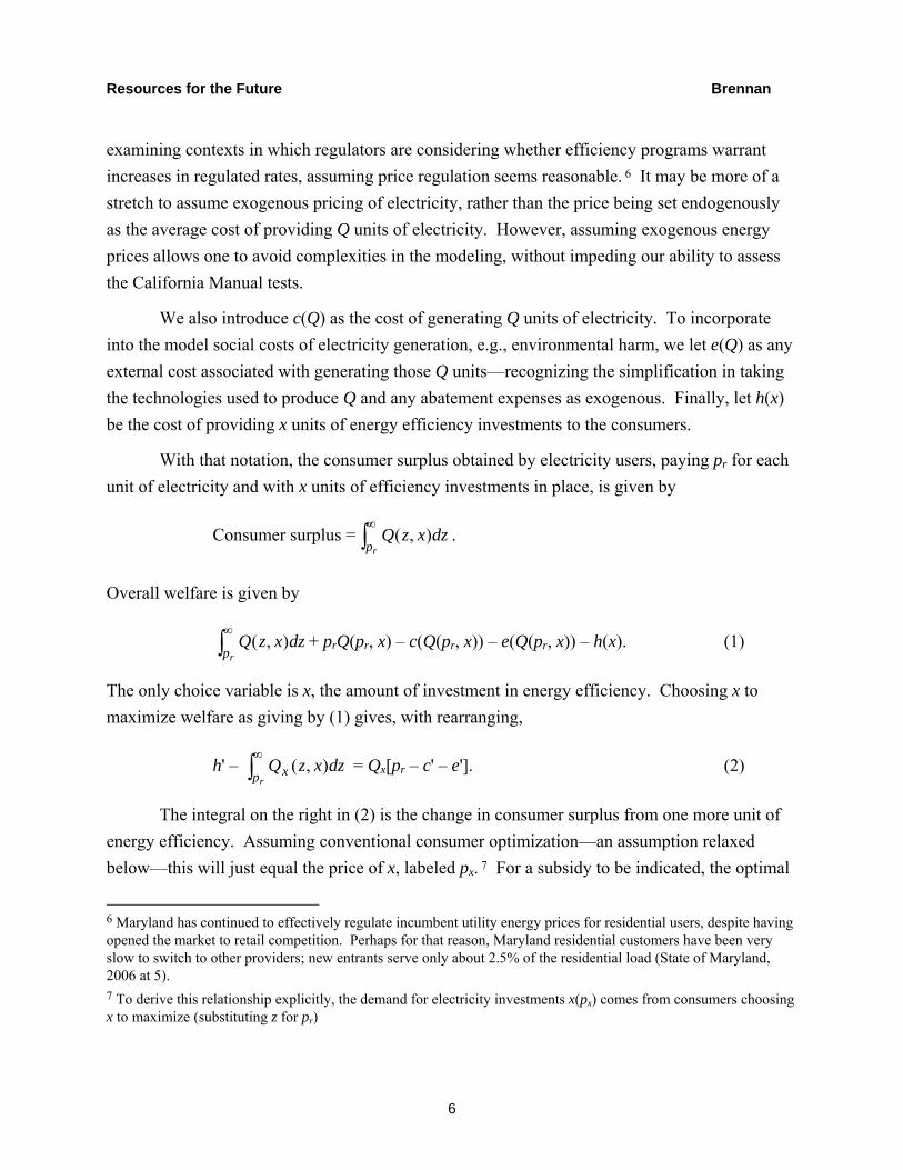
We also introduce c(Q) as the cost of generating Q units of electricity. To incorporate into the model social costs of electricity generation, e.g., environmental harm, we let e(Q) as any external cost associated with generating those Q units—recognizing the simplification in taking the technologies used to produce Q and any abatement expenses as exogenous. Finally, let h(x) be the cost of providing x units of energy efficiency investments to the consumers.

With that notation, the consumer surplus obtained by electricity users, paying pr for each unit of electricity and with x units of efficiency investments in place, is given by

Consumer surplus = ∫∞

rpdzxzQ ),( .

Overall welfare is given by

∫∞

rpdzxzQ ),( + prQ(pr, x) – c(Q(pr, x)) – e(Q(pr, x)) – h(x). (1)

The only choice variable is x, the amount of investment in energy efficiency. Choosing x to maximize welfare as giving by (1) gives, with rearranging,

h' – ∫∞

rp x dzxzQ ),( = Qx[pr – c' – e']. (2)

The integral on the right in (2) is the change in consumer surplus from one more unit of energy efficiency. Assuming conventional consumer optimization—an assumption relaxed below—this will just equal the price of x, labeled px. 7 For a subsidy to be indicated, the optimal

6 Maryland has continued to effectively regulate incumbent utility energy prices for residential users, despite having opened the market to retail competition. Perhaps for that reason, Maryland residential customers have been very slow to switch to other providers; new entrants serve only about 2.5% of the residential load (State of Maryland, 2006 at 5). 7 To derive this relationship explicitly, the demand for electricity investments x(px) comes from consumers choosing x to maximize (substituting z for pr)


7

price must be below marginal cost, i.e., px less than h', making the left-hand side of (2) positive. With Qx negative, a necessary condition for a subsidy is

pr < c' – e'.

The price of electricity must be below its marginal production cost plus any marginal external cost associated with its generation or use. This is not surprising, as it is just an example of the “theory of the second best” (Lipsey and Lancaster, 1956). If the price of one product is below its marginal cost—here electricity—one would want to subsidize substitutes—here, energy efficiency.

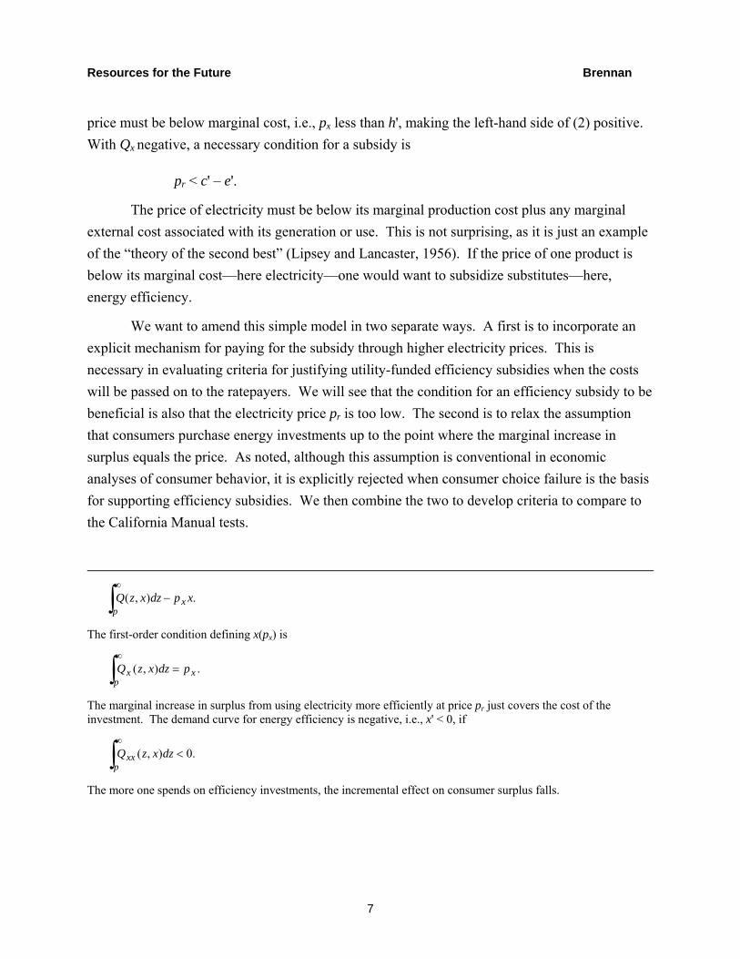
We want to amend this simple model in two separate ways. A first is to incorporate an explicit mechanism for paying for the subsidy through higher electricity prices. This is necessary in evaluating criteria for justifying utility-funded efficiency subsidies when the costs will be passed on to the ratepayers. We will see that the condition for an efficiency subsidy to be beneficial is also that the electricity price pr is too low. The second is to relax the assumption that consumers purchase energy investments up to the point where the marginal increase in surplus equals the price. As noted, although this assumption is conventional in economic analyses of consumer behavior, it is explicitly rejected when consumer choice failure is the basis for supporting efficiency subsidies. We then combine the two to develop criteria to compare to the California Manual tests.

∫∞

−p

x xpdzxzQ .),(

The first-order condition defining x(px) is

∫∞

=p

xx pdzxzQ .),(

The marginal increase in surplus from using electricity more efficiently at price pr just covers the cost of the investment. The demand curve for energy efficiency is negative, i.e., x' < 0, if

∫∞

<p

xx dzxzQ .0),(

The more one spends on efficiency investments, the incremental effect on consumer surplus falls.


8

2.2. Paying for the Subsidy through Higher Electricity Prices

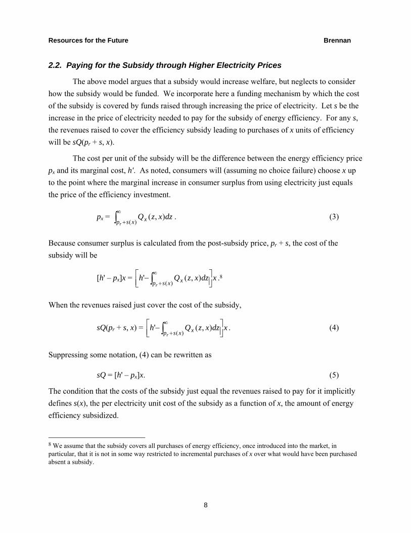
The above model argues that a subsidy would increase welfare, but neglects to consider how the subsidy would be funded. We incorporate here a funding mechanism by which the cost of the subsidy is covered by funds raised through increasing the price of electricity. Let s be the increase in the price of electricity needed to pay for the subsidy of energy efficiency. For any s, the revenues raised to cover the efficiency subsidy leading to purchases of x units of efficiency will be sQ(pr + s, x).

The cost per unit of the subsidy will be the difference between the energy efficiency price px and its marginal cost, h'. As noted, consumers will (assuming no choice failure) choose x up to the point where the marginal increase in consumer surplus from using electricity just equals the price of the efficiency investment.

px = ∫∞

+ )(),(

xsp xr

dzxzQ . (3)

Because consumer surplus is calculated from the post-subsidy price, pr + s, the cost of the subsidy will be

[h' – px]x = xdzxzQhxsp x

r ⎥⎦⎤

⎢⎣⎡ −∫

∞

+ )(),(' .8

When the revenues raised just cover the cost of the subsidy,

sQ(pr + s, x) = xdzxzQhxsp x

r ⎥⎦⎤

⎢⎣⎡ −∫

∞

+ )(),(' . (4)

Suppressing some notation, (4) can be rewritten as

sQ = [h' – px]x. (5)

The condition that the costs of the subsidy just equal the revenues raised to pay for it implicitly defines s(x), the per electricity unit cost of the subsidy as a function of x, the amount of energy efficiency subsidized.

8 We assume that the subsidy covers all purchases of energy efficiency, once introduced into the market, in particular, that it is not in some way restricted to incremental purchases of x over what would have been purchased absent a subsidy.


9

Welfare as a function of x with the subsidy endogenously determined by (5) is given by amending (1) to include s(x):

∫∞

+ )(),(

xsprdzxzQ + [pr+s(x)]Q(pr+s(x), x) – c(Q(pr+s(x), x)) – e(Q(pr+s(x), x)) – h(x). (6)

From (6), the marginal effect of increasing x on welfare, with the endogenous subsidy cost, is given by

[px – h'] + [pr + s – c' – e'][Qps' + Qx],9 (7)

Let x* be the amount of energy efficiency purchased with no subsidy, i.e., s(x*) = 0. We take s'(x*) > 0, consistent with assuming that electricity and energy efficiency are substitutes at the margin; increasing the price of electricity is consistent with increasing the amount of energy efficiency consumed.10 A subsidy is warranted if (7) is positive at x*. At x*, px = h', so the first term in (5) is zero. If s(x*) is also zero, a subsidy is warranted if

[pr – c' – e'][Qps' + Qx] > 0. (8)

Assuming as before that at the margin energy efficiency investments reduce electricity use, Qx is negative. Qps' is negative as well, because s' is positive and Qp is negative.

As in the basic case, a subsidy is warranted only if the first bracketed term is negative. The retail price of electricity has to be below its marginal cost of production plus any marginal external cost, i.e., pr is less than c' + e'. However, unlike the base case, increasing the use of energy efficiency has two benefits. The first, from the Qx term, is as before—reducing the use of electricity, which is consumed more than is socially optimal because the price is too low. The second effect comes from Qps' being negative. This benefit is that increasing the use of energy

9 The term s'(x)Q(pr + s(x), x) arises both in the negative, in the differentiation of the integral, and in the positive, in the differentiation of [pr + s(x)]Q(pr + s(x), x), and thus cancels, leaving (7). 10 This does not follow solely from (5). Increasing x both increases the cost of the subsidy and thus, the revenue required. In the relevant range, demand for electricity is likely to be sufficiently inelastic that increasing s increases the revenue generated to pay for the subsidy. Moreover, by reducing the amount of electricity used, increasing x directly increases the per-electricity electricity premium s needed to cover the cost of the subsidy. Finally, we assume that holding x constant, the reduced demand for electricity implies that consumers are shedding load for which the marginal willingness to pay falls as electricity use increases—this is the basis for regarding efficiency investments as a substitutes for electricity use rather than complement at the margin. Increasing s increases the price consumers would pay for efficiency holding x constant, and thus reduces the cost of the subsidy, allowing for more x to be subsidized. For more detail, see the derivation in Section 2.4.1.


10

efficiency above the optimum, by raising the price of electricity by s' reduces electricity use by Qps'. That benefit would be present even if the subsidy were not used to fund energy efficiency investments.

2.3. Consumer Choice Failure

2.3.1. Assigning and Calculating Consumer Surplus

We temporarily turn aside from endogenous subsidies to focus on the idea that subsidies not only induce people who are purchasing energy efficiency to purchase more, but also lead people to make energy-efficiency purchases who had not been doing so despite the benefit they would have gotten. As noted, this reflects a widespread assumption among energy efficiency advocates that consumers would be better off making these investments but fail to do so because of incomplete information or inability to translate that information into beneficial action. This perspective runs counter to the economically conventional assumption that choices reveal preferences; here some people are not choosing to make efficiency investments but, by their own lights, would be better off having done so. Accordingly, whether consumer choice failure exists is something many may reasonably doubt; any such doubt will not be confronted or resolved here.

Consumer choice failure turns out to be necessary to resolve the inconsistency between the claims that consumers use too much electricity and that the price of electricity is too high. Incorporating it requires identifying different types of consumers, those who make energy efficiency investments on their own, and those who do not. We do not explicitly model the process by which consumer choice failures might be overcome for the latter group, but assume simply that the lower the price of energy efficiency, px, the greater will be the fraction of consumers that overcome choice failures that defer purchasing any at all. We assume a continuum of consumers, indexed along the line from 0 to 1. Each has the same demand for electricity, given levels of efficiency investments. Portraying consumers as otherwise identical reflects the view that such investments are equally beneficial to all.

The only difference among the consumers is that only a fraction t(px) between 0 and 1 purchases energy efficiency investments at px. Because of cognitive limitations or insufficient information, a fraction of 1 – t(px) does not bother to take advantage of those investments. To model the belief that a subsidy induces not only more energy efficiency by those who already were making the “right” choices, but that it also induces more people to make those choices at all, we assume t' ≤ 0; the lower the price of energy efficiency, the greater the fraction of


11

consumers that will choose to take advantage of efficiency investments. Again, to be clear, the increase is not because consumers previously on the margin now find efficiency worthwhile; it is that the lower price somehow leads them to realize that efficiency investments were worthwhile all along.

As before, let pr be the exogenous retail price of electricity. To represent the effect of overcome alleged choice failure, let px rather than x be the policy instrument. We let x(px) be the amount of efficiency equipment or investment purchased by the t(px) fraction of consumers aware of efficiency benefits at px. The consumer surplus of the fraction that makes these purchases will be

,))(,()( ∫∞

rp xx dzpxzQpt (9)

The similar expression for the surplus for those who do not purchase any energy efficiency, i.e., with x being zero, is

[ ] .)0,()(1 ∫∞

−rpx dzzQpt (10)

The total quantity of electricity demanded when efficiency investments are priced at px, labeled D(px), is

D(px) = t(px)Q(pr, x(px)) + [1 – t(px)]Q(pr, 0). (11)

The profits of selling this electricity at price pr are

pr[D(px)] – c(D(px)).11 (12)

The externality cost at the quantity of electricity chosen will be

e(D(px)). (13)

To complete the model, we include the cost of providing the efficiency investments consumers purchase, t(px)x(px), which is

11 Because surplus for efficiency is based on quantity, not price, we need only subtract the cost of providing the level of energy efficiency investment.


12

h(t(px)x(px)). (14)

The monetary cost of the subsidy is

[h' – px]t(px)x(px). (15)

For now we neglect the costs of raising the funds to cover the subsidy. For purposes of comparison with the California Manual, we model raising the funds through higher electricity prices as in the previous section.12

We thus choose px to maximize welfare W(px), given by the sum of the consumer surpluses from the efficiency-using and non-efficiency using consumers in (9) and (10), plus profits as defined in (12), less external costs as modeled in (13) and efficiency production costs as modeled in (14). The derivative of W with respect to px is:

⎥⎦⎤

⎢⎣⎡ −+ ∫∫∫

∞∞∞dzzQdzxzQtdzxzQtx

rrr ppp x )0,(),('),('

]''[')]]0,(),(['),('][''[ xttxhpQxpQtxpQtxecp rrrxr +−−+−−+ . (16)

The first term is the change in consumer surplus from those who had adopted energy efficiency and increased their efficiency investments. The second is the change in consumer surplus arising from the consumers who, as a result of the lower price, overcome choice failure to adopt energy efficiency. The third term is the change in electricity profits and external costs from the reduction in electricity use when the price of energy efficiency falls, both from those who had adopted and change the amount of efficiency investments marginally, and the change in use from those who jump the fence from non-users to users. The last term is the change in the cost of providing energy efficiency, both to those who had been using it and those who newly adopt.

2.3.2. Analysis of Conditions

It is useful to collect terms in (16) by whether the effect is driven by the change in energy efficiency from those who are already purchasing it (tx'), and whether the effect is driven by the change in those who consume energy efficiency at all (t'). The first set of terms, corresponding to those who had been consuming energy efficiency is

12 Were the subsidy paid for out of general revenues, then one would want to include as a cost the burden of the taxes associated with raising the funds to cover these subsidies.


13

⎥⎦⎤

⎢⎣⎡ −+−− ∫

∞'),(),(]''[' hdzxzQxpQecptx

rp xrxr , (17)

and the second set, corresponding to the effect of overcoming choice failure through efficiency subsidies, is:

⎥⎦⎤

⎢⎣⎡ −⎥⎦

⎤⎢⎣⎡ −+−−− ∫∫

∞∞xhdzzQdzxzQpQxpQecpt

rr pprrr ')0,(),()]0,(),(][''[' . (18)

Consider first the effect as described in (17) on those who are already making energy efficiency investments. This effect is similar to that described above for subsidies. If the electricity price pr equals the sum of marginal production cost c' and marginal externality cost e', the first term is zero.13 If efficiency investments are priced at their marginal cost, h', the sum of the last two terms is zero because the integral, the marginal benefit of making an additional investment in energy efficiency, just equals px. From (17) alone, the case for a subsidy would depend on the expression inside the brackets equaling zero, and this will hold with prices below marginal cost only if pr < c' + e'.14 Demand-reduction subsidies are efficient if and only if prices are too low—less than marginal production and externality cost.

This result need not hold if one takes into account an effect of subsidies on getting more consumers to invest in energy efficiency, when the benefits to those consumers exceed the costs but have not yet made such investments.15 To understand the effect of mitigating consumer choice failure as described in (18), let ΔQ be the effect on electricity usage at price pr when a customer switches from no energy efficiency to making investments at px:

ΔQ = Q(pr, x(px)) – Q(pr, 0). (19)

13 The cost faced by the distribution utility is the wholesale price. We do not distinguish here between short-run and long-run marginal generation costs in setting that price. Overall, wholesale prices of electricity should be high enough not just to cover short run fuel and operating costs but the costs of the generation capacity used to produce that electricity (Brennan 2006). 14 Recall that Qx(pr, x) is assumed to be negative. 15 We neglect a possible monopsony effect. One consumer’s reduction in demand may benefit other consumers by reducing the quantity of electricity needed to meet demand and thus its price. Depressing price through the exercise of market power may increase the economic welfare of consumers, but not necessarily the overall economic performance of the energy sector.


14

We take ΔQ < 0; those who make energy investments use less electricity. For consumers who make the switch, the increase in consumer surplus from overcoming choice failure and realizing the benefits of efficiency investments would be ΔCS,

.)0,(),( dzzQdzxzQCSrr pp ∫∫∞∞

−=Δ (20)

With these abbreviations and suppressing some notation, (18) becomes

t'[[pr – c' – e']ΔQ + ΔCS – h'x]. (21)

Assuming energy efficiency investments are beneficial if priced at marginal cost, we have that ΔCS > h'x when px = h'(x(px)). Because t' ≤ 0, i.e., reducing price leads to more consumers adopting energy investments, we have from (21) that overall economic welfare would increase from a reduction in price from this effect alone, by leading more consumers to act in their own interest.

Because ΔQ is negative, the first term inside the brackets in (21) is positive if and only if pr is less than the sum of c' and e'. If the retail price of electricity is too low in this sense, the effect of too much consumption for that reason reinforces the effect of too much consumption because of consumer choice failure. This strengthens the case for subsidizing efficiency to reduce px below marginal cost. However, even if the electricity price is above marginal production and externality cost, (21) can still be negative. It may still be beneficial to induce more consumers to adopt energy efficiency even if the price is too high. If the fraction of consumers led to increase efficiency use as a result of the subsidy (|t'|) is sufficiently large, and the number who have no choice failure and are consuming electricity already (t) is sufficiently small, then an efficiency subsidy can be beneficial, even if the price of electricity is too high and, all else equal, people are consuming too little electricity.16 Consumer choice failure can justify subsidies even when the price is too high.

2.3.3. Decoupling Implications

Before incorporating the cost of any subsidies, an additional consequence of (21) merits some attention. Assume that the amount of electricity services a consumer “consumes”—light, cooling, refrigeration, heating, communication—is the same regardless of energy efficiency

16 It may help the intuition to note that the same result obtains if marginal production or externality costs are smaller. Either reduces the justification for reducing electricity use through efficiency investment subsidies.


15

investments, e.g., the amount of electricity it takes to produce one unit of service. One would expect that with increased energy efficiency, the electricity cost per unit of services consumed will be lower, and thus a consumer would consume even more.17 But if the consumption did not change, then the effect of energy efficiency on the benefits to the consumer from using electricity would be solely from the reduction in spending on electricity, –prΔQ; the benefits from the services themselves would not change.

In our notation, when such a consumer overcomes choice failure and adopts energy efficiency,

–prΔQ = ΔCS. (22)

For consumers who consume more services, the change in consumer surplus will be larger. But if (22) holds, or approximately holds, then incorporating (22) into (21) implies that the effect on economic welfare from overcoming consumer choice failure would be, or approximately be,

t'[[c' + e'][ –ΔQ] – h'x] (23)

Ignoring the cost of the subsidy, and assuming consumer choice failure, under (23), one would want to subsidize energy efficiency up to the point where it either had no effect on adoption (t' = 0) or the reduction in costs in generating electricity, along with external costs, just equals the cost of spending more on energy efficiency.

This has two related implications. First, this result corresponds to the “negawatts” claim that the electricity sector should invest in energy efficiency rather than spending more on generation, at least to the point where the costs of the efficiency is less than the cost of the generation. Second, absent external effects, this is what an electricity seller would do if its revenues were independent of the electricity it sold. If revenues were independent of sales, the generator’s profits at the margin would conform to (23) with e' equal to zero—the generator would choose to supply energy efficiency as long that were less expensive than producing electricity. That interpretation of the result appears to correspond to the policy of “decoupling” electricity revenues from electricity sales that many conservation-oriented policy observers advocate (Brennan, 2008a).

17 In the extreme, this could lead to a situation in which greater energy efficiency increased energy use, but we continue to assume otherwise. See supra note 5 and accompanying text.


16

Both implications require numerous assumptions and qualifications. One is that they depend upon consumer choice failure—that any resistance individuals have to adopting energy efficiency has no foundation in their own preferences. Another, specific to decoupling, is that internalizing the benefits of energy efficiency depends not on holding distribution revenues constant, as most proposals envision, but instead holding electricity retail energy revenues constant, despite paying wholesale prices for electricity or, if generators themselves are doing the selling, bearing the costs of producing electricity.

Finally, if an electricity supplier gets the same revenue regardless of what it does, its most profitable option is obviously to supply no electricity at all. Thus, this result depends on its theoretical context: a regulator specifying a price pr for electricity—ideally the right price, equal to the sum of marginal production and external cost—and that the electricity supplier is obligated to meet demand at that price.18 Although the regulator is setting this price, the energy supplier is not getting the revenue based on demand at that price, but a fixed revenue amount instead. Consequently, for this decoupling result to hold if satisfying (23) results in a reduction in sales, the government may have to make up the difference through payments to the utility.

2.4. Consumer Choice Failure with Endogenous Subsidy Cost

2.4.1. The Effect of Subsidies on Electricity Rates

The most direct way to incorporate increasing electricity rates into these welfare conditions is to examine how the per-kilowatt increase in electricity prices, s, depends on the subsidized price of efficiency equipment, pk. We begin by recognizing that the demand for electricity (Q), propensity to adopt energy efficiency (t), and the amount of energy efficiency consumed by those who adopt (x), will be affected by s as well as px. Let the subscript s indicate partial derivatives with respect to s (which will be the same as those with respect to the price for

18 Assume that as price goes to infinity revenue goes to zero, e.g., because at some (possibly very) large but finite price no quantity would be demanded. Under a revenue cap but with no price control, a regulated firm maximizing profits by minimizing costs, holding revenue constant, would choose the smallest level of output producing that revenue. At such a price, demand would be elastic, otherwise it could earn more by raising price and thus there would an even higher price producing that revenue. For electricity, the price at which demand is that elastic is likely to be quite high. To avoid this outcome, the regulator would need to impose price regulation as well as a revenue cap. In particular, one would have a kind of hypothetical cost of service regulation, where the price set so that revenues equal what the revenues would be at the quantity of electricity demanded at the original price and without the efficiency investments made by the utility.


17

electricity) and the subscript px be partial derivatives with respect to px. We make the following assumptions:

Qs < 0, Qpx > 0: Making electricity more expensive reduces electricity use; making energy efficiency more expensive increases use.

ts > 0, tpx < 0: Making electricity more expensive will get more people to overcome consumer choice failure; making energy efficiency more expensive has the reverse effect.

xs > 0, xpx < 0: Increasing the price of electricity increases demand for energy efficiency; increasing the price of efficiency investments reduces quantity demanded.

The condition that revenues collected from the subsidy equals the cost of the subsidy is given by

sD(s, px) = C(s, px), (24)

where, adapting from (11),

D(s, px) = t(px, s)Q(pr + s, x(px, s)) + [1 – t(px, s)]Q(pr, 0). (25)

The cost of the subsidy C(s, px) is given by the quantity of energy efficiency investments purchased by those who are investing, times the difference between price and marginal cost:

C(px, s) = t(px, s)x(s, px)[h'(x(px, s)) – px], (26)

From (24–26), we define an implicit function s(px) and calculate that

s'(px) =ss

pxpx

CDsDsDC−+

−. (27)

Because tpx and xpx are less than zero and h" is nonnegative, Cpx < 0; increasing price reduces the cost of the subsidy. Because increasing px both increases the number of people who do not make energy efficiency investments, and reduces the amount of energy efficiency purchased by those who do, Dpx > 0, implying the numerator in (27) is negative. In the denominator, sDs + D is the marginal revenue collected by increasing the subsidy. We assume this to be positive in the relevant range, i.e., that the demand for electricity is sufficiently


18

inelastic so that increasing the subsidy increases rather than decrease revenues collected from it.19

The other term in the denominator, Cs, is positive. Increasing the size of the subsidy increases electricity prices, boosting the fraction of consumers choosing to invest in efficiency, the quantity of investments each of those makes, and the marginal cost of those investments. This renders uncertain the sign of the denominator in (27). We assume that increasing the subsidy does more to increase the revenues collected from the subsidy than increasing the cost of added energy efficiency investments induced by the higher price. This makes the denominator in (27) positive and thus s'< 0, as we would expect—the lower the price at which energy efficiency investments are sold, the greater is the per-unit increment from electricity sales required to cover the subsidy’s cost.

2.4.2. Identifying Welfare Effects

The effect of an endogenous subsidy is seen by modifying equations (9) through (15) used to calculate the effect on welfare from changing px in three ways: pr to pr + s(px), t(px) to t(px, pr + s(px)), and x(px) to x(px, pr + s(px)). The direct effects of subsidizing energy efficiency, i.e., decreasing px, that is, apart from the effect of decreasing px on increasing s, are (as before) given by (14) and (15) with pr + s(px) replacing pr. For those consumers already making efficiency investments, the effect of a change in price is

⎥⎦⎤

⎢⎣⎡ −++−−+ ∫

∞

+'),(),(]''[ hdzxzQxspQecsptx

sp xrxrpxr

. (28)

The effect from inducing more consumers to make investments is

tpx[[pr + s – c' – e']ΔQ + ΔCS – h'x], (29)

where ΔQ, the change in electricity use brought about by adopting energy efficiency, is

ΔQ = Q(pr + s, x) – Q(pr + s, 0) (30)

and ΔCS, the change in consumer surplus from adopting energy efficiency, is

19 The inelasticity condition is not stringent; it will hold if | ed | < pr/s + 1, where ed is the elasticity of demand for electricity.


19

ΔCS = dzzQdzxzQspsp rr

)0,(),( ∫∫∞

+

∞

+− . (31)

The same analyses of these components apply. The former implies a subsidy only if the price of electricity is less than the sum of marginal production and external costs; the latter may warrant a subsidy even if the price of electricity is too high, if the gains from overcoming consumer choice failure are sufficiently large.

To derive the effect from the endogenous subsidy, we want to multiply s' times the effect of changing s on the welfare components, modified as just described. The effect of changing s on the consumer surplus from those who consume energy efficiency will be

∫∞

++

sp rxsr

dzsppxzQt )),(,(

⎥⎦⎤

⎢⎣⎡ ++−++ ∫

∞

+sp rxrrxsxr

sppxspQdzsppxzxQt )),(,()),(,( (32)

The effect on consumer surplus from those with consumer choice failure will be

[ ] .)0,()0,(1 ∫∞

+−+−−

spsrr

dzzQtspQt (33)

Combining (32) and (33) gives

tsΔCS – D + ∫∞

++

sp rxsxr

dzsppxzxQt )),(,( , (34)

where D is given in (25) and ΔCS given in (31). The effect on welfare from the change in profits and external costs from a change in the electricity price will be

D + [pr + s – c' – e'][tsΔQ + t[Qp + Qxxs]]. (35)

Finally, the effect of increasing s on the cost of the subsidy is given by

dh(t(px, pr + s)x((px, pr + s))/ds = h'[tsx + txs] (36)

Combining (34) and (35), subtracting (36), and collecting terms give the effect of increasing s on welfare as

ts[[pr + s – c' – e']ΔQ + ΔCS – h'x]

+ ⎥⎦⎤

⎢⎣⎡ −+++−−+ ∫

∞

+ ssp rxsxsxpr xhdzsppxzxQxQQecsptr

')),(,(]][''[ (37)


20

The effect induced from the effect of changing px on s is given by multiplying the terms in (37) by s'(px), which we take to be negative.

To analyze the full effects of endogenous subsidies with consumer choice failure, we combine and collect terms from (28), (29), and (37). The effect from increasing the fraction of consumers who adopt consumer choice is

[tpx + tss'][[pr + s – c' – e']ΔQ + ΔCS – h'x]. (38)

The analysis of this effect matches that in the previous section. If tpx and s' are negative and ts is positive, the welfare effect of reducing px is the same as the sign of the term in the second set of brackets. Assuming the change in consumer surplus from adopting technology exceeds the marginal cost of providing it—the condition for consumer choice failure—then ΔCS exceeds h'x. Because ΔQ, the effect of energy efficiency on electricity use, is assumed to be negative, this effect will be reinforced if the post-subsidy price is below the marginal social cost of electricity, but subsidies could still be beneficial even if the price is too high, i.e., exceeds that social cost.

The effect from the fraction t of consumers already making efficiency investments is also similar to that found above. Consolidating terms, the welfare effect from a change in px on these consumers is

[ ][ ] [ ][ ][ ]''']''[ hpxsxxQQsxQecspt xspxsxppxxr −++++−−+ (39)

where px is the marginal welfare gain from increasing x, as given in (3), and noting that because all consumers are identical, xs can be factored out of the integral term in (37). For this component of the effect to justify a subsidy, (39) must be negative when px equals h'. The term

Qxxpx + s'[Qp + Qxxs] (40)

is the cumulative direct and indirect (through s') effect of raising efficiency prices on energy use, which we take to be positive. For (39) to be negative and justify a positive s, the price of electricity must be too low—below the sum of marginal production and external cost. If that holds, the argument for a subsidy is greater because not only does it correct for the price being too low, but it also tends to raise the price and ameliorate that distortion. To justify a subsidy of energy efficiency when the price is too high, one still needs consumer choice failure.

2.5. Consolidating the Conditions

The conditions in the California Manual are based on gross rather than marginal effects. To evaluate its tests and to help understand what the gross effects imply for alternatives, it may


21

be useful to consolidate further the marginal conditions (38) and (39) to identify gross effects that would be positive for efficiency subsides with net benefits. This requires some definitions of gross effects that we can adapt from those marginal conditions.

Δt = tpx + tss' = the change in those using energy efficiency, combining those induced by the subsidy directly and those induced by the effect of the subsidy on raising electricity prices.

ΔQnew = ΔQ from (30) = the change in electricity use by the Δt new efficiency adopters brought about by the program.

ΔQ0 = the change in energy use from the increased price and increased use of energy efficiency by those who had invested in efficiency prior to the program.

Note from (11) that the change in overall demand for electricity from a subsidy program, which we label ΔD, is thus given by

ΔD = ΔtΔQnew + tΔQ0.

We also define:

M = pr + s – c' – e' = the “margin” or difference between the post-subsidy price of electricity and its marginal cost (production plus external).

Δx0 = xpx + s'xs = the effect of the subsidy on the use of energy efficiency by those who had already been doing so.

With these abbreviations, we can rewrite (38) and (39) and combine them into the single condition representing the effect of the subsidy on both new adoptions and former users as

MΔD – tsΔx0 + Δt[ΔCS – h'x] (41)

The first term is the efficiency effect from reducing consumption of electricity, which is positive only if M is negative, i.e., the retail price of electricity (including the subsidy) is less than its marginal social cost, leading to too much production. The second term is the welfare loss from the distorting energy efficiency from its marginal cost, for those consumers who were already purchasing it. The last term is the change in consumer surplus from getting additional consumers to overcome choice failure.


22

Following the decoupling discussion in Section 2.3.3, under some circumstances, it may be possible to simply (41) even further. If the change in consumer surplus, ΔCS, for those who newly adopt energy efficiency just equals the savings in electricity purchases, –[pr + s]ΔQnew, we can rewrite (41) as

t[MΔQ0 – sΔx0] + Δt[[– c' – e']ΔQnew – h'x]. (42)

If there would be no adoption of energy efficiency absent the program, t = 0. The gross condition for a program being beneficial would thus become that

[– c' – e']ΔQnew – h'x > 0. (43)

This is the same as (23), which if marginal external costs e' are ignored, would be the choice made by a utility facing a regulated electricity price, and whose revenues from electricity sales are held constant.

3. Comparisons to the California Manual

3.1. Useful Simplifications

The California Manual is the latest version of an evolved series of criteria developed by the state of California to assess the cost-effectiveness of demand-side management programs. This evolution has resulted in the expansion of both the number of tests—five at this juncture—and the detailed level of guidance for the calculations to determine if and when those tests are satisfied. Before describing those tests, and to make them easier to compare against the above conditions for justifying energy efficiency subsidies, a few simplifications are in order: four factors we neglect, and one that we keep in mind but is not formally modeled above.

Leaving out time: Energy efficiency investments, like other investments, typically involve up front costs with benefits accruing over time. In this case, the discounted present value of the energy savings—and, where pertinent, the discounted present cost of investments if made over time—need to be calculated to compare benefits to costs. The California Manual reflects this; all of the factors in assessing costs and benefits are calculated in discounted present value terms. Our models do not make such calculations explicit; we may assume for purposes of


23

comparisons that all of the analyses in the previous section are calculated in discounted present value terms.20

Separate “demand” charges: For some tests, the California Manual specifies charges for “demand” that are separate from “energy.” The distinction is not explained in the manual itself. However, the difference appears to be that “demand” is shorthand for “peak demand,” which itself is shorthand for “capacity.”21 In one study applying the California Manual, which one may take to by typical, “demand” is expressed in units of power (kilowatts) rather than energy (kilowatt-hours) (Summit Blue, 2008 at 9). Because our model has no separate capacity market, we neglect “demand” payments and savings.

Tax credits: The California Manual considers that along with utility subsidies, consumers may get tax deductions or credits from adopting energy efficiency investments. Such credits affect the monetary benefits to consumers from making these investments and, thus, are counted as benefits in assessing the merits of utility programs in tests where consumer outlays are relevant. Tax credits are not included in the above models to avoid further complications. It is also not clear that such credits are, in and of themselves, a net benefit, as taxpayers have to cover the costs of those credits as well.22

Alternative fuels: Some of the efficiency programs covered by the California Manual include programs that may involve fuel substitution or distributed generation. To deal with this, the calculations in the California Manual include terms reflecting costs associated with alternate fuels. Because we are considering here only those investments that affect the use of electricity, we ignore costs and benefits associated with alternate fuel use.

Possible increased electricity use: The California Manual includes the evaluation of programs that, along with fuel switching, include “load building programs.” Some of these may increase electricity use. One possibility, at least specific to particular times, could involve shifting demand from peak periods to off-peak, increasing use during off-peak periods, and

20 In discounting benefits over time, the California Manual makes no explicit accounting for uncertainty; neither do the models presented here. 21 I came to understand this from attending efficiency stakeholder meetings held by the Maryland Public Service Commission staff, and having this explained to me when I, as a naïve economist, expressed that there was no difference between “quantity” and “demand.” 22 From the perspective of an individual state, a federal tax credit may be a net benefit because the funds will come largely from taxpayers outside the state. The California Manual (at 19) recognizes the ambiguity in the counting of tax credits; it treats them as a transfer payment and thus does not count them in its Society Cost test.


24

perhaps overall. In addition, the California Manual uses as an example a new industrial facility that can demand up to 1.5 megawatts on peak, but could co-generate up to 1.0 megawatts for distribution into the grid off-peak. In this case, on-peak loads could increase. We avoid this consideration by looking only at programs that reduce electricity use, and thus reduce (net of subsidy) revenues to the utilities.

These four simplifications will allow us to focus on the essential tradeoffs associated with the California Manual’s tests. There is one factor we did not model, but nonetheless incorporate below:

Administrator program costs: A final factor the California Manual incorporates that is not reflected in the model involves costs on top of the subsidies themselves that utilities bear in running a program, apart from the costs of the subsidies themselves. Among the costs the California Manual lists are “program administration, and customer dropout and removal of equipment (salvage value)” (California Manual at 23). If such costs are independent of the scale of the subsidy, they would not affect marginal optimality conditions described above. One could incorporate variable program costs in the model in a number of ways, such as requiring that electricity price has to rise by enough to cover 1 + k times the difference between the marginal cost and prices consumers pay for energy investments, where k is positive. We keep administrator program costs in mind in looking at the relevance of programs, assumed for simplicity to be fixed, despite having not incorporated it directly into the models.

3.2. General Shortcomings of the Tests

Before listing the five tests, we note several theoretical shortcomings affecting most if not all of the California Manual tests.

Total, not marginal: The comparisons under all the tests are in terms of whether total benefits exceed total costs, as defined and calculated for each test. There appears to be no attempt to identify marginal conditions relative to magnitude, i.e., not just whether a program is beneficial, but what its optimum size should be.23 As a practical matter, this may be understandable. Estimating the total effects alone of an efficiency subsidy program is a substantial task, leaving aside estimating incremental effects from varying the extent of the

23 An example is in a consulting report evaluating a utility energy efficiency program proposed for Maryland (Summit Blue Consulting, 2008).


25

subsidy. Translating marginal optimality conditions into the total effects set out in the California Manual is as much art as science.

Ratio, not difference: A related problem is that the California Manual structures its tests to report ratios of total benefits to total costs. Although a benefit/cost ratio exceeding one is necessary (from an economic perspective) for a program to be worth undertaking, it can be misleading as a criterion for comparing programs, because all else equal, net benefits are what matter. A large program with a ratio relatively close to one can be considerably more beneficial than a small program with a large ratio. Ratios can matter when one is comparing marginal benefit to marginal cost, and one can reduce investments in the relatively less productive program to make the program with the higher ratio incrementally larger. Because the California Manual reports only totals, looking at ratios lacks this justification.24

Externalities generally ignored: For all but the Societal Cost test, externalities associated with energy use, such as air pollution or contributions to climate change, are not explicitly included. The California Manual does not deny the relevance of externalities, but states, “There are separate studies and methodologies to arrive at these values.” (California Manual at 7.) However, the main reason externalities are ignored is probably that which immediately follows.

Only consumer choice failure, not “second best” considerations: As our examination of the tests below shows, to a significant degree the justifications for efficiency programs in the California Manual do not depend on the “second best” principle that subsidizing reductions in electricity use is an efficient response to overconsumption because the price is less than production costs plus external costs. Rather, the focus is exclusively on consumer choice failure—that people are consuming too much electricity because they are failing to make efficiency investments. The tests that incorporate consumer effects essentially ask if costs of the efficiency programs are less than the avoided electricity payments—a test more likely to be passed if electricity prices are too high rather than too low. In particular, if a test for the merits of efficiency programs is based on high energy prices, an argument that the price fails to reflect external costs will tend to decrease the likelihood that the test is passed.

24 If there is uncertainty and the variance in benefits is proportional to costs, then the probability that a program would be beneficial increases with the ratio.


26

3.3. Description and Assessment

3.3.1. Participant Test

The California Manual’s first test, the Participant test, is intended to be “the measure of the quantifiable benefits and costs to the customer due to participation in a program” (California Manual at 8). One can take this to refer only to those the policy induces to purchase energy investments. Applying the formula for calculating those benefits and costs, with the assumptions made above, gives two components of the benefits. The first is the reduction in payments following a reduction in energy use, which in our model is -[pr + s]ΔQ per adopter of energy efficiency. (Recall that ΔQ, as defined in (30), is negative.) The second component would be the “incentives paid to the participant by the sponsoring utility,” which we can take to be the subsidy, [h' – px]x per adopter. Because we are not considering programs that increase energy use, the cost of the efficiency investments to the participant, which would in our model be what the consumer has to pay for the investments, are h'x.

Consequently, a program passes the Participant test if

–[pr + s]ΔQ + [h' – px]x > h'x,

or

–[pr + s]ΔQ > pxx (44)

This test is neither necessary nor sufficient for a program to be beneficial. If energy efficiency pays for the consumer, we know that the consumer surplus from adopting it exceeds the marginal cost of providing the investment. The left hand side of the expression above is less than the incremental consumer surplus, but the right-hand side, because of the subsidy, is less than the cost of providing the energy efficiency investment. Consequently, the Participant test can be satisfied, yet the energy efficiency investment may not be worth the cost. On the other hand, the Participant Test may fail to hold, but the subsidy may be worth making, even on a participant benefit basis alone, because of the extra consumer surplus achieved from being able to obtain energy services at lower cost.

3.3.2. Ratepayer Impact Measure (RIM) Test

The RIM test is designed to ascertain “what happens to customer bills or rates due to changes in utility revenues or operating costs caused by the program.” The formulas provided to calculate the benefits and cost under the RIM tests, however, do not obviously meet that


27

definition. In fact, the benefits and costs are solely in terms of the expenses to the utility; the apparent presumption is that such costs are passed on to ratepayers.

Keeping our simplifications in mind, under the RIM test, the benefits are the utility’s avoided supply costs. In our model, those avoided costs will be –c'ΔD, where demand, D, is given by (25). This will include both the non-marginal change in demand from those adopting energy efficiency as a result of the program and the relatively marginal change in demand from those who had been adopting energy efficiency. 25

Under the RIM test, with our simplifications, the cost has three components. The first is the loss in revenue from the reduced sales. This will be the price the utility gets, pr + s, times the absolute value of the reduced sales, given by –ΔD. The second term is the cost of the incentives given for the t + Δt consumers adopting efficiency programs, which here are [h' – px]x per participant. 26 A third term is the cost to the utility of administering the program, which we label here as A, assumed fixed for convenience. Under the RIM tests, benefits exceed costs if

–c'ΔD > –[pr + s]ΔD + [t + Δt][h' – px]x + A,

or, rearranging,

[pr + s – c']ΔD > [t + Δt][h' – px]x + A. (45)

Because the right-hand side of (42) is positive and ΔD is negative, this expression can hold only if pr + s < c', i.e., the post-program price is less than marginal cost. This is not surprising; although this is called the RIM test, it is really about utility profit. This is consistent

25 The reduction in energy use here is greater than that in the participant test, because it includes increased adoption by those who had already adopted energy efficiency. In the California Manual (at 17), this is described as a “net-to-gross” ratio exceeding one. In practice, however, that net-to-gross may refer not only to incremental energy efficiency investments by those already doing so, but to all such adoptions, as if absent the program the adoptions would not have been made. It as if but for a subsidy program, no one would buy a energy-saving light bulb, and that those that did but did not get the rebate must have done so as a spillover, perhaps having gotten the idea to make the purchase from seeing a neighbor who did make the purchase only because of the rebate. See Summit Blue (2008) at 10. 26 One could state this condition with t – Δt consumers making purchases prior to institution of the program. We define t to remain consistent with the definition of the change in overall energy demand, ΔD. Because we are assessing non-marginal changes in costs and benefits, following the California Manual, the choice of which to use is somewhat arbitrary. We also assume that everyone gets the subsidy, whether or not they would have participated without it.


28

with the “second best” perspective that price must be below cost for an efficiency program to be beneficial.

3.3.3. Total Resource Cost (TRC) Test

According the California Manual, the TRC test nominally expands on the above tests. It explicitly includes effects on customers not participating in a program, but only indirectly through the utility bills. In effect, it suggests here that the RIM test, by considering net revenues effect on utilities, essentially is looking at non-participants as those footing the bill and, in terms of reduced losses in energy generation, reaping any benefits from the program. In this sense, the TRC appears to be a combination of the RIM and Participant tests. The TRC tests also introduce tax credits as a cost reduction, but we do not address those here.

The benefits under the TRC test are, as under the RIM test, reduced generation cost due to reduced energy use, or –c'ΔD. The costs here are the program administrator costs A and something called “net participant costs.” These are not defined explicitly, although the discussion of the Participant test identifies the “participant costs” as the out of pocket expenses for energy investments under the program, px (California Manual at 10-11).27 That definition reveals an inconsistency. The reduced generation costs come about because the program induces additional energy efficiency investments by those who had been making them before the program. This may be a larger set of individuals than those identified as participants, if defined as the Δt customers who adopted energy efficiency because of the program.

Consequently, we have two possible interpretations of the TRC test. In one, we count the reduced generation costs and participant costs for everyone. The reduced generation costs for everyone will be –c'ΔD. The net participant costs for those induced to participate by the program will be Δtpxx. For the fraction t that had been making energy efficiency investments before, their net outlays have two components. Prior to the subsidy, they were purchasing x – Δx0 units at price h'. The effect of the program is to reduce the costs of those units to these consumers by the size of the subsidy, h' – px. They now also purchase an additional Δx0 units, at price px. The net cost to this fraction t of the customers is the sum of these two effects. Including the administrative cost A of the program, looking at all customers, the TRC test would be passed if

27 The California Manual (at 22), in its discussion of the TRC test, is the first instance where the “Net Participant Cost” term is mentioned.


29

–c'ΔD > Δtpxx + t[pxΔx0 – [h' – px][x – Δx0]] + A. (46)

Were one to count as participants only the Δt consumers who overcome choice failure as a result of the program, the TRC test will be satisfied if, per participant,

–c'ΔQnew > pxx + A/Δt. (47)

Neglecting the administrative cost component, this almost matches the optimality condition (43), which holds if one neglects externalities and effects on non-participants, and assumes that the change in consumer surplus just equals the reduced spending on electricity. The difference is that the TRC test compares the reduced spending on electricity to participant spending on energy efficiency. It should be comparing it to the actual cost of providing that energy efficiency investment, which will be higher than the participant outlay because of the subsidy.

3.3.4. Program Administrator Cost (PAC) Test

The PAC test is intended to measure “the net cost of a demand side management program … based on the costs incurred by the program administrator” (California Manual at 23). The benefits under this test are the resource savings, which we can take again to be marginal production costs times the change in energy demand resulting from the program. As the California Manual states, these are the same benefits as in the TRC test, which we identified as–c'ΔD. The costs under this test are those borne by the administrator (i.e., the utility) in carrying out the program. With our simplifications, these fall into two categories. The first is the cost of the subsidy program itself, which is the per unit subsidy h' – px times the quantity of energy efficiency investments being subsidized, x, for the t + Δt customers using them. The second is the administrator cost of carrying out the program, which we have labeled here as A.

The PAC test is satisfied if

–c'ΔD > [t + Δt][h' – px]x + A. (48)

This appears to be a very bare-bones test. If one assumes that the only change in demand arises when non-participants adopt the program, then from (11) ΔD equals t'ΔQ. With that change, the PRC test almost matches the condition in (23) for optimality, when the consumer surplus from an increase in efficiency is only the savings in electricity cost, there are no external effects (which the California Manual has generally excluded), and consumer choice failure is ubiquitous, i.e., there are no consumers already adopting energy efficiency. The word “almost” is crucial. The PRC test looks only at the cost of the subsidy, not the cost of the energy efficiency investment.


30

In that sense, even in the circumstances in which it might best apply, it will overstate the degree to which energy efficiency subsidies are desirable.

3.3.5. Societal Cost Test

The California Manual treats the Societal Cost test as one that “goes beyond the TRC test in that it attempts to quantify the change in the total resource costs to society as a whole” (California Manual at 19). For our purposes, the relevant added factor is that “[m]arginal costs used in the Societal Test would also contain externality costs of power generation not captured by the market system” (California Manual at 19-20). This entails adapting the conditions in the TRC test by changing the savings from reduced electricity use per unit from c' to c' + e'. Under this adaptation, condition (47) more closely resembles the optimality condition (43), but the strong assumptions needed to justify (43), and the error in comparing the benefits to outlays on efficiency rather than the costs of efficiency, both continue to be pertinent..

4. Conclusions

Energy efficiency programs are likely to remain a concern of electricity sector regulators for some time. Basic models of such programs indicate that the efficiency of subsidies depends on electricity being priced too low, i.e., below its marginal production cost and external cost. This “second best” result is likely to apply when time-averaged prices are below high peak electricity costs, and when generation companies fail to internalize external costs, e.g., prior to the implementation of emissions taxes or cap-and-trade programs. The benefits of subsidized efficiency programs in such situations are enhanced when the cost of the subsidy is covered by higher electricity prices, because that mitigates the low pricing warranting the subsidy in the first place.

Another concern electricity sector regulators and elected officials share is that electricity prices are excessive. If so, efficiency programs are counterproductive, unless they mitigate the failure of consumers to choose efficiency programs when the private benefits of doing so exceed the costs. Taking this possibility as assumed rather than verified, we model the gains from inducing efficiency investments by such consumers as the full consumer surplus gained by overcoming the failure; no costs or disutility of efficiency investments is assumed for the non-adopters. With that assumption, we show that efficiency programs can be beneficial even with


31

high prices.28 They continue to induce inefficiencies from reducing energy and increasing efficiency investment by consumers who already do so. These effects are exacerbated when the subsidy endogenously raises electricity rates even further above marginal cost.

Analyzing these models reveals that if the gain in surplus from those overcoming consumer choice failure is simply reduced spending on energy, and if no consumers make such investments on their own, then capping the revenues of a generator or utility selling electricity will induce it to substitute energy efficiency for generation when doing so is less costly. Although this result appears to support policies to “decouple” revenues from use, it invokes a much stronger notion of decoupling. Rather then decoupling revenues from use in paying for the distribution of electricity, this would do so in paying for the use of electricity. Such a revenue cap would lead utilities to raise the price of electricity until supply is elastic, thus requiring that price continue to be regulated. Unless price is adjusted upward when efficiency programs reduce demand, the government would have to compensate utilities directly to keep them whole.

We then apply the marginal conditions in the models to interpret and assess the California Manual tests. Doing so is challenging in part because the California Manual looks at gross costs and benefits, not whether a program is efficient at the margin. None of the tests conforms to the efficiency criteria suggested by the models. By focusing on utility profits, the RIM test incorporates a requirement that prices be less than production cost, which conforms to the “second best” requirement for efficiency subsidies to be beneficial, that prices be too low. The TRC test, along with the Societal Cost test when externalities are recognized, most closely resembles the simplest test for efficiency programs when consumer choice failure is dominant. None of these tests, however, adequately incorporate conditions for optimality, even granting consumer choice failure. Ideally, analyses such as this will contribute to better-informed standards.

28 Even assuming that we have such shortcomings, the value of the subsidy depends on the number of consumers it adds, not including those who would have adopted the technology but for the subsidy. In electricity conservation discussions, misinterpreting t' or Δt as t is known as the “free rider” effect. In one regulatory docket in Maryland, the case for allowing utilities to cover the cost of efficiency programs is based on the assumption that no net investments in efficiency would have taken place but for the subsidies, i.e., that t(h') = 0 (MDPSC 2008, 24–25). The justification is that the “free riders” who would have made the investments anyway are balanced out by “spillovers,” which can be defined as “changes in participant behavior not directly related to the project, as well as to changes in the behavior of other individuals not participating in the project,” i.e., non-participants (Vine and Sathaye 1999, 6). See also supra note 25.


32

References

Brennan, Timothy J. 1998. “Demand-Side Management Programs Under Retail Electricity Competition,” Resources for the Future Discussion Paper 99-02, available at http://www.rff.org/disc_papers/PDF_files/9902.pdf

———. 2004. “Market Failures in Real-Time Metering,” Journal of Regulatory Economics 26: 119–39.

———. 2006. “Preventing Monopoly or Discouraging Competition? The Perils of Price-Cost Tests for Market Power in Electricity.” In Electric Choices: Deregulation and the Future of Electric Power, ed. Andrew N. Kleit. Lanham, MD: Rowman and Littlefield, 163–79.

———. 2008a. “‘Night of the Living Dead’ or ‘Back to the Future’? Electric Utility Decoupling, Reviving Rate-of-Return Regulation, and Energy Efficiency.” Resources for the Future Discussion Paper 08-27 (August 2008), available at http://www.rff.org/RFF/Documents/RFF-DP-08-27.pdf

———. 2008b. “Is the Benefit of Reserve Requirements in the ‘Reserve’ or the ‘Requirement’?” Resources for the Future Discussion Paper 08-33 (September 2008), available at http://www.rff.org/RFF/Documents/RFF-DP-08-33.pdf.

Gottron, Frank. 2001. “Energy Efficiency and the Rebound Effect: Does Increasing Efficiency Decrease Demand?” CRS Report for Congress, Congressional Research Service, Library of Congress, Order Code RS20981, July 30, 2001. https://www.policyarchive.org/bitstream/handle/10207/3492/RS20981_20010730.pdf?sequence=1. Accessed July 29, 2008.

Lipsey, R.G. and K. Lancaster. 1956. “The General Theory of Second Best,” Review of Economic Studies 24: 11-32

Maryland Energy Administration (MEA). 2008. Strategic Electricity Plan (Annapolis, MD: Maryland Energy Administration). http://www.energy.state.md.us/documents/MEASTRATEGICELECTRICITYPLAN.pdf. Accessed July 29, 2008.

Sanstad, Alan and Richard Howarth. 1994. “Consumer Rationality and Energy-Efficiency,” in Proceedings of the 1994 ACEEE Summer Study on Energy-Efficiency in Buildings, Volume 1: Human Dimensions (Washington, DC: American Council for an Energy-Efficient Environment), available at http://enduse.lbl.gov/Info/ACEEE-Efficiency.pdf.


33

Summit Blue Consulting, Report to Baltimore Gas & Electric Demand-Side Management Program: Revised Benefit/Cost Analysis, submitted to: Baltimore Gas and Electric (January 17, 2008), available at http://webapp.psc.state.md.us/Intranet/CaseNum/NewIndex3_VOpenFile.cfm?filepath=\\Coldfusion\EWorkingGroups\DRDG\\BGE AMI-DR-Conservation%5CRevised BC Analysis Report 1-18-08 FINAL 7.doc, accessed Oct. 27, 2008.

State of California. 2002. California Standard Practice Manual: Economic Analysis of Demand-Side Programs and Policies. Sacramento, CA: Governor’s Office of Planning and Research. http://drrc.lbl.gov/pubs/CA-SPManual-7-02.pdf. Accessed July 29, 2008.

State of Maryland Public Service Commission (MDPSC). 2006. Ten Year Plan (2006–2015) of Electric Companies in Maryland. Prepared for the Maryland Department of Natural Resources. Baltimore, MD: State of Maryland Public Service Commission, December 2006. http://www.psc.state.md.us/psc/Reports/2006-10YrPlan.pdf. Accessed July 29, 2008.

State of Maryland Public Service Commission (MDPSC). 2008. Commission Staff Report on Baltimore Gas and Electric’s Proposed Smart Energy Savers Program, Mail Log # 108061 (Feb. 8, 2008). http://webapp.psc.state.md.us/Intranet/CaseNum/NewIndex3_VOpenFile.cfm?filepath=\\Coldfusion\EWorkingGroups\DRDG\\BGE AMI-DR-Conservation\Staff Report%5CStaff Report BGE DSM 2-8-08.pdf.

Vine, Edward, and Jayant Sathaye. 1999. “The Impact of Climate Change on the Conduct of Evaluation: The Establishment of New Evaluation Guidelines.” Energy Analysis Department, Environmental Energy Technologies Division, Lawrence Berkeley National Laboratory, LBNL-42990, May 1999. http://www.osti.gov/bridge/servlets/purl/760300-VXUzpP/webviewable/760300.pdf. Accessed July 29, 2008.