june 2015 rff dp 15-26 discussion paper 2015 rff dp 15-26 multimedia pollution regulation and...
TRANSCRIPT

1616 P St. NW Washington, DC 20036 202-328-5000 www.rff.org
June 2015 RFF DP 15-26
Multimedia Pollution Regulation and Environmental Performance
EPA’s Cluster Rule
W ayne B. Gray and Ronald J . Shadbegian
DIS
CU
SS
ION
PA
PE
R

© 2015 Resources for the Future. All rights reserved. No portion of this paper may be reproduced without
permission of the authors.
Discussion papers are research materials circulated by their authors for purposes of information and discussion.
They have not necessarily undergone formal peer review.
Multimedia Pollution Regulation and Environmental Performance:
EPA’s Cluster Rule
Wayne B. Gray and Ronald J. Shadbegian
Abstract
In 1998 the US Environmental Protection Agency (EPA) promulgated its first integrated,
multimedia (air and water) regulation, known as the Cluster Rule (CR), which aimed to reduce toxic
releases from pulp and paper mills. By integrating the air and water regulations, EPA tried to reduce the
overall regulatory burden on the affected plants. In this paper, we compare EPA’s ex ante expected
reductions to an ex post assessment of those reductions. Using data from 1991 to 2009 for approximately
150 pulp and paper mills for both toxic and conventional pollutants, we find significant reductions in
chloroform releases, nearly identical to the ex ante prediction of 99 percent reductions. We see some
reductions in air toxics, smaller than the ex ante prediction and not always significant. Reductions in VOC
emissions are similar in magnitude to the ex ante predictions for OLS models but smaller for fixed-effect
models. No significant impact is found on PM10 emissions. We draw conclusions for regulatory impact
analyses and retrospective analyses, including the importance of carefully identifying expected
compliance methods and the potential sensitivity of these analyses to the definition of the baseline.
Key Words: air quality, air toxics, water quality, regulatory analysis, pulp and paper,
Cluster Rule

Contents
1. Introduction ......................................................................................................................... 1
2. Regulating the Pulp and Paper Industry .......................................................................... 3
The Cluster Rule ................................................................................................................. 4
3. Literature Review ............................................................................................................... 6
4. Model, Data, and Empirical Methodology ....................................................................... 8
Baseline ............................................................................................................................. 10
Model Specification .......................................................................................................... 11
5. Results ................................................................................................................................ 12
6. Conclusion ......................................................................................................................... 17
References .............................................................................................................................. 19
Tables and Figures ................................................................................................................ 22

Resources for the Future Gray and Shadbegian
1
Multimedia Pollution Regulation and Environmental Performance:
EPA’s Cluster Rule
Wayne B. Gray and Ronald J. Shadbegian
1. Introduction
The US Environmental Protection Agency (EPA) typically regulates air emissions and
water discharges in separate rulemakings. However, in many industries, pollution releases into
air and water are highly correlated. A case in point is the pulp and paper industry. The
papermaking process is pollution-intensive in terms of both air and water pollution. The
production of paper involves two stages. In the first stage, pulp is created by separating some
fiber source, ranging from trees and wood chips to recycled cardboard or waste paper, which is
combined with water to create a slurry. This generates both conventional and toxic air and water
pollution. During the second stage, the slurry (more than 90 percent water at the start) is placed
onto a fast-moving wire mesh, which then passes through a series of dryers to remove the water
and create a continuous sheet of paper. Conventional and toxic air pollution is caused by power-
generating boilers, used to generate steam for the dryers, while conventional water pollution
comes from residual fibers remaining in the water as the paper is dried. The conventional
pollutants include sulfur dioxide (SO2), particulate matter (PM10), volatile organic compounds
(VOCs), biochemical oxygen demand (BOD), and total suspended solids (TSS), and the toxic
pollutants include dioxin, furans, chloroform, chlorinated compounds, formaldehyde, and
benzene.
In 1998 EPA promulgated the first integrated, multimedia regulation, known as the
Cluster Rule (CR). The goal of the CR was to reduce the pulp and paper industry’s toxic releases
into the air and water. By promulgating both air and water regulations at the same time, EPA
made it possible for pulp and paper mills to select the best combination of pollution prevention
and control technologies, with the goal of reducing the regulatory burden. In particular, Morgan
Gray: Clark University and National Bureau of Economc Research, [email protected]. Shadbegian: US
Environmental Protection Agency and National Center for Environmental Economics, [email protected].
Financial support for the research from the US Environmental Protection Agency (EPA; grants R-828824-01-0 and
RD-83215501-0) and from the Regulatory Performance Initiative at Resources for the Future (RFF) is gratefully
acknowledged. Excellent research assistance was provided by Brendan Casey, Wang Jin, and Shital Sharma. We
thank Charles Griffiths, Arthur Fraas, and others at the Regulatory Performance Initiative workshop at RFF for
helpful comments. The opinions and conclusions expressed are those of the authors and not EPA or the US Census
Bureau. All papers using Census data are screened to ensure that they do not disclose confidential information.
Resources for the Future Gray and Shadbegian
2
et al. (2014) note that “by promulgating the air and water standards simultaneously, the EPA was
able to develop control options that included process change technology that would control both
emissions to air and pollutant discharges to water.”
To date, very few papers have examined the impact of multimedia regulations on
environmental performance. One such paper by Gray and Shadbegian (2008) examines how the
stricter regulations of the CR affected the releases of both air and water toxics. This paper
focuses on how the discretion of state government regulators in implementing and enforcing
regulations such as the CR (e.g., setting water permit discharge levels, the number of plant
inspections) affects environmental outcomes. Gray and Shadbegian find some evidence that
plants in states with less political support for stringent regulation had higher toxic releases on
average throughout their sample period (1996–2005), but they also had larger declines in toxic
releases over time. This suggests that existing differences in regulatory stringency across states
may have been reduced by EPA’s adoption of the CR.
Other papers, including Snyder et al. (2003) and Popp and Hafner (2008), examine the
effect of the CR’s chlorine regulations on technological innovation. Snyder et al. (2003) conduct
an econometric analysis of the effects of the CR on the diffusion of technological change in the
chlorine industry. They find that the CR reduced the demand for chlorine, causing chlorine plants
to shut down and resulting in an increase in the share of chlorine plants using a cleaner
production process. Using information on regulations affecting dioxins and patents from Canada,
Finland, Japan, Sweden, and the United States, Popp and Hafner (2008) examine the relationship
between regulations and patent activity. They find that pressure from the public to reduce the use
of chlorine drove innovation before the promulgation of any environmental regulations. Finally,
Bui (2005), using plant-level data, finds that regulation of conventional pollutants (measured by
pollution abatement operating costs) also leads to the reduction of toxic releases.
In this paper, we compare EPA’s ex ante expected reductions in air and water releases to
an ex post assessment of said releases. The goal of this assessment is to determine whether actual
reductions in air and water releases diverged from ex ante estimates, and if so, what factors
caused this divergence. Using data from 1991 to 2009 for approximately 150 pulp and paper
mills, including information on both toxic and conventional pollutants, we find significant
reductions in both air and water releases of chloroform that are nearly identical to the ex ante
prediction of 99 percent reductions. There are also some reductions in air toxics, although these
are smaller than the ex ante expected amount and not significant for all groups of regulated
plants. There is some evidence of reductions in VOC emissions, although the results differ across
estimation methods, with ordinary regression estimates similar in magnitude to the ex ante

Resources for the Future Gray and Shadbegian
3
predictions and fixed-effect estimates somewhat smaller. No significant impact is found on PM10
emissions.
What can we learn from the Cluster Rule about conducting regulatory impact analyses
and retrospective analyses? The CR was designed with a multimedia nature to reduce
compliance costs, relative to using separate air and water regulations; actual compliance costs
seem to have been relatively low, but we cannot observe what costs would have been from using
separate regulations. Regulatory impact analyses should carefully describe expected compliance
methods and potential heterogeneity in methods across plants to assist retrospective analyses in
comparing the actual methods chosen with ex ante expectations. Finally, defining the baseline is
crucial for measuring both benefits and costs, since there were considerable emissions reductions
and abatement investments in the years before the CR took effect.
Section 2 provides background information on pollution from the pulp and paper industry
and a brief history of the Cluster Rule. Section 3 reviews the relevant literature, while Section 4
presents a model of the determinants of environmental performance and discusses the data and
empirical methodology. Section 5 presents the results, and Section 6 concludes.
2. Regulating the Pulp and Paper Industry
During the past 35 years, environmental regulation on the US manufacturing sector has
become increasingly tougher in terms of both stringency and enforcement and monitoring. Prior
to the creation of the federal Environmental Protection Agency (EPA) in the early 1970s,
environmental rules were passed primarily at the state level and were not strictly enforced. Since
the early 1970s, the federal government has been the primary player in developing more
stringent regulations and placing larger emphasis on enforcement, much of which is still carried
out by state regulatory agencies under varying levels of federal supervision.
The increasing stringency of environmental regulation has resulted in large compliance
costs on traditional “smokestack” industries, like the pulp and paper industry, which is among
the most highly regulated industries because of the considerable amounts of both air and water
pollution it generates. These stringent regulations are costly to the pulp and paper industry, but
they have been very successful in reducing the releases of both conventional and toxic air and
water pollutants with the advent of secondary wastewater treatment, electrostatic precipitators,
scrubbers, and input changes. Moreover, some pulp and paper mills have not just installed these
end-of-pipe control technologies and input changes, but have also redesigned their production
process, such as with increased monitoring of material flows to further reduce emissions. By and
large these process modifications have been much easier to accomplish at newer plants, which
were, at least to some extent, designed with environmental concerns in mind. In fact, some old

Resources for the Future Gray and Shadbegian
4
pulp mills were purposely built directly over rivers, so that any spills or leaks could flow through
holes in the floor for “easy disposal.” These rigidities can be partially or completely
counterbalanced for most air regulations by the tendency to include grandfather clauses
exempting existing plants from the most stringent requirements—for example, until more recent
rules restricted their NOx emissions, most small, old boilers were exempt from air pollution
regulations.
The entire pulp and paper industry faces significant levels of environmental regulation.
However, plants within the industry face differential impacts from regulation, depending in part
on their technology (pulp and integrated mills versus nonintegrated mills1), age, geography, and
the level of regulatory effort directed at the plant. Previous studies, including Gray and
Shadbegian (2003), have shown that the most important determinant of the regulatory impact on
a paper mill is whether the mill includes a pulping facility, since the pulping process (separating
the fibers needed to make paper from raw wood) is much more pollution-intensive than the
papermaking process.2 The various pulping processes produce different environmental concerns:
mechanical pulping uses more energy, thus producing air pollution from a power boiler, whereas
chemical pulping can cause water pollution from spent chemicals, some of them potentially toxic
(e.g. dioxin). Moreover, to produce white paper the pulp must be bleached. The kraft chemical
pulping process was initially believed to be relatively low-polluting in terms of conventional air
and water pollution. However, when the kraft process is combined with elemental chlorine
bleaching, it generates chloroform, furan, and trace amounts of dioxin, causing concerns about
toxic releases that contributed, at least indirectly, to the development of the Cluster Rule.
The Cluster Rule
An extremely unfortunate incident in Times Beach, Missouri (near St. Louis), helped
bolster concerns about toxic pollutants in general and dioxin in particular. On December 5, 1982,
the Meramec River flooded Times Beach, contaminating almost everything in the town with
dioxin that had been part of a spray treatment meant to reduce dust from dirt roads in the early
1970s. The Centers for Disease Control determined that the town was uninhabitable, and in 1983
1 Integrated mills produce their own pulp, whereas nonintegrated mills purchase pulp or use recycled wastepaper.
2 The two main environmental concerns during the papermaking stage are air pollution, if the mill has its own power
plant, and the residual water pollution generated during the drying process.
Resources for the Future Gray and Shadbegian
5
EPA bought Times Beach and relocated its residents, reinforcing the public’s perception of the
hazards of dioxin.
As a result of the Times Beach incident, two prominent environmental groups, the
Environmental Defense Fund and the National Wildlife Federation, first petitioned and then sued
EPA in 1985 for not sufficiently protecting the US public from the risks of dioxin. As part of a
1988 settlement with the environmental groups, EPA agreed to investigate the health risks of
dioxin and to promulgate regulations to reduce dioxin emissions, and in 1993 the agency
proposed the Cluster Rule. The 1993 proposed rule would have required bleached paper-grade
kraft mills to completely eliminate elemental chlorine bleaching starting in mid-1995, expanding
their use of oxygen delignification and extended delignification (see EPA 1998, 4–5). O2
delignification decreases the levels of lignin in the pulp prior to bleaching, thereby minimizing
the amount of bleaching chemicals required to brighten the pulp. After a public comment period,
the Cluster Rule underwent substantial modification and was finally promulgated in 1998, 10
years after the consent agreement. Not only were fewer mills affected by the final rule than in the
1993 proposal (155 versus 300), but also the final rule did not require the use of O2 or extended
delignification. This led some firms to petition EPA and request rewards for their mills that had
already installed O2 delignification, suggesting that these modifications had been made in
anticipation of regulation.
Beyond the benefits of protecting human health by lowering the pulp and paper
industry’s toxic releases into the air and water, EPA also estimated that the rule would result in
cobenefits from reduced emissions of conventional pollutants, including volatile organic
compounds and particulate matter. The Maximum Achievable Control Technology (MACT)
regulations in the Cluster Rule became effective three years later, on April 15, 2001, while the
best available technology economically achievable (BAT) effluent guidelines became effective
upon renewal of the plant’s National Pollutant Discharge Elimination System (NPDES) permit,
which typically occurs on a five-year cycle.3 EPA believed that the combination of the air and
water rules could achieve greater pollution prevention and process optimization than either
regulation could on its own. For example, some of the requirements of the MACT rule, which
was designed to reduce toxic air pollutants, will also reduce toxic pollutants in wastewater, and
some of the technologies used to meet BAT provisions will further reduce air emissions. Thus by
simultaneously promulgating both air and water regulations, EPA allowed pulp and paper mills
3 Opting into the Voluntary Advanced Technology Incentives Program delayed the compliance date by three years,
but this was rarely used—only four plants used this, and they are not identified in our data.

Resources for the Future Gray and Shadbegian
6
to plan to meet multiple regulatory requirements at one time, with the goal of reducing the
overall regulatory burden on the mills.
The MACT air regulations apply to mills that use chemical pulping and call for
hazardous air pollutants to be reduced by 59 percent and for VOCs and PM to be reduced by 49
percent and 37 percent, respectively. The BAT water provisions apply to mills that combine
chlorine bleaching with kraft chemical pulping and aim to nearly eliminate dioxin, furan, and
chloroform discharges, reducing them by 96 percent, 96 percent, and 99 percent, respectively.
EPA estimates that approximately 490 pulp and paper mills are subject to the new CR air
regulations. Furthermore, any pulp and paper mill that has the potential to emit 10 tons per year
of any particular hazardous air pollutant (HAP) or an aggregate of 25 tons per year of all HAPs is
subject to the even more stringent maximum achievable control technology (MACT) standards
for HAPs, under the National Emission Standards for Hazardous Air Pollutants (NESHAP). EPA
estimated that 155 of the 490 affected pulp and paper mills would be subject to the new MACT
standards. Ninety-six of the 155 MACT plants are also required to meet the new BAT standards,
which, as noted above, become effective when the plant’s NPDES permit is renewed, spreading
out the effective dates for the plants in our sample over multiple years. Thus we have a set of
regulations affecting air and water releases, with different sets of plants facing different levels of
stringency on the different media, and with some of the stringency changes occurring at different
times for different plants, which complicates any ex ante/ex post comparison.
3. Literature Review
While much of the empirical literature has examined the costs of pollution abatement, a
growing literature, including studies by Magat and Viscusi (1990), Laplante and Rilstone (1996),
Shadbegian and Gray (2003, 2006), Earnhart (2004a, 2004b), Shimshack and Ward (2005,
2008), and Gray and Shadbegian (2007), examines the environmental performance of polluting
plants with respect to conventional air and water pollutants. In terms of the impact of water
regulations, Magat and Viscusi (1990) and Laplante and Rilstone (1996) find that greater levels
of water pollution enforcement activity result in lower water discharges. Furthermore,
Shimshack and Ward (2005) find that one additional fine in a state for violating a water standard
leads to roughly a two-thirds reduction in the statewide violation rate the following year,
suggesting that the regulator’s enhanced reputation has a general deterrence effect. In a second
study, Shimshack and Ward (2008) provide evidence that monetary sanctions, even on other
facilities, significantly increase overcompliance with regulations. Similarly, Glicksman and
Earnhart (2007) examine the environmental performance of chemical facilities and find that
monetary sanctions reduce discharges relative to permitted levels.
Resources for the Future Gray and Shadbegian
7
Earnhart (2004b) analyzes the impact of EPA regulations on the level of environmental
performance of municipal wastewater treatment facilities in Kansas, finding that the threat of
federal inspections and enforcement action and the threat of state enforcement action
significantly increase environmental performance. In a second study, Earnhart (2004a) finds that
both income of a community and its political activism tend to significantly reduce discharge rates
of municipal wastewater treatment plants in Kansas. Shadbegian and Gray (2003) perform a
more detailed examination of the environmental performance of 68 pulp and paper mills, finding
that air emissions are significantly lower at plants that have a larger air pollution abatement
capital stock, face more stringent local regulation, and have higher production efficiency.
Shadbegian and Gray (2006) examine the impact of regulatory stringency on plants in the pulp
and paper, steel, and oil industries and find that plants facing more local regulatory stringency
had better (air and water) environmental performance. Finally, Gray and Shadbegian (2007)
examine spatial factors affecting environmental performance of polluting plants, measured by air
emissions and regulatory compliance. They find that increased regulatory activity has significant
effects for compliance but not for emissions.
In addition to the large literature that now exists on the impact of regulation on the
environmental performance of polluting plants with respect to conventional pollutants, a growing
literature examines the impact of different EPA programs and community characteristics on toxic
emissions. For example, Khanna and Damon (1999) find evidence that participation in EPA’s
voluntary 33/50 Program (a program under which facilities volunteered to decrease a certain
specified set of their toxic releases by 33 percent by 1992 and 50 percent by 1995, relative to
their 1988 levels) led to a significant decline in these toxic releases over the period 1991–93.
Similarly, Innes and Sam (2008) find that EPA’s 33/50 Program reduced emissions, but their
results showed much bigger effects than Khanna and Damon. On the other hand, Brouhle et al.
(2009) did not find robust evidence that participation in EPA’s voluntary program for the metal
finishing industry, the Strategic Goals Program (SGP), led to significant reductions in emissions.
Thus the evaluation of the effectiveness of EPA’s voluntary programs has produced mixed
results. Finally, Bui (2005) examines whether TRI-induced public disclosure contributed to the
decline in reported toxic releases by oil refineries. Bui finds some evidence that the public
disclosure provisions of TRI may very well have caused some reductions in reported TRI
releases. However, she also finds evidence that reductions in toxic releases are a byproduct of
more traditional command-and-control regulation of emissions of nontoxic pollutants.
There are existing studies that offer a retrospective look at the impact of the Cluster Rule,
focusing on compliance costs. As noted above, EPA anticipated that addressing air and water
pollution concerns together would limit the regulatory burden. Morgan et al. (2014) find that
Resources for the Future Gray and Shadbegian
8
because of the “use of the clean condensate alternative (CCA), flexible compliance options,
extended compliance schedules, site-specific rules, use of equivalent-by-permit, and
equipment/mill shutdowns and consolidations,” EPA’s ex ante capital cost estimate was 30
percent to 100 percent higher than its ex post cost assessment. However, the authors caution that
the dearth of detail in the data available for their study means they could “only speculate on
which reason(s) is primarily responsible for the EPA’s overestimate.” Using a methodology
similar to that employed in the current paper, Gray et al. (2014) examine the impact of the
Cluster Rule on employment, finding evidence of small reductions in employment for some
regulated plants and small increases in production worker wages at other regulated plants.
4. Model, Data, and Empirical Methodology
In this paper, we compare EPA’s ex ante expected reductions in air and water releases
from the Cluster Rule to an ex post assessment of actual reductions. The goal of this assessment
is to determine whether actual air and water releases diverged from ex ante estimates, and if so,
what factors caused this divergence. We conduct our analysis using establishment-level data
from the Census of Manufactures and Annual Survey of Manufactures at the US Census Bureau
from 1991 to 2009. These datasets, included in the Longitudinal Business Database, are
described in Jarmin and Miranda (2002). Our Census data include the total value of real
shipments, employment, labor productivity (real shipments/production worker hours), and
corporate structure (multi- versus single-plant firms). We combine the Census data with data
from the Lockwood-Post Directory for various years, to identify each plant’s production capacity
(PULP CAPACITY and PAPER CAPACITY), as well as plant age (OLD PLANT = already in
operation in 1960) and production technology (KRAFT = using kraft pulping). We also identify
the plant’s corporate ownership, which allows us to add financial data from Compustat,
identifying firm profitability (RETURN ON ASSETS), firm size (FIRM EMPLOYMENT), and
whether the firm’s primary industry is paper (SIC26), which has been shown to influence a
plant’s environmental performance.
We merge our pulp and paper mill data with annual plant-level information on quantities
of pollution for both air and water pollution and for conventional and toxic pollutants. EPA’s
Toxics Release Inventory (TRI) database contains annual information on the amount and type of
releases of a wide range of hazardous substances. Given that the Cluster Rule focuses on
reducing toxics, we focus on plants that reported TRI data from 1991 to 2009, which provides us
with roughly a decade of information before and after the Cluster Rule implementation in 2001.
We restrict our analysis to facilities that report TRI data for at least one year before
implementation (1991–2000) and at least one year after implementation (2001–9). This
Resources for the Future Gray and Shadbegian
9
requirement (and a few restrictions for availability of other key variables) results in a sample of
approximately 150 plants. We use the TRI data to create four measures of toxic pollution: total
on-site releases of chloroform into the air and water, total nonchloroform air releases, and total
air toxic releases.4
Our measures of conventional air pollutants come from EPA’s National Emissions
Inventory (NEI) database. This provides annual air pollution emissions data for PM10 and VOCs
for 1991–99 and at three-year intervals thereafter (2002, 2005, and 2008). Not all plants have the
NEI data available, and fewer years are available after 1999, so only about half the overall
dataset is included in the analysis for conventional air pollutants.
As previously mentioned, the stringency of the CR varied across plants. Out of 490 pulp
and paper mills, 155 mills had to comply with the air toxics (MACT) regulations, while 96 mills
(of the 155 mills) had to comply with the water toxics (BAT) regulations in the CR as well. The
remaining 335 mills were not affected by the CR. Because the CR imposed different
requirements on different plants within the same industry, we adopt a difference-in-differences
approach in order to estimate its effects on air and water releases. In particular, we examine
whether changes in air and water releases at plants that had to comply with the CR before and
after it became effective are similar to changes in air and water releases at plants that did not
have to comply with the CR. Because of the importance of pulping in determining the pollution
generated at plants in this industry, we restrict our control group to those plants that included
some sort of pulping process.5
By using plants in the same industry that did not have to comply with the CR as the
control group, we will be able to control for other confounding effects. For example, the demand
conditions in the pulp and paper industry may fluctuate over time and would have affected
plants’ pollution levels even in the absence of the CR. Similarly, the prices of inputs, supply of
materials, and production technology may change over time and could lead to changes in
pollution levels as well. To control for these changes in air and water releases that would have
4 Of the different chemicals targeted by the Cluster Rule, only chloroform has been recorded in the TRI for a
sufficiently long time to be included in our analysis. (Dioxin and related compounds were not added to the TRI until
2000, by which time many plants had already achieved their reductions.)
5 Using difference-in-differences estimation is most appropriate when the treatment—in our case, being designated a
MACT and BAT plant—is random or an observable characteristic can be used to control for treatment. However, as
is clear from the description of the CR, mills were not randomly assigned to the MACT and BAT groups. Therefore,
we also examined the use of propensity score matching to develop an alternative control group, as discussed in our
results below.
Resources for the Future Gray and Shadbegian
10
occurred in the absence of the CR, a valid control group should be chosen that satisfies two
conditions. First, the control group should not be influenced by the CR. Second, the control
group should otherwise be as similar as possible to the treatment group. Because plants in the
control group were in the same industry as the treatment group (and both groups included only
plants with a pulping process), we expect the two groups will be reasonably similar in the factors
affecting their air and water releases other than the CR, satisfying the second condition. By
definition, plants in the control group were not covered by the CR, satisfying the first condition.
As a result, the difference-in-differences approach should allow us to control for any time-
invariant unobserved heterogeneity as well as changes over time that affect both groups similarly
without having to explicitly measure them.
We also control for differences in regulatory stringency at the state level, given the
considerable discretion afforded to state agencies within the federal regulatory framework. For
this we rely on an index of the political support for environmental regulation within a state,
based on the proenvironment voting of its congressional delegation (LCV VOTE). These data are
collected and reported by the League of Conservation Voters. They provide considerable
explanatory variation both across states and over time, and we have used this variable
extensively in earlier research.
Baseline
To accurately assess the reduction in pollution releases associated with the Cluster Rule,
it is important to accurately determine the baseline—the reference point that indicates the state of
the world without the regulation. The baseline serves as the main point of comparison for the
analysis of a policy action. Because the economic analysis considers the impact of a policy or
regulation in relation to this baseline, its specification can have a large impact on the outcome of
any economic analysis.6 In its regulatory impact analysis for the final Cluster Rule, EPA
established 1995 as the baseline year for which all comparisons would be made and revised
earlier estimates to reflect pre-1995 changes. We therefore treat the pollution releases occurring
in 1995 as the baseline against which we will compare pollution releases after the Cluster Rule
became effective. However, simply adopting 1995 pollution releases as baseline releases could
lead to an underestimate of the true impact the Cluster Rule had on releases. As mentioned
above, the Cluster Rule took a long time to be developed, and representatives of the pulp and
6 For additional information on baselines, see EPA (2010).
Resources for the Future Gray and Shadbegian
11
paper industry have argued that some pulp mills undertook pollution abatement actions to reduce
dioxin discharges in anticipation of the Cluster Rule.7
Not all of the pre–Cluster Rule pollution abatement actions were necessarily voluntary.
Houck (1991) notes that pressure from environmental groups and a series of lawsuits led EPA in
1988 to require states to develop water quality standards for dioxin, which in turn could lead to
discharge limits for individual pulp and paper mills. Houck notes that by 1991, 36 states had
adopted dioxin standards and a majority of plants examined (88 of 98) faced discharge limits for
dioxin. EPA reported continuing reductions in dioxin discharges (possibly driven by these state
standards) throughout the pre–Cluster Rule period, falling from 70 grams per year (g/yr) in 1992
to 15 g/yr in 1995—much larger than the projected decline of 11 g/yr following the Cluster Rule.
Thus most plants may already have been pressured by state regulation or adverse publicity to
make the dioxin-reducing changes in their production process by 1995, with the Cluster Rule
playing a role that focused more on cleaning up the laggards.
Not everyone agrees, with some sources pointing to reasons for delaying abatement
spending as long as possible. Ferguson (1995) argues that the pulp and paper industry refrained
from the most aggressive abatement efforts until the Cluster Rule was promulgated. Maynard
and Shortle (2001) use a “double-hurdle” model of the abatement decision and find the
uncertainty accompanying the irreversible investment made it worthwhile for mills to adopt a
“wait and see” stance before investing in cleaner technology. Moreover, Maynard and Shortle
find that “public pressure” variables, including TRI data and membership in environmental
groups, have a statistically significant positive effect on the adoption of cleaner technologies.
Model Specification
The difference-in-differences technique then estimates the average treatment effect of the
CR on air and water releases. Our standard model specification is as follows:
lnZpkt = 0 + 1 MACTp + 2 BATp + 3 MACTEFFpt + 4 BATEFFpt +γ*Xpt + δt + upt (1)
7 See public comments from the National Council for Air and Stream Improvement and American Forest and Paper
Association during EPA’s Science Advisory Board’s review of EPA (2012). These comments provided evidence of
voluntary, preemptive spending before the Cluster Rule’s promulgation in 1998.
http://yosemite.epa.gov/sab/sabproduct.nsf/MeetingCal/E8CE4F3AB391B61485257AD80049F231?OpenDocument
.

Resources for the Future Gray and Shadbegian
12
where p indexes plants and t indexes years. Here Zpkt measures the environmental performance of
plant p at time t along dimension k, including emissions of air and water pollutants, conventional
as well as toxic (note that in this context, higher values of Z would represent poorer performance,
so we would expect negative coefficients on terms that improve performance). MACT equals one
for a plant that must comply with the MACT regulations of the CR and zero otherwise; BAT
equals one for a plant that must comply with the BAT regulations of the CR and zero otherwise;
and MACTEFF and BATEFF are terms reflecting the dates on which the plant was required to
comply with those regulations. We define BATEFF based on the date when a plant renewed its
water permit, while MACT regulations came into effect for everyone on April 2001, so we
define MACTEFF as starting in 2001. Their coefficients β3 and β4 thus measure the difference-
in-differences effect of the CR on air and water releases, with β4 reflecting the difference
between the BAT plants and the MACT-only plants. The model also includes various control
variables (X) and year dummies (δt).
We also estimate models that include plant fixed-effect terms (αp). When we include
these terms in the model, the MACT and BAT variables disappear (as do those X variables that
are fixed for the plant), and our model can be rewritten as follows:
lnZpkt = αp + 3 MACTEFFpt + 4 BATEFFpt +γ*Xpt + δt + upt (2)
We are also interested in any correlations between the unexplained variation in the
different environmental performance measures, which include both air and water pollutants and
toxic and conventional pollutants. Because we have different samples for the toxic and
conventional pollutant measures, we are not able to run a seemingly unrelated regression model,
but we do examine the correlations between the residuals from each of the pollutants in all our
analyses. We would generally expect to find positive correlations across pollutants, as
unobserved factors (such as management ability or local regulatory pressures) could lead a plant
to do better (or worse) than expected on a wide range of pollutants, but it is possible that some
plants wind up substituting one type of pollution abatement for another when redesigning their
production process.
5. Results
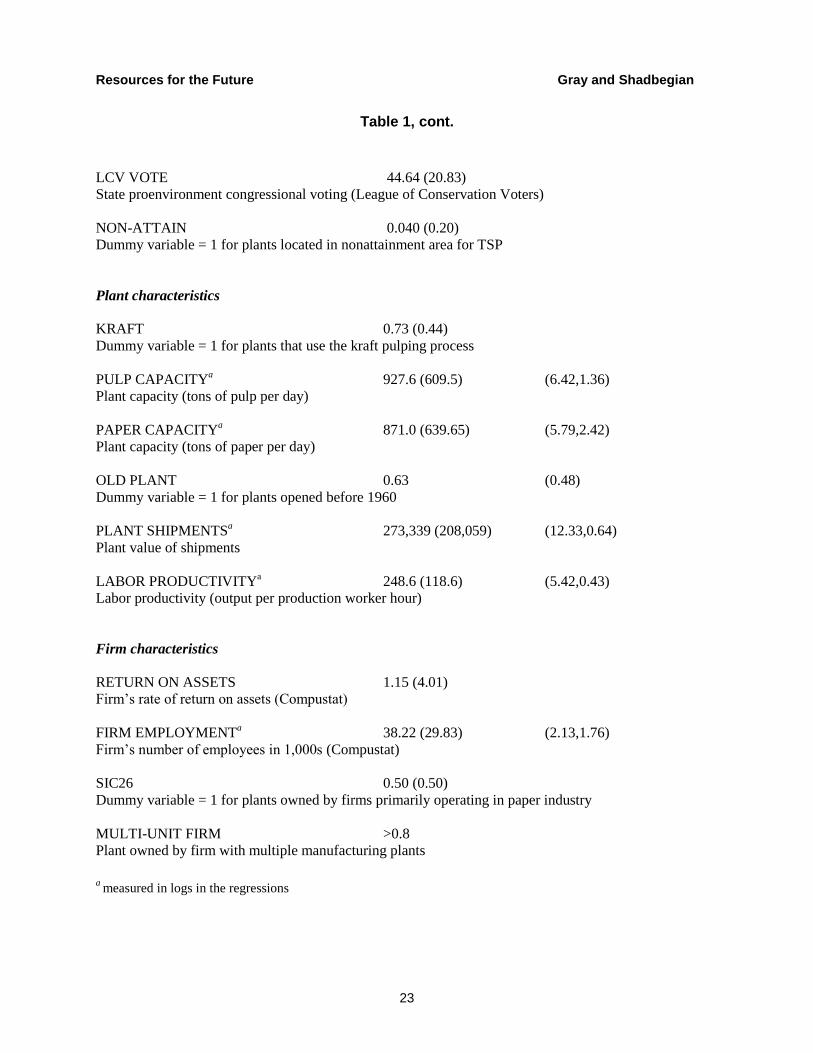
Table 1 presents descriptive statistics for our data. The average plant in our sample
reports nearly a million pounds of toxic releases annually, of which the majority are air toxics.
As noted earlier, most of the dioxin-related substances were not included in the TRI until 2000,
so we focus on releases of chloroform as an indicator of activity that might generate dioxin. We
include separate measures of air and water releases of chloroform. These chloroform releases
Resources for the Future Gray and Shadbegian
13
represent only about 3 percent of total TRI releases. Releases of chloroform are relatively rare,
with only about half of the sample reporting any chloroform releases; this number shrank rapidly
during the years between 1991 and 2009. Most plants in our sample are pre-1960, use kraft
pulping, and belong to multiestablishment firms. Most of the sample was covered by the MACT
air regulations. About half the sample was also covered by the BAT water regulations, and these
show some variability in their start date, on average taking effect slightly before the MACT rules
(in 2000 rather than 2001).
Figure 1 shows the trends over time in average emissions for our six pollutant measures.
Chloroform releases fell dramatically throughout the sample period, with much of the reduction
happening in the 1990s, before the effective date of the Cluster Rule. Air and total toxic releases
increased in the first half of the sample and declined in the second half. PM10 emissions show
some reductions over the sample period, while VOC emissions show some increases.
Our initial ordinary least squares (OLS) analysis of the toxic release data is presented in
columns 1–4 of Table 2. Most of the variables in the model show significant effects and
generally have the expected signs. Our model explains about one-quarter to one-half of the
variation in the emissions measures. Plant characteristics are significant, as expected, with larger
pulping plants and kraft mills having more toxic releases than smaller, nonkraft mills, while the
results for older plants are mixed (less releases overall but more releases for chloroform). Not
surprisingly, plants with more shipments had more releases, while more productive plants had
fewer releases. Firm characteristics show somewhat less consistent effects. More profitable firms
tend to have less releases, though not significant, and multiunit firms have more releases overall.
Firms specializing in the paper industry had less air releases but more chloroform releases.
Larger firms have significantly less chloroform releases (possibly due to large firms being more
sensitive to the bad publicity surrounding dioxin). Our measure of state-level political support for
regulatory stringency, LCV VOTE, is associated with significantly lower releases for all
measures, while being in a nonattainment county is positively associated with chloroform
releases. The results for the conventional air pollutants PM10 and VOCs, shown in columns 5 and
6, are broadly similar for most of the plant characteristics, with greater emissions at larger
pulping plants, plants using kraft pulping, plants with higher shipments and lower productivity,
and plants in less stringent states (as measured by LCV VOTE). A few of the firm characteristics
show differing impacts on PM10 and VOCs, including firm size, multiestablishment firm, and
firms specializing in the paper industry.
Table 2 also includes year dummies, from which we can see whether toxic releases in the
years after the Cluster Rule was implemented appear significantly different (and lower) than
toxic releases in the years before implementation. Note that these year dummies reflect the

Resources for the Future Gray and Shadbegian
14
average experience of all plants in our sample, not just those plants that faced especially strict
MACT or BAT requirements. Air and total releases fell in 2001 relative to the values in 2000 but
remained higher than they were in 1991. Statistical tests for coefficient equality across the year
dummies (at the bottom of Table 2) show essentially no difference within the coefficients in the
later period, but they show significant differences within the earlier period and a significant
difference across all the years in the sample. Chloroform releases show a substantial downward
trend, but the trend begins at the start of the pre-CR period, with a leveling out (at much lower
levels) in the later period. We find significant differences within the pre-CR period and between
the pre- and post-CR periods, but not within the post-CR period. This is consistent with paper
manufacturers taking steps during the 1990s, including the installation of equipment for extended
cooking techniques and oxygen delignification, to reduce their use of chlorine bleaching, even
before the Cluster Rule took effect, with little additional reductions in later years. As noted in
Figure 1, PM10 emissions tended to fall over the period, while VOC emissions increased.
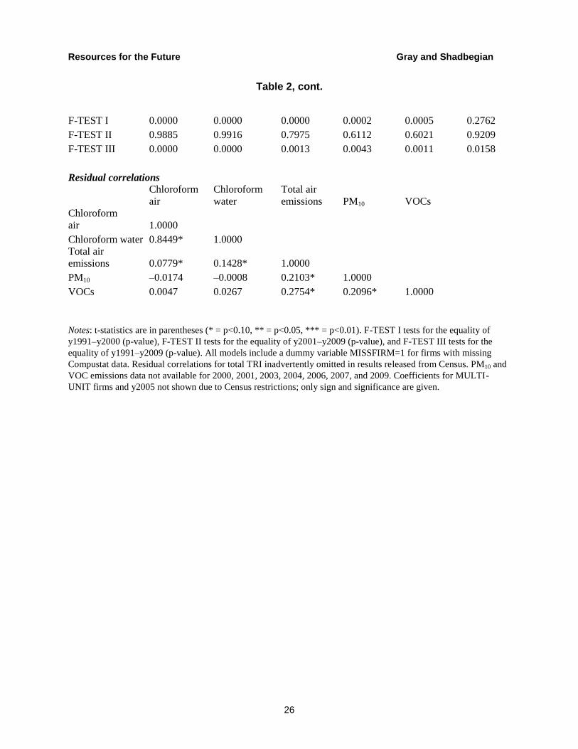
The residual correlations presented at the bottom of Table 2 show a very strong
connection between unexplained air and water releases of chloroform. There are also positive
correlations between unexplained releases of chloroform and other air toxics. Unexplained
emissions of the conventional air pollutants are positively related to each other and to
nonchloroform air toxics but show little relationship to unexplained chloroform releases.
Table 3 presents the results of an analysis that includes plant-specific fixed effects. Most
of the plant-specific characteristics from Table 2 are omitted, as they have no within-plant
variation. Those observations with higher shipments and lower productivity still show greater air
and total releases, and county nonattainment is still associated with greater chloroform releases.
The coefficients on year dummies are also similar to those in Table 2, with the F-tests again
showing significant variation overall and within the pre-CR period, but not within the post-CR
period. However, many of the other coefficients show differences, most notably LCV VOTE,
which shows a surprisingly positive relationship to chloroform releases. Most of the residual
correlations show similar signs to those in Table 2, although the correlations between the air
toxics residual and the conventional air pollutants are not as strong.
Table 4 contains results from OLS models that include measures of the Cluster Rule
requirements that different plants face. We omit a discussion of the coefficients on the control
variables, which are similar to those seen in Table 2. Although we anticipate a general increase
in regulatory stringency around the implementation date, different plants faced different
requirements, and as discussed earlier, there was also some variation in the timing of the BAT
requirements. Some plants faced stricter MACT air requirements, others faced stricter
requirements for both air and water (MACT and BAT), and still others faced neither MACT nor

Resources for the Future Gray and Shadbegian
15
BAT requirements. We include dummy variables indicating whether the plant is covered by the
MACT or BAT rules, along with dummy variables (EFFECTIVE-MACT and EFFECTIVE-
BAT) formed by interacting the MACT and BAT dummies with a time period dummy indicating
when that part of the Cluster Rule requirements took effect for that plant. Since all MACT plants
are also covered by BAT, the MACT coefficients reflect the differences between the MACT-
only plants and the control group of plants unaffected by the CR, while the BAT coefficients
reflect the differences between MACT-only and MACT-plus-BAT plants.
As expected, the MACT coefficients are significantly positive with respect to air and total
toxic releases, reflecting the greater size of those plants relative to the control group, but those
plants do not show substantially larger chloroform releases. On the other hand, the BAT
coefficients show that the BAT plants have similar total and air releases to the MACT-only
plants, while their chloroform releases are much larger. The EFFECTIVE-MACT coefficients
show similar changes over time in air and total toxics in MACT-only and the control plants, with
somewhat greater reductions in chloroform releases. The EFFECTIVE-BAT coefficients are all
significantly negative, and especially large for the chloroform releases, reflecting greater
reductions at BAT plants (compared with MACT-only plants) for all measures of toxic releases.
For both of the conventional air pollutants, the MACT-only plants have higher emissions than
control plants, with somewhat lower emissions at BAT plants (though their emissions are still
higher than those for the control plants). The EFFECTIVE-MACT and EFFECTIVE-BAT
coefficients show little impact on PM10 emissions and some reductions on VOC emissions at
both MACT-only and BAT plants relative to the control plants.
Table 5 shows the impact of including plant-specific fixed effects in the analysis. As with
Table 3, the control variables that do not have any within-plant variation drop out of the analysis.
In this case, that includes the MACT and BAT dummies reflecting the type of CR regulations
faced by the plant. The remaining regulatory variables, EFFECTIVE-MACT and EFFECTIVE-
BAT, show similar results to those found in Table 4. MACT-only plants again show changes in
toxic releases similar to those of the control plants, except for the significant positive coefficient
for total releases. BAT plants again show significantly greater reductions than MACT-only
plants for all toxic releases. For the conventional air pollutants, we see little impacts on PM10
emissions and some reductions (relative to control plants) in VOC emissions, although these
reductions are now larger in BAT plants than in MACT-only plants.
How do the reductions observed for toxic and conventional emissions at MACT and BAT
plants (relative to the control group) compare with the ex ante predictions from EPA? As noted
above, the predictions are that chloroform would be reduced by 99 percent, while air toxics
would fall by 59 percent, VOCs by 49 percent, and PM by 37 percent. The ex post estimated

Resources for the Future Gray and Shadbegian
16
reductions seen in Tables 4 and 5 are fairly similar to these numbers. Summing the EFFECTIVE-
MACT and EFFECTIVE-BAT coefficients and adjusting them for the semilog nature of the
regression,8 we find that BAT plants had reductions in chloroform releases in air by 99 percent
and in water by 96 percent, with essentially the same estimated effects for the OLS and FE
models. The reductions in air toxic releases were not as large as expected, with small and
insignificant effects seen for the MACT-only plants, while BAT plants saw marginally
significant reductions on the order of 17 percent (FE) to 30 percent (OLS). For VOC emissions,
we see sizable reductions in both OLS and FE models, although the models differ on the
estimated impacts. For MACT plants, we see VOC reductions of 52 percent (OLS) and 15
percent (FE); for BAT plants, we see reductions of 58 percent (OLS) and 36 percent (FE). The
changes in PM10 are small and insignificant for both MACT and BAT plants in both OLS and FE
models.
A potential concern with our results is that the MACT and BAT regulations are not
randomly assigned to pulp and paper mills. Rubin (2008) notes that one can approximate a
randomized experiment by selecting a suitably matched control group to eliminate or at least
reduce this bias. We used a version of the propensity score matching (PSM) estimator developed
by Rosenbaum and Rubin (1983) to match each treatment plant (MACT-only or BAT) to a plant
in our control group (with replacement),9 giving us matched pairs of treatment and control plants.
We tested a variety of specifications before achieving the desired “balance” of matching
variables between our treatment and control groups. The final matching model included the
plant’s real output, age, county attainment status, an index of the state’s proenvironmental
congressional voting, and state-year mean wage and employment. Unfortunately, while this
approach provides us with a theoretically more appropriate control group, it also changes our
sample, since a few treatment plants and some control plants from our primary dataset are not
included in the matched sample. Census Bureau rules designed to protect data confidentiality
raise complications for obtaining those results. However, the estimated reductions in toxic and
conventional emissions at MACT and BAT plants (relative to the control group) for the matched
sample are quite similar to the results presented above, in both magnitude and significance. This
provides us with some assurance that our results are not being driven by observable differences
between our treatment and control groups.
8 Percentage impact = exp(coefficient) – 1.
9 To estimate the propensity score and produce our matched control group, we employed the psmatch2 algorithm in
Stata, developed by Leuven and Sianesi (2003).
Resources for the Future Gray and Shadbegian
17
We also compared the actual reductions in emissions with those predicted by our models,
to see whether any plant characteristics were associated with more or less accurate predictions.
We found that prediction accuracy was not related to plant age, but that non-kraft-pulping mills
and smaller-capacity mills tended to have their emissions reductions predicted less accurately
than larger, kraft-pulping mills. The prediction accuracy for reductions in most pollutants were
similar across BAT, MACT-only, and control plants, but the reductions in chloroform emissions
were better predicted for BAT plants, once we eliminated cases of zero emissions (which were
more common for non-BAT plants).
6. Conclusion
In this paper, we have examined the impact of the Cluster Rule on the toxic and
conventional pollution emissions of plants in the pulp and paper industry. This was EPA’s first
integrated, multimedia regulation, combining MACT air regulations and BAT water regulations,
promulgated in 1997 and effective in 2001 (with some variations in effective date across plants,
as described above). We compared EPA’s ex ante estimates of the reductions in different
pollutants to ex post measurements, using a dataset of approximately 150 plants that combines
information from Census, EPA, and industry databases.
In this analysis, our ex post measurements come from regression models implementing a
difference-in-differences strategy, comparing the changes in pollution emissions at regulated
plants around the time the Cluster Rule took effect with changes at plants not covered by the
Cluster Rule, controlling for a variety of plant and firm characteristics. The estimated reductions
in chloroform releases at BAT plants are nearly identical to the ex ante predictions, on the order
of 99 percent. Reductions in air toxics were smaller than expected, especially at the MACT-only
plants. There is some evidence of reductions in VOC emissions, with OLS estimates similar in
magnitude to the ex ante predictions and the FE estimates somewhat smaller; no significant
impact is found on PM10 emissions.
What can we learn from the Cluster Rule about conducting regulatory impact analyses
and retrospective analyses? One justification for the multimedia nature of the Cluster Rule was
that it would reduce compliance costs, relative to using separate air and water regulations. This
seems logical, and research cited here finds compliance costs even lower than EPA’s estimates,
but since the counterfactual of separate air and water regulations is unobserved, retrospective
analyses cannot really judge how much (if anything) was saved by the multimedia approach.
Regulatory flexibility also affects compliance costs, but it can be difficult to identify ex
ante which areas of flexibility will be important. Regulatory impact analyses should carefully
describe the expected compliance methods and potential heterogeneity in methods across plants;

Resources for the Future Gray and Shadbegian
18
retrospective analyses should start by comparing actual compliance methods with those expected
ex ante. This could be especially important in measuring the impact of technological advances in
compliance methods that substantially reduce compliance costs.
Finally, deciding on the appropriate baseline is a necessary step in measuring the benefits
and costs from a regulation. This decision was especially important for the Cluster Rule. Paper
mills faced pressures from state regulators and public opinion to modify their production
processes to reduce dioxin many years before the Cluster Rule took effect. The emissions
reductions and abatement investments that happened before the official baseline were quite
large—possibly even larger than the benefits and costs that happened afterward—and given the
long process of developing the Cluster Rule, EPA had to modify its calculations of benefits and
costs to reflect the changing baseline. It is conceptually as well as practically difficult to
categorize whether the preregulation benefits and costs were done in anticipation of the Cluster
Rule or in response to pressures from state regulation and public opinion. The direct impact of
the Cluster Rule may have been mostly about cleaning up the laggards, but failing to pressure
those laggards might have had adverse consequences for compliance with future regulations.
Future research could extend this analysis in several ways. More detailed data on the
production process used by each plant and the timing of process changes could provide a clearer
picture of how the emissions reductions are achieved. Abatement methods could be connected to
production costs with census microdata and engineering calculations. Heterogeneity in how
different abatement methods affect different types of plants could be examined. The timing of
benefits and costs could also be explored to see how sensitive those calculations are to the choice
of baseline date, likely to be especially important here. Finally, other regulations could be
analyzed to see how broadly applicable our conclusions are.

Resources for the Future Gray and Shadbegian
19
References
Brouhle, Keith, Charles Griffiths, and Ann Wolverton. 2009. Evaluating the Role of EPA Policy
Levers: An Examination of a Voluntary Program and Regulatory Threat in the Metal-
Finishing Industry. Journal of Environmental Economics and Management 57: 166–81.
Bui, L. T. M. 2005. Public Disclosure of Private Information as a Tool for Regulating
Environmental Emissions: Firm-Level Responses by Petroleum Refineries to the Toxics
Release Inventory. Working paper 05-13. Washington, DC: Center for Economic Studies,
US Census Bureau.
Earnhart, D. 2004a. The Effects of Community Characteristics on Polluter Compliance Levels.
Land Economics 80: 408–32.
———. 2004b. Regulatory Factors Shaping Environmental Performance at Publicly-Owned
Treatment Plants. Journal of Environmental Economics and Management 48: 655–81.
EPA (US Environmental Protection Agency). 1998. National Emission Standards for Hazardous
Air Pollutants for Source Category: Pulp and Paper Production; Effluent Limitations
Guidelines, Pretreatment Standards, and New Source Performance Standards: Pulp,
Paper, and Paperboard Category. 63 Fed. Reg. 72, 18504–751.
———. 2010. Guidelines for Preparing Economic Analyses. EPA 240-R-10-0. Washington, DC:
EPA.
———. 2012. Retrospective Cost Study of the Costs of EPA Regulations: An Interim Report of
Five Case Studies. Washington, DC: EPA.
http://yosemite.epa.gov/ee/epa/eed.nsf/Webpages/RetroCost.html/$file/retro-cost-3-30-
12.pdf
Ferguson, K. 1995. Stuck in Environmental Limbo. Pulp & Paper 69 (8): 9.
Glicksman, R., and D. Earnhart. 2007. The Comparative Effectiveness of Government
Interventions on Environmental Performance in the Chemical Industry. Stanford
Environmental Law Journal 26: 317–71.
Gray, W. B., and R. J. Shadbegian. 2003. Plant Vintage, Technology, and Environmental
Regulation. Journal of Environmental Economics and Management 46: 384–402.
———. 2007. The Environmental Performance of Polluting Plants: A Spatial Analysis. Journal
of Regional Science 47: 63–84.

Resources for the Future Gray and Shadbegian
20
———. 2008. Regulatory Regime Changes under Federalism: Do States Matter More?
Presented at First Annual Meeting of the Society for Benefit-Cost Analysis, Washington,
DC, June 25.
Gray, Wayne B., Ronald J. Shadbegian, Chunbei Wang, and Merve Meral. 2014. Do EPA
Regulations Affect Labor Demand? Evidence from the Pulp and Paper Industry. Journal
of Environmental Economics and Management 68: 188–202.
Houck, Oliver A. The Regulation of Toxic Pollutants under the Clean Water Act. Environmental
Law Reporter. 21 ELR 10528. http://elr.info/sites/default/files/articles/21.10528.htm.
Innes, R., and A. Sam. 2008. Voluntary Pollution Reductions and the Enforcement of
Environmental Law: An Empirical Study of the 33/50 Program. Journal of Law and
Economics 51: 271–96.
Jarmin, R. S., and J. Miranda. 2002. The Longitudinal Business Database. Discussion paper
CES-WP-02-17. Washington, DC: Center for Economic Studies, US Census Bureau.
Khanna, M., and Damon, L.A. 1999. EPA’s Voluntary 33/50 Program: Impact on Toxic Releases
and Economic Performance of Firms. Journal of Environmental Economics and
Management 37: 1–25.
Laplante, Benoit, and Paul Rilstone. 1996. Environmental Inspections and Emissions of the Pulp
and Paper Industry in Quebec. Journal of Environmental Economics and Management
31: 19–36.
Leuven, E., and Sianesi, B. 2003. psmatch2: Stata Module to Perform Full Mahalanobis and
Propensity Score Matching, Common Support Graphing, and Covariate Imbalance
Testing. http://ideas.repec.org/c/boc/bocode/s432001.html.
Lockwood-Post Pulp and Paper Directory. Various dates. San Francisco: Miller-Freeman
Publishing Company.
Magat, W. A., and W. K. Viscusi. 1990. Effectiveness of the EPA’s Regulatory Enforcement:
The Case of Industrial Effluent Standards. Journal of Law and Economics 33: 331–60.
Maynard, L. J., and J. S. Shortle. 2001. Determinants of cleaner technology investments in the
U.S. Bleached Kraft Pulp Industry. Land Economics 71 (4): 561–76.
Morgan, C., C. A. Pasurka, and R. J. Shadbegian. 2014. Ex Ante and Ex Post Cost Estimates of
the Cluster Rule and MACT II Rule. Journal of Benefit-Cost Analysis 5: 195–224.
Popp, David, and Tamara Hafner. 2008. Policy versus Consumer Pressure: Innovation and
Diffusion of Alternative Bleaching Technologies in the Pulp Industry. In Environmental

Resources for the Future Gray and Shadbegian
21
Policy, Technological Innovation and Patents, OECD Studies on Environmental
Innovation, 107–38. Paris: OECD Publications.
Rosenbaum, P., and D. Rubin. 1983. The Central Role of the Propensity Score in Observational
Studies for Causal Effects. Biometrika 70: 41–55.
Rubin, D. 2008. For Objective Causal Inference, Design Trumps Analysis. Annals of Applied
Statistics 2: 808–40.
Shadbegian, R. J., and W. B. Gray. 2003. What Determines the Environmental Performance of
Paper Mills? The Roles of Abatement Spending, Regulation, and Efficiency. Topics in
Economic Analysis & Policy 3. http://www.bepress.com/bejeap/topics/vol3/iss1/art15.
Shadbegian, R. J., and W. B. Gray. 2006. Assessing Multi-dimensional Performance:
Environmental and Economic Outcomes. Journal of Productivity Analysis 26: 213–34.
Shimshack, Jay P., and Michael B. Ward. 2005. Regulator Reputation, Enforcement, and
Environmental Compliance. Journal of Environmental Economics and Management 50:
519–40.
———. 2008. Enforcement and Over-compliance. Journal of Environmental Economics and
Management 55: 90–105.
Snyder, Lori D., Nolan H. Miller, and Robert N. Stavins. 2003. The Effects of Environmental
Regulation on Technology Diffusion: The Case of Chlorine Manufacturing. American
Economic Review 93 (2): 431–35.

Resources for the Future Gray and Shadbegian
22
Tables and Figures
Table 1. Descriptive Statistics (N = 2251 unless otherwise noted)
Variable Mean (std. dev.) {log m,sd}
Dependent Variables
AIR CHLOROFORM EMISSIONSa 30687.2 (83073.41) {3.12,5.02}
Total chloroform air releases (in pounds)
WATER CHLOROFORM EMISSIONSa 981.5 (6083.27) {1.72,3.12}
Total chloroform water releases (in pounds)
TOTAL AIR EMISSIONSa 785065.0 (834442.8) {2.69,4.75}
Total toxic air releases (in pounds)
TOTAL TRI EMISSIONSa 969205.0 (998839.4) {11.51,3.75}
Total toxic releases (in pounds)
PM10 (N = 1122)a 576.6 (647.9) {5.11,1.86}
Tons of particulate emissions per year
VOCs (N = 1122)a 631.6 (766.8) {5.59,1.72}
Tons of volatile organic compound emissions per year
Explanatory Variables
Regulatory-related characteristics
MACT 0.79 (0.41)
Dummy variable = 1 for plants that must install maximum available control technology to abate toxic air
emissions
EFFECTIVE-MACT 0.34 (0.47)
Dummy variable = 1 for MACT plants after 2000
BAT 0.53 (0.50)
Dummy variable = 1 for plants that must install best available technology to abate toxic water releases
EFFECTIVE-BAT 0.25 (0.43)
Dummy variable = 1 for BAT plants with timing based on date of plant’s water permit
Resources for the Future Gray and Shadbegian
23
Table 1, cont.
LCV VOTE 44.64 (20.83)
State proenvironment congressional voting (League of Conservation Voters)
NON-ATTAIN 0.040 (0.20)
Dummy variable = 1 for plants located in nonattainment area for TSP
Plant characteristics
KRAFT 0.73 (0.44)
Dummy variable = 1 for plants that use the kraft pulping process
PULP CAPACITYa 927.6 (609.5) (6.42,1.36)
Plant capacity (tons of pulp per day)
PAPER CAPACITYa 871.0 (639.65) (5.79,2.42)
Plant capacity (tons of paper per day)
OLD PLANT 0.63 (0.48)
Dummy variable = 1 for plants opened before 1960
PLANT SHIPMENTSa 273,339 (208,059) (12.33,0.64)
Plant value of shipments
LABOR PRODUCTIVITYa 248.6 (118.6) (5.42,0.43)
Labor productivity (output per production worker hour)
Firm characteristics
RETURN ON ASSETS 1.15 (4.01)
Firm’s rate of return on assets (Compustat)
FIRM EMPLOYMENTa
38.22 (29.83) (2.13,1.76)
Firm’s number of employees in 1,000s (Compustat)
SIC26 0.50 (0.50)
Dummy variable = 1 for plants owned by firms primarily operating in paper industry
MULTI-UNIT FIRM >0.8
Plant owned by firm with multiple manufacturing plants
a measured in logs in the regressions

Resources for the Future Gray and Shadbegian
24
Table 2. Basic OLS Models
Dep. var.
Chloroform
air
Chloroform
water
Total air
emissions
Total TRI
emissions PM10 VOCs
Plant characteristics
KRAFT 0.445** 0.400*** 2.524*** 1.913*** 0.978*** 0.215*
(0.222) (0.142) (0.131) (0.114) (0.092) (0.113)
PULP 0.450*** 0.276*** 0.682*** 0.682*** 0.311*** 0.272***
CAPACITY (0.077) (0.049) (0.045) (0.040) (0.032) (0.040)
PAPER –0.560*** –0.298*** –0.010 –0.061*** –0.088*** –0.023
CAPACITY (0.041) (0.026) (0.024) (0.021) (0.017) (0.021)
OLD PLANT 0.917*** 0.457*** –0.399*** –0.314*** –0.362*** –0.017
(0.206) (0.131) (0.122) (0.106) (0.088) (0.108)
PLANT 1.541*** 0.834*** 0.764*** 0.766*** 0.853*** 0.838***
SHIPMENTS (0.164) (0.104) (0.097) (0.084) (0.068) (0.084)
LABOR –1.255*** –0.891*** –0.695*** –0.628*** –0.742*** –0.556***
PRODUCTIVITY (0.287) (0.183) (0.170) (0.148) (0.128) (0.157)
Firm characteristics
RETURN ON –2.648 0.002 –1.084 –2.065 –1.089 –1.378
ASSETS (2.456) (1.564) (1.452) (1.263) (0.870) (1.066)
FIRM –0.476*** –0.184*** 0.038 0.074 0.069 –0.157***
EMPLOYMENT (0.102) (0.065) (0.060) (0.052) (0.044) (0.054)
SIC26 0.219 –0.234 –0.315** –0.152 –0.284*** 0.050
(0.256) (0.163) (0.151) (0.131) (0.104) (0.127)
MULTI-UNIT – – +*** +*** –*** +
FIRM
Plant regulation
LCV VOTE –0.013*** –0.008** –0.015*** –0.014*** –0.014*** –0.016***
(0.005) (0.003) (0.003) (0.003) (0.002) (0.003)
NON-ATTAIN 1.091** 0.887*** 0.109 0.019 0.297* 0.543**
(0.452) (0.288) (0.267) (0.233) (0.178) (0.218)

Resources for the Future Gray and Shadbegian
25
Table 2, cont.
Pre–Cluster Rule
y1992 –0.280 –0.298 0.159 0.052 –0.087 0.060
(0.516) (0.329) (0.305) (0.265) (0.172) (0.211)
y1993 –0.242 –0.214 0.165 0.065 0.212 0.339
(0.517) (0.329) (0.306) (0.266) (0.172) (0.211)
y1994 –0.879* –0.648* 0.966*** 0.761*** 0.237 0.448**
(0.519) (0.331) (0.307) (0.267) (0.172) (0.211)
y1995 –1.627*** –1.269*** 0.854*** 0.554** –0.051 0.291
(0.532) (0.339) (0.314) (0.273) (0.177) (0.217)
y1996 –2.082*** –1.605*** 0.901*** 0.656** –0.335** 0.418**
(0.520) (0.331) (0.307) (0.267) (0.171) (0.209)
y1997 –2.664*** –1.859*** 1.002*** 0.750*** –0.335* 0.415**
(0.519) (0.331) (0.307) (0.267) (0.171) (0.209)
y1998 –3.003*** –2.110*** 1.180*** 0.943*** –0.311* 0.420*
(0.535) (0.341) (0.316) (0.275) (0.178) (0.218)
y1999 –3.323*** –2.215*** 1.174*** 0.851*** –0.342* 0.445**
(0.543) (0.346) (0.321) (0.279) (0.181) (0.222)
y2000 –4.385*** –2.850*** 1.156*** 0.879*** . .
(0.539) (0.343) (0.319) (0.277)
Post–Cluster Rule
Y2001 –5.358*** –3.340*** 0.609* 0.358 . .
(0.538) (0.342) (0.318) (0.276)
y2002 –5.570*** –3.515*** 0.812** 0.637** –0.325* 0.949***
(0.547) (0.348) (0.323) (0.281) (0.189) (0.231)
y2003 –5.736*** –3.650*** 0.900*** 0.651** . .
(0.563) (0.358) (0.333) (0.289)
y2004 –5.816*** –3.663*** 1.115*** 0.877*** . .
(0.564) (0.359) (0.333) (0.290)
y2005 –5.913*** –3.655*** 1.048*** 0.826*** + +
(0.571) (0.364) (0.337) (0.294)
y2006 –5.762*** –3.585*** 1.053*** 0.858*** . .
(0.576) (0.367) (0.341) (0.296)
y2007 –5.764*** –3.580*** 1.011*** 0.802*** . .
(0.584) (0.372) (0.345) (0.300)
y2008 –5.796*** –3.532*** 1.172*** 0.927*** –0.455** 0.875***
(0.590) (0.376) (0.349) (0.304) (0.209) (0.256)
y2009 –5.488*** –3.438*** 0.931*** 0.695** . .
(0.588) (0.374) (0.347) (0.302)
N 2251 2251 2251 2251 1122 1122
R2 0.335 0.299 0.425 0.443 .401 .242
Resources for the Future Gray and Shadbegian
26
Table 2, cont.
F-TEST I 0.0000 0.0000 0.0000 0.0002 0.0005 0.2762
F-TEST II 0.9885 0.9916 0.7975 0.6112 0.6021 0.9209
F-TEST III 0.0000 0.0000 0.0013 0.0043 0.0011 0.0158
Residual correlations
Chloroform
air
Chloroform
water
Total air
emissions PM10 VOCs
Chloroform
air 1.0000
Chloroform water 0.8449* 1.0000
Total air
emissions 0.0779* 0.1428* 1.0000
PM10 –0.0174 –0.0008 0.2103* 1.0000
VOCs 0.0047 0.0267 0.2754* 0.2096* 1.0000
Notes: t-statistics are in parentheses (* = p<0.10, ** = p<0.05, *** = p<0.01). F-TEST I tests for the equality of
y1991–y2000 (p-value), F-TEST II tests for the equality of y2001–y2009 (p-value), and F-TEST III tests for the
equality of y1991–y2009 (p-value). All models include a dummy variable MISSFIRM=1 for firms with missing
Compustat data. Residual correlations for total TRI inadvertently omitted in results released from Census. PM10 and
VOC emissions data not available for 2000, 2001, 2003, 2004, 2006, 2007, and 2009. Coefficients for MULTI-
UNIT firms and y2005 not shown due to Census restrictions; only sign and significance are given.

Resources for the Future Gray and Shadbegian
27
Table 3. Basic FE Models
Dep. var.
Chloroform
air
Chloroform
water
Total air
emissions
Total TRI
emissions PM10 VOCs
Plant characteristics
PLANT 0.246 0.146 0.582*** 0.258** 0.680*** 0.489***
SHIPMENTS (0.271) (0.171) (0.140) (0.123) (0.094) (0.125)
LABOR 0.069 0.075 –0.474** –0.321* –0.527*** –0.971***
PRODUCTIVITY (0.408) (0.257) (0.211) (0.185) (0.164) (0.217)
Firm characteristics
RETURN ON 1.246 2.017 2.138** 0.264 –1.418** –0.056
ASSETS (2.050) (1.292) (1.061) (0.928) (0.594) (0.785)
FIRM –0.146 –0.106 0.139** 0.053 –0.009 –0.222***
EMPLOYMENT (0.129) (0.082) (0.067) (0.059) (0.053) (0.070)
SIC26 1.791*** 1.019*** 0.357 0.223 –0.288* 0.222
(0.498) (0.314) (0.258) (0.225) (0.161) (0.214)
MULTI-UNIT –*** –*** – – –*** +
FIRM
Plant regulation
LCV VOTE 0.019** 0.013** –0.004 –0.005 –0.005 0.012***
(0.009) (0.005) (0.004) (0.004) (0.003) (0.004)
NON-ATTAIN 1.387** 1.188*** –0.131 –0.193 0.454** 0.246
(0.573) (0.361) (0.297) (0.259) (0.181) (0.239)
Pre–Cluster Rule
y1992 0.058 –0.074 0.167 0.056 0.008 0.207
(0.406) (0.256) (0.210) (0.184) (0.105) (0.139)
y1993 –0.522 –0.396 0.000 –0.075 0.154 0.022
(0.406) (0.256) (0.210) (0.184) (0.105) (0.139)
y1994 –1.157*** –0.826*** 0.654*** 0.460** 0.203* 0.217
(0.405) (0.255) (0.210) (0.183) (0.104) (0.137)
y1995 –1.554*** –1.230*** 0.614*** 0.352* 0.106 0.360**
(0.422) (0.266) (0.219) (0.191) (0.109) (0.144)
y1996 –1.951*** –1.559*** 0.777*** 0.530*** –0.146 0.457***
(0.410) (0.258) (0.212) (0.186) (0.104) (0.138)
y1997 –2.478*** –1.753*** 0.903*** 0.700*** –0.205** 0.458***
(0.408) (0.257) (0.211) (0.185) (0.104) (0.138)
y1998 –2.943*** –2.120*** 0.966*** 0.795*** –0.197* 0.581***
(0.431) (0.272) (0.223) (0.195) (0.115) (0.153)
y1999 –3.293*** –2.240*** 1.051*** 0.806*** –0.179 0.649***
(0.443) (0.279) (0.229) (0.201) (0.120) (0.159)
y2000 –4.432*** –2.921*** 1.000*** 0.725*** . .
(0.441) (0.278) (0.228) (0.200)

Resources for the Future Gray and Shadbegian
28
Table 3, cont.
Post–Cluster Rule
Y2001 –5.536*** –3.450*** 0.514** 0.352* . .
(0.443) (0.279) (0.229) (0.200)
y2002 –5.946*** –3.736*** 0.438* 0.266 –0.216 1.102***
(0.459) (0.289) (0.238) (0.208) (0.135) (0.178)
y2003 –6.106*** –3.849*** 0.544** 0.354* . .
(0.467) (0.294) (0.242) (0.211)
y2004 –6.197*** –3.863*** 0.615** 0.448** . .
(0.472) (0.297) (0.244) (0.214)
y2005 –6.225*** –3.814*** 0.598** 0.424* – +*
(0.480) (0.303) (0.249) (0.218)
y2006 –6.167*** –3.819*** 0.544** 0.389* . .
(0.489) (0.308) (0.253) (0.222)
y2007 –6.358*** –3.937*** 0.536** 0.384* . .
(0.493) (0.311) (0.255) (0.223)
y2008 –6.355*** –3.891*** 0.779*** 0.546** –0.538*** 0.812***
(0.497) (0.313) (0.257) (0.225) (0.151) (0.199)
y2009 –6.318*** –3.925*** 0.457* 0.216 . .
(0.491) (0.309) (0.254) (0.222)
N 2251 2251 2251 2251 1122 1122
R2 0.615 0.603 0.745 0.750 0.795 0.698
F-TEST I 0.0000 0.0000 0.0000 0.0000 0.0001 0.0003
F-TEST II 0.6659 0.7664 0.9220 0.8676 0.0219 0.1414
F-TEST III 0.0000 0.0000 0.0000 0.0000 0.0003 0.0000
Residual correlations
Chloroform
air
Chloroform
water
Total air
emissions PM10 VOCs
Chloroform
air 1.0000
Chloroform water 0.8423* 1.0000
Total air
emissions 0.0263 0.0565* 1.0000
PM10 0.0416 0.0524 –0.0012 1.0000
VOCs 0.0276 0.0550 0.0724* 0.2649* 1.0000
Note: See Table 2.

Resources for the Future Gray and Shadbegian
29
Table 4. Extended OLS Models
Dep. var.
Chloroform
air
Chloroform
water
Total air
emissions
Total TRI
emissions PM10 VOCs
MACT –0.260 0.050 2.498*** 1.901*** 0.794*** 1.223***
(0.321) (0.210) (0.200) (0.175) (0.131) (0.159)
EFFECTIVE- –0.648 –0.502* –0.006 0.253 0.009 –0.739**
MACT (0.432) (0.282) (0.269) (0.235) (0.277) (0.336)
BAT 5.381*** 3.007*** 0.085 0.226 –0.272*** –0.224*
(0.259) (0.170) (0.162) (0.141) (0.103) (0.125)
EFFECTIVE- –5.085*** –2.780*** –0.345* –0.392** –0.021 –0.138
BAT (0.323) (0.211) (0.201) (0.176) (0.187) (0.226)
Plant characteristics
KRAFT 0.261 0.258* 1.840*** 1.345*** 0.836*** 0.028
(0.208) (0.136) (0.129) (0.113) (0.094) (0.114)
PULP 0.427*** 0.252*** 0.493*** 0.531*** 0.243*** 0.168***
CAPACITY (0.071) (0.047) (0.044) (0.039) (0.034) (0.041)
PAPER –0.462*** –0.238*** 0.062*** 0.001 –0.072*** 0.002
CAPACITY (0.037) (0.024) (0.023) (0.020) (0.017) (0.021)
OLD PLANT 1.062*** 0.545*** –0.291** –0.217** –0.332*** 0.040
(0.183) (0.120) (0.114) (0.100) (0.087) (0.106)
PLANT 0.538*** 0.249** 0.532*** 0.541*** 0.897*** 0.845***
SHIPMENTS (0.160) (0.105) (0.100) (0.087) (0.075) (0.091)
LABOR –0.012 –0.165 –0.372** –0.311** –0.773*** –0.539***
PRODUCTIVITY (0.272) (0.178) (0.169) (0.148) (0.132) (0.160)
Firm characteristics
RETURN ON –1.072 0.973 –0.860 –1.829 –1.367 –1.805*
ASSETS (2.197) (1.436) (1.369) (1.197) (0.865) (1.048)
FIRM –0.518*** –0.206*** 0.055 0.087* 0.070 –0.161***
EMPLOYMENT (0.090) (0.059) (0.056) (0.049) (0.043) (0.052)
SIC26 0.580** –0.011 –0.010 0.117 –0.265** 0.086
(0.230) (0.151) (0.143) (0.126) (0.103) (0.125)
MULTI-UNIT + + +*** +*** –*** +
FIRM
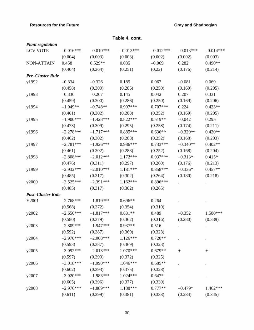
Resources for the Future Gray and Shadbegian
30
Table 4, cont.
Plant regulation
LCV VOTE –0.016*** –0.010*** –0.013*** –0.012*** –0.013*** –0.014***
(0.004) (0.003) (0.003) (0.002) (0.002) (0.003)
NON-ATTAIN 0.458 0.529** 0.035 –0.069 0.282 0.490**
(0.404) (0.264) (0.251) (0.22) (0.176) (0.214)
Pre–Cluster Rule
y1992 –0.334 –0.326 0.185 0.067 –0.081 0.069
(0.458) (0.300) (0.286) (0.250) (0.169) (0.205)
y1993 –0.336 –0.267 0.145 0.042 0.207 0.331
(0.459) (0.300) (0.286) (0.250) (0.169) (0.206)
y1994 –1.049** –0.748** 0.907*** 0.707*** 0.224 0.423**
(0.461) (0.302) (0.288) (0.252) (0.169) (0.205)
y1995 –1.900*** –1.428*** 0.822*** 0.519** –0.042 0.295
(0.473) (0.309) (0.295) (0.258) (0.174) (0.211)
y1996 –2.278*** –1.717*** 0.885*** 0.636** –0.329** 0.420**
(0.462) (0.302) (0.288) (0.252) (0.168) (0.203)
y1997 –2.781*** –1.926*** 0.986*** 0.733*** –0.340** 0.402**
(0.461) (0.302) (0.288) (0.252) (0.168) (0.204)
y1998 –2.808*** –2.012*** 1.172*** 0.937*** –0.313* 0.415*
(0.476) (0.311) (0.297) (0.260) (0.176) (0.213)
y1999 –2.932*** –2.010*** 1.181*** 0.858*** –0.336* 0.457**
(0.485) (0.317) (0.302) (0.264) (0.180) (0.218)
y2000 –3.525*** –2.391*** 1.162*** 0.896*** . .
(0.485) (0.317) (0.302) (0.265)
Post–Cluster Rule
Y2001 –2.768*** –1.819*** 0.696** 0.264 . .
(0.568) (0.372) (0.354) (0.310)
y2002 –2.650*** –1.817*** 0.831** 0.489 –0.352 1.580***
(0.580) (0.379) (0.362) (0.316) (0.280) (0.339)
y2003 –2.809*** –1.947*** 0.937** 0.516 . .
(0.592) (0.387) (0.369) (0.323)
y2004 –2.970*** –2.008*** 1.126*** 0.720** . .
(0.593) (0.387) (0.369) (0.323)
y2005 –3.092*** –2.013*** 1.070*** 0.679** + +
(0.597) (0.390) (0.372) (0.325)
y2006 –3.018*** –1.990*** 1.046*** 0.685** . .
(0.602) (0.393) (0.375) (0.328)
y2007 –3.020*** –1.983*** 1.024*** 0.647* . .
(0.605) (0.396) (0.377) (0.330)
y2008 –2.976*** –1.889*** 1.188*** 0.777** –0.479* 1.462***
(0.611) (0.399) (0.381) (0.333) (0.284) (0.345)
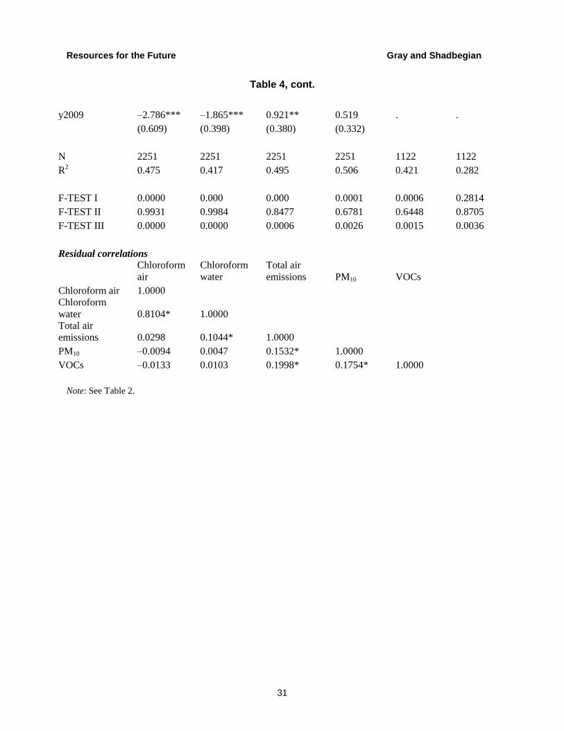
Resources for the Future Gray and Shadbegian
31
Table 4, cont.
y2009 –2.786*** –1.865*** 0.921** 0.519 . .
(0.609) (0.398) (0.380) (0.332)
N 2251 2251 2251 2251 1122 1122
R2 0.475 0.417 0.495 0.506 0.421 0.282
F-TEST I 0.0000 0.000 0.000 0.0001 0.0006 0.2814
F-TEST II 0.9931 0.9984 0.8477 0.6781 0.6448 0.8705
F-TEST III 0.0000 0.0000 0.0006 0.0026 0.0015 0.0036
Residual correlations
Chloroform
air
Chloroform
water
Total air
emissions PM10 VOCs
Chloroform air 1.0000
Chloroform
water 0.8104* 1.0000
Total air
emissions 0.0298 0.1044* 1.0000
PM10 –0.0094 0.0047 0.1532* 1.0000
VOCs –0.0133 0.0103 0.1998* 0.1754* 1.0000
Note: See Table 2.

Resources for the Future Gray and Shadbegian
32
Table 5. Extended FE Models
Dep. var.
Chloroform
air
Chloroform
water
Total air
emissions
Total
TRI
emissions PM10 VOCs
EFFECTIVE- –0.151 –0.128 0.139 0.363** 0.115 –0.163
MACT (0.341) (0.222) (0.200) (0.175) (0.182) (0.241)
EFFECTIVE- –5.499*** –3.031*** –0.330** –0.395*** –0.108 –0.283*
BAT (0.253) (0.165) (0.149) (0.130) (0.119) (0.157)
Plant characteristics
PLANT –0.008 0.006 0.567*** 0.240* 0.672*** 0.469***
SHIPMENTS (0.239) (0.156) (0.141) (0.123) (0.095) (0.125)
LABOR –0.034 0.016 –0.473** –0.312* –0.516*** –0.920***
PRODUCTIVITY (0.360) (0.234) (0.211) (0.185) (0.165) (0.217)
Firm characteristics
RETURN ON –0.565 1.025 2.009* 0.084 –1.486** –0.278
ASSETS (1.811) (1.178) (1.062) (0.928) (0.599) (0.791)
FIRM –0.189* –0.129* 0.136** 0.049 –0.011 –0.231***
EMPLOYMENT (0.114) (0.074) (0.067) (0.059) (0.053) (0.070)
SIC26 0.990** 0.573** 0.323 0.202 –0.285* 0.195
(0.440) (0.287) (0.258) (0.226) (0.162) (0.214)
MULTI-UNIT –* – – – –*** +
FIRM
Plant regulation
LCV VOTE 0.026*** 0.017*** –0.004 –0.004 –0.004 0.012***
(0.008) (0.005) (0.004) (0.004) (0.003) (0.004)
NON-ATTAIN 0.725 0.822** –0.167 –0.231 0.451** 0.242
(0.506) (0.329) (0.297) (0.259) (0.181) (0.239)
Pre–Cluster Rule
y1992 –0.005 –0.109 0.163 0.052 0.008 0.206
(0.358) (0.233) (0.210) (0.183) (0.105) (0.138)
y1993 –0.703** –0.496** –0.011 –0.091 0.152 0.021
(0.358) (0.233) (0.210) (0.184) (0.105) (0.139)
y1994 –1.265*** –0.886*** 0.649*** 0.455** 0.202* 0.215
(0.357) (0.232) (0.210) (0.183) (0.104) (0.137)
y1995 –1.527*** –1.216*** 0.617*** 0.359* 0.109 0.365**
(0.372) (0.242) (0.218) (0.191) (0.109) (0.144)
y1996 –2.004*** –1.588*** 0.775*** 0.530*** –0.146 0.456***
(0.361) (0.235) (0.212) (0.185) (0.105) (0.138)
y1997 –2.559*** –1.798*** 0.899*** 0.695*** –0.205** 0.452***
(0.359) (0.234) (0.211) (0.184) (0.104) (0.137)
y1998 –2.444*** –1.845*** 0.996*** 0.831*** –0.190 0.589***
(0.381) (0.248) (0.223) (0.195) (0.116) (0.153)

Resources for the Future Gray and Shadbegian
33
Table 5, cont.
y1999 –2.537*** –1.824*** 1.096*** 0.858*** –0.166 0.669***
(0.392) (0.255) (0.230) (0.201) (0.121) (0.160)
y2000 –3.074*** –2.172*** 1.081*** 0.820*** . .
(0.394) (0.256) (0.231) (0.202)
Post–Cluster Rule
Y2001 –2.807*** –1.910*** 0.560** 0.250 . .
(0.460) (0.299) (0.270) (0.236)
y2002 –2.767*** –1.946*** 0.507* 0.187 –0.257 1.372***
(0.477) (0.310) (0.280) (0.245) (0.191) (0.252)
y2003 –2.978*** –2.089*** 0.610** 0.271 . .
(0.482) (0.314) (0.283) (0.247)
y2004 –3.047*** –2.091*** 0.682** 0.369 . .
(0.485) (0.316) (0.285) (0.249)
y2005 –3.116*** –2.064*** 0.664** 0.344 – +**
(0.491) (0.319) (0.288) (0.252)
y2006 –3.077*** –2.080*** 0.609** 0.308 . .
(0.498) (0.324) (0.292) (0.255)
y2007 –3.311*** –2.221*** 0.600** 0.302 . .
(0.500) (0.325) (0.293) (0.256)
y2008 –3.416*** –2.235*** 0.834*** 0.452* –0.579*** 1.056***
(0.504) (0.328) (0.296) (0.259) (0.197) (0.261)
y2009 –3.362*** –2.260*** 0.515* 0.125 . .
(0.499) (0.324) (0.293) (0.256)
N 2251 2251 2251 2251 1122 1122
R2 0.701 0.671 0.745 0.751 0.795 0.699
F-TEST I 0.0000 0.0000 0.0000 0.0000 0.0002 0.0002
F-TEST II 0.7194 0.8904 0.9234 0.8647 0.0215 0.1164
F-TEST III 0.0000 0.0000 0.0000 0.0000 0.0003 0.0000

Resources for the Future Gray and Shadbegian
34
Table 5, cont.
Residual correlations
Chloroform
air
Chloroform
water
Total air
emissions PM10 VOCs
Chloroform air 1.0000
Chloroform
water 0.8057* 1.0000
Total air
emissions 0.0049 0.0410 1.0000
PM10 0.0395 0.0510 –0.0024 1.0000
VOCs 0.0064 0.0389 0.0667* 0.2645* 1.0000
Note: See Table 2.
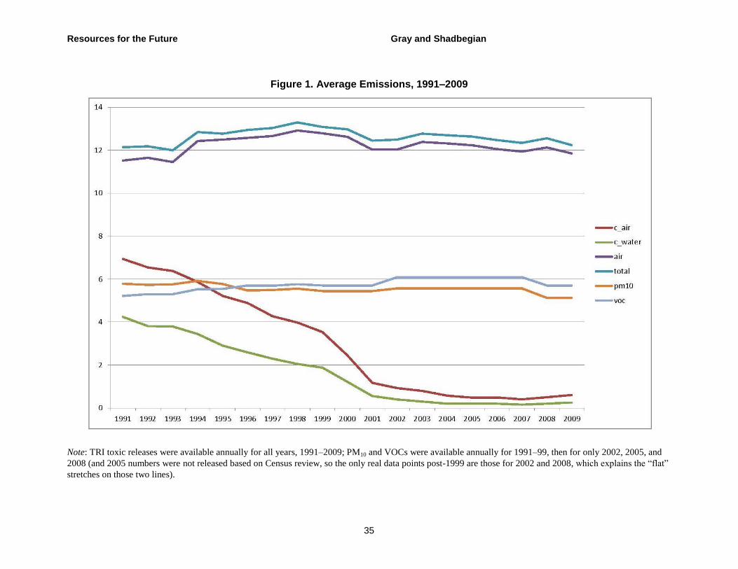
Resources for the Future Gray and Shadbegian
35
Figure 1. Average Emissions, 1991–2009
Note: TRI toxic releases were available annually for all years, 1991–2009; PM10 and VOCs were available annually for 1991–99, then for only 2002, 2005, and
2008 (and 2005 numbers were not released based on Census review, so the only real data points post-1999 are those for 2002 and 2008, which explains the “flat”
stretches on those two lines).