august 2009 rff dp 09-24 discussion paper

1616 P St. NW Washington, DC 20036 202-328-5000 www.rff.org

August 2009 RFF DP 09-24

Conflicting Goals: Energy Security versus GHG Reductions under the EISA Cellulosic Ethanol Mandate

Ar thur F raas and Rober t J ohansson

DIS

CU

SSIO

N P

APE

R

© 2009 Resources for the Future. All rights reserved. No portion of this paper may be reproduced without permission of the authors.

Discussion papers are research materials circulated by their authors for purposes of information and discussion. They have not necessarily undergone formal peer review.

Conflicting Goals: Energy Security vs. GHG Reductions under the EISA Cellulosic Ethanol Mandate

Arthur Fraas and Robert Johansson

Abstract Increasing energy security and lowering greenhouse gas (GHG) emissions have been prominent

goals in recent energy and environmental policies. While these goals are often complementary, there may also be cases where they conflict. A case in point is the Energy Independence and Security Act of 2007 (EISA). The goals of EISA are to increase the United States' energy independence and security as well as to increase the production of clean renewable fuels. Title II of EISA establishes mandates for increasing the use of low carbon fuels to replace gasoline. While the Title II mandates will meet the energy security goal of EISA, the mandate for the use of at least 16 billion gallons of cellulosic ethanol by 2022 may conflict with efforts to reduce substantially the nation's GHG emissions over the next 20 years. The nation's production capacity for biomass is likely to be limited and the use of biomass to replace coal in generating electricity yields 2 to 3 times the GHG reduction associated with using cellulosic ethanol to displace gasoline. Thus, there is a trade-off between the energy security gains of the biofuels mandate under EISA and the more effective (in terms of GHG emission reductions) use of biomass in the electric utility sector. One means of evaluating this trade-off is to examine the factors that affect the cost-effectiveness of diverting biomass from electricity production to cellulosic ethanol production. This paper identifies some of the key factors that affect the cost-effectiveness of the energy security and climate change goals of EISA. The cost-effectiveness of EISA will depend on (1) constraints on biomass production, that is, the extent to which the EISA mandate may crowd out the use of biomass to generate electricity; (2) the world oil price (and the cost of production of cellulosic ethanol); and (3) the social cost of carbon.

Key Words: energy security, cost-effective policy, cellulosic ethanol

JEL Classification Numbers: Q42, Q48, Q52

Contents

Introduction ............................................................................................................................. 1

Background ............................................................................................................................. 3

Framework and Assumptions .............................................................................................. 11

Results .................................................................................................................................... 17

Conclusion ............................................................................................................................. 24

Appendix A. Calculation of GHG Reductions ................................................................... 26

Appendix B. Ethanol GHG Reductions .............................................................................. 28

Appendix C. Example Calculations .................................................................................... 29

Resources for the Future Fraas and Johansson

1

Conflicting Goals: Energy Security vs. GHG Reductions under the EISA Cellulosic Ethanol Mandate

Arthur Fraas and Robert Johansson∗

Introduction

The United States imports more than 60 percent of its petroleum supply. In 2006, crude oil plus petroleum product imports cost the United States roughly $220 billion. Many argue that burning ethanol in U.S. automobiles is a cost-effective way of lowering U.S. dependence on petroleum imports. As discussed below, the Energy Security and Independence Act of 2007 (EISA) seeks to do just that—promote the use of biomass to displace imported petroleum in meeting the U.S. demand for liquid transportation fuels. By 2022, EISA would require the use of 36 billion gallons of biofuel in the United States, up from the current level of roughly 10.5 billion gallons. To meet this requirement, the United States is expected to produce increasing amounts of corn ethanol, biodiesel, cellulosic ethanol, and other advanced biofuels.

In addition, burning gasoline or diesel in an engine produces a variety of pollutants including carbon dioxide, a greenhouse gas (GHG). Each gallon of gasoline burned releases over 20 pounds of carbon dioxide--in aggregate the transportation sector emits about 17 percent of the total U.S. emissions of GHGs. Cellulosic ethanol is a "renewable" fuel derived from biomass and its use is expected to lower GHG emissions relative to gasoline use by as much as 50 percent to 90 percent per gallon of gasoline displaced.

However, turning on our computers, drying our clothes, and cooling our houses require electricity as an energy source. Most of the electricity used in the United States is generated by using fuel (or other energy sources) produced within the country, so there is no energy security issue associated with electricity production and use. However, roughly half of the electricity used in day-to-day activities comes from coal found in states like Wyoming and West Virginia. That coal is mined, transported to electric utilities, pulverized to a dust, and burned to produce steam that turns electrical turbines. Americans burned about a billion tons of coal in 2006 releasing

∗ Art Fraas is a visiting scholar at Resources for the Future (contact: [email protected]). Rob Johansson is an economist at the Congressional Budget Office. The views and findings presented in this paper are those of the authors and should not be interpreted as those of Resources for the Future, the Congressional Budget Office, or their staff.


2

about 2 billion metric tons (tonnes) of carbon dioxide, about a third of the total U.S. emissions of GHGs.

Many argue that an ambitious emissions reduction policy for the United States is necessary to limit risks posed by future climate change. Others argue that a climate policy is an effective way to assure investment in alternative energy facilities. Most agree that cost-effective climate policy for the United States would provide incentives to generate electricity from other lower-emitting sources, such as nuclear, wind, and biomass. Recent policy discussions have focused on a cap-and-trade approach to limit GHG emissions (although some parties are suggesting an energy tax or emissions fee). All of those approaches would likely increase the cost of electricity.

Biomass can be used to produce ethanol and it can be used to generate electricity—displacing petroleum and coal respectively. With respect to energy security, petroleum is imported and coal is not. Therefore, the use of biomass to produce ethanol, a gasoline substitute, enhances energy security. In terms of climate policy, the use of biomass to replace coal in generating electricity can achieve an 80 percent reduction in GHG emissions relative to burning coal, or a reduction roughly 2.5 times greater than its use in producing cellulosic ethanol.1 If the supply of biomass were unconstrained, then its use for biofuels and generating electricity would increase to accommodate the EISA mandate for cellulosic ethanol production without "crowding out" the use of biomass to generate electricity. However, biomass supply is likely to be constrained by several factors at the levels required under EISA, including land availability and the costs of transportation.

In summary, the factors contributing to a potential conflict between the EISA cellulosic ethanol mandate and the goal to reduce GHG emissions will likely exist through the 2020 timeframe. Those factors include:

• the EISA cellulosic ethanol mandate establishes fixed requirements for use of cellulosic ethanol in the transportation fuel supply;

1 The use of biomass to replace coal yields a substantially greater GHG emissions reduction because the delivered energy associated with burning a ton of biomass to replace coal is roughly 2.5 times greater than the energy content of the ethanol produced from a ton of biomass. See Appendix A for the calculation of GHG emission reductions associated with the use of biomass to replace coal in generating electricity and to produce cellulosic ethanol to displace gasoline in the fuel supply.


3

• there is a limited supply of biomass in the relevant timeframe (i.e., the available supply of biomass will not accommodate both the required production of cellulosic ethanol and the production of electricity from biomass at levels that would otherwise occur in the absence of the EISA mandate); and

• substantially larger GHG reductions could be achieved using the biomass to generate electricity instead of using it in the production of cellulosic ethanol as required by the EISA mandate.

This paper identifies the circumstances when these factors are more likely to create a conflict and are, therefore, important considerations in coordinating energy and environmental policy.

Background

Increasing energy security and lowering GHG emissions (GHGs) remain prominent goals of U.S. energy and environmental policy. The Energy Independence and Security Act (EISA), for example, was adopted by Congress and signed by the President in December of 2007. The goals of EISA are to “…move the United States toward greater energy independence and security…” and “…to increase the production of clean renewable fuels…” There are two key regulatory provisions of EISA: Title I establishes new fuel economy requirements for the nation’s cars and trucks and Title II establishes requirements for the use of biofuels as a replacement for gasoline and diesel fuel.

Corporate Average Fuel Economy (CAFE) Standards

In the case of Corporate Average Fuel Economy (CAFE), the goals of increasing energy security and reducing GHG emissions are virtually synonymous.2 Better fuel economy means reduced consumption of gasoline and, in turn, this reduction in gasoline consumption yields a corresponding reduction in GHG emissions. Title I of EISA revises the standards for automobiles and light trucks.3 EISA increases CAFE standards as an average across cars and light trucks

2 Many argue that a performance standard, such as CAFE, is not as cost-effective at achieving those goals as other programs might be, such as a higher tax on gasoline consumption (see for example, Fischer, Carolyn, Winston Harrington, and Ian W.H. Parry. 2007. Should Automobile Fuel Economy Standards be Tightened? Discussion Paper 04-53(February). Washington, DC: Resources for the Future. 3 Congress originally set CAFE standards as part of the Energy Policy and Conservation Act of 1975 in the wake of the 1973 Oil Embargo.


4

from the current level of 25 miles per gallon (mpg) to 35 mpg by 2020, an average increase of 3.3 percent per year. In 2008, the Department of Transportation’s National Highway Traffic Safety Administration (NHTSA) proposed a rule implementing the EISA requirements for CAFE over the 2011 to 2015 period. The proposal would have required an even greater increase over this earlier period of 4.5 percent per year. The Obama administration recently adopted final standards for 2011 and is now considering what the final CAFE standards should be for the 2012 to 2016 period.4

Renewable Fuels

EISA was enacted with the goal of enhancing energy security by mandating specific levels of biofuels use, including cellulosic ethanol, over time. While the mandates are on use rather than production, the implicit intent of EISA was to encourage domestic ethanol production—not to require higher levels of ethanol imports. Title II of EISA establishes mandatory volumes for biofuels in the transportation fuel supply—including specific requirements for “cellulosic biofuel” and “advanced biofuel”—through 2022. At a minimum, cellulosic ethanol use must be 16 billion gallons by 2022, which would displace approximately 10.5 billion gallons of gasoline.5 Cellulosic ethanol is eligible for consideration as both an “advanced biofuel” and as “cellulosic biofuel”.6 To meet those requirements for cellulosic ethanol production, a significant amount of biomass will be required.

EISA allows the Administrator of EPA to adjust the mandated levels for biofuels in one of several ways. First, in response to a petition from the Governor of a State, EISA allows the

4 In a recent joint notice of rulemaking to establish vehicle GHG emissions and CAFE standards, EPA and DOT announced plans to propose a coordinated program that, if made final, would achieve a fuel economy standard of roughly 35 miles per gallon by 2016. Notice of Upcoming Joint Rulemaking To Establish Vehicle GHG Emissions and CAFE Standards, Federal Register, 74 FR 24007 (May 22, 2009). 5 The energy content of a gallon of cellulosic ethanol is approximately two-thirds that of a gallon of gasoline, and so 1 gallon of cellulosic ethanol will displace about 0.667 gallons of gasoline. Energy Information Administration (EIA). 2007. Biofuels in the U.S. Transportation Sector (February). Table 12. 6 This difference in treatment provides an incentive for the development of cellulosic ethanol technology that can achieve greater reductions in GHG emissions than first generation technology. For an advanced biofuel, the lifecycle GHG emissions associated with the production and use of cellulosic ethanol must achieve at least a 50 percent reduction relative to the baseline emissions from gasoline or diesel fuel. For “cellulosic biofuel”, the lifecycle GHG emissions must achieve at least a 60 percent reduction relative to baseline emissions. In evaluating lifecycle GHG emissions, EPA must consider direct emissions and significant indirect emissions.


5

Administrator of EPA to adjust the use levels for cellulosic biofuel upon a finding that they result in “…severe economic or environmental harm to any State or region…”7 In addition, Section 202(e) of EISA also allows the Administrator to adjust (before November of the prior calendar year) the volumes of cellulosic biofuel where there is a projected shortfall in the volume available. If the volume of cellulosic biofuel is adjusted under this provision, then, the Administrator is also required to make available for sale cellulosic biofuel credits. Finally, Section 202(e) also includes the requirement that the Administrator must adjust the volume requirements for any of the biofuel categories covered by EISA where the Administrator provides a waiver of 20 percent of the volume requirement for two consecutive years or of 50 percent for any single year.8

Constraints on Biomass Production

Recent reports from the Department of Agriculture (USDA) and the Department of Energy (DOE) suggest that the production of biomass in the 2020 timeframe will be limited relative to the amount of biomass required by the EISA mandate for cellulosic ethanol.9 (See Figure 1.)

The USDA and DOE sponsored report from the Biomass Research and Development Board (BRDB) provides projections of biomass production from the agricultural sector under three alternatives to meet projected cellulosic ethanol production needs. These scenarios require biomass from the agricultural sector sufficient to support the production of 12, 16, and 20 billion gallons per year, respectively. EIA has also developed biomass supply curves based on survey and modeling work prepared by Oak Ridge National Laboratory (ORNL), USDA, and the Antares Group, Inc. The USDA and EIA estimates of available supply of biomass from agricultural residues and from energy crops are similar in magnitude.

The BRDB report suggests roughly 240 million dry tons per year of biomass will be required to produce 20 billion gallons per year of cellulosic ethanol in the year 2022. This

7 See Section 202, Public Law 110-140. 8 Ibid. 9 See Biomass Research and Development Board. 2008. Increasing Feedstock Production for Biofuels: Economic Drivers, Environmental Implications, and the Role of Research. USDA and DOE report, p. 68–69; DOE/Energy Information Agency (EIA). 2009. Impacts of a 25-Percent Renewable Electricity Standard as Proposed in the American Clean Energy and Security Act Discussion. Report No. SR-OIF/2009-04 (April); and Zia Haq. 2002. Biomass for Energy Generation. DOE/EIA Report (July).


6

represents roughly 80 percent of the available biomass from agricultural residues and energy crops —and, in the alternative, could otherwise be used as a boiler fuel for industrial purposes or for the generation of electricity. In 2020, for example, this additional biomass could be used to replace fossil fuels in generating nearly 400 billion kilowatt hours (kWh) of electricity (almost 8 percent of EIA's projected total electricity generation and 14 percent of the electricity generated by using fossil fuel). Other recent EIA analysis also suggests that the EISA mandate for production of cellulosic ethanol could significantly reduce the use of biomass to generate electricity in the 2020 timeframe.10

Note that EIA supply curves for agricultural residues and energy crops are inelastic at prices above $100 per dry ton. The BRDB report does not provide estimates for farmgate prices above $60 per dry ton. As a practical matter, biomass available at delivered prices above these levels would not be competitive with other fuels and generation options. Therefore, the EISA mandate could result in a "crowding out" of biomass used to generate electricity.

This potential shift in biomass from the generation of electricity to the production of cellulosic ethanol would reduce the potential reduction in GHG emissions that could otherwise be achieved from this volume of biomass. Recent estimates suggest that the use of biomass to generate electricity in place of coal would yield two to three times the reduction that can be achieved by using cellulosic ethanol to displace gasoline.11

10 For example, EIA's analysis of S. 1766 (the Bingaman-Specter climate bill) shows a dramatic increase in the production of cellulosic ethanol with the EISA mandate—from almost no production over this period without the mandate to production of 7.5 billion gallons per year in 2025 with the mandate. (See Table A.) This comparative analysis also shows a corresponding decrease with the EISA mandate of 30 to 40 percent in projected electricity generation from biomass (a decline of roughly 100 billion kwh per year). Energy Information Agency "Energy Market and Economic Impacts of S. 1766, the Low Carbon Economy Act of 2007," Report #: SR-OIF/2007-06 (January 2008) and Energy Information Agency "Energy Market and Economic Impacts of S. 2191, the Lieberman-Warner Climate Security Act of 2007," Report #: SR-OIF/2008-01 (April 2008). 11 See discussion in Appendix A. Note that using a more optimistic set of assumptions, Adler, et.al. estimate that on a lifecycle basis the use of biomass to generate electricity in place of coal would yield 2.4 to 3.5 times the reduction in GHG emissions as compared to the production of cellulosic ethanol to displace gasoline. That calculation does not include the indirect effects associated with land use changes. Adler, Paul R., Del Grosso, Steven J., and Parton, William J. 2007. Life-Cycle Assessment of Net Greenhouse-Gas Flux for Bioenenergy Cropping Systems. Ecological Applications 17(3):.675–691.


7

Figure 1. Projected Biomass Supply

Sources: “USDA” = BRDB (2008); “EIA1” = Haq (2002); “EIA2” = DOE/EIA (2009). Prices are reported here in constant 2007 $’s. A conversion of 17 million Btu per dry ton of biomass is assumed (Haq 2002).

Cost of Carbon Abatement

EPA recently proposed an endangerment finding for GHGs emitted by motor vehicles under Section 202(a).12 If EPA extends this endangerment finding to other sources, EPA is likely to regulate GHG emissions from the electric utility sector under Clean Air Act (CAA) provisions that address emissions from new sources and the modification of existing sources. In particular, EPA could determine that the co-firing of biomass with coal represents Best Available Control Technology (BACT) for the reduction in GHG emissions from coal-fired plants under the CAA new source review provisions. Co-firing of biomass (up to 10 percent of total heat

12 U.S. Environmental Protection Agency (EPA) 2009. 40 CFR Chapter 1: Proposed Endangerment and Cause or Contribute Findings for Greenhouse Gases Under Section 202(a) of the Clean Air Act. Proposed Rule. Federal Register 74: 18886-18910, April 24.


8

input) is a demonstrated technology that would achieve a corresponding reduction in GHG emissions. The retrofit costs for an existing coal-fired boiler are reportedly minimal and the current additional costs of co-firing biomass with coal are probably within $.01/kWh in many areas of the country.13 (A control cost for GHG emissions of $10/tonne of CO2 translates into a cost of $0.01/kWh.)

Furthermore, recent legislative proposals for reducing economy-wide emissions of GHGs would set a fixed annual cap for GHG emissions.14 Under a cap-and-trade program, the Federal government would establish and distribute emission allowances for GHG emissions. The aggregate amount of emissions allowances would be equal to the cap. Regulated firms would be required at the end of the year to provide allowances or “offsets” (i.e., reductions obtained through specific, verifiable actions by firms in sectors of the economy that are not covered by the cap-and-trade program), sufficient to cover their emissions for the year. One means by which some electric utilities could lower their compliance costs in response to a cap-and-trade program would be to burn biomass instead of coal. Firms that could reduce their emissions at a relatively low cost (compared to the value of an allowance) could then sell their excess allowances to other firms. The resulting market price for allowances—determined through trades—would be equal to the marginal cost of reducing emissions.

EIAs recent analysis (2008) of S. 2191 (America’s Climate Security Act of 2007) yielded estimates for allowance prices of $40 to $50 per tonne of CO2 in the 2020 to 2030 timeframe, with even higher estimates ranging up to $90 for allowance prices under alternative scenarios with more conservative assumptions about the availability of new capacity in low GHG-emitting energy sources.15 These estimated allowance prices are in line with current estimates of the worldwide social cost of carbon (SCC). Estimates of the worldwide SCC for current emissions are on the order of $33 per tonne of CO2 (2007 $).16 The IPCC Working Group II Fourth

13 EIA. 2009. Energy Market and Economic Impacts of H.R. 2454, the American Clean Energy and Security Act of 2009. Table ES-1. Report No. SR/OIAF/2009-05 (August): viii. 14 Several recent proposals include the Low Carbon Economy Act, the Climate Matters Act of 2008, Climate Security Act of 2008, and the American Clean Energy and Security Act of 2009. 15 EIA. 2008. Energy Market and Economic Impacts of S. 2191, the Lieberman-Warner Climate Security Act of 2007. Figure 5. Report No. SR/OIAF/2008-01 (April): 14. 16 The IPCC Working Group II Fourth Assessment Report (2007) cites Tol (2005) in several places as an authoritative, peer-reviewed study providing estimates of the SCC based on a survey of over 100 studies in the peer-reviewed literature. An updated version of that study (Tol, 2008) reports a somewhat higher estimate of $33 per tonne of CO2 (2007 $). See DOT discussion in its recent final CAFE rule. Department of Transportation; NHTSA;


9

Assessment Report (2007) also suggested adopting an annual growth rate in the SCC in the range of 2 to 4 percent. This yields an estimate of $40 to $50 per tonne of CO2 over the 2020 to 2030 period.

Energy Security Benefits

A discussion of the energy security benefits associated with a reduction in U.S. oil imports generally focuses on the following:

• a “monopsony” effect (i.e., the United States is such a large player in the world oil market that it can affect the world price of oil through deliberate changes in oil consumption);

• a reduction in the adverse effects on GDP of a potential supply disruption; and

• a reduction in U.S. government expenditures on other programs (particularly, military defense expenditures and the Strategic Petroleum Reserve) that are directed toward preventing or mitigating an oil supply disruption.

The “monopsony” effect is based on the argument that U.S. consumption and imports of oil and petroleum products constitutes such a large portion of the total world market that the United States could influence world oil prices through a coordinated U.S. policy to reduce its oil consumption. There are, of course, other important players in the world oil market. OPEC represents an important fraction of the world’s oil production and can adjust the level of production to affect world oil price. In addition, there are other nation’s that are also major consumers of oil—both developed countries (e.g., EU nations and Japan) and developing countries (e.g., China and India). These countries—the producer countries and the consuming nations—could adjust their energy policies in a way that may counteract any price effect associated with U.S. actions to reduce consumption.

The Department of Transportation (DOT) summarized the available evidence in a recent CAFE rulemaking, as follows:

“…The extent of the U.S. monopsony power is determined by a complex set of factors including the relative importance of U.S. imports in the world oil

Average Fuel Economy Standards, Passenger Cars and Light Trucks, Model Year 2011. Final Rule. Federal Register 74: 14195–14456, March 30.


10

market, and the sensitivity of petroleum supply and demand to its world price among other participants in the international oil market. Most evidence appears to suggest that variation in U.S. demand for imported petroleum continues to exert some influence on world oil prices, although this influence appears to be limited…”17

The 1973 oil embargo by the OPEC countries and the oil supply disruptions of the 1970’s clearly demonstrated the vulnerability of the U.S. economy to a disruption in oil supply. The sharp increases in petroleum prices associated with a supply disruption impose costs because the resulting adjustment to the price increase disrupts economic activity (to a greater extent than the response that would occur with a more gradual price adjustment). Since the 1970’s, the significant increase in oil prices and the emphasis on improving energy efficiency in the nation’s manufacturing sector has reduced the vulnerability of U.S. manufacturing to oil supply disruptions. However, transportation remains a key sector of the U.S. economy vulnerable to a disruption in oil supply.

Two key elements in estimating the energy security benefits associated with a disruption in oil supply—(1) the probability that oil supplies could be disrupted (e.g., oil producing nations could reduce oil production or severe weather or social unrest could disrupt crude or refined oil production) and (2) the effect of such a disruption on U.S. economic activity. Both of these are likely to be related to the level of U.S. oil consumption (and imports).18 DOT in its recent CAFE rulemaking concluded:

“…Thus changes in oil import levels probably continue to affect the expected cost to the U.S. economy from potential oil supply disruptions, although this component of oil import costs is likely to be significantly smaller than estimated by studies conducted in the wake of the oil supply disruptions during the 1970s…”19

17 Department of Transportation; NHTSA; Average Fuel Economy Standards, Passenger Cars and Light Trucks, Model Year 2011. Final Rule. Federal Register 74: 14195–14456, March 30. 18 Kilian, Lutz. 2008. The Economic Effects of Energy Price Shocks. Journal of Economic Literature 46(4): 871–909. 19 See Department of Transportation (DOT). 2008. Average Fuel Economy Standards, Passenger Cars and Light Trucks; Model Years 2011-2015. Proposed Rule. Federal Register 73: 24352–24487, May 2. Also see Department of Transportation; NHTSA; Average Fuel Economy Standards, Passenger Cars and Light Trucks, Model Year 2011. Final Rule. Federal Register 74: 14195–14456, March 30.


11

A DOE funded study by ORNL (recently updated through funding by EPA) provides a systematic set of estimates of the energy security benefits associated with a reduction in U.S. oil consumption. The ORNL study was recently subjected to a peer review by an independent set of experts selected by EPA and has been revised by the authors in response to the comments and recommendations of the peer reviewers.20 DOT provided the following summary of the ORNL estimates in its recent CAFE rulemaking.21 ORNL’s estimate of the monopsony effect ranges from $2.77 to $13.11 per barrel of oil saved, with a most likely estimate of $7.40 per barrel.22 These estimates imply a benefit of $0.07 to $0.31 per gallon of gasoline saved, with a most likely value of $0.18 per gallon. ORNL’s estimate of the benefit associated with reducing the potential effect of a supply disruption on GDP ranges from $2.10 to $7.40 per barrel saved, with a most likely estimate of $4.60 per barrel. These estimates imply a GDP-related benefit of $0.05 to $0.18 per gallon saved, with a most likely estimate of $0.11 per gallon. DOT concluded that the ORNL study suggested that the combined energy security benefits from programs designed to reduce/replace U.S. consumption of gasoline would range from $0.12 to $0.50 per gallon. DOT also reported that it believes that energy programs like those mandated by EISA would not affect military defense expenditures and expenditures for the Strategic Petroleum Reserve. In its final 2009 CAFE rule, DOT presented a revised “most likely” estimate of $0.38 per gallon of gasoline saved (expressed in 2007$ based on the Annual Energy Outlook (AEO) 2008 high price case of $88 per barrel).23

Framework and Assumptions

This paper uses a benefit-cost framework as the initial starting point for evaluating the effect of several factors--expected energy security benefits, the social cost of carbon, world oil prices--on the net benefits of the EISA mandate for cellulosic ethanol use. To examine when a potential conflict may arise based on those factors to achieve both policy goals through mandated

20 See also discussion in Hillard G. Huntington. 2008. The Oil Security Problem. Energy Modeling Forum, Paper No. EMF OP 62. Stanford University, CA (February). 21 Department of Transportation; NHTSA; Average Fuel Economy Standards, Passenger Cars and Light Trucks, Model Year 2011. Final Rule. Federal Register 74: 14195–14456, March 30. 21The National Research Council found a similar effect of changes to U.S. consumption on world oil prices (National Research Council (2001) Effectiveness and Impact of Corporate Fuel Economy (CAFE) Standards. National Academy Press, Washington, DC.) 23 Department of Transportation; NHTSA; Average Fuel Economy Standards, Passenger Cars and Light Trucks, Model Year 2011. Final Rule. Federal Register 74: 14195–14456, March 30.


12

cellulosic ethanol use, the net benefits of those goals relative to the amount of ethanol produced can be evaluated as a function of the energy security value, the social cost of carbon, and the global oil price.

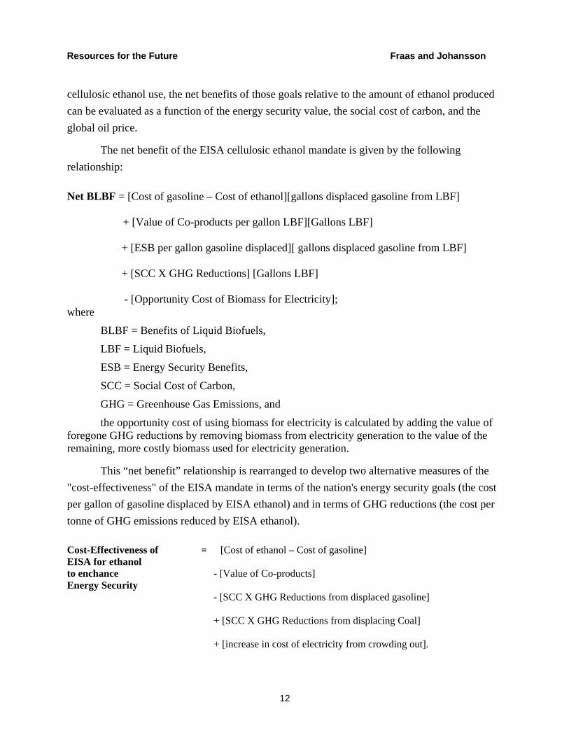
The net benefit of the EISA cellulosic ethanol mandate is given by the following relationship: Net BLBF = [Cost of gasoline – Cost of ethanol][gallons displaced gasoline from LBF]

+ [Value of Co-products per gallon LBF][Gallons LBF]

+ [ESB per gallon gasoline displaced][ gallons displaced gasoline from LBF]

+ [SCC X GHG Reductions] [Gallons LBF] - [Opportunity Cost of Biomass for Electricity]; where

BLBF = Benefits of Liquid Biofuels,

LBF = Liquid Biofuels,

ESB = Energy Security Benefits,

SCC = Social Cost of Carbon,

GHG = Greenhouse Gas Emissions, and

the opportunity cost of using biomass for electricity is calculated by adding the value of foregone GHG reductions by removing biomass from electricity generation to the value of the remaining, more costly biomass used for electricity generation.

This “net benefit” relationship is rearranged to develop two alternative measures of the "cost-effectiveness" of the EISA mandate in terms of the nation's energy security goals (the cost per gallon of gasoline displaced by EISA ethanol) and in terms of GHG reductions (the cost per tonne of GHG emissions reduced by EISA ethanol). Cost-Effectiveness of = [Cost of ethanol – Cost of gasoline] EISA for ethanol to enchance - [Value of Co-products] Energy Security - [SCC X GHG Reductions from displaced gasoline]

+ [SCC X GHG Reductions from displacing Coal] + [increase in cost of electricity from crowding out].


13

Similarly, an alternative cost-effectiveness relationship is developed to reflect the effectiveness of the EISA mandate for cellulosic ethanol in reducing CO2 emissions:

Cost-Effectiveness of = {[Cost of ethanol – Cost of gasoline] EISA ethanol reducing GHG emissions - [ESB per gallon gasoline displaced]

- [Value of Co-products]

+ [Cost of Carbon/Electricity Sector]

X [GHG Reductions from displacing Coal]

+ [increase in cost of electricity from crowding out]} ÷ tonnes of GHG reductions from ethanol displacing gasoline.

This approach allows an assessment of the sensitivity of the cost-effectiveness of the EISA mandate to various factors with a particular focus on the world price of oil and the opportunity cost of foregoing reductions in GHG emissions from the electric utility sector.24 The C-E equation for GHG reductions assumes that a separate regulatory arrangement is in place (i.e., cap-and-trade) for the electric utility sector. Thus, the cost of carbon in the utility sector is exogenous to the transportation sector. Ranges for the determining parameters are described below.

24 Example calculations are provided in Appendix C.


14

World Price of Oil and Cost of Gasoline

Table 1 provides several projections for the world price of oil for the period 2015 to 2025.

Table 1. Projections of World Oil Prices (2007$ per barrel)

2015 2020 2025

AEO2009 (reference case) 110 115 122

AEO2008 (reference case) 61 61 66

DB 72 66 68

IHSGI 98 75 71

IEA 100 110 116

IER 67 70 72

EVA 75 95 105

SEER 98 90 82 Note: EIA, Annual Energy Outlook 2009, Table 16, p. 88. DB: Deutsche Bank. IHGSI: IHS Global Insight, Inc. IEA: International Energy Agency. IER: Institute of Energy Economics and the Rational Use of Energy at the University of Stuttgart. EVA: Energy Ventures Analysis, Inc. SEER: Strategic Energy and Economic Research, Inc.

Data presented by the International Energy Agency (IEA) suggest the following relationship between the world price of oil ($/bbl) and the wholesale price of gasoline ($ per liter gasoline equivalent [lge]): Wholesale Price of Gasoline = 0.01 X [World Price of Oil] - $0.10

Cost of Producing Cellulosic Ethanol

IEA reports a current cost of production for cellulosic ethanol of roughly $ 1.00/lge; but, IEA also reports that in 10 years the cost is projected to be roughly half of the current cost. 25 A

25 IEA, IEA Energy Technology Essentials (January 2007), Table I, p.4.


15

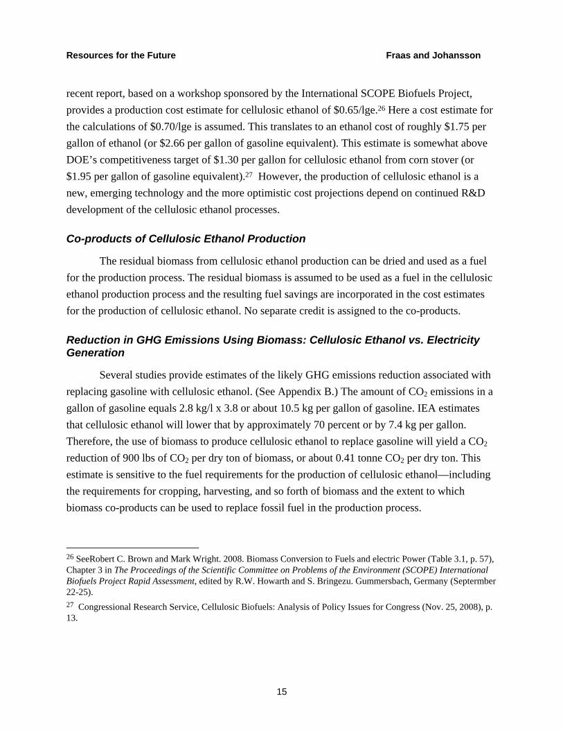
recent report, based on a workshop sponsored by the International SCOPE Biofuels Project, provides a production cost estimate for cellulosic ethanol of $0.65/lge.26 Here a cost estimate for the calculations of $0.70/lge is assumed. This translates to an ethanol cost of roughly $1.75 per gallon of ethanol (or $2.66 per gallon of gasoline equivalent). This estimate is somewhat above DOE’s competitiveness target of $1.30 per gallon for cellulosic ethanol from corn stover (or $1.95 per gallon of gasoline equivalent).27 However, the production of cellulosic ethanol is a new, emerging technology and the more optimistic cost projections depend on continued R&D development of the cellulosic ethanol processes.

Co-products of Cellulosic Ethanol Production

The residual biomass from cellulosic ethanol production can be dried and used as a fuel for the production process. The residual biomass is assumed to be used as a fuel in the cellulosic ethanol production process and the resulting fuel savings are incorporated in the cost estimates for the production of cellulosic ethanol. No separate credit is assigned to the co-products.

Reduction in GHG Emissions Using Biomass: Cellulosic Ethanol vs. Electricity Generation

Several studies provide estimates of the likely GHG emissions reduction associated with replacing gasoline with cellulosic ethanol. (See Appendix B.) The amount of CO2 emissions in a gallon of gasoline equals 2.8 kg/l x 3.8 or about 10.5 kg per gallon of gasoline. IEA estimates that cellulosic ethanol will lower that by approximately 70 percent or by 7.4 kg per gallon. Therefore, the use of biomass to produce cellulosic ethanol to replace gasoline will yield a CO2 reduction of 900 lbs of CO2 per dry ton of biomass, or about 0.41 tonne CO2 per dry ton. This estimate is sensitive to the fuel requirements for the production of cellulosic ethanol—including the requirements for cropping, harvesting, and so forth of biomass and the extent to which biomass co-products can be used to replace fossil fuel in the production process.

26 SeeRobert C. Brown and Mark Wright. 2008. Biomass Conversion to Fuels and electric Power (Table 3.1, p. 57), Chapter 3 in The Proceedings of the Scientific Committee on Problems of the Environment (SCOPE) International Biofuels Project Rapid Assessment, edited by R.W. Howarth and S. Bringezu. Gummersbach, Germany (Septermber 22-25). 27 Congressional Research Service, Cellulosic Biofuels: Analysis of Policy Issues for Congress (Nov. 25, 2008), p. 13.


16

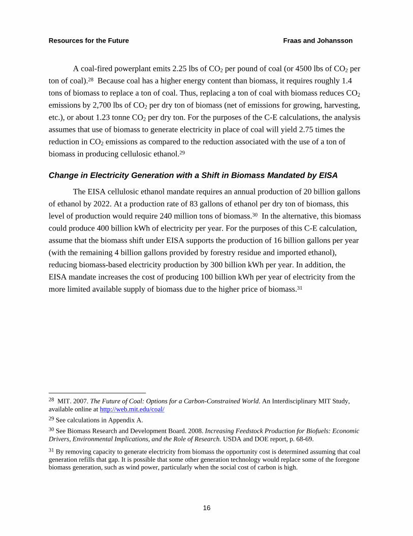
A coal-fired powerplant emits 2.25 lbs of CO2 per pound of coal (or 4500 lbs of CO2 per ton of coal).28 Because coal has a higher energy content than biomass, it requires roughly 1.4 tons of biomass to replace a ton of coal. Thus, replacing a ton of coal with biomass reduces CO2 emissions by 2,700 lbs of CO2 per dry ton of biomass (net of emissions for growing, harvesting, etc.), or about 1.23 tonne CO2 per dry ton. For the purposes of the C-E calculations, the analysis assumes that use of biomass to generate electricity in place of coal will yield 2.75 times the reduction in CO2 emissions as compared to the reduction associated with the use of a ton of biomass in producing cellulosic ethanol.29

Change in Electricity Generation with a Shift in Biomass Mandated by EISA

The EISA cellulosic ethanol mandate requires an annual production of 20 billion gallons of ethanol by 2022. At a production rate of 83 gallons of ethanol per dry ton of biomass, this level of production would require 240 million tons of biomass.30 In the alternative, this biomass could produce 400 billion kWh of electricity per year. For the purposes of this C-E calculation, assume that the biomass shift under EISA supports the production of 16 billion gallons per year (with the remaining 4 billion gallons provided by forestry residue and imported ethanol), reducing biomass-based electricity production by 300 billion kWh per year. In addition, the EISA mandate increases the cost of producing 100 billion kWh per year of electricity from the more limited available supply of biomass due to the higher price of biomass.31

28 MIT. 2007. The Future of Coal: Options for a Carbon-Constrained World. An Interdisciplinary MIT Study, available online at http://web.mit.edu/coal/ 29 See calculations in Appendix A. 30 See Biomass Research and Development Board. 2008. Increasing Feedstock Production for Biofuels: Economic Drivers, Environmental Implications, and the Role of Research. USDA and DOE report, p. 68-69. 31 By removing capacity to generate electricity from biomass the opportunity cost is determined assuming that coal generation refills that gap. It is possible that some other generation technology would replace some of the foregone biomass generation, such as wind power, particularly when the social cost of carbon is high.


17

Increase in Cost of Electricity Production

This C-E calculation assumes that the EISA mandate results in a $0.005/kWh increase in the cost of electricity for both the replacement generation (300 kWh/year) and for the residual biomass generated electricity (100 kWh/year).32

Results

Using the values and assumptions outlined above, the following estimates for the cost-effectiveness of the EISA mandate as a function of the world oil price and SCC are developed for several alternative scenarios:

1. World price of oil at $40/bbl, $70/bbl, $100/bbl, and

2. SCC at $10, $40, and $70 per tonne of CO2.33

Cost-Effectiveness in Terms of Energy Supply

EPA’s recent analysis of the EISA cellulosic mandate considers a scenario based on the annual production of 16 billion gallons of cellulosic ethanol in 2022.34 This level of production will require roughly 200 million dry tons of biomass and would represent a substantial fraction of the projected biomass production in 2020. At this level of production, the cellulosic ethanol requirements of EISA would compete with the use of biomass to generate electricity, giving rise to an opportunity cost to the EISA cellulosic ethanol mandate. However, as discussed above, Section 202(e) of EISA allows the Administrator of EPA to adjust the mandated volume. In its

32 See EIA. 2009. Energy Market and Economic Impacts of H.R. 2454, the American Clean Energy and Security Act of 2009. Table 1. Report No. SR/OIAF/2009-05 (August): 10. In 2020, the credit price—reflecting the marginal cost of renewable generation—is $0.006 per kwh for the less stringent of the renewable electricity standard scenarios. The increase in renewable generation in this scenario is based on an increase in the use of biomass to generate electricity. In 2020, the credit price—reflecting the marginal cost of renewable generation—is $0.006 per kwh for the less stringent of the renewable electricity standard scenarios. The increase in renewable generation in this scenario is based on an increase in the use of biomass to generate electricity. 33 In its recent final CAFE rule, DOT employed a range of estimates to reflect the uncertainty surrounding the value of the Social Cost of Carbon: a domestic value of $2 per tonne of CO2; a global value of $33 per tonne of CO2 [the mean value in Tol (2008)]; and, a global value of $80 per tonne of CO2 (one standard deviation above the mean value for Tol). Department of Transportation; NHTSA; Average Fuel Economy Standards, Passenger Cars and Light Trucks, Model Year 2011. Final Rule. Federal Register 74: 14195–14456, March 30. 34 U.S. Environmental Protection Agency (EPA). Regulation of Fuels and Fuel Additives: Changes to Renewable Fuel Standard Program. Proposed Rule. Federal Register 74: 24904–25143, May 26. For this scenario, EPA assumes that the U.S. will import the additional ethanol required to meet the EISA mandate in 2022.


18

recent 2009 AEO, EIA projects a level of cellulosic ethanol production of only 5 billion gallons per year in 2022 based on its projection of a much slower expansion of cellulosic ethanol production capacity than required by the volumes specified by EISA. Under this scenario, EPA would adjust the mandated volumes for cellulosic ethanol in the period from 2016 through at least 2022, substantially reducing the competition for biomass from the biofuel sector.35

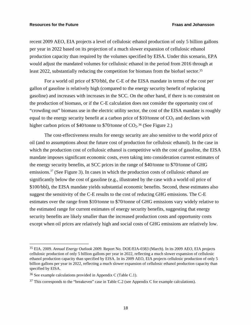
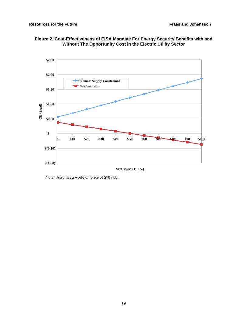
For a world oil price of $70/bbl, the C-E of the EISA mandate in terms of the cost per gallon of gasoline is relatively high (compared to the energy security benefit of replacing gasoline) and increases with increases in the SCC. On the other hand, if there is no constraint on the production of biomass, or if the C-E calculation does not consider the opportunity cost of “crowding out” biomass use in the electric utility sector, the cost of the EISA mandate is roughly equal to the energy security benefit at a carbon price of $10/tonne of CO2 and declines with higher carbon prices of $40/tonne to $70/tonne of CO2.36 (See Figure 2.)

The cost-effectiveness results for energy security are also sensitive to the world price of oil (and to assumptions about the future cost of production for cellulosic ethanol). In the case in which the production cost of cellulosic ethanol is competitive with the cost of gasoline, the EISA mandate imposes significant economic costs, even taking into consideration current estimates of the energy security benefits, at SCC prices in the range of $40/tonne to $70/tonne of GHG emissions.37 (See Figure 3). In cases in which the production costs of cellulosic ethanol are significantly below the cost of gasoline (e.g., illustrated by the case with a world oil price of $100/bbl), the EISA mandate yields substantial economic benefits. Second, these estimates also suggest the sensitivity of the C-E results to the cost of reducing GHG emissions. The C-E estimates over the range from $10/tonne to $70/tonne of GHG emissions vary widely relative to the estimated range for current estimates of energy security benefits, suggesting that energy security benefits are likely smaller than the increased production costs and opportunity costs except when oil prices are relatively high and social costs of GHG emissions are relatively low.

35 EIA. 2009. Annual Energy Outlook 2009. Report No. DOE/EIA-0383 (March). In its 2009 AEO, EIA projects cellulosic production of only 5 billion gallons per year in 2022, reflecting a much slower expansion of cellulosic ethanol production capacity than specified by EISA. In its 2009 AEO, EIA projects cellulosic production of only 5 billion gallons per year in 2022, reflecting a much slower expansion of cellulosic ethanol production capacity than specified by EISA. 36 See example calculations provided in Appendix C (Table C.1). 37 This corresponds to the “breakeven” case in Table C.2 (see Appendix C for example calculations).


19

Figure 2. Cost-Effectiveness of EISA Mandate For Energy Security Benefits with and Without The Opportunity Cost in the Electric Utility Sector

$(1.00)

$(0.50)

$-

$0.50

$1.00

$1.50

$2.00

$2.50

$- $10 $20 $30 $40 $50 $60 $70 $80 $90 $100

SCC ($/MTCO2e)

CE

($/g

al)

Biomass Supply ConstrainedNo Constraint

Note: Assumes a world oil price of $70 / bbl.


20

Figure 3. Cost-Effectiveness of the EISA Mandate (Cost per Gallon of Gasoline Displaced)

-$1.00

-$0.50

$0.00

$0.50

$1.00

$1.50

$2.00

$2.50

$3.00

$3.50

$0 $20 $40 $60 $80 $100 $120

SCC ($MTCO2e)

CE

($/g

allo

n)

$40/bbl $70/bbl $100/bblES-low ES-med ES-high

Note: “ES-low”, “ES-med”, and “ES-high” correspond to the low ($0.12 per gallon), medium ($0.30 per gallon), and high ($0.50 per gallon) ranges chosen by DOT to represent ranges of the value of energy security.38

Cost-Effectiveness of Lowering CO2 Emissions

The calculation of the cost-effectiveness per gallon of gasoline displaced by ethanol is sensitive to assumptions about world oil prices and the cost of producing cellulosic ethanol. (See Figure 4). At a world oil price of $70/bbl, the EISA cellulosic ethanol mandate yields a very expensive reduction in CO2 emissions from the transportation sector. On the other hand, at a

38See Department of Transportation (DOT). 2008. Average Fuel Economy Standards, Passenger Cars and Light Trucks; Model Years 2011-2015. Proposed Rule. Federal Register 73: 24352–24487, May 2. Also see Department of Transportation; NHTSA; Average Fuel Economy Standards, Passenger Cars and Light Trucks, Model Year 2011. Final Rule. Federal Register 74: 14195–14456, March 30.


21

world oil price of $100/bbl, the ethanol mandate yields a cost-effective reduction in CO2 emissions up to a carbon allowance price of roughly $90/tonne in the electric utility sector.39

Figure 4. Cost–Effectiveness of GHG Emission Control (Cost per Tonne of CO2 Reduced)

Caveats

A key factor not reflected in the illustrations above is that the basic elements for burning biomass for energy are well known—wood has served as an energy source from the beginning of history. Biomass can be used to generate electricity at a cost that is roughly comparable to that for coal. There are no technological breakthroughs required to use biomass to raise steam to generate electricity. In addition, the infrastructure necessary to generate and deliver electricity is already in place. There is little additional retrofit required to co-fire pelletized biomass in existing coal-fired plants, and these plants are already connected to the grid. On the other hand,

39 See example calculations of the cost-effectiveness of reducing GHG emissions using ethanol in Appendix C (Table C.3).


22

as discussed below, the conversion of biomass to liquid biofuels still requires a significant R & D program in order to be competitive with gasoline and with corn- and sugar-derived ethanol.

There are still hurdles to the use of biomass to generate electricity in dedicated power plants. The biomass required to fuel an electric power plant will require the development of significant energy plantation agriculture. For example, the scale for an energy plantation for co-firing biomass at a 1000 MW coal-fired power plant would be on the order of 20 to 40 square miles. This will require the development and implementation of new technologies for cropping and harvesting biomass and the transportation of the bulky biomass to the plant. 40 Over time it is also likely that biomass yields per acre will increase, which could mitigate to a certain degree constraints on biomass supply.

There are even more substantial hurdles to the conversion of cellulosic biomass to liquid biofuels on the scale required by the EISA mandate. Foremost of these—as noted above--is the additional R & D required to yield processes that are cost-competitive with gasoline and other sources of ethanol. It may be to meet goals for increasing cellulosic ethanol use, when biomass supply is constrained, that the U.S. will have to substantially increase imports of ethanol. Ethanol imports may become progressively cheaper if the cost of acquiring biomass rises and pushes up the cost of producing ethanol domestically. However, it is unclear which types of ethanol could be imported to satisfy the lifecycle requirements of the renewable fuels standard and the extent to which international supply could be increased for U.S. consumption.

There are potential "upsides" in a successful R&D program in terms of cost reductions, energy savings, and reductions in GHG emissions that are not reflected in the illustrative calculations presented above. In particular, EPA projected substantial absolute reductions in GHG emissions with the production of switchgrass-based cellulosic ethanol in its lifecycle analysis for its recent proposed rule for the Renewable Fuel Standard Program. These projections are based on the assumption that switchgrass residues will be used in a cogeneration facility to

40 There have been problems at pilot scale plants with the reliability of the processing equipment which tend to jam when converting biomass to a usable fuel for the powerplant. This processing equipment is expensive and, if the jamming problem cannot be solved, plants will have to install spare capacity in order to maintain a continuous supply of fuel. EIA, Energy and Economic Impacts of Implementing Both a 25-Percent RPS and a 25-Percent RFS by 2025, September 2007, pp. 8-9.


23

meet the energy requirements of the cellulosic ethanol plant and generate excess electricity for sale to the grid (displacing fossil-fuels).41

Beyond the R & D requirements, the conversion of cellulosic biomass to ethanol requires a substantially more capital intensive process than those processes using corn and sugar as a feedstock. Current estimates are that a cellulosic ethanol plant will cost $300 million—four times the cost of a plant that produces corn-derived ethanol. The capital investment required for these plants—especially in the current investment climate—will serve as a significant barrier to meeting the EISA mandate.

There are other significant capital requirements, as well—requirements that cellulosic ethanol shares with corn- and sugar-derived ethanol. Because of the affinity of ethanol for water and the corrosive nature of ethanol/water mixtures for the current oil and gasoline pipeline infrastructure , the transportation of ethanol and ethanol blends is currently limited to truck, rail, and barge transportation. To handle the volume of ethanol required by the EISA mandate, a distribution infrastructure that is ethanol tolerant must be developed—one that may require a new pipeline system dedicated to ethanol.

In addition, the current fleet of U.S. vehicles is designed to be fueled with a gasoline/ethanol blend containing no more than 10 percent ethanol. Thus, ethanol use by the current fleet of cars and trucks cannot under current conditions exceed more than 10 percent of current gasoline consumption—roughly 14 BGY—creating the so-called “blend wall.”42 As a short term solution, EPA may be able to certify that the current fleet could tolerate ethanol blends containing 15 percent ethanol (or even 20 percent ethanol, as requested by Minnesota).43 If the United States is to use the volumes required by the EISA mandate, the longer term solution—the development of a distribution infrastructure and a vehicle fleet that can run off a gasoline-ethanol blends of up to 85 percent ethanol, or E85—will require a substantial additional capital investment.

41 See U.S. Environmental Protection Agency (EPA). Regulation of Fuels and Fuel Additives: Changes to Renewable Fuel Standard Program. Proposed Rule. Federal Register 74: 24904–25143, May 26. 42 U.S. Environmental Protection Agency (EPA). Regulation of Fuels and Fuel Additives: Changes to Renewable Fuel Standard Program. Proposed Rule. Federal Register 74: 24904–25143, May 26. 43 U.S. Environmental Protection Agency (EPA). Notice of Receipt of a Clean Air Act Waiver Application to Increase the Allowable Ethanol Content of Gasoline to 15 Percent; Request for Comment. Federal Register 74: 18228–18230, April 21.


24

Finally, a decision by the EPA Administrator to relax the mandates on cellulosic ethanol use, in response to either a state petition or to a shortfall in available volumes of cellulosic ethanol, will reduce the demand for biomass, relaxing the biomass constraint. As a result, a reduced mandate for the use of cellulosic ethanol would alter the calculations of cost-effectiveness.

Conclusion

This paper identifies some of the key factors that affect the cost-effectiveness of using biomass to produce liquid biofuels as required by the EISA cellulosic ethanol mandate. Current estimates/projections suggest that biomass has a comparative advantage in reducing greenhouse gases when used to generate electricity (in place of coal) instead of producing cellulosic ethanol to displace gasoline. On the other hand, use of biomass to produce cellulosic ethanol also enhances energy security in the United States, a goal of the EISA legislation.

As an initial matter, the opportunity cost of diverting biomass from the electric utility sector to the production of cellulosic ethanol substantially affects the cost-effectiveness evaluation of the program. If the supply of biomass available in the 2020 to 2025 period is sufficient to meet the EISA mandate without crowding out biomass use to generate electricity, then the EISA mandate would appear to be a cost-effective policy for the scenarios evaluated above. On the other hand, if the EISA mandate crowds out the use of biomass to generate electricity, then it may significantly increase GHG emissions associated with electricity generation from coal-fired power plants. EISA requires EPA to consider the “direct and significant indirect emissions” of biofuels in determining eligibility for the program. Given the potential crowding out of the use of biomass in place of coal to generate electricity, EPA’s evaluation should include any potential increase in GHG emissions in the electric utility sector associated with the shift of biomass into the production of cellulosic ethanol.44

More importantly, the analysis in this paper suggests that the cost-effectiveness of the EISA mandate as an energy security measure varies substantially with world oil prices (and/or changes in the price spread between gasoline and the production cost of cellulosic ethanol) and with different values for the cost of carbon. Similarly, the cost-effectiveness of the EISA

44 Note that if Congress adopts a cap-and-trade program limiting GHG emissions from the electric utility sector, a cost-effectiveness evaluation of EISA should still include a consideration of the potential increase in generation costs in the electric utility.


25

mandate—including the opportunity cost of diverting biomass away from the generation of electricity—varies substantially with the cost of carbon control in the electric utility sector. As a result, energy security benefits are likely a smaller factor in determining the benefits and costs of the EISA mandate for cellulosic ethanol as compared to other factors except in the case when the world price of oil is relatively high and the social cost of carbon is relatively low.

For the illustrative set of scenarios presented here, the EISA cellulosic ethanol mandate would not be cost-effective at world oil prices less than roughly $80 per barrel. At world oil prices greater than $100 per barrel, the mandate would be irrelevant because market forces would yield cellulosic ethanol production levels that exceed the EISA mandate levels. In general, the EISA mandate will be cost-effective if (1) there is a supply of biomass that is sufficient to meet the low-cost fuel supply requirements of both the electric utility sector and the EISA mandate for cellulosic ethanol or if (2) the world oil price is greater than $100 per barrel and the production costs for cellulosic ethanol are less than $2 per gallon. The EISA mandate will not be cost-effective if (1) biomass supply is limited so that EISA crowds out the use of biomass by the electric utility sector and if (2) world oil prices are less than $80 per barrel (at cellulosic ethanol prices of $2 per gallon).

One way of accomplishing a level playing field is to incorporate energy security fees for petroleum products and CO2 emission fees across fuels and energy production activities. Once these fees are set, the market can determine the best mix of fuels and technologies to obtain the nation’s expected energy security and GHG reduction goals. Artificial constraints on the market economy—such as mandated volumes for biofuels—can interfere with its ability to determine the most cost-effective means to achieve energy security and GHG reductions. Those constraints can impose costs on the economy in addition to the already large costs anticipated from an optimal set of climate and energy policies.


26

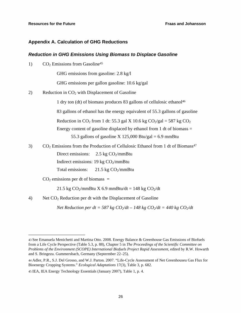
Appendix A. Calculation of GHG Reductions

Reduction in GHG Emissions Using Biomass to Displace Gasoline

1) CO2 Emissions from Gasoline45

GHG emissions from gasoline: 2.8 kg/l

GHG emissions per gallon gasoline: 10.6 kg/gal

2) Reduction in CO2 with Displacement of Gasoline

1 dry ton (dt) of biomass produces 83 gallons of cellulosic ethanol46

83 gallons of ethanol has the energy equivalent of 55.3 gallons of gasoline

Reduction in CO2 from 1 dt: 55.3 gal X 10.6 kg CO2/gal = 587 kg CO2

Energy content of gasoline displaced by ethanol from 1 dt of biomass =

55.3 gallons of gasoline X 125,000 Btu/gal = 6.9 mmBtu

3) CO2 Emissions from the Production of Cellulosic Ethanol from 1 dt of Biomass47

Direct emissions: 2.5 kg CO2/mmBtu

Indirect emissions: 19 kg CO2/mmBtu

Total emissions: 21.5 kg CO2/mmBtu

CO2 emissions per dt of biomass =

21.5 kg CO2/mmBtu X 6.9 mmBtu/dt = 148 kg CO2/dt

4) Net CO2 Reduction per dt with the Displacement of Gasoline

Net Reduction per dt = 587 kg CO2/dt – 148 kg CO2/dt = 440 kg CO2/dt

43 See Emanuela Menichetti and Martina Otto. 2008. Energy Balance & Greenhouse Gas Emissions of Biofuels from a Life Cycle Perspective (Table 5.3, p. 88), Chapter 5 in The Proceedings of the Scientific Committee on Problems of the Environment (SCOPE) International Biofuels Project Rapid Assessment, edited by R.W. Howarth and S. Bringezu. Gummersbach, Germany (Septermber 22–25). 44 Adler, P.R., S.J. Del Grosso, and W.J. Parton. 2007. “Life-Cycle Assessment of Net Greenhouseu Gas Flux for Bioenergy Cropping Systems.” Ecological Adaptations 17(3), Table 3, p. 682. 45 IEA, IEA Energy Technology Essentials (January 2007), Table 1, p. 4.


27

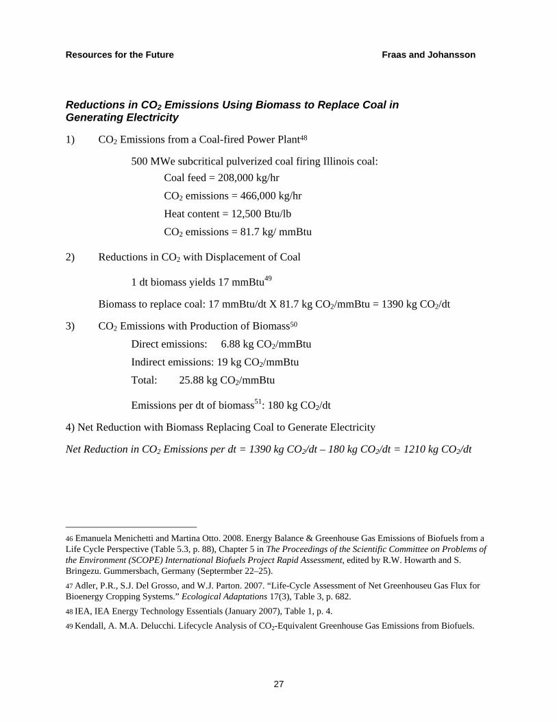
Reductions in CO2 Emissions Using Biomass to Replace Coal in Generating Electricity

1) CO2 Emissions from a Coal-fired Power Plant48

500 MWe subcritical pulverized coal firing Illinois coal: Coal feed = 208,000 kg/hr

CO2 emissions = 466,000 kg/hr

Heat content = 12,500 Btu/lb

CO2 emissions = 81.7 kg/ mmBtu

2) Reductions in CO2 with Displacement of Coal 1 dt biomass yields 17 mmBtu49

Biomass to replace coal: 17 mmBtu/dt X 81.7 kg CO2/mmBtu = 1390 kg CO2/dt

3) CO2 Emissions with Production of Biomass50

Direct emissions: 6.88 kg CO2/mmBtu

Indirect emissions: 19 kg CO2/mmBtu

Total: 25.88 kg CO2/mmBtu Emissions per dt of biomass51: 180 kg CO2/dt

4) Net Reduction with Biomass Replacing Coal to Generate Electricity

Net Reduction in CO2 Emissions per dt = 1390 kg CO2/dt – 180 kg CO2/dt = 1210 kg CO2/dt

46 Emanuela Menichetti and Martina Otto. 2008. Energy Balance & Greenhouse Gas Emissions of Biofuels from a Life Cycle Perspective (Table 5.3, p. 88), Chapter 5 in The Proceedings of the Scientific Committee on Problems of the Environment (SCOPE) International Biofuels Project Rapid Assessment, edited by R.W. Howarth and S. Bringezu. Gummersbach, Germany (Septermber 22–25). 47 Adler, P.R., S.J. Del Grosso, and W.J. Parton. 2007. “Life-Cycle Assessment of Net Greenhouseu Gas Flux for Bioenergy Cropping Systems.” Ecological Adaptations 17(3), Table 3, p. 682. 48 IEA, IEA Energy Technology Essentials (January 2007), Table 1, p. 4. 49 Kendall, A. M.A. Delucchi. Lifecycle Analysis of CO2-Equivalent Greenhouse Gas Emissions from Biofuels.


28

Appendix B. Ethanol GHG Reductions

Author Site/Scope GHG Improvement Feedstock

w/o land-use change52 w/ land-use change

Farrell et al. USA 88% n/a Switchgrass

Quirin et al. Various 15-115% n/a Lignocelluloses

Elsayed et al. Various 84% n/a Wheat straw

Edwards et al. Europe/Brazil 76-88% n/a Wheat straw, wood

Grood/Haywood USA 93-98% n/a Switchgrass

Unnasch/Pont USA 10-102% n/a Poplar, switchgrass

Wang et al. USA 86% n/a Unknown

Veeraraghaven UK 88-98% n/a Wheat straw

Choudhury et al. Europe 70% n/a Poplar

Zah et al. Swiss/Europe 65% n/a Grass/wood

Adler et al.53 USA 115% n/a Grass/wood

IEA54 Various n/a 70% Lignocelluloses

Kendall/Delucchi55 USA n/a 40-75% Not specified

CARB/Low carbon56 USA n/a 78% Wood

52 Column for “w/o land-use change” is adapted from Emanuela Menichetti and Martina Otto. 2008. Energy Balance & Greenhouse Gas Emissions of Biofuels from a Life Cycle Perspective (Table 5.3, p. 88), Chapter 5 in The Proceedings of the Scientific Committee on Problems of the Environment (SCOPE) International Biofuels Project Rapid Assessment, edited by R.W. Howarth and S. Bringezu. Gummersbach, Germany (Septermber 22–25). 53 Adler, P.R., S.J. Del Grosso, and W.J. Parton. 2007. “Life-Cycle Assessment of Net Greenhouseu Gas Flux for Bioenergy Cropping Systems.” Ecological Adaptations 17(3), Table 3, p. 682. 54 IEA. 2007. IEA Energy Technology Essentials. Table 1, p. 1 (January). 55 Kendall, A. M.A. Delucchi. Lifecycle Analysis of CO2-Equivalent Greenhouse Gas Emissions from Biofuels.


29

Appendix C. Example Calculations

Calculation of the C-E of Energy Security

Table C.1 illustrates the C-E estimates of including the opportunity cost of “crowding out” the use of biomass to replace coal in the generation of electricity.

Table C.1. Cost-Effectiveness of EISA Mandate for Energy Security Benefits with and without the Opportunity Cost in the Electric Utility Sector (World Oil Price = $70/bbl)

With opportunity cost Without opportunity cost SCC $10/tonne $0.70/gal $0.31/gal $40/tonne $1.09/gal $0.08/gal $70/tonne $1.48/gal [$0.14/gal]* * For this scenario, the EISA mandate yields net benefits, so that the cost per gallon of gasoline displaced is negative.

An example calculation of the cost-effectiveness for energy security benefits at a world oil price of $70 per bbl and assuming a social cost of carbon of $40 per tonne is:

Cost-effectiveness of = [$0.70/lge - $0.60/lge] x 3.8 l/gallon EISA for ethanol to enhance - [$0/lge] energy security - [$40/tonne x .00742 tonne /gallon] +[$40/tonne x .0204 tonne/gallon]

+ [([$0.005/kwh x 300 billion kwh] + [$0.005/kwh x 100 billion kwh])/ 10.67 billion gallons]

= $1.09 per gallon.

56 California Air Resources Board (CARB), Low Carbon Fuel Standard (2009), p. 5. CARB esitmated a 98% reduction for biofuel displacing gasoline without an adjustment for land-use changes.


30

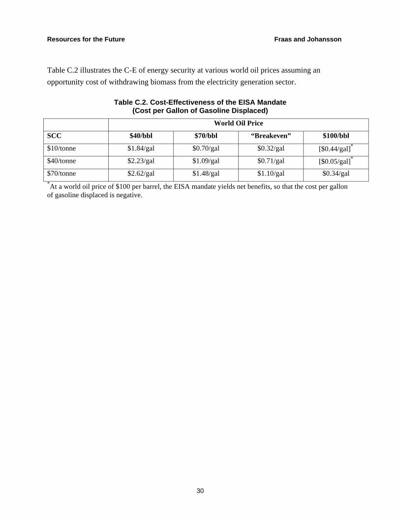
Table C.2 illustrates the C-E of energy security at various world oil prices assuming an opportunity cost of withdrawing biomass from the electricity generation sector.

Table C.2. Cost-Effectiveness of the EISA Mandate (Cost per Gallon of Gasoline Displaced)

World Oil Price

SCC $40/bbl $70/bbl “Breakeven” $100/bbl

$10/tonne $1.84/gal $0.70/gal $0.32/gal [$0.44/gal]*

$40/tonne $2.23/gal $1.09/gal $0.71/gal [$0.05/gal]*

$70/tonne $2.62/gal $1.48/gal $1.10/gal $0.34/gal *At a world oil price of $100 per barrel, the EISA mandate yields net benefits, so that the cost per gallon of gasoline displaced is negative.


31

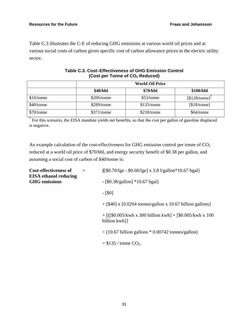
Table C.3 illustrates the C-E of reducing GHG emissions at various world oil prices and at various social costs of carbon given specific cost of carbon allowance prices in the electric utility sector.

Table C.3. Cost–Effectiveness of GHG Emission Control (Cost per Tonne of CO2 Reduced)

World Oil Price $40/bbl $70/bbl $100/bbl $10/tonne $206/tonne $53/tonne [$128/tonne]* $40/tonne $289/tonne $135/tonne [$18/tonne]

$70/tonne $371/tonne $218/tonne $64/tonne * For this scenario, the EISA mandate yields net benefits, so that the cost per gallon of gasoline displaced is negative.

An example calculation of the cost-effectiveness for GHG emission control per tonne of CO2 reduced at a world oil price of $70/bbl, and energy security benefit of $0.38 per gallon, and assuming a social cost of carbon of $40/tonne is: Cost-effectiveness of = {[$0.70/lge - $0.60/lge] x 3.8 l/gallon*10.67 bgal] EISA ethanol reducing GHG emissions - [$0.38/gallon] *10.67 bgal]

- [$0]

+ [$40] x [0.0204 tonnes/gallon x 10.67 billion gallons]

+ [([$0.005/kwh x 300 billion kwh] + [$0.005/kwh x 100 billion kwh]}

÷ (10.67 billion gallons * 0.00742 tonnes/gallon) = $135 / tonne CO2.

august 2009 rff dp 09-24 discussion paper

Documents