arapier - a fortran iv program for multiple linear regression … · analysis providing internally...

,-. 0

NASA TECHNICAL N O T E NASA ID-5656- TN f

RAPIER - A FORTRAN IV PROGRAM FOR MULTIPLE LINEAR REGRESSION ANALYSIS PROVIDING INTERNALLY EVALUATED REMODELING

by Steven M . Sidik und Bert Henry

Lewis Reseurch Center , 1

.:Y i' L.

NATIONAL A E R O N A U T I C S AND S P A C E ADMINISTRATION WASHINGTON, D. c . F E B R U A R Y 1970

https://ntrs.nasa.gov/search.jsp?R=19700009705 2019-02-14T06:23:24+00:00Z

- - -

TECH LIBRARY KAFB, NM

llllllllllllllllllllllllllllllllllllliill1111 1. Report No. 2. Government Accession No.

NASA TN D-5656 I 4. T i t l e and Subtit le RAPIER - A FORTRAN IV PROGRAM

FOR MULTIPLE LINEAR REGRESSION ANALYSIS PROVIDING INTERNALLY EVALUATED REMODE LING

7. Author(s) Steven M. Sidik and Bert Henry

9. Performing Organizotion Name and Address

Lewis Research Center National Aeronautics and Space Administration Cleveland, Ohio 44135

2. Sponsoring Agency Name and Address

National Aeronautics and Space Administration Washington, D. C. 20546

'5. Supplementary Notes

16. Abstroci

01325LL3. Recipient 's Catalog No.

5. Report Dote Februarv 1970

6. Performing Organization Code

0. Performing Organization Report No. E-4748

10. Work Un i t No. 129-04

11. Controct or Grant No.

13. Type of Report and Per iod Covered

Technical Note

14. Sponsoring Agency Code

RAPIER is a very flexible, easy to use, sophisticated multiple l inear regression p r o g r m which computes the variance-covariance matrix of the independent variables, regression coefficients, t-statistics for individual tests, and analysis of variance tables. The major value of the program is its comprehensiveness and options, such a s a choice of t h ree s t ra tegies for the variance estimate, a n analysis of more than one set of response variables for the same independent variables, a backward rejection based on the first response variable, the use of weighted regression, computation of predicted values for any combination of independent variables, and a chi-square test for normality.

17. Key Words (Suggested by Author ( s ) ) 18. Distr ibut ion Statement

Multiple regression Unclassified - unlimited Least squares Curve fitting

19. Security Classif. (of t h i s report) 20. Security Classif. (of this page) 1 21. No. of Pages I 22. P r i c e *

Unclassified Unclassified 87 $3.00

CONTENTS

Page SUMMARY . . . . . . . . . . . . . . . . . . . . . . . . . . . . . . . . . . . . . . . 1

INTRODUCTION . . . . . . . . . . . . . . . . . . . . . . . . . . . . . . . . . . . . 1

SYMBOLS . . . . . . . . . . . . . . . . . . . . . . . . . . . . . . . . . . . . . . . 2

ESTIMATION OF BASIC LINEAR MODEL . . . . . . . . . . . . . . . . . . . . . . 5 Basic Linear Model . . . . . . . . . . . . . . . . . . . . . . . . . . . . . . . . . 5 Estimating b . . . . . . . . . . . . . . . . . . . . . . . . . . . . . . . . . . . . 8 Correlation Matrix . . . . . . . . . . . . . . . . . . . . . . . . . . . . . . . . . 10 Estimating u2 . . . . . . . . . . . . . . . . . . . . . . . . . . . . . . . . . . . 11

HYPOTHESIS TESTING . . . . . . . . . . . . . . . . . . . . . . . . . . . . . . . . 12 Test NE .Normality of e . . . . . . . . . . . . . . . . . . . . . . . . . . . . . 12 Analysis of Variance Table . . . . . . . . . . . . . . . . . . . i . . . . . . . . . 15 Choice of Estimator for u2 . . . . . . . . . . . . . . . . . . . . . . . . . . . . 16 Test OR .Overall Regression . . . . . . . . . . . . . . . . . . . . . . . . . . . 17 Test S F .Sequential F-Test . . . . . . . . . . . . . . . . . . . . . . . . . . . . 17 Test TT .t-Tests . . . . . . . . . . . . . . . . . . . . . . . . . . . . . . . . . 18

PREDICTING VALUES FROM ESTIMATED REGRESSION EQUATION . . . . . . . 19

USER'S GUIDE TO INPUT . . . . . . . . . . . . . . . . . . . . . . . . . . . . . . 20 Sample Regression Problem . . . . . . . . . . . . . . . . . . . . . . . . . . . . 20 Types of Input Cards . . . . . . . . . . . . . . . . . . . . . . . . . . . . . . . . 22

SAMPLE OUTPUT . . . . . . . . . . . . . . . . . . . . . . . . . . . . . . . . . . 33

APPENDIXES A .PROGRAM DOCUMENTATION AND LISTINGS . . . . . . . . . . . . . . . . 46 B .BORROWED ROUTINES . . . . . . . . . . . . . . . . . . . . . . . . . . . . 85

REFERENCES . . . . . . . . . . . . . . . . . . . . . . . . . . . . . . . . . . . . . 87

iii

.......

RAPIER - A FORTRAN I V PROGRAM FOR MULTIPLE LINEAR REGRESSION

ANALYSIS PROVIDING INTERNALLY EVALUATED REMODELING

by Steven M. Sidik and Bert Henry

Lewis Research Center

SUMMARY

RAPIER is a digital computer program which can be used with ease to perform extensive regression analyses or a simple least-squares curve fit, and it includes a backward te rm rejection option. The program is written in FORTRAN IV, version 13, for the IBM 7094/7044 DCS. The major value of the program is its comprehensiveness of calculations and options.

RAPIER computes the variance-covariance matrix of the independent variables, regression coefficients, t-statistics for individual tests, and analysis of variance tables for overall testing of regression. There is a provision for a choice of three strategies for the variance estimate to be used in computing t-statistics.

Also, more than one set of response or dependent variables can by analyzed for the same set of independent variables.

A backward rejection option method based on the first dependent variable may be used. In this case, a critical significance level is supplied as input. The least significant independent variable is deleted and the regression recomputed. This process is repeated until all remaining variables have significantly nonzero coefficients.

The algorithm uses the triangular form of symmetric matrices throughout. It also allows for the use of weighted regression, computation of predicted values at any combination of independent variables, a table of residuals, and a chi-square test for the normality of the distribution of residuals.

I NTROD UCTlON

RAPIER is an almost entirely new multiple regression computer program. It is the result of 5 years of development in meeting the needs of several statistical investigators posing a variety of problems. The problems included analysis of nuclear reactor components, determining predictive models from corrosion and fracture data of both metals and alloys, investigating the behavior of processing variables in the manufacture of

solar cells, optimizing fuel-cell experiment procedures, and predicting personnel performance from academic histories.

The nucleus of the program is based on a program written by Kunin (ref. 1). However, in its present expanded form, it allows the user to choose from a number of sets of options which- include options of input, of methods for calculation, and of output, thereby providing great flexibility.

With the aid of a few control cards, the program can be used readily for a wide range of applications which can vary from a simple least-squares curve-fitting problem to a complete regression analysis. It can provide the variance-covariance matrix of independent variables, regression coefficients, the variance-covariance matrix of the regression coefficients, individual t-statistics with their significance levels, analysis of variance tables ior significance of regression, special usage of replicated data to estimate the e r r o r d w to lack of fit, any one of three pooling procedures which may be used to estimate the e r ro r variance, tests for normality of distribution of the residuals, weighted regression, and the use of more than one dependent variable.

The mathematical analysis of the computations and their reliability is aided further by the option of obtaining an eigenvector decomposition of both the variance-covariance matrix and the correlation matrix of the independent variables.

The program also provides an option to perform a backward rejection regression at any given level of significance.

Despite its sophistication, RAPIER is relatively easy to use, but it presupposes that the user has at least a basic knowledge and/or experience in the application of statistical techniques.

To provide a framework for the discussion of the calculations and statistical options available in RAPIER, a brief description of multiple linear regression is presented, with no attempt to make the discussion thorough or rigorous. Notable presentations of applied regression analysis a r e those by Draper and Smith (ref. 2) and Graybill (ref. 3). Reference 4 by Kendall and Stuart is a useful guide to both applications and theoretical justifications. Rao (ref. 5) presents a more mathematically sophisticated treatment of the subject of linear statistical models.

After discussion of the calculations and options available, the card input necessary is described in detail and illustrated by an example which uses almost all of the options.

SYMBOLS

A matrix

A' transpose of A

A - ~ inverse of A

2

B

b

bi*

bi

b l ,

C

C..9 D

E(XI

e

Fa, b

f

fj(Z1'

HO

H1 J

K

k

LOF

M

matrix

vector (column)

t rue regression coefficient

estimated regression coefficient

constant te rm

' - 9 bJ unknown parameters

correlation matrix

elements of C

indicator variable, equal to 0 if no bo coefficient is estimated and equal to 1 if bo is estimated

expected value of x (i. e., average of x over all possible values of x)

vector of observation e r r o r s

statistic distributed as variance ratio with a and b degrees of freedom

expected number of observations in each cell of a partitioned range of studentiz ed residuals

. . ., zK) t e rm of regression equation

statistical hypothesis to be tested

alternate hypothesis to be accepted if Ho is judged to be false

number of coefficients estimated, excluding bo

number of independent variables observed

number of segments or cells in range of possible studentized residuals

lack of f i t

total number of independent and dependent variables

' MS(source) mean square due to source, where source is REG, RES, etc.

m moment about origin

N number of observations

N ( P P2) normal distribution with mean p and variance u2

ni number of studentized residuals in ith cell

3

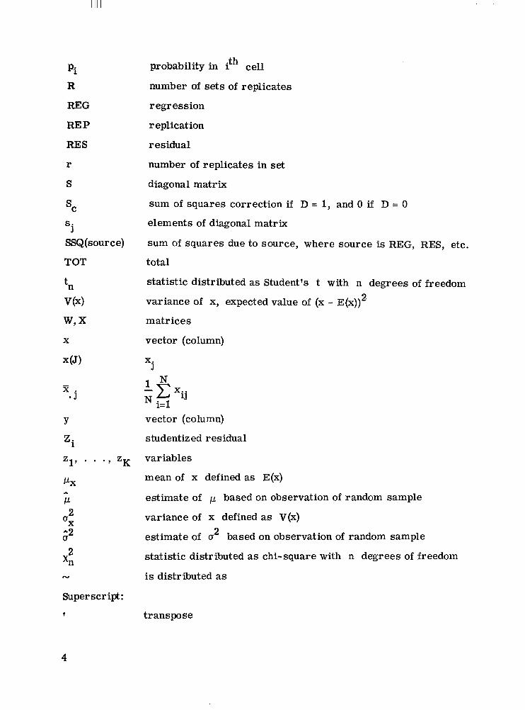
Pi probability in ith cell

R number of sets of replicates

REG regression

REP replication

RES residual

r number of replicates in set

S diagonal matrix

sC sum of squares correction if D = 1, and 0 if D = 0

Sj

elements of diagonal matrix

SSQ(source) sum of squares due to source, where source is REG, RES, etc.

total

statistic distributed as Student's t with n degrees of freedom variance of x, expected value of (x - E(x))2

matrices

vector (column)

vector (column)

studentiz ed residual

. ., zK variables

mean of x defined as E(x)

estimate of p based on observation of random sample

variance of x defined as V(x)

estimate of o2 based on observation of random sample

statistic distributed as chi-square with n degrees of freedom

is distributed as

Superscript : ? transpose

4

ESTIMATION OF BASIC LINEAR MODEL

Basic Linear Model

In multiple linear regression, a dependent or response variable Y (such as temperature or pressure) measured on an object or experiment is assumed to be correlated with a function of one or more other variables (zl, . . . zK) measured on the same object or experiment. This function includes a number of unknown parameters (bl, . . ., bJ) and can be represented as

y = h(b17 . . ., bJ, zl , . . ., zK) + e (1)

The only restriction imposed on this function is that it be linear in the parameters

where fj(zl, . . ., zK) is a TERM of the regression equation. (A TERM is a quantity which may be a variable or a function of a variable, e. g., T is a TERM and Z , after it is defined as Z = log T, is also a TERM.)

Suppose that there are N observations of the dependent variable. Let the subscript i indicate that the values are associated with the ith observation; in particular, the value of the response variable yi would depend on the observed values of the variables (zil, . . ., ziK). Also, let the subscript j denote the jth term in the regression model so that x..= fj(zi17 . . ., ziK) describes the transformations of the (zil, . . ., ziK) to

11produce the value of x.. for the jth term at the ith observation.u

The regression model can now be rewritten as

yi = blXil + b2xi2 + . . . + bJXiJ + ei i = 1, . . ., N (3)

where ei denotes the difference between the observed value and the expected value of

yi. For the N observations, it is convenient to write this regression model in matrix notation as y = Xb + e where

5

/ \ Xll . . . . .

* xlJ

X =

xN1 \

More often than not, the analyst feels the model

yi = bo + blxil + . . . + b p i J + ei i = 1, . . ., N (5)

is more appropriate. Let a. = bo t- blZ. + . . . + bJR, J. Then, as a result of adding

6

this equation to, and subtracting it from, equation (5) and rearranging t e rms

y i = (bo+bl". 1 + . . + bJ?f. J)

+ bl(Xi1 - z. 1) + e . . + bj(Xij - f i . J) + e i i = I, . . ., N (6)

If then, a dummy variable xo is introduced such that for all values of i, xio = 1.0, equation (6) may be written as

yi = aOxiO+ bl(xil - 3-1)+ . . . + bJ(XiJ - E.J) + ei i = 1, . . ., N ( 6 4

Equation (Sa) now resembles equation (3) and may be written in matrix notation, similar to equation (4), as y = Xb + e where now

Y =

1.0

1.0

X = l1.0 XN1 - f z .1 * . .

7

I1 IIIIIIIII I1

Estimating b

Equations (4) and (7) are similar in form and*for N > J are an overdetermined set of linear equations. There will be some vector b which is a "bestf1 vector to use. If the vector e is composed of random variables ei such that E(e.) = 0, V(e.) = o 2 < +m,1 1 and the ei are uncorrelated, then as is well known, the method of least squares gives

* * the linear minimum variance estimators b for b. And b is given by

A

b = (X'X)' 1X'y

The matrix X'X divided by N - 1 is called the variance-covariance matrix of the A

independent variables. The variance-covariance matrix of b is given by

V 6 ) = a2@'x)- l (9)

It is important to note that when the form of equation (7) is used, X'X is

0 0

N N

This is seen to be symmetric and of the form

8

Hence,

RAPIER uses this relation to advantage by storing only the upper triangular part of B and computing only the coefficients bl, . . ., bJ by matrix manipulations. Then bo is given by the simple equation

b o = Y - b l % . l - b 2 % .2 - . . . -b X . JJ

A

where 7 = CYi/N = ao. It can also be shown that

C0V(iO,b) = -(x'X)-1 xu2

When there is no bo te rm in the regression model, -

N NFx;l C X i l X i 2 . . . cxilxiJ 1 1 1

X'X =

N N C x i l x i J Cxi2xiJ . . 5x;-1 1 1

Comparing this to equation (10) shows this form of X'X to be similar to the lower right submatrix in equation (10). This similarity is used to simplify notation by assuming that X'X represents either the form of equation (12) or the lower right portion of equation (10) and considering the calculation of bo as a special case. Thus, further reference to b implies

9

I I Ill

b=[:I Cor re1ation Matrix

Another matrix of interest both computationally and statistically is the correlation matrix C. The elements of C, which are denoted C.., are the sample correlation co

9efficients between the t e rms Xi and X These are

1'

'ij

and all these numbers are between 1.0 and -1.0. The calculation of C can be expressed in matrix notation conveniently by defining a

diagonal matrix S = diag(sl, s2, . . ., sJ) with elements

s. = 1 .0 j = 1 , . . ., JJ (14)

Then

c = S(X'X)S

and

(16)

The algorithm of RAPIER performs the following operations: (1)constructs the X'X matrix, (2) computes C, (3) inverts C, (4) computes (X'X)-l from C-l by equation (16), and (5) computes the b estimates. Because C is a normalized matrix, the

10

-

inversion of C is likely to be more accurate than direct inversion of X'X. Examination of the structure of X'X and/or C is of assistance in evaluating the possible numerical problems.

It may also be that the independent variables are random variables. Then X'X divided by N - 1 represents the variance-covariance matrix and C the sample correlation matrix. If the independent variables are considered to be from a multivariate distribution, it is useful in some cases to consider the eigenvalues and eigenvectors of X'X and/or C.

For these reasons, RAPIER includes options to compute and print these quantities. As a partial check on the accuracy of the inversion process, it is also possible to have C-C-' computed and printed. This should be the identity matrix.

Estimating o2

For any regression model y = Xb + e, there a r e possibly two methods of estimating 0

2 . First, if the assumed regression model is, in reality, the true model, it is well known that an unbiased estimator is given by

- SSQ(RES) N - J - D

= MS(RES(J)) (17)

Second, where there are replicated data points, another estimator of D2 , depending only

on V(ei) = u2 for all i and not on the correctness of the assumed model, is the pooled mean squares computed from the replicated data points.

Assume the observations are grouped into replicate sets in sequence. Let R be the number of sets of replicates and ri be the number of replicates in the ith replicate set. Let

r*+r

n=r*+1

11

I I I I1 llll1

IIll ll1l11l I1

where

It is assumed yn is from the ith replicate set and yi is calculated only from those

Yn in the ith replicate set. Then define the pooled sum of squares due to replication as R R

SSQ(REP) = i=1

SSQ(i) and the pooled degrees of freedom as NPDEG = (ri - 1). The i=1

second estimator of cr2 becomes

2 SSQ(REP) UREp = NPDEG

= MS(REP) (19)

It can be shown (ref. 2) that the sums of squares due to residuals can be partitioned into a component due to replication and a component due to lack of fit; that is,

SSQ(RES) = SSQ(L0F) + SSQ(REP) (20)

This partitioning is used later to determine the estimate of o2 to use in tes ts of hypotheses.

HYPOTHESIS TESTING

Test NE - Normality of e

A s stated before, the only assumption necessary for 6 to be a linear minimum variance estimator is that E(ei) = 0.0, V(e.) = (T

2 < +m, and ei be uncorrelated. If it 2 lcan further be assumed that ei - N(0, (T ), a number of standard tests become available.

RAPIER computes a chi-square statistic and the sample skewness and kurtosis for testing this hypothesis.

Under the hypothesis ei N N(0,a2), the studentized resiudals defined by

A

Yi - Yi eiz;=-=-A *I

12

will be distributed as Student's t with the degrees of freedom associated with the estimate ;. If the degree of freedom is 30 or more, the t distribution is very close to the normal.

The range of possible studentized residuals is (-a,+a)and may be divided into k segments or cells each with probability pi, so that each segment will have Npi as the expected number of observations falling into it. Let ni denote the number of studentized residuals in the ith cell. Then a chi-square goodness-of-fit statistic may be calculated as

i=1

RAPIER computes this statistic by using an even number of cells greater than o r equal to four and less than o r equal to 20, such that the expected numbers of observations per cell is five o r more. The bounding values for the ith cell are Zi-l, Z i where F(Zi) = (i - k)/N and F(Z) is the cumulative normal distribution function. Then each cell has the same expected number of observations, say f = N/k. Then

i=1

This statistic is not computed for less than 30 degrees of freedom for the estimate G2. Two other statistics which may be used to test the normality of an empirical distri

bution a r e skewness and kurtosis. Define the moments about the origin as

m2 = - 1 C Z ~ N

m4 = -1 c.4 N

13

l l l l l I

where Zi is the ith studentized deviate. Then skewness is RELSKW = m2/m2,3 which 3

should be nearly zero. Kurtosis is RELKUR = m4/m2,2 which should be nearly 3. Probability points for these a r e tabulated in reference 6 .

If these statistics indicate nonnormality, there are three possible courses of action. First, perhaps a transformation of the response variable or the independent variables can be found which will bring the distribution of residuals closer to normal. RAPIER makes this task quite easy. Second, a different candidate model might be used (see ref. 2, "Analysis of Residuals"). A s the last choice, it is possible to do nothing and simply rely on the robustness of the tes ts involved. See reference 4 for definition and discussion of robustness.

Also note that the individual observations may be weighted to perform a weighted regression analysis. RAPlXR permits the use of weights (ref. 2). In this case, the X'X and X'y matrices take the form

x l)(xiT - x

X'X =

E.1)w.] . . .1

I *4> J

14

Analysis of Variance Table

For most hypothesis testing of the regression model, it is convenient to summarize the available information in an Analysis of Variance (ANOVA) table, as follows:

Source

Regression (REG)

Residual

Sums of squares

SSQ(REG) = &X1y - SCa

A

SSQ(RES) = y'y - b'X'y

SSQ(TOT) = y'y - Sc.

Degrees of Mean squares freedom

J MS(REG) = SSQ(REG)/J

N - J - D b MS(RES) = SSQ(RES)/(N - J - D)

N - D

a 0 if no bo coefficient is estimated. 'c = {NY2 if a bo coefficient is estimated.

b 0 if no bo coefficient is estimated. = (1 if bo is estimated.

If there a r e replicated data points, another ANOVA table can be constructed to show the separation of the residual sums of squares into components from lack of f i t and replication, as in the following table:

Source Sums of squares Degrees of Mean squares freedom

Lack of f i t SSQ(L0F) = SSQ(RES) - SSQ(RI - J - D - NPDEG MS(L0F) = SSQ(LOF)/(N - J - D - NPDEG)

(LOF) Replicatior SSQ(REP) NPDEG MS(REP) = SSQ(REP)/NPDEG

(REP)

Residual N - J - D

(RES)

15

Choice of Estimator for o2

As mentioned previously, there are two possible methods of estimating u2 depending on whether there are replicated data points. This is t rue for any given model equation. When the backward rejection option of RAPIER is used, there is no longer one hypothetical model but a series of models. Thus, there is the choice of estimator for u2

to be made after each rejection of a term in the previous model. As an example, consider the model

Y = bo + blxl + b2x2 + b3x3 + e (22)

with replicated data points. The first step is to estimate bo, bl, b2, and b3. There A2 A2will then be the estimators uRES(J) and uREP. If the model in equation (22) has not

left out any significant terms, both estimators are valid. The ratio F = MS(LOF)/MS(REP) can be used to test the hypothesis that there is no

lack of fi t , where F - Fa, b with a = N - J - D - NPDEG and b = NPDEG degrees of freedom. If the test accepts the hypothesis of no lack of f i t , MS(RES) is a pooled esti-

A2mate of u2 with more degrees of freedom and will usually make tests using uRES(J)A2 more sensitive than those using uREP. But there is the possibility that the hypothesis

was accepted as a result of random fluctuation when there really is some lack of fit;A2that is, there is the possibility that uREs(J) is a biased estimator. If lack of f i t is not

concluded to be significant, the decision to pool or not is usually made on the basis of the number of degrees of freedom for replication. If this is "large" (no definition of

A2large is given herein), uREp is used. If "small, 1 f the pooled estimate A2 is used.

In testing equation (22), should it be decided that b3 is not significantly different from zero (see section Test TT - t-Tests), the coefficients of the following model would be estimated:

y = bo + blxl + b2x2 + e

A2From this model there is an estimate uRES(J -l). This estimate could also be biased since b3 may be small but nonzero and the decision of bg = 0 may have been due to random fluctuation.

At the first step, the lack of fit can be considered a random sample of an infinite possibility of biases. But the biases due to pooling mean squares after rejecting te rms can be considered to be systematic biasing and hence l e s s desirable.

16

RAPIER provides three strategies of pooling estimates for use in the decision procedure:

(1)Never pool. This is appropriate only when there are replicated data points. The A2estimator used in all t-tests is aREP'

(2) Always pool initial residual. This will always pool the lack of f i t and replication from the first model only. Additional mean squares due to rejected te rms will be ignored.

A2(3) Always pool. This strategy will always use aRES(J-i) for the model with i rejected terms.

A rule for pooling lack of f i t and replication mean squares is discussed by Draper and Smith (ref. 2). Related work as applied to factorial designs is presented by Holms (ref. 7) and Bozivich, Bancroft, and Hartley (ref. 8).

Test OR - Overall Regression

One of the first tests usually applied to a regression model is the test of the overall significance of the model. In the notation of hypothesis testing this is stated Ho: b = 0; H1: b f 0 where

The statistic for this test is F = MS(REG)/G2. Then F - F a, b

with a = J - D, andA2

b equals the degrees of freedom associated with (T . Another useful statistic for judging the significance of overall regression is

R2 = SSQ(REG)/SSQ(TOT). The sampling distribution of R does not lend itself to very simple tests except in the case of Ho: R = 0. The main value of R2 is that it must be a number in the range 0 to 1and 100 R2 is a measure of the percentage of variation in the y values that is accounted for by the regression model.

Test SF - Sequential F-Test

There is often reason to consider a partitioned form of b' = for testing the hypotheses

17

Partition the matrix X corresponding to the partitioning of b and denote it as X = (Wl,W2) where W1 is N X p and W2 is N x (J - p). Then the test statistic is F = (SSQ(REG)(p)/p)GREs(J), where SSQ(REG)(PI-- f ' W ' y and f, = (WiW1)-lWiy. Then1 1F - F

8, b with a = p and b = N - p - D. Sometimes this test is performed with p = 1,

p = 2, . . ., p = J. This is then referred to (ref. 2) as the sequential F-test. RAPIER computes regressions for p = 1, . . ., p = J upon request.

Test TT - t-Tests

In many cases, the regression model contains te rms whose estimated coefficients a r e 'fsmall. f ' This may be an indication that the term does not have a real effect on the dependent variable and that the coefficient is nonzero due to random sampling variation. If this is true, it is desirable to delete the te rm from the regression model. A test statistic for deciding this is

Gi t =

where (X'X);; denotes the ith diagonal element of the (XfX)-' matrix. The statistic t N - -D. An equivalent tes t statistic is

2(X 'X) ;; (24)

where F N F1,N-J-D. This is often referred to (ref. 2) as the partial F-test. The

quantity 6i/b'X)i!] is called the sum of squares due to bi, if xi were last to enter the equation. RAPIER computes and prints the t-statistics and the probability associated with the interval (-t,t).

This particular test is the basis for the rejection option of RAPIER. The analyst has chosen which G2 estimator to use by the choice of strategy. Then the analyst may choose a significance level which all coefficients must meet. For example, Suppose a

18

significance level of 0.900 is chosen. The t-statistic is then computed for each coefficient, and the coefficient with minimum It I is identified. If min It I > tN-J-D, 950, all t e rms are concluded to be significant at the 0.900 (or 90.0 percent) level of significance. If min I t 1 < h-J-D, 0.9 509 the te rm corresponding to the minimum It I is dropped from the hypothetical model, and the regression is recomputed. This process is repeated until all remaining coefficients are significant at the specified level of probability.

PREDICTING VALUES FROM ESTIMATED REGRESSION EQUATION

Regression equations are often used to predict an estimated response at some condition of the independent variables. Useful estimates of parameters to know a r e the variance of the regression equation and the variance of a single further observation at the desired combination of the independent variables.

Let x' = (xl, . . ., xJ) denote the vector of independent variables at which a prediction is desired. Let x* = x - E. Let (T*2

P'X denote the estimated variance of the

regression equation at x. Let G2 denote the estimated variance of a single further Y.X

observation at x. Then,

G2 = (T 1.0 + -::+ x"'(x'x)-1x*1Y - X *2[

where, as before, D = 1 if a bo coefficient is estimated and D = 0 if a bo coeffi*

cient. is not estimated. The quantity s = aRES(J)is called the standard e r ror of estimate and often is used as a simple approximation to This approximation is close if N is very large and x = X, in which case,

When x f X, this may be a poor approximation. RAPIER accepts input vectors x and* * * A *2 * computes y = bo + blxl + . . . + bJxJ, as well as upax , apLx,A2 *

(Ty. x' Oy. x' and the standard e r ror of estimate.

19

1 1 1 1 I 1

USER'S GUIDE TO INPUT

Sample Regression Problem

Let

x1 temperature

x2 t ime

x3 pressure

y1 output, lb

y2 cost of operation

The data are coded into standardized units, as is often done in experimental design analysis. The y1 variable is assumed to be of primary interest in this problem.

Table I contains the x and y data. Table 11contains a summary of the type of in-

TABLEI. - x AND y DATA - _ _ _

x3 y1 x3 ~

-1 9.17 0

-1 12.76 -1 12.97 I--1 9.11

0-1 8.96 0

-1 17.03 0 -

1 9.05 0

1 8.86

01 12.60

01 13.21

-21 17.20

-21 17.04 -.

2 .. _ -

TABLE II. - FUNCTIONS OF INPUT CARDS

Type of inplt

8 9

Function

Identification Definition of problem size Definition of problem logic Terms, transformations, and constants Control rejection option Provide replication information Data input unit and format Data Prediction information

20

1 1 1 1 1 ~ 1 ~ 1 1 1 1 1 1 . 1 1 1 1 1 1 1 1 II I I 11111111111 111 I 11111111 I

Typo Lin, f 1

2 3 4 5 8 7 e

l' 9 10 11 12 13 14 15 .16

2 17

21 22

5 23

11111

SAIBLE I"(Conoluded) I'"cc'

FORTRAN STA'

4s

sa 51 , . . ~ -

..... 51 . &- 1

, ~ ..1

. . . . . - . + , .

.....

..... * - - . * . . . . .

21

put cards and their basic functions. Figure 1 shows a sample set of data for a complete regression as it would be written on a FORTRAN coding sheet.

Use the model equations

2 2 + b xy.1 = b0 + blXl + b x 3 3 + b12X1X2 + b13X1X3 + b23x2x3

+ bllXl2 + b 2 2 ~ 2 22 + b 3 3 ~ 3+ e i = l , 2

Test whether the interaction t e rms as a group are significant, given that the linear t e rms a r e in the model. Predict the response at the point (xl, x2, x3) = (-1,+1,+1).

Types of Input Cards

Nine types of data card may be used to define a regression analysis for RAPIER. A summary of the types and their functions is presented in table II.

Type 1. - In type 1 input, as many as 100 cards with Hollerith information may be read to identify and describe the problem. At least one card is read. The first two columns of the first card used to specify the additional number of identification cards to be read, and columns 3 to 80 a r e used for Hollerith information. Each following card uses columns 1to 78. (See lines 1 to 16 in fig. 1.)

Type 2. - In type 2 input, one card with three four-column fields followed by a five-column field specifies

(1) Number of independent variables to read (2) Number of dependent variables to read (3) Number of t e rms in the model equation (not counting bo) (4) Number of observations

(See line 17 in fig. 1.) Type 3. - In type 3 input, one card with 10 one-column fields specifies (1) The bo term in the model equation (T o r F) (2) Computation of t-statistics and their confidence levels (T or F) (3) Weighting factor either of 1.0 (T) or supplied with each data point (F) (4) Computation of residuals and chi-square test (T or F) (5) Computation of eigenvalues and eigenvectors of correlation matrix (T or F) (6) Computation of eigenvalues and eigenvectors of X'X (T o r F) (7) Computation of product of correlation matrix and its inverse (T or F) (8) U s e of bordering inversion technique for computation of sequential regression

(T or F); s e e Test SF - Sequential F-Test

22

(9) Use of an economy version of output which does not print the matrices X'X, 1(X'X)-l, x'y, C, or C - l (T or F) (If item 7 of this set is set T, then C C

is printed. ) (10) The pooling strategy:

(1) Never pool. Always use replication error . (If there is no replication, the program sets this t o 3.)

(2) Pool initial residual. (3) Pool all residuals.

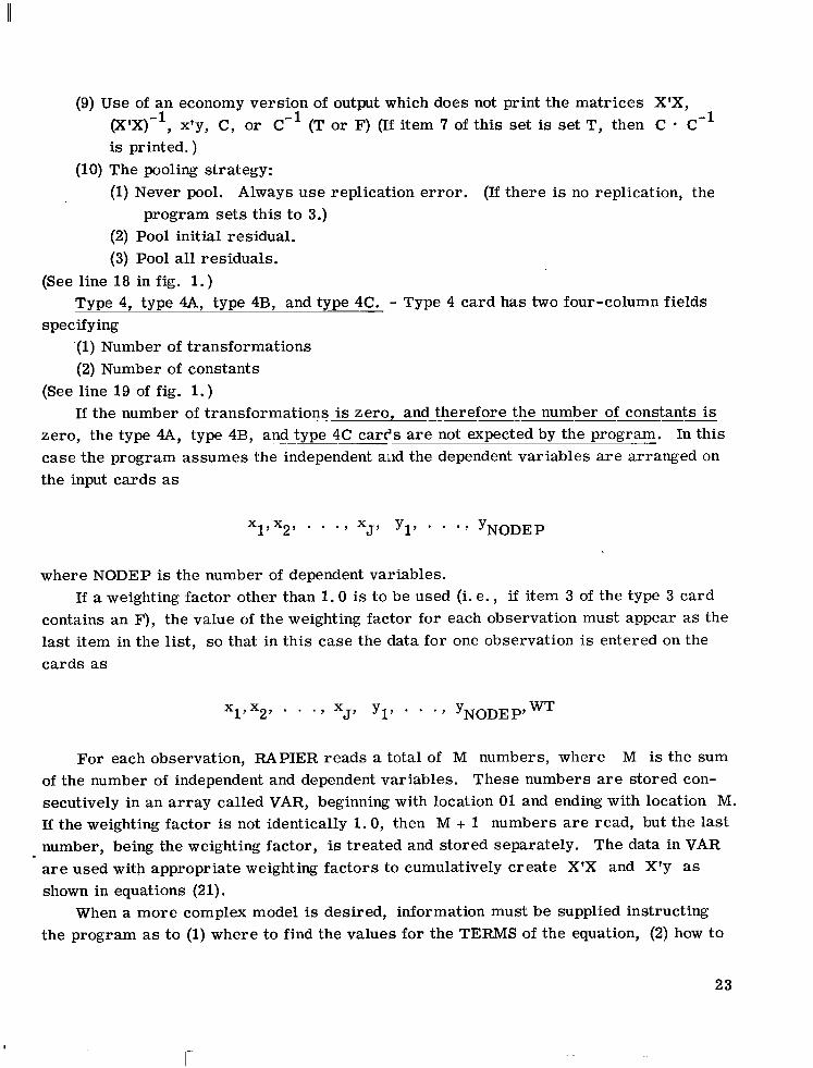
(See line 18 in fig. 1 . ) Type 4, type 4A, type 4B, and type 4C.

specif ying '(1) Number of transformations (2) Number of constants

(See line 19 of fig. 1 . )

- Type 4 card has two four-column fields

If the number of transformations is zero, and therefore the number of constants is . .

~ ~ _ ~ _ _zero, the type 4A,type ~ 4B, and type 4C cares a r e not expected by the_ program. In this case the program assumes the independent and the dependent variables a r e arranged on the input cards as

where NODEP is the number of dependent variables. If a weighting factor other than 1 . 0 is to be used (i. e . , if item 3 of the type 3 card

contains an F), the value of the weighting factor for each observation must appear as the last item in the list, so that in this case the data for one observation is entered on the cards as

For each observation, RAPIER reads a total of M numbers, where M is the sum of the number of independent and dependent variables. These numbers are stored consecutively in an a r ray called VAR, beginning with location 01 and ending with location M. If the weighting factor is not identically 1 . 0 , then M + 1 numbers a r e read, but the last number, being the weighting factor, is treated and stored separately. The data in VAR are used with appropriate weighting factors to cumulatively create X'X and X'y as shown in equations (21).

When a more complex model is desired, information must be supplied instructing the program as to (1) where to find the values for the TERMS of the equation, (2) how to

23

I

I I l l

create the TERMS from the variables and constants, and (3) what the values are for the constant terms. This can be achieved easily by use of the type 4A(TERMS), type 4B(TFUNSFORMATIONS), and type 4C(CONSTANTS) control cards (see p. 29). These three types and their functions can best be described by considering the sample model given by equation (27) as an example which illustrates their application.

An ar ray called CON has a twofold purpose. First, if the number of constants designated in the second field of the type 4 card is nonzero, that number of constants will be read from the type 4C card and stored consecutively in this a r ray beginning with location 01. If the number of constants is zero, the type 4C card is not expected by the program. Second, all the intermediate and final results of transformations are also stored in the CON ar ray as the program obeys the instructions of the type 4B cards. The type 4A card must identify the relative location in the CON ar ray where the value for each TERM is to be found for constructing the X'X and X'y matrices.

The VAR and CON a r rays for this example are illustrated in figure 2. Five numbers are read for each observation: xl, x2, x3, yl, and y2. These numbers automatically enter the VAR ar ray beginning with location 01. Using transformation codes packed in fields of eight columns each on the type 4B cards, the program stores the result of each transformation into the appropriate relative location in the CON ar ray as designated by

Location VAR Location CON

04 05 Input constants 06 Input followed by terms

' for regression

61 62 63 64 65 66 Data stored are 67 * stored in same

relative location i n both arraysii y;;

97 -97 98 -9a 99 -99 J

Figure 2. - Map of VAR and CON arrays. Data transferred into any location of CON array beyond location 60are immediatelyduplicated in same relative location in VAR array.

24

the last two digits of the field. Each transformation code is made up of four subfields of two card columns each, with the following interpretation:

1 Operand VI 2 Operation OP Arithmetic operation 3 Operator CI Relative location in CON 4 Result CS Relative location in CON

Thus, subfield 1 always references the VAR ar ray and subfields 3 and 4 reference the CON array. The result of every transformation is a te rm which is stored in the designated location of the CON array, with the added feature that if the te rm is stored in relative location 61 or beyond, it is also stored in the VAR array. This is illustrated by the arrows in figure 2. This feature allows successive transformations to be performed more easily. The OP (operation codes) are tabulated in table In.

TABLE ID. - OPERATIONS~AND CODE NUMBERS _.

Operation Resulting operation )peration Resulting operation code code (OW (OP)

00 No operation 16 l.O/SQRT (VAR) 01 VAR + CONST 17 CONST**VAR 02 VAR*CONST 18 10. O*TAR 03 CONST/VAR 19 SINH(VAR) 04 EXP(VAR) 20 COSH(VAR) 05 VAR**CONST 21 (l.O-COS(VAR))/2. 0 06 A LOG(VAR) 22 ATAN(VAR) 07 A LOGlO(VAR) 23 ATAN2(VAR/CONST 08 SIN(VAR) 24 VAR**2 09 COS(VAR) 25 VAR**3 10 SIN(lr*CONST TAR) 26 ARCSIN(SQRT (VAR)) 11 COS(lr *CONST*vAR) 27 2.O%*vAR 12 l.O/VAR 28 1.0/(2.0%”rrAR) 13 EXP(CONST/VAR) 29 ERF(VAR) 14 EXP(CONST/VAR**2: 30 GAMMA(VAR) 15 SQRT(VAR)

’All function names and operations are consistent with FORTRAN N mathematical subroutines.

25

TABLE IV. - SEQUENCE O F TRANSFORMATIONS ~

rransformation VI OF C1 CS Interpretation number

01 01 02 02 03 03

00 00 00 00 00 00

00 00 00 00 00 00

11 61 12 62 13 63

x1 - CON(11) x1 -VAR(61), CON(61) x2 - CON(12) x2 - VAR(62), CON(62) x3 - CON(13) x3 - VAR(63), CON(63)

-61 02 61 17 x: CON(17)

8 62 02 62 18 x2 - CON(18)2

9 10

63 61

02 02

63 62

19 14

x i - cON(19) x1x2 - CON(14)-11

12 61 62

02 02

63 63

15 16

x1x3 CON(15) x2x3 - CON(16)-13

14 04 05

00 00

00 DO

20 2 1

y1 CON(20) y2 - CON(21)

-~--- _ _ . .__-

Table lV shows the sequence of transformations used to construct the te rms of the example in equation (27). (See lines 21 and 22 of fig. 1. )

The ar rays VAR and CON are shown in figure 3 both before and after one set of transformations performed on an observation. Note that CON now contains xl, x2, x3,

2 2 2x1x2, x1x3, x2x3, x l , x2, x3, yl, y2 along with unused locations. It may be that not all of these quantities are needed to express the model equation. The type 4A(TERMS) card must be used to supply the locations of CON which contain the te rms of the model equation. (Note that this allows the user to somewhat arbitrarily assign te rms to locations in CON.) The t e rms identifying the independent variables must be first, and the t e rms identifying the dependent variables last, just as in the assumed convention when no transformations a r e performed. Thus, in this case the te rms needed are , according to equation (27),

11 12 13 1 4 15 16 17 18 19 20 21

(See line 20 of fig. 1 . ) After the set of transformations has been performed on an observation, the contents

of the relative locations of the CON array specified on the te rms card a r e transferred

26

01

02

03

04 05

06

07

08

09

10

11

12

13

14

15

16

17

18

19

20

21

22

Location VAR CON

x 1

I x2 -X3

y1

y2

Bd a (b) Afler transformations. (c) Afler terms

selection.

Figure 3. - Arrays VAR and CON before and after transformations and terms selection, for the first example.

27

back to VAR in consecutive locations beginning with location 01. Thus, for this example, after selection of proper terms, the VAR a r ray contains

in consecutive locations as required by equation (27) and the convention on independent and dependent variables. The bo te rm is accounted for by setting the proper item of type 3 input to T.

There are three important facts to note concerning types &, 4B, and 4C. First, the transformation with OP = 00 is an identity transformation which simply transfers data from VAR to CON. If transformations are desired at all, a minimum requirement is that all variables at least be moved to CON so that the selection of t e rms will have a number to move back to VAR. Second, constants used in the transformations are stored in CON in locations beginning with 01 in sequence. Suppose there are NC constants initially supplied. Then if-a transformation has any of the locations 01 through NC refer-~ _ _

enced in subfield 4, a te rm will replace the constant. Third, the use of TRANSFOR~

MATIONS and TERMS overrides the convention that independent variables must precede dependent variables on the input data cards. The convention holds t rue for the t e rms card data in this case.

The sequence of input and formats is as follows: (1) Type &(TERMS): One o r more cards, as necessary, with two-column fields

denoting the relative locations of the CON ar ray containing the final t e rms to be used in regression model (Up to 60 independent and nine dependent t e rms may be supplied. See line 20 of fig. 1.)

(2) Type 4B(TRANSFORMATIONS): A s many cards as necessary, with 10 transformations per card, each transformation being composed of four two-column subfields (A maximum of 100 transformations may be performed. See lines 21 and 22 of fig. 1.)

(3) Type 4C(CONSTANTS): As many cards as necessary, containing the required number of constants in (5E15.7) format. A s many as 60 constants may be supplied.

A second example is shown to illustrate the flexibility afforded by the TERMS, TRANSFORMATIONS, and CONSTANTS. Consider a model with two independent and two dependent variables with four t e rms given by

2 2 + b x x 3 kbo + b l X 1 + b x 3 1 2 + b4X1 = y1 = y2

28

where k = 1 .0 . Then a sequence of transformations which could be used is

cs Interpretation

01 00 00 61

01 02 61 62

61 02 62 63 01 00 00 14 02 00 00 02 02 02 61 12 03 00 00 11

04 12 01 09

The TERMS information should then be

x1 x2

14 02

~

XI - CON(61), VAR(61)

x: - CON(62), VAR(62)

X; - CON(63), VAR(631 x1 - CON(14) x2 - CON(O2) x1x2 - CON(12) yl - CON(11)

k- CON(O9) Y2

3 k x1x2 x1 y1

y2

12 6 3 11 09

The total process is illustrated by figure 4 and the type 4 input given in figure 5. Type 5. - In type 5 input, one card with one one-column field and one three-column

field specifies (1)U s e of t-statistics to reject insignificant t e rms (T or F) (2) Probability level that t-statistic must meet to be considered significant (This is

written without a decimal point; e. g., 95-percent significance level is supplied as 950, 99.9 percent as 999, etc. See line 23 of f ig . 1 . )

Type 6. - In type 6 input, one card with one one-column field specifies that the data contain replicated points (T or F). If there a r e replicated data points, as many cards as are needed a r e read, containing 20 four-column fields specifying

(1) The number of replicate sets (2) The number of replicates in each replicate set

Note that it is not safe for the program to assume that all data points with the same levels of the independent variables are t rue replicates. For this reason, the user must arrange replicate sets. RAPIER does check that all independent t e rms are the same within a replicate set. If not, the program stops. A nonreplicated data point is considered to be a group of size 1. Note that the data in table I are grouped to clearly indicate the repli

29

01

02

03

04

05

06

07

08

09

10

11

12

13

14

15

Location VAR

63

64

(a) Before transformations. (b) After t ransformat ions. (c) Af ter t e rms selection.

Figure 4. - Arrays VAR and CON before and after t ransformat ions and te rms selection, f o r t h e second example.

30

FORTRAN STATEMENT

Figure 5. - Sample input form for type 4 Input

cated data points. There a r e 1 4 such groups. Thus, the first field of the second type 6 card contains a 14, and the remaining fields contain the count of the replicates in each group. (See lines 24 and 25 of fig. 1.)

Type 7. - In type 7 input, one card with one two-column field specifies the input unit number the data will be on. The remainder of the card is used to supply the format in which the data will be supplied. Note that if a weighting factor other than 1 .0 is to be used, it will be read with each data point, and the format must allow for this. The current example uses a weighting factor of l. 0.

The format is (5F6.0) since there a r e three independent variables (xl, x2,x3) and two dependent variables (yl, y2). If a weighting factor other than 1 .0 is used, it must appear with every data point, and the format could, for example, be (5F6.0, F10.3). (See line 26 of fig. 1.)

Type 8. - Type 8 input consists of the input variables. Each observation consisting of the given x's and y's is read by execution of one READ statement. Thus, there will be at least one card for each observation. If the transformation option is not used, the program expects the first variables read to be the independent variables and the last ones to be the dependent variables; that is, the data must be arranged as

31

Otherwise, if transformations are used, appropriate use of the te rms card information allows for more flexibility of input. (See lines 27 to 50 of fig. 1.)

Type 9. - In type 9 input, one card with one column is used t o indicate if predictions are desired (T o r F). (See line 51 of fig. 1.) If this is false, a new case is started. If it is true, the following cards are read: One card with one four-column field specifies the number of predictions desired. This is followed by cards with the values of the independent variables at which predictions are desired. Only the final regression model is used, but the number of independent and dependent variables originally supplied on the type 2 data cards are read. All transformations in type 4 input are performed. Then the proper t e rms are chosen by the program to correspond to the final model. The dependent variables are not needed and, hence, may be left off the data card unless one of the transformations of the dependent variables might lead to an impossible operation (e. g., log(y2)). (See lines 52 and 53 of fig. 1.)

32

SAMPLE OUTPUT

SAHPLE R A P I E R PROBLEH HOOEL EQUATION I = 1.2

Y I I l = 80 + B l * X l +nz*xz * 8 3 + X 3 + B l Z * X l * X Z + 8 1 3 * X l + X 3 + 8 2 3 + X Z * X 3 + B l l + X l + * 2 + B Z Z b X L + t Z + 8 3 3 b X 3 b * Z ERR

X 1 = TEHP b. X 2 = T I H E *+ DATA COOED TO STANOARIZEO U N I T X 3 = PRESS +* v i = POUNDS o u r P u T V Z = COST OF OPERATION

THE DATA I S FROH A N INCOHPLETE FACTORIAL DESIGN Y I T H OHE R E P L I C A T I O N I F I C T I T I O U S DATA1

3 2 9 2 5 TTTTFFFFF2 THERE IS A 80 TO ESTIHATE NTERHIK 1-

1 1 12 13 14 15 16 17 i n 1 9 20 2 1 THE TRAYSFJRMATIONS ARE

I O 0 1 1 I O 0 6 1 2 0 0 1 2 2 0 0 6 2 3 0 0 1 3 3 0 0 6 3 61 2 61 17 62 2 6 2 18 63 Z 6 3 19 61 2 6 2 1 4

6 1 2 6 3 15 62 2 63 16 4 0 0 2 0 5 0 0 2 1

I 5 F 6 - 0 1 SAHPLE RAPIER PROBLEH

OBSERVED VARIA3LES. YEIGHT = 1.000000 -1.000000 -1.000000 -1.000000

OBSERVAl lON = , 9.170330 38.50300

1

TERHS O F THE E2UATION. OBSERVATION = 1 - 1.000000 -1.000000 -1.000000 1.030333 L.003300 1.000000 1. ooaooo 1.003000 1.033335 9.170000 38.50000

t t REPLICATE SET 1 b++bb++.bl.b+b+b*blbbb+bbbbb*bbb+*+bbbbbb++b++b+bbbbb+bbbbb*bbbbbbbbbbbbbb*bb*b;**bbbb+bbb+bbbbbb+bb ~ + * + b b b b b + ~ b b t D b l l ~ l ~ b ~ ~ ~ ~ b ~ b b b + ~ + ~ ~ + ~ b b ~ b b b b b b * ~ + ~ b b b ~ b b b + b b + b b b b b b b b b b * b * b b b b b b b * b b b b b b b b b b ~ ~ b ~ ~ ; b ~ b ~ ; ; b b b b b ~ b b b b b $ b ; b b + b b b

OBSERVED VAR IAJLES, Y E I G H T = 1.000000 1.000000 - 1.000000 -1.000000

OBSERVATION = , 12.76330 43.10300

2

TERMS OF THE EaUATlON, OBSERVATION = Z 1.000000 -1.000000 -1.000000 -1.00D530 -1.003300 1,000000 I . 000000 1.000000 1 . 3 3 1 3 3 3 12.76000 43.10000

OBSERVED VARIA3LES. YEIGHT = 1.000000 1.000000 -1.000000 -1.000000

OBSERVATION = , 12.97333 44 .OO 3 0 0

3

TERHS O F THE E lUATION. OBSERVATION = 3 1- 000000 - 1.000000 -1.000000 -1.335 3 3 3 -1.0033 00 1.000000 1.000000 1.003000 1.33>>31 12.97000 44.00000

at REPLICATE SET 2 b ~ b l b + + + + * b b b b b b b b l t + b * + b b b ~ + b b b b + b b b b b b b ~ b b b b + b b b b b b b b * b + * b b b b b b b ; * ; b ~ + b b ~ ~ b b ~ b b : ; b b ~ b ~ * b b b b b b * + + * b O E P . YAa. 1 SSO= 0.2204895E-01 Sun= 25.733000 MEAN= 12.865000 OEP .VAR . 2 S S Q = 0 . 4 0 5 0 5 9 8 SUM= 87 .099999 MEAN- 43.550000

t + + l b l b b b b b b + ~ ~ + l ~ ; ~ b b ~ ~ b b ~ B + ~ ~ b b b b b + + b b b b b b + b b ~ b b b b * * + b b b ~ b b b b * b b b b b ~ b * * b b b b b b b * b b b b b b b b b b b b ~ b ~ ; b b B ~ b ~ b ~ ; b b b ~ b b ~ b b b * b b b * * * b b

OBSERVEO VARIA3LES. NEIGH1 = 1.000000 OBSERVAT I O N = . - 1.000000 1.000000 -1.000000 9.1 10300 58,30300 TERHS OF THE EQUATION. OBSERVATION = 4

-1.000000 1.000000 -1.000000 -1.0333JO 1.000300 - 1.000000 1.000000 I . aooooo 1 .333333 9.110000 58.30000

OBSERVED VARIABLES. Y E I G H T = 1.000000 -1.000000 1.000000 - 1.000000

OBSERVATION = ,8 . 9 5 3 3 3 3 58 .70JOO

TERHS OF THE EQUATION, OBSERVATION = -1.000000 1.000000 -1.000000

5 - 1 . 3 9 3 3 3 3 1.000300 - 1.000000 1.000000 1.000000 1 . 3 3 ) ) J )

n. 960000 56.70000

OBSERVEO VARIABLES. WEIGHT = 1.000000 OBSERVATION = . 6 1.000000 1.000000 -1.000000 17.030JO 6 3 . 2 0 3 0 0

1ERHS OF THE EQUATIONt OBSERVATION 5

1.000000 1.000000 -1.000000 6

I .0033 3 3 -1.003100 - 1-000000 1.000000 1.000000 1 . 0 3 3 3 ) ) 17.03000 63.20000

33

.... . .

** REPLICATE SET 4 * ~ * ~ * t ~ l $ $ ~ ~ i * t $ ~ ~ ~ * * I . * * ~ ~ * ~ ~ * * * ~ $ ~ $ ; ~ ; $ ~ ~ * ~ * * ~ ~ ~ ~ ~ ~ ~ ~ * * $ ~ ~ ~ ~ ~ ~ ~ ~ $ ~ $ ~ ~ $ ; ~ ~ ~ ~ ~ ; ; ~ ; ~ ~ ~ ~ ~ ; ~ ~ ~ ~ ; ~ ~ ~ ; ; ; ~ ; ~ **ft**********@~ * ~ * * * * l ~ b ~ i ~ ~ ~ * * ~ l t ~ * * * ~ ~ * * * ~ * ~ ~ * ~ ~ ~ * * ~ * ~ ~ ; $ ; ; + $ $ ~ * * * * $ $ $ $ ~ ~ $ ~ * ~ * ~ ~ $ ~ $ $ ~ ~ ~ ; $ $ b ;b~$$b;$;;;$;b;Ct~$;C~~$$;~$$~~

OBSERVED VAR IABLESI WEIGHT = 1.000000 OBSERVATION = , 7 -1.000000 -1.000000 1. 000000 9 .053330 38 .70300

TERMS O F THE EOUATION, OBSERVATION = 7 -L.000000 - 1.000000 1.000000 1.030330 -1.003100 -1.000000 1.000000 1 .000003 1 .333333

9.0 5000 0 3 ~ 7 0 0 0 0

OBSERVEO VARIA3LES. UEIGHT = 1.000000 OBSERVATION = 8 -1.000000 - 1.000000 1.000000 8.853333 39 .60300

TEKMS JF THE EQUATION. OBSERVATION = 8 - 1.000000 -1.000000 1.000000 1.030353 -1.003300 - 1.000000 1.000000 1.005003 1 .033331 8.860000 39.60000

L$ REPLICATE SET 5 **t*t*$$~tltt*+t~$~**$*$*$*$;~****$;;*~**~***+*$~*****~*~~**~*~**~b**~;$$$~b$**~$*~$$;***$***;*$$;;$ OEP. VA4. 1 SSP= 0.L805115E-01 SUM= 17.913003 MEAY- 8 .9549999 OEP. VAR . 2 SSP= 0.4050293 SUM= 7 e . 2 9 9 9 ~ MEAN= 39.150000

$ $ * $ $ ~ $ l ~ * ~ l $ * * * t C ~ ~ ~ $ $ ; ; $ ; $ $ * * * $ ; $ ~ ; $ * ~ $ * $ ~ * $ ; * $ * * $ ~ * ~ * ~ ~ ~ ~ ~ $ ; ~ $ ~ * * $ $ * ~ $ * ~ $ * ~ * ~ ~ ~ * ~ * ~ * ~ $ ~ ~ ~ * b ; b ; ; ; * ; * * b ; ; $ ~ ~ ~ ; * ~ $ $ ~ $ * * ~ ~ ~ ; ; $

UBSERVEO V A R I A ~ L E S I WEIGHT = 1.000000 OBSERVATION = , 9 1.000000 - 1.000000 1.000000 12.63330 44. LO300

T E k M S 3F THE E?UATION. OBSERVATION = 9 1.000000 -1 .000000 1.000000 -1.030333 1.003300 -1.000000 1.000000 1. onoooo 1 . 0 3 3 3 3 1 1 2 - 6 0 0 0 0 44- 10000

OBSERVED V I R IABLES, WEIGHT = 1.000000 OBSERVATION = , LO 1.000000 -L.000000 1.oooooo 13.21330 4 3 . 8 3 3 0 0

TERMS O F THE E4UATION1 OBSERVATION = LO i.aoooo0 -i.oaaooo 1.000000 -1.003 3 J 3 1.D03300 -1.000000 1.000000 1 .000033 1 .331311 13.21000 4 3 . eoooo

I+REPLICATE SET 6 $ttt$$$tl4tCli*+$*l***************$*;*$*~**~******$~~***~**~~~~~*b***bb$$$$$***~~***$*~****$~*~~$*$* OEP. VAR. I SSP= 0 .1860542 SUM= 25 .813303 MEAY= 12 .905000 OEP. VAR. 2 ssa= 0 . 4 5 0 1 ~ , 3 ~ - 0 i SLIM= ~ 7 . 9 0 3 0 0 0 MEAN= 43 .950000

I $ $ $ $ + ~ ~ ; ~ ~ $ t ~ ; l ~ t ~ $ $ ; $ ; ; $ ; $ b ~ $ $ $ ~ ~ l t t l ~ ~ ~ ~ ~ ~ $ $ ~ ~ ~ ~ ~ $ ~ $ ~ $ $ ; ; $ $ ~ ~ ~ ~ $ $ ~ ~ ~ $ $ ~ $ ~ $ $ ~ ~ ~ ~ ~ ~ ~ $ $ $ ~ * ~ b * b ~ $ $ $ ; ~ $ ~ b b ~ $ $ ~ ~ ~ ~ ~ ; $ ~ $ $ $ ~ ~ ~ ~ $ ~

OBSERVED VAKI13LESn WEIGHT = 1.000000 0BSERVATION = . I 1 I . 000000 1.000000 I . 000000 17.20333 62 .10300

TERMS 3F THE EaUATION. OBSERVAr IUN = 11 1.000000 1.000000 1.000000 1.000130 1.003300 1.000000 1.000000 1.003000 1 . 3 3 1 3 3 3 17.2000 0 62 .10000

OB5ERVEO VARlAdLES. W I G H T = 1.000000 OBSERVATION = 1 2 1* 0 00000 1.000000 1.000000 17.34333 62.83JOO

TERMS J F THE E>UATION. OBSERVATION = 1 2 1.0w000 I . 0 00 00 0 I . 000000 1.033333 1.000300 1.000000 1.000000 1.003003 L.331311 17.04000 62 .80000

OBSERVED VARIABLES, WEIGHT = 1.000000 OBSERVAT I O N = , 13 0 0 0 9 . b 1 0 3 3 3 49.10300

TERMS OF THE EQUATIONt OBSERVATION = 1 3 0 0 0 0 0 0 9.610000 49.10000

OBSERVED VARIA3LES. WEIGHT = 1.000000 OBSERVATION = , 1 4 0 0 0 1 0 . 0 l J 3 3 49 .30300

I E W S J F THE EaUATION, OBSERVATION = 1 4 0 0 0 0 0 0 10. O l O O O 49.30000

OBSERVEO VARIABLES, WEIGH1 = 1.000000 OBSERVATION = 15 0 0 0 10.12130 50.10300

TERMS 3F THE EQUATION. OBSERVATION = 15 0 0 0 0 0 0 0 10.12000 50.lOOOO

OBSERVED VAR IASLES, WEIGHT = 1.000000 OBSERVATION = I 16 0 0 0 9.953130 5 I . eo300

TERnS O F THE EPUAI ION, OBSERVATION = 1 6 0 0 0 0 3 0 0 9.950000 51.80000

OBSERVED VARIABLES. WEIGHT = 1. 000000 OB5ERVATION = I 17 -2.000000 0 0 11.78330 50.10300

TERMS O F THE E?UATION, OBSERVATION = 17 -2.000000 0 0 -0 -0 0 4.000000 0 0

11.78000 50.10000

OBSERVED VARIABLES, WEIGHT = 1.000000 OBSERVATION = , 18 2.000000 0 0 23.83350 57.60300

TEFMS J F THE EOUATLON, OBSERVATION = 18 2.000000 0 0 0 5 0 4. ooowo 0 3 2 3 .E3000 5 7 - 60000

34

OBSERVED VARIABLES. WEIGHT = 1.000000 2.000000 0 0

OBSERVATION = ,22.90330 58.10300

19

TERMS OF THE EIIUATION, OBSERVATION = 19 2 .oooooo 0 0 0 0 0 4.000000 0 3 22.90000 58.10000

OBSERVEO VARIA3LES, WEl;HT = 1.000000 OBSERVATION = I 20 0 -2.000000 0 7.993330 28.60000

TERMS OF THE EQUATION, OBSERVATION = 20 0 -2.000000 0 -0 0 -0 0 4.000000 0 7.990000 2n. 60000

OBSERVED VARIABLES, UEIGHT = L.000000 OBSERVATION = , 21 0 2.000000 0 12.11333 7 1 .00300

TERMS OF THE E Q U A T I U N ~OBSERVATION = 21 0 2.000000 0 0 0 0 0 4 . 0 0 3 300 0 12.11000 71.00000

r = 1.00oooo OBSERVATION = ,73.20300

22

n 0 0 0 0 0 4.000000 0

OBSERVE0 VARIABLES. WEIGHT = 1.000000 0 0 -2.000000

OBSERVATION = ,l O . l I l 3 3 48.70300

23

TERMS 3F THE E2UATION. OBSERVATION = 23 0 0 -2.000000 0 -0 -0 0 0 $.111311 10.l1000 48.70000

OBSERVED V I R I A 8 L t S . HEIGHT = l.000000 0 0 -2.000000

OBSERVATION = ,10.01333 49.90300

24

TERMS OF THE EJUATION, OBSERVATION = 24 0 0 -2.000000 0 -0 - 0 0 0 $ . 0 3 1 1 1 3 10.01000 49.90000

OBSERVEO VARIABLES. W E I G I T = l.UOOOO0 OBSERVATION = , 25 0 0 2.00u000 10.02330 50.80300

TERMS JF THE EPUATION. OBSERVATION = 25 0 0 2.000000 0 0 0 0 0 4.031103 10.02000 50.00000

SUMS J F IYDEP AN0 U t P VAHIABLES 4.0000000 0 -2 .0000000 0 2.0000300 -2 .ooooooo 24.000000 2 c . 003300 24 .000000 308.10000 12n2.2000

X TRANSPOSE X MATHIX ROW 1 L4.00000 *OW 2 0 24.00000 ROW 3 2.000000 -2.000000 24.03330 ROW 4 -2.000000 2.000000 4.000000 12.03000 ROW ROW

5 6

0 4.000000

4.000000 0

2.300113 -2.003113

-2.001000 2.003000

12 .ooooo 0 12.00000

ROW HOW ROW

7 8 9

10.00000 2.000000 2.000000

-2.000000 6.000000

-2.000000

0 0

-8 .000339

3 3 3

2.000000 2.000000 2.000000

-2.000000 -2.000000 -2.000000

50.03030 12.03000 12.01330

53.03133 12.03333

ROW 9 60.00000

X TRANSPOSE Y Y A T R I X ROW I 127.5600 260.5000 ROW 2 22.36000 23 8.5000 R O U 3 -12.24000 -110.3000 ROW 4 8.740000 12.90000 ROW 5 26.62000 13 9.7000 ROW 6 -9.680000 -95. Y O 0 0 0 .... ROW 7 382.0000 1260. LOO ROW 8 275.1600 1276.100 KOU 9 268.5200 1194.500 HEbNS OF IYUEP AND O t P VARIABLES

0.1600000 0 -0.8000000E-01 0 3.0003000E-01 -0.8000000E-01 0.9600000 0.9503333 0-9600000 12.324000 51.288000

35

X TRANSPOSE X M A T R I X WHERE X I S D E V I A T I O N FROM MEAN ROY 1 23.36000 ROY 2 -0 24.00000 ROY 3 2.320000 -2.000000 23.84030 ROY 4 -2.000000 2.000000 4.000000 12.03000 ROY 5 -0.320000 4.000000 2.160313 -2 .003000 11.84000 ROY 6 4.320000 0 -2.160313 2.003000 0.160000 11.84000 ROY 1 6-160000 -2.000000 1.923313 -0 0 . 8 0 0 0 0 0 E - 0 1 - 0 . 8 O O O O O i - 0 1 36. 9 5 3 3 0 ROY 8 - 1 . 8 4 0 0 0 0 6.000000 1.920330 -3 0 - 8 0 0 0 0 0 E - 0 1 -0.BOOOOOE-0 1 -1 I . 04000ROY 9 -1.840000 -2.000000 -6.085J33 -3 0.80OOOOE-01 -0- 8003001-01 - 1 1 . 0 4 3 3 0

ROY 9 36-96000

X TRANSPOSE Y M A T R I X WHERE X AN0 Y ARE O E V l A T I O N S FROM MEAN ROY I 7 8 . 2 6 4 0 0 5 5.34 800 ROY 2 2 2 . 3 6 0 0 0 238.5000 ROY 3 12.40800 -7 .723999 ROY 4 8.740000 1 2 . 9 0 0 0 0 ROY 5 1.972000 3 7 . 1 2 4 0 0 ROY 6 14.96800 6 . 6 7 6 0 0 0 ROY 1 86.22400 ZY. 18800 ROY 8 -20.61600 4 5 . 1 8 8 0 0 ROY 9 - 2 7 . 2 5 6 0 0 - 3 6 - 41 2 00

CORRELATION COE FF I C I E NT S ROY 1 1.000000 ROY 2 -0 I . 000000 ROY ROY

3 4

0 . 9 8 3 1 0 2 � - 0 1 - 0 . 1 1 9 4 5 5

-0. 8 3 6 1 2 5 E - 0 1 0 .117851

i.oJoj,3 0.236432 1 .003000

ROY 5 - 0 - 1 9 2 4 1 4 E - 0 1 0 .237289 0 .128565 - 3 . ~ 6 7 7 a 9 1.000000 ROY 6 0.259760 0 -0.128566 3 . 1 6 7 7 8 9 0 . 1 3 5 1 35E- 0 I 1 000000 ROY 7 0.209642 -0 .671 5 1 9 E - O l 0.6 46 8 I 8 E-0 1 -0 0 - 3 8 2 4 2 7 E - 0 2 -0 .382427E-02 I . 003350 ROY 8 - 0 - 6 2 6 2 0 3 E - 0 1 0 .201456 0 - 6 4 6 0 1 8 E - 0 1 -3 0 . 3 8 2 4 2 7 E - 0 2 -0 .382427E-02 - 0 . 2 7 8 7 3 1 ROY 9 -0 .626203E-01 -0 .671519E-01 -0.2348 2 6 -0 0 - 3 8 2 4 2 7 E - 0 2 - 0 - 3 8 2 4 2 7 E - 0 2 - 0 . ? 3 8 7 3 1

3 5 . 9 5 3 1 1 -1 1 . 3 4 3 1 3

1 . 1 1 1 1 1 3 -3 .298751

ROY 9 1.000000

SAMPLE RAP IW PROBLEM EACH G L U M N - C O V r A l N S THE C J E F F I C I E N T S CONSTANT T E R M 160)

9.97 3 9 9 5 50.151 2 3 REGRESSION C O E F F I C I E N T S IB1...-.8K1

2.9403 7 4 2.031365 0,98737 7 10 .16832

-0 .138332E-01 0 .370808 1 .068721 -0 .467807 0 .820396E-01 -0 .397416 0 .203767E-01 -0- 1 9 1 4 8 1 E - 0 1 1.90943 7 0 .965708 0.9 1034 E- 0 2 - 0.571 182E -01 0.3 302 73E- 01 -0 .596032E-03

FOR ONE DEPENDENT TERM

ANOVA OF REGRESSION ON DEPENDENT VARIABLE I U***U*****t+*. . . . . . . . . . . . . . . . . . . . . . . . . . . . . . . . . . . . . . . . . . . . . . . . . . . . . . . . . . . . . . . .

SOURCE SUMS OF SPUAHES DEGREES OF FREEDOM MEAN SPJARES

R E G R E S S I W 4 2 5 . 3 9 0 3 6 9 9 4 7 . 2 6 5 5 9 6 4 RES IOUAL 1.08622742 15 0 . 7 2 4 1 5 1 6 0 E - 0 1

TOTAL 426.476597 24 . . . . . . . . . . . . . . . . . . . . . . . . . . . . . . . . . . . . . . . . . . . . . . . . . . . . . . . . . . . . . . . . . . . . . . . . . . . . . R SPUAREO = SS?LREGI / S S P I T O T I = 0 .997453 R = . 9 9 8 7 2 6 STANDARD ERRDP O F E S T I M A T E 0 . 2 6 9 1 0 1

U S I N G POOLING STR4TEGY 2 THE ERROR MEAN SUUARE = 0 . 7 2 4 1 5 I b E - 3 1 WITH DEGREES OF FREEDOM = 1 5 F=MSIREGl /MSIERRI= 6 5 2 . 7 0 COMPARE TO F l 9 . 1 5 1

ANOVA OF LACK OF F I T ~ * * * ~ * * * * * U * * * * ~ * * + * * C * * * * * * C * * * * * * * * * * * * * * * * * * * * * * * * * * * * * * * * * * * * * * * * * * * * * * *

SOURCE SUMS J F SQUARES DEGREES OF FREEDOM MEAN SPJARES

LACK OF F I T 0 . 1 6 9 4 5 2 6 7 5 0 . 3 3 8 9 0 5 3 3 E - 0 1 REPL I C A T IOU 0.91677475 13 0 . 9 1 6 7 7 4 7 5 E - 0 1 RES IOUAL 1.08622742 1 5 0 . 7 2 4 1 5 1 6 0 E - 0 1

F = I S l L O F l / M S t R E P S l = 0.370 *~~*H*~***~**~**********~*~~~*********.*************************************

36

--

N O V A J F REGRESSION ON JCPENOENT VARIABLE 2 *****9*~~b*9b**t*****b**b**bbb*bb*******bb****bbb**********b**b***b*******bb*

SOURCE SUMS OF SOUARES DEGREES OF FREEDOM MEAN SOJARES~~

REGRESSION 253 9.42480 3 2 8 2 . 1 5 8 3 1 0 RES I OUA L 10.4 015808 15 0 . 6 9 3 4 3 8 1 2

TOTAL 2 5 4 9 . 8 2 6 3 9 24 *.**~************b*******b**b**b***b*b***b****b***b**b*b********************b**

R SOUAREO = S S P I R E G I I S S O I T O T I = 0.995921 R = . 9 9 7 9 5 8 STANDARD ERROR OF ESTIMATE 0 . 8 3 2 1 3 0

U S I N G P J O L I N G S T R A T E G V 2 THE ERROR MEAN SOUARE = 3 . 6 9 3 4 3 8 7 Y l T H DEGREES OF FSEEODM = 15 F ~ M S l R E G l / Y S l E R ~ l ~406.90 COMPARE TO F I 9. 1 5 1

A M V A OF LACK OF F I T *.**+t+*****#~tb**.****b*b**b***b*b**********b***b***********bb***************

S3URC E SUMS OF SOUARES DEGREES OF FREEDOM MEAN SPJARES

LACK OF F I T 3 .52811 7 0 4 5 0 . 1 0 5 1 4 3 4 0 REPLICATION 6 . 8 1 2 8 6 3 1 1 13 ‘ 3 . 6 8 7 2 8 6 3 8 RES IOUAL 10.401 5808 15 0.69343872

F = M S I L O F I / M S I R E P S I = 1.021 *~b***t~*~~t#b~*~*t~****bb*b***bb*b************b*b***b*****b*b*b******bbbb****

SUMS OF SOUIRES DUE TO EACH VARIABLE I F I T YERE LAST T O ENTER REGRESSION 1 i b 4 . 5 5 a 7 78.54016 2 19.45477 2063.286 3 0 - 3 4 9 9 7 2 E - 0 2 2 .514691 4 10.44572 2.001442 5 0 . 6 6 5 3 6 7 E - 0 1 1.561362 6 0.405068E-02 0 . 3 5 7 6 9 l E - 0 2 7 %.39906 24 .65779 8 0.221086E- C 2 0.870364E-01 9 0 - 2 6 8 2 9 9 E - 0 1 0 .938933E-05

STANDARD O E V I A T I J Y OF RESRESSION COEFFICIENTS IDERIVEO FROH DIAGONAL E-EqENTS OF I X TSANSPOST X I I Y V E 7 S E M A T R I X I 0 0 . 1 2 8 4 3 9 0.397453 1 0.616818E-01 0.190874 2 0 .602399E- 01 0.186412 3 0 - 6 2 9 2 4 6 E - 01 0.194120 4 0 . 8 8 9 8 3 6 E - 0 1 0 .275359 5 0 . 8 5 5 8 7 o E - 0 1 0 .264848 b 0 . 8 6 1 5 5 6 E - 0 1 0.266608 7 0 . 5 2 3 3 4 0 E - 0 1 0 .161947 8 0.521002E-01 0.161224 9 0 - 5 2 3 4 4 O E - 0 1 0 .161978

I X TRANSPOSE X I INVERSE M A T R I X non I 0 . 5 ~ 5 3 9 3 ~ - 0 1 R O Y 2 -0 .514411E-02 0.5011 I l E - 0 1 ROY 3 -0 .116754E-01 0 .115598E-01 0 . 5 4 6 7 1 9 E - 0 1 ROW 4 0 . 1 9 l l Z Z E - 0 1 -0 .179948E-01 - 0 . 2 8 5 5 2 l E - 0 1 0 . 1 0 9 3 4 3 R O Y 5 0 .892031E-02 - 0 . 2 2 2 9 1 2 E - 0 1 - 0 . 1 9 3 4 3 4 E - 3 1 0 . 3 0 1 3 6 Z E - 0 1 0.101155 R O Y 6 - 0 . 2 4 1 1 8 7 E - 0 1 0. 130194E-02 0 . 1 9 3 8 1 9 E - 0 1 - 0 . 3 1 1 0 8 l E - 0 1 - 0 - 1 3 3 6 4 4 E - 0 1 0 . 1 0 2 5 0 3 R O Y 7 -0 .892995E-02 0 .149314E-02 0 . 1 9 8 ’ + 4 3 E - 0 2 - 3 . 3 5 5 1 8 5 E - 0 2 - 0 . 2 2 3 8 l l E - 0 2 0 . 4 1 1 1 0 4 E - 0 2 0 . 3 1 9 ? l ’ + E - O 1 ROY 8 0 . 6 8 3 9 5 5 E - 0 3 - 0 . 1 1 1 6 1 7 E - 0 2 - 0 . 1 8 8 3 l O E - 3 2 3 .262bbbE-02 0 . 2 9 6 3 8 0 E - 0 2 - 0 . 6 1 9 1 3 4 E - 0 3 3 . 1 5 2 5 0 9 E - 0 1 0 . 3 1 ’ + 9 1 3 E - 3 1 ROY 9 -0 .21193OE-02 0 .256242E-02 0 .915151E-02 - J . 5 1 3 1 2 1 E - 0 2 -0 .397529E-02 0 . 3 8 2 7 5 8 E - 0 2 0 . 1 5 8 3 3 5 E - 0 1 0 .1535OZE-31

R O Y 9 0 . 3 7 8 3 5 4 - 0 1 SAMPLE R A P I M PROBLEM

CALCULATED T S T A T I S T I C S THE 1 S T A T I S l I C S C4N BE USED TO T E S T THE NET REGRESSION COEFFICIENTS 81 1 1 .

41.6100 b LO. 6 4 2 4 6 16 - 3 9 0 1 3 54 .54160 0 .219838 1.904315 12 .01031 1 .698899 0.958553 1.50054 1 0.2365 10 0.118214E-01 36 -4856 1 5.963113 0.174729 0 .354280 0 .630967 0 .367971E-02

UNOER NULL HVPJTHESIS THE INTERVAL I - T . T I WHERE 1 I S GIVEN ABOVE. HAS APPROX P R 3 8 A B I L I T V L I S T E J BELOW. MINUS S I C S I INDICATES PROB EXCEEDS -999 .

1 -0.999 -0.999 2 -0.999 -0 .999 3 0.171 0.924 4 - 0 . 9 9 9 0.890 5 0.647 0.845 6 0.184 0.056 r -0.999 -0.999 8 0.135 0.211 9 0.463 0.002

THE OESIRED VALUE OF PROBABIL ITY IS 95.0 PERCENT . THE TERM X I 8 1 I S BEING DELETE0

THE NUYBER OF DEPENDENT VA3IABLES YAS 2 I T I S B E I N G SET T O ONE AN0 THE REJECTION OPTION E X E 3 t l S E 3 OY 3EPENJZNT VARIABLE I

37

CORRELATION COEFFICIENTS R O Y 1 1.000000 ROW 2 -0 1.000000 ROU 3 0.983102E-01 - 0 - 8 3 6 1 2 5 E - 0 1 1.000330 R O Y 4 - 0 . 1 1 9 ~ 5 5 0. i I 7~5.1 0.23 6 4 9 2 I .00~000 ROW 5 -0.192414E-01 0.237280~. ~~~ ~~.~ -0. IL77hP0 . 1 2 8 5 6 6 .. .. .- . I .nnnooo.... . ROY 6 0.259760 0 -0.128555 3 . 1 6 7 7 8 9 0 - 1 3 5 1 3 5 E - 0 1 1 . 0 0 0 0 0 0 ROY 7 0.209642 - 0 . 6 7 1 5 1 9 E - 3 1 0 . 5 4 6 8 1 8 E - 0 1 -0 0 . 3 8 2 4 2 7 ~ - 02 - 0 . 3 8 2 4 2 7 ~ - 0 2 I . no0310 ROY 8 - 0 . 6 2 6 2 0 3 E - 0 1 - 0 . 6 7 1 5 1 9 E - 0 1 -0.234825 -3 0.3 824 2 7E- 0 2 - 0.3 82 4 2 7 f - 0 2 -0.2 98 73 1

SAMPLE RAP IW PROBLEM EACH COLUMN CONTAINS THE COEFFICIENTS FOR ON6 DEPENDENT TERM CUNSTANT TERM 180)

9.989932 REGRESSION COEFFICIENTS lBl.....EKI

I 2.940208

6 0 - 2 0 5 2 7 2 E - 0 1 7 1.905733 9 0 . 2 9 3 7 2 2 E - 0 1

ANOVA OF REGRESSION ON DEPENDENT VARIABLE 1 8***88*8888**8******88*88****8**8*****8*8***88**88***88**8E88*8888**8E*******8E

SUURC E SUMS OF SQUARtS DEGREES OF FREEDOM MEAN S?JARES

R EGR� SS ION 4 2 5 . 3 8 8 1 6 5 8 5 3 . 1 7 3 5 2 0 6 R E S I O U I L 1 . 0 8 8 4 3 2 3 1 16 0 . 6 8 0 2 7 0 2 3 E - 0 1

TOTAL 4 2 6.4 7 6 5 9 7 2 4 * 8 8 ~ 8 b ~ 8 8 b 8 8 U b b l t b + 8 ~ ~ 8 ~ ~ 8 8 8 ~ ~ 8 k 8 ~ 8 8 ~ 8 ~ 8 ~ ~ 8 8 8 8 8 ~ 4 $ ~ 8 8 ~ * ~ E ~ ~ E ~ ~ ~ ~ ~ ~ E ~ ~ 8 E * ~ ~ ~ ~ 8 E

R S3UAREO = S S a I R E S I / S S i l l T O T l = 0 . 9 9 7 4 4 8 R = . 9 1 8 7 2 3 STAUOIRD ERRUd OF ESTIMATE 0.260820

U S I N G POOLING S T R A T E G Y 2 THE ERKOR MEAN SJUAHE = 0 . 7 2 4 1 5 1 b E - 3 1 Y l T H DEGHEES OF FREEDOM = 1 5 F = M S I H E G l / M S I E R K ) = 734.29 COMPARE T O F l 8. 1 5 1

ANOVA OF LACK OF F I T * 8 * 8 8 * 8 8 8 * * * 8 8 * * * * * * * 8 * * * * * ~ 8 * 8 ~ * * * 8 8 8 8 * * 8 * * * * * * * * * * * * * * ~ * * * ~ * * * 8 * * * * ~ * * ~ * * * ~ 8 *

SOURCE SUMS OF SQUARES OEGREtS OF FREEOUH MEAN SQUARES_-___-__________-_______________________--------------------------------------LACK OF F I T 0. I 7 1 6 5 7 5 6 5 0 . 2 8 6 0 9 5 9 3 E - 0 1 REPL ICATIUN 0 . 9 1 6 7 7 4 7 5 13 0 . 9 1 6 7 7 4 7 5 E - 0 1 RES IOUAL I . 0 8 8 4 3 2 3 I 15 0 . 6 8 0 2 7 0 2 O E - 0 1

F = M S l L O F l / M S l R t P S l = 0.312 *************8*.*.**8*88***888888*8*8*****888888*888*888888888*88****8*8*888***

SUMS 3~ S ~ U A R E SDUE TU E A C ~VARIABLE IF I T WERE L A S T To E N T E R REGHESSI[IV I 1 6 4 . 5 7 9 2 2 20.16795 3 0 - 3 2 7 7 2 5 E - 0 2 4 10.45084 5 0 - 6 5 5 2 6 l E - 0 1 6 0.41 I I I C E - 0 2 7 114.8713 9 0 . 2 7 1 3 5 7 E - 0 1

STANDARD D E Y I A T I J V OF RESHESSLUN COEFFICIENTS I O E R I V E O FROM OIAGONAL E-EYENTS 3 F I X TRANSPUS: X l I Y V f Q S E M I T Q I X 1 0 . 9 0 4 j o 1E- 01 0.6 1 6 7 4 5E- 01 0.5’) 27 7 % - 0 1 0.6 2 8 6 9 $E- 0 1 0.889087E-01 0.854878E-01 0.86 15 1 ?E- 0 1 0.47848 BE- 01 0.4798 2 3E- 01

I X TRANSPOSE X I INVERSE MATRIX KUU I 0 . 5 2 5 L 6 * - 0 1 R O Y 2 -0 .500332E-02 0 - 4 8 5 2 3 4 E - 0 1 R O Y 3 -0.116409E-01 0. l l i ? I L E - O l 0 . j 4 5 8 2 3 E-) I ROM 4 0 . 1 9 0 6 4 3 E - 0 1 - 0 . 1 7 4 5 4 1 E - 0 1 -0.2 8 42 3%E -0 I 3 . 1 3 3 159 ROW 5 0.886623E-02 - 0 - 2 1 6 8 1 1 E - 0 1 -0. I 9 1-34 1 E -01 0.335 2 8 5 E - 0 1 0 . 1 0 0 9 2 0 ROW 6 - 0 . 2 * 7 0 7 4 E - 0 1 0 . 7 1 7 4 3 7 E - 0 2 0.19352 7E-0 1 - 0 . 3 1 3 6 5 3 E - 0 1 - 0 . 1 3 3 1 5 4 E - 0 1 0 . 1 0 2 4 9 3 ROW 7 -0.92082ZC-02 0 . 4 b 3 2 5 5 E - 0 1 0.2 7 52 5 3 E -02 - 0 . 4 6 2 6 5 3 E - 0 2 - 0 . 3 4 4 3 9 6 E - 0 2 0.496919E-02 0 . 3 1 5 1 5 t E - 3 1 ROU 8 - 0 . 2 3 9 3 9 1 5 - 0 2 0.566052E-02 0 . 3 9 0 > 5 3 E - 3 2 -D.618589E-02 - 0.5 I 6 5 28E- 0 2 0 . 4 0 7 6 4 l i - 02 (1.97 07 I 5 F - 3? 3 . 3 I 7 > 1 1E- l I

38

SAMPLE RAPIER PROBLEM

CALCULATED r s r A T I s r I c s THE 1 S T A T I S T I C S C4N BE USEJ TO TESr THE NET REGRESSION COEFFICIENTS 8111.

4 7 - 6 1 303 16.68845 0.212736 12.01326 0 .951245 0.238269 3’4.82824 0.6 12 1 4 7

UNDER NULL HYPJTHESIS THE INTERVAL I - T I T I WHERE T IS GIVEN ABOVE. HAS APP;(OX P R 3 B A B l L I T Y L I S T � ) BELOU. MINUS SIGN I N O I C A I E S PRO8 EXCEEDS -999

1 -0.Y99 2 -0.999 3 C.165 4 -0.999 5 0.644 6 0.185 7 -0 .999 9 0.451

THE OESIREO VALUE OF PROBABIL ITY IS 95.0 PERCENT THE TERM X I 3 1 IS BEING DELETE0

CORRELAT I O N COE FF I C LENTS ROW I 1.000000

.. ~~~~~~

ROW 3 - 0 . 1 1 9 4 5 5 o. 1 I 7 8 5 1 1.003J33 ROW 4 -0 .192414E-01 0 . 2 3 7 2 8 4 -0 .167739 1.033000 ROW 5 0 . 2 5 9 7 6 0 0 0 .167739 0.135 1 3 S E - 0 1 1.000000 ROW 6 0 .209642 -0 .671519E-01 -0 0 .382427E-02 -0 .38242 7E- 0 2 I.000000 ROW 7 -0 .626203E-01 -0 .671519E-01 -0 0 .382427E-02 -0 .382427E-02 - 0 . 2 9 8 7 0 1 l.OOJJ30

Rnu 7 - n 1.000000

SAMPLE RAPIER PROBLEM EACH COLUMN CONTAINS THE CON5TWT TERM 1801

9 .989235 REGRESSION COEFFIC IENTS

I 2 .931356 2 0 .991988 4 1.061119 5 0 .766166E-01 6 O.25268EE-01 7 1 .906408 9 0 .318004E-01

COEFFIC IENTS FOH ONE DEPENDENT T E R M

I B L . . . . .BKl

TOTAL 426.4 7 6 5 9 7 2 4 . . . . . . . . . . . . . . . . . . . . . . . . . . . . . . . . . . . . . . . . . . . . . . . . . . . . . . . . . . . . . . . . . . . . . . . . . . . . . . R S1UAREO = S S a I R E S l f SSdlTOTl = 0.99744D R = .9Y8719 STAYOARO ERROR OF ESTIMATE 0 .253413

USING POOLING STRATEGY 2 THE ERROR MEAN SQUARE = 0 . 7 2 4 1 5 l b E - 0 1 W I T H DEGREES OF FREEOOM = 15 F = M S I R E G l / N S I E R R I = 839.18 COMPARE T O F I 7. 1 5 )

ANOVA OF LACK OF F I T ...............................................................................

SOURCE SUMS JF SQUARES DEGREES OF FREEOOM ME4N SOJARES

LACK OF F I T 0.1 7 4 9 3 0 5 7 7 0 . 2 4 9 9 0 0 8 2 E - 0 1 REPLICATIOH 0 .91677475 LO 0 .91677475E-01 RESIOUAL 1 .09170532 1 7 3 . 6 4 2 1 7 9 6 0 E - 0 1

F = M S I L O F l f M S I R E P S I = 0.2 73 . . . . . . . . . . . . . . . . . . . . . . . . . . . . . . . . . . . . . . . . . . . . . . . . . . . . . . . . . . . . . . . . . . . . . . . . . . . . . . .

SUMS OF S3UARES DUE TJ EACH VARIASLE I F I T WERE LAST T O ENTER R E G R E S S I 3 Y I 172.4090 2 21 .28251 4 11 .93265 5 0 .623348E-01 6 0.667668E-02 7 115.4596 9 0 .337156E-01

39

STANDARD O E V I A T I J N OF R E X E S S I f f l COEFFICIENTS I O E R I V E O FROU DIAGONAL E-E'IENTS 3F I X TSANSPOSi XI INVERSE MATRIX 1 0 0 - 9 0 3 7 0 8 E - 0 1 1 0 - 6 0 1 9 9 3 E - 0 1 2 0 . 5 7 8 6 4 2 E - 0 1 4 0.826629E-01 5 0.825796E-01 6 0.832182E-01 7 0.477436E-01 9 0 . 4 6 6 0 4 9 E - 0 1

I X TRANSPOSE X I INVERSE U A T R I X ROY I 0.500441E-01 ROY 2 -0 -ZbZO83E-02 0 - 4 6 2 3 7 0 E - 0 1 R O Y 3 0 . 1 3 0 0 3 ~ - 0 1 - 0 . 1 1 6 3 7 4 E - 0 1 0.9435OBE-01 ROY 4 0.477268E-02 -0- 1 7 7 5 2 7 E - 0 1 0 - 2 0 5 3 5 5 E - 0 1 0 . 9 4 1 7 0 7 E - 0 1 ROY 5 - 0 . 2 0 5 8 0 4 E - 0 1 0.32 1 3 9 7 E - 0 2 -0.20983 7 E - O I -2 .651 0 7 0 E - 0 2 0.9 5 6 3 2 9 E - 01 R O Y 6 -0 .862117E-02 0.406919E-02 - 0 - 3 1 9 3 2 8 E - 0 2 - 0 . 2 4 7 6 0 0 E - 0 2 0 . 3 9 9 3 3 2 E - 0 2 0 . 3 1 4 7 7 6 E - 0 1 ROY 7 - 0 . 2 8 0 4 7 5 6 - 0 3 0- 3 6 3 2 3 8 E - 0 2 -0.132611E-02 - 0 . 1 6 3 0 5 5 E - 0 2 0 . 5 6 3 2 4 9 E - 0 3 0 . 9 2 0 7 4 0 5 - 0 2 3 . 2 9 3 9 b O E - 3 1

SAMPLE RAP IW PROBLEU

CALCULATEO r s r A r i s r i c s THE T S T A r l S I l C S T 4 N BE USE3 TO TEST THE NET REGRESSION COEFFICIENTS 8111.

48.79386 17.14339 1 2 . 8 3 6 7 1 0.927792~~

0 - 3 0 3 6 4 5 39.93009 0.682340

UNDER NULL HYPOTHESIS THE I N T E R V A L 1 - T . T ) YHERE T I S G I V E N ABOVE. HAS APPROX P R O B A B l L l T Y L I S T E J BELOW. U I N U S SlGU I N O I C L T E S PROS EXCEEDS -999.

1 -0.999 2 -0.999 4 -0 .999 5 0.632 6 C.233 7 -0.999 9 0.495

THE D E S l l E O VALUE OF P R O a A B l L I r Y I S 95.0 PERCENI THE TERM X I 6 1 IS E E I N S DELETE0

CORR ELATION COE FF I C I E N T S R O Y 1 1.000000 ROY 2 -0 1.000000 R O Y 3 - 0 . 1 1 9 4 5 5 0.11 7 8 5 1 I . 0 3 3 J 1 3 ROU 4 - 0 . 1 9 2 4 1 4 E - 0 1 0 . 2 3 7 2 8 9 - 0 . 1 6 7 7 8 9 1.031000 R O Y 5 0.209642 - 0 . 6 7 1 5 1 9 E - 0 1 -0 0 . 3 8 2 4 2 7 E - 9 2 1.000000 R O Y 6 - 0 . 6 2 6 2 0 3 E - 0 1 - 0 . 6 7 1 5 1 9 E - 0 1 -0 3 . 3 8 2 4 2 7 E - 0 2 - 0 . 2 9 8 7 0 1 I . 000000

SAMPLE RAPIER PROBLEM EACH UILUUY C O U r A l H S THE C O E F F I C I E N T S FOK ONE DEPENDENT TERU CONSTAUT TERU 1801

9.907362 REGRESSION COEFFICIENTS 181 9.. . B K I

I 2.942794 2 0 . 9 9 1 1 3 9 4 1.066665 5 0.783369E-01 7 1.905353 9 0 . 3 1 6 5 1 6 E - 0 1

ANOVA OF REGRESSION ON DEPENDENT VARIABLE 1 **U*******************t***********************************************~*******

SJURCE SUUS JF SUUAKES DEGREES OF FREEOOH MEAN S3UARES

~~

TOTAL 4 2 6 . 4 7 6 5 9 7 2 4 . . . . . . . . . . . . . . . . . . . . . . . . . . . . . . . . . . . . . . . . . . . . . . . . . . . . . . . . . . . . . . . . . . . . . . . . . . . . . . . R S7UARED = S S J I R i S I / S S O I T O T I = 0 . 9 9 7 4 2 5 K = . 9 9 0 7 1 1 STAYOARD ERROR OF ESTIUATE 0.247024

U S I N G P J O L I N G STRATEGY 2 THE ERROR UEAN SOUARE = 9.7241516E-01 Y I r H DEGREES OF FREEO3rl = I5 F=US(REGl/MS(ERRJ= 979.03 COUPARE TO F l 6 . 1 5 1

40

m u

ANUVA OF LACK OF F I T . . . . . . . . . . . . . . . . . . . . . . . . . . . . . . . . . . . . . . . . . . . . . . . . . . . . . . . . . . . . . . . . . . . . . . . . . . . . . . . S3URCE SUMS 3 F SUUARES OtGKEES OF FREEOUM MEAN SJJAHES

LACK OF F I T 0.18160248 B 0 .22700313E-01 REPL ICAT IUY 0. '916 7 1 4 7 5 1) 0.9 I 6 7 7 4 7 5 E-01 R E S l O U I L 1 .09837723 1 3 0. h l U 2 0 9 5 7 E - 0 1

SUMS 3 F SJUARES DUE T O EACH VARl AtlLE I F I T YERE L A S I T O ENTER REGRESSIOY 1. .189.8499 i 21 .29583 4 12.67660 5 0.65473t.E- 01 7 115.Y460 9 0-33404s-01

SIANOARU D E V l A T 1 3 N OF REGLESSION C U E f F l C l E N T S I O E N l V E O FROM DIAGONAL ELEMENTS OF I X T3ANSPUSE X I I N V E 3 S S MATRIX I 0 0 - 9 0 1 6 0 0 E - 0 1 1 0 - 5 7 4 7 3 7 E - 0 1 2 0.57796%-01 4 0 .806197E-01 5 0 - 8 2 3 8 5 O E - 0 1 7 0 .476170E-01 9 0 .466024E-01

I X TRANSPOSE X I INVERSE MATRIX HOW 1 0.456152E-01 - . 2 - O . I V ~ V I A F - O ~- 0 . 4 6 1 7 9 n ~ - n i... - . I . .... ..

&Ob 3 0.848598E-02 -0.109320E-01 &OW 4 0.337156E-02 -0.17533gE-01 R O k 5 -0 .776179E-02 0.393498E-02 ROW 6 -0.1592bZE-03 0 .361345E-02

SAMPLE HAP LER PROdLEM

C .950 864 40.01411 0.679185

UNOtH NULL HVPJTHESIS THE INTERVAL I - 1 . T ) MINUS S lGY INDICATES PRO8 EXCEEDS .99V.

1 -0.999 z -0 .999 4 -0.999 5 C.643 7 -0.999 9 c.493

T H t OtSLRED VALUE OF P R O d A B l L l l V 1 5 95.0 THE TERM X i 91 I S BEING DELETED

CONRELATION COEFFIC IENTS ROW I 1.000000 HOW 2 - 0 1.000000 R O Y 3 - 0 . 1 1 9 4 5 5 o . i i 7 t l 5 i R O Y 4 -0.192414i-01 0.231289 ROU 5 0 . 2 0 9 6 4 2 -0.611519E-01

SAMPLE RAPIER PROBLEM EACH COLUMY CONTAINS THE COEFFIC IENTS FOR CONSTAYT TERM (801

10.02689 REGRESSI3N COEFFIC IENTS i B 1 n... . 8 K I

1 2.942962 2 0.987325 4 1.0676LB 5 0 .80070LE-01 7 1.895660

0.d97537E-01 O.191055E-01 J .937275E-01

-0.231532E-02 -0 .223413E-02 0 . 3 1 3 1 0 9 E - 0 1 -0.902437E-33 -3 .16422LE-02 0 .918388E-02 0 .299907E-01

W E R E T I S G I V E N ABOVE. HAS APPROX P R O B A t l I L I l V L I S T E I BELOW.

PERCENT

1.0003~0 -0.167739 1.003000 -0 0 .382427E-02 1.000000

ONE DEPENDENT TERM

I

41

REGRESS ION 425.344822 5 8 5 . 0 6 8 9 6 4 0 RESIDUAL 1 . 1 3 1 7 7 4 9 0 1i 0 . 5 9 5 b 7 1 0 3 E - 0 1

TOTAL 4 2 6 . 4 1 6 5 9 7 2 4 * * * * * * . * * * * . * * * * * * * * * * * * * * 4 * * * 4 * 4 * * * * * * * * * * * * * * * * * 8 * * * * 4 * * * * * * * * * * * * * * * * * * * 8 * * 4

R SIUAREO = SSUIREGI / SSJITOTI = 0.997345 K = , 9 9 8 6 7 2 STANDARD ERROR OF ESTIMATE 0.244051

U S I N G P 0 3 L I N G STR4TEGY 2 TdE EKROK MEAN SUUARE E 3 . 7 2 O l 5 1 6 E - O l Y l T H DEGREES OF FQEEO3'4 = 15 F - M S l R E G I / M S t E R R I = 174.74 COMPARE TO F I 5 . 1 5 1

LACK OF F I T 0.Z1500015 P 3 . 2 3 8 8 8 9 0 b E - 0 1 R E P L I C A T I O N 0 . 9 1 6 7 1 4 1 5 10 0.9 167 1 4 1 5 E-01 RES I O U I L 1.131 7 7 4 9 0 13 0.5956 7 103 E-01

SUMS 3 F SJUASES 3UE TO EAZH VARIABLE I F I T YERE LAST TO ENTER REGRESSIJV I 1 8 9 . 8 7 5 1 2 21.33362 4 12.703ia 5 0.68468SE- 01 1 126.0952

STANOARO O E V I A T I J N OF R E i K E S S I O N COEFFICIENTS I O E R I V E O FROM DIAGONAL E-E'IENTS 3 F I X TRANSPOSE XI INVERSE MATRIX 0 0.688638E-01 I 0.574732E-01 2 0 . 5 7 5 2 3 2 E - 0 1 4 0.806076E-01 s 0 . 8 2 3 4 5 5 ~ - 01 7 0 . 4 5 4 2 8 2 E - 0 1

I X TRANSPOSE X I INVERSE M A T K l X R O Y 1 0 . 4 5 6 1 4 3 E - 0 1 R O Y 2 - 0 . 1 9 0 9 9 % - 0 2 ROY 3 0 . 8 4 8 1 1 9 i - 0 2 ROb 4 0 . 3 3 6 2 8 4 E - 0 2 ROY 5 -0 .771302E-02

SAMPLE RAPIER PRJBLEM

CALCULAIEO T S T A T I S T I C S THE I S T A T I S T I C S L 4 N BE USED

51 -2058 1 17.16396 13.24464 0.912368 4 1- 7 2 8 6 8

0 . 4 5 6 9 3 b E - 0 1 - 0 - 1 0 8 2 3 3 E - 0 1 -0-1 7 3 3 6 0 E - 0 1

0 . 2 8 2 8 4 6 f - D Z

TO T E S T THE

UNDER NULL HYP3THESIS THE I N T E R V A L I - T . 1 1 MINUS SIGY I N J I C A T E S PRO3 EXCEEUS -999 .

1 -0 .999 2 -0.999 4 - c . 9 9 9 5 0.654 7 -0.999

THE DESIREO VALUE OF P R O B A B I L I T Y I S 95.3

0 . 8 9 7 2 5 8 E - 0 1 O.193551E-31 3 . 9 3 5 3 7 5 E - 0 1

-0.204345E-02 - 0 . 1 7 3 1 2 5 E - 0 2 0 . 2 8 4 9 8 5 E - 0 1

NET REGRESSION C O E F F l C l E N l S 81 I I .

YHERE 1 I S G l J E N ABOVEt HAS APPROX P R J B A B I L I T Y L I S T E I RFLOW.

PERCENT THE TERM X I 51 I S B E I N G OELETEU

CORRELATION COEFFICIENTS ROU I 1.000000 ROW 2 -0 ROW 3 -0 .119+55 R O Y 4 0 . 2 0 9 6 4 2

SAMPLE RAPIER PROBLEM EACH COLUMN CONTAINS T H t CONSTAYT TERM I801

10.0 3236 REGRESSION C O E F F I C I E N T S

I 2.940086 2 1.002149 4 1.051323 1 1.897115

42

I . 000000 0-117 8 5 1 1.000330

-0.671 5 1 9 E - 0 1 -0 1.003000

C O E F F I C I E N T S FOR ONE OEPENOENT TERM

1 8 1 . . . . . B K I

1

- - - - - - - - - - - - - - - - - - - - - - - - - - - - - - - - - - - - - -

ANOVA U F REGIESSION ON J tPENDENT VARIABLE 1 ***.***1*******0*******+**8************b+*****b**************b*******0********b

SOURCE SUMS OF SUUARES DEGREES OF FREEUUU UEAN SaJAKES_-_-- - -- - - - - - - - -_- - .- --. . -- - - -_ _ - --_ _ --_ H E W E S S I O N 42 5.2 7 6 3 6 3 4 1 3 6 . 3 1 9 0 9 l RESIDUAL 1.2002 1 3 4 6 2 3 0 . b O O l l 6 7 2 E - O l

TOTAL 42 6.4 7 6 5 9 7 2 b *****OY*****+*********+0****b****b*********************************************

K S A U A R E D = S S J I R E S I ISsilIToTl = 0.9Y71n5 R = . 9 9 8 5 ~ 2 STANDARO ERROK OF ESTIUATE 0 .244973

U S I N G POOLIVG STIATEGY 2 THk ERROR MEAN S4UARE = 3 . 7 2 4 1 5 l b E - 0 1 d I T H DEGREES OF FREED3V = 15 F = M S l R t C l / ~ S l E K I l =468 .19 COMPARE T O F I 4. I 5 1

ANOVA OF LACK OF F I T *****t******++***************************+*****b*******************************

S3URC E SdMS OF SUUARES DEGREES OF FREEDOM

LACK OF F I T 0 .28345871 13 REPL ICAT 10'4 0.Y16774 75 13 K ES 1DUAL 1.2 0023 3 4 6 2 1

F = H S I L U F l l M S I ~ E P S I = 0.309************ *** *****+******b******C+*******************************************

MEAN SUJARES

3 . 2 8 3 4 5 8 7 l E - 0 1 0 .91677475E-01 0.6001 l 6 7 2 E - 0 1

SUUS 3 F S3UALES JUE TO EAZH VARIABLE I F I T MERE LAST T O ENTER REGRESSIJY 1 190 .0073 2 23.63953 4 17.H747b 7

STANDAHI) D E V I A l l U N OF HEGRESSION COEFFIC IENTS I U E R I V E D FROM DIAGONAL ELEYENTS OF I X TqANSPOSE X l I Y V F ? S F MATRIX I 0 0 . 6 8 6 3 3 7 6 - 0 1 1 0 .573971E-01 2 0 . 5 5 4 6 6 l E - 0 1 4 0 .788463E-01 7 0 .4540JbE-01

I X TRANSPOSE X I INVERSE MATRIX ROW 1 0 .454936E-01 R O Y 2 - o . I ~ ~ ~ ~ o E - o z0 . 4 ~ 4 8 4 1 ~ - 0 ~ HOW 3 0 .779683E-02 llil W 4 -0.765 l 9 2 E -02

SAMPLE WAP IER PROBLEM

CALCULATkU T S T A T I S T I C S THE T S T A T I S T I C S ,AN BE USED

51.22363 18.06778 1 3 . 3 3 3 8 2 41 .78336

-0. 729524E-02 0 .856487E-01 0.2 5 1 3 4 9 E-02 -0 I 4 9 4 2 4E-32 0.284 6 76E -0 1

TO TEST THE NET HEGRESSION CUEFFICIENTS 8 1 1 1 .

dNUkR VULL H W 3 T H t S I S TdE INTERVAL I - T - T I JHERE T I S G I V E N ABOVE. HAS APPROX P R 3 8 A 8 1 L I T Y L I S T E J 3ELOY. MINUS S I G N I N J I C A T E S PA38 E X C E k O S .9YY.

1 -c.v99 2 -0.999 4 -0 .999 1 -0.999

THE U E S l d t D YALUE OF P R O B A B I L I T Y I S 95.0 PERCENT SAMPLE RAPIEU PR30LEM

FOH tACH OkPENDENT TERM AND OBSERVATION I S PRINTED OBSERVED KESPONS� I Y OBSERVE01 CALCULATED KESPONSE I V CALCl RESIDUAL IYOt lS- YCALC=YDIF I STANUAHOIZEO RES13UAL 1 2 )

Y O B SER VE D 9.1700 Y CALC 9 .0386 Y OIF 0 .1314 5TUOENTILED 0 . 4 ~ 3 4

12 .760 12.816

-0.56UI3E-OI - 0 . 2 0 8 4

Y 08 S ERVEO 12.Y7O Y CALC 1 2 . ~ 1 6 Y D I F 0 .1539 STUDENT IZED 0 . 5 7 2 0

Y O 8 S t R V t U 9.1100 Y CALC 8.9402 V O I F 0.1698 STUDENTIZED 0.6310

Y 08SERVED 8.9600 Y CALC 8.9402 Y OIF O.1979E-01 S T U D � N l I Z E D 0.7354E-01

43

Y OBSkRVED Y CALL Y D I F STUOENTIZEO

Y OBSWVEO Y CALL Y D I F STUOENTIZED

Y OBSERVED Y CALL Y O I F STUOENTIZEO

Y OBSERVED Y CALL Y O I F STUDENT I Z EO

Y 0B S ER VE 0 Y CALL Y OLF S TUOENT I Z EO

Y OB SERVE 0 Y CALL Y O I F STUOENTIZEO

Y OBSERVED Y CALL Y O I F S TUOENT 12EO

11.030 16 .923 0 .1070 0 .3975

9 . 0 5 0 0 9 . 0 3 8 6 0 .1144E- 01 0.4252E-01

8.8600 9 - 0 3 8 6

-0 .1786 -0 .6635

12 .600 12-816

-0.2161 -0 - 8 0 3 0

1 3 . 2 1 0 12.1116 0 - 3 9 3 9 1 . 4 6 3 8

17.200 16 .923 0 . 2 7 7 0 1 . 0 2 9 2

1 7 . 0 4 0 16.923 0.1170 0 . 4 3 4 7

9 . 6 1 0 0 10.032

-0 .4224 -1 .5695

10.010 1 0 - 0 3 2

-0 .2236E-01 - 0 . 8 3 0 8 E - 0 1

10 .120 10 .032 0 . 8 7 6 4 E - 0 1 0 - 3 2 5 7

9 . 9 5 0 0 1 0 . 0 3 2

- O . B Z ~ ~ E - O I -0.3060

1 1 - 7 8 0 11.741 0 . 3 9 3 a E - 0 1 0 - 1 4 6 3

23 .830 23 .501 0 - 3 2 9 0 1 .2226

2 2 - 9 0 0 23 .501

Y OBSERVED Y CALC Y O I F STUOtNTILEO

Y OBSERVEO Y CALL Y D I F S TUOEN T I Z EO

Y 08SER YE 0 Y CALL Y D I F STUDENTIZEO

Y OBSWVEO Y CALC Y D I F STUDENTIZED

Y OBSERVED Y CALC Y O I F STUDENT IZED

Y OBSERVED Y CALC Y O I F S T U O E N T I Z E O

Y OBSERVED Y CALC Y D I F STUDENT IZED

Y OBSERVED Y CALC Y O I F STUDENTIZED

Y OBSERVED Y CALL Y O I F b TUOENT I ZED

Y OBSWVEU Y CALC Y O I F STUOENT 12 EO

Y OBSERVED Y CALC Y D I F STUDENTIZEO

Y OB S ER VE 0 Y CALL Y D I F STUDENTIZED

Y OBSERVED Y CALC V D I F SrUOENT [ZED

-0.6010 -2 .2333

7 .9900 8 .0281

-0.3806E-01 - 0 . 1 4 1 4

12 .110 12 .037 0 .7335E-01 0 . 2 7 2 6

11 .700 12.037

- 0 . 3 3 6 7 - 1 . 2 5 1 0

10.110 10.032 0.7764E-01 0 .2885

10.010 10.032

- 0 . 2 2 3 6 E - 0 1 -0. ~ ~ O U E - J I

I U - O Z D 10.032

- 0 . 1 2 3 6 E - 0 1 -0.$5 92E- 0 I

44

SAMPLE RAP I H 1 PKUBLEU

SKEWNESS ISHUULD B E NEAR Z E R U l

0.1928 KURTOSIS ISHUULJ B E NEAR THREE1

1.6949

CHl-SOUAKE IS Y O T COMPUTED FOR LESS THAN 30 OEGREES OF FREEOOU FOR ERROR.

FOR EACH SET OF INOEP VARIABLES THERE IS CUMPUTEO... PRED I L T E O R E SPIN SE VARIANCE OF K t C R E S S I O N L I N E STANDARD O E V l A T l O N OF NEGKESSION VARIANCE O F P K E o i c r E o VALUE STANOAUO D E V I A T I O N OF PREDICTED VALUE

I N P U l UATA FOR T H I S PREDICTED RESPONSE - 1.000000 1.000000 I.0i)0000 -0 -1

INUEPENUENT TEKHS ACCORDING TO F I N A L REGRESSION HOOEL- 1.000000 1.0u0000 -1.000000 1.000313

PRELjlCTEO KESPUNSE FUR ABOVE I N D E P VARIABLES 8.9402 1I 0.192847E- 01 0.138869 0.916998E-Cl 0.302820

Lewis Research Center, National Aeronautics and Space Administration,

Cleveland, Ohio, October 16, 1969, 129- 04.

45

APPENDIX A

PROGRAM DOCUMENTATION AND LISTINGS

The contents o is appendix include a flow chart of the program, a isting o t le routines used in RAPIER and their major functions, the call structure of the program, a dictionary of the program, and the listing.

General Mathematical and Logical Flow of Program

The flow of operation in RAPIER is illustrated in figure 6.

& transformations

replication errorC/-ICalculate

regressions

coefficients

Compute ANOVA data

+Compute

delete terms

minimum significance

critical level

Delete proper row and column from C

compute number of cells. compute chi-square! statistic

c3-7Given Xg

Compute

". XD GZP xo

Figure6 -Flowchartfor RAPIER

46

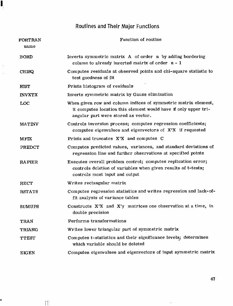
Routines and Their Major Functions

FORTRAN Function of routine name

BORD

CHISQ

HIST

INVXTX

LOC

MATINV

M F M

PREDCT

RAPIER

RECT

RSTATS

SUMUPS

TRAN

TRIANG

TTEST

EIGEN

Inverts symmetric matrix A of order n by adding bordering column to already inverted matrix of order n - 1

Computes residuals at observed points and chi-square statistic to test goodness of f i t

Prints histogram of residuals

Inverts symmetric matrix by Gauss elimination

When given row and column indices of symmetric matrix element, it computes location this element would have if only upper triangular part were stored as vector.

Controls inversion process; computes regression coefficients; computes eigenvalues and eigenvectors of X'X if requested

Prints and truncates X'X and computes C

Computes predicted values, variances, and standard deviations of regression line and further observations at specified points

Executes overall problem control; computes replication error ; controls deletion of variables when given results of t-tests; controls most input and output

Wri tes rectangular matrix

Computes regression statistics and writes regression and lack-off i t analysis of variance tables

Constructs X'X and X'y matrices one observation at a time, in double precision

Performs transformations

Wri tes lower triangular part of symmetric matrix

Computes t-statistics and their significance level!; determines which variable should be deleted

Computes eigenvalues and eigenvectors of input symmetric matrix

47

I11l1111lllilI I1 I I I I I I 1 1 1 1 I I I ,

Call Structure of Program

The call structure of the program is illustrated in figure 7.

j L O C

EIGEN

MATINV _I INVXTX

R STATS

SUMUPS TRIANG

Figure 7. - Cal l structure of RAPIER.

FORTRAN Mathematical name symbol

ACTDEV ei

ZEAN E@), P

B

BO

CHI X2

CON

com C

Dictiona ry of Program

Description

Error in observation i; difference between observed and predicted response

Expected or average value (of X)

Regression coefficients other than the constant

Constant regression coefficient

Chi- squared statistic

Constants used in transformations, and results of transformations

Correlation matrix

48


DELETE

ERFUVIS

EIG

FMT

FMTTRI

DENT

IDOUT

IFCHI

IFSSR

IFTT

IFWT

INPUT

INPUT5

INTER

IOUT

JCOL

KONNO

LENGTH

LIST

Description

Logical variable set to TRUE when deletion of te rms is desired

Estimate of cr2 used in hypothesis tests

Overflow area for storing part of modal matrix

Variable input format

Format for printing matrix

First identification printed at top of each page

Original sequence number of each term relating reduced models to original model

Logical variable set to TRUE if chi-square option is desired

Logical variable set to TRUE if sequential regressions are desired

Logical variable set to TRUE if t-statistics are desired

Logical variable set to TRUE if all weights of observations are 1 .0

Input logical tape unit number for data

Set equal to 5 to denote input device is card reader

Tape unit where input data is stored for chi-square qr prediction routines

Sequence number of term among those remaining which is to be deleted

Total number of independent and dependent te rms in regression model

Number of constants originally supplied for trans-format ions

Number of locations in correlation matrix storage area currently needed

Set equal to 6 to denote output device is printer

49


NARAY

NCON

NERROR

NODE P

NOOB N

BZERO

NOTERM J

NOVAR K

NPDEG NPDEG

NRES N - J - D

"TERM

NTRAN

NTRANS

NWHERE

NXCOD

P

POOLED SSQ(REP)

PREDCT

RE LSKW RE LSKW

50

Description

Number of replications per replicate set

Array containing addresses in CON array for use in transformations

Degrees of freedom for e r r o r mean square estimate

Number of dependent variables

Number of observations

Logical variable set to TRUE if constant bo coefficient should be in regression model

Number of te rms in current regression model

Number of independent variables to be read

Pooled degrees of freedom for replication e r ror

Degrees of freedom for estimation of residual variance

Array containing locations of te rms in CON array that should be in regression model

Array containing transformation codes for use in perform ing transformations

Number of transformations to perform

Location in X ar ray of first dependent variable; used in prediction routine to adjust for deleted te rms

Array containing addresses of variables (or te rms with address > 60) for use in transformations

Probability that the interval (-t,t) must have before a te rm is considered to be significant

Array containing pooled. sums of squares from replications for each dependent te rm

Logical variable set to TRUE if prediction option is desired

Skewness of distribution of residuals

FORTRAN name

RE LKUR

RE PS

RE PVAR

RESMS

RWT

s u m

sum2

SUMXX

SUMXXI

s u m

TOTWT

NLOF

NREG

NTOT

RNLOF

RNREG

Mathematical symbol

RELKUR

E X 2 , CY2

X'X

(xrx)-l

X'Y

C W i

Description

Kurtosis of distribution of residuals

Logical variable set to TRUE if there are replicate sets in the data

Array containing replication variance of each dependent term

Array containing residual mean square o r variance of each dependent te rm

Reciprocal of total weight

Array containing sums of independent and dependent t e rms

Array containing sum of squared independent and dependent te rms

Sums of squares and crossproducts matrix, and variance-covariance matrix of independent te rms

Variance-covariance matrix of estimated regression coefficients

Array containing sums of crossproducts of independent te rms with dependent terms

Sum of weight of observations

Before transformations a r e performed, this contains the variables as read in. After the transformations a r e performed, appropriate data from the CON array are placed here according to information on the te rms cards.

N - J - NPDEG - D Degrees of freedom for estimating variance due to lack of f i t

J Degrees of freedom for determining variance due to regression

N-D Total degrees of freedom

Reciprocal of degrees of freedom for lack of f i t

Reciprocal of degrees of freedom for regression

51

X


RNRES

STORY1

STORYC

STORYX

SATRTD

ECONMY

XCHK

S l E F T C B L C V

BLCCK O b T b C O P P C h l S M A L L I

X I F 1 1 9 X I S' IRbT, X NERRCR b X NOVbR. X P , X STORY I I

Description

Reciprocal of degrees of freedom for residual

Logical variable set to TRUE if product C - C- 1

is to be computed and printed

Logical variable set to TRUE if eigenvectors and eigenvalues of C are to be computed and printed

Logical variable set TRUE if eigenvectors and eigenvalues of X'X are to be computed and printed

Logical variable indicating that there are no degrees of freedom for residual if TRUE

Logical variable indicating suppress printout of x'x, x'x deviations, and C if TRUE

Array used in checking if a11 values of independent te rms are the same within a replicate set

Program Listing

B Y P A S S t B L E R O . O E L E T E , F I R S T . I F C H I , I F S S R . I F Y T . I N P U T , I N P U T S I I N T E R . J C O L t KONNO, LENGTH. L I S T . NOCEP t N O 0 8 v NOTERM. NPCEG. NRES. N T R A N S r N U H E R E V P R E O C T I R E P S , R h T ,

S I O R Y C . STORYX. T O T U T I YE IGHTt X E R R F X C . ECQNPY

L O G l C 8 L E C C h Y Y OCUeLE P R E C I S I O N R U T I T O T Y T , W E I G H T COCCCh l F R C T S l F C T ( 1 3 I ~ F M T T R 1 ( 1 4 1 DATb I N T E R / 3 / . I N P U T S / 5 / ~ L I S T l 6 l O A T 8 I F M T T R I ~ I ~ . I = l . 4 ~ / 6 H l 5 HR O , 6HW 1 5 . 2 , 6 H X . I B G I i 6H5-611 I ENC

52

S I B F T C RAPl IER

1 C T H I S I S R A P I E R p H A I V PROGRAM FOR R E G R E S S I C N A N A L Y S I S P R O V I D I N G 2 C I N T E R N A L E V A L U A T I O N QF RESULTS. 3 C * * * * * + * + * ~ * * * * * * * * * * + * * * * * * ~ * * * * t * * * * * * * * * * * * * * * * ~ * * * * * 4 * * * * * * * ~ * * * 4

5 C O P ~ ~ N / B f G / S U M X X ~ 1 8 3 ~ l ~ S U M X X I ~ l 8 3 O ~ ~ E I G ~ l 8 3 O l ~ S U M X Y ~ 6 O ~ 9 ~ ~ 6

X @ ( 6 C * 9) *CORR( 1 8 3 0 1 7 COCM@K/MED/ B O 1 9 1 v CON( 9 9 1 E R R M S ( 9 l r 8

X I C E N T t l 3 ) ) I D O U T ( 6 O ) * N C O N ( Z O O ) 4 9 X N T f R M l 6 O ) i N T R A N ( l O O 1 I N X C O O ( 1 O O ) r P O O L E D ( 9 l r 10 XREPVbR( 9 ) RE SM S ( 9 I ’* S U M X ( 1 3 8 ) r 11 X S U P X 2 ( 6 9 l r X ( $91, Z E A N t 6 9 1 SUMY2 ( 18 1 12

CCHlrCN /FRMiTS/ F M T ( L 3 l * F M T T R I ( l S l 13 COCCCN/SHALL / B Y P A S S ~ B Z E R O I D E L E T E I F ’ I R S T r I F G H I r I F S S R r 14

X I F T T r IFITTI I N P U T I N P U T S ) I N T E R r 15 X I S T R A T ) J C O L 9 KONNO L E N G T H @ L I S T * 16 X NERROR 1 N O b E P NOOB 9 N O T E R M i 17 X NOVAR NPlBEGs NRES 9 NTRANS. NWHERE v 18 X P I PREOCT 4 R E P S * R k T r 19 X STORY I STOR YC STORY XI TOTWT( WEIGHT9 20 X E R R F X C # ECONMY 2 1

LOG LCAL ECONMY 22 OOUBLE PREC IS I O N RWT 4TOTMT WE1GHT 23 LUG I C b L 8 Y P A S S I BZERO, D E L E T E e I F C H I * 24

X I F S S R t f F T T r IFWTI R E P S ( PRE DCT 9 25 X s T a R Y c , STORYXI STORY I9 F I R S T t E R R F X 0 2 6

L O G I C A L X S A V E 27 0 LP ENS ION XCHK ( 6 0 1 28 C O C C P N / C N T R S I I* IBCI I C r I C O L I 29

X I N E W r I NQCH Ior0 r IOUT 9 I R r 30 X I R C r I REP r I S l I T C , J V 3 1 X K * KBAR 32

C 33 C * * * * * * * * * # * * * * * * * , * * * * * * * ~ * * * t * * * * * * * * * * * * * * * * * * * * ~ * ~ * ~ * * * * * * * * * * * * * * * ~ * * 34 C 35

E Q U I V A L E N C E I N A R A Y r C 9 R R l i ( S c B O ) 4 ( S S Q r R E P V A R I 9 I Z C U 1 , S U M X X l 36 6)LCENS ION NARAY 1 1830 1 S ( 9I SSQ ( 9 1 37 O I C E h S I O N Z O U T i 11 38

C****+*r**~************+****+,**sr********~**~**~*********~******** 39 C ZERC OUT ALL D A T A ARRAYS EACH NEW DATA SET 40

L O O Y Z C U T = 9 4 7 0 41 DO Le1 J’lr I Z O U T 42

101 S U P X X 1 J I 9 O L O 43 44

c * * * * * * * * * ~ * * * ~ * * * k * * * * * * * ~ * * * * * * * * * * * * * * * * * * * # * * * * * ~ * * * * * * * * * * * * * * * * * k * 45 C REAC I O E N T I F f C A T I O N CARD A N 0 O P T l O N S C A R 0 46 C 47

R E A C l I N P U T 5 , 1 1 0 3 L r I D E N T 48 W R I T E ( L IST 111I I D E N T 49 F I RST=- TRUE. 50 ERRFXC‘.FALSE. 5 1

113 I F ( 1 ) 1 2 0 r 1 2 0 r l l 5 52 115 R E b C l I N P U T S * 3001 FMT 5 3

W R I T E t L 1 S T 1 3 0 1 ) FMT 54 a = 1-1 55

T C 113 56 120 REACJ I N P U T 5 r l 2 8 2 1 NOVAR,MOOEPrNOTERM6NOO5 57

W R I T E t L IST r 1283) NOVARr NODEP i N O T E R V r NOOB 58 REAC t I N P U T 5 9417) BZER(Bw.1 F T T r I F W T r f F C H 1 r STORYC r STORYX STORY Ir I F S S R 59

X PECONPY b I S T R A T 60 W R I T E ( L I S T r 1 3 8 1 BZERBcIFTTrIFWT~fFCHIISTCRYCISTORVXISTORYX~STORYI~I F S S R 61

X VECONMY L S T R A T 62 C 63

53

--- I I 1 I II 111111 I I I III I111 I 1 1 1 I I I I I 1111 1111.1111 I I,. .I

’ ’ I

C+*Y1**+++~+*8R**45**+****t*+**88*************$**~*************$*************** 64 C THESE ARE I N t T I A L I Z A T I O N S MADE BEFORE EACIH S E T OF D A T A 65 C ICOt C E T B R M f N E S THE N U M l E R O F V A R I A B L E S REAO PER O B S E R V A T I O N 66 C JCOL IS T H E NUMBER O F TERMS I N THE ‘TOTAL R E G R E S S I O N E C U A T I O N 67 C LENGTI- I S THE NUMBER O F STORES NEEDED FOR THE M A T R I C E S 68

tEh lGTI -= NOTERM*( N O T E R M + l I / 2 69 d C C L X h O V A R + NOOEP 70 JCOL 7 NQTERM +NODEP 7 1 NWPERE= NOTERM 72 REWIhC I N T E R 73 00 1 4 C J i l r Q O 74 ( I O C U T ( J 1 = J 75

140 N T E R C t J I ’ J 76 DO 1 4 5 J * l * l @ f f 77 NXCCC I J ) *J 78 NTR A h ( J 1 *O 79

145 N C C N L Z * J l = J 80 C 8 1 ~*+t******t***+*+$********~*******************$*~***************$*******82

I F ( B Z @ R O ) WRf T E I L I S T 4 1 9 0 1 83 I F ( . R C T . B Z E R C ) W . R I T E f L I S T r 1 7 0 ) 84

C****$**** t+**$*** t*******~**$~***$**~~*********$*********************** 85 R E 4 0 1 L N P U T 5 9 2 8 2 ) NTRANS,KONNO 86 iF(NTRANS.EQ;O) GO TO 255 87

2 2 0 REAO ( I N P C T 5 ~ 2 3 0 ) ( N ~ E R M ( K ) r K = l r O C O L ) 88 W R I T f ( L I S T r 2 3 5 ) ( N T E R M ( K l r K = l r J C O L ) 89

90REAC ~ I N P U T 5 r 2 3 U ~ ~ N X C O D ~ I ~ ~ N T R A N ( I ~ ~ N C O N ~ 2 * I ~ l ~ ~ N C ~ N ~ 2 * I ~ ~ I ~ l ~ N T R AANS J 91

92H R I T E ( L I S T * 2 4 O ) ~ N X C ~ D ~ I ~ r N T R A N ~ I ) ~ N C O N ~ 2 * I - l ~ ~ N C O N ( 2 ~ 1 ) ~ 1 ~ 1 ~ X h T R A N S )

I F ( K C N N O 9 2 5 5 r 2 5 5 r 2 5 G 250 R E A C ( I N P U T 6 ~ 2 6 O ) ( C 0 N ( I l r I = l ~ K O N N O )

W R I T E ( L I S T r 2 6 2 1 ( C O N L I ) r # = l r K O N N O ) ~ $ * * 9 * * * * * # * * * * * * * t $ * * * * ~ * ~ * 4 * * * * * * * * * ~ * * * * * * * * * * * * * * * * * * * * * * * * * * * * * * * * *

C 255 R E A C l L N P U T 5 r 2 5 7 1 O E L E T E r P

I F I C E L E T E I IFTT*.TRUE. C C***4****9d***********~*~*~********~$~*******$**9******$~*************** C l iF T t E R E ARE R E P L I C A T E D P O I N T S READ I N THE NUMBER O F P O I N T S AND C THE NUMBER O F R E P L I C A T I O N S , S I N G L E D A T A P O I N T S ARE OATA P O I N T S C R E P L I C A T E D ONCE. OBSERVED D A T A MUST B E ARRANGED I N THE ORDER C 1 P P L I E D HERE.

REAC4 I N P U T 5 9 2 5 7 ) R E P 3 X S A V f = . F A L S E I

265 IF( .KOT.REPS) GO TO 290 R E A C l I N P U T 5 * 2 8 2 ) IREP,(NARAY(I)rf=lrIREP) NPCEGqO d R E P t l I C = N L R A Y ( l ) KSAVE=.TRUE. DO 315 I * l r N Q D E P P O C L E O I I ) = C o o S ( I k f O . 0

315 SSC( f )=O:OC C * * 8 * * * * * $ t + * * t * * + * * * * * * ~ * # * * ~ * * * * * $ * * ~ * * ~ * * * * * * * * * * * * * * * * * * * $ * * * * * * * * * * C REAC V A R I A B L E FORMAT FOR D A T A

290 R E A C l J N P U T 5 r 110) L N P U T r FMT W R I T E ( L I S T p 111) FMT

310 TOTWT=O.ODC WE I G C T = l A O C C

W R I T E ( L f S T 9 301) LDEHT C

54

93 94 95 96 97 98 99

100 101 102 103 104 105 106 107 108 109 110 111 112 113 114 115 116 117 118 119 120 121 122 123 124 125 126 127

C***++****t+***+**+*+*****~*******b********************************* C REAC I N I N P U T V A R I A E L E S

00 490 J f l r N O O B 330 IF(,hCT.-iFkTl GO T O 350 340 R E 4 C ( I N P U T p F M T ) ( X ( l ) r I * l * I C O L )

GO T C 360 350 REAC ( I N R U T ~ F M T ~ ~ X ~ l l c I = l ~ I C O L ~ ~WEIGHT 360 C C N T I N U E

B F ( E C 0 N M Y I W R I T E t L I S T . 3 8 1 ) J b ( X ( I ) r I = l 9 I C O L ) 381 F O R P A T ( 1 H 1 4 ) 9 G 1 4 . 6 / 1 5 X . 9 G 1 4 ~ 6 ) I

IF(hTRANS.EC:O) GO T@ 450 i F ( ECCNMV 1 GO TO 390 W R I T E ( L I S T I 3 7 0 ) W E L G H t r J W R I T E ( L t S T 9 3 8 0 1 ( X ( I I p I = l r I C O L I

390 C A L L TRANS 420 DO 4 3 0 K = l r J C O L

I = N T E R H ( K t X ( K ) 5 C ( 3 N ( I I

430 C O h T f N U E 450 C O h T t h U E

r I F ( E C 0 N M Y L GO TO 4609 W R I T E ( L I S T 9 4 6 0 ) J

461 W R I T E ( L I S 1 1 3 8 0 ) ( X ( I l c I = l r J C O L I 4609 C O N T I N U E

4 F ( I F C H I1 W R ITE I I N T E R I ( X I I .I= 1 4 69 1 9 WE I G H T IF( .hCT.XSAVE) GO TO 4611 00 41110 K = l r h l O T E R M

4610 % C l - K J K ) = X ( K I 4611 C C N T I N U E

C C * * * ~ * * * * * * * * * $ B * * * * * * * * ~ * # * ~ B * * * * * * * * ~ * * * * * * * ~ * * * * * * * * * * * * ~ * * * * * * * * * * * * C COCPUTE T H E ERROR V l R I A N C E FROM R E P L I C A T E C D A T A

IF( .NOT,REPS) GO TO 480 f G C T C =1 J F ( h A R A Y I I R E P I . G T . 1 ) I G O T O z 2 ~ F ( J I G E - I C ) W R I T E ( 6 9 4 6 2 ) I R E P 00 4 7 5 I ' l .NQDEP I I F ( 1 - 1 ) 4 6 2 9 C 4 6 2 9 . 4 6 4

4629 00 4 6 3 K t l r N O T E R M d F ( X { K ) . N E . X C H K t K ) ) 60 T O 2 0 0 1

463 C O N T I N U E 464 C O h i T I N U E

K B A R = h O T E R C + I S( I )+S( I ) + X ( K B A R 1 S S C ( I I = S S Q ( I I + X ( K B A R l * * 2 # F ( J - L C ) 4 7 5 4 4 6 5 9 4 6 5

465 GC T C ( 4 4 8 r 4 6 6 ) r 3 G O T m 466 Z E A N U J l ) = S ( I ) f F L O A T ( N A R A Y I I R E P I )

S S C ( t ) = SSQiI) - Z E A N ( l i * S ( I ) P O C L E 0 ~ 1 1 ~ P O O L E D 4 1 I + S S Q ~ I I W R I T E ( 6 9 4 6 7 ) I * S S Q ( I l r S ( f ) r Z E A N ( l )

468 I F ( I . L T o N O C E P ) GO TO 469 NPCEG=NPOEG+NARAY t I R E P 1 -1 I R E P * I R E P + l 4C = I C + N A R A Y t I R E P I W R I T E ( L I S T 9 4 6 7 1 l

469 b(II*O.O ssc ( I ) = O L O XSIVE=.TRUE

475 C C h T I h U E C

128 129 130 1 3 1 132 133 134 135 136 137 138 139 140 141 142 143 144 145 146 147 148 149 150 15 1 152 153 154 155 156 157 158 159 160 161 162 163 164 165 166 167 168 169 170 171 172 173 174 175 176 177 178 179 180 181 182 183 184 185 186 187 188

55

C**B******~+**t***********t************~***~***************~************* 189 C C A L C U L A T E SUMS, SUMS OF SQUARES AND SUMS OF CROSS PRODUCTS. 190

480 C A L L 5UMUP 19 1 490 C O N T I N U E 192

C q90 C D N T f N U E IS THE END OF THE LOOP FOR R E A D I N G DATA CARDS 193 I F ( . N C T - R E P S ) GO T O 496 194 DO 493 I * L r N O D E P 195 R E P V A R ( I d = P C O L E O I L ) / ~ L O A T ( N P D E G ) 196

493 ( S O K T f h U E 197 496 C O N T I N U E 198

199 C * * * * * ~ * * + ~ * * * + * * * * * * * * * I * * 8 * * * t Y * + * * * * ~ * * * * * * * + * * * * * + * ~ * * * * * * * * * * * * * * * * * * * * * 200 C A L L CATA HAS BEEN READ I N AND THE XTRANSPOSEX AND XTRANSPOSEY 201 C Y A T R I X HAVE B E E N CALCULATED. 202 C NOM k R I T E T h E M A T R I C E S 203

C A L L V F I X 204 R E k I h C I N T E R 205 t3C TC 640 2 06

C 207 C O * * * + Y * * * t * * * # * * * + * * * ~ * * * ~ * * * * * * * + * ~ * ~ * * * * * * * * ~ * * * * ~ * ~ * * * * * ~ * * * * * * * * * * * 208 C T H I S CODfNG O E L E T E S THE DATA FRON THE C O R R E L A T I O N P A T R I X 209 C CORRESPQNDING TO THE I N D E P E N D E N T TERM D E L E T E 0 2 10 650C C O N T I N U E 211

I R = ICUT-1 212 I C = hCTERM - LOUT 213 I F ( I C - E O . 0 ) GO TO 6700 2 14 #NCCR= I O U T * 9 R / 2 215 (INEU = I N O C H 216 dOLC 7 INEW + LOUT 217 I R C = C 2 18 l B C = O 2 19 l T C = C 220 DO 60CO I 5 I O t D v L E N G T H 22 1 *NEW = I N E W + 1 222 4 C L C * I O L O + R 223 f F ( I T C . G T . 0 ) GO TO 6540 224 d R C = I R C + 1 225 t F ( I R C . G T . I R I GO TO 6530 226 CORRP INEW 1 = CDRR( I O Q D ) 227 GO TL! 66CO 228

6530 4 B C = I @ C 1 229 ITC = IBO 230 I C L C = IOLC+;Z 23 1 NRC= 0 232

6540 4 T C * I T C -1 233 CORRf I N E U ) = CORR( I O C D ) 2 34

6600 C O N 1 i N U E 235 6700 LENGTI- = LENGTH-NOTERM 236

MOTERV= NOTERM - 1 237 J C C L S NOT E RP +NOD EP 238 9 F ( E L E R O l W R I T E ( LCSTC670) 239 (IF ( h'CT 0 BZ E RO 1 W R CT E L L IS T 9 560 1 240 I F I E C G N M Y ) GO TO 640 24 1 C A L L TRIANG(CORRvNOTfRMr8vFMTTRI~ 242

C 243C*****+***********$***~***~***~******~********************************** 244 C 4NVERT THE CORR COEF M A T R I X AND OOMPLiTE R E G R E S S I O N COEFS 245 C ANC 'SUMS OF SQUARES DUE TO R E G R E S S I O N I N THE M A T R I X I N V E R S I O N 246 C R a U T f N E 247

640 C C N T I N U E 248 C A L L P A T I N V 249 F I R S T ? . F I L S E & 250

C 25 1

56

- -

C C*********#*****B*~***0*++)*******+***+********************************* C I F A V A R 3 A 8 L E H A S REEN D E L E T E D ADJUST COUNTERS AND RECOMPUTE T H E C REGRESSION. I F N U V A R I A B L E H A S B E E N D E L E T E D CONTROL WILL P A S S C fRCM T H E T T E S T R O U T I N E TO THE CHI-SQUARE OPTION,

970 C O N T I N U E f i F ( o N O T - f F T T I GO TO 1020

980 W R I T E ( L 1 S T 1 3 0 1 1 I D E N T CALL T T E S T t 210201 3 F ( N C C E P - l ) 985r990r885

985 W R I F E ( L I S T r 9 8 6 ) NODEP NUC E P s 1

990 J t J C C L - 1 80 9 9 5 K * I O U T p J N T E R H ( K l * N T E R M ( K + l ) Z E A h J K ) * Z E A N ( K + l ) S 'UPX1#1 f S U M X ( K + 1 ) S U P X , ? ( K I =, SWMX211K+l1 ( I C C U ~ l ( K ) 9 I C O U T I K + 1 1 S U C X Y ( K , I ) = S U M X Y ( K + I * l )

995 C O h T t h U E (F(hETERH.EQ.1) GO TQ l O C 0 GO TC 6 5 C O

1000 I R I T E ( L I S T r 1 0 0 5 ) NCTEPF-C EC T C l C 3 5

C ~ * , r ~ t * * i i r r + * t * s * t + * * * * * + r * + * . * * * * * * * * * 1 * * * * * # * * * * * * * ~ * * * ~ * ~ * * * C

1 0 2 C f F ( o h C T . t F C k 4 ) GC TO 1 C 3 E 103C I d R I I E ( L I S T r 3 E l ) I C E N I

C b L C CPISC C

258 259 260 261 262 263 264 265 266 267 268 269 270 27 1 272 273 274 275 276 277 278 279 280 28 1 282 283 284 285 286 287 288 289 290

C ~ * ~ l * l l * 1 f * * * ) * * * ~ * ~ * ~ * * $ ~ $ * * * * * * * $ ~ $ ~ * ~ * * * * * # * ~ $ * $ * ~ * * l * ~ * * * * * $ * * * ~ $ * * 29 1 1 0 3 5 PEPCI I N P C T 5 r 1 1 7 3 PREECT

fF( .FCT.PRECCT) GO TU 1CC C b L L F R E C I C

1 C 4 C GC I C 1 C C r

292 293 294 295 296 297 298 299 300 30 1 302 303 304 305 306 307 308 309 3 10 311 312 313 3 14 315 316

57

I

300 F O R M b T f 1 3 A 6 9 / A 2 1 317 301 F O R P 4 T ( I H 1 3 A 6 r A 2 1 3 18 370 F O R M A T ( l W 0 ~ 2 Q H O B S E R V E D V A R I A B L E S 6 WEtIGHT = G l 4 . 6 . 6 X , 1 5 H O B S E R V A T I O N 319

1 = *IS) 380 F O R C A T f 1 H 9614- 61

320 32 1

460 FORMAT( 1 H * 3 ? H T E R M S O F THE E Q U A T � O N t O B S E R V A T I O N = 9 1 5 1 322 462 F U R P A T ( l E H K * * R E P L I C A T E S E T 1 5 ~ 3 X ~ 1 0 0 ( 1 ~ * 1 1 323

4671 F O R P A T ( 1 W 1 2 6 ( 1 H * l ) 324 467 F O R M I I T 1 1 4 H DEP. V A R J 1 6 1 8 H SSQ=G14.7.8H SUM-Gl4.7.8H H 325

XEAN= G 1 4 J 7 1 326 500 FORHAT( l t U O ~ 2 l H T O T A LOF THE W E I G H T S tF8.0) 327 510 F O R V A T ( l H 0 , 6 8 H T O T A L WEIGHT TO0 H f G H t E X C E E D S NUMBER OF O B S E R V A T I O N 328

1s BY CNE PERCENT. ) 329 520 F O R M A T ( l H O r 6 8 H T 3 T A L Y E I G H T 100 LOW9 L E S S THAN 9 5 PERCENT OF NUMBER 330

1 O F CBSEAVATIONS’ . 1 33 1 540 F O R P b T I 1 H 8G14.7) 3 32 560 F O R P P T ( 2 L H Z X TRANSPOSE X M A T R I X I 670 FORPAT( Z S H Z C O R R E L A T I I N C O E F F I C I E N T S 1

333 334

700 F C R P b T ( 3 2 H Z ( X TRANSPCPSE X I I N V E R S E M A T R I X ) 335 986 F O R P A T ( 3 9 H THE NUMBER OF DEPENDENT V A R I A B L E S WAS 1 3 . 8 3 H I T I S B E 336

X I N G SET TO CNE AND T H E R E J E C T I O N O P T f O N E X E R C I S E D C N DEPENDENT VAR 337 X f A B L E 1 I 338

1005 F O R P b T ( 3 9 H THERE Z S NO E V I D E N C E OF A REGRESSION. / 339 X 7 4 H U S E THE MEAP RESPONSE FOR THE B E S T E S T I M A T E OF THE DEPEND 340 XENT U P R I A B L E I S 1 - ) 34 1

1282 F C R P b T ( 314,151 342 1283 FORC8T( 1 H 3 1 4 , I5I 343 1306 F O R C b T ( 4 0 H R E P L E C A T E S E T S ARE N O T GRCUPEC PROPERLY j 344

ENC 345

S I E F T C T R P h S X

SUPRPClT I N E TRANS 1 C * * t f + * * * ~ # * * S # * 8 9 $ 9 9 * * * * 9 ~ * 9 * ~ 9 * * ~ * 9 * ~ * ~ ~ * 9 9 9 * * * 4 * * * * * * * + * * * ~ * 9 9 * * ~ * 9 * * 2 C 3

C C C C E h / B I G I S U M X X 1 1 8 3 ~ 1 ~ S W M X X 1 ~ 1 ~ 3 0 1 t ~ I G ~ 1 8 3 0 1 ~ S U M X ~ ~ 6 0 ~ 9 ~ t 4 X E! (601 9 I t C C R R ( 1830) 5

G C C P C h / M E C / 13049) p C O N ( 9 9 l t E R R M S ( 9 l t 6 X I C E N T 0 13 1 4 I D O U T ( 68 1 * NCON ( 200 1 4 7 X h T E R M C 6 C l I N T R A N ( 1 0 0 1 4 NXCOD(EOO)$ P O E L E D ( 9 l r 8 XREPVPR 1.9I + R E S M S ( 91 9 S U N X ( 1 3 8 ) r 9 X S U C X 2 1 6 9 1 , X ( 9 9 1 , Z E A N [ 6 ? 1 9 S U H Y 2 f 1 8 1 10

COPCEN/SMALLY B Y R A S S ~ B Z E R O I D E L E T E , F I R S T 9 I F C H I t I F S S R t 11 X I F 7 T I F Y T t I N P U T t I N P U T 5 i I N T E R . 12 X ISTR PT 1 JCI[1Ct KCNND, L E N G T H b L I S T , 1 3 X N E R R O R I NODEP NCOB t NOTERMC 14 X NOVAR 9 NPBEG N R E S t NTRANS. NWHERE 9 15 X P I PREOCTh REPSI RWTr 16 X STORY I b STORYC. STORY X 9 TOTWT 9 HE I GHT t 17 X ERRFXC; ECONMY 1 8

L O G I C A L ECONMY 19 LOG IC AL BYPASS9 B Z E R O t D E L E T E t I F C H I t 20

X I F S S R t I F T T t I F H T , REPS. PREDCT 2 1 X STORYC t STORYXI STORY1 t F I R S T r E R R F X D 22

58

DOUBLE P R E C I S I O N R W T i T O T W T q W E I G H T 23 COPMON/CNTRS/ I* IBC* I C * I C O L I 2 4

X I N E W I I N O C H v I O L D 9 IOUT 9 I R v 25 X I RCq I R E P I IS* I T C I J * 26 X K * K B A R 27

C 28 C * * * * * t * 4 4 * * 8 * ~ * 9 + 9 * t * * * * * * * * * * * * ~ * * t * * ~ * * * t * * * * * * * * * * * * ~ * * * * * * * * * * * * * * * 29 C T H I S S U B R O U T I N E PERFORMS T R A N S F O R M A T I O N S I F T H I S O P T I O N IS 3 0 C REGUEST ED 31 C 32 C 33 C K TRANSFORMAT I O N S E T NUMBER. 3 4 C N C O N ( Z * K - l I CONSTANT NUMBER TO USE. 35 C NCON ( 2 * K ) D E R I V E D CONSTANT. 36 C N T R A N ( K I NUMBER OF T R A N S F O R M A T I O N REQUESTED. 37 C NXCOC ( K 1 V A R I A B L E C

8 0 DO 5 C O K = l * N f R A N S I = N C O N ( 2*K- 1 ) IF(I)100~100~110

100 CONS=O.O GO T C 120

110 CONS=CON( I1 120 I = N X C O D ( K )

Y=X( I ) M T R A h = N T R A N ( K 1 IF (MTRAN.LE.0) M I R A N I 3 1

NUMBER 38 39 4 0 4 1 4 2 4 3 44 45 46 47 48 4 9

140 GO T C ~ 1 5 0 ~ 1 6 0 ~ 1 7 0 ~ 1 8 0 ~ 1 9 0 ~ 2 0 0 ~ 2 1 0 ~ 2 2 0 ~ 2 3 0 ~ 2 4 0 ~ 2 5 0 ~ 2 6 ~ ~ 2 7 0 ~ 2 ~ 0 ~ 2 9 0 ~ 5 0 A 3 0 0 ~ 3 1 0 ~ 3 2 0 ~ 3 3 0 ~ 3 4 0 ~ 3 5 0 ~ 3 6 0 ~ 3 7 0 ~ 3 ~ 0 ~ 3 9 0 ~ 4 0 0 ~ 4 1 0 ~ 4 2 0 ~ 4 3 0 ~ 4 4 0 ~ 4 5 0 ~ ~ 5 1 B MTRAN 52

150 CONS=Y+CONS 53 GO TC 460 5 4

160 CONS=Y * CON S 55 GO TO 460 56

170 COkS=CONS/Y 57 GO T C 460 5 8

180 CONS=EX P ( Y 1 59 GO TC 4 6 0 60

190 CONS=Y**CONS 6 1 GO TC 4 6 0 6 2

20 0 CCNS=ALOG( Y 1 6 3 GO T C 460 64

210 C O N S = A L O G l O ( Y 1 6 5 GO T C 4 6 0 66

22 0 C O N S = S I N ( Y 1 67 GO TC 460 6 8

230 CONS=COS ( Y 1 6 9 GO TO 4 6 0 7 0

240 CONS-SIN(3 .14159265*ICONS*Y) 1 71 GO TC 460 7 2

250 C O N S = C O S ( 3 . 1 4 1 5 9 2 6 5 * f C O N S * Y I 1 7 3 GO T O 4 6 0 74

260 CONS=l .O/Y 75 GO T C 460 7 6

270 C G N S = E X P ( C O N S / Y ) 7 7 GO TO 4 6 0 78

280 C O N S = E X P t C O N S / ( Y * Y ) ) 7 9 GO TC 4 6 0 8 0

290 CONS=SORT ( Y 1 8 1 GO TO 4 6 0 82

300 CONS=l .O/SQRT(Y I 83 GO T C 4 6 0 8 4

310 CONS=CONS**Y 8 5 GO T O 4 6 0 86

32 0 C O N S = 1 0 0 O**Y 87

59

GO T C 460 330 C O N S = S I N H ( Y 1

GO TO 460 340 C O N S = C O S H ( Y )

GO T C 460 350 C O N S = f l . O - t O S l Y ) )/2-0

GO TO 460 360 C O N S = A T A N ( Y 1

GO T C 460 370 C O N S f d T A N Z ( Y / C O N S )

GO TC 460 380 CONS=Y*Y

GO T C 460 390 CONS=Y*Y*Y

GO T O 460 400 C O N S * A R S I N ( S Q R T ( Y ) )

G O T C 460 410 CONS=2-0*3.14159265*Y

GO TO 460 420 CONS=1-0/(2-0*3.14159265*YJ

GO TI2 460 430 CONS= E R F ( Y 1

GO TO 460 440 CONS=GAMMA(Y)

GO T O 460 450 CONS=Y 460 I = N C C N ( 2 * K )

I F ( I )470r470r480 470 C O N ( K ) = C O N S

GO T C 500 480 CON( I )=CONS

IF(I-60) 500,500,490 490 X ( I ) = C O N S 500 C O N T I N U E

RETURN E N D

88 89 90 91 92 93 94 95 96 97 98 99 100 101 102 103 104 105 106 107 108 109 110 111 112 113 114 115 116 117 118 119 120 121 122 123

60

$IR F TC SUMUPX

C C S U B R C U T I N E SUMUPS cL C PURPOSE C 1 ) C A L C U L A T E ( X T R A Y S P O S E X I AND ( X TRANSPOSE Y 1 M A T R I C E S ONE C O B S E R V A T I O N A T A T I M E - C 2 ) C O M P U T E T O T A L OF THE W E I G H T S C ** B O T H C A L C U L A T I O N S ARE I N DOUBLE P R E C I S I O N C C SUBRCUT I N E S NEEDED C Loc

C * * * * * * * * * * * * * * * * * * * ~ ~ ~ * * * * * * * * * * * * * * * * * * * * * * * * * * * * * * * * * * * * * * * * * * ~ ~ * ~ * * * SUBRGUT I N E SUMUP C O ~ ~ O N / B I G / S U M X X ~ l 8 3 O ~ t E I G ~ l 8 3 O ~ ~ S U M X Y ~ 6 O ~ 9 ~ ~ C O R R ~ l 8 3 O ~ DOUBLE P R E C I S I O N S U M X X t S U M X Y COCMON/MED/ R 0 1 9 ) t C O N ( 9 9 ) ERRMS ( 9 ) 9

X ICENT(13)rIODUT(60)rNCON(200)* X N T E R M ( 6 0 ) r V T R A N ( 1 O O ) t N X C O D ( 1 0 0 ) r P O O L E D ( 9 ) r X R E P V A R ( 9 ) t R E S M S ( 9 ) t SUMX ( 6 9 ) X S U t J X 2 ( 6 9 ) r X ( 9 9 ) * ZEAN ( 6 9 1 t SUMY2 ( 9 )

DOUBLE P R E C I S I O N S U M X t S U M Y 2 COMMON/ S M A L L / B Y P A S S t B Z E R O * D E L E T E t F I R S T 9 I F C H I t I F S S R I

X I F T T I I F W T t I N P U T I N P U T 5 t I N T E R 9 X I STRATI JCOLI K O N N O t L E N G T H L I S T , X NERRORV NOOEP NOOB 9 NOTERMt X NOVARv NPOEG 9 N R E S t N T R A N S I NWHERE X P t PREDCT t REPSI R W T t X STORY I t STORYCI STORY X TOTWT * WE I G H T * X ERRFXOe ECONMY

L O G I C A L ECONMY LOG IC P L B Y P A S S 9 BZEROI D E L E T E I F C H I

X I F S S R I I F T T IFWTI R E P S 9 PREDCT 9 X STORYCt STOR YX t STORY1 F I R S T r E R R F X D

DOUBLE P R E C I S I O N R W T ~ T O T W T I W E I G H T COCMON/CNTRS/ I t I B C I IC t I C O L I

X I N E W t I N D C H I IOLD IOUTI I R t X I R C t I R E P t Is t I T C , J t

X K * K B A R C C * * * 4 * * 8 * 8 * * * * * * * * * * 4 * * * * * * * * * * ~ * * * * * * ~ * * 4 * * * * * * * * * * * ~ * * * * * * * * * * * 4 * * ~ *

110

90

C

5 0 100

15

DO 110 I = L * J C O L S U C X ( I ) = S U ~ X ( I ) + X ( I ) + W E I G H T C O N T I N U E DO 1 C O K = l * N O T E R M DO 90 J= 1t NOOEP KBAR=J+NOTERM S U C X Y ( K t J ) = S U M X Y ( K * J ) + X ( K I * X ( K B A R ) * W E I G H T C O N 1 I N U E 00 50 I = l t K

C A L L L O C ( K t I v 1 R ) S U P X X ( 1 R ) = S U M X X ( 1 R I + X ( I I * X ( K ) * W E I G H T CCNT I N U E C O N T I N U E DO 1 5 J = l r N O D E P KBAR=NOTERM + J S U H Y Z ( J ) = S U M Y Z ( J ) + X ( K B A R ) * * 2 * W E I G H T TOTWT=TOTWT+WEIGHT RETURN ENC

1 2 3 4 5 6 7 8 9

10 11 12 13 14 15 16 17 18 19 20 21 22 23 24 25 26 27 28 29 30 3 1 32 33 34 35 36 37 38 39 40 41 42 43 44 45 46 47 48 49 50 5 1 52 53 54 5 5 56 57 58 59 60 61

61

1 2 3 4 5 6 7 8 9

10 11 12 13 14 15 16 17 18 19 20 2 1 22 23 24 2 5 26 27 28 29 30

S I B F T C M F I X X X

SUeRCUT I N E M F I X C T H I S R O U T I N E U S E S THE SUMXX M A T R I X COMPUTE I N DOUBLE P R E C I S I O N C AND THE SUMX ARRAY COMPUTED I N DOUBLE P R E C I S I O N TO COMPUTE T H E C SUCXX D E V I A T I O Y S FORM O F X TRANSPOSE X I N DOUBLE P R E C I S I O N AND C THE R E S U L T I S TRUNCATED TO SINGLE. C THE P A T R I C E S ARE A L S O P R I N T E D

C***t************B****************************************************** C O M ~ C N / B I G / S U M X X ~ l 8 3 O ~ ~ E I G ~ l 8 3 O ~ ~ S U M X Y ~ 6 0 ~ 9 ~ ~ C O R R ~ l 8 3 0 ~ DOUBLE P R E C I S I O N SUMXXISUMXY COPMCN/MED/ R O ( 9 ) I C O N ( 9 9 ) r E R R M S ( 9 ) 9

X IC E N T ( 1 3 1 9 I D O U T ( 6 0 1 9 NCON( 200 1 9

X N T E R M ( 6 0 ) v V T R A N ( 1 0 0 ) * N X C O D ( 1 0 0 ) r P O O L E O ( 9 1 9 XREPVPR( 9 1 9

X S U P X 2 ( 6 9 ) 9 DOUBLE P R E C I S I O N

COPPON /FRMTS/ COMPON/SMALL/

X I F T T P X I S T R A T I

X YERROR, X NOVARV X P I X S T O R Y 1 9

R E S M S ( 9 ) I S U M X ( 6 9 ) X ( 3 0 ) 9 Z E A N ( 6 9 ) 9 SUMY2( 9 )

S U M X 9 S U M X 2 r S U M Y 2 F M T ( 1 3 ) * F M T T R I ( 1 4 )

B Y P A S S I B Z E R O ~ D E L E T E I F I R S T 9 I F C H I 9 I F S S R I IFWTI I N P U T 9 I N P U T 5 9 I N T E R 9 J C O L t K ONNO 9 LENGTH, L I S T , NODEP 9 NOOR 9 NOTERMt NPDEG 9 NRES9 NTRANS, NWHERE 9 P R E D C T t R E P S 9 RWT9

STORYCI STORY X 9 TOTWTV WEIGHTI X ERRFXOI ECONMY

L O G I C A L ECONMY DOUBLE P R E C I S I O N R W T ~ T O T W T t W E I G H T L O G I C A L B Y P A S S 9 B Z E R O t D E L E T E 9 I F C H I 9

X I F S S R I I F T T 9 I F W T I R E P S 9 PRE DCT 9

XSTORYCe STORYX9 STORY I I F I R S T IERRFXD COPMON/ CNTR S / I 9 I B C I I C 9 I C O L 9

X INEWI INOCH, I O L D 9 IOUT 9 IRI X I R C 9 I R E P , I S I I T C r J 9

X K 9 K BAR E Q U I V A L E N C E ( E I G ~ S N G L X ) r ( E I G 1 7 0 ) r R I T E X Y ) r ( S Y G L X X I S U M X X ) ~ ( S N G L X Y ~

X SUFSXY ) * ( S N G L X 2 9 S U M X Z ) v ( S N G L Y 2 9 S U M Y Z ) D I P E N S I O N S N G L X ( ~ ~ ) I S N G L X Y ( ~ O ~ ~ ) * S N G L X X ( ~ ~ ~ O ) * R I T E X Y [ 6 0 * 9 )

X r S N G L X 2 ( 6 9 ) 9 S N G L Y Z ( 9 ) C ~ O * 4 * * * * * + 8 * 8 * 8 * * * * * * * ~ ~ * * * * * * * * * * * * ~ * * * * * * * * * * * * ~ * * * ~ ~ * * * * ~ ~ * ~ * ~ * * * ~ * * 4 ~ * *

C DO 10 J t l r J C O L

1 0 S N G L X ( J ) = S N G L ( S U M X ( J 1 ) I F ( E C G N M Y 1 GO TO 500 W R I T E ( L I S T v 5 3 0 ) W R I T E ( L I S T 9 5 4 0 1 ( S N G L X ( I ) I I = ~ V J C O L ) WR I T E ( L IS1 1560) DO 20 I = l r L E N G T H

20 C O R R ( I ) = S N G L ( S U M X X ( 1 ) ) C A L L T R I A N G ( CORR 9 N O T E R M 9 8 9 F M T T R I DO 3 0 I = l * N O T E R M DO 30 J = l r N O D E P

30 R I T E X Y ( 1 * J ) = S N G L ( S U M X Y ( I I J ) 1 W R I T E ( L I S T I 5 6 5 ) C A L L RECT (NOTERM VNODEPV 6 0 9 9 9 R I TEXY 9 FMTTR I )

r

L C * * * * * t * * * * * * 4 * * * * * 9 * * * * 4 O * * * * * * * * * * * * * * * * * 4 ~ * * * * * * * * ~ * * ~ * * * * * * * * * * * * 4 * *

C COMPUTE 4ND P R I N T MEANS. COMPUTE AND P R I N T T H E ( X TRANSPOSE X I C M A T R I X I N TERMS OF D E V I A T I O N S FROM MEAN. THE D E V I A T I O N S FORM C OF ( X T X I I S T H E V A R I A N C E - C O V A R I A N C E M A T R I X OF T H E C I N C E P E N D E N T V A R I A B L E S .

3 2 32 33 34 35 36 37 38 39 40 41 42 43 44 45 46 47 48 49 50 5 1 52 53 5 4 55 5 6 57 58 59 60

62

500 C O N T I N U E 6 1 RWT=l .ODO/TOTWT 62 DO 570 I = l , J C O L 63

570 Z E A N ( I ) = S U M X ( I ) * R W T 64 W R I T E ( L I S T 1 5 8 0 ) 65 W R I T E t L ISTI540) ( L E A N ( I T I = l , J C O L ) 66 I R = 0 67 DO 600 J = l r N O T E R M 68 I R = I R + J 69 I F I . N O T . 8 Z E R O ) GO TO 601 70 S U C X Z I J ) = S U M X X ( I R ) - S U M X ( J ) * * 2 *RHT 71 GO TC. 600 72

601 S U M X 2 ( J ) = S U M X X ( I R ) 73 600 C O N T I R U E 74 602 C O N T I N U E 75

I R = 1 76 DO 6 2 0 J = l ,NOTERM 77 DO 618 K = l , N O D E P 78 I F ( B Z E R 0 ) GO TO 617 79 S N G L X Y ( J,K )=SNGL I SUMXY( J T K 1 ) 80 GO T O 618 8 1

617 KBAR=NOTERM+K 82 SNGLXY ( J ,K ) = S N G L ( SUMXY ( J 9 K I - S U M X ( J 1 *SUMX K B A R 1 *RWT 1 83

618 C O N T I N U E 84 619 DO 6 2 0 K = l , J 85

I F ( . N C T . B Z E R O ) GO TO 6191 86 S U C X X ( I R ) = S U M X X ( I R 1-SUMX ( K 1 *SUMX( J ) *RWT 87

6191 CORR( I R ) = S N G L ( S U M X X ( I R I / D S Q R T ( S U M X Z ( J ) * S U M X Z ( K ) 1 ) 88 6193 S N G L X X ( I R ) = S N G L ( S U M X X ( 1 R ) I 89 6194 I R = I R t l 90

620 C O N T I N U E 91 C*B*$4***++**4****8***********~*******************~****4******~********* 92

I F ( E C O N M Y 1 GO T O 622 93 I F ( . N O T . B Z E R O ) G O T O 6 2 1 94 W R I T E ( L I S T v 6 2 5 ) 95 C A L L TR I ANG ( SNGL XX 9 NOTERM, 8 T FMT TR I1 96 W R I T E ( L I S T , 6 3 0 ) 97 C A L L R E C T ( N O T E R M ~ N O D E P ~ 6 0 1 9 1 S N G L X Y 1 F M T T R I ) 98

6 2 1 W R I T E ( L I S T v 6 7 0 ) 99 C A L L T R I ~ N G ( C O R R , N O T E R M I ~ , F M T T R I ) 100

622 C O N T I N U E 101 DO 6 4 0 J = l , N O T E R M 102

640 S N G L X 2 ( J ) = S N G L ( S U M X Z ( J ) 103 DO 650 J = l NODEP 104 I F ( B Z E R 0 ) GO TO 645 105 S N G L Y Z ( J ) = S N G L ( SUMY 2 t J 1 106 GO TO 650 107

645 K = N C T E R M t J 108 S N G L Y Z t J ) = S N G L ( SUMY 2 t J 1-SUMX ( K 1 * *2 *RMT 109

650 C O N T I N U E 110 C * * * * * * * * * * B * * * * * * * * * * * * * * ~ * * ~ * * ~ * ~ * * * * * ~ * * * * * * * * * ~ * * * * * * * * * * * * * * * * * * ~ * * 111

R E T U R N 112 C 113

530 F O R M A T ( l H O , 3 Z H SUMS OF I N D E P A N D D E P V A R I A B L E S 1 114 540 F O R M A T ( 1H 8G15 , 7 ) 115 560 F O R M A T ( Z l H 2 X T R A N S P O S E X M A T R I X 116 565 F O R M b T ( 2 1 H 2 X T R A N S P O S E Y M A T R I X ) 117 580 F O R M A T ( 3 3 H MEANS O F � N D E P A N D D E P V A R I A B L E S 1 118 625 F O R M A T ( 5 3 H 2 X T R A N S P O S E X M A T R I X WHERE X IS D E V I A T I O N FROM MEAN 119 630 F O R M A T ( 6 O H Z X T R A N S P O S E Y M A T R I X WHERE X AND Y A R E D E V I A T I O N S FROM 120

XMEAN 1 121 670 F O R M A T ( 2 5 H 2 C O R R E L A T I O N C O E F F I C I E N T S 1 122

ENC 123

63

1 2 3 4 5 6 7 8 9

10 11 1 2 13 14 15 16 17 18 19 20 2 1 22 23 24 25 26 27 28 29 30 3 1 32 3 3 34 35 36 37 38 39 40 41 42 43 44

$ 1 B F T C MAT I N X

L C S U B R C U T I N E M A T I Y V C C******+**$*****B***~**~**********+*************99~**~~*****~*****~**

C C PURPOSE C 1 ) C O M P U T E E I G E N V A L U E S AND E I G E N V E C T O R S OF (X-TRANSPOSE X ) C AND/OR C O R R E L A T I O N M A T R I X I F REQUESTED. C STORYC =.TRUE. I F FOR C O R R E L A T I O N C STORYX = .TRUE I F FOR XTX C 2 l I N V E R T C O R R E L A T I O N C O E F F I C I E N T M A T R I X B Y E I T H E R B O R D E R I N G C OR GAUSS E L I P I N A T I O N C 3 ) C O M P U T E PRODUCT OF C O R R E L A T I O N AND I N V E R T E D C O R R E L A T I O N C M A T R I X I F REQUESTED C S T O R Y 1 = .TRUE. I F T H E PRODUCT I S TO B E P R I N T E D C 4 ) C O M P U T E ( X TRANSPOSE X ) I N V E R S E FROM I N V E R T E D C O R R E L A T I O N C M A T R I X C 5 1 COMPUTE REGRESS I ON COE FF I C I E N T S C 6 ) C O M P U T E OTHER R E G R E S S I O N S T A T 1 S T I C S r

L C SUBRCUT I N E S N E E D E D C BORD C L oc

E I G E N I N V X T X R E C T R S T A T S T R I A N G

C REVARKS C T H E E I G E N V A L U E S ARE COMPUTFD A S AN A I D I N D E T E R M I N I N G THE C C O N D I T I O N OF T H E S Y S T E M OF E Q U A T I O N S FOR THE R E G R E S S I O N C C O E F F I C I E V T S . E X A M I N A T I O N OF THEM AND T H E I R A S S O C I A T E D C E I G E N V E C T O R S MAY SHOW THAT C E R T A I N S E T S OF I N D E P E N D E N T C V A R I A B L E S ARE H I G H L Y CORRELATED AND NOT E A S I L Y L I A B L E TO C I N D E P E N D E N T STUDY. C

S U B R O U T I N E M A T I N V C C * 9 * t 9 * * * * 9 9 * * * * 8 9 8 * ~ ~ * * * * ~ * * * * * * * * * * * ~ ~ * * ~ * * * * 9 ~ * * * ~ * 4 * 9 * * * * * % * * * * * * ~ * *

C O ~ M C N / B I G / S U M X X ( 1 8 3 O ) ~ S U M X X I ( l ~ 3 O ~ ~ E I G ( l 8 3 O ~ ~ S U M X Y ~ 6 0 ~ 9 ~ ~ X B (6019 1 r C O R R ( 1 8 3 0 )

CO#MON/MED/ B O ( 9)9 CON( 9 9 1 w X IOENT(13)~IDOUT(60)rNCON(200)~

ERRMS (9)9

X N T E R M ( 6 0 ) r Y T R A N ( 1 0 0 ) r N X C O D ( 1 0 0 ) r P O O L E D ( 9 1 , 45 X R E P V A R ( 9 ) t R E S M S ( 9 ) 9

X S U t " X 2 ( 6 9 ) * X I 99) , Z E A N ( 6 9 ) * S U M X ( 1 3 8 ) r SUMYZ ( 18 1

46 47

CCMPCN /FRMTS/ F M T ( l 3 ) * F M T T R I ( l 4 ) 48 COMt"ON/SMALL/ RYPASS*BZEROIDELETE, F I R S T , I F C H I , I F S S R t 49

X I F T T r I F W T , I N P U T , I N P U T S , I N T E R , 50

64

---

X ISTRATI J C O L KONNO L E N G T H 9 L I S T * X NERRORv NOOEP NOOR N O T E R M * X NOVAR NPDEG, N R E S g N T R A N S NWHERE X p * P R E D C T 9 REPS, RWT * X S T O R Y I* STORYCI S T O R Y X I T O T H T 9 WEIGHTI X E R R F X D v ECONMY

L O G I C A L ECONMY L O G IC A L B Y P A S S * BZEROI D E L E T E I F C H I

X I F S S R , I F T T t I F W T I R E P S P R E D C T t X S T O R Y C t S T 3 R Y X g S T O R Y 1 t F I R S T t E R R F X D

D O U B L E P R E C I S I O N R W T i T O T W T P W E I G H T COMHON/CNTRS/ I* I B C I I C * I C O L I

X INEW INOCH I O L D I I O U T t I R s X IRCI I R E P I ISI I T t r J * X K * K B A R

D I M E N S I O N A ( 1)r C ( 1) X T X ( 3 ) r CMAT ( 3 1 ( H O L ( 3 ) E C U I V A L E N C E ( S U M X X p A 1 t ( SUMXX IrC 1 D A T A ( X T X ( I l p I = l * 3 ) / 6 H X TRANI 6 H S P O S E 6 H X / D A T A ( C M A T ( I ) ~ I = 1 * 3 1 / 6 H C O R R E L 6 H A T I O N t l H /

C***$***+*****$*******8**+*******************8*******************************

C C C C C C

C

I O R D E R = NOTERM I F ( N C T E R M - 1 ) 10, 10.12

10 S U M X X I ( 1)= l . O / S U M X Z I l ) GO TO 3 5 0

T R A N S F E R CORR T O A FOR I N V E R S I O N A T THIS P O I N T T H E I N F O R M A T I O N I N A MAY B E USED FOR ANY D E S I R E D C A L C U L A T I O N S E I G E N V A L U E S I R A N K ~ E T C ~ JUST PUT CORR INTO A BEFORE PROCEEDING ro REMAINDER OF ROUTINE

12 BYPASS=.FALSE. I F ( . N C T o S T O R Y X I GO TO 30

15 DO 14 I = 1 * 3 14 H O L ( I1 = X T X ( I 1 16 C A L L E I G E N ( A * S U M X X I r I f l R D E R t O )

W R I T E ~ L I S T ~ l 7 1 ~ H O L ~ I ~ ~ I ~ l ~ 3 ~ J=O DO 18 I = l * I O R D E R J=J+I

1 8 A ( I I = A ( J ) W R I T E ( L I S T * 1 9 ) ( A ( I ) r I = l * I O R D E R ) W R I T E ( L IS11201 C A L L R E C T I I O R D E R ~ I O R D E R ~ I O R D E R ~ I O R D E R ~ S U M X X I ~ F M T T R I ~

30 DO 3 5 I = l r L E N G T H 35 A ( I) = C O R R ( I 1

I F ( B Y P A S S 1 G O TO 49 I F ( . N C T o S T C R Y C ) GO TO 49 DO 36 I = l r 3

3 6 H O L ( I ) = C M A T I I ) BYPASS=.TRUEo GO TC 16

C** *St *+* *++*4*k+* t8* * * * * *+*99* * * * * * * * * * * * * * * * * *8 * * * * * * * * *4 *4* *88* * *~* * * * * * * C NO SUBMODELS TO A N A L Y Z E SO I N V E R T A D I R E C T L Y B Y G A U S S .

49 I F ( I F S S R 1 GO TO 5 0

5 1 52 53 54 55 56 57 58 59 60 61 6 2 63 64 65 66 67 68 69 70 7 1 72 73 7 4 75 76 77 78 79 80 8 1 82 83 84 85 86 87 88 89 90 91 9 2 93 94 95 96 97 98 99

100 101 102 103 104 105 106

65

C

C A L L I N V X T X I A I N O T E R M I D * ~ ~ O ) GO TO 60

C * * * * * * * * * * * + * * * * * * * * * * * * * * * * * * * * * * ~ * * * * * * * * * * * * * * * * * * * * * * * * * * * * * * * * * * * * * * cc SUBCODELS HAVE B E E N REQUESTED SO WE U S E B O R D E R I N G

5 0 I O R C E R = O 55 I O R D E R = I O R D E R +1

C A L L B O R D ( I O R D E R * A ) 60 I F ( o N O T . S T O R Y 1 ) GO TO 200

C C * * * * * * * * 9 * * * * * * + * * * * * * * * * * * * * * ~ * * * * * * * * * * * * * * * * * * * * * * ~ * * * * * * * * * * * * * * * * * C W R I T E I N V E R S E D F C O R R E L A T I O N C O E F F I C I E N T M A T R I X

W R I T E ( L I S T 1 6 5 ) C A L L T R I A N G ( A I I O R D E R , R I F M T T R I )

C COMPUTE A T I M E S A I N V E 9 S E AND W R I T E I T W R I T E ( L I S T , 7 0 ) I T C = 0 DO 150 I C = L * I O R D E R DO 150 I R = l * I C

1 I T C = I T C + l C ( I T C ) = 0.0 DO 1 3 0 I = l r I O R D E R C A L L L O C ( I R * I * I R C ) C A L L L O C ( Ir I C e I R C ) C ( I T C ) = C ( I T C ) + A ( I R C ) * C O R R ( I R C )

130 C O N T I N U E 150 C O N T I N U E

C C A L L T R I A N G ( C ~ I O R D E R ~ 8 r F M T T R I )

C 200 C O N T I N U E

C ct**9**********************9*****0**9********************************

C COMPUTE S U M X X I FROM CORR INVERSE. S U M X X I T I M E S THE ERROR MEAN C SQUARE I S THE V A R I A N C E - C O V A R I A N C E M A T R I X O F THE R E G R E S S I O N C C O E F F I C I E N T S .

I R = O DO 3 4 0 I = l r I O R D E R 00 3 4 0 J = l r I I R = I R + 1 S U C X X I ( 1 R ) = A(IR)/SQRT(SUMXZ(I)*SUMXZ(J))

340 C O N T I N U E

c****************t***************++**************************************** C COPPUTE C O E F F I C I E N T S AND P R I N T THEM C

350 DO 370 J = l r N O D E P DO 370 K = l r I O R D E R B( K t J )=OoO DO 3 7 0 L = l * I O R D E R C A L L L O C ( L * K r I R ) B ( K * J ) .= B ( K 1 J ) + S U M X X I ( I R I * S U M X Y ( L e J )

370 C O N T I N U E C

W R I T E ( L IS T v 380) I D E N T W R I T E ( L 1 ST 382)

107 108 109 110 111 112 113 114 115 116 117 118 119 1 2 0 121 122 123 124 125 126 127 128 129 130 1 3 1 132 133 134 135 136 137 138 139 140 141 142 143 144 145 146 147 148 149 150 1 5 1 152 153 154 155 156 157 158 159 160 161 162

66

I F ( o N O T o B Z E R 0 ) GO TO 400 DO 390 J = l p NODEP SUM=O.O KBAR= NOTERM + J OD 385 K = l r I O R D E R SUM = SUM + B ( K v J ) * Z E A N ( K )

385 C O N T I N U E B O I J ) = Z E A N ( K B A R 1 -SUM

390 C O N T I N U E . W R I T E ( L I S T s 3 9 5 ) W R I T E ( L I S T t 3 9 7 1 ( B O I K ) , K = l t N O D E P )

400 W R I T E ( L I S T V ~ ~ O ) DO 430 J = l t I O R D E R W R I T E ( L I S T 1 4 3 2 ) I D O U T ( J 1 , ( B ( J v K t K = l vNODEP 1

430 C O N T I N U E Cc************************************************************************* C COMPUTE R E G R E S S I O N S T A T I S T I C S I N R S T A T S L

C A L L R S T A T S ( I O R D E R ) rL C** * *8* * * * * * * * * * * * * * * *8 *8* * * * * * * * * * * * * * * * * * * * * * * *~* * * * * * * * * * * * * * * * * C I F IORDER IS L E S S T H a N NOTERM WE HAVE USED T H E BORDERING O P T I O N C AND MUST GO BACK TO F I N I S H .

I F ( ICRDER-NOTERH I 55,500~500 500 STORYC=.FALSE,

S T O R Y X= FALSE. RETURN

17 FORMAT( 3 4 H 2 T H E F O L L O W I N G ARE E I G E N V A L U E S O F Z A 6 t A l r 7H M A T R I X ) 19 FORMAT( 1 H 8 G l 6 . 7 1 20 F O R M A T ( 1 3 2 H 2 T H I S IS THE MODAL M A T R I X OR M A T R I X OF EIGENVECTORS. E 1

1GENVECTORS ARE W R I T T E N I N COLUMNS L E F T TO R I G H T I N SAME ORDER AS Z E I G E N V A L U E S 1

65 FORMAT( 14H2CORR I N V E R S E 70 F O R M A T ( 1 1 8 H Z A S A P A R T I A L CHECK ON I N V E R S I O N ACCURACY T H E ( C O R R ) * ( C

XORR I N V E R S E ) M A T R I X FOLLOWS. I T SHOULD B E THE I D E N T I T Y MATRIX. 380 FORMAT( 1 H l r l 3 A 6 r 1 A 2 ) 382 FORMAT( 61H EACH COLUMY C O N T A I N S THE C O E F F I C I E N T S . F O R ONE DEPENDEN

X T TERM 1 395 FORMAT(2OH CONSTANT TERM (BO) 1 397 F O R M A T ( 4 X 9 9 G 1 4 - 6 ) 410 F O R M A T ( 3 6 H R E G R E S S I O N C O E F F I C I E N T S (Blp...rBK) 1 432 FORPAT( 1H 1 3 t 9 G 1 4 . 6 1

E N 0

163 164 165 166 167 168 169 170 171 172 173 174 175 176 177 178 179 180 181 182 183 184 185 186 187 188 189 190 191 192 193 194 195 196 197 198 199 200 2 0 1 202 203 204 205 206 207

67

. .._... . ..

1 2 3 4 5 6 7 8 9

S I R F T C R S T A T X

C C S U B R C U T I N E R S T A T S

C PURPOSE C 1 ) C O M P U T E AND P R I N T THE A N A L Y S I S O F V A R I A N C E T A B L E S ON C R E G R E S S I O N AND L A C K - O F - F I T I F A P P R O P R I A T E . C 2 ) C O M P U T E AND P R I N T R-SQUARED AND STANDARD ERROR OF C E S T I M A T E C 3 ) C O M P U T E AND P R I N T SUMS OF SQUARES DUE TO EACH V A R I A B L E C IF IT WERE L A S T T O E N T E R R E G R E S S I O N LO C 4 ) C O M P U T E A Y D P R I N T THE STANDARD D E V I A T I O N S OF E A C H 11 C R E G R E S S I D N C O E F F I C I E N T , 12

13 S U B R O U T I N E R S T A T S ( I O R D E R ) 14

C****************************************** 15 C O W M O N / B I G / S U M X X ~ 1 8 3 O ~ ~ S U M X X I ~ l 8 3 O ~ t E I G ~ l 8 3 O ~ t S U M X Y ~ 6 0 ~ 9 ~ t 16

X B ( 6 0 1 9 ) t C O R R ( 1830 1 17 COW WON/ MED/ B O ( 9 ) t C O N ( 9 9 ) r E R R H S ( 9 ) t 18

X I O E N T ( ~ ~ ) I I D O U T ( ~ O ) ~ N C O N ( ~ O O ) ~ 19 X N T E R M ( 6 0 I s N T R A N ( 1 0 0 ) r N X C O D ( 1 0 0 ) r P O O L E D ( 9 ) r 20 X R E P V A R ( 9 1 9 R E S M S ( 9 ) 9 S U M X ( 1 3 8 ) r 21 X S U M X 2 ( 6 9 1 9 X ( 9 9 1 , Z E A N ( 6 9 ) I SUMY2 ( 18 ) 22

COHPCN /FRMTS/ F M T ( 1 3 ) r F M T T R I ( 1 4 ) 23 COPCON/SMALL/ B Y P A S S v B Z E R O t D E L E T E , F I R S T 9 I F C H I . I F S S H I 24

X I F T T , I F W T t I N P U T I N P U T 5 9 I N T E R 9 25 X I S T R A T 9 JCOLI KONNO 9 L E N G T H 9 L I S T t 26 X N E R R O R t NODEP 9 N O 0 0 t NOTERM9 27 X NOVARI NPDEGI N R E S t NTRANSP NWHERE t 28 X P I PREDCT 9 REPS. R U T 9 29 X STORY I t STORYC I STORY X 9 TO TWT 9 WE I G H T t 30 X E R R F X D v ECONMY 3 1

L O G I C A L ECONMY 32 L O G I C A L S A T R T D 33 L O G I C A L B Y P A S S 9 B Z E R O t D E L E T E v I F C H I t 34

X I F S S R , I F I T , I F W T 9 R E P S 9 P R E O C T t 35 XSTORYCt S T O R Y X t STORY 1 9 F I R S T r E R R F X D 36

DOUBLE PREC I S I O N RWT c T U T U r WE I G H T 37 CO CMON/ C N T RS / I t I B C I I C t I C O L 9 38

X I NEW 9 INOCH, I O L D v I O U T t I R v 39 X I R C t I R E P , 1 s t I T C 9 JI 40 X K 9 KRAR 41

L 42 C***********************~****~****************************************** 4 3 c PROGRAMMING NOTE*********** 44 C SOME OF T H E S E E Q U I V A L E N C E S ARE USED TO COMMUNICATE W I T H 45 C S U B R O U T I N E PREDCT. BE CAREFUL ABOUT CHANGES I N V O L V I N G THE 46 C ARRAY EIG . 47

D I M E N S I O N SSQREG ( 9 ) v SSQRESt 9 )9 R E G C S ( 9 ) 9 48 X X L O F ( 9 1 t X L O F M S ( 9 ) v F R A T I O ( 9 ) v R S Q D ( 9 ) r R 1 9 ) 9 49 X S S Q L S T ( 9 ) r D E V R ( 6 0 9 9 ) 50

68

E Q U I V A L E N C E ( E I G ( 1 ) r S S Q R E G ) r ( E I G ( 1 O ) r S S Q R E S ) r X ( E I G t 19) r R E G M S ) p ( E I G ( 3 7 ) r X L O F ) * X ( E L G ( 4 6 ) r X L O F M S 1 9 ( E I G ( 5 5 1 * F R A T 1 0 1 9 X ( E I G ( 6 4 ) b R S Q O ) r ( E I G ( 7 3 ) r R ) r X ( E I G ( 8 2 ) r S S Q L S T ) 9 ( E I G ( 9 1 ) r D E V B l

C C**** * * * * * * *+*** * * * * * * * * * * * * * * * * * * * * * * * * * * * * * * * * * * * * * * * * * * * * * * * * * * * * * * * * C COMPUTE DEGREES O F F R E E D O M A N D R E C I P R O C A L S

NREG= I O R D E R N T O T = I F I X ( T 0 T W T 1 - 1 I F ( * N O T . R Z E R O ) N T O T = N T O T + l NRES= NTOT-NREG N L O F = N R E S - N P D E G RNREG= l . O / F L O A T ( N R E G ) IF (NRES.EQ.0 ) GO TO 980 RNRES= l . O / F L O A T ( N R E S ) SATRTC=.FALSE. I F I N L O F . E Q . 0 ) GO TO 90 R N L O F = l . O / f L O A T ( N L O F ) GO T O 100

90 SATRTC=.TRUE. 100 CONTINLIE

NXTERM= I O R O E R RNOOB=R U T

C * * * * * * * * * * * * * * * * + * * * + * * * ~ * * * * * * * * * * * * * * * * * * * * * * * * * * * * * * * * * * * * * * * * * * * * * * C COMPUTE R E S I D U A L SUM O F SQUARES, R E S I D U A L V A R I A N C E 9 V A R I A N C E C F R O V R E P L I C A T I O N S I F A P P R O P R I A T E , A N D THE F - R A T I O O F M E A N SQUARE C L A C K - O F - F I T AND MEAN SQUARE R E S I DUALS.

DO 2 10 J= 1, NODEP S S Q R E G l J )=OoO DO 2 C O I x l r N X T E R M S S Q R E G ( J I = S S Q R E G ( J I + R t I , J ) * S U M X Y ( I * J )

200 C O N T I N U E S S P R E S ( J I = S U M Y 2 ( J ) - S S Q R E G ( J ) R E G M S ( J ) = S S Q R E G ( J ) * RNREG R E S M S ( J ) = S S Q R E S ( J ) * R N R E S R S P D ( J ) = S S Q R E G ( J I / S U H Y 2 ( J I R ( J ) = S Q R T ( R S Q D ( J ) ) I F ( t oNOT.REPS).OR.SATRTD) GO TO 210 X L O F ( J ) = S S Q R E S I J ) - P O O L E D O XLOFFnS( J )= X L O f ( J ) * R N L O F F R A T IO( J )=XLOFMS ( J 1 / R E P V A R ( J I

210 C O N T I N U E C . . . . . . . . . . . . . . . . . . . . . . . . . . . . . . . . . . . . . . . . . . . . . . . . . . . . . . . . . . . . . . . . . . . . . . . . . . C D E T E R M I N E W H I C H E S T i M A T E O F S I G M A SQUARED S H O U L D B E U S E D I N C H Y P O T H E S I S TESTS. PUT THE PROPER ONE I N E R R M S AND S E T E R R F X D C TO T R U E I F THE P R E S E N T V A L U E IS T O BE U S E D FOR A L L F O L L O W I N G C T E S T S AND T - S T A T I S T I C S .

I O U T = I S T R A T I F ( E R R F X 0 ) GO TO 250 I F ( 1 S T R A T o N E - 3 ) GO T O 214

211 DO 213 J = L r N O D E P 213 E Y R M S t J ) = R E S M S t J )

NERROR = N R E S

5 1 52 53 54 55 56 57 58 59 60 61 62 63 64 65 66 67 68 69 70 71 72 7 3 74 75 76 77 78 79 80 81 82 83 84 85 86 87 88 89 90 91 92 93 94 95 96 97 98 99

100 101 102 103 104 105 106

69

I O U T = 3 GO T O 250

214 I F ( I S T R A T . N E . 1 ) GU TO 218 I F ( . N O T * R E P S ) GO T O 211 DO 2 1 5 J = l rNODEP

215 E R R F ( S ( J ) = R E P V A R ( J 1 NERROR= NPD,EG ERRFXC= .TRUE. I O C T = l GO TC 250

218 IF(FIRST.ANO.(I3RDER.EQ.NOTERM) 1 GO TO 220 GO TO 2 1 1

220 ERRFXC= .TRUE. DO 222 J = l t NODEP

222 ERRMS ( J ) = RESMS( J 1 NERRCR= NRES I O U T = 2

L C * 4 + * 8 * 9 * 8 * + * * * * * * * * * * * * * * * ~ ~ ~ * * * * * * * * ~ * * * * * * * * * * * * * * * * * ~ * * * ~ * * ~ * * * * * * * 4

C W R I T E ANOVA T A B L E S 250 I S = 2

I F l R E P S ) I S = 4 DO 500 J = l t NODEP IF(ERRMS(J1.EQ.O.O) E R R M S ( J ) = l . O E - 3 0 W R I T E ( L I S T t l 0 0 1 ) I S t J W R I T E t L I S T t 1002) W R I T E ( L I S T t l 0 0 3 ) S S Q R E G ( J ) r N R E G t R E G M S ( J ) W R I T E ( L I S T , 1 0 0 4 ) S S Q R E S ( J ) r N R E S t R E S M S ( J I W R I T E ( L I ST t 1005 1 W R I T E ( L I S T t 1 0 0 6 ) SUMY2( J ) r N T O T W R I T E ( L ISTt 1007) W R I T E ( L I S T t 1 5 0 0 ) R S Q D ( J ) r R ( J ) STD=SQRT(RESMS( J 1 ) W R I T E ( L I S T t 1 6 0 0 ) STO W R I T E ( L I S T t l 7 0 0 ) I f l U T i E R R M S ( J ) r N E R R O R F=REGPS ( J 1 /ERRMS ( J 1 W R I T E ( L I S T t 1750 F t N R E G t NERROR IFi(.NOT.REPS).OR.SATRTDl GO TO 500 W R I T E ( L I S T t 2 0 0 1 ) W R I T E ( L I S T t 1002 1 W R I T E ( L I S T t 2 0 0 5 ) X L O F I J ) , N L O F t X L O F M S ( J 1 W R I T E ( L I S T t 2 0 0 6 1 P O 0 L E D I J ) t N P O E G t R E P V A R ( J)

W R I T E ( L I S T t l 0 0 4 ) S S Q R E S ( J l r N R E S t R E S M S ( J ) WR I T E ( L I ST t 1005 W R I T E ( L I S T t 2 0 0 8 ) F R A T I O ( J ) W R I T E l L I S T t 1007)

500 C O N T I N U E L C B * * + * * * * * S + t * + * 4 9 * 4 8 4 * * 4 * * * * * * * * * * * * * * * * * * * * * * * * ~ * 4 * * * * * * * * * * * * * * * * * * * *

C COMPUTE C O N T R I B U T I O N OF EACH I N D E P E N D E N T V A R I A B L E TO REG SUM C OF SCUARES A S I F IT WERE L A S T TO ENTER

W R I T E ( L I S T t 3 7 0 ) I R = 0 00 8 6 3 5 K Z l p N X T E R M I R = I R + K DO 8 6 3 2 J = l , N O D E P

107 108 109 110 111 112 113 114 115 116 117 118 119 1 2 0 121 122 123 124 125 126 127 128 129 130 131 132 133 134 135 136 137 138 139 140 141 142 143 144 145 146 147 148 149 150 151 152 153 154 155 156 157 158 159 160 161 162

70

8632 SSQLST ( J ) = 8(K *J 1 * *Z /SUMXX I ( 1 R ) 163 W R I T E ( L I S T * 3 8 0 ) IDOUT(KI~(SSQLST(J)rJ=l~NODEP) 164

8635 C O N T I N U E 165 rL 166 C*********$************+****+***+*************************************** 167 C COMPUTE STANDARD D E V I A T I O N O F R E G R E S S I O N C O E F F I C I E N T S 168

W R I T E ( L I S T I 375) 169 I F ( o N O T . B Z E R O ) GO TO 959 170 DO 910 J = l * N X T E R M 171 R ( J )=O.O 172 DO 910 I = l * N X T E R M 173 C A L L L O C ( I r J * I R ) R ( J ) = R ( J ) + Z E A N ( I ) * S U M X X I ( I R )

174 175

910 C O N T I N U E 176 XXT=O.O 177 DO 920 J= l t N X T E R M 178

920 X X T = X X T + Z E A N I J ) * R ( J 1 179 DO 930 K = l r N O D E P 180

930 D E V B ( l r K ) = S Q R T ( E R R M S ( K ) * ( R N O O B + X X T ) ) 181 K=0 182 W R I T E ( L I STI 380) K I ( D E V B I 1 9 J 1 9 J = l t NODEP 1 183

959 I R = O 184 DO 970 J = l * N X T E R M 185 I R = I R + J 186 DO 960 K = l p N O D E P 187 DEVB ( Jc K 1 =SORT [ ERRMS( K 1 * S U M X X I ( I R 1 1 188

960 C O N T I N U E 189 W R I T E ( L I S T , 3 8 0 ) IDOUT(J)*(DEVB(J*KR),KR=l*NODEP) 190

970 C O N T I N U E 191 192

C * * * 0 * * * * + * 0 * * * * * * * * ~ 0 ~ * * ~ * * * * * * * * * * * * * * * * * * + * * * ~ * * * * * * * * * * * * * * * * * * * * * * * 193 C FORVATS 194 1001 F O R M A T ( I l , 4 2 H ANOVA O F R E G R E S S I O N ON DEPENDENT V A R I A B L E 1 5 ) 195 1002 FORMAT( 1H 7 9 ( l H * ) / 7 9 H SOURCE SUMS OF SQUARES OEG 196

XREES OF FREEDOM MEAN SQUARES / l H 7 9 ( 1 H - ) ) 1003 FORMAT ( 17H R EGRE S S I ON G20.89 5 X * I l 0 9 5 X , G 2 0 - 8 )

197 198

1004 FORMAT( 1 7 H R ES I DUAL G 2 0 - 8 9 5 X 9 1 1 0 9 5 X 1 G 2 0 . 8 ) 199 1005 FORMAT( 1 H 79( 1H- 1 ) 200 1006 FORMAT( 1 7 H T O T A L G20.89 5 X t 1 1 0 ) 201 1007 FORMAT( 1H 7 9 ( 1H+ 1 1 202 2001 F O R M A T L 1 X / l X / Z Z H ANOVA OF L A C K OF F I T 1 203 2005 FORMAT( 1 7 H L A C K OF F I T G20.8, 5 X 9 1 1 0 1 5 X 1 G 2 0 . 8 ) 204 2006 F O R K A T ( 1 7 H R E P L I C A T I O N G20.89 5 X 1 1 1 0 9 5 X * G 2 0 . 8 ) 2 0 5 2008 FORMAT( 2 R H F = M S ( L O F ) / M S ( R E P S ) = F 1 0 . 3 1 206

370 F O R M A T ( 7 4 H l SUYS OF SQUARES DlJE TO E A C H V A R I A B L E I F I T WERE L A S T T 207 XO ENTER R E G R E S S I O N 1 208

3 7 5 F O R M A T ( l l 5 H 2 STANDARD D E V I A T I O N OF R E G R E S S I O N C O E F F I C I E N T S ( D E R I V E 209 X D FRCP D I A G O N A L ELEMENTS OF ( X TRANSPOSE X I I N V E R S E M A T R I X 1 ) 210

380 FORMAT( 1H 1 3 ~ 9 G 1 4 . 6 ) 211 1500 F O R P A T I 4 0 H R SQUARED = S S Q ( R E G 1 / S S Q ( T 0 T ) = FB.69 212

X 5 x 1 4 H R = F7.6) 213 1600 FORMAT( 3 4 H STANDARD ERROR OF E S T I M A T E G14.6) 2 14 1700 F O R M A T ( 2 4 H U S I V G P O O L I N G STRATEGY I 2 9 2 5 H THE ERROR MEAN SQUARE = 215

X G14.79 2 6 H W I T H DEGREES O F FREEDOM = 16) 216 1750 F O R P A T ( 5 X * 1 9 H F = Y S ( R E G ) / M S ( E R R ) = F 6 . 2 r 5 X v 1 3 H C O M P A R E T O F 1 1 2 9 1 H 1 1 3 r l 217

X H ) 1 2 18 RETURN 2 19

980 W R I T E ( L I S T * 9 8 1 ) 220 9 8 1 F O R M A T ( 4 1 H ZERO R E S I D U A L DEGREES OF FREEDOM. STOP. 1 22 1

STOP 222 END 223

71

1 2 3 4 5 6 7 8 9

10 11 12 13 14 15 16 17 18 19 20 2 1 22 23 24 25 26 27 28 29 30 3 1 32 33 34 35 36 37 38 39 40 41 42 43 44 45 46 47 48 49 50

d I B F T C T T E S T

C****4***********8**888**8*+****************~*********************4******** C C S U B R O U T I N E T T E S T

C PURPCSE C COMPUTE THE T - S T A T I S T I C S FOR E A C H R E G R E S S I O N TERM AND C I T S TWO T A I L E D S I G N I F I C A N C E L E V E L . THEN D E T E R M I N E THE C TERM W I T H THE L E A S T S I G N I F I C A N C E AND R E T U R N T H I S C I N F O R M A T I O N TO R A P I E R .

. . . . . . . . . . . . . . . . . . . . . . . . . . . . . . . . . . . . . . . . . . . . . . . . . . . . . . . . . . . . . . . . . . . . . . . . . . . . . . S U B R O U T I N E T T E S T ( * )

rL C*********************************************************************~*

C O M M C N / B I G / S U M X X ~ 1 8 3 O ~ ~ S U M X X I ~ l 8 3 O ~ ~ E I G ~ l 8 3 O ~ ~ S U M X Y ~ 6 0 ~ 9 ~ ~ X B ( 6 0 9 9 ) r C O R R ( 1830 1

COMMCN/HED/ E O ( 9 ) 9 CON( 99 1 * E R R M S ( 9 ) X I C E N T ( 1 3 ) . I D O U T ( 6 0 ) r N C O N ( ZOO), X N T E R H ( 6 0 1 , Y T R A N ( 1 0 0 ) , N X C O D ( 1 0 0 ) r P O O L E D ( 9 ) r XREPVAR( 9 1 , R E S M S ( 9 ) S U M X ( 1 3 8 ) r X S U M X Z ( 6 9 ) X ( 9 9 ) r Z E A N ( 6 9 ) SUMYZ( 1 8 )

COMMON/ S M A L L / B Y P A S S * B Z E R O , D E L E T E , F I R S T I I F C H I 9 I F S S R , X I F T T t IFWTI I NPUT I N P U T 5 1 I N T E R X IS T R A T J C O L t K ONNO L E N G T H 9 L I S T , X YERRORr NODEP 9 NOOB 9 NOTERM, X NOVARI NPDEG NRESI N T R A N S NWHERE 9

X P I PREDCT 9 REPSI RWTr X STORY 1 9 STORYCI STORY X , TOTWT, WE I GHT t X ERRFXD, ECONMY

L O G I C A L ECONMY LOG I C AL BYPASS, BZERO, D E L E T E , I F C H I

X I F S S R t I F T T * IFWTI R E P S * PREDCT, XSTORYCr STORY X S T O R Y 1 F I R S T r E R R F X D

DOUBLE P R E C I S I O Y WEIGHTvRWT COMMON/CNTRS/ 1, I B C t I C * I C D L ,

X INEW, INOCH, IOLD * I OUT * I R I X I R C , I R E P I ISI I T C , J, X K * K BAR

C C 8 * + * * * * * * * 0 * * * 8 8 4 * * ~ * * * 4 * * * * * * * * * * 8 8 * * * * * * * * * * * * * * * * * * * * * * * * * * * * * * ~ *

L O G I C A L MAKENUINOZERO D I MENS1 ON T ( 3 5 13 1 r P L E V E L ( 1 3 ) D I M E N S I O N D E V B ( 6099) , P R O B ( 6 0 9 9 ) T T ( 60 9) E Q U I V A L E N C E ( E I G ( 9 11 ~ D E V B I T T 1 , ( E I G ( 6 5 0 l r P R O B ) E Q U I V A L E N C E (PIPWANT)

r

72

1 5 1 2 52 3 53 4 54 5 55 6 56 7 57 8 58 9 59 A 60 B 6 1 C 62 D 63 E 64 F 65 G 66 H 67 I 68 J 69

D A T A 70 1 7 1 2 72 3 73 4 74 5 75 6 76 7 77 8 78 9 79 A 8 0 B 81 C A2 0 83 E 84 F 85 G 86 H 87 I 88 J 89

D A T A 90 1 9 1 2 92 3 93 4 94 5 95 6 96 7 97 8 98 9 99 A 100 8 101 C 102 0 103 E 104 F 105 G 106

73

1 2 3

5 6 7

4

1 2 3 4 5 6 7

H 1.055*1.311~1~699~2.0452~2~462*2~756~3.659 I * 107 I ( T ( 3 0 * J J ) * J J = l r l 3 ) /0~127~0~256~0~389~0~530~0~683r0.854,108 J 1 ~ 0 5 5 ~ 1 o 3 1 0 ~ 1 ~ 6 9 7 ~ 2 ~ 0 4 2 3 ~ 2 ~ 4 5 7 ~ 2 ~ 7 5 0 ~ 3 ~ 6 4 6 109/

DATA ( T I 319JJ) JJ= l *13) / 0 ~ 1 2 6 ~ 0 ~ 2 5 5 ~ 0 ~ 3 8 8 ~ 0 o 5 2 9 ~ 0 ~ 6 8 1 ~ 0 ~ 8 5 1 ~110 1 ~ 0 5 0 ~ 1 ~ 3 0 3 ~ 1 ~ 6 8 4 ~ 2 ~ 0 2 1 1 ~ 2 ~ 4 2 3 ~ 2 ~ 7 0 4 ~ 3 ~ 5 5 1 111I *

( T ( 3 2 * J J ) * J J = l * 1 3 ) /0.126r0.254r0.387r0~527~0o679r01848r 112 1 ~ 0 4 6 ~ 1 o 2 9 6 ~ 1 ~ 6 7 1 ~ 2 ~ 0 0 0 3 ~ 2 ~ 3 9 0 ~ 2 ~ 6 6 0 ~ 3 ~ 4 6 0 1131 .

( T ( 3 3 , J J ) * J J = l * 1 3 1 /0.126~0.254~0~386r0~526~0.677*0*845* 114 1~041~1.289~1~65Br1*9799,2.358r2.617r3.373 / * 115

( T ( 3 4 r J J ) , J J = l r l 3 J ) /0.126*0.253*0.385r0~524~0~674r01842( 116 1 ~ 0 3 6 ~ 1 ~ 2 8 2 ~ 1 ~ 6 4 5 ~ 1 ~ 9 6 0 0 ~ 2 ~ 3 2 6 ~ 2 ~ 5 7 6 ~ 3 ~ 2 9 1 117/

C 118 C T ( I I * J J l I S T H E T - S T A T I S T I C A T THE T A B U L A T E D DEGREES OF FREEDOM 119 C (11) AND AT T H E T A B U L A T E D P R O B A B I L I T Y L E V E L S (JJ) . 1 2 0 C I I z C E G R E E S OF FREEDOM, E X C E P T FOR C I I = 3 1 IS FOR 40 DEGREES C I I = 3 2 IS FOR 6 0 C I I = 3 3 IS FOR 120 C I I = 3 4 I S FOR I N F I N I T Y C

C C C

0.10 0.20 0.30

* * * 8 9

10 C 0.40 4 11 C C

0.50 0.60

0:* * 12 13

C 0.70 C

C JJ P R O B A B I L I T Y L E V E L * JJ

121 122 123 124 1 2 5 126

P R O B A B I L I T Y L E V E L 127 0.80 1 2 8 0.90 129 0.95 130 0.98 1 3 1 0.99 132 0.999 133

134 135

. . . . . . . . . . . . . . . . . . . . . . . . . . . . . . . . . . . . . . . . . . . . . . . . . . . . . . . . . . . . . . . . . . . . . . . . 136 C C A L C U L A T E T S T A T I S T I C S 137 C 138

220 W R I T E ( L I S T v 2 3 0 ) 139 230 FORMAT( lHOv23HCALCULATED T S T A T I S T I C S / 7 5 H THE T S T A T I S T I C S CAN BE 140

1 USED T O T E S T THE N E T R E G R E S S I O N C O E F F I C I E N T S B ( I ) . 1 141 DO 260 J = l * N O T E R M 142 DO 240 K = l r N O D E P 143 T T ( J , K ) = A B S ( B ( J * K ) / D E V B ( J I K ) 1 144

2 4 0 C O N T I N U E 145 WRITE ( L I S T p 2 5 0 ) ( T T ( J * K ) r K = l r N O D E P ) 146

250 FORMAT( 1 H 9614.6 1 147 260 C O N T I N U E 1 4 8

C 149c * * * * * * * * * * * * * * * * * * * * * * * * * * * * * * * * * * * * * * * ~ * ~ * * * * ~ * * * * * ~ * * * * ~ * * * * * * * * * * * * * 150

NDEG = NERRDR 15 1 152

c*********************************************************************** 153 C SEARCH THE T A B L E OF T A B U L A T E D DEGREES OF FREEDOM 154 rL 155

MAKENU=.FALSE* 156 I F ( N C E G - 3 0 ) 2 9 0 * 2 9 0 * 3 0 0 157

290 I I = N C E G 158 GO T C 400 159

300 I F (NCEG-40 1 3 1 0 9 3209 330 160 310 F I N V = l . 0/40.0 161

FMl Ih !V=1.0 /30 .0 162

74

MAKENU=- TRUE 320 I I = 3 1

GO TG 400 330 I F ( N C E G - 6 0 ) 3 4 0 1 3 5 0 , 3 6 0 340 F I N V = 1 . 0 / 6 0 . 0

F M l I h V = 1 . 0 / 4 0 . 0 MAKENU=.TRUE

350 I I = 3 2 GO TO 400

360 I F ( N C E G - l 2 0 ) 3 7 0 r 3801390 370 F I N V = l . O / l Z O . O

F M 1 I N V = 1.0/60.0 MAKENU=.TRUE.

380 I I = 3 3 GO TO 400

390 I I = 3 4 FINV=O. 0 FM 1I N V = 1.O/ 120.0 MAKENU= .TRUE.

C C

400 W R I T E ( L I S T v 4 1 0 ) 410 F O R M A T ( 1 0 4 H UNDER YULL H Y P O T H E S I S THE I N T E R V A L ( - T * T ) WHERE T I S G

X I V E N ABOVE, HAS APPROX P R O B A B I L I T Y L I S T E D BELOW- /42H M I N U S S X I G N I N D I C A T E S PROR EXCEEDS .999. )

IF(.NOT.MAKENU) GO TO 430 FNOEG=NDEG DO 4 2 0 JJ=1*13 T l 3 5 ~ J J I = T ( I I ~ J J I + ( ( l ~ O / F N D E GF I N V ~ / l F M 1 I N V ~ F I N V ~ ~ * l T l I I ~ l ~ J J l -

1 - T ( I I p J J ) ) 420 C O N T I N U E

I I=35 430 DO 5 6 0 J z l v N O T E R M

00 5 4 0 K = l r Y 3 D E P DO 4 4 0 J J = 1 1 1 3 I F ( T l 1 1 ~ J J ) - T T L J ~ K ) ) 4 4 0 ~ 4 5 0 ~ 4 6 0

440 C O N T I N U E PROR ( J I K ) = - O s 9 9 9 GO TO 5 4 0

450 P R C ! B ( J v K ) = P L E V E L ( J J I GO T C 5 4 0

460 I F ( J J . L E . 9 ) GO TO 470 JJ 1=JJ-2 J J Z = J J- 1 JJ3=JJ GO TO 4 9 0

470 I F ( J J . L E . 4 I G O TO 480 JJ I=J J- 1 J J 2 = J J J J 3 = J J + 1 GO TO 4 9 0

480 J J l = J J JJ 2 = JJ+ 1 JJ 3= J J+ 2

C C PERFORM A T H R E E - P O I N T LAGRANGE I N T E R P O L A T I O N

163 164 165 166 167 1 6 8 169 170 171 172 173 174 175 176 177 178 179 180 1 8 1 182 183 184 1 8 5 1 8 6 187 1 8 8 189 190 191 1 9 2 193 194 195 196 197 1 9 8 199 200 2 0 1 2 0 2 2 0 3 204 205 206 2 0 7 2 0 8 209 2 10 2 1 1 212 213 214 2 1 5 216 2 1 7 218

75

J=l

490 X = A L O G ( TT( J r K 1 ) X l = A L O G ( T ( I1, JJ 11 1 X2zALOG ( T ( II J J Z 1 1 X3=ALOG(T( II s J J 3 1 ) I F ( T T ( J , K ) . L E * l o O ) GO TO 500 Yl=ALOG(l.O-PLEV,EL( J J l ) 1 Y 2 = A L O G ( l . O - P L E V E L ( J J Z ) ) Y3=ALOG( l.O-PLEVEL( J J 3 ) 1 GO TC 510

5 0 0 Y l = A L O G ( P L E V E L ( J J l ) ) YZ-ALCG(PLEVEL(JJ2 ) 1 Y 3 = A L O G ( P L E V E L ( J J 3 ) 1

5 1 0 PROB(JsK)= ((X-X2)*(X-X3)*Yl)/((XI-X2)*(Xl-X3)) + ( ( X - X l l * ( X - X 3 ) 1 * Y 2 ) / ( ( X Z - X l ) * ( X 2 - X 3 ) ) + ((X-Xl)*(X-X2)*Y3)/(~X3-Xl~*~X3-X2~)

I F ( TT ( J r K ) - l . O ) 520, 5209 5 3 0 5 2 0 PROB( J *K)=EXP(PROB( J t K ) )

GO TC 5 4 0 5 3 0 P R O B ( J , K ) = l . O - E X P ( P R O B ( J s K ) ) 5 4 0 CONTINUE

C * * * 8 * * * * * * 8 4 * * 8 * * 9 * * * * * ~ ~ * 4 * ~ * * * 4 * * * * * * * * * * * * * * * * * * * * * * * * * * * * * * * * ~ * * * * *

C WRITE THE P R O B A B I L I T I E S (1.0-ALPHA) W R I T E ( L I S T s 5 5 0 ) I D O U T ( J ) r ( P R O B ( J , K ) t K = l r N O D E P I

5 5 0 FORMAT(1H 1 3 ~ 9 ( 8 X , F 6 . 3 ) ) 560 CONTINUE

cL C*******+******************~******************************************** C L I S T THE DESIRED VALUE OF PROBABIL ITY (PWANT) C

570 PERCEN=PWANT* 100 -0 W R I T E ( L I S T v 5 8 0 ) PERCEN

5 8 0 F O R M A T I ~ H O I ~ ~ H T H EDESIRED VALUE OF PROBABIL ITY I S VF5.19 8H PERCEN 1T 1

L C DELETE THE TERY WITH THE LOWEST COMPUTED P R O B A B I L I T Y I F THAT C PROBABIL ITY I S LESS THAN THAT DESIRED (PMANT) rL

IF(.NOT.DELETE) GO TO 6 6 0 IOUT=O

590 AMIN=PWANT DO 6 2 0 *NOTERM I F ( A B S ( P R O B ( J t 1 ) ) - P W A N T ) 6 0 0 r 6 2 0 ~ 6 2 0

600 IF(A8S(PROB(J~l))-AMIN)610t620~620 610 AMIN=ABS(PROB(J , l ) )

IOUT=J 6 2 0 CONTINUE

I F ( 1 O U T ) 6 6 0 , 6 6 0 9 6 3 0 630 W R I T E ( L I S T , 6 5 0 ) I D O U T ( I 0 U T ) 6 5 0 FORMAT(1H l O X , l l H T H E TERM X ( t I 2 , 1 8 H ) IS BEING DELETED

GO TO 670 C ALL VARIABLES REMAINING HAVE BEEN CONCLUDED S I G N I F I C A N T

660 RETURN1 670 RETURN

END

219 2 2 0 2 2 1 222 223 224 2 2 5 2 2 6 2 2 7 2 2 8 2 2 9 2 3 0 2 3 1 2 3 2 2 3 3 2 3 4 2 3 5 2 3 6 2 3 7 2 3 8 2 3 9 2 4 0 2 4 1 2 4 2 2 4 3 244 2 4 5 2 4 6 247 2 4 8 2 4 9 2 5 0 25 1 2 5 2 2 5 3 2 5 4 2 5 5 2 5 6 2 5 7 2 5 8 2 5 9 2 6 0 2 6 1 2 6 2 2 6 3 2 6 4 2 6 5 2 6 6 267 2 6 8 269 2 7 0 2 7 1 2 7 2

76

1 2 3 4 5 6 7 8 9

L I B F T C P R E C I X

C C SUBROUT I N � P R E D I C C C PURPOSE C 1 ) R E A D I N P U T L E V E L S OF I N D E P E N D E N T V A R I A B L E S A N 0 COMPUTE C A P R E D I C T E D RESPONSE FROM TH� E S T I M A T E D R E G R E S S I O N EQUATION.C 2 ) C O M P U T E V A R I A N C E AND STADARD D E V I A T I C N OF THE P R E D I C T E D C MEAN V A L U E AND A S I N G L E FURTHER OBSERVATION. C C S U B R O U T I N E S NEEDED LO C TRANS 11 C L O C 12 C 13 C RECARKS 14 C V A L U E S FOR DEPENDENT V A R I A B L E S ARE N O T NECCESARY FOR THE 15 C P R E D I C T I Y G O F VALUES, HOWEVER, A DUMMY V A L U E MAY N E E D TO 16 C B E S U P P L I E D I F A ZERO ( B L A N K ) I N P U T V A L U E WILL CAUSE A N 17 C I M P O S S I B L E O P E R A T I O N TO BE ATTEMPTED D U R I N G THE 18 C TRANSFORMATIONS, 19 C * * * * * 8 * * * * * 8 9 0 * * * * * 4 * * * * * * * * * * * * * * * * * * * * * * * * * 0 * * * * * * * * * * * * * * * * * * * * * * * * 20 C 21

SUBRCUT I N E P R E D I C 22 C O M M O N / B I G / S U M X X ( 1 8 3 O ) ~ S U M X X I ~ l 8 3 O ~ ~ E I G ~ l 8 3 O ~ ~ S U M X Y ~ 6 0 ~ 9 ~ ~ 23

24X B ( 6099) ,CORR( 1 8 3 0 ) COPWON/MED/ B O ( 9 ) , CON( 99) 9

X ICENT ( 13)* I D O U T ( 60) ,NCON( 200) t X N T E R M ( 6 0 ) r N T R A N ( 1 0 0 1 , N X C O D ( 1 O O ) r P O O L E D ( 9 ) *

ERRMSt 9 1 9 25 26 27

S U M X 1 1 3 8 ) r 28 SUMY2( 18) 29

30 I F S S R , 31 I N T E R , 32 L1STI 33 NOTERM, 34 NWHERE 9 35

36 HE IGHT t 37

3 8 39

X R E P V A R ( 9 ) 9

X S U M X Z ( 6 9 ) r COMMON / F R M T S /

RESMS( 9 ) 1.

X ( 99) * Z E A N ( 6 9 ) 9

F M T ( 1 3 ) * F M T T R I ( 1 4 ) B Y P A S S * B Z E R O p D E L E T E * F I R S T 9 I F C H I * IFWTI I N P U T , I N P U T 5 9

J C O L t KONNO 9 L E N G T H t NODEP NOOB NPDEG NRESI N T R A N S 9

PREDCTI REPSI RWT, STORYC, STOR YX , TOTWT,

COMMON/SMALL/ X I F T T I X I S T R A T 9

X NERROR, X 'UOVAR 9

X P t X S T O R Y 1 , X ERRFXD,

L O G I C A L ECONMY ECONMY

L O G I C A L BYPA ss, RZEROI D E L E T E t I F C H I , 40 X I F S S R * I F T T I F W T r REPS, PREDCT, 4 1 XSTORYCt STOR YX t STORY 1, F I R S T WERRFXD 42

DOUBLE PREC IS 1 3 U WE IGHT ,RWT, TOTWT 43 COMMON/CNTRS/ I* I B C , [ C t I C O L , 44

X INEW I NOCH 9 IO L D t I O U T I I R * 45 X I R C , I R E P , Is1 I T C t J * 46 X K , KRAR 47

D I M E N S I O N Y C A L C ( 9 ) 9 V ( 6 0 1 r V A R M ( 9 ) 9 S F E M ( 9 ) 9 48 X V A R P ( 9 ) p S E E P ( 9 ) 49

E Q U I V A L E N C E ( Y C A L C ( l ) , S U M X X ( L ) ) * ( V ( t ) t S U M X X ( l O ) ) r 50 X ( V A R M ( l ) * S U M X X ( 7 1 ) ) , ( S E E M ( L ) * S U M X X ( 8 0 ) ) ~ ( V A R P ( l ) r S U M X X ( 8 9 ) ) 51 X * ( S E E P ( L ) , S U M X X ( 9 8 ) ) 52

E Q U I V A L E N C E ( RVOOB, RWT) 53 C 54 C * * * * * * * * * * * * * * * * * t t * * * * ~ * * * * * 0 0 * * 9 * * * * * * * * * * * * * * * * * * * * * * * * * * * 0 * * * * * * * 55 C 56

IF(NOlERM.EQ.0) R E T U R N 57 W R I T E ( 6 . 3 ) 5 8 R E A D ( 5 . 5 ) NPRED 59

C 60 DO 500 K K = l r N P R E O 61

77

C 105 R E A D ( 5 , F M T ) I X ( I ) r I = l r I C O L )

W R I T E 1 6 ~ 1 1 0 ) ( X ( I) r I = l r I C O L ) 125 C A L L TRANS

DO 130 K = l r J C O L I = N T E R M ( K 1 X ( K I = C O N ( 1 )

130 C O N T I N U E W R I T E ( 6 r 1 3 5 ) ( X ( I ) r I = l r N O T E R M )

C C COMPUTE P R E D I C T E D RESPONSE

140 DO 1 5 0 K = l , N O D E P Y C A L C t K ) = B O ( K ) IF( .NCT.BZERO) YCALCIK)=O,O DO 150 J z l r N O T E R M Y C A L C ( K ) = Y C A L C ( K ) + B ( J r K ) * X ( J )

150 C O N T I N U E C C COMPUTE V A R I A N C E A%D STANDARD D E V I A T I O N OF R E G R E S S I O N L I N E C AND V A R I P N C E AND STANDARD D E V I A T I O N OF P R E O I C T E D V A L U E C AT T k E P O I N T XO C

DO 250 K Z l r N O T E R M V ( K ) = O * O DO 250 J = l r N O T E R M C A L L L O C ( J t K 9 14 ) V ( K ) = V I K ) + ( X ( J ) - Z E A N { J +SUMX X I I 1R 1

250 C O N T I N U E XXT=O.O 00 275 K = L r N O T E R M X X T = X X T + I X ( K ) - Z E A N ( K ) ) * V ( K )

2 7 5 C O N T I N U E XRNOCB = RNOOB IF( .NOT,BZERO) XRNOOB=O.O DO 300 K = l , N O D E P V A R M ( K ) = E R R M S ( t O * ( X R N O D B + X X T ) S E E M ( K ) = S Q R T ( V A R M ( K ) ) V A R P ( K ) = E R R M S ( K ) + V A R M ( K ) SEEP ( K ) = S Q R T ( V A R P ( K ) 1

300 C O N T I N U E WRITE(6*310)(YCALC(K)rK=lrNODEP) W R I T E ( 6 r 3 2 0 ) ( V A R H ( K ) r K = l , N f l D E P ) W R I T E ( 6 r 3 2 O ) ( S E E M ( K ) r ~ = l ~ N O D E P ) W R I T E ( 69 320) ( V A R P ( K 1 r K = l r N O D E P ) W R I T E ( 6 r 3 7 0 1 ( S E E P ( K ) , K = l , N O D E P )

C t

500 C O N T I N U E RETURN

3 F O R M A T ( 5 4 H l F O R E A C H SET OF I N D E P V A R I A B L E S THERE I S COMPUTED.., / X 20H P R E D I C T E D RESPONSE / X 2 9 H V A R I A N C E OF R E G R E S S I O N L I N E / X 3 4 H S T A N D A R D D E V I A T I O N OF R E G R E S S I O N / X 2 9 H V A R I A N C E O F P R E D I C T E D VALUE / X 3 9 H STANDARD D E V I A T I O N OF P R E D I C T E D V A L U E 1

5 F O R M A T ( I 4 ) 110 F O R M A T ( 3 9 H K I N P U T D A T A FOR THIS P R E D I C T E D RESPONSE / ( 1 H 9 6 1 4 . 6 1 ) 135 F O R M A T ( 5 6 H K I N D E P E N D E N T TERMS ACCORDING TO F I N A L R E G R E S S I O N MODEL

X / ( L H 9614.6)) 310 FORMAT( 5 5 H K P R E D I C T E D RESPONSE FOR ABOVE I N D E P V A R I A B L E S

X / ( L H 9 G 1 4 . 6 ) ) 320 F O R P A T ( 1 H 9614.6 1

END

62 63 64 6 5 66 67 68 69 70 71 72 73 74 75 76 77 78 79 80 8 1 82 8 3 84 85 86 87 88 89 90 9 1 92 93 94 95 96 97 98 99

100 10 1 102 103 104 105 106 107 108 109 110 111 112 113 114 115 116 117 118 119 120 12 1 122 123 124

78

1 2 3 4 5 6 7 8 9

S I B F T C C H I S Q X L I S T

C** * * * * * * * * * * * * * * * * * * * * *9 * * * * * * * * * * * * * * * * * * * * * * * * * * * * * * * * * * * * * * * * * * * * * * * * * *

C SUBRCUT I N E CHISQ C C PURPGSE C C 1 ) C O M P U T E P R E D I C T E D V A L U E OF DEPENDENT V A R I A B L E S AND R E S I D U A L S C A T I N P U T D A T A P O I N T S . C 2 ) COMPUTE S T A N D A R D I Z E D R E S I D U A L S , C 3 ) C O M P U T E SKEWNESS AND K U R T O S I S OF SAMPLE D I S T R I B U T I O N OF LO C R E S I D U A L S , A L S O USE THE SAMPLE D I S T R I R U T I O N TO COMPUTE 11 C T H E CHI-SQUARE S T A T I S T I C . 12 C 4 ) P R I N T HISTOGRAMS OF THE D I S T R I B U T I O N OF R E S I D U A L S . 13 C 14 r_ S U B R O U T I N E S NEEDED 15 C H I S T 16 C 17 6* *4+* *9* * * * * * * * * *4 * * * * * * * * * * *~* * * * * * * * * * * * * * * * * * * * * *49* * * * * * * * * * * * * * * * * 18 C 19

S U B R O U T I N E C H I S Q 20 C O ~ ~ O N / B I G / S U M X X ~ l ~ 3 O ~ r S U M X X I 1 1 8 3 0 ) r E I G ~ l 8 3 O ~ ~ S U M X Y ~ 6 O ~ 9 ~ ~2 1

X R ( 6 0 , 9 ) , C O R R ( 1 8 3 0 ) 22 COMMON/MED/ R O ( 9 ) t C O N ( 9 9 ) r ERRMS ( 9 1 t 23

X I D E N T ( 13 1 9 I D D U T ( 60 1 , NCON ( 200 1 t 24 X N T E R M ( 6 0 ) r Y T R A N ( 1 0 0 ) . N X C O D ( 1 0 0 ) p P O O L E D ( 9 ) . 25 X R E P V A R ( 9 ) r RESMS( 9 ) 9 S U H X ( 1 3 8 ) , 26 X S U M X 2 ( 6 9 ) * X ( 9 9 ) . Z E A N ( 6 9 ) SUMY 2 ( 18 1 2 7

COMMON/ S M A L L / BYPASSIBZEROIDELETE, F I R S T , I F C H I , I F S S R , 2 R X I F T T t I F W T v I N P U T 9 I N P U T S , I N T E R 9 29 X I S T R A T r JCOLI KONNO, L E N G T H 9 L I S T , 3 0 X YERROR, NODEP v NOOBc NOTERM, 3 1 X NOVAR 9 NPDEG t N R E S t NTRANS 9 NWHERE 3 2 X P I PREDCT REPS, R k T , 33 X STORY 1 , STOR YC 9 S T O R Y X t TOTWT 9 WEIGHT, 34 X ERRFXD, ECONMY 35

L O G I C A L ECONMY 36 DOUBLE P R E C I S 1 3 Y RWT,TDTWTIWEIGHT 37 L O G I C A L BYPASS, BZERO, D E L E T E 9 I F C H I 9 38

X I F S S R , I F T T t I F W T t REPS, PREDCT, 39 XSTORYCt S T D R Y X I STORY 1, F I R S T t E R R F X D 40

COCCON/CNTRS/ 1, I B C , I C * I C O L , 41 X I N E W t I NOCH I O L D t I OUT, I R T 42 X I RCI I R E P I I S * I T C , J , 43 X K * K BAR 44

C 45 C*********t+*****************~****************************************** 46

I N T E G E R C E L L SI P L U S 1 47 D 1 MENS ION B O U N D ( 4 5 ) r C E L L B D ( 2 l ) r C H I ( 9 ) r 48

X O B S ( 2 0 r 9 ) , R C T ( 2 1 2 ) t R E L K U R ( 9 ) r R E L S K W ( 9 ) r 49 X S T D E R R ( 9 ) r V A R ( 9 ) 9 YCALC 9 ) 9 Y D I F R ( 9 ) 9 50

79

I Ill I I I I I I 1,111111 ,111. I.-.....-. .-

X 2191 EQUIVALENCE (CELLBD*SUMXX( 1) 1 9 ( C H I I S U M X X ( ~ ~ I ) V

X l O B S rSUMXX( 3 1 ) 1 9 (RCTvSUMXX(221) 1 9

X (RELKUR*SUMXX(434119 (RELSKW*SUMXX(4431)9 X (STDERR9SUMXX(4521), (VARsRESMSIr X IYCALC, SUMXX ( 4 6 1 1 ) 9 ( Y D I F R I S U M X X ( ~ ~ O I ) ~ X (Z*SUMXX(479) 1 O D A T A BOUND/.67448907 9.43072i20 9 -96741604 19031863932 9.67448907 91-15033859 1.25334708 29.52439979 9.84162001 11.28153777 9.21042836 39 -43072721 9 -67448922 9 -96741746 9i .3829a075 49.18001235 9 -366 10621 9 0 56594856 9 a79163735 59 1.067566539 1.46521688 9.15731067 1.31863932 69.46877614 9 067448930 9 - 88714436 9 1.15034184 7~1 .53411831~ .13971028 9 028221612 9 e43072722 89.58945544 9.76470731 9.96741636 9 1022062834 9 9 1 5932333 5 9 m125 6 6 134 9-25334701 9.38532026 A9.52440000 9.67448601 9.64161868 91.03642921 ~ ~ 1 . 2 a 1 5 4 2 3 3 ~ 1.64490172 1

C JCOL=NOTERM+ NODEP NUVAR=NOTERM+l BY PASS= FALSE. KOUNT= 0

C * * * * * * * * * * 9 * * * * + * * * * ~ ~ * * ~ * * * * * * * * * * * * * * * * ~ * ~ * * * * * * * * * * * * * * * * * * * * * * * * * * *

C DETERMINE I F SAMPLE S I Z E I S LARGE ENOUGH TO P E R M I T CHI-SOUARE C CALCULATION. I F SUI D E T E R M I N E NUMBER OF CELLS AND CELL BOUNDARIES

IFINERROR-301 11091209120 110 BYPASS=.TRUE.

GO T O 125 120 CELLS=NOOB/S

CELLS=MINO(CELLSvZO) I = MCD(CELLS921 IF(I.NE.01 CELLS=CFLLS + 1 FCELLS= FLOAT(CELLS1 PLUSl= CELLS + 1 MINUS1 = CELLS - 1 NDEGCH = CELLS-3 IR= CELLS/2-1 IC= IR* ( I R - 1 ) / 2 IS=IR+2 DO 122 J = l r I R I C = I C + l IBC= I S - J I R C = IS+J CELLED( IBC)=-BOUND( I C 1 CELLBDl IRC)= BOUND( I C 1

122 CONTINUE CELLED( 1)=-l.OE+37 CELLBCLPLUSL) =1oOE37 CELLEO( IS 1=0.0 DO 124 K=lqNODEP C H I K )=O.O DO 124 I= l rCELLS O B S ( I e K ) = O . O

5 1 52 53 5 4 55 56 57 58 59 6 0 6 1 6 2 63 6 4 65 66 67 68 69 70 7 1 72 73 74 75 76 77 78 79 80 8 1 8 2 83 8 4 85 86 87 88 89 9 0 9 1 92 93 9 4 95 9 6 97 98 9 9

100 1 0 1 102 103 104 105 106

80

I

124 C O N T I N U E C C*********************************************************************** C I N I T I A L I Z E SKEWNESS AND K U R T O S I S ARRAYS. COMPUTE STANDARD ERROR C OF E S T I M A T E .

125 DO 1 3 0 K = l r N O D E P RELKUR(K)=O.O RELSKW ( K ) = O . 0 S T D E R R ( K I = S Q R T ( E R R M S ( K ) 1

130 C O N T I N U E W R I T E t L I S T 1 1 3 5 )

135 FORMAT( 5 1 H FOR E A C H DEPENDENT TERM AND O B S E R V A T I O N I S P R I N T E D X / 3 1 H OBSERVED RESPONSE ( Y O B S E R V E D ) X / 2 9 H C A L C U L A T E D RESPONSE ( Y C A L C ) X / 2 8 H R E S I D U A L I Y O R S - Y C A L C = Y D I F ) X / 2 8 H S T A N D A R D I Z E D R E S I D U A L ( 2 1 1

C C*********t*************************************************************

DO 430 J = l * N O O B R E A D ( I N T E R ) L X ( I) * I=1169 ) ,WEIGHT DO 142 I = l , N O T E R M K= I D O U T ( 1 ) X ( I ) = X ( K )

142 C O N T I N U E KBAR-NWHERE DO 1 4 3 I = l , N O D E P I C = NOTERM+ I K B A R = K B A R + l X ( I C I = X ( K B A R 1

143 C O N T I N U E C C * * * * * * * * * t * * * * * * * * * * * * * * * * * * * * * * * * * * * * * * * * * * * * *

00 160 K = LVNODEP Y C A L C ( K ) = B O ( K ) IF ( .hCT.BZERO) Y C A L C ( K ) = 0.0 KRAR= K+NOTERM 00 150 I = l * N O T E R M Y C A L C ( K 1 = Y C A L C t K ) + B ( I * K ) * X ( I )

150 C O h T I N U E ACTDEV= X ( K R A R 1 - Y C A L C ( K 1 Y D I F R ( K 1 = ACTDEV Z ( K ) = A C T D E V / S T D E R R ( K ) ACT D E 3= ACT DE V**3 RELSKW ( K 1= R E L S K W ( K + A t T D E 3 R E L K U R ( K 1 = R E L K U R ( K ) + A C T D E 3 * A C T D E V

160 C O N T I N U E W R I T E ( L I S T 1 180 1 ( X ( K 1 r K = N U V A R , J C O L 1 W R I T E ( L I S ? I L ~ O ) ( Y C A L C ( K ) r K = l r N O D E P ) W R I T E I L I S T 1 2 0 0 ) ( Y D I F R ( K ) * K = l r N O D E P ) W R I T E ( L I S T I Z L O ) ( Z ( K ) * K = l 1 N O D E P )

180 F O R M A T ( 1 2 H K Y OBSERVED 99613.4) 190 F O R M A T ( 1 2 H Y C A L C 9 G 1 3 e 4 1 200 F O R C A T ( 1 2 H Y D I F 9 9G13.4 1 210 FORMAT( 1 2 H S T U D E N T I Z E D 1 9 G 1 3 - 4 )

I F ( 8 Y P A S S ) GO TO 410 C

107 108 109 110 111 112 113 114 115 116 117 118 119 120 121 122 123 124 125 126 127 128 129 130 131 132 133 134 135 1 3 6 137 138 139 140 141 142 143 144 145 146 147 148 149 150 151 152 153 154 155 156 157 158 1’59 160 161 162

81

C** * * * * * * * * * * * * * * * * * * * * * * * * * * * * * * * * * * * * * * * * * * * * * 163 DO 250 K - l r N O D E P 164 DO 2 3 0 I = l r P L U S l 165 I F ( Z I K ) - C E L L B D ( I ) )2209220,230 166

220 O B S ( I - l r K ) = O B S ( I - l r K ) + 1.0 167 GO TO 250 168

230 CONT I NU E 169 250 CONT INUE 170

C 171 410 KOUNT = KOUNT +1 172

I F ( K O U N T . L T . 1 0 ) GO T O 430 173 W R I T E ( L I S T 270) I D E N T 174

270 FORMAT( l H 1 1 3 A 6 9 A 2 ) 175 KOUNT=O 176

430 C O N T I N U E 177 C 178 C * * * * * * * * * * * * + * * * * * * * * * * * * * * * * * * * * * * * * * * * * * * * * * * ~ * * * * * * * ~ * * * * * * * * * * * * * ~ * 179 C P R I N T SKEWNESS A N D K U R T O S I S 180

DO 440 K = l * N O D E P 1 8 1 R E L S K W ( K ) = R E L S K W ( K ) * * 2 / ( F L O A T ( N O O B ) * * Z * E R R M S ( K ) * * 3 ) 182 R E L K U R ( K ) = R E L K U R ( K ) / { F L O A T ( N O O R ) * E R R M S ( K ) * * Z ) 183

440 C O N T I N U E 184 W R I T E ( L I S T 9 4 5 0 1 I D E N T ~ ( R E L S K W ( K l r K = I I N O D E P ) 185

450 FORMAT( 1 H 1 1 3 A b / / l O X , 3 0 H S K E W N E S S ( S H O U L D BE N E A R Z E R O ) / / 186 X 1 2 X , 9 F 1 2 . 4 ) 187

W R I T E (L I ST 9 460) ( R E L K U R ( K 1 9 K = l v NODEP 1 188 460 F O R P A T ( l O X ~ 3 1 H < U R T O S I S ( S H O U L D B E NEAR T H R E E ) / / 1 2 X , 9 F 1 2 . 4 ) 189

I F ( - N O T . B Y P A S S ) GO TO 480 190 W R I T E ( L I S T p 4 7 0 ) 191

470 F O R P A T ( 7 4 H K C H I - S Q U A R E I S NOT COMPUTED FOR L E S S THAN 30 DEGREES OF 192 XFREEOOM FOR ERROR. 1 193

RETURN 194 C 195 6 * * * 9 * * * * * * * * * * * * 8 * ~ ~ * * ~ ~ * * * * * * * * * * * * * * * * * * * * * * * * * * * * * * * * * * * * * * * * * * * * * * * 196 C COMPUTE CHI-SOUARED AND P R I N T H I S T O G R A M S O F R E S I D U A L S 197

48 0 DO 580 K = l * N O D E P 198 DO 570 I = l v C E L L S 199 C H I ( K ) = C H I I K ) + O B S ( I * K ) * * 2 200

570 C O N 1 INU E 2 0 1 C H I ( K ) = F C E L L S * C H I ( K ) / F L O A T O - F L O A T ( N O O f l ~ 202

580 C O N 1 I N U E 203 W R I T E ( L I S T 9 590) NDEGCH, ( C H I ( K 1 r K = l 9 NODEP 1 204

590 FORMAT( 5 5 H K T H E CHI-SQUARED V A L U E S ARE L I S T E D BELOW- COMPARE W I T H 205 X I l O 9 2 O H OEGREES OF FREEDOM / 1 H 9 G 1 4 . 6 ) 206

rL 207

R E L F R Q = T O T W T / F C E L L S 208 DO 6 5 0 K = l r N O D E P 209 W R I T E ( L I S T , 6 2 0 ) KIKIRELFRQ 210

620 F O R M A T ( l H 1 9 1 5 , 1 8 H DEPENDENT TERM ,159 59H I F T H E D I S T R I B U T I O N 2 1 1 XWERE NORMAL EACH C E L L WOULD C O N T A I N F6 -29 8H COUNTS 1 212

DO 640 I = l , C E L L S 213 R C T ( I)=OBS( I , K ) 214

640 C O N T I N U E 215 C A L L H I S T ( K v R C T 9 C E L L S ) 216

650 C O N T I N U E 217 RETURN 218 END 219

82

1 2 3 4 5 6 7 8 9

1 2 3 4 5 6 7 8 9

10

S I B F T C R E C T X X

S U B R O U T I N E R E C T ( I R O W t J J C O L t I M A X , J M A X t A y F M T ) D I M E N S I O N A ( I M A X t J M A X ) , F M T ( 1 4 ) t X O U T ( 8 ) DATA J 8 / 8 / L O G I C A L OUT OUT =.FALSE. J T I M E S = O J C O L = J J C O L

5 J N X T = J C O L - J 8 I F ( J N X T 1 1 0 ~ 2 0 ~ 3 0

10 J P = J C O L GO TO 40

20 J P = J 8 GO TO 40

30 J C O L = J N X T J P = J 8 GO TO 5 0

40 OUT=*TRUE. 50 DO 100 I = l y I R O W

DO 60 J = l * J P J J = J T I M E S +J

60 X O U T t J ) = A ( I , J J ) . W R I T E ( 6 , F M T ) I t ( X O U T ( K I t K = l r J P )

100 C O N T I N U E I F ( O U T ) R E T U R N W R I T E ( 6 r 110)

110 F O R M A T ( 1 H / 1 H 1 J T I M E S = J T I M E S + J P GO T O 5 E N D

J I B F T C L O C X X X

S U B R O U T I N E L O C ( I , J r I R ) I X = I J X = J

2 0 I F t I X - J X ) 22,24924 2 2 I R X = I X + ( J X * J X - J X ) / 2

GO T O 36 24 I R X = J X + ( I X * I X - I X ) / 2 36 I R = I R X

R E T U R N E N D

LO 11 12 13 14 15 16 17 18 19 20 2 1 22 23 24 25 26 27 28 29

83

J I BFTC BORCXX

C C SUBROUTINE RORD C C PURPOSE C TO COMPLETE THE INVERSION OF A SYMMETRIC P O S I T I V E D E F I N I T E C MATRIX A OF ORDER N GIVEN THAT THE UPPER LEFT SUB-C MATRIX OF ORDER N - 1 HAS ALREADY BEEN INVERTEO-C C SUBROUTINES NEEDED C L oc C C REMARKS C ONLY THE UPPER TRIANGULAR PART OF A IS STORED AS A C VECTOR IN THE ORDER A ( l * l ) r A ( l r 2 ) r A ( 2 r 2 ) 1 A ( l r 3 ) * o o o E T C

SUBROUT I N E RORD( IORDERI A 1 C C

DIMENSION BETA( 60 ) , A ( 1I C C

ALPHA= 0.0 NM1= IORDER-1 I F I N M l ) 1009 1 0 0 ~ 2 0 0

100 A ( 1 I = L.O/A(l)GO TO 600

200 M = N M l * ( N M 1 + 1 ) / 2 LEN = M + IORDER

C DO 4 C O I = l r N M l 8 E T A I I ) = 0.0 M I = C + I DO 3 5 0 J = l r N M l CALL LOC(I,J,II~ MJ= M + J B E T A ( I ) = B E T A ( I I - A ( I I ) * A ( M J I

3 5 0 CONTINUE ALPHA= ALPHA + A ( M 1 ) *BETA( I )

400 CONTINUE C C

ALPI-A = ALPHA + A ( L E N ) RALPI-A= l.O/ALPHA A ( L E N ) = RALPHA

C 00 500 I = l r N M l DO 500 J = l t I CALL L O C ( I r J 9 I I ) A ( I I ) = A t 1 1 1 + B E T A ( I ) * B E T A ( J ) * R A L P H A

500 CONTINUE C

DO 550 J z l r N M l MJ= M+J A / I A J ) = B E T A ( J ) * R A L P H A

550 CONTINUE C C

600 CONTINUE RETURN EN0

1 3

10 11 12 13 14 1 5 16 17 1 8 19 20 2 1 2 2 23 24 25 26 27 28 29 30 3 1 3 2 3 3 34 35 36 37 3 8 39 40 4 1 42 43 44 45 46 47 4 8 49 50 51 52

84

APPENDIX B

BORROWED ROUTINES

Some of the routines used in the program were taken from the literature. Both INVXTX and TRIANG are by Webb and Galley (ref. 9), and EIGEN and HIST are from the IBM programmer's manual (ref. 10).

Listing of INVXTX and TRIANG are given here, as follows: S I B F T C I N V X X X

C C C C C C C

C

C

C

C C

5 0

60 C

C C

7 0 80

SUBROUTINE I N V X T X i A r NN, 01 F A C T I

ASSUMES THE M A T R I X A I S SYMMETRIC AN0 P O S I T I V E D E F I N I T E * AN0 ONLY THE UPPER T R I A N G L E IS STORE0 A S A ONE-OIMENSIONAL ARRAY I N THE ORDER A ( l , l l r A ( 1 , Z l r A ( 2 , 2 ) * A ( l r 3 I r A ( 2 9 3 l r A 1 3 , 3 1 * e - - * A I N I N I -N N IS T H E ORDER N OF T H E I N P U T M A T R I X A. 0 IS ( O N E X I T 1 THE DETERMINANT OF A, OIVIOEO B Y FACTOR**"-

O I M E N S I O N A t 1 1 0 = 1.000 N = AN I T R l = 0 FACTOR = F A C T 00 145 K-1.N

ITRl = I T R l + K - l K P 1 = K + 1 K M 1 = K - 1 KK = I T R l + K CONTINUED PROOUCT OF P I V O T S 0 = D * A l K K I / F A C T O R PV = L .OOO/A(KK l

I T R 2 = 0 I F ( K - 1 1 150.80,50

REDUCE TOP PART O F TRIANGLE, L E F T OF P I V O T A L COLUMN 00 60 J = L , K M l 1 T R 2 = I T R 2 + J - 1 K J = I T R l + J F = A ( K J I * P V 00 60 I = l , J I J = I l R 2 + 1 I K = I T R l + I A I l J I = A I I J ) + A ( I K ) * F

I F ( K - N l 70.120.150

REDUCE REST OF T R I A N G L E , R I G H T OF P I V O T A L COLUMN I T R Z = I T R l 00 110 J = K P l * N I T R 3 = I T R l I T R Z = I T R Z + J - l K J = I T R 2 + K F = A I K J I * P V 00 100 I = l t J I F 1 1 - K ) 90*100,95

90 I J = I T R Z + I I K = I T R l + I A i I J I = A i I J ) - A l I K ) * F GO T O 100

95 I J = I T R 2 + I I T R 3 = I T R 3 + I - 1 I K = I T R 3 + K A i I J I = A I I J ) - A l I K ) * F

100 CONTINUE 110 C O N T I N U E

C C O I V I C E P I V O T A L ROW-COLUMN B Y P I V O T , I N C L U D I N G A P P R O P R I A T E S I G N S

120 I T R 2 = l T R l

2 3 4 5 6 7 8 9

10 11 12 13 14 15 16 17 18 19 20 2 1 22 23 24 25 26 27 26 29 30 31 32 3 3 34 35 36 37 38 39 40 41 42 43 44 45 46 47 46 49 50 5 1 52 53 54 55 56 57 56 59 60

85

I I 111111 I I I 1 1 1 1 I I I I I1 ,,,,,.._. ,... , . -..

DO 1 4 0 IZ1.N 61 IF ( I - K ) 1 2 5 v 1 3 0 v 1 3 5 62

125 I K = I T R l + I 6 3 A t I K ) = - A ( I K ) * P V 64 GO T O 140 6 5

C (REPLACE P IVOT B Y RECIPROCAL) 66 1 3 0 A ( K K I = PV 6 7

GO TO 140 6 8 1 3 5 I T R 2 * ITR2+1-1 69

K I = ITR2+K 7 0 A I K I ) = A l K I ) + P V 71

140 CONTINUE 7 2 C 7 3

145 CONTINUE 7 4 C 7 5

1 5 0 RETURN 76 END 77

S IBFTC TRIANX

SUBROUTINE T R I A N G l A t N N t N K O L t F O R M A T ) 1 DIMENSION FORMAT(1) 2 DIMENSION A ( 1 ) 3

1 FORCAT ( 1 H l J 4 3 CDRRATILH / 1 H / 1 H 1 5

N = KN 6 NCOL = NKOL 7 KLUMPS = NlNCOL 8

C 9 KEEPTR = 0 10 K 1 = 1 K2 = NCOL - 1

11 1 2

K 3 = NCOL 1 3 I F (KLUMPS .EQ. 0) GO TO 120 14

C 1 5 DO 9 0 KLUMP=IvKLUMPS 16 I T R l = KEEPTR I = -1 I L O = (KLUMP-lJ*NCOL

1 7 1 8

+ I T R l + 1 19 20 2 1 2 2 2 3 2 4

( A I J ) t J = I L O t I H I ) 2 5 2 6 2 7 2 8 2 9

00 30 K = K l t K 2 1 = 1 + 1 I T R l = I T R l + K I L O = I L O + K IHI = I L O + I

30 WRITE (6 tFORMAT) KEEPTR = I T R l + DO 60 K=K3.N I T R l = I T R l + K I L O = I L O + K I H I = I L O + NCOL

6 0 WRITE l6 tFORMAT) K 1 = K 1 + NCOL K2 = K2 + NCOL K 3 = K 3 + NCOC

90 W R I T E ( 6 t 3 ) c1.

1 2 0 I T R l = KEEPTR I F ( K 1 .GT. N ) I = -1

- 1 - 1

K t K 2

- 1 - 1 - 1 3 0 K, ( A I J ) , J=ILOtIHI) 31

3 2 3 3 34 3 5 36 37

GO TO 1 8 0 38 39

I L O = KLUMPS*NCOL + I T R l + 1 40 DO 1 5 0 K = K l r N 41 I = I + l 42 I T R l = I T R l + K - 1 4 3 I L O = I L O + K - 1 44 IHI = ( L O + I 45

150 WRITE (6vFORMAT) K t ( A ( J ) v J = I L O v I H I ) 46 C 47

180 RETURN 48 EN0 49

86

. .

REFERENCES

1. Kunin, M. J. : SNAP-Multiple Regression Analysis Program, IBM 7090, Program No. 183. Rep. 1289, IBM Share General Library.

2. Draper, N. R. ; and Smith, H. : Applied Regression Analysis. John Wiley & Sons, Inc., 1966.

3. Graywill, Franklin A. : An Introduction to Linear Statistical Models. Vol. I. McGraw-Hill Book Co., Inc., 1961.

4. Kendall, Maurice G . ; and Stuart, Alan: Interference and Relationship. Vol. 2 of The Advanced Theory of Statistics. Hafner Publ. Co., 1962.

5. Rao, C. Radhakrishna: Linear Statistical Inference and Its Applications. John Wiley & Sons, Inc., 1965.

6. Pearson, E. S. ; and Hartley, H. O . , ed. : Biometrika Tables For Statisticians. Vol. I. Second ed., Cambridge Univ. Press, 1958, pp. 183-184.

7. Holms, Arthur G. : Multiple-Decision Procedures for the ANOVA of Two-Level Factorial Replication- Free Experiments. Ph. D Thesis, Western Reserve Univ. , 1966.

8. Bozivich, Helen, et. al. : Analysis of Variance: Preliminary Tests, Pooling, and Linear Models. Iowa State College (WADC TR 55-244), Mar. 1956.

9. Webb, S. R. ; and Galley, S. W. : Design, Testing and Estimation in Complex Experimentation. Part IV: A Computer Routine for Evaluating Incomplete Factorial Designs. Rocketdyne Div., North American Aviation (ARL-65-116, Pt.N, DDC No. AD-618518), June 1965.

10. Anon. : System/360 Scientific Subroutine Package (360A-CM-03X) Version I1 Programmer's Manual, Technical Publication Dept., IBM Corp., White Plains, N.Y., 1967.

87

Ill I

NATIONAL AND SPACE ADMINISTRATIONAERONAUTICS WASHINGTON,D. C. 20546

OFFICIAL BUSINESS FIRST CLASS MAIL

POSTAGE AND FEES PA NATIONAL AERONAUTICS

SPACE ADMINISTRATIO

8 ,. .. I . "The nei.ontruiicnl nnd space nctitities of the United Stntes shnll be

conducted so as t o contribicte . . . t o the expnmion of hzcninn knoauledge of phenoiiiena in the ntiiiosphere nitd space. The Adniiiaistmtion shnll provide f 01' the widest psncticnble nizd npproprinfe disseiizinntion of inf oriiinfion concernin.g its nctivities nnd the w s d t s theseof."

-NATIONAL AERONAUTICS AND SPACE ACT OF 195s

NASA SCIENTIFIC AND TECHNICAL PUBLICATIONS

TECHNICAL REPORTS: Scientific and technical information considered important, compler'e;a?d a lasting contribution to existing knowledg:. '.

TECHNIC& NOTES: Information less broad in scope bu't nevertheless of importance as a contribution to 'existing knowledge.

TECHNICAL A~EMORANDUMS: Information r e c e i h g limited distribution because of preliminary data, security classification, or other reasons.

CONTRACTOR REPORTS: Scientific and technical information generated under a NASA contract or grant and considered an important contribution to existing knowledge.

TECHNICAL TRANSLATIONS: Information published in a foreign language considered to merit NASA distribution in English.

SPECIAL PUBLICATIONS: Information derived from or of value to NASA activities. Publications include conference proceedings, monographs, data compilations, handbooks, sourcebooks, and special bibliographies.

TECHNOLOGY UTILIZATION PUBLICATIONS: Information on technology used by NASA that may be of particular interest in commercial and other non-aerospace applications. Publications include Tech Briefs, Technology Utilization Reports and Notes, and Technology Surveys.

Details on the availability of these publications may be obtained from:

SCIENTIFIC AND TECHNICAL INFORMATION DIVISION

NATlONA L AER ON AUT1CS AND SPACE ADMINISTRATION Washington, D.C. 20546

arapier - a fortran iv program for multiple linear regression … · analysis providing internally...

Documents