arcfuels supplemental material: gis 9.x tips and tricks · to undo edits, click the undo button on...
TRANSCRIPT

ArcFuels Supplemental Material: GIS 9.x Tips and Tricks
Supplemental material: GIS Tips and Tricks .......................................................................................... 1 Shapefiles: Points, Lines, and Polygons .................................................................................................... 2
Creating a New Shapefile (point, line, or polygon) .................................................................................................. 2 Editing Shapefiles: Create Polygons in a Shapefile (by digitizing) .......................................................................... 6 Editing Shapefiles: Creating Polygons in a Shapefile (by copying from another polygon shapefile) ...................... 8 Editing Shapefiles: Modify Polygon Shapes............................................................................................................. 9 Editing Shapefiles: Adding a Field ........................................................................................................................... 9 Editing Shapefiles: Editing Attributes for a Shapefile ............................................................................................ 10 Converting from Polygons to Raster Format: Conversion Tool ............................................................................. 12 Converting from Polygons to Raster Format: Spatial Analyst ................................................................................ 17
Raster Data ................................................................................................................................................ 18 Cell Size .................................................................................................................................................................. 19 Resample Cell Size ................................................................................................................................................. 19 Raster Projections ................................................................................................................................................... 22 Raster File Types and File Naming......................................................................................................................... 28 Extract By Mask ..................................................................................................................................................... 31 Converting Between Integer and Float Rasters ....................................................................................................... 34 Seaming Together two or More Pieces of Raster Data (Mosaic) ............................................................................ 36 Ensuring that Zero is the NoData Value & Making Zero the NoData Value .......................................................... 38
Spatial Analyst .......................................................................................................................................... 42 Creating a New Raster Using the Raster Calculator within Spatial Analyst ........................................................... 45 Building a Difference Raster Using the Raster Calculator...................................................................................... 51
Summarizing Data .................................................................................................................................... 53 Reclassify ................................................................................................................................................................ 53 Combine .................................................................................................................................................................. 56 Summarizing Data: Calculate Acres ....................................................................................................................... 58 Zonal Statistics ........................................................................................................................................................ 61
Post-Processing: Joining Attribute Tables of Raster Data .................................................................... 67 Exporting ArcGIS Data to Google Earth ............................................................................................... 70
Updated 10-12-11

Shapefiles: Points, Lines, and Polygons
Creating a New Shapefile (point, line, or polygon)
In ArcCatalog, select a folder in the Catalog tree.
Click the File menu, point to New Shapefile
Alternatively,
right click
anywhere
within the
contents
window.
Point to New
Shapefile

Type a name for the new shapefile.
Click the Feature Type drop-down
arrow and select the type of
geometry the shapefile will
contain.
If you eventually want to calculate
an area, select a polygon.
Click Edit to define the shapefile's
coordinate system

There are several methods to create the
spatial reference. The easiest way is to
click the “Import” button and navigate
to a file which has the desired coordinate
system.
You can use the coordinate system
information from any file type:
coverages, rasters, or feature datasets
and feature classes in a geodatabase.

After finding a file with a desired coordinate
system, select OK.
Add your new shapefile to your ArcMap table of
contents.
If the Editor toolbar is not visible, right-click
anywhere on the toolbar and select Editor.

Editing Shapefiles: Create Polygons in a Shapefile (by digitizing)1
1 Bridget Naylor, USDA Forest Service, PNW Research Station, La Grande Lab, [email protected], contributed to
the Editing Shapefiles sections.
Begin editing by selecting, “Start Editing” from the Editor drop down
menu.
There are many components to editing. Please read the Editor toolbar
documentation in ArcGIS Desktop Help for more information about all the
editing options that are available.
The next few steps will focus on creating a simple shapefile and converting
this shapefile to a raster.
Make sure the “Task” is “Create New
Feature” and the “Target” is the
shapefile you just created. Use the drop-
down menus to change the task or target.
Select the sketch tool (pencil) and
draw a shape by left clicking with the
mouse.
Each left-click will result in a point,
known as a vertex. Segments are the lines
that connect each vertex.

While drawing, you can undo added vertices
by selecting Edit Undo Add Vertex
Finish the sketch by double-clicking on the
starting point or right-clicking and selecting
Finish Sketch.
Be sure to save your edits when done by
selecting “Save Edits” from the Editor
drop down menu.
Note that since our new shapefile is a
polygon, you can only save a completed
polygon. If you try to save several
vertices, your work will be lost.
When finished, select “Stop Editing”
from the Editor drop down menu.

Editing tips:
To delete a single vertex from a sketch, center the pointer over the vertex until the pointer
changes. Right-click, then click Delete Vertex.
To delete the entire sketch of the feature you are creating, position the pointer over any part of the
sketch, right-click, and click Delete Sketch, or press Ctrl + Delete.
To finish a sketch, you can double-click the last vertex of the feature or press F2.
You can add an additional shape of a line or polygon feature to the sketch by right-clicking over
the feature with the Sketch tool and clicking Replace Sketch.
Editing Shapefiles: Creating Polygons in a Shapefile (by copying from another
polygon shapefile)
In ArcMap, add a new empty shapefile to the table of contents.
Select Editor and click Start Editing from the Editor toolbar.
Click the Target layer drop-down arrow and click the layer to which you want the copied feature
to belong.
Click the Edit tool.
Click the feature you want to copy. Hold down the Shift key while clicking features to select
additional features.
Click the Copy button on the ArcMap Standard toolbar.
Click the Paste button on the ArcMap Standard toolbar. The feature is pasted on top of the
original feature.
Editing tips:
Using Cut and Paste (rather than Copy and Paste) will only transfer geometry. Attributes are not
pasted, even if the source and target layers are the same or have identical schema. The appropriate
geodatabase behavior and default or null values will be populated in the target layer
If attributes are not copied, you can copy and paste the individual attributes or use the Attribute
Transfer tool on the Spatial Adjustment toolbar to pass along the existing attribute values to the
new features

Editing Shapefiles: Modify Polygon Shapes
In ArcMap, add a shapefile to the table of contents.
Select Editor and click Start Editing from the Editor toolbar.
Click the Target layer drop-down arrow and click the layer to which you want to edit.
Click the Current Task drop-down arrow and click Reshape Feature.
Click the Edit tool.
Click the feature you want to reshape.
Click the tool palette drop-down arrow and click the Sketch tool.
Create a line according to the way you want the feature reshaped.
Right-click anywhere on the map and click Finish Sketch. The feature is reshaped.
.
Editing Shapefiles: Adding a Field
With the attribute table open on the file of interest (can be raster or polygon), select Options, then Add
New Field.

Proceed to the next section to learn how to populate this new field.
Editing Shapefiles: Editing Attributes for a Shapefile
The Attributes dialog box allows you to view and edit attributes of features you have selected in your map
when you are in an edit session. You can open it by clicking the Attributes button on the Editor toolbar.
Name the file and Select a Type.
For numeric fields: use Float or Double if
decimal points are important; use Long or
Short Integers if decimal points are not
important.
For text fields: use text and enter the length
(or number of characters needed). You will
not be able to enter text that contains more
characters than the length.
Leave the Precision and Scale set at 0.

The left side of the dialog box lists the features you have selected. Features are listed by their primary
display field and grouped by layer name. The number of features selected is displayed at the bottom of the
dialog box.
o Click the Editor menu and click Start Editing.
o Click the Edit tool on the Editor toolbar.
o Select the features whose attributes you want to edit.
o Click the Attributes button on the Editor toolbar.
o Click the feature on the left side of the dialog box.
The layer's attribute properties appear on the right side of the dialog box, and the feature flashes on the
map.
o Click in the Value column on the right side and type the attribute value.
o Press Enter.
o Click the Close button to close the dialog box.
Editing tips:
You can change the primary display field for a layer on the Fields tab of the Layer Properties
dialog box. To open the dialog box, right-click the layer name in the table of contents.
To add attributes to all selected features in a layer, click the layer name, click in the Value
column, type the attribute value, then press Enter.
To flash a feature on the map, click the primary field on the left side of the dialog box; to zoom to
the feature, right-click and click Zoom To.
Double-click a layer name to see the primary display fields representing the selected features in
the layer. Double-click again to hide the primary display fields.
To remove features from the selection, right-click the primary display field on the left side of the
dialog box and click Unselect.
To delete an attribute value, right-click over the value and click Delete. You can also press the
Delete key.
To undo edits, click the Undo button on the ArcMap Standard toolbar.
You can use attribute domains to create a list of valid attribute values for a feature in a
geodatabase.
You can also view and edit attributes using the table window.
The right side of the Attributes dialog box
contains two columns: the attribute fields of
the layer you are viewing, and the values of
those attribute properties. The attribute fields,
such as ZONING and PARCEL_ID, are listed
under the Property column, and their values
are in the Value column.
The attribute values that appear on the right
side of the dialog box depend on what you
click on in the tree on the left side of the
dialog box.

When editing attributes, you can perform calculations using the field calculator in the table
window.
You can also view and edit attributes using the table window.
You can also edit attributes in the table window. An attribute table window can show you the values for
all features in a layer, not just those selected. Editing attributes through the table window allows you to
quickly make changes to several features (records) at once using the Field Calculator. In addition, the
table window allows you to add and delete fields and customize how the fields appear by setting up field
aliases, hiding fields, and so on.
o Click Editor on the Editor toolbar and click Start Editing.
o Open the table.
o Click the cell containing the attribute value you want to change.
o Type the values and press Enter. The table is updated.
If you need to make the same edit to numerous rows, select all of the rows which you are interested in
changing to the same value (they will be blue). Then, right-click on the field which will be modified and
select Field Calculator. Ignore the error message by clicking Yes (this error message will only appear if
you are not currently in an Edit Session). Type the changed value into the Field Calculator and click OK.
Converting from Polygons to Raster Format: Conversion Tool

Open
ArcToolbox, if
not already
open.
Navigate to:
Conversion Tools To Raster
Polygon to Raster

Alternatively, within ArcToolbox, select the
“Index” tab. Then type “polygon” in the
keyword search box.
Select: “Polygon to Raster (conversion)”
When the tool opens, select the
shapefile you want to convert to a raster
from the “Input features” drop down
menu or navigate to the desired
shapefile using the browse button.
The “Value field” selected here will
become the Value in the output raster. If
you are creating a raster of treatment
units, you would likely want the Value
field to be the unit ID number.
Name the “Output Raster Dataset” with
no file extension. See previous section
on file types and naming for more
information.

NOTE: Explore the Cell Assignment option if you are not happy with the produced output raster. Cell
Assignment will determine how a value is assigned to a cell if more than one feature falls within a cell.
NOTE: The Priority field option is used when there are overlapping polygons within your shapefile.
Change the “Cell Size” to match the
size of the other raster data sets you
are working with.
If you plan to use this newly created
raster to perform further analysis,
comparisons, etc. with any other
raster data, you will need to ensure
everything is aligned. See the Spatial
Analyst section of this GIS Appendix
below for a visual depiction of raster
alignment.
You can ensure that all of your data
are aligned by modifying the
Environments settings.
After clicking
Environments, Expand the
General Settings.

Scroll
downward
to the “Snap
Raster”
drop down
list.
Select one of
your existing
rasters as
the Snap
Raster. This
ensures that
your data
are properly
aligned.
Click OK to
return to the
Polygon to
Raster tool
and OK to
initiate the
tool.

Converting from Polygons to Raster Format: Spatial Analyst
This similar process, only with fewer processing options, can be
accomplished through a tool accessed through the Spatial Analyst
Toolbar.
If the Spatial Analyst toolbar is not visible, right-click anywhere
in the toolbar and select “Spatial Analyst”.
Before proceeding further, you need to set up your Spatial
Analyst options. See the Spatial Analyst section below to learn
how to set up the options.
From the Spatial Analyst drop-
down menu, select Convert
Features to Raster

NOTE: If any features are selected in the layer you choose as the input, only those selected features will
be converted.
Raster Data
A raster, also known as a grid, consists of a matrix of cells (or pixels) organized into rows and
columns where each cell contains a value representing information, such as fuel model, elevation, etc.
Rasters are digital aerial photographs, imagery from satellites, digital pictures, or even scanned maps.
Rasters contain either discrete (e.g., fuel model) or continuous information (e.g., elevation) or are simply
pictures (ESRI 2009).
When adding raster data to your ArcMap table of contents, you may be prompted to build pyramids. It
does not really matter if you choose Yes or No; however selecting Yes will speed up viewing the data at
varying scales.
Click the “Input features” drop-down arrow and
select the feature layer you want to convert to
raster.
Alternatively, click the browse button to
navigate to the location of a feature dataset.
The “Field” selected here will become the Value
in the output raster. If you are creating a raster of
treatment units, you would likely want the “Field”
to be the unit ID number.
Change the “Cell Size” to match the size of the
other raster data sets you are working with.
Name the “Output Raster Dataset” with no file
extension. See previous section on file types and
naming for more information.
Click OK.

Cell Size
Resample Cell Size
If the cell size of one or more of your raster datasets is unlike the others, you will need to use the
Resample geoprocessing tool. Realize that when you resample, you cannot gain any more detail in your
To determine the cell size, right click on your raster in the table of
contents and select “Properties”.
Go to the “Source” tab
and view the “Cellsize
(X,Y)”.
In this example, cell
size is 30 m x 30 m or
900 m2.
If the cell size of
one or more of
your raster
datasets is unlike
the others, you will
need to Resample.

dataset; consider resampling the raster with the smaller cell size (which has more detail) to the larger cell
size.
Open
ArcToolbox if
not already
open.
Navigate to:
Data Management Tools Raster Raster
Processing
Select: “Resample”

Note that in this scenario Resampling Technique can be left as the default. Consider the other options if
you plan to drastically change cell size.
When the tool
opens, select
the raster to
resample
from the drop
down list.
Name the
output raster
(with no
extension; see
raster file
types above).
Type in the
desired output
file size and
then click
“Ok”.
Alternatively, within ArcToolbox, select the
“Index” tab. Then type “resample” in the
keyword search box.
Select: “Resample (management)”

Raster Projections
Before beginning a project, it is important to ensure that all of your raster data and dataframe are in the
same projection. Some processes may function properly with varying projections, but others will not, so it
is best to eliminate a projection issue as a potential source of error later in your analysis. The projection of
your dataframe is established when the first file is added to the table of contents, but can be changed at
any time.
To determine the projection of your dataframe, right click on the Layers
icon in the table of contents and select “Properties”.

Select the Coordinate
System tab and view the
dataframe’s current
coordinate system.
The coordinate system of
the dataframe is
established when the first
file is added to the table of
contents.
There are several methods
to change the coordinate
system of the dataframe.
The easiest way is to click
the “Import” button and
navigate to a file which has
the desired coordinate
system.

To determine the projection of your data, right click on your raster in
the table of contents and select “Properties”.
Select the
Source tab
and scroll
down to
“Spatial
Reference”.
To change
the
projection,
you will
need to
follow the
next few
steps.

NOTE: There is a difference between the Project Raster and Define Projection tools. Define Projection
is used when there is no projection associated with your data. Project Raster is used when there is a
projection, but you would like to change it.
Open
ArcToolbox if
not already
open.
Navigate to:
Data Management Tools Projections and
Transformations
Select: Project Raster
Alternatively, within ArcToolbox, select the “Index”
tab. Then type “project” in the keyword search box.
Select: “Project Raster (management)”

When the tool
opens, select the
raster you would
like to change the
projection of from
the drop down list.
Name the output
raster (with no
output extension;
see naming raster
file types below).
Select a new
projection using .
There are several methods to change the spatial
reference. The easiest way is to click the “Import”
button and navigate to a file which has the desired
coordinate system.
You can use the coordinate system information
from any file type: coverages, rasters, or feature
datasets or feature classes in a geodatabase.

Depending on the output
coordinate system chosen,
you may have to select a
geographic transformation.
Choose the transformation
that is most appropriate for
your geographic location.
When in doubt, choose
NADCON. NADCON is the
federal standard for
transformations within the
continental Unites States.
Select OK.
After finding a file with a desired coordinate
system, select OK.

Raster File Types and File Naming
All raster file types have the same icon in ArcCatalog . The file types a fuels planner will likely see
and/or work with most are: ASCII rasters, ESRI rasters, and ERDAS Imagine rasters.
ASCII Raster– file extension .asc (e.g., fuel_mdl.asc). ASCII file types are exported from fire behavior
programs such as FlamMap and FARSITE and need to be converted to ESRI rasters (see below) before
they can be viewed. ASCII raster names do not have a character limit, but it is good practice to keep
names under 13 characters, as they will need to be shortened when converted to an ESRI raster. If you are
working with ArcMap and ArcCatalog version 9.2, you can tell if a file is an ASCII file type by
previewing it in ArcCatalog or adding it to the ArcMap table of contents. It will be solid grey in color.
ERDAS Imagine – file extension .img (e.g., fuel_model.img). Imagine file types can be produced using
the program ERDAS imagine (program burn severity data is often manipulated with). Fuels planners will
likely not need to work with .img rasters. However, since it is the default output file type for many
geoprocessing tools within ArcToolbox, it is important to be aware of this file type so that you erase the
.img before naming your ESRI raster files.
When previewed in
ArcCatalog, ASCII files
are solid grey in color.

ESRI Raster – no file extension (e.g., fuel_mdl). ESRI girds are the typical file format used, native to
ArcMap. ESRI rasters have a 13 character file name limit. There are two types of ESRI rasters, Integer
and Float.
Integer- Discrete attributes for an integer raster are stored in an attribute table. Integer rasters can store
only whole numbers, therefore all decimal points are rounded up or down when data are converted to an
Integer. Summarizing data for NEPA, for example, can be achieved by exporting the attribute table of an
integer raster to Excel.
Float- The cells in this type of raster do not fall neatly into discrete categories and therefore do not have
an attribute table, the data are continuous. Float rasters can store numbers with decimal points. Burn
probability is inherently a float raster because it is expressed as a fraction of 1 and therefore requires
storage of decimal points, but can be converted to an integer for easy analysis by multiplying the raster by
1000 (using the Raster Calculator) or reclassifying the raster into new categories. See the Spatial Analyst
and Reclassify sections for more detail on this topic.
Determine whether or not the file you are working with contains Integer or Float data by right-clicking on
the file. If “Open Attribute Table” is not grayed out, you have integer data. If the “Open Attribute Table”
is grayed out, you have float data.
Geoprocessing tool
showing default .img
in file name.

In ArcMap and ArcCatalog version 9.3, the ASCII file extensions are visible; therefore you can tell what
file type you are working with without previewing the data. This may not be the case with ArcMap and
ArcCatalog version 9.2. If you do not see the .asc extension on your ASCII file types in ArcCatalog, go to
Tools and select Options. When the window pops up, select the File Types tab. Select New Type. Enter
the file extension .asc and type ASCII as the Description of Type.
This ESRI raster contains float data because there is no attribute table
available to view when right-clicking on the file.
Tools Options
File Types New
Type

Extract By Mask
Extracting by mask is a way to clip raster data to a desired shape.
Type asc into the File extension.
Type ASCII as the Description of
Type.
Open
ArcToolbox if
not already
open.

Navigate to:
Spatial Analyst Tools Extraction
Select: “Extract by Mask”

Alternatively, within
ArcToolbox, select the
“Index” tab. Then type
“extract” in the keyword
search box.
Select: “Extract By Mask
(sa)”
When the tool opens,
select the raster layer
you would like to clip
from the Input raster
drop down list.
Select the file (raster or
vector) that represents
the boundaries of the
area from the feature
mask data drop down
list.
Name the Output Raster.
Click OK.

Converting Between Integer and Float Rasters
Converting between Integer and Float rasters is easily achieved through the Int geoprocessing tool within
ArcToolbox.
Open
ArcToolbox if
not already
open.
Resulting fuel model layer,
clipped to a fire boundary.

Navigate to:
Spatial Analyst Tools Math
Select: “Int”
Alternatively, within ArcToolbox, select the
“Index” tab. Then type “int” in the keyword
search box.
Select: “Int (sa)”

Seaming Together two or More Pieces of Raster Data (Mosaic)
Open
ArcToolbox if
not already
open.
When the tool
opens, select the
float raster from the
drop down list.
Name the output
raster (with no
output extension;
see raster file types
discussion), then
click OK.

Alternatively, within ArcToolbox, select the
“Index” tab. Then type “mosaic” in the
keyword search box.
Select: “Mosaic to New Raster”.
Navigate to:
Data Management Raster Raster
Dataset
Select: “Mosaic to New Raster”

NOTE: In this scenario the optional fields can be left as is. The coordinate system and cell size should all
be the same, because you have already ensured that everything you are working with is in the same
projection and has the same cell size (see previous section). Leave the Pixel type Bands and colormap
modes as their default values. The mosaic method field is chosen if there is overlap between the datasets.
This determines which dataset will overwrite the other, the first one in the list or the last.
Ensuring that Zero is the NoData Value & Making Zero the NoData Value
In order for the Modify Raster Values, Apply to Selected (Non Zero) Pixels in layer process to work
properly, zero (or a negative number) must be the NoData value. If zero or a negative number is not the
NoData value, ArcFuels will perform your change globally, rather than to the areas encompassed by a
specific layer.
Select the raster data sets you
would like to seam together
from the drop down list or
navigate to them using the
open folder .
Choose an output location and
the cell size that is common to
all of your data.

In ArcMap or
ArcCatalog,
right-click on a
raster data set
and select
Properties.
Under the Source
tab, scroll down
to determine the
NoData Value.
In this example,
255 is the NoData
Value.
The Modify
Raster Values
tool will not work
with the NoData
Value set to 255.
To change this,
Open
ArcToolbox, if
not already
open.

Navigate to Data Management tools Raster
Raster Dataset.
Select Copy Raster.
Alternatively, within ArcToolbox,
select the Index tab. Then type
“Copy” in the keyword search box.
Select: Copy Raster (management).

When the tool opens up,
select the raster you
want to copy from the
Input Raster drop down
list.
Name the output file,
being careful to DELETE
the .img from the name.
Enter “0” as the NoData
Value.
Click OK.
Zero should now be the NoData
value in your newly copied
raster.

Spatial Analyst
Activate the Spatial Analyst toolbar and set up your options. Select Spatial Analyst Options.
There are three tabs to review in the window that pops up: General, Extent, and Cell Size.
General Tab
Working Directory – establishes the location where your outputs will be saved.
Analysis Mask – identifies those locations within the analysis extent (see Extent tab below) that
will be included when performing an operation or function within Spatial Analyst. The mask can
be a raster or a feature class. For rasters, all input cells that fall outside the mask will not be
considered in the analysis and will be assigned the NoData value in the result. For example, you
could use an analysis mask to clip rasters to your study area or to change a fuel model within a
desired area.
Analysis Coordinate System – gives you the ability to re-project your outputs to the projection of
the data frame while processing data. If you want to use this feature, pick the lower radio button
option.
Extent Tab
The General Tab in Spatial Analyst
Options
Establish your working directory, an
analysis mask, and output coordinate
system.

Analysis Extent– establishes an area or subset of a larger dataset that will be included when
performing an operation or function within Spatial Analyst. All subsequent output rasters from an
analysis will be sized to this extent. Note that if you select your analysis mask or one of the
rasters in your table of contents as the analysis extent, you do not need to worry about the Snap to
Extent. ArcMap will automatically snap your data to the analysis extent.
Snap extent to – If you do not select an Analysis extent, you need to select one of your data sources in
your table of contents to ensure that the cells of the outputs line up with the inputs. See the graphic below
for a visual depiction of the snapping. See the Converting Polygons to Raster section of this Part 6:
GIS Tips and Tricks to learn how to align (snap) data if they are not already aligned.
Unaligned (left graphic) and Aligned (right
graphic) input (black) and output (blue)
raster data.
Analysis Extent

Cell Size – To ensure your output cell size is the same as your input, select one of the rasters in your table
of contents from the drop-down list or specify a desired cell size. See the Cell Size section of this Part 6:
GIS Tips and Tricks to review the importance of cell size and how to modify cell size.
Once your options are set, you are ready to use the features within Spatial Analyst. You need to check and
re-set these options after every time you process data using Spatial Analyst. The options will return to
their default settings after every operation or function.
The Extent Tab in Spatial Analyst
Options
If you select a raster in your table of
contents, you do not need to select Snap to
Extent. ArcMap will automatically snap
your data to the analysis extent.
The Extent Tab in Spatial Analyst Options
If you do not select an Analysis extent, you
need to select one of the rasters in your table
of contents to ensure that the cells of the
outputs line up with the inputs.

Creating a New Raster Using the Raster Calculator within Spatial Analyst
Set you Spatial Analyst options as described above. In this example, we will be creating a new raster with
the Mt. Emily demonstration data containing slopes < 30%. Under the General tab our working directory
is: C:\arcfuels\data. We do not need an analysis mask. Under the Extent tab, select the slope raster (or the
fuel model raster, as all rasters in the demonstration data all have the same extent) as the Analysis extent.
Under the Cell Size tab, select Same as Layer “slope” (or Same as Layer “fml”, as all rasters in the
demonstration data all have the same cell size).
Activate the Spatial Analyst toolbar and
select Spatial Analyst Options.
Select your working directory
(c:\arcfuels\data).
Select your Analysis Extent (Same as Layer
“slope”).

Open the Raster Calculator by selecting Spatial Analyst Raster Calculator. The syntax for the
raster calculator is as follows:
o [raster you are creating] = [raster calculation is based on] OR
o raster you are creating = [raster calculation is based on]
The first option creates a temporary raster, while the second option creates a permanent raster.
It is important to know whether your slope raster is in degrees or percent. As a rule of thumb, if
you have slope values >100, your raster is percent, since values of slope in degrees over 90 would
be infinite. The demonstration data contain values over 100 and are therefore in percent. See the
Slope Degree to Slope Percent Conversion table in Part 5: General Help for a slope
degree/percent conversion table.
Type the following in the Raster Calculator box and then click evaluate:
[new raster] = [slope] <30
This will create a new temporary raster of ones and zeros where the ones represent the area where
slope < 30%.
Select Cell Size (Same as Layer “slope”).
See the previous section for more detail
related to Spatial Analyst options.

Raster Calculator set-up to
create a new temporary raster
of 1s and 0s where 1s represent
the area of ground where, slope
< 30% .
New temporary raster of 1s
and 0s where 1s represent the
area of ground where,
slope < 30% .

Now, get rid of those 0s. Note that you do not have to get rid of the 0s in order to use the
processes demonstrated in Module 1-1. However, this is an important process to learn.
If not open already, Open ArcToolbox and navigate to Spatial Analyst ToolsExtraction
Extract by Attributes.
When the window opens, select new_raster as the input raster and name/save the output raster to
a desired location. A good name for this raster is slope30. In this scenario, we are saving to our
c:\arcfuels\data folder.
Under the Where clause, click the SQL button, and enter “VALUE” > 0. This can be done by
double-clicking on the word “VALUE” in the top box of the SQL window and using the Get
Unique Values and mathematical operators (e.g., >, <, like) buttons or by typing in the expression
manually, with the quotation marks. You can verify that your expression is valid by clicking the
Verify button. Click OK after your expression is verified to exit the query builder, then click OK
again to launch the extraction process. In your resulting raster, 0s have been replaced with
NoData values.
Verify this using the Identify button .
Open
ArcToolbox if
not already
open.

Navigate to:
Spatial Analyst Tools
Extraction Extract by Attributes
Extract by Attributes tool
showing new_raster as the
Input Raster and slope30 as
the Output Raster
Click the “SQL” button
under the “Where clause”
to build an expression that
will extract the 1s from
new_raster.

Query builder that results from selecting the
“SQL” button under the Extract by
Attributes tool.
Manually type in the phase “VALUE” > 0
exactly as shown or use the buttons within
the tool.
Verify your expression by clicking the
“Verify” button.
Click OK after your expression is verified.
Resulting slope30 raster where 1s
represent slopes < 30%.
The 0s have been replaced with
“NoData”.

Now, with your newly created slope30 raster, you can modify the fuel model layer using the
Modify Raster Values button and the process outlined in Exercise 1-1.3.
Building a Difference Raster Using the Raster Calculator
Set up your Spatial Analyst Options as shown in previous section of this Part 6: GIS Tips and Tricks.
Open the Raster Calculator from the Spatial Analyst drop-down list.
Subtract your post treatment
raster from your pre-treatment
raster.
Use your reclassified (i.e., flame
length broken into hauling
categories) or unclassified data.
In this example, post treatment
flame length is subtracted from
pre-treatment flame length.
Verify this by using the Identify button .

View the properties of
your newly created
raster (right click
properties).
Select Unique Values.
Notice the pixel count
of each value.
Positive numbers
represent a reduction
in flame length;
negative numbers
represent an increase
in flame length.
Group these values
into categories that
are meaningful to you
by selecting the values
(hold down the
control key to select
more than one)
right click Group
Values.
Label each grouping.

Summarizing Data2
As discussed in Module 1-6, you will likely want to summarize and calculate acres of each FlamMap
output within your planning area/units/values at risk.
Reclassify
This is accomplished using the Reclassify tool in ArcToolbox or the Reclassify tool in Spatial Analyst.
Note that both tools result in the same output. Use the Spatial Analyst tool if you want to reclassify only a
portion of your data. Note that if you use the Spatial Analyst tool, you will need to set up your Options
appropriately. See the Spatial Analyst section of this Part 6: GIS Tips and Tricks for more detail.
2 Chris Zanger, The Nature Conservancy, [email protected] contributed to the Summarizing Data sections.
In this example, flame length
increases are shown in red;
flame length decreases are
shown in blue; black pixels are
areas of no change.
Note that since flame length is
produced from a static run,
there should be no change from
pre- to post-treatment outside
of the treated units.
Repeat with burn probability
and other metrics of interest.

Open
ArcToolbox if
not already
open.
Navigate to:
Spatial Analyst Tools Reclass Reclassify

Select from the drop down
list or navigate to the
raster you want to
reclassify.
Choose “Value” (in this
scenario, value = flame
length) from the Reclass
field drop down list.
Click “Classify”.
Under Classification
“Method” select any method
that will allow you to change
the number of “Classes”.
If classifying flame length
into hauling categories, you
will want 4 categories. Set 4,
8, and 11 as the first three
“Break Values”. Leave the
highest break value as is.
This will result in 4
categories of rounded flame
length, 0-4, 4.1-8, 8.1-11,
and 11.1+ ft.
If you have a large area of
“No Data” or unburnable
fuels in your modeling area,
consider adding “0” as a
category by using the
“Exclusion” button.
Click OK.

NOTE: This same technique works to Reclassify integer or float data.
NOTE: Consider using five categories if you have a significant amount of non-burnable fuels within your
landscape. Reclassify the zeros into their own category, so it does not appear that “rocks” or “water” have
a flame length of up to 4 ft.
Combine
After all of your data have been Reclassified into categories that are appropriate for summarization and
your treatment units are in raster format, you are ready to use the Combine tool. A combine can also be
executed with the Raster Calculator within Spatial Analyst.
Enter the upper limit of each
hauling category into the
“New Values” column, name
the “Output Raster” and
click OK.
Open
ArcToolbox if
not already
open.

Navigate to Spatial Analyst Tools Local
Combine.
In this example,
flame length, crown
fire, and treatment
locations will be
combined.
Use the drop down
list or navigate to
the rasters you want
to combine.
Name the output
raster and click OK.

Summarizing Data: Calculate Acres
This output shows the number
of times (Count) each
combination of the values from
the combined raster (treat_loc,
cf_notrt, fl_notrt_re) occurs.
For example, there are 299
pixels within treatment unit 652
where crown fire = 1 and flame
length = 4.
In this output, the Value field
has no relevance to the data.
Next step is to add a field and
calculate acres.
From the Options
menu, select Add
Field.

Name the field “Acres” and Select Type
“Float”.
Leave the precision and scale as 0.
Right click on the newly created Acres column and Select Field
Calculator.
Select “Yes” to the warning that pops up.

You are going to calculate acres based on
your knowledge of your data’s cell size. In the
demonstration data, each pixel (cell) is 30m x
30 m or 900 m2.
Open a web browser to Google. Type “convert
900 meters squared to acres”. The following
conversion will appear.
900 (meters squared) = 0.222394843 acres
If you are using rasters with a 25 m (or any
other) cell size you will need to type “convert
625 meters squared to acres” in the Google
search engine.
Double-click on “Count” in the
Field list box. It will appear in
brackets below.
The “Count” field is the
number of 30 m X 30 m (or 900
m2) cells.
Multiply the “Count” field by
the conversion factor and click
OK.
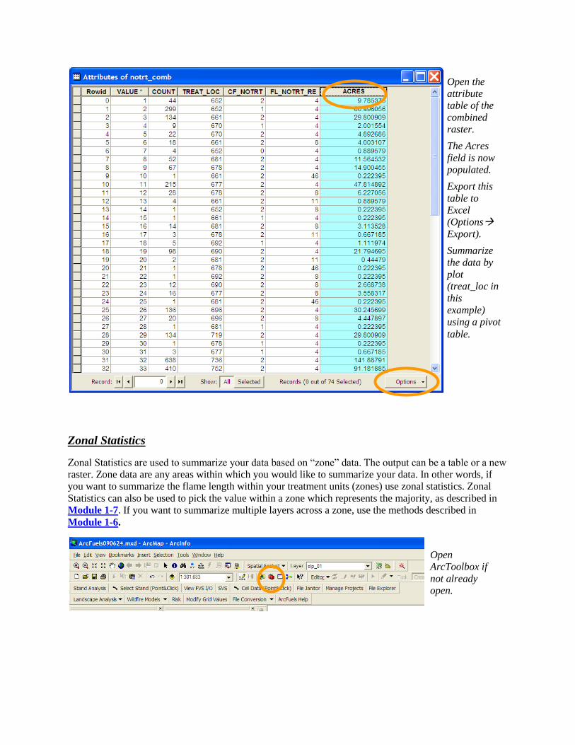
Zonal Statistics
Zonal Statistics are used to summarize your data based on “zone” data. The output can be a table or a new
raster. Zone data are any areas within which you would like to summarize your data. In other words, if
you want to summarize the flame length within your treatment units (zones) use zonal statistics. Zonal
Statistics can also be used to pick the value within a zone which represents the majority, as described in
Module 1-7. If you want to summarize multiple layers across a zone, use the methods described in
Module 1-6.
Open the
attribute
table of the
combined
raster.
The Acres
field is now
populated.
Export this
table to
Excel
(Options
Export).
Summarize
the data by
plot
(treat_loc in
this
example)
using a pivot
table.
Open
ArcToolbox if
not already
open.

Navigate to Spatial Analyst Tools Zonal.
Select “Zonal Statistics as Table”.

When the tool opens,
select the zone data
(i.e., treatment
units).
This can be a raster
or vector data layer.
The zone field is the
attribute within the
zone data layer you
would like to
summarize across
(i.e., treatment
units).
In the treat_loc file
value = treatment
units.
The Input Value
Raster is the raster
you would like to
summarize.
In this example, this
is pre-treatment,
unclassified flame
length.
Place a check mark
next to “Ignore
NoData”.
Navigate to a saving
location and name
the output table.
Click OK.

Select the Source tab to view your table in ArcMap.
Right-click on the zonal table and select, Open.
Alternatively, navigate to where you saved your table and open it
through Microsoft Excel. It will have a .dbf extension.

Examine the
table.
Value
represents
treatment unit.
In this
example, Unit
652 has a
minimum of 3,
maximum of 65
and average of
22 ft flame
lengths.
Navigate to Spatial Analyst Tools Zonal
Select “Zonal Statistics”.

When the tool opens, select
the zone data (i.e., treatment
units). This can be a raster or
vector data layer.
The zone field is the attribute
within the zone data layer
you would like to summarize
across (i.e., treatment units).
In the treat_loc file, value =
treatment units.
The Input value raster is the
raster you would like to
summarize.
In this example, haz_units =
hazard within treatment
units.
The Statistics type in this
example, “majority” creates
a new raster which identifies
each unit based on the
majority of hazard pixels.
Navigate to a saving location
and name the output table.
Click OK.
The resulting raster will look odd. As with any ArcMap raster
process, only the “VALUE” field is carried over.
In this example, the “Value” field is the haz_unit raster.
You will need to Join the resulting raster back to the original
hazard units raster to display the hazard classifications.
Continue to the next section for instructions related to this
process.

Post-Processing: Joining Attribute Tables of Raster Data
Often, the output from ArcMap raster processes
contains only a “Value” field.
This “Value” field is the link back to the
original data source and the associated
attribute table.
To re-attach the attribute table associated with
the output, it needs to be Joined back to the
original data source.
This example continues from the previous
section on Zonal Statistics.
Right-click on the raster which needs to be
Joined back to the original data source.
Select “Joins and Relates” and then “Join”.

From the drop down list, select “Join
attributes from a table”:
1. The field the Join will be based on is
the “Value” field,
2. The table to Join to this layer is
“haz_unit”, as this is where the
“Value” field originated from, and
3. Base the Join on the “Value”, as
this is the field which is common to
the output and the original data.
Keep only the matching records, since the
original data set contained more information
(rows of data) than the output.
Click OK.
Use the “Symbology” tab within the
Layer Properties to verify that the join
was successful.

Summarized data
Joined to original data
(left).
Original data (right).
To make the join permanent, right-click on the layer.
Select “Data” and then “Export Data”.

Exporting ArcGIS Data to Google Earth
If you want to share ArcGIS spatial data for public viewing in Google Earth there is an ArcToolbox tool
that will generate KML (keyhole markup language) files from ArcGIS layers. The files can then be
distributed or posted at a Google Earth site for viewing in Google Earth.
Open
ArcToolbox if
not already
open.
Verify the cell size.
Navigate to an output folder.
Rename the file (erase the
.img extension).
Select “Raster” from the
Format drop down list.
Click Save.

Navigate to Conversion Tools To KML
Layer To KML.
Select your layer to be converted
from the drop down list. Navigate to
an output location and name the file.
ArcMap creates a KMZ rather than a
KML, which is just a compressed
KML file. There is no need to
“decompress” it.
Choose a reasonably large layer
output scale. This determines the
scale at which you can see your file
in Google Earth
Click Ok.

In windows explorer, double-
click on your KMZ file. This
will automatically open
Google Earth.
These are the flow paths
from the demonstration data.
Alternatively, navigate to
your KMZ, by selecting File
Open.