architecture and implementation of database systems...
TRANSCRIPT

Architecture and Implementation
of Database Systems (Winter 2016/17)
Jens Teubner, DBIS Group
Winter 2016/17
© Jens Teubner · Architecture & Implementation of DBMS · Winter 2016/17 1

Part XII
Search
© Jens Teubner · Architecture & Implementation of DBMS · Winter 2016/17 534

Search
Ever-increasing amounts of data are available electronically.
These data have varying degrees of structure.
structured
information
un-structured
information
(R)DBMS unstructured text
XML
social graphs
text withmarkup
web pages
How can we efficiently store and access such un-structured data?
→ success of search engines ; “search”
© Jens Teubner · Architecture & Implementation of DBMS · Winter 2016/17 535

Boolean Queries
Let’s start with what we have. . .
E.g., four documents
Tropical fish in-
clude fish found
in tropical envi-
ronments around
the world, in-
cluding both
freshwater
and salt water
species.
doc1
Fishkeepers of-
ten use the term
tropical fish to
refer only those
requiring fresh
water, with salt-
water tropical
fish referred to
as marine fish.
doc2
Tropical fish are
popular aquar-
ium fish, due to
their often bright
coloration.
doc3
In freshwater
fish, this col-
oration typically
derives from iri-
descence, while
salt water fish
are generally pig-
mented.
doc4
Say we’re interested in “freshwater fish.”
→ Two search terms: “freshwater” and “fish”
© Jens Teubner · Architecture & Implementation of DBMS · Winter 2016/17 536
Boolean Queries
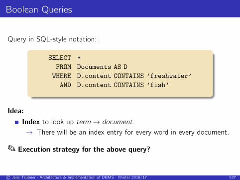
Query in SQL-style notation:
SELECT *
FROM Documents AS D
WHERE D.content CONTAINS ’freshwater’
AND D.content CONTAINS ’fish’
Idea:
Index to look up term → document.→ There will be an index entry for every word in every document.
� Execution strategy for the above query?
© Jens Teubner · Architecture & Implementation of DBMS · Winter 2016/17 537

Boolean Queries
Discussion:
Returns all documents that contain both search terms.
→ This may be more than we want.
Google: about 21 million pages with “freshwater” and “fish!”
Returns nothing else.
→ This may be less than we want.
doc2 and doc3 may be relevant for us, too.
Returns documents in no specific order.
→ But some documents might be more relevant than others.
→ ORDER BY won’t help!
Boolean Query: (exact match retrieval)
A predicate precisely tells whether a document belongs to the result.
Ranked Query:
Results are ranked according to their relevance (to the query).
© Jens Teubner · Architecture & Implementation of DBMS · Winter 2016/17 538

Ranking
Goal: Rank documents higher that are closer to the query’s intention.
→ Extract features from each document.
→ Use feature vector and query to compute a score.
Tropical fish include
fish found in tropical
environments around
the world, including
both freshwater and
salt water species.
document
9.7 fish
4.2 tropical
22.1 tropical fish
8.2 freshwater
2.3 species
topical features
14 incoming links
3 days since last upd.
quality features
“tropical fish”
query
ranking
function
303.01
document score
© Jens Teubner · Architecture & Implementation of DBMS · Winter 2016/17 539

Ranking
Idea:
Compute similarity between query and document.
Similarity:
Define a set of features to use for ranking.
→ each term in the collection is one feature
→ possible features: document size/age, page rank, etc.
For each document compute a feature vector di
→ e.g., yes/no features; term count; etc.
For the query compute a feature vector q.
Measure similarity of the two vectors.
© Jens Teubner · Architecture & Implementation of DBMS · Winter 2016/17 540

Vector Space Model
Two vectors are similar if the angle between them is small.
feature1
feature2
feature3
d1
d2
qCosine between di and q:
cos(di ,q) =
∑j dij · qj√∑
j d2ij ·∑
j q2j
(j iterates over all features/terms;
i is the document in question)
→ “vector space model”
© Jens Teubner · Architecture & Implementation of DBMS · Winter 2016/17 541

Ranking Model
Ignoring the normalization term: sim(di ,q) =∑
j dijqj .
→ Multiply corresponding feature values, then sum up.
Tropical fish in-
clude fish found
in tropical envi-
ronments around
the world, includ-
ing both freshwa-
ter and salt water
species.
document
9.7 fish
4.2 tropical
22.1 tropical fish
8.2 freshwater
2.3 species
topical features
14 incoming links
3 days last upd.
quality features
“tropical fish”
query
fish 5.2
tropical 3.4
tropical fish 9.9
chichlids 1.2
barbs 0.7
topical features
incoming links 1.2
days last upd. 0.9
quality features
303.01document score
� What does this mean for an implementation?
© Jens Teubner · Architecture & Implementation of DBMS · Winter 2016/17 542

tf /idf Ranking
What are good features (and their values)?
Topical Features:
Each term in the collection (; vocabulary) is one feature.
Feature Value:
A document with multiple occurrences of ‘foo’ is likely more
relevant to queries that contain ‘foo’.
→ term frequency tf as a feature value.
tf doc,foo =number of occurrences of ‘foo’ in doc
number of words in doc
→ Normalize to account for different document sizes.
© Jens Teubner · Architecture & Implementation of DBMS · Winter 2016/17 543

tf /idf Ranking
Terms that occur in many documents are less discriminating.
→ inverse document frequency idf :
idf foo = lognumber of documents in the collection
number of documents that contain ‘foo’
→ idf is a property of the term, not the document!
Combine to obtain feature value dij (document i , term j):
dij = tf ij · idf j .
Do the same thing for query features qj .
© Jens Teubner · Architecture & Implementation of DBMS · Winter 2016/17 544
tf /idf Ranking
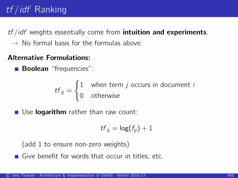
tf /idf weights essentially come from intuition and experiments.
→ No formal basis for the formulas above.
Alternative Formulations:
Boolean “frequencies”:
tf ij =
{1 when term j occurs in document i
0 otherwise
Use logarithm rather than raw count:
tf ij = log(fij) + 1
(add 1 to ensure non-zero weights)
Give benefit for words that occur in titles, etc.
© Jens Teubner · Architecture & Implementation of DBMS · Winter 2016/17 545

Quality Features
Some document characteristics do not tell whether the document
matches the subject of a query.
→ Yet they may be relevant to the ranking/quality of the document.
Examples:
Web pages with higher incoming link count may more trustworthy.
Documents that weren’t modified for a long time may contain
outdated information.
Quality features for the query may help to express the user’s intention:
Is (s)he only interested in the most recent news?
→ Give higher weight to features like ‘days last updated’.
© Jens Teubner · Architecture & Implementation of DBMS · Winter 2016/17 546

PageRank
PageRank28 is a quality feature that became popular with the rise of
Google.
Motivation: Use link analysis to rate the popularity of a web site.
→ Incoming links indicate quality, but are easy to manipulate.
→ Try to weigh each incoming link by the popularity of the originating
site.
Idea:
Assume a random Internet surfer Alice.
→ On every page, randomly click some of its outgoing links.
→ Every now and then (with probability λ) jump to a random
page instead.
PageRank of a page p: What is the probabilty that Alice looks at p
when we randomly interrupt her browsing?
28Named after Google founder Larry Page.© Jens Teubner · Architecture & Implementation of DBMS · Winter 2016/17 547

Computing PageRank
Example:
A B
C
Probability that Alice ends up on C :
PR(C ) =λ
3︸︷︷︸random jump
+ (1− λ) ·(PR(A)
2+PR(B)
1
)︸ ︷︷ ︸
chance of coming from A or B
.
Generally:
PR(u) =λ
N+ (1− λ) ·
∑v∈Bu
PR(v)
outgoingv.
© Jens Teubner · Architecture & Implementation of DBMS · Winter 2016/17 548

Computing PageRank
But we don’t know PR(A) and PR(B), yet!
→ Iterate the above formula and PageRanks will converge.
→ E.g., initialize with equal PageRanks 1/N.
A typical value for λ is 0.15.
Today, PageRank is just one out of many features used in ranking.
→ Tends to have most impact on popular queries.
© Jens Teubner · Architecture & Implementation of DBMS · Winter 2016/17 549

Prepare for Queries
Before querying, documents must be analyzed:
1 Parse and tokenize document.
→ Strip markup (if applicable), identify text to index.
→ Break text into tokens (words).
→ Normalize capitalization.
2 Remove stop words.
→ ‘the,’ ‘a,’ ‘this,’ ‘that,’ etc. generally not useful for search.
3 Normalize words to terms (“stemming”).
→ E.g., ‘fishing,’ ‘fished,’ ‘fisher’ → ‘fish’
→ Stems need not themselves be words (e.g., ‘describe,’
‘describing,’ ‘description’ → ‘describ’)
4 Some systems also extract phrases.
→ E.g., ‘european union,’ ‘database conference’
Terms are then used to populate an index.
© Jens Teubner · Architecture & Implementation of DBMS · Winter 2016/17 550

Inverted Files
A search engine’s document collection is essentially a mapping
document → list of term .
To search the collection, it is much more useful to construct the mapping
term → list of document .
E.g.,
term docs
and (doc1)
aquarium (doc3)
are (doc3, doc4)
around (doc1)
as (doc2)
term docs
both (doc1)
bright (doc3)
coloration (doc3, doc4)
derives (doc4)
due (doc3)
© Jens Teubner · Architecture & Implementation of DBMS · Winter 2016/17 551

Inverted Files
A representation of this type is thus also called inverted file29.
Conceptually, an inverted file is the same as a database index.
However, in a search engine, the inverted file forms the heart of the
whole system.
→ It makes sense to specialize and fine-tune its implementation.
→ Terminology: For each index term there’s one inverted list.
The inverted list is a list of postings.
Characteristics:
The set of index terms is pretty much fixed (e.g., given by the
English dictionary).
Sizes of inverted lists, by contrast, grow with the number of
documents indexed.
→ Their sizes typically follow a Zipfian distribution.
29sometimes also “inverted index”© Jens Teubner · Architecture & Implementation of DBMS · Winter 2016/17 552

Size of Inverted Files
Inverted files can grow large.
→ One posting for every term in every document.
→ Index about as large as entire document collection.
It thus makes sense to compress inverted lists.
� How well will lists of document ids compress?
→ Inverted list a “random” subset of all document ids, with uniform
probability.
→ Little entropy to use for compression.
© Jens Teubner · Architecture & Implementation of DBMS · Winter 2016/17 553

Inverted Files—Compression
This changes if we sort, then delta-encode inverted lists:
1, 5, 9, 18, 23, 24, 30, 44, 45, 48
;
1, 4, 4, 9, 5, 1, 6, 14, 1, 3
Can now use compression schemes that favor small values.
→ E.g., null suppression
Suppress leading null bytes.
Encode number of suppressed nulls with fixed-length prefix.
E.g., 18 → 00 00010010; 427 → 01 00000001 10101011.
→ E.g., unary codes
Encode n with sequence of n 1s, followed by a 0.
E.g., 0 → 0; 1 → 10; 2 → 110; 12 → 1111111111110.
© Jens Teubner · Architecture & Implementation of DBMS · Winter 2016/17 554

Inverted Files—Elias-γ Compression
Elias-γ Codes:
To encode n, compute
nd = blog2 nc “position of leading bit”
nr = n − 2blog2 nc “value encoded by remaining bits”
Then, represent n using
nd , unary-encoded; followed by
nr , binary-encoded.
n nd nr code
1 0 0 0
2 1 0 10 0
3 1 1 10 1
15 3 7 1110 111
255 7 127 11111110 1111111
© Jens Teubner · Architecture & Implementation of DBMS · Winter 2016/17 555

Inverted Files—PFOR Compression
PFOR Compression:
Illustrated here using compressed representation of the digits of π.30
header 3 1
4 1 5 2 6 5 3 5
3 2
⊥ ⊥⊥ ⊥ ⊥
9 7 9 8 9
compressed data
exceptions
Decompressed numbers: 31415926535897932
30PFOR was developed in the context of the MonetDB/X100 main-memory
database project, now commercialized by Actian.© Jens Teubner · Architecture & Implementation of DBMS · Winter 2016/17 556

PFOR Decompression
During decompression, we have to consider all the exceptions:
for (i = j = 0; i < n; i++)
if (code[i] != ⊥)output[i] = DECODE (code[i]);
else
output[i] = exception[--j];
For PFOR, DECODE is a simple addition:
#define DECODE(a) ((a) + base value)
Problem on modern hardware: High branch misprediction cost.
© Jens Teubner · Architecture & Implementation of DBMS · Winter 2016/17 557

PFOR: Avoiding the Misprediction Cost
Invest some unnecessary work to avoid high misprediction penalty.
Run decompression in two phases:
1 Decompress all regular fields, but don’t care about exceptions.
2 Work in all the exceptions and patch the result.
/* ignore exceptions during decompression */
for (i = 0; i < n; i++)
output[i] = DECODE (code[i]);
/* patch the result */
foreach exception
patch corresponding output item ;
© Jens Teubner · Architecture & Implementation of DBMS · Winter 2016/17 558

PFOR: Patching the Output
�We don’t want to use a branch to find all exception targets!
Thus: interpret values in “exception holes” as linked list:
header 3 1
4 1 5 2 6 5 3 5
7 3 2
5 0
1 3
9 9 8 9
compressed data
exceptions
→ Can now traverse exception holes and patch in exception values.
© Jens Teubner · Architecture & Implementation of DBMS · Winter 2016/17 559

PFOR: Patching the Output
The resulting decompression routine is branch-free:
/* ignore exceptions during decompression */
for (i = 0; i < n; i++)
output[i] = DECODE (code[i]);
/* patch the result (traverse linked list) */
j = 0;
for (cur = first exception; cur < n; cur = next) {next = cur + code[cur] + 1;
output[cur] = exception[--j];
}
© Jens Teubner · Architecture & Implementation of DBMS · Winter 2016/17 560

Query Execution—Boolean Queries
With inverted lists available, the evaluation of
term1 and term2
amounts to computing the intersection of the two inverted lists.
Strategy: (assuming inverted lists are sorted by document id)
→ “Merge” lists lterm1 and lterm2 (↗ merge join (), slide 186).
→ Cost: linear scan of lterm1 plus linear scan of lterm2 .
Problem: Long, inefficient scans
E.g.,
|lfish| = 300 M; |lfreshwater | = 1 M.
At least 299 M lfish entries scanned unnecessarily.
→ Skip over those entries?
© Jens Teubner · Architecture & Implementation of DBMS · Winter 2016/17 561

Skip Pointers
Idea:skip pointers postings
Skip pointers point to every kth posting.
skip pointer: 〈byte pos, doc id〉.
Skip forward to document d :
1 Read skip pointer list as long as doc id ≤ d .
2 Follow the pointer and scan posting list from there to find d .
© Jens Teubner · Architecture & Implementation of DBMS · Winter 2016/17 562

Skip Pointers
Example: |lfish| = 300 M; |lfreshwater | = 1 M; skip distance k .
For complete merge: (cost to read lfish)
Read all 300 M/k skip pointers.
Perform 1 M posting list scans; average length: 12k .
Total cost to read lfish: 300,000,000/k + 500,000k :
0 M
20 M
40 M
60 M
0 20 40 60 80 100
cost
k
© Jens Teubner · Architecture & Implementation of DBMS · Winter 2016/17 563

Skip Pointers
Improvements:
Rather than reading skip pointer list sequentially, use
→ binary search,
→ exponential search (also: “galloping search”), or
→ interpolation search.
� Why not use these search methods directly on the inverted list?
Compression makes skipping really difficult.
For delta-encoded data, need to know previous value to decode.
© Jens Teubner · Architecture & Implementation of DBMS · Winter 2016/17 564

Query Execution (with Ranking)
Idea:
1 Compute score for each document.
2 Sort by score.
3 Return top n result documents.
Only features j where qj 6= 0 will contribute to∑
j dijqj .
→ Score only documents that appear in at least one inverted list for
the index terms in q.
© Jens Teubner · Architecture & Implementation of DBMS · Winter 2016/17 565

Term-at-a-Time Retrieval
Process inverted lists one after another:
1 R ← PriorityQueue (n) ;
2 A← HashTable () ;
3 foreach term j in q do
4 foreach document i in inverted list for j do
5 score ← A.get (i) ;
6 if not found then
7 A.put (i , dijqj ) ;
8 else
9 A.put (i , score + dijqj ) ;
10 foreach 〈i , score〉 in A do
11 R.add (i , score) ;
12 return R ;
© Jens Teubner · Architecture & Implementation of DBMS · Winter 2016/17 566

Document-at-a-Time Retrieval
1 R ← PriorityQueue (n) ;
2 foreach term j in q do
3 L.add (inverted list for j) ;
4 while L is not empty do
/* Find next document i in any inverted list */
5 i ← smallest lj .docID in L ;
/* Score document i */
6 score ← 0 ;
7 foreach lj ∈ L do
8 if lj .docID = i then
9 score ← score + dijqj ;
10 lj .advance () ;
11 if eof (lj ) then
12 L.remove (lj ) ;
13 R.add (i , score) ;
14 return R ;
© Jens Teubner · Architecture & Implementation of DBMS · Winter 2016/17 567

Optimizations: Conjunctive Processing
Restriction:
Return only documents that contain all of the query terms.
Then:
Document-at-a-time ; intersection/merging.
→ Use skip lists to navigate through inverted lists quickly.
In k-way merges, it may help to always consult shortest inverted
list first.
�This is a heuristic and might miss some top-n results!
© Jens Teubner · Architecture & Implementation of DBMS · Winter 2016/17 568

Threshold Methods: MaxScore
Top-n formulation returns only documents with score ≥ τ .
→ But we know τ only after we evaluated the query!
However:
Once we added n elements to the priority queue R, we can conclude
that
τ ≥ τ ′def= minimum score in R .
i.e., τ ′ is a conservative estimate for τ .
For each inverted list lj , maintain maximum score µj .
→ Once τ ′ > µj , documents that occur only in lj can be skipped.
MaxScore achieves similar effect as conjunctive processing, but
guarantees a correct result.
© Jens Teubner · Architecture & Implementation of DBMS · Winter 2016/17 569
List Ordering
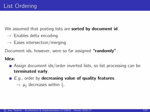
We assumed that posting lists are sorted by document id.
→ Enables delta encoding.
→ Eases intersection/merging.
Document ids, however, were so far assigned “randomly”.
Idea:
Assign document ids/order inverted lists, so list processing can be
terminated early.
E.g., order by decreasing value of quality features.
→ µj decreases within lj .
© Jens Teubner · Architecture & Implementation of DBMS · Winter 2016/17 570

Inverted Lists with More Details
So far:
Inverted lists contain document ids (pointers to documents).
Must read (maybe even parse, tokenize, stem) documents to get qij .
Instead:
Add information to inverted lists to avoid document access.
Example: Add
number of documents that contain the term (; idf j )
number of occurrences of the term in the document (; tf ij )
term # docs
and 1 (〈doc1:1〉)aquarium 1 (〈doc3:1〉)are 2 (〈doc3:1〉, 〈doc4:1〉)around 1 (〈doc1:1〉)as 1 (〈doc2:1〉)
term # docs
both 1 (〈doc1:1〉)bright 1 (〈doc3:1〉)coloration 2 (〈doc3:1〉, 〈doc4:1〉)derives 1 (〈doc4:1〉)due 1 (〈doc3:1〉)
© Jens Teubner · Architecture & Implementation of DBMS · Winter 2016/17 571
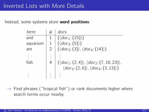
Inverted Lists with More Details
Instead, some systems store word positions:
term # docs
and 1 (〈doc1: (15)〉)aquarium 1 (〈doc3: (5)〉)are 2 (〈doc3: (3)〉, 〈doc4: (14)〉)...
......
fish 4 (〈doc1: (2, 4)〉, 〈doc2: (7, 18, 23)〉,〈doc3: (2, 6)〉, 〈doc4: (3, 13)〉)
......
...
→ Find phrases (“tropical fish”) or rank documents higher where
search terms occur nearby.
© Jens Teubner · Architecture & Implementation of DBMS · Winter 2016/17 572

Inverted Lists with More Details
Store tf ij idf i directly in inverted list?
" Speeds up computation of document scores.
→ Could incorporate even more expensive offline computations.
% Very inflexible.
→ What if ranking function changes? Need to re-compute index!
% Scoring values might compress poorly.
More Tricks:
Store extent lists as inverted lists:
→ E.g., inverted list for ‘title’, storing document regions that
correspond to the document’s title.
→ Fits well with start/end tags in markup languages.
© Jens Teubner · Architecture & Implementation of DBMS · Winter 2016/17 573

Evaluating a Search Engine
A good search engines returns
many relevant documents, but
few non-relevant documents.
“Relevant”?
What matters is relevance to the user.
To evaluate a search engine
→ Take a test collection of documents and queries.
→ Obtain relevance judgements from experts (users).
→ Compare search engine output to expert judgements.
© Jens Teubner · Architecture & Implementation of DBMS · Winter 2016/17 574

Recall and Precision
Recall:
How many of the relevant documents were retrieved?
Recall =|retrieved documents that are relevant|
|all relevant documents|
Precision:
How many of the retrieved documents are relevant?
Precision =|retrieved documents that are relevant|
|retrieved documents|Since we return top-n documents according to rank, both values will vary
with n.
© Jens Teubner · Architecture & Implementation of DBMS · Winter 2016/17 575

Recall and Precision
Precision and recall for an example document/query:
relevant documents
0 %
25 %
50 %
75 %
100 %
0 5 10 15 20 resultdocument
© Jens Teubner · Architecture & Implementation of DBMS · Winter 2016/17 576

Recall and Precision
Recall is monotonically
increasing.
Precision tends to
decrease with n.
→ Draw “recall-precision
graph”
0 %0 %
25 %
25 %
50 %
50 %
75 %
75 %
100 %
100 %
Recall
Pre
cisi
on
© Jens Teubner · Architecture & Implementation of DBMS · Winter 2016/17 577