1

Armington Meets Melitz: Introducing Firm Heterogeneity in Global

CGE Model of Trade

Fan Zhai+

December 23, 2006

Abstract

Traditional CGE models with Armington assumption fail to capture the extensive margin of trade, thereby underestimate the trade and welfare effects of trade opening. To address this problem, this paper introduces the Melitz (2003) theoretical framework with firm heterogeneity and fixed exporting costs into a global CGE model. Some illustrative simulations show that the introduction of firm heterogeneity improves the ability of CGE model to capture the trade expansion and welfare effects of trade liberalization. Under the case of global manufacturing tariff cut, the estimated gains in welfare and exports are more than double of that obtained from standard Armington CGE model. Sensitivity analysis also indicates that model results are sensitive to the shape parameters of firm productivity distribution, suggesting the need of further empirical work to estimate the degree of firm heterogeneity.

+ Economist, Asian Development Bank, Tel: +632-632-5956, Email: fzhai@adb.org

2

1. Introduction

Computable General Equilibrium (CGE) models have been used extensively in trade policy analysis.

Despite shedding considerable light on static welfare effects and structural adjustment of trade reform

around the world, however, CGE models fail to capture some important features in modern international

trade1. The most striking one is the extensive margin, i.e. the number of exporting firms and traded

goods. In the standard CGE model with Armington’s (1969) national product differentiation, trade is

expanded purely at the intensive margin: each exporter increases the size of its exports, but there is no

change in the set of exporters. However, recent research has revealed the significant importance of the

extensive margin for international trade. Empirical studies show that larger countries trade not only

bigger size, but also wider variety of goods. Using data on shipment by 126 exporting countries to 59

importing countries in 5,000 product categories, Hummels and Klenow (2005) find that the extensive

margin account for 60% of the greater of exports of larger economies, and about one third of the greater

imports of the same countries. Eaton, Kortum and Kramarz (2004) examine the firm-level export data of

French firms and conclude that the number of exporting firms, rather than the amount exported by each

firm, determines the variation in French exports across destinations. Extensive margin is also a crucial

force to drive the trade expansion following trade liberalizations. In a study of six different trade

liberalizations, Kehoe and Ruhl (2003) find that trade in goods that were not before traded shows

substantial growth following a decrease in trade barriers. The set of goods that accounted for only 10%

percent of trade before the liberalization may account for 40% of trade following the liberalization.

The absence of extensive margin makes the trade CGE models incapable to explain the fast world

trade growth since 1960s, leading to the quantitative puzzle of why modest decreases in tariffs generate

strong expansion in trade (Bergoeing and Kehoe, 2001; Yi, 2003). For example, Kehoe (2005) uses data

on actual changes in trade flows among Canada, the US and Mexico between 1988 and 1999 to evaluate

1 See Devarajan and Robinson (2005) on the influence of CGE models on trade policy and Kehoe (2005) for a critical review of

3

the performance of three CGE models that were used in the early 1990s to estimate the impacts of

NAFTA. He finds that these models dramatically underestimated the impact of NAFTA on the volume of

regional trade, especially for Mexico. Mexico’s regional trade relative to GDP increased by over 1,000%

in many sectors between 1988 and 1999, while the CGE models predicted changes in trade relative to

GDP of less than 50% in most sectors.

The absence of extensive margin in Armington-type CGE models also results in the well-known

“stuck on zero trade” problem (Abler, 2006; Kuiper and van Tongeren, 2006). As Kehoe (2005) argued,

the Armington specification has the effect of locking in pre-existing trade patterns and prevented the

models from generating large changes in trade in sectors where little or no trade. Under this specification,

a country’s imports of a product from another country are zero initially they will always be zero, even

after significant reductions of trade barriers. If imports are nonzero but small they will remain small even

if there are large changes in prices. This “stuck on zero trade” problem makes CGE models especially

inappropriate for the least developed countries which usually have limited trade with the rest of the

world.

Extensive trade margin has important implication for evaluating the welfare effects of trade

liberalization. In CGE models with national products differentiation, the simulated welfare changes of

trade liberalization are dominated by the terms-of-trade effects associated with the intensive export

growth, i.e. expanding export quantity but lower export price of each variety (Brown, 1987). However,

as mentioned by Hummels and Klenow (2005), if export expansion is based more on extensive margin or

high quality, such adverse terms-of-trade effects are no longer a necessary consequence.

Recently, a number of new heterogeneous-firm models of international trade by Bernard, Eaton,

Jensen and Kortum (2003), Melitz (2003), and Yeaple (2005) have introduced the extensive margin as a

result of the firms’ self-selection to export markets. They emphasis the interaction of trade costs and

CGE analysis of NAFTA.

4

productivity differences across firms operating in imperfectly competitive industries. The existence of

trade costs induce only most productive firms to self-select into export markets. When trade costs

decrease, new firms with lower productivity enter the export markets in response to the potential higher

profits. On the other hand, the least productivity non-exporting firms are forced to exit because of the

increased import competition in domestic markets. Empirical evidences have largely supported the

predictions by the new firm-heterogeneity trade models2.

An attractive feature of the new firm-heterogeneity trade models is that they provide an explicit

microeconomic channel through which trade liberalization boosts aggregate productivity. Under these

models, productivity gains via the reallocation of economic activity across firms within industry, as low

productivity firms would exit and high productivity exporting firms would expand their market shares

following the trade liberalization. The productivity effects of trade liberalization are key factors to

understand the impact of trade liberalization, but, are often missed in most CGE models3.

In order to improve the ability of applied trade models to describe the trade facts, this paper attempts

to incorporate the recent development in heterogeneous-firm trade models into a global CGE model.

Specially, I implement a firm heterogeneity global CGE model based on Melitz (2003), and carry out

experimental simulations to illustrate its features. The reminder of the paper is organized as follows: the

next section presents the Melitz(2003) model. Section 3 discusses the specification of the heterogeneous

firm CGE model and its calibration. Section 4 presents the simulation results of trade liberalization using

the new CGE model, and compares them to those obtained from standard Armington-type CGE model.

Section 5 conducts sensitivity analysis. The final section offers conclusions.

2 Chaney (2006) estimates the distorted gravity equations based on a simplified version of Melitz (2003) model, and found strong

support for it in both sectoral trade data and the stylized facts on firm-level trade. Bernard, Jensen and Schott (2006) use the firm level US manufacturing data to examine the effects of changing trade costs on firms’ entry and exit behavior and changes in average productivity. They find that lowering trade costs in a sector increases the probability of firm death or entering export markets in that sector. The existing exports would expand as trade costs decline. Moreover, industry aggregate productivity and within-plant productivity rise as trade costs fall.

3 Some CGE models incorporate ad hoc assumptions about trade-productivity externalities, such as linking productivity to export

performance or imported intermediate and capital goods. See, for example, de Melo and Robinson (1992), Lewis, Robinson and Wang (1995) and World Bank (2001).

5

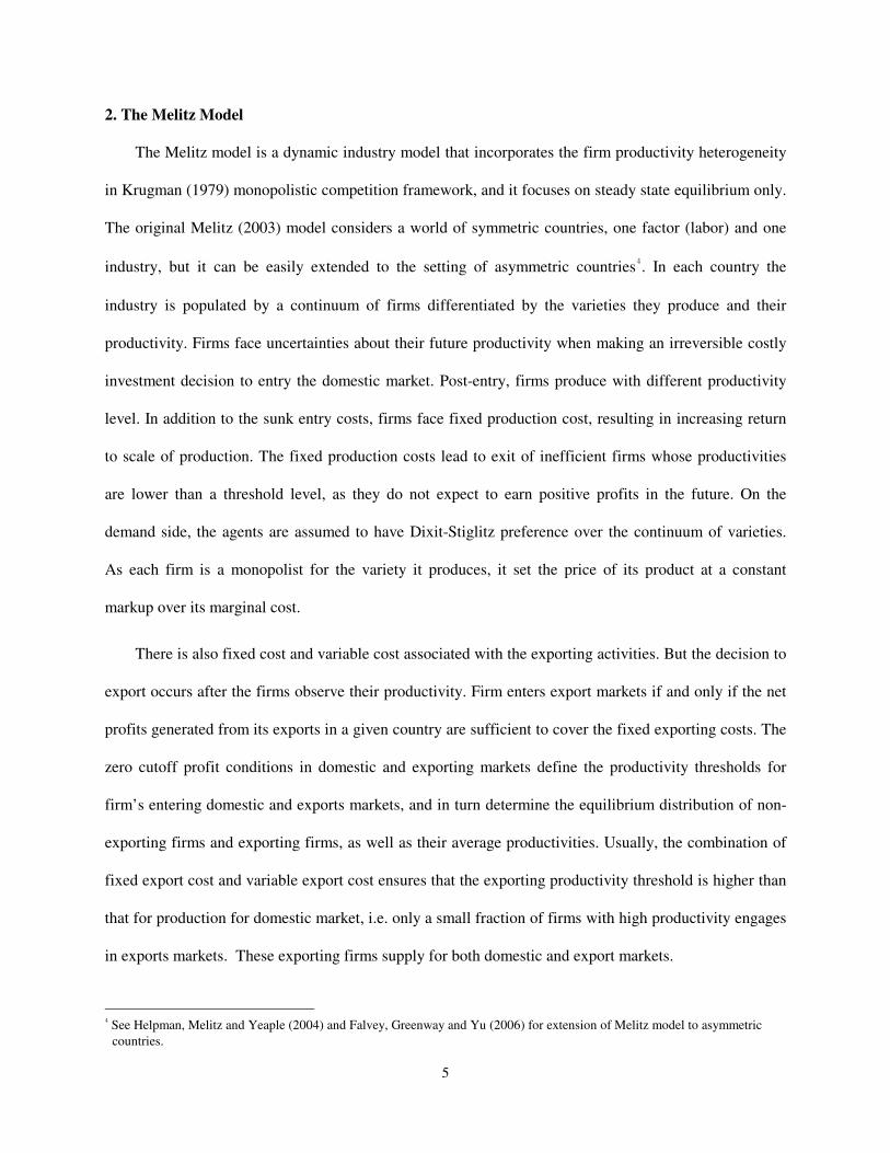
2. The Melitz Model

The Melitz model is a dynamic industry model that incorporates the firm productivity heterogeneity

in Krugman (1979) monopolistic competition framework, and it focuses on steady state equilibrium only.

The original Melitz (2003) model considers a world of symmetric countries, one factor (labor) and one

industry, but it can be easily extended to the setting of asymmetric countries4. In each country the

industry is populated by a continuum of firms differentiated by the varieties they produce and their

productivity. Firms face uncertainties about their future productivity when making an irreversible costly

investment decision to entry the domestic market. Post-entry, firms produce with different productivity

level. In addition to the sunk entry costs, firms face fixed production cost, resulting in increasing return

to scale of production. The fixed production costs lead to exit of inefficient firms whose productivities

are lower than a threshold level, as they do not expect to earn positive profits in the future. On the

demand side, the agents are assumed to have Dixit-Stiglitz preference over the continuum of varieties.

As each firm is a monopolist for the variety it produces, it set the price of its product at a constant

markup over its marginal cost.

There is also fixed cost and variable cost associated with the exporting activities. But the decision to

export occurs after the firms observe their productivity. Firm enters export markets if and only if the net

profits generated from its exports in a given country are sufficient to cover the fixed exporting costs. The

zero cutoff profit conditions in domestic and exporting markets define the productivity thresholds for

firm’s entering domestic and exports markets, and in turn determine the equilibrium distribution of non-

exporting firms and exporting firms, as well as their average productivities. Usually, the combination of

fixed export cost and variable export cost ensures that the exporting productivity threshold is higher than

that for production for domestic market, i.e. only a small fraction of firms with high productivity engages

in exports markets. These exporting firms supply for both domestic and export markets.

4 See Helpman, Melitz and Yeaple (2004) and Falvey, Greenway and Yu (2006) for extension of Melitz model to asymmetric

countries.

6

The remaining of this section describes detailed specification of the model. For notational

simplicity, the region subscript i is omitted in what follows if this does not lead to confusion.

(1) Demand

There are R countries in the world. In each country, the representative consumer maximizes utility

from consumption over a continuum of goods Ω. The utility U, or the aggregate good Q, is described by

CES function,

( )11 −

Ω∈

−

== ∫

σ

σ

ωσ

σ

ωqQU (1)

where ωq is the quantity of consumption of good ω, σ is the substitution elasticity across goods. The

dual price index of utility P is defined over the prices of each good, ωp ,

( )( ) σ

ω

σω −

Ω∈

−

∫= 1

11

pP (2)

And the demand for each good is

( )( )

σ

ωω

=

p

PQq (3)

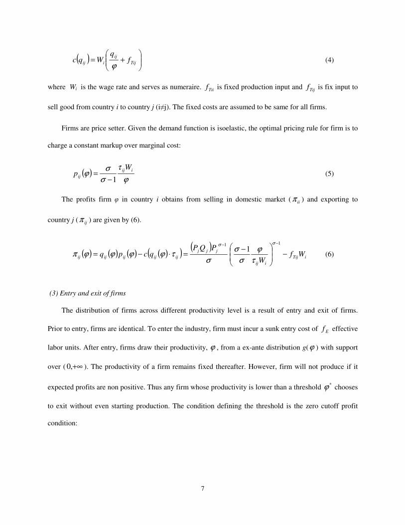
(2) Production and trade

There is a continuum of firms in each country, each with different productivity φ and producing a

different variety ω. Production involves a fixed and variable cost, and requires only factor, labor. Trade

is assumed costly. A firm must pay a fixed cost to export. In addition, there are variable trade costs,

which take the form of iceberg transportation cost whereby only a fraction 1/ ijτ arrives for shipping one

unit of good from country i to j ( ijτ =1 for i=j). Thus, for a firm with productivity φ, the cost of

producing q units of good ω and selling them to country j is:

7

( )

+= Tij

ij

iij fq

Wqcϕ

(4)

where Wi is the wage rate and serves as numeraire. Tiif is fixed production input and Tijf is fix input to

sell good from country i to country j (i≠j). The fixed costs are assumed to be same for all firms.

Firms are price setter. Given the demand function is isoelastic, the optimal pricing rule for firm is to

charge a constant markup over marginal cost:

( )ϕ

τ

σ

σϕ

iij

ij

Wp

1−= (5)

The profits firm φ in country i obtains from selling in domestic market ( iiπ ) and exporting to

country j ( ijπ ) are given by (6).

( ) ( ) ( ) ( )( )( )

iTij

iij

jjj

ijijijijij WfW

PQPqcpq −

−=⋅−=

−− 111

σσ

τ

ϕ

σ

σ

στϕϕϕϕπ (6)

(3) Entry and exit of firms

The distribution of firms across different productivity level is a result of entry and exit of firms.

Prior to entry, firms are identical. To enter the industry, firm must incur a sunk entry cost of Ef effective

labor units. After entry, firms draw their productivity, ϕ , from a ex-ante distribution g(ϕ ) with support

over ( +∞,0 ). The productivity of a firm remains fixed thereafter. However, firm will not produce if it

expected profits are non positive. Thus any firm whose productivity is lower than a threshold *ϕ chooses

to exit without even starting production. The condition defining the threshold is the zero cutoff profit

condition:

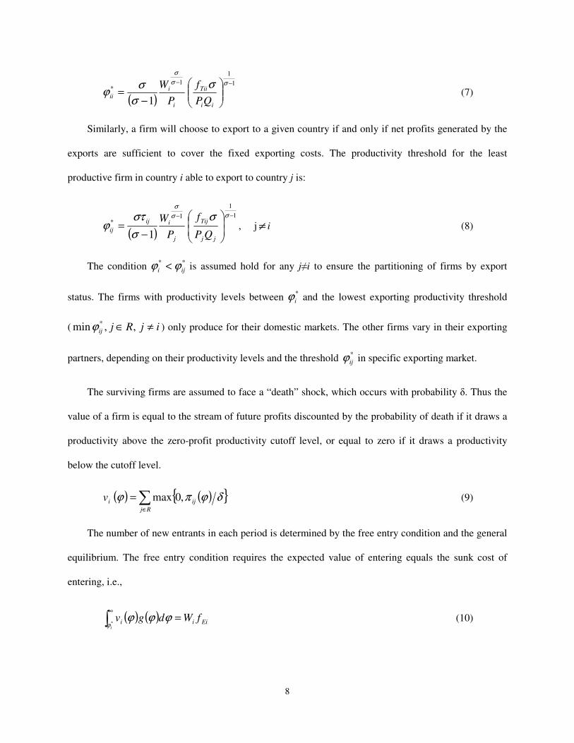
8

( )

1

1

1*

1

−−

−=

σσ

σ

σ

σ

σϕ

ii

Tii

i

i

iiQP

f

P

W (7)

Similarly, a firm will choose to export to a given country if and only if net profits generated by the

exports are sufficient to cover the fixed exporting costs. The productivity threshold for the least

productive firm in country i able to export to country j is:

( )

1

1

1*

1

−−

−=

σσ

σ

σ

σ

στϕ

jj

Tij

j

iij

ijQP

f

P

W, j≠i (8)

The condition **

iji ϕϕ < is assumed hold for any j≠i to ensure the partitioning of firms by export

status. The firms with productivity levels between *

iϕ and the lowest exporting productivity threshold

( ijRjij ≠∈ ,,min *ϕ ) only produce for their domestic markets. The other firms vary in their exporting

partners, depending on their productivity levels and the threshold *

ijϕ in specific exporting market.

The surviving firms are assumed to face a “death” shock, which occurs with probability δ. Thus the

value of a firm is equal to the stream of future profits discounted by the probability of death if it draws a

productivity above the zero-profit productivity cutoff level, or equal to zero if it draws a productivity

below the cutoff level.

( ) ( ) ∑∈

=Rj

ijiv δϕπϕ ,0max (9)

The number of new entrants in each period is determined by the free entry condition and the general

equilibrium. The free entry condition requires the expected value of entering equals the sunk cost of

entering, i.e.,

( ) ( ) Eiii fWdgvi

=∫∞

*ϕϕϕϕ (10)

9

And in steady state equilibrium, the mass of firms entering and producing must equal the mass of firms

that die. Using Me to denote the mass of new entrants and M to denote the mass of incumbents, the

equilibrium condition is

( ) MMG e δϕ =− )(1 * (11)

where )(ϕG is the cumulative distribution function of )(ϕg , and in 1- )( *ϕG is the ex ante probability

of successful entry in the industry.

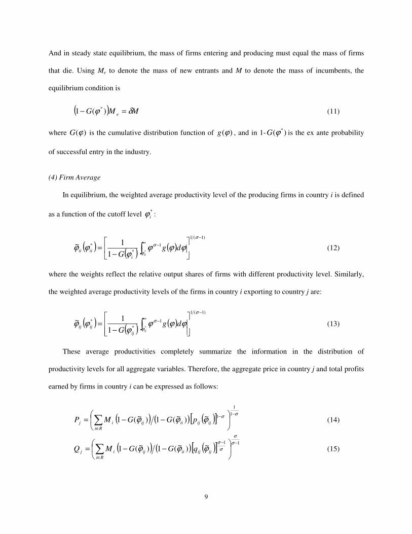
(4) Firm Average

In equilibrium, the weighted average productivity level of the producing firms in country i is defined

as a function of the cutoff level *

iϕ :

( )( )

( ))1(1

1

*

*

*

1

1~−

∞−

−= ∫

σ

ϕ

σ ϕϕϕϕ

ϕϕii

dgG i

iiii (12)

where the weights reflect the relative output shares of firms with different productivity level. Similarly,

the weighted average productivity levels of the firms in country i exporting to country j are:

( )( )

( ))1(1

1

*

*

*

1

1~−

∞−

−= ∫

σ

ϕ

σ ϕϕϕϕ

ϕϕij

dgG ij

ijij (13)

These average productivities completely summarize the information in the distribution of

productivity levels for all aggregate variables. Therefore, the aggregate price in country j and total profits

earned by firms in country i can be expressed as follows:

( ) ( ) ( )[ ]σ

σϕϕϕ

−

∈

−

−−= ∑

1

1

1~)~(1)~(1Ri

ijijiiijij pGGMP (14)

( ) ( ) ( )[ ]11

~)~(1)~(1−

∈

−

−−= ∑

σ

σ

σ

σ

ϕϕϕRi

ijijiiijij qGGMQ (15)

10

( ) ( ) ( )∑∈

−−=ΠRj

ijijiiijii GGM ϕπϕϕ ~)~(1)~(1 (16)

5) Equilibrium

In each country, the representative consumer supplies L units of labor. The equilibrium in labor

market requires that:

( ) ( ) ( ) Eie

Rj

Tijiiiji

j

ijijijEiPii fMfGGMqLLL +−−+=+= ∑∑∈

)~(1)~(1~~ ϕϕϕϕ (17)

where Lp is the labor input for production and Le is that used in investment by new entrants.

The representative consumer receives labor income and profits, and spends on consumption Q and

irreversible investment Ef . As the free entry ensures that total profits are exhausted by the aggregate

investment sunk costs of new entrants, i.e., ( )

Π=−

== Ei

ii

EieEi fG

MfML

)(1 *ϕ

δ, the budget constraint

of consumer is QPLW ⋅=⋅ . This budget constraint also determines the equilibrium in goods market in

each country.

6) Properties of the equilibrium

Some properties of the equilibrium of the model are worthy mentioning. First, trade opening leads to

reallocation of market shares and profits among firms. Falling trade costs increases the profits of

exporting firms and lowers the exporting productivity threshold. As a result, new and less productive

firms enter the export markets. Moreover, reduction of trade costs enables existing exporting firms to

increase their sales to foreign markets. In domestic market, more competition from increased imports

results in domestic firms losing a portion of their domestic markets. One the other hand, the expansion of

existing high productivity firms for exports and the entry of new firms increase labor demand, driving up

real wage. Reduced profits and rising costs make the less productive firms unable to survive, forcing

11

them to exit. As a result, the most productive firms increase their market shares and profits, while the

least productivity firms shrink or exit. Thus, trade opening leads to larger inequalities between firms.

Second, because of the intra-industry resource reallocation, trade liberalization will unambiguously

increase aggregate productivity in all trading economies. The reallocation of market shares towards

exporting firms can boost the aggregate productivity as exporting firms are more productive. The entry of

new exporters may also increase average productivity if the new entrants are more productive than the

average productivity level. Average productivity in importing country is also enhanced because of the

exit of the least productive non-exporting firms.

Third, trade liberalization always generates a welfare gain in the model. The magnitude of the gain is

determined by the interaction of three factors: the decreased number of domestic firms, the increased

number of foreign exporters and the increased average productivity of domestic firms. The less number

of domestic firms supplied to domestic markets causes negative variety effect for domestic consumers.

But this effect is typically dominated by the increased number of new foreign exporters, thereby domestic

consumers still enjoy greater product variety. If a larger number of domestic firms are replaced by

foreign firms and product variety impacts negatively on welfare, the positive contribution of aggregate

productivity gain would more than offset the loss in variety. The net welfare gain from trade

liberalization is always positive5.

3. A Global CGE Model with Heterogeneous Firms

I now turn to a specific global CGE model with heterogeneous firms. The CGE model consists of 12

regions, 14 sectors and 5 production factors. Within the 14 sectors, agriculture and energy sectors

produces homogeneous products. In each of these two sectors, there is a representative firm operated

under constant return to scale technology. The other manufacturing and services sectors produce

differentiated products. In these sectors, the production and trade structures of the CGE model closely

5 See appendix of Melitz (2003) for the proof.

12

follow the Melitz model in section 2, but abstract from its dynamic parts, similar to Chaney (2006). The

CGE model assumes no free entry condition, no sunk entry costs and no uncertainty about productivity

before entry. Different from Melitz (2003), the CGE model characterizes not the steady state equilibrium,

but a static equilibrium.

(1) Demand

In each region of the model, the representative consumer receives income from the supply of

production factors to the firms, dividends from the firms and lump-sum transfers from the government.

They allocate their disposable income among the consumer goods and saving using the extended linear

expenditure system, which is derived from maximizing a Stone-Geary utility function. The

consumption/saving decision is completely static. Saving enters the utility function as a “good” and its

price is set equal to the average price of consumer goods. Household demand for composite goods s,

XACs, and saving,

hSAV , are specified as

ssss PYPopXAC *µθ += (18)

s

s

sPPopYDY θ∑−=* (19)

∑−=s

ssh XACPYDSAV (20)

where sθ denotes “subsistence” consumption, which is assumed to be zero for households savings.

sµ

is the marginal budget share and *Y is the supernumerary income.

Investment demand for composite good s, XAIs, and government consumption for composite good s,

XAGs, are specified as fixed share Leontief function. The composite good s for region j,

s

jXA , is a CES

aggregation of domestic goods and imports.

13

( ) ( ))1(

)1(/1−

∈

−

= ∑

ss

sss

Ri

s

ij

s

ij

s

j XQXA

σσσσσ

α (21)

where s

ijXQ is the quantity of good s produced in region i sold in the market of region j. The dual price

index of composite good s, s

jP , is defined over the aggregate prices of each supplier, s

ijPQ

( ))1(1

1

s

s

Ni

s

ij

s

ij

s

j PQP

σσ

α

−

∈

−

= ∑ (22)

And the demand function generated from (21) is:

s

s

ij

s

js

ijs

j

s

ij

PQ

P

XA

XQσ

α

= (23)

In sectors with homogeneous goods, I follow the standard Armington assumption of national

production differentiation, thus σs represents the substitution elasticity of good s among different regions

in these sectors. The Armington share parameters s

ijα in these sectors reflect the preference of consumers

biasing for home or other regions’ products. In sectors with differentiated goods, σs represents the

substitution elasticity among variety of each firm and s

ijXQ is the CES aggregate of the individual

varieties that are produced in country i and sold in region j. In these sectors, Armington share parameters

s

ijα always equal to one, rendering that the pattern of bilateral trade flows in these sectors are totally

determined by the relative prices of aggregated differentiated goods from each region, s

ijPQ .

(2) Production and trade

Factor markets: There are five primary factors: capital, skilled labor, unskilled labor, agricultural

land and natural resources for mining sector. Factor endowments are assumed to be fully employed. Land

and natural resources are sector-specific but capital and labor are fully mobile across sectors. All primary

factors are immobile across countries.

14

Production technology: In additional variable costs, firms in the differentiated goods sectors face

fixed production and exporting costs. The fixed inputs of these firms are fixed combination of capital

(s

Kijf ), labor (s

Lijf ) and intermediate inputs (ts

Xijf ). Thereby the fixed costs FCTij are defined as:

∑++=t

ts

Xij

t

i

s

Kiji

s

Liji

s

ij fPfRfWFC (24)

where Wi, Ri, and t

iP are wage rate, rental rate of capital and price of good t, respectively.

Marginal costs are modeled by a nesting of constant-elasticity-of-substitution (CES) functions. In the

top level, the output XPs is produced as a combination of aggregate intermediate demand and value

added. In the second level, aggregate intermediate demand is split into each commodity according to

Leontief technology. Value added is produced by capital-land bundle and aggregate labor. Finally, in the

bottom level, aggregate labor is decomposed into unskilled and skill labor, and capital-land bundle is

decomposed into capital and land (for agriculture sector) or natural resources (for mining sector). In each

level of productions, there are a unit cost function that is dual to the CES aggregator function and

demand functions for corresponding inputs. The top level unit cost function defines the marginal cost of

sectoral output, MCs.

Firm heterogeneity: In each region and sector the total mass of potential firms, s

iN , is fixed. Firms

are assumed to get a productivity draws φ from a Pareto distribution with low bound φmin and shape

parameter γ>σ-1. Without loss of generality, the units of quantity can be chosen so that the low bound

parameter φmin equals unity. Then the density function g(φ) and the cumulative distribution function G(φ)

are:

( ) 1−−= γγϕϕg , ( ) γϕϕ −=− G1 , ),1[ ∞∈ϕ (25)

γ is an inverse measure of the firm heterogeneity. The higher γ, the more homogeneous of the firms.

Firms do not need to pay a sunk cost to participate the productivity draw. With the Pareto distribution,

15

the average productivities for non-exporting firms in county i and firms in country i exporting to country

j, s

ijϕ~ , can be expressed as:

)1(1

*

1

~−

+−=

s

ss

i

s

is

ij

s

ij

σ

σγ

γϕϕ (26)

The aggregate output in production function, s

iXP , which is non-variety adjusted, is determined as

follows:

( )[ ]∑∈

−−=

Njs

ij

s

ij

s

ijs

ij

s

i

s

i

XQGNXP

s

ϕτϕ

σ

~)(1)1(1*

(27)

where ( ))(1 *s

ij

s

i GN ϕ− represents the total mass of firms in sector s and region i that sell in market j.

Pricing and cut-off productivity: The model assumes “large group” monopolistic competition

under that the number of firms is arbitrarily large, such that the elasticity of demand for each firm’s

output is the substitution elasticity among varieties, σs. This results in fixed markup as in (5). Then the

variety adjusted aggregate prices of domestic sale and exports can be defined as:

( )[ ] )1(1*)(1~)1(

1

ss

ij

s

is

ij

s

i

s

ij

s

ij

s

ss

ij GNMCt

PQσ

ϕϕ

τ

σ

σ −−

+

−= (28)

where s

ijt is tariff rate, and s

ijτ is ice-berg type variable trade cost.

In sectors producing homogeneous goods, the markup is zero and productivity is fixed and

normalized to one. Their producer prices are simply equal to marginal costs.

s

i

s

ij

s

ij

s

ij MCtPQ τ)1( += (29)

In sectors with heterogeneous firms, the productivity thresholds for market entry and exporting are:

( )1

1

1*

11

−−

+−=

ss

s

j

ss

ij

s

ij

s

j

s

s

i

s

ij

s

s

ijXA

FC

t

PMC σσ

σ

σ

σ

τσϕ (30)

16

The total profits of firms in sector s and region i, s

iΠ , is the residual between the revenue from sales

and all production and trading costs.

( )( )

∑

∑

∈

∈

−

+=

−−−+=Π

Njs

i

s

ss

ij

s

ij

s

ij

s

i

s

i

Nj

s

ijij

s

i

s

ij

s

ij

s

ij

s

i

XQPQ

XPMCFCGNXQPQ

γ

σ

στ

ϕτ

11

)1(

)(1)1( *

(31)

(4)Closure

There are three closure rules — the net government balance, investment-savings, and the trade

balance. I assume that changes in the government budget are automatically compensated by changes in

marginal income tax rates. Government expenditures are exogenous in real terms.

Domestic investment is identically equal to the sum of domestic saving resources, i.e., household

saving, government saving, and net foreign saving. As government saving is exogenous, changes in

investment are determined by changes in the levels of household saving and foreign saving.

The final closure rule concerns the current account balance. In each region, either the foreign saving

or real exchange rate can be fixed while the other is allowed to adjust providing alternative closure rules.

When foreign saving set exogenously, the GDP price deflator for OECD economies taken as a group is

chosen as the numéraire and the equilibrium is achieved through changing the relative price across

region, i.e. the real exchange rate. Alternatively, the GDP price deflator in each region is fixed and the

foreign saving is endogenous (subjecting to the constraint of the global balance) to maintain the trade

balance. In the simulations conducted in section 4 and 5, I choose the foreign saving is fixed and the

OECD GDP deflator is the numéraire.

(5)Calibration

The model is calibrated to the GTAP (version 6.2) global database. However, some information

which are central to our model, such as the degree of returns to scale, the shape of productivity

17

distribution, and the magnitude of the fixed and variable trade cost, are not available in the GTAP

database. I set these parameters mainly based on the search of the relevant literature. Table 1 reports

some major parameters used in the model. The markup ratios are set equal to 20%-25% for

manufacturing sectors and 30% for services sectors. The choices of markup ratios, together with optimal

pricing rule of monopolistic firms, imply that the substitution elasticity between differentiated varieties is

6.0 for manufacturing sectors and 5.0 for services sectors. Firm productivity is assumed to follow Pareto

distribution. The shape parameters of the Pareto distribution are calibrated to match the assumed 50%

profit ratio in total markup.

Table 1: Major Parameters in the Model

Markup ratio

Substitution elasticity between

varieties

Shape parameter in productivity distribution

Processing food 20% 6.0 10.0

Textile 20% 6.0 10.0

Apparels 20% 6.0 10.0

Chemical 25% 5.0 8.0

Material 25% 5.0 8.0

Electronics and electrical equipment 25% 5.0 8.0

Vehicles 25% 5.0 8.0

Machinery 25% 5.0 8.0

Other manufacturing 25% 5.0 8.0

Trade, transportation and communication 30% 4.3 6.7

Other services 30% 4.3 6.7

The base year producer price is normalized to 1 and the marginal cost is calculated from the markup

ratio. I assume the mass of potential firms in each sector, s

iN , is proportional to the sectoral output. As

fixed production cost, fixed exporting costs and variable trade costs are not available, they are calibrated

to the base year bilateral trade flows.

From the demand function in (23), and using the price function (28), average productivity function

(26) and cut-off productivity function (30), we have the following gravity equation determining the

bilateral trade flows:

18

( ) ( )1

)1(1

)1(

)1(1)1(

+−+

−

+=

−−−

ss

i

s

is

ij

s

ijs

s

s

i

s

ij

s

ij

s

js

i

s

j

s

j

s

ij

s

ij

ssi

si

ssi

tFCMCt

PNXAPXQPQ

σγ

γσ

σ

σ

τ

σγ

γ

σγ(32)

This equation reflects the combined effects of market size (PjXAj), stiffness of market competition

(reflected in Pj), technology (MCi), number of potential firms (Ni) and trade barriers (tij, τij, and FCij) on

bilateral trade patterns.

By replacing the fixed export costs FCij with the share of exporting firms ( ))(1 *s

ijG ϕ− , (32) can be

rewritten as:

( ) ( )1

)(11

)1(

)1(1*

1

+−−

−

+=

−−

−

ss

i

s

is

ijs

s

s

i

s

ij

s

ij

s

js

i

s

j

s

j

s

ij

s

ij

si

s

s

GMCt

PNXAPXQPQ

σγ

γϕ

σ

σ

τ

γσ

σ

(33)

I assume a constant elasticity function between the share of exporting firms and variable trade cost,

and the elasticity of the share of exporting firms with respect to variable trade cost is equal the shape

parameter of firm productivity distribution, γ:

( )sis

ij

s

j

s

ijGγ

τβϕ−

=− )(1 * (34)

This assumption leads to a unity elasticity of trade flows, PQjiXQij, with respect to the share of

exporting firms, Sij.

( ) ( ) ( )

( ) ( ) ( )1

1

)1(

1)(1

1

)1(

)1(1

1

*)1(

1

+−

−

+=

+−−

−

+=

−−−

−

−

−

ss

i

s

is

ij

s

js

s

s

i

s

ij

s

js

i

s

j

s

j

ss

i

s

is

ij

s

js

s

s

i

s

ij

s

js

i

s

j

s

j

s

ij

s

ij

si

si

s

s

si

s

s

MCt

PNXAP

GMCt

PNXAPXQPQ

σγ

γτβ

σ

σ

σγ

γϕβ

σ

σ

γγσ

σ

γσ

σ

(35)

I assume 80% of potential firms produce and sell at domestic market, and domestic trade incurs no

costs, i.e. τii equals 1. Thus from (35) the variable trade cost and share of exporting firms can be

calculated using the base year trade flows and domestic sales data. Fixed production cost and fixed trade

costs can then be derived from (30).

19

4. Simulations

To explore the properties of the firm-heterogeneity CGE model, I run several trade liberalization

simulations and contrast the outcomes of the model to a benchmark standard Armington CGE model with

homogeneous firms. The first simulation lowers global manufacturing tariff by 50%. The second

simulation reduces variable trade costs s

ijτ in manufacturing sectors by 5%. The third simulations cut

fixed exporting costs in manufacturing sectors by 50%. Table 2 shows the welfare effects of these trade

liberalization experiments. The results of first two simulations from a standard homogeneous firm CGE

model are also reported in Table 26.

Table 2. Welfare effects of Trade Liberalization (EV, billion 2001 US$)

50% tariffs cut 5% reduction in variable

trade costs

50% reduction in fixed exporting

costs

Firm heterogeneity

model Armington

model

Firm heterogeneity

model Armington

model Firm heterogeneity

model

USA 2.9 4.6 32.9 44.8 64.9

EU 17.6 10.1 134.7 124.8 203.9

Australia&N. Zealand 2.3 1.1 5.3 4.8 8.7

Japan 18.1 7.7 13.3 13.6 24.2

NIEs 9.8 3.9 23.6 16.8 39.1

China 8.9 2.1 22.4 16.2 36.1

ASEAN 12.8 3.6 35.9 16.8 50.6

India 6.2 2.8 4.8 3.6 7.4

Rest of Asia 1.7 0.3 2.8 2.1 4.3

Latin America 2.0 0.3 30.3 24.0 53.5

Africa 3.4 1.4 10.9 8.5 17.3

Rest of the World 6.0 4.3 39.0 34.3 66.0

Total 91.6 42.2 356.0 310.4 576.0

The firm heterogeneity CGE model predicts a global welfare gain of $91.6 billion from the 50%

global manufacturing tariff cut, more than double of the estimate came out from standard Armington

CGE model. The difference of the two models in welfare results from simulation of variable trade costs

reduction is less prominent. A 5% reduction in variable trade costs of manufacturing sectors would lead

6 For the sake of comparability, I do not use the GTAP values of Armington elasticities in manufacturing and services sectors in

the standard homogeneous firm CGE, but use the same values of the substitution elasticity between differentiated varieties in the firm heterogeneity model as shown in Table 1.

20

to $356.0 billion global welfare gains in firm heterogeneity model, in contrast to the estimate of $310.4

billion from Armington CGE model. However, it is important to mention here that tariff and iceberg

trade costs are different in nature: tariff represents money transfer while iceberg trade costs actually burn

up resources. As global manufacturing exports account for 16% of world GDP, a 5% reduction in their

variable trade costs would bring a direct efficiency gain of 0.8% of world GDP. If this part is excluded,

the indirect welfare gains of variable trade costs reduction would be US$105.7 billion for the firm

heterogeneity model and US$60.2 billion for Armington CGE model, still showing a large difference

between the two models. The results in Table 1 also suggest that the welfare effects of cutting fixed

exporting costs are significant – a 50% cut in manufacturing fixed exporting costs brings five times larger

gains than that arising from same percentage reduction in tariffs.

Compared with the standard Armington CGE mode with constant return to scale technology and

homogeneous firms, the firm heterogeneity model introduces three additional channels through which the

trade liberalization yields welfare gains. The first is the Dixit-Stiglitz “love-of-variety effect”, i.e. the

welfare gains from the entry of firms and associated increase in variety. Trade liberalization tends to

increase the number of exporting firms and leads to greater product variety for domestic consumers if the

losses in the number of domestic suppliers are more than offset by the number of new foreign exporters.

The second channel is the productivity gains from intra-industry resource reallocation explained in

section 2. This is a unique channel in firm heterogeneity model, as the productivity is taken as given in

either Armington model or Krugman (1979) new trade model. The third channel is the scale effects.

Increased import competition drives out the inefficient domestic producer and results in less producing

firms. Due to increasing return to scale, average costs usually fall even they are partly offset by the

increased fixed exporting costs associated with a larger number of exporting firms.

Table 3 and 4 report the changes of firm numbers and average productivity in aggregated

manufacturing sector under the three trade liberalization simulations. As predicted by the theoretic

21

model, trade liberalization leads to less domestic firms, but facilitates more firms engaging in exporting

activities. In the tariff reduction simulation, regions with high initial tariff rates (Africa, India)

experience larger decreases in the number of domestic firms. But their numbers of exporting firms also

expand most due to their small numbers of exporting firms pre liberalization. The reduction of variable

trade costs results in relatively even increase in exporting firms across all the regions. But its impact on

the number of domestic firms is different. Regions more open to international trade or less competitive in

manufacturing sectors would experience more decreases in their numbers of domestic firms. The impact

of fixed exporting costs cut on the number of exporting firms is quite large. For most regions, their

number of exporting firms would increase by 150-200%.

Table 3. Changes in Numbers of Firms (%)

Domestic Firms Exporting Firms

50% tariffs cut

5% reduction in variable trade costs

50% reduction in

fixed exporting

costs 50% tariffs

cut

5% reduction in variable trade costs

50% reduction in

fixed exporting

costs

USA -3.1 -10.9 -17.4 8.3 29.8 212.0

EU -4.1 -19.3 -24.5 3.8 21.6 114.6

Australia&N. Zealand -9.1 -16.3 -24.5 22.2 32.6 190.4

Japan -2.9 -7.4 -12.0 15.5 20.4 169.5

NIEs -7.0 -17.9 -26.0 17.4 30.2 186.0

China -8.5 -8.3 -12.7 31.3 24.8 168.9

ASEAN -10.1 -5.8 -11.8 16.0 47.0 185.2

India -20.4 -9.1 -14.6 70.3 24.7 171.4

Rest of Asia -10.7 -8.5 -13.3 54.6 33.2 154.5

Latin America -7.9 -9.9 -15.6 25.7 32.8 210.9

Africa -23.4 -16.7 -24.9 45.2 32.0 183.0

Rest of the World -9.7 -16.2 -24.5 14.5 31.0 200.7

Table 4 indicates that the productivity gains from a 50% cut in manufacturing tariff are sizeable for

Africa and India, whose average productivity of domestic suppliers in manufacturing sector rise by 2.9%

and 2.6% respectively. The US, Japan and EU would gain only modestly in productivity given their

already low manufacturing tariffs. However, the sector-wide average productivity is also impacted by the

entry and output expansion of exporting firms. In the cases of Australia and New Zealand, NIEs, ASEAN

22

and Africa, because of their relatively high ratios of exporting firm in manufacturing sector, the new

entrants of exporting firms are less efficient and their entry causes smaller gains in average productivity

of all producing firms relative to that of domestic suppliers. For the other regions, new exporting firms

are more efficient than the industry average, and thus contribute to a further rise in sector-wide average

productivity.

Table 4. Changes in Manufacturing Average Productivity (%)

Domestic Suppliers All Producing Firms

50% tariffs cut

5% reduction in variable trade costs

50% reduction in

fixed exporting

costs 50% tariffs

cut

5% reduction in variable trade costs

50% reduction in

fixed exporting

costs

USA 0.4 1.3 2.1 0.6 2.3 1.2

EU 0.5 2.3 3.1 1.1 1.8 -0.8

Australia&N. Zealand 1.1 2.0 3.1 0.9 2.5 0.4

Japan 0.4 0.8 1.4 0.9 1.4 -0.2

NIEs 0.9 2.2 3.4 0.6 1.8 -2.1

China 1.0 1.0 1.5 1.3 1.4 -0.3

ASEAN 1.9 1.9 3.0 0.5 -0.2 -5.3

India 2.6 1.1 1.7 4.0 1.9 0.9

Rest of Asia 1.4 1.0 1.6 1.5 1.3 0.5

Latin America 0.9 1.1 1.7 1.4 1.7 0.1

Africa 2.9 1.9 2.9 2.7 2.2 0.0

Rest of the World 1.2 1.8 2.9 1.7 2.2 -0.5

The productivity gains for domestic suppliers from a 5% reduction of variable trade costs range from

0.8 (Japan) to 2.3 (EU). This estimate is smaller than the 4.7% productivity increase obtained by Bernard,

Eaton, Jensen and Kortum (2003) for the US who use a probabilistic Ricardian model with Bertrand

competition to consider the same percentage drop in world trade barriers. However, the result is more or

less consistent with a recent study by Del Gatto, Mion and Ottaviano (2006), who calibrate a multi-

country multi-sector firm heterogeneity model based on Melitz and Ottaviano (2005) to 11 EU countries

and find that a 5% reduction in intra-EU trade costs would generate an average productivity gain of

2.13% for the EU countries.

23

One last thing need to be discussed is the trade effects of trade liberalization. Table 5 reports the

changes in export values under the trade liberalization simulations, and again, contrasts them with the

results from standard Armington CGE model. Generally, the trade expansion induced by trade

liberalization is more than double in the firm heterogeneity model than that in Armington model. In the

new model with its particular parameters, the elasticities of world trade with respect to overall tariff,

variable trade costs and fixed exporting costs are 0.2, 4 and 0.6, respectively.

Table 5. Effects of Trade Liberalization on Exports Value (%)

50% tariffs cut 5% reduction in variable

trade costs

50% reduction in fixed exporting

costs

Firm heterogeneity

model Armington

model

Firm heterogeneity

model Armington

model Firm heterogeneity

model

USA 8.5 3.8 27.0 11.8 46.7

EU 4.3 2.0 17.9 8.1 21.8

Australia&N. Zealand 13.1 6.9 17.4 7.8 26.3

Japan 16.9 7.9 21.5 9.5 37.2

NIEs 13.9 6.1 20.0 7.9 31.2

China 28.8 12.8 23.0 10.0 35.6

ASEAN 14.5 5.7 25.7 7.4 34.0

India 53.8 23.6 20.4 9.5 32.3

Rest of Asia 38.0 15.4 24.5 10.6 34.2

Latin America 18.8 8.4 24.4 11.1 40.5

Africa 20.5 9.5 14.5 6.7 21.5

Rest of the World 9.7 4.6 17.5 7.8 28.2

Total 10.8 4.8 20.5 8.8 30.1

5. Sensitivity Analysis

A number of assumptions are made in model calibration to determine the values of some important

parameters, like substitution elasticity between varieties sσ , shape parameter firms

s

iγ , fixed trade costs

s

ijFC and variable trade costs s

ijτ . In this section I check the robustness of the simulation results in the

above section to alternative assumptions about these parameters.

(1) Substitution elasticity between varieties

24

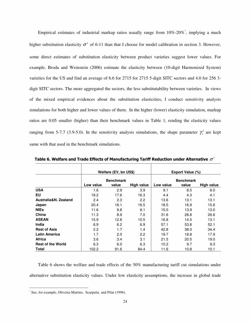
Empirical estimates of industrial markup ratios usually range from 10%-20%7, implying a much

higher substitution elasticity sσ of 6-11 than that I choose for model calibration in section 3. However,

some direct estimates of substitution elasticity between product varieties suggest lower values. For

example, Broda and Weinstein (2006) estimate the elasticity between (10-digit Harmonized System)

varieties for the US and find an average of 6.6 for 2715 for 2715 5-digit SITC sectors and 4.0 for 256 3-

digit SITC sectors. The more aggregated the sectors, the less substitutability between varieties. In views

of the mixed empirical evidences about the substitution elasticities, I conduct sensitivity analysis

simulations for both higher and lower values of them. In the higher (lower) elasticity simulation, markup

ratios are 0.05 smaller (higher) than their benchmark values in Table 1, rending the elasticity values

ranging from 5-7.7 (3.9-5.0). In the sensitivity analysis simulations, the shape parameter s

iγ are kept

same with that used in the benchmark simulations.

Table 6. Welfare and Trade Effects of Manufacturing Tariff Reduction under Alternative sσ

Welfare (EV, bn US$) Export Value (%)

Low value Benchmark

value High value Low value Benchmark

value High value

USA 1.6 2.9 3.9 9.1 8.5 8.0

EU 18.2 17.6 16.3 4.4 4.3 4.1

Australia&N. Zealand 2.4 2.3 2.2 13.6 13.1 13.1

Japan 20.4 18.1 16.5 18.5 16.9 15.6

NIEs 11.6 9.8 8.1 15.0 13.9 13.0

China 11.3 8.9 7.0 31.6 28.8 26.6

ASEAN 15.9 12.8 10.5 16.8 14.5 13.1

India 6.9 6.2 6.9 57.1 53.8 52.1

Rest of Asia 2.2 1.7 1.4 42.8 38.0 34.4

Latin America 1.7 2.0 2.2 19.7 18.8 17.9

Africa 3.6 3.4 3.1 21.5 20.5 19.0

Rest of the World 6.3 6.0 6.3 10.2 9.7 9.3

Total 102.2 91.6 84.4 11.6 10.8 10.1

Table 6 shows the welfare and trade effects of the 50% manufacturing tariff cut simulations under

alternative substitution elasticity values. Under low elasticity assumptions, the increase in global trade

7 See, for example, Oliveira-Martins, Scarpetta and Pilat (1996).

25

and welfare would be 7%-11% higher than that obtained from benchmark assumptions of substitution

elasticity, while under high elasticities, the global gains in trade and welfare are 6-8% smaller. This is

consistent with the theoretic prediction that the substitution elasticity between varieties has a negative

effect on the elasticity of trade flows with respect to tariff (see equation (32)), as a higher substitution

elasticity makes the extensive margin less sensitive to changes in trade costs, damping the impacts of

tariff on trade flows (Chaney, 2006). This property makes the firm heterogeneity CGE model distinctly

different from Armington CGE model, in which an increase in Armington elasticity roughly causes the

same magnitude of increase in the trade expansion and welfare.

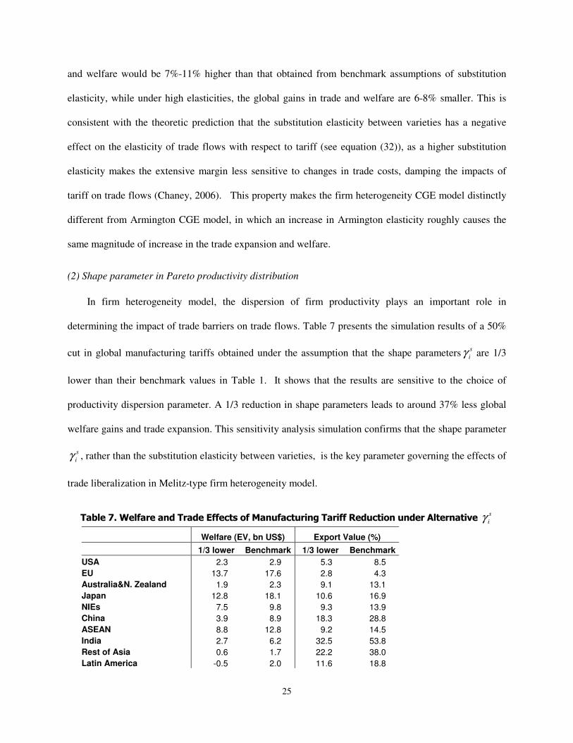
(2) Shape parameter in Pareto productivity distribution

In firm heterogeneity model, the dispersion of firm productivity plays an important role in

determining the impact of trade barriers on trade flows. Table 7 presents the simulation results of a 50%

cut in global manufacturing tariffs obtained under the assumption that the shape parameterss

iγ are 1/3

lower than their benchmark values in Table 1. It shows that the results are sensitive to the choice of

productivity dispersion parameter. A 1/3 reduction in shape parameters leads to around 37% less global

welfare gains and trade expansion. This sensitivity analysis simulation confirms that the shape parameter

s

iγ , rather than the substitution elasticity between varieties, is the key parameter governing the effects of

trade liberalization in Melitz-type firm heterogeneity model.

Table 7. Welfare and Trade Effects of Manufacturing Tariff Reduction under Alternative s

iγ

Welfare (EV, bn US$) Export Value (%)

1/3 lower Benchmark 1/3 lower Benchmark

USA 2.3 2.9 5.3 8.5

EU 13.7 17.6 2.8 4.3

Australia&N. Zealand 1.9 2.3 9.1 13.1

Japan 12.8 18.1 10.6 16.9

NIEs 7.5 9.8 9.3 13.9

China 3.9 8.9 18.3 28.8

ASEAN 8.8 12.8 9.2 14.5

India 2.7 6.2 32.5 53.8

Rest of Asia 0.6 1.7 22.2 38.0

Latin America -0.5 2.0 11.6 18.8

26

Africa 1.2 3.4 12.8 20.5

Rest of the World 3.0 6.0 6.2 9.7

Total 57.8 91.6 6.8 10.8

(3)Fixed trade costs

The base year numbers of exporting firms and variable and fixed trade costs are calibrated based on

the assumption of unity elasticity of trade flows with respect to the share of exporting firms. To explore

the sensitivity of model results to the size of fixed trade costs, I assign a higher elasticity of trade flows

with respect to the share of exporting firms in model calibration. This higher elasticity results that on

average the base year numbers of exporting firms are 30% smaller than the benchmark values and the

fixed trade costs are 180% higher. Table 8 reported the welfare effects of the three trade liberalization

simulations under the new assumption about fixed trade costs. It shows that the results are essentially

unchanged for the three simulations. This is not surprising because the policy shocks imposed in the three

simulations are all expressed as percentage changes relative to their baseline levels.

Table 8. Welfare Effects of Trade Liberalization under Higher Fixed Trade Costs (EV, bn US$)

Tariff Cut Variables trade costs

reduction Fixed trade costs

reduction

Higher Fixed Costs Benchmark

Higher Fixed Costs Benchmark

Higher Fixed Costs Benchmark

USA 2.9 2.9 32.9 32.9 64.8 64.9

EU 17.6 17.6 134.7 134.7 205.1 203.9

Australia&N. Zealand 2.3 2.3 5.3 5.3 8.7 8.7

Japan 18.1 18.1 13.3 13.3 24.0 24.2

NIEs 9.8 9.8 23.6 23.6 39.0 39.1

China 9.0 8.9 22.4 22.4 36.1 36.1

ASEAN 12.8 12.8 36.0 35.9 50.8 50.6

India 6.2 6.2 4.8 4.8 7.3 7.4

Rest of Asia 1.7 1.7 2.8 2.8 4.3 4.3

Latin America 2.0 2.0 30.3 30.3 53.7 53.5

Africa 3.4 3.4 10.9 10.9 17.3 17.3

Rest of the World 6.1 6.0 39.0 39.0 66.0 66.0

Total 91.8 91.6 356.0 356.0 577.3 576.0

27

6. Conclusions

The recent models of international trade with heterogeneous firms have opened up a new way for

empirical CGE models to better understand the effects of trade liberalization. This paper builds a multi-

region, multi-sector global CGE model with firm heterogeneity, monopolistic competition and fixed trade

costs a la Melitz(2003) and calibrates it to GTAP database. Some illustrative trade liberalization

simulations using it demonstrate that introducing firm heterogeneity improves the ability of CGE model

to capture the trade expansion and welfare effects of trade liberalization. However, the model results are

sensitive to the shape parameters of firm productivity distribution. Future efforts need to be devoted to

get better estimates for the degree of firm heterogeneity.

28

References

Abler, David, 2006. "Approaches to Measuring the Effects of Trade Agreements CATPRN," mimeo,

Department of Agricultural Economics and Rural Sociology, Pennsylvania State University

Armington, Paul S, 1969. "A Theory of Demand for Products Distinguished by Place of Production. "

IMF Staff Paper, 16(1):159-178.

Bergoeing, Raphael and Timothy J. Kehoe, 2001. "Trade theory and trade facts," Staff Report 284,

Federal Reserve Bank of Minneapolis

Bernard, Andrew, J. Bradford Jensen, and Peter Schott, 2006. "Trade Costs, Firms and Productivity."

Journal of Monetary Economics, 53(5), 917-937

Bernard, Andrew, Jonathan Eaton, J. Bradford Jensen, and Samuel Kortum, 2003. "Plants and

Productivity in International Trade," American Economic Review 93(4), 1268-1290

Broda, Christian and David E. Weinstein, 2006. "Globalization and the Gains from Variety," Quarterly

Journal of Economics, MIT Press, vol. 121(2), pages 541-585, May

Brown, Drusilla K. 1987. "Tariffs, the Terms of Trade, and National Product Differentiation," Journal of

Policy Modeling, 9(3):503-26.

Chaney, Thomas, 2006. "Distorted Gravity: Heterogeneous Firms, Market Structure, and the Geography

of International Trade," mimeo, University of Chicago

Debaere, Peter and Mostashari, Shalah, 2005. "Do Tariffs Matter for the Extensive Margin of

International Trade? An Empirical Analysis," CEPR Discussion Papers 5260

Del Gatto, Massimo, Giordano Mion, and Gianmarco I.P. Ottaviano, 2006. "Trade Integration, Firm

Selection and the Costs of Non-Europe" (June 2006). CEPR Discussion Paper No. 5730

de Melo, Jaime, and Sherman Robinson. 1992. “Productivity and Externalities: Models of Export-Led

Growth.” The Journal of International Trade and Economic Development, Vol. 1, No. 1, 41-68.

Devarajan, Shantayanan and Sherman Robinson, 2005. “The Influence of Computable General

Equilibrium Models on Policy.” in Frontiers in Applied General Equilibrium Modeling: In Honor of

Herbert Scarf, ed. T.J. Kehoe, T.N. Srinivasan, and J. Whalley, pp. 341-377. Cambridge, UK:

Cambridge University

Eaton, Jonathan, Samuel Kortum, and Francis Kramarz, 2004. "Dissecting Trade: Firms, Industries, and

Export Destinations," American Economic Review, Vol. 94(2), pages 150-154, May

29

Falvey, Rod, David Greenaway, and Zhihong Yu, 2006. "Extending the Melitz Model to Asymmetric

Countries." University of Nottingham Research Paper No. 2006/07

Helpman, Elhanan, Marc Melitz, and Stephen Yeaple, 2004. "Export Versus FDI with Het-erogeneous

Firms," American Economic Review, 94(1) 300-316

Hummels, David and Peter J. Klenow, 2005. "The Variety and Quality of a Nation's Exports," American

Economic Review, 95(3), 704-723

Kehoe, Timothy J. 2005. "An Evaluation of the Performance of Applied General Equilibrium Models on

the Impact of NAFTA. " in Frontiers in Applied General Equilibrium Modeling: In Honor of

Herbert Scarf, ed. T.J. Kehoe, T.N. Srinivasan, and J. Whalley, pp. 341-377. Cambridge, UK:

Cambridge University

Kehoe, Timothy J. and Kim J. Ruhl, 2003. "How Important Is the New Goods Margin in International

Trade?," Staff Report 324, Federal Reserve Bank of Minneapolis.

Krugman, Paul, 1979. "Increasing Returns, Monopolistic Competition and International Trade, " Journal

of International Economics, 9, 469-479

Kuiper, Marijke, and Frank van Tongeren, 2006. "Using Gravity to Move Armington - An Empirical

Approach to the Small Initial Trade Share Problem in General Equilibrium Models." Presented at the

9th Annual Conference on Global Economic Analysis, Addis Ababa, Ethiopia

Lewis, Jeffrey D., Sherman Robinson, and Zhi Wang, 1995, "Beyond the Uruguay Round: The

Implication of an Asian Free Trade Area." China Economic Review 7: 35-90

Melitz, Marc J. 2003. "The Impact of Trade on Intra-Industry Reallocations and Aggregate Industry

Productivity," Econometrica, 71(6), 1695-1725

Melitz, Marc J., and Gianmarco I.P. Ottaviano, 2005. "Market Size, Trade, and Productivity," NBER

Working Paper No. 11393

Oliveira Martins, Joaquim, Stefano Scarpetta, and Dirk Pilat, 1996. "Mark-Up Ratios in Manufacturing

Industries: Estimates for 14 OECD Countries," OECD Economics Department Working Papers 162,

OECD Economics Department

Yeaple, Stephen Ross, 2005. "A Simple Model of Firm Heterogeneity, International Trade, and Wages,"

Journal of International Economics, 65(1), 1-20

Yi, Kei-Mu, 2003. "Can Vertical Specialization Explain the Growth of World Trade?," Journal of

Political Economy, Vol. 111(1):52-102, February

30

World Bank, 2001. Global Economic Prospects, 2002: Making Trade Work for the World's Poor,

Washington D.C.: World Bank.