1

“Assessing classification methods for churn prediction by composite

indicators”

M. Clemente*, V. Giner-Bosch, S. San Matías

Department of Applied Statistics, Operations Research and Quality, Universitat Politècnica de

València, Camino de Vera s/n, 46022 Spain.

*Corresponding author. Tel.: +34 96 387 74 90; Fax: +34 96 387 74 99.

Email addresses: mclement@eio.upv.es (M. Clemente), ssanmat@eio.upv.es (S.San Matías), vigibos@eio.upv.es (V. Giner-Bosch)

Keywords: Churn prediction, Composite indicators, Classification, Data mining.

Abstract

Customer churn prediction is one of the problems that most concern to businesses today.

Predictive models can be developed for identifying future churners. As the number of suitable

classification methods increases, it has become more difficult to assess which one is the most

effective for our application and which parameters to use for its validation. To select the most

appropriate method, other aspects apart from accuracy—which is the most common

parameter— can and should be considered as for example: robustness, speed, interpretability

and ease of use. In this paper we propose a methodology for evaluating statistical models for

classification with the use of a composite indicator. This composite indicator measures

multidimensional concepts which cannot be captured by a single parameter and help decision

makers to solve this complex problem. Three alternatives are proposed giving different

weights to the involved parameters considering the final user priorities. Our methodology

finds which the best classifier is by maximizing the value of the composite indicator. We test

our proposal on a set of five churn classification models drawn from a real experience, three of

them being based on individual classifiers (logistic regression, decision trees and neural

2

networks), and the other two being constructed by using combined classifiers (AdaBoost and

Random forest).

Another added value offered by this work is to consider the input variables selection influence

on the performance of the churn prediction model. We will consider four different

alternatives: original variables, aggregate variables (together with original ones), Principal

component analysis (PCA) and stacking procedure.

Numerical results using real data from a Spanish retailing company are presented and

discussed in order to show the performance and validity of our proposal.

1. INTRODUCTION

1.1 Customer churn prediction

Customer retention is one of the fundamental aspects of Customer Relationship Management

(CRM), especially within the current economic environment, since it is more profitable to keep

existing customers than attract new one [2,12,29]. A small improvement in customer retention

can produce an increase in profit [30].

The early detection of future churners is one of the CRM strategies. Predictive models provide

us with a numerical measure that assigns to each client their propensity to churn in terms of

probability. The higher the propensity value assigned to a customer, the greater their

inclination to leave the firm. This information can be used by the company to develop

marketing campaigns aimed at customer retention.

To build such predictive models, several statistical strategies for classification (such as logistic

regression, neuronal network, etc.) can be used.

After being built, predictive models have to be validated, and this can be done in terms of

different criteria, for instance: accuracy, speed, robustness, interpretability and ease of use. It

is common to develop several models using different statistical strategies to compare them

and select the most appropriate classification system for a specific problem.

3

Verbeke et al. [32] provide an overview of the literature on the use of data mining techniques

for customer churn prediction modeling. They show the characteristics of the assessed

datasets, the different applied modeling techniques and the validation and evaluation of the

results. Different evaluation parameters are used in the considered studies, most of them

being mainly based on aspects related to the accuracy of the model. The metrics that were

more frequently used are percentage of correctly classified (PCC), area under curve (AUC), Top-

decile and lift.

Regarding classification techniques, some authors focus at individual classifiers, such as logistic

regression, neural networks and classification trees. Moreover, thanks to the improvement in

computer hardware, other techniques have been recently developed as a combination of

other individual classifiers. Some examples of these techniques are Random forest (based on

bagging) and AdaBoost (based on boosting).

Despite of this diversity, we didn’t find works which evaluated the accuracy against other

parameters such as speed, robustness, interpretability and ease of use. Those other

parameters are also important, as a classification model has not only to be accurate but also

interpretable, usable and implementable by final users.

In fact, some authors (see for example Buckinx et al.[9]) conclude that different predictive

techniques happened to show similar accuracy levels on their data, so other discriminant

parameters could be used. Buckinx et al. [9] work on real data from a retail company. They use

logistic regression, neural networks and random forest as classification techniques and the

performance is assessed through the percentage of correctly classified and the AUC.

Besides the standard measures of accuracy, we find the results of a study on a financial

services company in Belgium performed by Glady et al. [18]. In this case, a framework is

provided for evaluating churner classification techniques based on the profit loss incurred by a

misclassification, considered from a customer lifetime value perspective. At the same way,

Verbeke et al. [31] propose a profit centric performance measure. They use the idea of

4

maximum profit to evaluate customer churn prediction models in the telecommunication

sector. Comprehensibility and interpretability of churn predictive models has recently gained

some more attention. We find some examples at [24] or [32].

As a summary, an overview of the present literature on churn predictive models shows that

most of the papers focus on the accuracy of models and they pay little attention to other

parameters, although it is now generally recognized that there are other important dimensions

to be considered when assessing the performance. Even if a model is accurate, it cannot be

said to be of good quality if it spends too much time for processing data or if it is not easily

interpretable. Thus, quality is a multi-faceted concept. The most important characteristics

depend on user perspectives, needs and priorities, which may vary across user-groups.

Therefore, we propose a methodology aiming at providing easier and better decisions when

choosing among different classification methods, in the context of churn prediction, not only

relying on the accuracy of the methods but also in their interaction with other important

parameters such as: robustness, speed, interpretability and ease of use. We will do this by

joining all these parameters in a composite indicator.

The use of composite indicators is not very usual at assessing classification methods for churn

prediction, but it is very common in other areas. For example, Composite indicators (CIs) which

compare country performance are increasingly recognized as a useful tool in policy analysis

and public communication. In a recent review of this matter, Bandura [3] cites more than 160

composite indicators for providing simple comparisons of countries used by various

organizations around the world to compare elusive issues in wide-ranging fields, e.g.,

environment, economy, society or technological development.

As a second objective, we will also study the effect of the selection of input variables on the

performance of the churn prediction model. More precisely, we will consider four different

alternatives: original variables, aggregate variables (together with original ones), Principal

component analysis (PCA) and stacking procedure.

5

Our paper is organized as follows: in section 2 we further discuss the different criteria than can

be used in order to assess a classification method. In section 3 we make a description of the

statistical classification techniques that are most commonly used in churn prediction. In

section 4 we describe the methodology we have developed. First we detail the different ways

we have considered for selecting input variables and also how classification techniques have

been tuned; second we define a composite indicator for assessing churn predictive models.

Then, in the section 5 we present and discuss the results obtained when applying our proposal

to a real dataset and finally, the conclusions of the study and future steps are stated.

2. EVALUATION OF CLASSIFICATION MODELS

Classification model can be evaluated according to different criteria as mentioned above.

Accuracy is the most common evaluation parameter, but we don’t have to look out the other

parameters. This section provides a non-exhaustive summary of the general characteristics of

these parameters.

2.1 Accuracy

Predictive models provide us with a numerical measure that assigns to each client their

propensity to churn in terms of probability. We can turn this probabilistic classifier into a

binary one using a certain threshold to determine a limit between classes.

The accuracy of a model is an indicator of its ability to predict the target class for future

observations. The most basic indicator is the proportion of observations of the test set

correctly classified by the model. Similarly, the error rate is calculated as the ratio between the

number of errors and the number of cases examined.

It is not only important to measure the number of cases correctly or incorrectly classified, but

also the type of error made. In churn prediction, it is normal that the churn rate is much lower

than the retention rate in the company - that is called a class imbalance problem [34]. In this

6

context, it is more appropriate to use decision tables; usually called confusion matrices (see

[33] for a more detailed explanation).

2.1.1. Confusion matrix

Be a binary classification problem with two possible classes: + and - (Positive and negative).

The confusion matrix is a contingency table of 2X2 whose rows correspond to the observed

values and the predicted values by the classification model are shown at the columns, as we

can see in Table 1.

Predictions

Observations - (negative) + (positive) Total

- (negative) p q p + q

+ (positive) u v u + v

Total p + u q + v m

Table 1. The confusion matrix for a binary classification problem

To assess the classification results we count the number of the correct predictions for the

negative examples (p); the number of incorrect predictions for the positive examples (u); the

number of the incorrect predictions for the negative examples (q); the number of correct

predictions for the positive examples (v). From the cell counts contained in the confusion

matrix a number of ratios that serve to validate the classification algorithm can be calculated.

• Overall accuracy measures the percentage of correct classified (PCC)

��� =� + �

�

• Sensitivity, also known as true positive rate, measures the proportion of positive

examples which are predicted to be positive. In our case, sensitivity means the

percentage of correctly classified in class "Churn".

�������� = �

� + �

7

• Specificity, also known as true negative rate, measures the proportion of negative

examples which are predicted to be negative. In our case, specificity means the

percentage of correctly classified in class "Non-Churn".

��������� = �

� + �

As we previously mentioned, the threshold of a probabilistic classifier could be varied in order

to assign the instances to the target class. So, the sensitivity, specificity and PCC vary together

in function of the specific cut off.

2.1.2 Receiver Operating Characteristic curve

A Receiver Operating Characteristic (ROC) chart is a two-dimensional plot with the proportion

of false positives (1- specificity) on the horizontal axis and the proportion of true positives on

the vertical axis (sensitivity) when using different cut-off for a classifier score. Each point on

the ROC curve represents a sensitivity/specificity pair corresponding to a particular decision

threshold. The optimal balance point between sensitivity and specificity can be determined

using this graph. On the other hand, the ROC analysis allows us to assess the predictive ability

of a classifier independent of any threshold. A common measure for comparing the accuracy of

various classifiers is the area under the ROC curve (called AUC). It evaluates the method's

ability to correctly classify. The classifier with the greatest AUC will be considered better. The

closer to 1 is the AUC of a classifier, the higher accuracy.

In our context, the AUC can be interpreted intuitively as the probability that at a couple of

clients, one loyal and one that churns, the method correctly classify both of them.

2.2 Speed

The computing time for obtaining a model with a specific classification method is determined

in terms of different aspects: classification method used, computer specification and data set

size.

Some methods take longer to run than others, mainly for the type of classification procedure.

It is important to consider the system requirements for each method, like specific hardware

8

platform or operating system. These requirements for a particular application could be critical

to many companies, because it has already a computer platform. When the method takes a

long time, sometimes it is applied over a smaller training sample and the results are applied to

the rest.

In conclusion, we define speed as the time spent to obtain a model from a train dataset, for a

given hardware and a specific sample size.

2.3 Robustness

A classification method is said to be robust when its accuracy remains quite stable regardless

of the dataset it is being applied on. More precisely, robustness can be defined as the

difference of accuracy between training and test datasets.

Other aspects that also concern robustness are the ability of the method to deal with the

presence of missing data and outliers.

2.4 Interpretability

The purpose of classification analysis is interpreting as well as predicting, so the classifying

rules provided by models should be simple and easy to understand by end users.

In the case of churn prediction, models are expected to help the company to design better

retention campaigns. In order to achieve that, the rules given by the model have to be easily

translatable into greater knowledge about the profile of customer who churns.

In the case of the interpretability, it is generally recognized that there are some methods more

interpretable than others, we order the different predictive techniques in terms of relative

positions (use of ranking) and after we assign a score.

2.5 Ease of use: accessibility

Currently, we can find a great variety of software at the marketplace. However, there are

certain aspects that will condition our decision as the tool’s suitability to the intended users.

We are referring specifically a user friendly and open source software.

9

The open source software permits the unlimited tuning and improvement of a software

product by the user and large communities and to adapt it to changing conditions. However, it

is needed more education for a regular user before he can profit the versatility of open source

software. Other advantage is that this software is available without fee.

On another hand, an easy data load and manipulation or window environment could be very

important for a non-expert user. It is easier to find these characteristics in commercial

statistical software than in open source software.

In conclusion, the ease of use is a qualitative measure which depends on the specific user

characteristics. In this work, we will assign a value considering our circumstances as we will

explain later in the methodology section.

3. DESCRIPTION OF CLASSIFIERS

As we have previously mentioned, churn prediction can be dealt with by using different

classification statistical and data mining techniques. In this section we describe and revise the

most frequently used techniques for this task, which we have actually used in this study.

3.1 Individual Classifiers: Logistic Regression, Decision Trees and Neural Networks

Logistic regression, decision tree and neural networks are well-known data mining algorithms.

The study conducted by Neslin [27] shows that these three classifying methods are some of

the most frequently used estimation techniques in the field of churn prediction. They are

actually considered also as a reference to compare with when testing other more sophisticated

techniques [9,18].

The purpose of regression models is to identify a functional relationship between one variable,

called the dependent variable or the response, and others, called independent variables or

explanatory variables. When dealing with qualitative response variable logistic regression can

be used. A qualitative response problem can often be decomposed into binary response

problems. Logistic regression is a technique for converting binary classification problems into

10

linear regression ones, by means of a proper transformation. It is a standard statistical method

used in many different contexts [33].

Tree models produce a classification of observations into groups and then obtain a score for

each group. One of the most used tree algorithms in the statistical community is the CART

(Classification and Regression Trees) algorithm. The purpose of CART analysis is to predict or

classify cases according to a response variable. CART uses a binary recursive partitioning

method that produces a decision tree. The tree is structured as a sequence of simple (split)

questions based on several predictor variables, and (in our context) identifies subgroups of

customer at higher likelihood of defect (see [8] for more information on CART).

Artificial Neural Networks try to imitate the properties of biological neurons. Although they

can be used for many purposes (e.g. descriptive data mining), we explore its predictive use.

The multilayer perceptron is the most used architecture for predictive data mining. In it, input

variables are organized in one layer of neurons that is connected with successive layers, the

last of them being the output or response layer. Connection weights, bias terms or neurons,

and activation functions are used to combine values (neurons) in each layer and to obtain

values that are considered as inputs for the next layer. Multilayer perceptron can be

considered as a non-linear predictive model [5].

3.2 Ensemble Classification: Random Forest, Adaboost and Stacking

The strategy of combining predictions from multiple classifiers to produce a single final

classifier has been a popular field of research in recent years that is known as ensemble

classification. Several studies have demonstrated that the resulting ensemble can produce

better results than any of the individual classifiers making up the ensemble [4,15].

Some of the most popular methods for creating accurate ensembles are Bagging [7] and

Boosting [17].

In Bagging (Bootstrapping and Aggregating), the results of each of the classifiers obtained from

the same training set (using bootstrap) are aggregated through majority vote. In other words,

11

instances are classified as the class that is most frequently assigned by the ensemble members.

Breiman [6] developed a new ensemble algorithm based in bagging, called Random Forest, in

which decision trees are used as base classifier. Unlike Bagging, in Boosting the resampling of

the training set is dependent on the performance of the earlier classifiers, as the classifiers are

built sequentially using previous performances. The most well-known boosting algorithm is

AdaBoost (Adaptative Boosting) [17]. In AdaBoost, instances that are incorrectly predicted

receive higher weight during consecutive training iterations and therefore, new classifiers are

produced to improve the current poor ensemble's performance.

Random forests have been used for customer retention modeling [21] and churn prediction

[9,13], also with variations of the original model such as weighted random forests [10].

The application of AdaBoost in customer churn prediction is very popular too. We find some

examples in [14,20,22]. In Glady [18], a version of AdaBoost algorithm is implemented, the

AdaCost. It belongs to the class of Cost-Sensitive Classiffiers.

The ensemble learning method called Stacking is a little bit different from the methods we

have just described. The stacking algorithm [35] follows a meta-classification scheme. The idea

behind stacking is to use the predictions from the original classifiers as attributes in a new

training set that keeps the original class labels. Essentially, Stacking combines output from a

set of several base classifiers via one meta classifier. In our case, the class is the output and the

each classifier predictions are the inputs.

We used Stacking with the following base classifiers: Logistic Regression, Decision Trees and

Neural Networks logistic regression, which were chosen in an attempt to compare with our

own results with individual classifiers.

In our work, we consider the stacking as an input variable characteristic instead of a

classification method as we will explain later.

4. METHODOLOGY

12

On the following sections, firstly we are going to describe the input variable selection

procedure, and after that how to calculate the “Evaluation Composite Indicator”.

4.1 Input variable selection

Our main aim is to study the performance of a churn prediction model based on different

parameters included in an only composite indicator. However, we are also interested on study

the impact of the input variable in this performance and whether we should make or not

reduction of variables to implement the classification techniques.

It is usually to apply a data reduction technique in order to obtain a model more efficient,

without sacrificing the information quality of the original dataset.

Some authors prefer a limited number of highly predictive variables, in order to improve the

comprehensibility of classification models, even at the cost of a somewhat decreased

discrimination power [25,28].

In Verbeke et al. [31], a generic variable input selection procedure is applied which iteratively

reduces the number of variables included in the model. They find an optimal trade-off

between minimizing the number of variables and maximizing the discriminatory power.

In our case, the available data consists on demographic information on each customer and the

transactions carried out for purchasing and using services. In order to obtain a quality dataset,

we had previously performed some process such as cleaning, processing and data selection.

Any variable having too many missing or invalid values were eliminated from the analysis.

From the original variables other aggregate variables were calculated (linear and nonlinear

transformations).

Four options were defined in order to more efficiently determine the set of predictor variables.

In the first option only the original numerical variables and categorical variables are used. We

will denote it as OP1-OV. That is, we do not consider the aggregate variables, many of which

have nonlinear characteristics respect to the original data. Depending on the methods of

classification, there are some which are better than others to get the nonlinear relationship

13

between the explanatory variables and the dependent variable. We want to assess whether

the use of only original variables penalizes or not the results. In the second group we used as

explanatory variables all the original numerical variables, categorical variables and aggregate

variables. We will denote it as OP2-AV.

The number of variables is very high, in both options 1 and 2. Some classification methods are

not operating with such a large number of variables along with a number of records also high.

In these cases, we apply an algorithm to reduce the number of variables. This procedure is

summarized in Algorithm 1.

Algorithm 1 – Variables number reduction

Step 1. Consider the classification method CM.

Step 2. Divide the total number of variables in k groups called primary blocks.

Step 3. Train a model for predicting the class "churn" with the method CM, on the training

sample and using variables of the primary block j, for each j = 1. . . k.

Step 4. Define a secondary block composes by the most important variables of each block,

depending on the models trained in step 3.

Step 5. Train a final model to predict the class "churn" with the CM model on the training

sample and using the secondary block variables.

In order to reduce the computing time, we tried a third option. In this case, we conducted a

principal components analysis (PCA) over the total number of variables (original and

aggregates). That way, the number of explanatory variables was reduced in a number of lower

factors. We will denote it as OP3-PCA.

At the fourth option, we use the stacking method. As mentioned above, it uses a classification

method for combining the results of all basic classifiers. In this method, the inputs are the

predictions of each classifier and the output is the predicted class. We will denote it as OP4-SV.

The explanatory variables of Option 4 are:

14

• Propensities (predicted probabilities) obtained by each of the classifiers used in the

options 1, 2 and 3.

• Propensities obtained with the primary blocks of options 1 and 2. These propensities

are obtained when applying the algorithm 1 “Variables number reduction”.

4.2 Evaluation Composite Indicator (ECI)

In general terms, an indicator is a quantitative or a qualitative measure derived from a series

of observed parameters. Usually, it seems easier to interpret composite indicators than

identify common trends across many separate indicators with wide-ranging fields. Our aim is

to measure multidimensional concepts which cannot be captured by a single parameter and

facilitate communication with general public [26].

We have created an indicator that includes the effects of the different parameters used to

evaluate the performance of a churn prediction. We will call Evaluation Composite Indicator

(ECI).

First of all, we have to distinguish between the quantitative and qualitative parameter. The

accuracy, speed and robustness are a quantitative measure, so they are easily quantifiable.

However, the interpretability and the ease of use are difficult to measure, because it is a

subjective measure. In the case of the interpretability, it is generally recognized that there are

some methods more interpretable than others. We assign a score for each method (as we will

explain later), so we transform it in a quantitative parameter.

However, the ease of use depends on the specific user characteristics. For this reason, we do

not include this parameter at the ECI, although we take it into consideration.

4.2.1 ECI Parameters

To analyze the accuracy of predictive techniques, we will focus primarily on the results

obtained for the test set, which are the cases that have not been used for model estimation.

The parameter we have considered to assess the accuracy and predictive ability of the

15

classification techniques used are the AUC (area under the ROC curve). We denote this

parameter as “A”.

The running time on the test set (measure in minutes) has helped us to evaluate the speed and

scalability. The scalability of a classifier is connected with the ability to learn from large

databases, and thus also relates to the execution time. We denote this parameter as “S”.

Regarding robustness (“R”), the issue of missing data and outliers is already solved in the

database we are handling. Another thing to check is that the differences between the results

of the AUC obtained for the training and test group are not too large. We measure this value

as: Robustness= (AUC_test - AUC_train)

For quantifying the interpretability, we use a ranking for ordering the different predictive

techniques. In our case, we have four relative positions where the best case has a score of 4

points and the worst case a score of 1 point. The four relative positions are “high

interpretability”, “medium interpretability”, “poor interpretability” and “null interpretability”.

In the case of ease of use, we consider two aspects: user friendly and open source software.

The final parameter, denoted as “E”, is obtained by the sum of this two things and it has to be

adapted depending on user needs and priorities.

4.2.2 ECI definition

The indicators should be normalized to render them comparable, because they have different

measurement units. A different types of normalization methods exist [16,19] , but we have

chosen two of the most popular: Standardisation (or z-scores) and Min-Max.

Standardisation (or z-scores) converts indicators to a common scale with a mean of zero and

standard deviation of one. The Min-Max normalises indicators to have an identical range [0, 1]

by subtracting the minimum value and dividing by the range of the indicator values.

The following notation is employed throughout the article:

Xq : raw value of individual indicator q, with q=A (accuracy),S (speed), R(robustness),

I(interpretability) and E(ease of use).

16

Nq,c : normalized value of individual indicator q for normalized method c, with c=Z (z-scores) or

MM (Min-Max).

ECIc _k: value of the composite indicator for normalized method c and k denotes the different

weighting alternatives tested, with k=1,2…K

The simplest additive aggregation method entails the calculation of the value according to

each individual parameter and summation of the resulting indicators. However, the most

widespread linear aggregation is the summation of weighted and normalized individual

indicators:

ECI�,� = ∑ w� · N�,���� (1)

With ∑ w� = 1� and 0 ≤ wq ≤ 1, for all q=A,S,R,I and E and c=Z,MM

Weights can have a significant effect on the overall composite indicator, however most

composite indicators rely on equal weighting (EW). In spite of which method is used, weights

are essentially value judgments. The analyst should choose weights based on his expert

opinion, to better reflect company priorities or factors more (or less) influential.

For this reason, we have tested three weighting alternatives, considering our priorities. When

there is insufficient knowledge about the relationships between the different components, we

think the best option is to give the same weight to all the variables. However, in some

circumstances, the accuracy or interpretability could be more important than the other

components. Our aim is implementing a marketing campaign against the churn. If the

predictive model is accurate enough, this means that this group of customers should coincide

practically with the real churners. On the other hand, we have to understand what kind of

people is targeted in the campaign, so an interpretable model should be interesting.

1) All variables are given the same weight rankings:

ECIc-1=0.25·A +0.25·S+0.25·R+0.25·I

2) We reward the accuracy and punish the other components:

17

ECIc-2=0.34·A +0.22·S+0.22·R+0.22·I

3) We reward the accuracy and interpretability and punish the other components:

ECIc-3=0.30·A +0.20·S+0.20·R+0.30·I

Our objective is to maximize the ECI obtained. So, we will compare the ECI obtained in the

different classification methods for each of the alternatives proposed at the input variables

selection. The value of the ECI gives a succinct measurement comparing the benefits of

various classifiers: the classifier associated with the ECI which has the greatest value is then

the preferable.

5. RESULTS

We have used real data from a retail distribution company in order to assess the validity of our

proposed methodology. Subsequent subsections discuss the experimental results.

5.1 Dataset

The dataset is obtained from a real company in the group of commercial distribution in Spain.

It is a benchmark company in the retailing and supermarkets. By the type of industry, the

customer relationship with the company is non-contractual. However, the company has a

loyalty card, which although it is not a purchase card, it is used by the company to offer

customers discounts and / or promotions and providing relevant customer information. The

necessary data for doing this job was extracted from the available information of clients who

used the loyalty card. The time period for the study is composed of the information from June

2006 to November 2007.

Due to the size of the database and computational reasons, the initial database was randomly

selected in a sample of 15000 instances. This sample was divided into a training (50%) and

validation group (50%). In this database we had an indicator on whether the client was a future

churner or not. It is based on the methodology described in the technical report [11].

5.2 Input variables

18

In many researches, the number of purchases (frequency) and the amount of spending

(monetary) are the most typical predictors. However, Buckinx et al. [9] have shown that other

variables could be also very effective predictors as the length of the customer-supplier

relationship, buying behavior across categories, mode of payment or usage of promotions and

brand purchase behavior. An overview of main available variables in this study can be found in

Table 2. From the original variables other aggregate variables were calculated (linear and

nonlinear transformations). For example: the average of the amount of spending or the

amount of spending multiply by the frequency.

Variable Type Variable name Description

Demographics DOB Date of birth of customer

AGE Age (in years) of customer

NMH Number of members in the household

TOWN Town

POCod Postal code

Purchasing

profile DStart Start Date

LoR_year Length of relationship (years)

LoR_month Length of relationship (month)

CC Commercial code of usual shop

CreditCard Mode of payment (credit card YES/NOT)

Transactional

MONETARY_PDO_i

Monetary amount of spending on products on special

offer (i=month in study)

MONETARY_PDP_i

Monetary amount of spending on house brand

products (i=month in study)

MONETARY_i Total monetary amount of spending (i=month in study)

FREQUENCY_i Number of shop visits with purchase (i=month in study)

MONETARY_SEC_X_i

Aggregated relative spending in 17 different sections:

drinks, fruit and vegetables, dairy products, meat, etc.

(X=1…17 and i=month in study)

MONETARY_CAT_Y_i

Aggregated relative spending in 156 different

categories. A section is composed on different

categories (Y=1…156 and i=month in study)

NSEC3M_i

Number of different section with purchase in the last 3

month (i=month in study)

Table 2. Main input variables used in this study

19

From the available dataset, we kept 462 original variables. These variables were used at first

option OP1-OV as input variables. From these original variables, we calculated some other

aggregates. The second option OP2-AV is composed by 584 variables (original and aggregates).

At the third option OP3-PCA, we conducted a PCA over the total variables (original and

aggregates). The 184 selected factors in this analysis explained 80% of the variability from the

total number of variables, with a value of KMO = 0,595.

Finally at the fourth option OP4-SV, the input variables are composed by the predictions of

previous classifiers. It means a total of 17 variables.

From the point of view of classification methods, logistic regression and Random Forest have

computational problems to treat large datasets, both in terms of number of observations and

number of variables. We apply the algorithm of “Variables number reduction” when the input

variable selection is done for OP1-OV and OP2-AV. In the case of logistic regression, the most

important variables of the primary blocks were selected by choosing the significant variables in

this model for a tolerance of 5% (α=0.05). The secondary block is compounded for these

selected variables. In the case of Random Forest, to determine the importance of the

explanatory variables, we calculated the Gini index for each of them. After that, we ordered

from highest to lowest rate and keep the variables with 20% higher index. The secondary block

is compound for these selected variables.

5.3 Experimental setup

Logistic Regression, classification trees and Neuronal Networks results are obtained with SPSS

v18. AdaBoost and Random Forest analysis was performed using the adabag [1] and

randomForest [23] packages in R, an open source statistical package available at http://www.r-

project.org.

Parameter settings for the algorithms are based on default or recommended values. The

growing method used at classification tree is the CART algorithm. The architecture of the

neural network is set in a single hidden layer and the number of nodes in the layer is

20

determined automatically by the program. The minimum number of units in the hidden layer 1

and the maximum is 50.

CART is used as a base classifier for adaboost and Random Forest algorithm. In the case of

Random Forest, two parameters have to be determined by the user: the number of trees to

build and number of variables randomly sampled as candidates in each division. The first

parameter is set at 500 trees. For the second parameter, we follow Breiman’s

recommendation, the square root of the number of input variables. In the case of Adaboost,

the number of iterations to perform is set at 15.

As mentioned before, the stacking methodology follows an approach slightly different. Here,

the particular characteristic is to consider the predictions obtained for the different options of

input variables selection as explanatory variables. However, logistic regression, classification

trees and neural network were used as individual classifiers with the same parameters we

have explained above.

The characteristics of the equipment used are:

• System with 2 Intel Xeon 2.50GHz E5420 to

• 8GB RAM

• Operating System Windows Server 2008 Enterprise SP2 64-bit

As you can see by the features, it is not a desktop computer, but a high performance server.

5.4 Numerical experiences

The results can be analyzed from the point of view of the input selection options and

classification methods. Firstly, we are going to do a discussion about the result of the

individual parameters and after that, we are going to analyze the ECI results.

5.4.1 Individual parameters discussion

The individual parameters results (without normalization) of the various techniques are

depicted in the table 3 for the different input variable selection options: OP1-OV, OP2-AV,

OP3-PCA and OP4-SV. On the table 3, we will denote the input variable selection options as

21

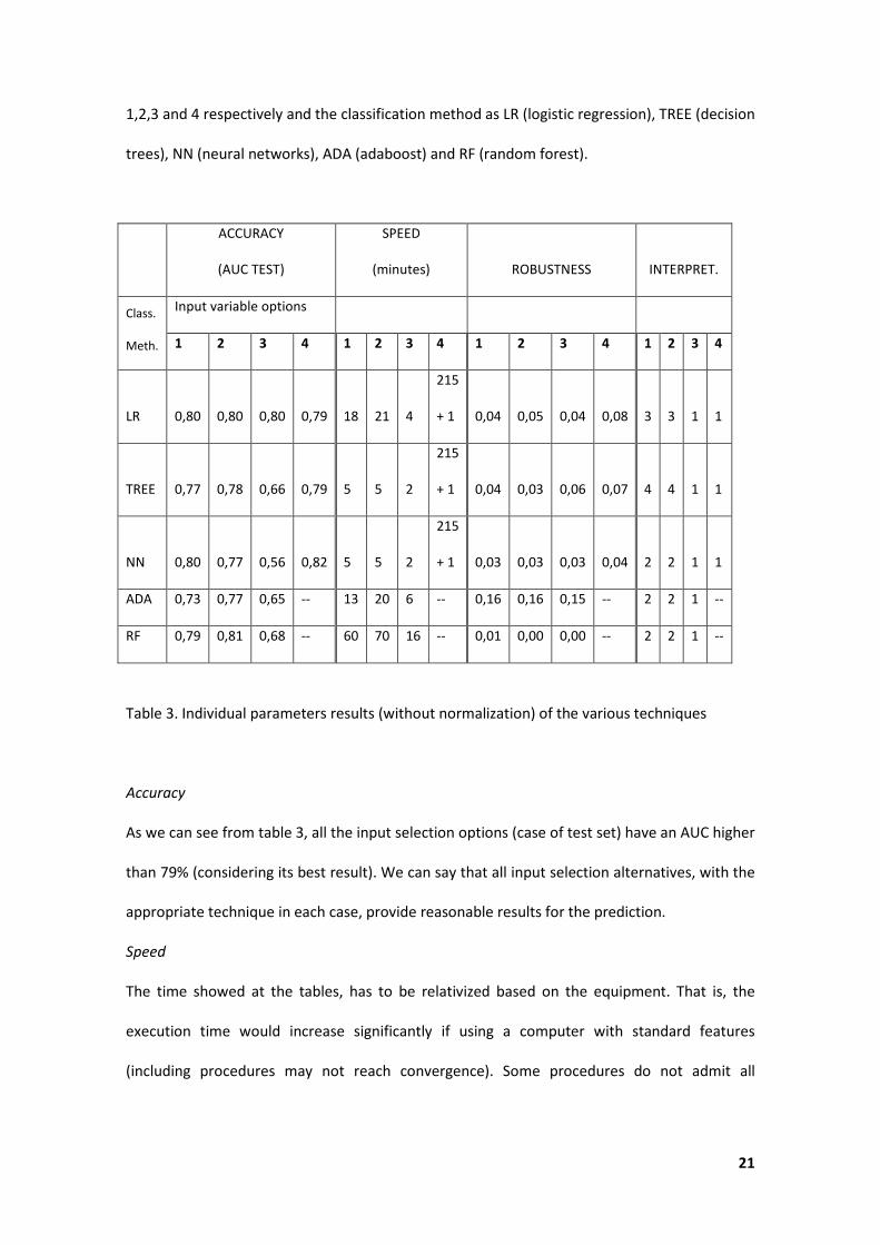
1,2,3 and 4 respectively and the classification method as LR (logistic regression), TREE (decision

trees), NN (neural networks), ADA (adaboost) and RF (random forest).

ACCURACY

(AUC TEST)

SPEED

(minutes) ROBUSTNESS INTERPRET.

Class.

Meth.

Input variable options

1 2 3 4 1 2 3 4 1 2 3 4 1 2 3 4

LR 0,80 0,80 0,80 0,79 18 21 4

215

+ 1 0,04 0,05 0,04 0,08 3 3 1 1

TREE 0,77 0,78 0,66 0,79 5 5 2

215

+ 1 0,04 0,03 0,06 0,07 4 4 1 1

NN 0,80 0,77 0,56 0,82 5 5 2

215

+ 1 0,03 0,03 0,03 0,04 2 2 1 1

ADA 0,73 0,77 0,65 -- 13 20 6 -- 0,16 0,16 0,15 -- 2 2 1 --

RF 0,79 0,81 0,68 -- 60 70 16 -- 0,01 0,00 0,00 -- 2 2 1 --

Table 3. Individual parameters results (without normalization) of the various techniques

Accuracy

As we can see from table 3, all the input selection options (case of test set) have an AUC higher

than 79% (considering its best result). We can say that all input selection alternatives, with the

appropriate technique in each case, provide reasonable results for the prediction.

Speed

The time showed at the tables, has to be relativized based on the equipment. That is, the

execution time would increase significantly if using a computer with standard features

(including procedures may not reach convergence). Some procedures do not admit all

22

variables at once, but note that it was a software problem and not the equipment used. For

these procedures, the execution time is calculated as the sum of each of the split times.

In Option OP4-SV, we distinguished the sum by the total time required to get all the

propensities necessary to carry out the stacking, plus the time required by the final classifier

conducted on these propensities. If we compare the times between options, clearly OP4-SV is

the least efficient, as shown in table 3. Possible improvements in the accuracy obtained with

this method are not worth the time spent in its execution.

We must take into account that for obtaining propensities variables we have to apply a variety

of methods.

If we compare the time used by the different techniques, we note that random forest is the

most expensive. The trees and neural networks methods are the computationally cheapest.

Robustness

From the point of view of input selection options, the robustness of the OP4-SV is lower than

the others when a same classification method is applied. Let us take logistic regression case as

an example. The AUC of the test set worsened between 4.5% and 5.5% with regard to the

training set in options 1 to 3. However, this worsening is 8.7% with the option OP4-SV.

If we make the comparison between techniques, the random forest is clearly the most robust

technique, with deviations close to 0 between the training and validation set.

Interpretability

Regarding individual classifiers, the best known technique is undoubtedly the logistic

regression, but its interpretability is medium. The classification tree is most widely used due to

their conceptual simplicity and the interpretability of the rules they generate. Classification

trees are often quite easy to interpret for the end user. However, neural networks function as

a kind of black box, where from the input data results we obtain a classification, but not a

justification of why this classification is assigned. This makes it more complicated for a non-

expert user.

23

Regarding the combined classifiers, AdaBoost and Random forest, the basic idea is easy to

understand: the winner class is the most voted or the winner is based on a weighted vote.

However, there is not a graphical representation or classification rules easily expressible as in a

classification tree. The results of these methods are more difficult to understand.

On another hand, if we consider the input variables we have an added problem. In the case of

OP3-PCA, the input variables are the factors obtained by applying a Principal Components

Analysis. So, with a 184 factors it is practically impossible to understand the model.

Something similar happens to the option OP4-SV. In this case, the explanatory variables are

the propensities obtained by different methods, so the interpretability is very difficult.

The tree is considered as “high interpretability”, so it should be the first with a score of 4

points. In second place, the logistic regression is considered “medium interpretability” (3

points). The Neuronal network, adaboost and random forest are at the same level, “poor

interpretability” (2 points) . We place at the worst position, the stacking methodology and the

ACP, because they have “null interpretability” due to the type of input variables (1 point).

Ease of use

The individual classifiers we have used are already in most commercial statistical packages and

are easy to handle, because it exists big technical support. Logistic regression, neuronal

network and CART results are obtained using the SPSS software. SPSS is a well-known

commercial tool in the statistic community.

However, the combined classifiers (AdaBoost and Random Forest) are not yet in commercial

statistical packages. The adaboost and Random Forest results were obtained using packages in

R. R is open source software issued under the GNU General Public License. R is a language and

environment for statistical computing and graphics and it is designed around a true computer

language. It allows users to add additional functionality by defining new functions. However, it

is needed more programming education for a regular user before he can profit the versatility

24

of open source software. So, R is more difficult to use for a non-expert user than SPSS

software.

On the other hand, R is open source software and it is available without fee. We consider this

aspect an advantage that we do not find in a commercial statistical package.

In our case, the SPSS software is accessible in our job and we are non-expert programming

user. For our specific circumstances, we consider that the advantages and disadvantages of

both aspects are balanced, so it will not appear on the composite indicator. This consideration

nevertheless cannot be generalized. Some companies or entities for a very wide range of

reasons (economic, political, etc.) have no access to commercial software. On the other hand,

some people do not have sufficient computer skills.

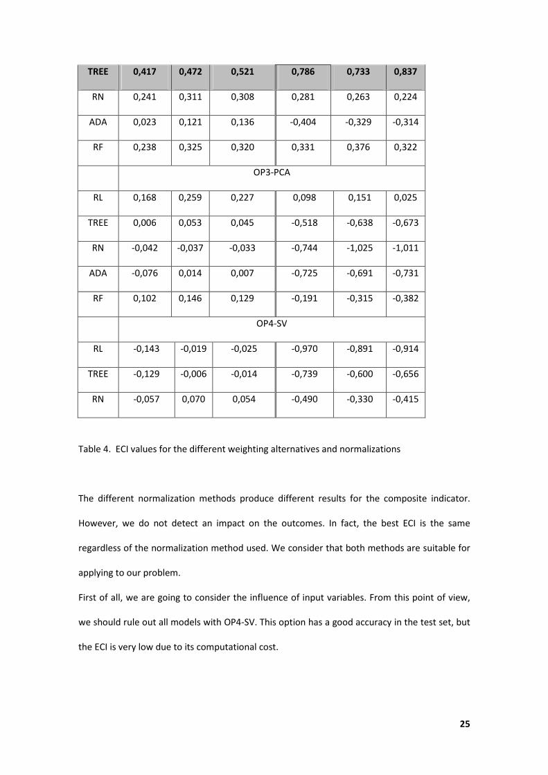
5.4.2 Computation of ECI and discussion

The ECI values for the different weighting alternatives and two normalizations (standardisation

and Min-Max) are shown on the table 4. These values are shown for each option of input

variables selection.

Classif.

Method ECImm-1 ECImm-2 ECImm-3 ECIz-1 ECIz-2 ECIz-3

OP1-OV

RL 0,326 0,402 0,423 0,551 0,565 0,587

TREE 0,383 0,434 0,488 0,667 0,599 0,717

RN 0,269 0,347 0,341 0,388 0,406 0,351

ADA 0,039 0,135 0,149 -0,356 -0,288 -0,277

RF 0,230 0,311 0,308 0,291 0,314 0,268

OP2-AV

RL 0,307 0,384 0,407 0,490 0,507 0,535

25

TREE 0,417 0,472 0,521 0,786 0,733 0,837

RN 0,241 0,311 0,308 0,281 0,263 0,224

ADA 0,023 0,121 0,136 -0,404 -0,329 -0,314

RF 0,238 0,325 0,320 0,331 0,376 0,322

OP3-PCA

RL 0,168 0,259 0,227 0,098 0,151 0,025

TREE 0,006 0,053 0,045 -0,518 -0,638 -0,673

RN -0,042 -0,037 -0,033 -0,744 -1,025 -1,011

ADA -0,076 0,014 0,007 -0,725 -0,691 -0,731

RF 0,102 0,146 0,129 -0,191 -0,315 -0,382

OP4-SV

RL -0,143 -0,019 -0,025 -0,970 -0,891 -0,914

TREE -0,129 -0,006 -0,014 -0,739 -0,600 -0,656

RN -0,057 0,070 0,054 -0,490 -0,330 -0,415

Table 4. ECI values for the different weighting alternatives and normalizations

The different normalization methods produce different results for the composite indicator.

However, we do not detect an impact on the outcomes. In fact, the best ECI is the same

regardless of the normalization method used. We consider that both methods are suitable for

applying to our problem.

First of all, we are going to consider the influence of input variables. From this point of view,

we should rule out all models with OP4-SV. This option has a good accuracy in the test set, but

the ECI is very low due to its computational cost.

26

On the other hand, we discard as well the OP3-PCA, because the ECI is lower than OP1-OV and

OP2-AV. One of the biggest problems of the OP3-PCA is the poor interpretability results and

the low AUC at the test set for some classification methods.

Therefore, it seems quite clear that the optimal selection of explanatory variables is choosing

all the original variables, with aggregate (OP2-AV) or without aggregate variables (OP1-OV).

As a matter of fact, if we selected the input variables according to the maximum ECI, we

should choose the option OP2-AV. However, the difference between the first and second

option is very small. At the first option, we are just using original variables, so it entails less

variables and less computational job. Both alternatives OP1-OV and OP2-AV would be a good

decision.

Considering the OP1-OV and OP2-AV, we can see that the classifier accomplishing the highest

ECI is the classification tree. It achieves the highest value at the three ECI alternatives tested:

equal weights, giving priority to accuracy and giving priority to accuracy and interpretability. As

we can see at table 3 for individual parameters results, this is not the method with the highest

accuracy, but it is acceptable (0.78 for OP2-AV and 0.77 for OP1-OV). However, it is quite fast

from the point of view of computational cost and the rules obtained are very simple for its

comprehensibility. The second highest value is the logistic regression for both options (OP1-OV

and OP2-AV). This classification method has the highest accuracy, but the ECI is lower than the

classification tree due to a greater difficulty on the comprehensibility and higher process

computer time. These two techniques represent a compromise between the different

parameters included at the ECI.

6. CONCLUSIONS

Classification models in churn prediction can be evaluated according to different criteria.

However, accuracy is the most common evaluation parameter, as we have seen at the

reviewed literature. The evaluation process is a multifaceted problem, because accuracy has

27

an interaction with other important parameters such as: robustness, speed, interpretability

and ease of use.

Therefore, as a first objective of this paper, we provide a framework for evaluating

classification techniques based on a composite indicator. This tool can help decision makers to

solve a multifaceted problem placed in managing enterprises.

As we have seen at section 5, all the methods that have been tested have acceptable values in

terms of accuracy. For this reason, it is necessary to emphasize which other requirements has

the final user. Probably, it is more important to understand the model classification rules or to

have a user friendly software, than a little improve on the accuracy parameter. These features

have to be evaluated according to their contribution to the measured quality of the churn

prediction model. We have defined a new metric called Evaluation Composite Indicator (ECI),

which incorporates all these features. Three ECI alternatives have been tested, where we have

assigned different weights to the parameters involved considering our priorities: equal

weights, giving priority to accuracy and giving priority to accuracy and interpretability. The

highest ECI at any of the three alternatives is obtained by classification trees. On the second

place, we find logistic regression. These two techniques represent a compromise between the

different parameters considered at the ECI.

From the point of view of classification techniques, we want to remark some aspects. In many

cases the combined classifiers are very useful, especially when few data are available.

Bootstrap techniques help to overcome this limitation. However, in our case the results

obtained by combined methods (random forest, AdaBoost, stacking) have not been better

than using classical procedures. In the case of stacking, using the predictions obtained from

previous methods as explanatory variables work very well on the training set, but the results

are poorer in the test set. This feature (overfitting) is not desirable when choosing a model,

because it indicates that it is not very robust. On the other hand, it is a major computational

effort to use all the predictions obtained applying a meta-model.

28

This does not mean to discard the use of such models for future applications, but this work can

be a starting point to try to improve the efficiency of these techniques in large databases.

In conclusion, our results show that, dealing with large databases, the principle of Occam's

razor can be applied: classification techniques with best-cost effectiveness to predict the churn

are the simplest to implement and that provide simpler rules classification (logistic regression

and classification trees).

We should realize that we could consider a set of alternative scenarios. In these cases, the

composite indicator should be modified based on the opinion of this scenario experts.

Different combinations of weighting and aggregation methods can be applied for computing

the ECI.

Our second objective in this paper was to study the effect of explanatory variables choice in

the performance of the models. From the point of view of accuracy, we can conclude that the

OP3-PCA do not get good results with any of the classifier techniques applied. The case of

logistic regression could be an exception—it is the only technique with an AUC of 70% in the

test set. Possibly the problem lies in the fact that the principal component analysis is a

technique of linear transformation of the variables, and also with a 20% loss of information in

our case. The techniques that are well treating the relational non-linear (trees and neuronal

networks) lose out in this option. Other added problem to the PCA option is the poor

interpretability of the results. On the other hand, we discard OP4-SV due to its computational

cost and its poor interpretability results.

For the reasons mentioned above, the optimal selection of explanatory variables is choosing all

the original variables, with aggregate (OP2-AV) or without aggregate variables (OP1-OV).

29

Reference List

[1] E. Alfaro, M. Gámez, N. García, Adabag: Applies Adaboost.M1 and Bagging. R Package

version 1.1. (2006).

[2] A.D. Athanassopoulos, Customer Satisfaction Cues To Support Market Segmentation and

Explain Switching Behavior, Journal of Business Research. 47 (2000) 191-207.

[3] R. Bandura, A Survey of Composite Indices Measuring Country Performance: 2006 Update,

UNDP, Office of Development Studies. (2006).

[4] E. Bauer, R. Kohavi, An empirical comparison of voting classification algorithms: Bagging,

boosting, and variants, Mach. Learning. 36 (1999) 105-139.

[5] C.M. Bishop, Neural networks for pattern recognition, (1995).

[6] L. Breiman, Random forests, Mach. Learning. 45 (2001) 5-32.

[7] L. Breiman, Bagging predictors, Mach. Learning. 24 (1996) 123-140.

[8] L. Breiman, J. Friedman, R. Olshen, C. Stone, D. Steinberg, P. Colla, CART: Classification and

regression trees, Wadsworth: Belmont, CA. (1983).

[9] W. Buckinx, D. Van den Poel, Customer base analysis: partial defection of behaviourally

loyal clients in a non-contractual FMCG retail setting, European Journal of Operational

Research. 164 (2005) 252-268.

[10] J. Burez, D. Van den Poel, Handling class imbalance in customer churn prediction, Expert

Syst. Appl. 36 (2009) 4626-4636.

[11] M. Clemente, S. San Matías, V. Giner-Bosch, A methodology based on profitability criteria

for defining the partial defection of customers in non-contractual settings,.

[12] M. Colgate, K. Stewart, R. Kinsella, Customer defection: a study of the student market in

Ireland, International Journal of Bank Marketing. 14 (1996) 23-29.

[13] K. Coussement, D. Van den Poel, Churn prediction in subscription services: An application

of support vector machines while comparing two parameter-selection techniques, Expert Syst.

Appl. 34 (2008) 313-327.

30

[14] K. De Bock, D. Van den Poel, Ensembles of probability estimation trees for customer churn

prediction, Trends in Applied Intelligent Systems. (2010) 57-66.

[15] T. Dietterich, Ensemble methods in machine learning, Multiple classifier systems. (2000) 1-

15.

[16] M. Freudenberg, Composite indicators of country performance: a critical assessment,

Composite indicators of country performance: a critical assessment. (2003).

[17] Y. Freund, R.E. Schapire, Experiments with a new boosting algorithm, (1996) 148-156.

[18] N. Glady, B. Baesens, C. Croux, Modeling churn using customer lifetime value, Eur. J. Oper.

Res. 197 (2009) 402-411.

[19] R. Jacobs, Peter (Peter C.) Smith, M.K. Goddard, University of York. Centre for Health

Economics, Measuring Performance: An Examination of Composite Performance Indicators: A

Report for the Department of Health, Centre of Health Economics, University of York, 2004.

[20] S. Jinbo, L. Xiu, L. Wenhuang, The Application ofAdaBoost in Customer Churn Prediction,

(2007) 1-6.

[21] B. Larivière, D. Van den Poel, Predicting customer retention and profitability by using

random forests and regression forests techniques, Expert Syst. Appl. 29 (2005) 472-484.

[22] A. Lemmens, C. Croux, Bagging and boosting classification trees to predict churn, J.

Market. Res. 43 (2006) 276-286.

[23] A. Liaw, M. Wiener, Classification and Regression by randomForest, R news. 2 (2002) 18-

22.

[24] E. Lima, C. Mues, B. Baesens, Domain knowledge integration in data mining using decision

tables: case studies in churn prediction, J. Oper. Res. Soc. 60 (2009) 1096-1106.

[25] D. Martens, B. Baesens, T. Van Gestel, J. Vanthienen, Comprehensible credit scoring

models using rule extraction from support vector machines, Eur. J. Oper. Res. 183 (2007) 1466-

1476.

31

[26] M. Nardo, M. Saisana, A. Saltelli, S. Tarantola, A. Hoffman, E. Giovannini, Handbook on

Constructing Composite Indicators: Methodology and User Guide, OECD Publishing, 2005.

[27] S.A. Neslin, S. Gupta, W. Kamakura, J. Lu, C.H. Mason, Defection detection: Measuring and

understanding the predictive accuracy of customer churn models, J. Market. Res. (2006) 204-

211.

[28] S. Piramuthu, Evaluating feature selection methods for learning in data mining

applications, Eur. J. Oper. Res. 156 (2004) 483-494.

[29] F.F. Reichheld, Zero defections - Quality Comes to service, Harvard business review. 68

(1990) 105.

[30] D. Van den Poel, B. Lariviere, Customer attrition analysis for financial services using

proportional hazard models, Eur. J. Oper. Res. 157 (2004) 196-217.

[31] W. Verbeke, K. Dejaeger, D. Martens, J. Hur, B. Baesens, New insights into churn

prediction in the telecommunication sector: a profit driven data mining approach, Eur. J. Oper.

Res. (2011).

[32] W. Verbeke, D. Martens, C. Mues, B. Baesens, Building comprehensible customer churn

prediction models with advanced rule induction techniques, Expert Syst. Appl. 38 (2011) 2354-

2364.

[33] C. Vercellis, Business Intelligence: Data Mining and Optimization for Decision Making,

Wiley Online Library, 2009.

[34] G.M. Weiss, Mining with rarity: a unifying framework, Sigkdd Explorations. 6 (2004) 7-19.

[35] D.H. Wolpert, Stacked generalization*, Neural Networks. 5 (1992) 241-259.