Churn Prediction in Telecommunications Industry.A Study Based on Bagging Classifiers

Antonio CanaleNicola Lunardon

No. 350April 2014

www.carloalberto.org/research/working-papers

© 2014 by Antonio Canale and Nicola Lunardon. Any opinions expressed here are those of the authorsand not those of the Collegio Carlo Alberto.

ISSN 2279-9362

CHURN PREDICTION IN TELECOMMUNICATIONSINDUSTRY. A STUDY BASED ON BAGGING CLASSIFIERS

Antonio Canale1

Department of Economics and Statistics, University of Turin, Turin, Italy

Nicola LunardonDepartment of Economics, Business, Mathematics and Statistics “Bruno de Finetti”,University of Trieste, Trieste, Italy

Abstract Churn rate refers to the proportion of contractual customers who leave a sup-plier during a given time period. This phenomenon is very common in highly competitivemarkets such as telecommunications industry. In a statistical setting, churn can be con-sidered as an outcome of some characteristics and past behavior of customers. In thispaper, churn prediction is performed considering a real dataset of an European telecom-munications company. An appealing parallelized version of bagging classifiers is usedleading to a substantial reduction of the classification error rates. The results are de-tailed discussed.

Keywords: Classification, Data mining, Computational Statistics.

1. Introduction

In telecommunications industry, customers are able to choose among multipleservice providers and actively exercise their right of switching from one serviceprovider to another. In this strongly competitive market, customers demand betterservices at less price, while service providers constantly focus on retention as theirbusiness goal. In this context it is important to manage the phenomenon of churn,i.e. the propensity of customers to cease doing business with a company in a giventime period. Given the fact that the telecommunications industry experiences highchurn rate and it costs more to recruit a new customer than to retain an existingone, customer retention is clearly more important than customer acquisition. InUS wireless market, for example, the retention cost of a customer was estimatedat 60$ while the one to acquire a new one at 400$ (Strouse, 2004). Many telecom-munications companies apply retention strategies to keep customers longer. Withretention strategies in place, many companies start to include churn reduction asone of their business goals. A good prediction of the next leaving customer, leads

1Antonio Canale, antonio.canale@unito.it

1

marketing managers to conceive targeted retention strategies (Bolton et al, 2000;Ganesh et al, 2000; Shaffer and Zhang, 2002) Churn prediction is, therefore, botha marketing and statistical problem. Statistical models provide the predictionsthat suggest the marketing retention strategies. An interesting discussion, fromthe marketing viewpoint, about how to measure and understand the predictive ac-curacy of statistical and data mining models can be found in Neslin et al (2006).

Conventional statistical methods (e.g. logistics regression, classification tree,neural network, generalized additive models) are quite successful in predictingcustomer churn. Nevertheless, these methods could be improved using some en-semble techniques such as bagging (Breiman, 1996).

In the next section a review of the statistical methods used in this frameworkis given, focusing especially on bagging. In Section 3 a real data application ontelecommunications industry is performed and discussed from a statistical viewpoint. The paper ends with a final discussion and qualitative evaluation of themethod.

2. Review of the methods

In what follows we will refer to a dataset with a binary response vector vari-able y of dimension n × 1, with yi = 1 (i = 1, . . . , n) if the ith customer has left,and to a n × p matrix X of quantitative and qualitative explanatory variables. Wedenote a classifier based on X as C(X) being either 0 or 1.

2.1. Some basic techniques for classification

All the statistical methods used and described are well known in the literature.For a detailed discussion from a data mining point of view consider the book byHastie et al (2009).

One of the easier way of constructing a classifier C(X) is fitting a linear re-gression

y = Xβ + ε

where β is a p×1 vector of unknown parameters and ε is an error term. Obtaininga suitable estimate β of the parameters one can compute y = Xβ and then classifiesa unit as 1 if y is greater than a given threshold t.

Another simple and reliable solution consists in assuming that yi ∼ Be(πi)and hence fitting a logistic model where

πi(β) =exiβ

1 + exiβi = 1, . . . , n,

2

with xi the ith row of X. The estimated β are obtained with the usual Fisher’sscoring algorithm and a unit is classified as 1 if its estimated probability πi(β) isgreater than a threshold.

Logistic and linear regressions are not proper instruments for classification.There are other methods properly studied for classification problems. One of theseis the discriminant analysis. Suppose that X are realizations of random variableswith different distribution functions in the two groups labelled by y. Defined pk(·)as the density function of X in the group k (k = 0, 1) and wk as the weight of thekth group in the total population, using Bayes theorem the probability that a unitbelongs to the group k is

P(yi = k|xi) =wk pk(xi)∑

h={0,1} wh ph(xi).

The comparison between the two classes can be studied with the log-ratio

logP(yi = 1|xi)P(yi = 0|xi)

= logw0

w1+ log

p0(xi)p1(xi)

and so a unit is classified in the group for which d(xi) = log wk + log pk(xi) ishigher. For more details about classification in this classical setting one can refersto Mardia et al (1979).

Classification trees, models performing binary recursive partitions, representanother approach to statistical classification. At each step of the procedure themethod tries to divide the units in two groups as similar as possible with respectto the response variable y. The partition is made choosing the cut point of thevariable which minimize some objective function. More details can be founded inBreiman et al (1984) and Hastie et al (2009).

Another alternative is represented by additive models, which assume

y = α +

p∑j=1

f j(x j)

where x j is now the jth column of X and f j is a non parametric smoother suchas loess or splines. A generalized additive model (GAM) can be derived from theequation above as

g(E{Y |x1, . . . , xp}) = α +

p∑j=1

f j(x j)

using a similar argument of the generalized linear models. Here we can think toa logistic additive model using the logit link function in place of g(·). Also with

3

this approach the classifier needs the choice of a threshold to classify units. GAMare detailed analyzed in Hastie and Tibshirani (1999).

Another nonparametric classifier is obtained with the so called neural net-work. A neural network consists in a network of variables related by some func-tion. Suppose that the the p explanatory variables are related to an hidden layer ofq non observable variables z, linked to the response variable y. The neural networkcan be thought as a two step regression with

z j = f0

p∑h=1

α(h−1)q+ jxh

, y = f1

q∑k=1

βkzk

.In our setting the function f1 is chosen such as y varies between zero and one.Also here the classifier, needs a threshold to classify the units.

2.2. Bagging

Bagging is a method for generating multiple versions of a classifier to getan aggregated one. The multiple versions of the classifier are formed by makingbootstrap replicates from the training sample. The name bagging comes frombootstrap aggregating. The idea is that, as in a parliament, each classifier acts asa voter for each unit. The final classification is given by the majority of the votes,given by the B classifiers. The new classifier will summarize all the informationcollected from the bootstrap replicates. The algorithm is described in Algorithm 1.

Algorithm 1 Bagging algorithmfor b = 1, . . . , B do

Extract the bth bootstrap sample from the data matrix;Fit the classifier Cb(xi) to the b-th bootstrapped training sample;

end forThe bagging classifier is

Cbagg(xi) =

1 if 1B∑B

b=1 Cb(xi) > t0 otherwise

For huge datasets and high number of bootstrap iterations B, clearly the com-putational burden of a bagging classifier could be time demanding. Since boot-strap replicates are independent, the method can be easily implemented for paral-lel computation (see Grama, 2003, and references therein). A parallelized versionon S slaves is given in Algorithm 2.

4

Algorithm 2 Parallel version on S slaves of Algorithm 1for each slave s = 1, . . . , S do

for b = 1, . . . , B/S doExtract the bth bootstrap sample on sth slave from the data matrix;Fit the classifier Csb(xi) to the bth bootstrapped training sample;

end forend forThe bagging classifier is

Cbagg(xi) =

1 if 1B∑S

s=1∑B/S

b=1 Csb(xi) > t0 otherwise

A critical issue is whether bagging will improve accuracy for the given clas-sifier. An improvement will occur for unstable procedures where a small changein the training set can result in large changes in C(x). Particularly in classifica-tion trees and neural networks, bagging makes a substantial improvement, anddepending on the application the reduction in validation set misclassification ratesvaries from 6% up to 77%. For both a theoretical and applicative point of viewsee Breiman (1996).

3. Real data analysis

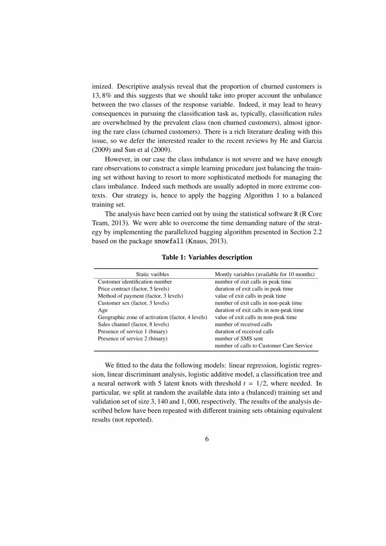
This section illustrates how the bagging applies to a real dataset of an Eu-ropean telecommunications company available at azzalini.stat.unipd.it/Book-DM/data.html. The dataset consists of 30,619 customers for which arecollected 99 variables. Among them some are static socio-demographic variablesrelated to the customer or to his/her contractual plan and other are dynamic vari-ables available each month, e.g. duration and number of phone calls, text mes-sages, and so forth, for the 10 months before the target event (churn or not). Adetailed list of the variables is shown in Table 1.

The datased is construct to mimic the operative behavior of a company. Atmonth t data for the 10 previous months will be available and the prediction forchurn at month t + 1 would be performed. Note that, as commonly done in thesedata mining context, the monthly variables are trated as independent, and withoutconsidering their natural dynamic dependence.

The application context requires that the number of churned customer notpredicted as such needs to be low, i.e. the false negative error rate must be min-

5

imized. Descriptive analysis reveal that the proportion of churned customers is13, 8% and this suggests that we should take into proper account the unbalancebetween the two classes of the response variable. Indeed, it may lead to heavyconsequences in pursuing the classification task as, typically, classification rulesare overwhelmed by the prevalent class (non churned customers), almost ignor-ing the rare class (churned customers). There is a rich literature dealing with thisissue, so we defer the interested reader to the recent reviews by He and Garcia(2009) and Sun et al (2009).

However, in our case the class imbalance is not severe and we have enoughrare observations to construct a simple learning procedure just balancing the train-ing set without having to resort to more sophisticated methods for managing theclass imbalance. Indeed such methods are usually adopted in more extreme con-texts. Our strategy is, hence to apply the bagging Algorithm 1 to a balancedtraining set.

The analysis have been carried out by using the statistical software R (R CoreTeam, 2013). We were able to overcome the time demanding nature of the strat-egy by implementing the parallelized bagging algorithm presented in Section 2.2based on the package snowfall (Knaus, 2013).

Table 1: Variables description

Static varibles Montly variables (available for 10 months)Customer identification number number of exit calls in peak timePrice contract (factor, 5 levels) duration of exit calls in peak timeMethod of payment (factor, 3 levels) value of exit calls in peak timeCustomer sex (factor, 3 levels) number of exit calls in non-peak timeAge duration of exit calls in non-peak timeGeographic zone of activation (factor, 4 levels) value of exit calls in non-peak timeSales channel (factor, 8 levels) number of received callsPresence of service 1 (binary) duration of received callsPresence of service 2 (binary) number of SMS sent

number of calls to Customer Care Service

We fitted to the data the following models: linear regression, logistic regres-sion, linear discriminant analysis, logistic additive model, a classification tree anda neural network with 5 latent knots with threshold t = 1/2, where needed. Inparticular, we split at random the available data into a (balanced) training set andvalidation set of size 3, 140 and 1, 000, respectively. The results of the analysis de-scribed below have been repeated with different training sets obtaining equivalentresults (not reported).

6

Figure 1 shows the global error evaluated under each model in function ofthe number of bootstrap iterations. The global errors reported are evaluated withrespect to the validation sample. These plots confirm what is stated in Breiman(1996). In our application the worst classifiers are heavily improved. For instance,the bagged version of the linear model reaches a global error of 18%, startingfrom an error of 31.5%. Clearly, the classifiers that already performed well areimproved but not considerably, e.g. using the GAM model the global error startsat 19.4% and ends with “only” 14.4%.

The plots in Figure 2 show the smoothed version of the global error, thefalse positive and false negative rates. These plots are very interesting since theysummarize all the information about the behavior of the bagging classifier. Inparticular it can be seen that only few classifiers are of particular interest in churnprediction since the goal is the minimization of the false negative rate. Theseclassifiers are the linear model and the neural net, as we can see from plot (a) and(e) of Figure 2; the remaining models produce bagging classifiers that have a falsenegative rate always bigger than the global error rate.

4. Conclusion

The results of all the methods are reported in Table 2. The global error is de-creased using bagging procedures. The improvement on the overall error has notthe same magnitude across the two components of the errors: false positives andfalse negatives. In fact, the false negatives are not really decreased while the falsepositives strongly turn down. Only the bagged neural network has an appreciabledecrease of both the components of the classification error and in particular of thefalse negative rate. This is probably due to the fact that the validation sample isunbalance and so the main improvement interests especially the majority of theobservations, i.e. those with y = 0.

From a marketing viewpoint, the improvement in the classification of the cus-tomer, according to their churn-propensity, allows several strategies. For example,it allows to better allocate marketing budget to the most likely leaving customer(possibly weighted for their monetary value) or to route incoming calls to the cus-tomer care more efficiently according to the estimated propensity of leaving. Thepredictive gain of the methods discussed here, has a direct effect on the efficiencyof any possible marketing operations.

From an operative viewpoint, the parallel implementation of such a meth-ods is appealing for practitioners that are stressed to produce reliable results inreasonable time.

7

0 100 200 300 400 500

0.10

0.15

0.20

0.25

0.30

Bagged linear model

iteration

Glo

bal e

rror

(a)

0 100 200 300 400 500

0.10

0.15

0.20

0.25

0.30

Bagged logistic model

iteration

Glo

bal e

rror

(b)

0 100 200 300 400 500

0.15

0.20

0.25

0.30

0.35

0.40

Bagged LDA

iteration

Glo

bal e

rror

(c)

0 100 200 300 400 500

0.17

00.

172

0.17

40.

176

Bagged classification tree

iteration

Glo

bal e

rror

(d)

0 100 200 300 400 500

0.14

0.16

0.18

0.20

0.22

0.24

Bagged neural net

iteration

Glo

bal e

rror

(e)

0 100 200 300 400 500

0.14

0.15

0.16

0.17

0.18

0.19

Bagged logistic GAM

iteration

Glo

bal e

rror

(f)

Figure 1: Global error on the validation sample

8

0 100 200 300 400 500

0.0

0.1

0.2

0.3

0.4

0.5

iteraion

Global errorFalse positiveFalse negative

(a)

0 100 200 300 400 500

0.0

0.1

0.2

0.3

0.4

0.5

iteraion

Global errorFalse positiveFalse negative

(b)

0 100 200 300 400 500

0.0

0.1

0.2

0.3

0.4

0.5

iteraion

Global errorFalse positiveFalse negative

(c)

0 100 200 300 400 500

0.0

0.1

0.2

0.3

0.4

0.5

iteraion

Global errorFalse positiveFalse negative

(d)

0 100 200 300 400 500

0.0

0.1

0.2

0.3

0.4

0.5

iteraion

Global errorFalse positiveFalse negative

(e)

0 100 200 300 400 500

0.0

0.1

0.2

0.3

0.4

0.5

iteraion

Global errorFalse positiveFalse negative

(f)

Figure 2: Smoothed global error and its components

9

Table 2: Global error, false positive error and false negative error rates forthe real data application

Basic methods BaggingGlobal False False Global False Falseerror negative positive error negative positive

linear model 33.97 9.02 77.59 16.21 10.84 17.13logistic regression 34.46 9.08 77.87 8.72 16.93 7.14discriminant analysis 33.97 9.02 77.59 15.91 26.61 14.19classification tree 24.94 9.55 72.64 17.44 19.32 11.47neural net 40.32 10.90 81.88 19.35 4.33 21.76logistic GAM 31.75 8.49 75.86 14.86 19.14 14.10

To conclude, if companies introduce bagging versions of their commonlyused classificators, they might better identify the riskiest customer and thus im-prove their retention rates.

Acknowledgements

The authors thank Bruno Scarpa for his suggestions in early versions of thepaper and the Associate Editor and the referees for comments. This work has beencarried out during the PhD studies of the authors at the Department of Statistics,University of Padua, Italy.

References

Bolton R, Kannan P, Bramlett M (2000) Implications of loyalty program mem-bership and service experiences for customer retention and value. Journal ofthe Academy of Marketing Science 28:95–108

Breiman L (1996) Bagging predictors. Machine Learning 24:123–140

Breiman L, Friedman J, Olshen R, Stone C (1984) Classification and RegressionTrees. Wadsworth and Brooks, Monterey, CA

Ganesh J, Arnold M, Reynold K (2000) Understanding the customer base of ser-vice providers: An examination of the differences between switchers and stay-ers. Journal of Marketing 64:65–87

Grama A (2003) Introduction to parallel computing. Pearson Education

10

Hastie T, Tibshirani R (1999) Generalized Additive Models. Chapman & Hall Ltd

Hastie T, Tibshirani R, Friedman J (2009) Elements of Statistical Learning.Springer

He H, Garcia EA (2009) Learning from imbalanced data. IEEE Transaction onKnowledge and Data Engineering 21(9)

Knaus J (2013) R package snowfall: Easier cluster computing (based on snow).URL http://CRAN.R-project.org/package=snowfall

Mardia K, Kent J, Bibby J (1979) Multivariate analysis. Academic Press

Neslin S, Gupta S, Kamakura W, Lu J, Mason C (2006) Defection detection: Mea-suring and understanding the predictive accuracy of customer churn models.Journal of Marketing Research 43:204–211

R Core Team (2013) R: A Language and Environment for Statistical Computing.R Foundation for Statistical Computing, URL http://www.R-project.org/

Shaffer G, Zhang J (2002) Competitive one-to-one promotions. Management Sci-ence 48:1143–1160

Strouse K (2004) Customer-centered telecommunications services marketing.Artech House Inc.

Sun Y, Wong AKC, Kamel MS (2009) Classification of imbalanced data: a re-view. International Journal of Pattern Recognition and Artificial Intelligence23(4):687–719

11