assessment and scenarios aassessment and scenar … · aaassessment and scenarios ssessment and...

AAAASSESSMENT AND SCENARSSESSMENT AND SCENARSSESSMENT AND SCENARSSESSMENT AND SCENARIOS IOS IOS IOS

OF LAND USE CHANGE IOF LAND USE CHANGE IOF LAND USE CHANGE IOF LAND USE CHANGE IN N N N

EEEEUROPEUROPEUROPEUROPE

Content: RIKS BV

Layout: RIKS BV

Illustrations: RIKS BV

Published by: RIKS BV

© RIKS BV (November 2008)

This is a publication of the Research Institute for Knowledge Systems (RIKS BV), Witmakersstraat 10, P.O. Box 463, 6200 AL Maastricht, The Netherlands, http://www.riks.nl, e-mail: [email protected], Tel. +31(0)433501750, Fax. +31(0)3501751.

Product information

Service Contract Nº 070307/2007/484442/MAR/B2: Natura 2000 preparatory actions, Lot 3: Developing New concepts for integration of the Natura 2000 network into a broader countryside

Assessment and scenarios of land Assessment and scenarios of land Assessment and scenarios of land Assessment and scenarios of land

use change in Europeuse change in Europeuse change in Europeuse change in Europe

© RIKS BV (November 2008)

Coordinator of RIKS work in this project:

• Hedwig van Delden

Contributing researchers (in alphabetical order):

• Alex Hagen

• Patrick Luja

• Yu-e Shi

• Jasper van Vliet

Research Institute for Knowledge Systems BV P. O. Box 463 6200 AL Maastricht The Netherlands www.riks.nl

I

ContentsContentsContentsContents

INTRODUCTION.................................................................................................................III

1. ANALYSIS OF HISTORIC LAND USE CHANGES...................................................... 5

1.1 Methodology ................................................................................................................ 5

1.2 Data .............................................................................................................................. 7

1.3 Land use change analysis ............................................................................................. 9

1.4 Conclusion of land use change analysis ..................................................................... 38

2. THE METRONAMICA MODEL.................................................................................... 41

3. CALIBRATION OF THE LAND USE MODEL ........................................................... 45

3.2 Assessment methods for the calibration results.......................................................... 46

3.3 Calibration results....................................................................................................... 48

3.4 Conclusion of the calibration results .......................................................................... 53

4. SCENARIOS...................................................................................................................... 55

4.1 Applications for scenarios .......................................................................................... 55

4.2 Procedure to create scenario input.............................................................................. 56

4.3 Analysis of results ...................................................................................................... 60

4.4 Conclusion of the scenario study................................................................................ 69

REFERENCES ...................................................................................................................... 71

APPENDIX A: NUTS-2 REGIONS..................................................................................... 73

III

IntroductionIntroductionIntroductionIntroduction

This report is prepared in the context the project Natura 2000 Preparatory Actions, Lot 3: Developing new concepts for integration of the Natura 2000 network into a broader countryside (Reference: ENV.B.2/SER/2007/0076). The aim of this project is to elaborate a new spatial vision for a green structure of the European Union and to ensure sustainable management of natural resources, adaptation to accelerated climate change and maintenance of biodiversity.

In this project, RIKS’ tasks are threefold:

1. To assess the historic land use changes in Europe based on Corine land cover data at 1 km resolution,

2. To use the information obtained under (1) to improve the calibration of the METRONAMICA land use model and to allow for a region-specific calibration rather than one set of parameter settings for EU-27,

3. To run the METRONAMICA land use model from 2000 until 2015 for the baseline scenarios from ESPON and from 2000 until 2030 for two different socio-economic scenarios provided by TERSYN.

The underlying document describes the data, methodologies and results of the historic analysis in chapter one. Next, an overview of the METRONAMICA model is provided and details the drivers of land use changes incorporated in this model and the parameters that have to be tuned. Chapter three follows with the procedure and results of the calibration carried out as part of this project. In chapter four we describe the procedure for converting the socio-economic scenarios into model input and discuss the results of the scenario runs.

5

1.1.1.1. Analysis of historic land use Analysis of historic land use Analysis of historic land use Analysis of historic land use

changeschangeschangeschanges

1.11.11.11.1 MethodologyMethodologyMethodologyMethodology

For the analysis of historic land use changes we look at developments that have occurred between 1990 and 2000 in the Corine land cover (CLC) maps. Because the CLC2006 map was not available at the time of the analysis, this map is not included in the analysis.

The results of the historic analysis will be used in the next step to provide information for parameter settings of the calibration as well as the future developments in the baseline scenario. For this reason the analysis focuses on those land use classes that will be modelled explicitly in the land use model. The selected land use model is METRONAMICA, which is incorporated among others in the LUMOCAP Policy Support System (PSS). This land use model is applied to EU-27 at a 1 km resolution, consistent with the resolution of this analysis. As part of the LUMOCAP project1, it is already calibrated with a single parameter set that applies to EU-27 as a whole. From this experience we learned that there are regional differences that cannot be discarded. Therefore in the current project we have divided Europe in a few major regions (described further below) for which different parameter settings will be applied.

To be able to build on the existing calibration from the LUMOCAP project, the land use categories that will be analysed for the period 1990-2000 and that will be modelled dynamically in the land use model are:

• Residential areas,

• Industry & commerce,

• Tourism & recreation,

• Agriculture,

• Forest, and

• Natural vegetation.

Understanding land use change is more than merely looking at the total area of certain land uses that appeared or disappeared. Also the change in structure and the underlying reasons of this change are important. It is the complete picture of different elements that provides insight in land use changes. For this reason we have focused on three particular ways to measure the change:

1. Appearance and disappearance:

In this part of the analysis we provide an overview of observed changes in area in the 6 classes mentioned above. Results from this analysis are:

a) Total area per land use in 1990,

1 www.riks.nl/projects/lumocap

6

b) Total area per land use in 2000,

c) Absolute change in area per land use from 1990 to 2000,

d) Surface share per land use in 1990,

e) Surface share per land use in 2000,

f) Increase or decrease from 1990 to 2000 per land use function, expressed relative to the original (1990) amount of land use for that function,

g) Increase or decrease from 1990 to 2000 per land use function, expressed as a percentage of the total land area.

2. Growth and shrink of different land use categories:

In this part of the analysis we provide an overview of observed changes in area in the 6 classes mentioned above. Results from this analysis are:

a) For locations in which in 2000 new land use functions appear we analyse what land use this location had in 1990 and what the neighbouring land use of this location was in 1990, both representing pull factors.

b) For locations in which in 2000 land use functions have disappeared we analyse what land use this location had in 1990 and what the neighbouring land use in this location was in 1990, representing push factors.

3. Cluster size change of different land use categories:

We use two different measures for analysing the cluster size change:

a) For the residential clusters we calculate the cluster size – frequency distribution which shows the distribution of the different residential cluster sizes in a certain area.

b) For all six classes we calculate the clumpiness index2 as landscape metric, which can be used to characterize the landscape pattern in an area.

The analysis has been carried out at two different spatial scales, at NUTS-2 level and at the level of groups of countries that we expect would have similar behaviour. Based on geographical location and history we have selected the following groups of countries3: Western Europe (Austria, Belgium, Denmark France, Germany, Ireland, Luxembourg, the Netherlands); North-eastern Europe (Czech Republic, Poland, Slovakia,); South-eastern Europe (Bulgaria, Hungary, Romania, Slovenia); Mediterranean (Italy, Greece, Portugal, Spain); and the Baltic states (Estonia, Latvia, Lithuania).

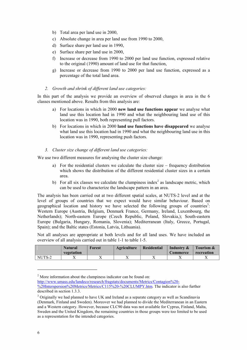
Not all analyses are appropriate at both levels and for all land uses. We have included an overview of all analysis carried out in table 1-1 to table 1-5.

Natural

vegetation

Forest Agriculture Residential Industry &

Commerce

Tourism &

recreation

NUTS-2 X X X X X X

2 More information about the clumpiness indicator can be found on: http://www.umass.edu/landeco/research/fragstats/documents/Metrics/Contagion%20-%20Interspersion%20Metrics/Metrics/C115%20-%20CLUMPY.htm. The indicator is also further described in section 1.3.3. 3 Originally we had planned to have UK and Ireland as a separate category as well as Scandinavia (Denmark, Finland and Sweden). Moreover we had planned to divide the Mediterranean in an Eastern and a Western category. However, because CLC90 data was not available for Cyprus, Finland, Malta, Sweden and the United Kingdom, the remaining countries in those groups were too limited to be used as a representation for the intended categories.

7

Natural

vegetation


Commerce

Tourism &

recreation

Country groups

X X X X X X

Table 1-1 Overview of analysis of appearance and disappearance of land use functions

Natural

vegetation


Commerce

Tourism &

recreation

NUTS-2 X X X Country groups

X X X X X X

Table 1-2 Overview of analysis of the neighbourhood characteristics of locations for land new

land use functions

Natural

vegetation


Commerce

Tourism &

recreation

NUTS-2 X X Country groups

X X X X X X

Table 1-3 Overview of analysis of the neighbourhood of land uses that have disappeared

Natural

vegetation


Commerce

Tourism &

recreation

NUTS-2 Country groups

X

Table 1-4 Overview of analysis of the cluster size – frequency distribution

Natural

vegetation


Commerce

Tourism &

recreation

NUTS-2 X X X X X X Country groups

X X X X X X

Table 1-5 Overview of analysis of the Clumpiness Index

1.21.21.21.2 DataDataDataData

1.2.1 Land use maps

For the analysis of historic developments, Corine land cover (CLC) maps for 1990 and 2000 are used to assess the trends of land use and cover change over this period. For this analysis the original CLC maps were aggregated to a spatial resolution of 1 km2 using an adjusted majority aggregation. For this method an additional constraint was added to the aggregation procedure to make sure that the total area per land use function remains the same before and after the aggregation.

CLC 1990 is not available for Cyprus, Finland, Malta, Sweden and United Kingdom. Hence for the land use change analysis for 1990 to 2000, no results can be obtained for these countries.

1.2.2 Land use classification

For this analysis we reclassified the CLC land use classes to more aggregated ones. Those are the classes that are currently modelled in a dynamic manner in the METRONAMICA land

8

use model included in the LUMOCAP PSS. The reclassification of CLC classes is shown in table 1-6. This table also shows a categorisation of land use classes into functions, features and vacant states, which is required for METRONAMICA

4. In the METRONAMICA application for the current project, natural vegetation is considered as vacant state; agriculture, industry & commerce, residential areas, tourism & recreation and forest are functions; the rest of the land cover classes are considered features.

LUMOCAP classes Type CLC code CLC classes

Natural vegetation Vacant 321 Natural grasslands Natural vegetation Vacant 322 Moors and heathland Natural vegetation Vacant 323 Sclerophyllous vegetation Natural vegetation Vacant 324 Transitional woodland-shrub Agriculture Function 211 Non-irrigated arable land Agriculture Function 212 Permanently irrigated land Agriculture Function 213 Rice fields Agriculture Function 221 Vineyards Agriculture Function 222 Fruit trees and berry plantations Agriculture Function 223 Olive groves Agriculture Function 231 Pastures Agriculture Function 241 Annual crops associated with permanent

crops Agriculture Function 242 Complex cultivation patterns Agriculture Function 244 Agro-forestry areas Agriculture Function 243 Land principally occupied by agriculture,

with significant areas of natural vegetation

Residential areas Function 111 Continuous urban fabric Residential areas Function 112 Discontinuous urban fabric Industry and Commerce Function 121 Industrial or commercial units Tourism and Recreation Function 141 Green urban areas Tourism and Recreation Function 142 Sport and leisure facilities Forest Function 311 Broad-leaved forest Forest Function 312 Coniferous forest Forest Function 313 Mixed forest Open spaces with little or no vegetation

Feature 332 Bare rocks

Open spaces with little or no vegetation

Feature 333 Sparsely vegetated areas


Feature 334 Burnt areas


Feature 335 Glaciers and perpetual snow

Infrastructure Feature 122 Road and rail networks and associated land

4Features are land use classes that are not supposed to change in the simulation, like water bodies or airports. Functions are land use classes that are actively modelled, like residential or industry & commerce. Functions change dynamically as the result of the local and the regional dynamics. Vacant states finally are classes that are only changing as a result of other land use dynamics. Computationally at least one vacant state is required. Typically abandoned land or natural land use types are modelled as vacant state, since they are literally vacant for other land uses or the result of the disappearance of other land use functions.

9

LUMOCAP classes Type CLC code CLC classes

Port Area Feature 123 Port areas Airports Feature 124 Airports Mineral extraction sites Feature 131 Mineral extraction sites Dump sites Feature 132 Dump sites Inland wetlands Feature 411 Inland marshes Inland wetlands Feature 412 Peat bogs Marine wetlands Feature 421 Salt marshes Marine wetlands Feature 422 Salines Marine wetlands Feature 423 Intertidal flats Inland water bodies Feature 511 Water courses Inland water bodies Feature 512 Water bodies Marine water bodies Feature 521 Coastal lagoons Marine water bodies Feature 522 Estuaries Marine water bodies Feature 523 Sea and ocean Beaches, dunes, sands Feature 331 Beaches, dunes, sands * 133 Construction sites Land outside modelling area Feature 990 UNCLASSIFIED LAND SURFACE Water outside modelling area

Feature 995 UNCLASSIFIED WATER BODIES

Table 1-6 Corine land cover classes (level 3) and LUMOCAP land cover classes.

*Construction (133) is converted to the land use class of the surrounding build-up area.

1.31.31.31.3 Land use change analysisLand use change analysisLand use change analysisLand use change analysis

This section provides the results of the different parts of the historical analysis described in the methodology section (1.1):

• Appearance and disappearance of different land use categories

• Growth and shrink of different land use categories

• Cluster size change of different land use categories

Most of the analysis is carried out at NUTS-2 level (see appendix I for an overview of all 261 NUTS-2 regions in EU-27) and at the level of the country groups (see table 1-7). We found that most NUTS-2 regions contain only a small number of cells per land use class that actually change. Results of an analysis based on only a few cells are not significant and therefore not meaningful for the current purpose. For this reason we describe below the results for the groups of countries.

NUTS-0 Name Group of countries

EE Estonia Baltic states LT Lithuania Baltic states LV Latvia Baltic states CZ Czech Republic North-eastern Europe PL Poland North-eastern Europe SK Slovakia North-eastern Europe BG Bulgaria South-eastern Europe HU Hungary South-eastern Europe RO Romania South-eastern Europe SI Slovenia South-eastern Europe ES Spain Mediterranean

10

NUTS-0 Name Group of countries

GR Greece Mediterranean IT Italy Mediterranean PT Portugal Mediterranean AT Austria Western Europe BE Belgium Western Europe DE Germany Western Europe DK Denmark Western Europe FR France Western Europe IE Ireland Western Europe LU Luxemburg Western Europe NL The Netherlands Western Europe CY Cyprus Excluded FI Finland Excluded MT Malta Excluded SE Sweden Excluded UK United Kingdom Excluded

Table 1-7 Group of countries list

1.3.1 Appearance and disappearance of land use

The result of appearance and disappearance analysis shows the overview of observed changes in the 6 classes mentioned above. Results for group of countries include:

• Total area per land use per group of countries in 1990 (see table 1-8),

• Total area per land use per group of countries in 2000 (see table 1-8),

• Absolute change of area per land use per group of countries from 1990 to 2000 (see table 1-8 and ¡Error! No se encuentra el origen de la referencia., 1-3, 1-5, 1-7, 1-9 and 1-11),

• Surface share per land use class per group of countries in 1990, which is calculated by its total area in 1990 divided by the total area of the group of countries (see table 1-9),

• Surface share per land use class per group of countries in 2000, which is calculated by its total area in 2000 divided by the total area of the group of countries (see table 1-10),

• Increase or decrease from 1990 to 2000 per land use function, expressed relative to the original (1990) amount of land use for that function (see table 1-121 and figures 1-2, 1-4, 1-6, 1-8, 1-10 and 1-12),

• Increase or decrease from 1990 to 2000 per land use function, expressed as a percentage of the total land area (see table 1-12).

Region Presence in

maps

Natural

vegetation

Agriculture Residential

areas

Industry

&

Commerce

Tourism

&

Recreation

Forest Total

Baltic States 1990 9356 82977 2516 718 227 69615 165409 Baltic States 2000 12146 83219 2531 726 226 66534 165382 Baltic States Present in

both maps 9272 82769 2511 714 224 66457 161947

Baltic States Only in 1990

84 208 5 4 3 3158 3462

11

Region Presence in

maps

Natural

vegetation


areas

Industry

&

Commerce

Tourism

&

Recreation

Forest Total

Baltic States Only in 2000

2874 450 20 12 2 77 3435

Baltic States Difference 2000-1990

2790 242 15 8 -1 -3081 6137

Baltic States Total change 2000-1990

2958 658 25 16 5 3235 6897

North-eastern 1990 7072 271833 13534 1760 897 136144 431240 North-eastern 2000 7403 271062 13747 1832 904 136302 431250 North-eastern Present in

both maps 4949 270609 13497 1748 875 133815 525493

North-eastern Only in 1990

2123 1224 37 12 22 2329 5747

North-eastern Only in 2000

2454 453 250 84 29 2487 5757

North-eastern Difference 2000-1990

331 -771 213 72 7 158 1552

North-eastern Total change 2000-1990

4577 1677 287 96 51 4816 11504

South-eastern 1990 27623 262485 21511 2645 620 132320 447204 South-eastern 2000 27143 261843 21588 2701 629 133194 447098 South-eastern Present in

both maps 25340 261295 21468 2635 615 130680 442033

South-eastern Only in 1990

2283 1190 43 10 5 1640 5171

South-eastern Only in 2000

1803 548 120 66 14 2514 5065

South-eastern Difference 2000-1990

-480 -642 77 56 9 874 2138

South-eastern Total change 2000-1990

4086 1738 163 76 19 4154 10236

Mediterranean 1990 232595 507804 17808 3064 556 218916 980743 Mediterranean 2000 230623 505517 19995 4043 765 218888 979831 Mediterranean Present in

both maps 220111 500858 17680 3004 530 209995 952178

Mediterranean Only in 1990

12484 6946 128 60 26 8921 28565

Mediterranean Only in 2000

10512 4659 2315 1039 235 8893 27653

Mediterranean Difference 2000-1990

-1972 -2287 2187 979 209 -28 7662

Mediterranean Total change 2000-1990

22996 11605 2443 1099 261 17814 56218

Western Europe

1990 51651 701699 54390 6305 3695 303651 1121391

Western Europe

2000 53304 695822 57285 7860 4371 303464 1122106

Western Europe

In both 47006 694402 54084 6231 3621 297816 1103160

Western Europe

Only in 1990

4645 7297 306 74 74 5835 18231

12

Region Presence in

maps

Natural

vegetation


areas

Industry

&

Commerce

Tourism

&

Recreation

Forest Total

Western Europe

Only in 2000

6298 1420 3201 1629 750 5648 18946

Western Europe

Difference 2000-1990

1653 -5877 2895 1555 676 -187 12843

Western Europe

Difference 2000-1990

10943 8717 3507 1703 824 11483 37177

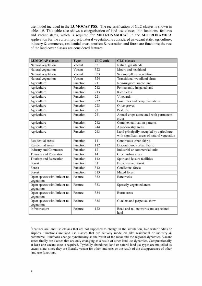
Table 1-8 Absolute change of area in km² per group of countries between 1990 and 2000

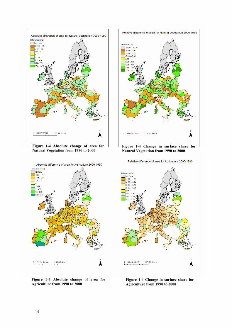
Table 1-8 shows that there was an increase in residential and industrial & commercial locations in the period 1990-2000 in all 5 groups of countries. On the other hand, there was a large decrease in agricultural areas in the same period. The only exceptions are the Baltic States, where we observe a large increase. This increase comes at the cost of forested areas, which indicates that forests are being cleared for agriculture. In this region we also see an emergence of natural vegetation over the period 1990-2000 which could be the result of forest harvesting.

Some new forest appears in 2000 in North-eastern Europe and South-eastern Europe, while there is a small decline in the Mediterranean and Western Europe. But more than that, we see a large relocation of forests in these countries. For example, the Mediterranean had a net loss of only 28 km² of forest between 1990 and 2000. But in the same period, there was 8865 km² of forest reallocated. Since changes of a similar extend are visible for natural vegetation, it could very well be that these changes are due to classification errors, since there is a thin line between forest and natural vegetation. Finally, we see an increase of tourism & recreation over the period 1990-2000 in most countries, with Western Europe and the Mediterranean the countries where we observe the largest growth.

Natural

vegetation

Agriculture Residential Industry

&

Commerce

Tourism &

Recreation

Forest

Baltic states 5.37% 47.60% 1.44% 0.41% 0.13% 39.93% North-eastern Europe 1.61% 61.72% 3.07% 0.40% 0.20% 30.91% South-eastern Europe 5.97% 56.73% 4.65% 0.57% 0.13% 28.60% Mediterranean 22.63% 49.41% 1.73% 0.30% 0.05% 21.30% Western Europe 4.38% 59.56% 4.62% 0.54% 0.31% 25.77%

Table 1-9 Surface share per land use per group of countries in 1990

Natural

vegetation


&

Commerce

Tourism &

Recreation

Forest

Baltic states 6.97% 47.73% 1.45% 0.42% 0.13% 38.16% North-eastern Europe 1.68% 61.55% 3.12% 0.42% 0.21% 30.95% South-eastern Europe 5.87% 56.59% 4.67% 0.58% 0.14% 28.78% Mediterranean 22.44% 49.19% 1.95% 0.39% 0.07% 21.30% Western Europe 4.52% 59.06% 4.86% 0.67% 0.37% 25.76%

Table 1-10 Surface share per land use per group of countries in 2000

13

Natural

vegetation


&

Commerce

Tourism &

Recreation

Forest

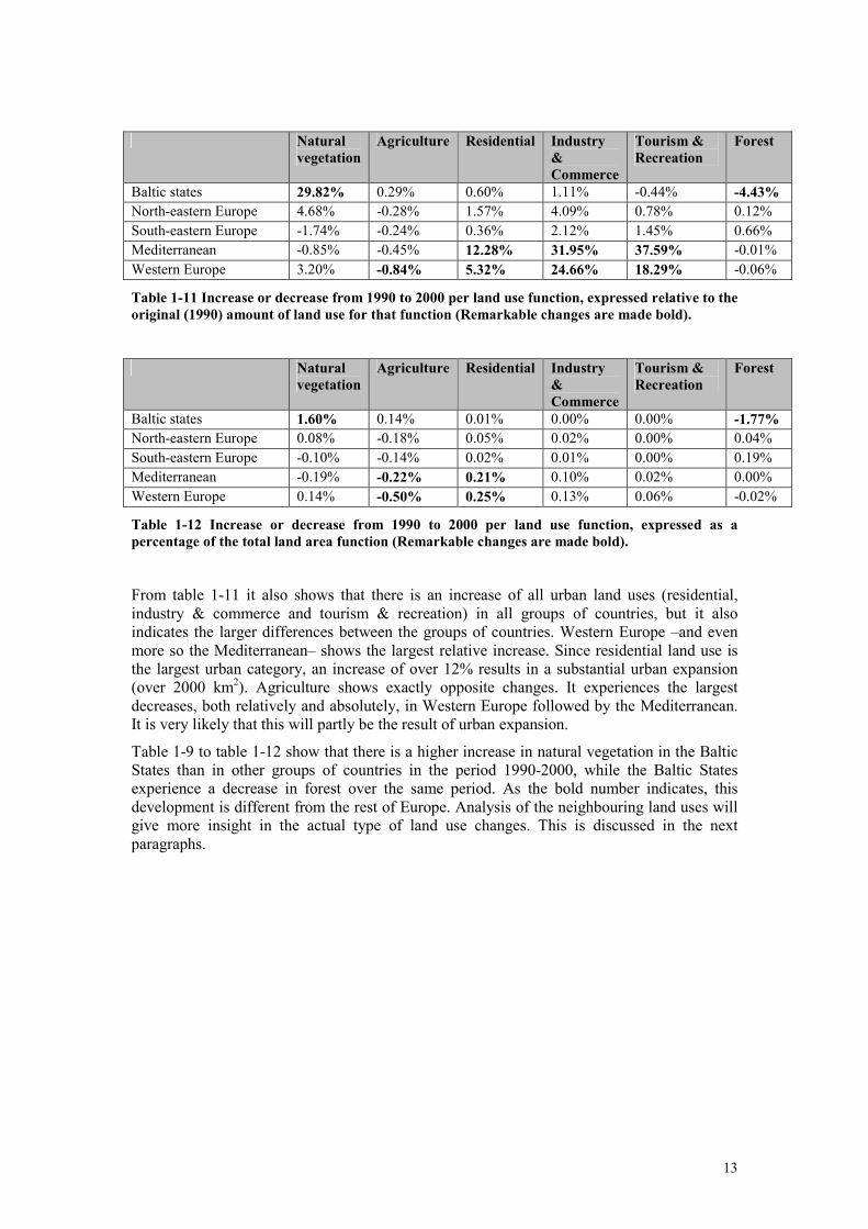
Baltic states 29.82% 0.29% 0.60% 1.11% -0.44% -4.43%

North-eastern Europe 4.68% -0.28% 1.57% 4.09% 0.78% 0.12% South-eastern Europe -1.74% -0.24% 0.36% 2.12% 1.45% 0.66% Mediterranean -0.85% -0.45% 12.28% 31.95% 37.59% -0.01% Western Europe 3.20% -0.84% 5.32% 24.66% 18.29% -0.06%

Table 1-11 Increase or decrease from 1990 to 2000 per land use function, expressed relative to the

original (1990) amount of land use for that function (Remarkable changes are made bold).

Natural

vegetation


&

Commerce

Tourism &

Recreation

Forest

Baltic states 1.60% 0.14% 0.01% 0.00% 0.00% -1.77%

North-eastern Europe 0.08% -0.18% 0.05% 0.02% 0.00% 0.04% South-eastern Europe -0.10% -0.14% 0.02% 0.01% 0.00% 0.19% Mediterranean -0.19% -0.22% 0.21% 0.10% 0.02% 0.00% Western Europe 0.14% -0.50% 0.25% 0.13% 0.06% -0.02%

Table 1-12 Increase or decrease from 1990 to 2000 per land use function, expressed as a

percentage of the total land area function (Remarkable changes are made bold).

From table 1-11 it also shows that there is an increase of all urban land uses (residential, industry & commerce and tourism & recreation) in all groups of countries, but it also indicates the larger differences between the groups of countries. Western Europe –and even more so the Mediterranean– shows the largest relative increase. Since residential land use is the largest urban category, an increase of over 12% results in a substantial urban expansion (over 2000 km2). Agriculture shows exactly opposite changes. It experiences the largest decreases, both relatively and absolutely, in Western Europe followed by the Mediterranean. It is very likely that this will partly be the result of urban expansion.

Table 1-9 to table 1-12 show that there is a higher increase in natural vegetation in the Baltic States than in other groups of countries in the period 1990-2000, while the Baltic States experience a decrease in forest over the same period. As the bold number indicates, this development is different from the rest of Europe. Analysis of the neighbouring land uses will give more insight in the actual type of land use changes. This is discussed in the next paragraphs.

14

Figure 1-4 Change in surface share for

Agriculture from 1990 to 2000


Natural Vegetation from 1990 to 2000

Figure 1-4 Absolute change of area for

Natural Vegetation from 1990 to 2000


Agriculture from 1990 to 2000

15


Forest from 1990 to 2000


Tourism and Recreation


Tourism and Recreation from 1990 to 2000


Forest from 1990 to 2000

16

R


Residential areas from 1990 to 2000

Figure 1-12 Change in surface share

for Industry and Commerce from

1990 to 2000


Residential areas from 1990 to 2000

Figure 1-12 Absolute change of area

for Industry and Commerce from

1990 to 2000

Residential 2000-1990

17

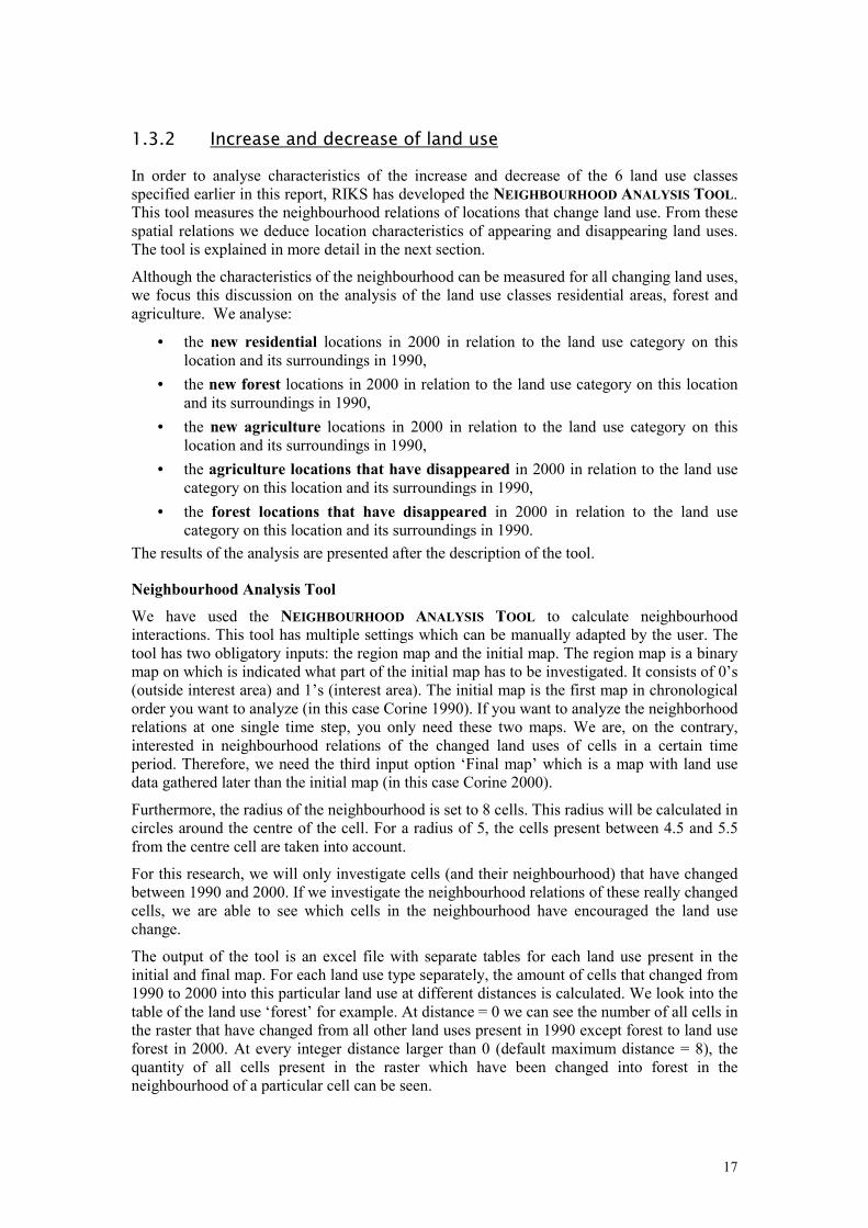
1.3.2 Increase and decrease of land use

In order to analyse characteristics of the increase and decrease of the 6 land use classes specified earlier in this report, RIKS has developed the NEIGHBOURHOOD ANALYSIS TOOL. This tool measures the neighbourhood relations of locations that change land use. From these spatial relations we deduce location characteristics of appearing and disappearing land uses. The tool is explained in more detail in the next section.

Although the characteristics of the neighbourhood can be measured for all changing land uses, we focus this discussion on the analysis of the land use classes residential areas, forest and agriculture. We analyse:

• the new residential locations in 2000 in relation to the land use category on this location and its surroundings in 1990,

• the new forest locations in 2000 in relation to the land use category on this location and its surroundings in 1990,

• the new agriculture locations in 2000 in relation to the land use category on this location and its surroundings in 1990,

• the agriculture locations that have disappeared in 2000 in relation to the land use category on this location and its surroundings in 1990,

• the forest locations that have disappeared in 2000 in relation to the land use category on this location and its surroundings in 1990.

The results of the analysis are presented after the description of the tool.

Neighbourhood Analysis Tool

We have used the NEIGHBOURHOOD ANALYSIS TOOL to calculate neighbourhood interactions. This tool has multiple settings which can be manually adapted by the user. The tool has two obligatory inputs: the region map and the initial map. The region map is a binary map on which is indicated what part of the initial map has to be investigated. It consists of 0’s (outside interest area) and 1’s (interest area). The initial map is the first map in chronological order you want to analyze (in this case Corine 1990). If you want to analyze the neighborhood relations at one single time step, you only need these two maps. We are, on the contrary, interested in neighbourhood relations of the changed land uses of cells in a certain time period. Therefore, we need the third input option ‘Final map’ which is a map with land use data gathered later than the initial map (in this case Corine 2000).

Furthermore, the radius of the neighbourhood is set to 8 cells. This radius will be calculated in circles around the centre of the cell. For a radius of 5, the cells present between 4.5 and 5.5 from the centre cell are taken into account.

For this research, we will only investigate cells (and their neighbourhood) that have changed between 1990 and 2000. If we investigate the neighbourhood relations of these really changed cells, we are able to see which cells in the neighbourhood have encouraged the land use change.

The output of the tool is an excel file with separate tables for each land use present in the initial and final map. For each land use type separately, the amount of cells that changed from 1990 to 2000 into this particular land use at different distances is calculated. We look into the table of the land use ‘forest’ for example. At distance = 0 we can see the number of all cells in the raster that have changed from all other land uses present in 1990 except forest to land use forest in 2000. At every integer distance larger than 0 (default maximum distance = 8), the quantity of all cells present in the raster which have been changed into forest in the neighbourhood of a particular cell can be seen.

18

The second step is to calculate the relative attraction of all land uses at a certain land use. We use a formula which resembles the enrichment factor of Verburg et al. (2004). The main difference is however, that we only look at cells of which the land use type has been changed between 1990 and 2000. The following formula will be used for this:

, ,, ,

,

/

/k l d k

k l d

k d

n nF

N N=

Fk,l,,d is the average relative attraction of land use k to land use l at a neighbourhood with distance d, nk,l,d is the number of cells of land use type l in the neighbourhood d which have been changed from 1990 to 2000 into land use type k, nk is the total number of cells which have been changed into land use type k between 1990 and 2000, Nk,d is the number of cells in the neighbourhood with distance d of all cells in the raster with land use type k and N are all cells in the raster.

The calculations will be done for all land uses present in the research area.

If for example, the neighbouring cells for land use forest at distance 3 consist of 50% agricultural land and the fraction of all cells in a country which have agriculture as neighbour at distance 3 equals 25%, the relative attraction of agriculture at forest at distance 3 is 2.

The final step is to transform all relative attraction values with a logarithmic function in order to get attraction and repulsion on the same scale. After this transformation, values larger than 0 indicate an attraction effect, values smaller than 0 indicate a repulsion effect and a value of 0 indicates that the land uses do not influence each other. Eventually, graphs can be created with attraction and repulsion values of every land use interaction.

Results of the neighbourhood analysis

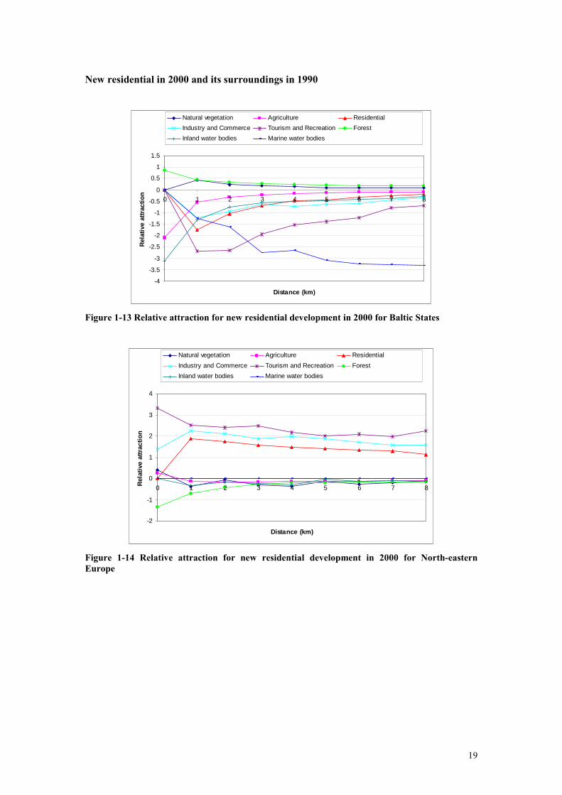
The results of this analysis are shown in the graphs below. Graphs represent the relation between the land use under investigation and its surroundings. On the x-axis you see the distance from the cell that changes land use, measured in km. On the y-axis you see the attracting (positive value) or repelling (negative value) effect of the different land uses. To obtain this relative attractiveness, neighbourhoods are compared with the average neighbourhood for the complete group of countries. As an example on figure 1-13 the positive values at distance 1-8 (1-8 km) for the red line (residential) indicate that new residential areas have a preference to locate near existing residential areas. The negative values for green (forest) at distance 1-8 indicate that new residential land uses are not so much attracted to forested areas.

The value at x = 0 represents the attraction of certain land uses to be taken over by the land use under investigation (e.g. in figure 1-13 we observe that more than on average new residential areas will appear on locations previously -in 1990- occupied by tourism & recreation and industry & commerce) or the attraction of a land use to occupy a location after the land use under investigation has disappeared (e.g. in figure 1-31 we see that locations in 1990 occupied by agriculture are more than average occupied by the urban land uses in 2000).

19

New residential in 2000 and its surroundings in 1990

-4

-3.5

-3

-2.5

-2

-1.5

-1

-0.5

0

0.5

1

1.5

0 1 2 3 4 5 6 7 8

Distance (km)

Rel

ativ

e at

trac

tio

n

Natural vegetation Agriculture Residential

Industry and Commerce Tourism and Recreation Forest

Inland water bodies Marine water bodies

Figure 1-13 Relative attraction for new residential development in 2000 for Baltic States

-2

-1

0

1

2

3

4

0 1 2 3 4 5 6 7 8

Distance (km)

Rel

ativ

e at

trac

tio

n




Figure 1-14 Relative attraction for new residential development in 2000 for North-eastern

Europe

20

-1.5

-1

-0.5

0

0.5

1

1.5

2

2.5

3

3.5

0 1 2 3 4 5 6 7 8

Distance (km)

Rre

lati

ve a

ttra

ctio

n




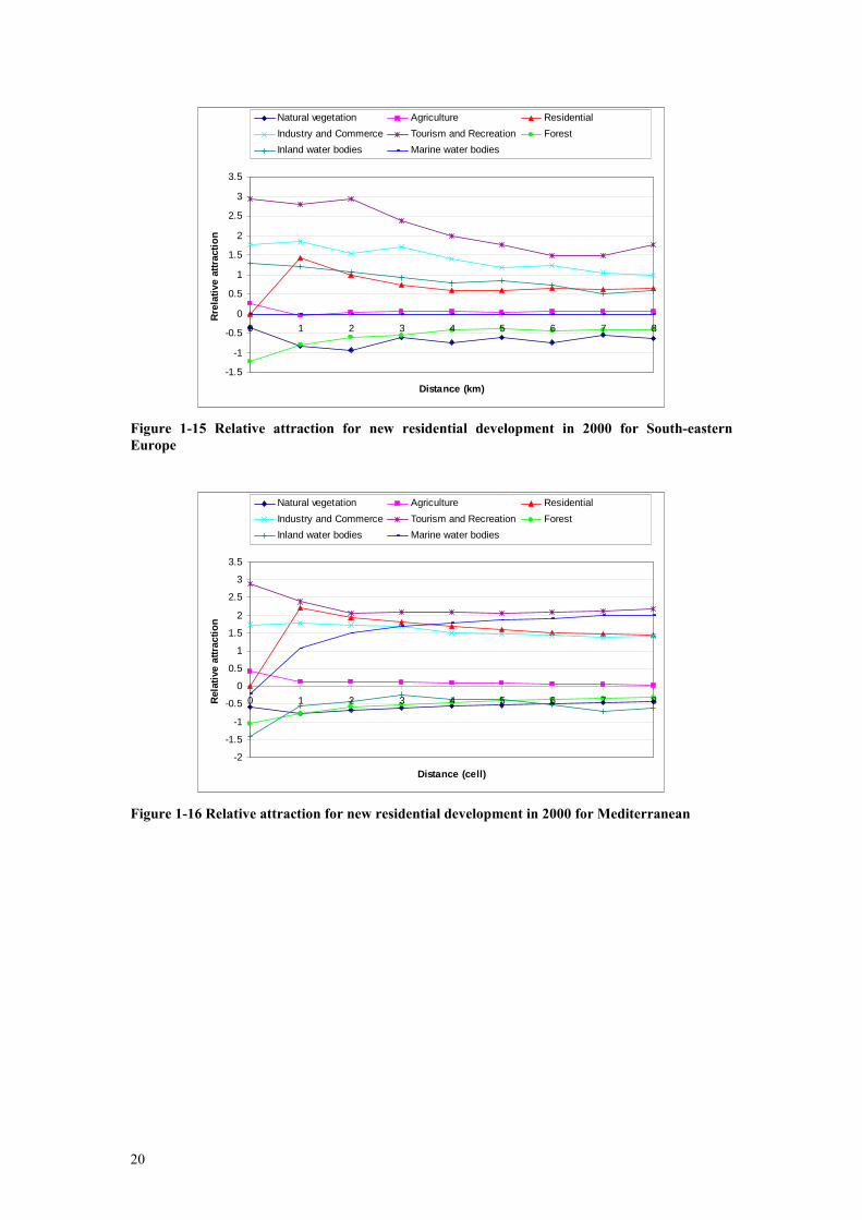
Figure 1-15 Relative attraction for new residential development in 2000 for South-eastern

Europe

-2

-1.5

-1

-0.5

0

0.5

1

1.5

2

2.5

3

3.5

0 1 2 3 4 5 6 7 8

Distance (cell)

Rel

ativ

e at

trac

tio

n




Figure 1-16 Relative attraction for new residential development in 2000 for Mediterranean

21

-2

-1.5

-1

-0.5

0

0.5

1

1.5

2

0 1 2 3 4 5 6 7 8

Distance (km)

Rel

ativ

e at

trac

tio

n




Figure 1-17 Relative attraction for new residential development in 2000 for Western Europe

Figure 1-13 to figure 1-17 show the relative attraction for new residential locations in 2000 per group of countries. In general, new residential land uses have replaced industry & commerce, tourism & recreation and agriculture in all groups of countries. The latter is the strongest in the Mediterranean and Western Europe and indicates urban expansion at the cost of agriculture. From the graph we see no attraction of new residential areas (2000) to allocate on areas occupied by natural vegetation or forest in 1990.

In most of the groups of countries there is a high number of new residential locations and from this we can conclude that the statements made above are reliable. In the Baltic States, there was only an increase of 20 new residential cells over the period 1990-2000. Thus, although the result of the analysis points in the same direction of that of the other groups of countries, the result for this region might not be significant.

The observed values for industry & commerce and tourism & recreation could be the result of classification differences, since both are urban fabric. Minor changes can cause the classification to change from the one in the other. Very often urban land uses are difficult to distinguish and it happens that in one year a location is classified as residential and in the next as tourism & recreation. To make hard statement on the allocation of residential areas in 2000 on locations previously occupied by industry & commerce and tourism & recreation we would have to carry out more research. From experience we know that in some countries (especially in Western Europe) industry is relocated away from city centres and the space that becomes available is taken in by other urban classes (very often residential). But, as said, this knowledge is not sufficient to make overall statements on the observed conversion.

We should also take into account in this analysis the fact that tourism & recreation covers a very small share of surface of the whole region (see table 1-9 and table 1-10). Therefore very few cells of that land use can cause a relatively strong effect in the overall figures.

The graphs indicate that tourism & recreation, industry & commerce and residential areas have a higher than average attraction on new residential land use to allocate in their surroundings. This effect becomes clear because of the positive value for the urban land uses at x=1 to x=8. Forest and natural vegetation seem to provide an attraction less than average and agriculture around the average. From this we can conclude that people prefer to build new residential locations close to existing urban land clusters. Forest and natural areas do not seem to have a special attraction and this can be because of a lack of infrastructure, accessibility and services, or because of zoning regulations that prohibit new residential development in certain locations and stimulate them in other locations.

22

The results include the attraction of inland water bodies and marine water bodies. These are not the main studied land use categories in the current project, but these figures do provide us with extra information about the relation between the urban land categories and water bodies. They show various attractions per group of countries. In South-eastern Europe and Western Europe, inland water bodies were attractive for new residential in 2000. In Mediterranean and Western Europe, marine water bodies were attractive for new residential in 2000. This effect is probably due to the historical preference of cities to locate next to the coast, the river or the lake and does not so much reflect current preferences.

The attraction of new residential developments to marine waters is in the Mediterranean already present at a direct distance (x = 1), while in Western Europe we observe this only at distances from the sea that are greater than 3 kilometres.

New Agriculture in 2000 and its surroundings in 1990

-3

-2.5

-2

-1.5

-1

-0.5

0

0.5

1

1.5

0 1 2 3 4 5 6 7 8

Distance (km)

Rel

ativ

e at

trac

tio

n




Figure 1-18 Relative attraction for new agricultural areas in 2000 for the Baltic States

-1

-0.5

0

0.5

1

1.5

2

2.5

3

0 1 2 3 4 5 6 7 8

Distance (kml)

Rel

ativ

e at

trac

tio

n




Figure 1-19 Relative attraction for new agricultural areas in 2000 for North-eastern Europe

23

-2.5

-2

-1.5

-1

-0.5

0

0.5

1

1.5

2

2.5

0 1 2 3 4 5 6 7 8

Distance (kml)

Rel

ativ

e at

trac

tio

n




Figure 1-20 Relative attraction for new agricultural areas in 2000 for South-eastern Europe

-2.5

-2

-1.5

-1

-0.5

0

0.5

1

1.5

0 1 2 3 4 5 6 7 8

Distance (km)

Rel

ativ

e at

trac

tio

n




Figure 1-21 Relative attraction for new agricultural areas in 2000 for Mediterranean

24

-1

-0.5

0

0.5

1

1.5

2

0 1 2 3 4 5 6 7 8

Distance (km)

Rel

ativ

e at

trac

tio

n




Figure 1-22 Relative attraction for new agricultural areas in 2000 for Western Europe

Figure 1-18 to figure 1-22 show the relative attraction for new agriculture in 2000 per group of countries. From these figures we can conclude that agriculture is often allocated on areas previously occupied by natural vegetation and to a lesser extent on areas previously occupied by forests. In the Baltic States we observe a different relation. Here, we see that agriculture has primarily replaced forested areas. This indicates the clearing of forests to provide space for agriculture. This conclusion underpins the conclusion made in the previous section where we noticed an increase in overall agricultural area and a decrease in overall forested area.

At larger distances (in the surrounding) agriculture seems to have a preference to allocate next to natural vegetation and –to a lesser extent– to forest, as opposed to urban land uses. The only exceptions are (1) the Mediterranean, where there is a clear preference to allocate near natural vegetation, while forest has an attraction less than average and (2) the Baltic States, where natural vegetation does not seem to be a land use that attracts agriculture, while forest has a strong attraction.

In North-eastern Europe we see an attraction of new agricultural areas to industry & commerce, while in the Baltic States and the Mediterranean we experience the opposite effect.

25

New forest in 2000 and its surroundings in 1990

-3

-2

-1

0

1

2

3

0 1 2 3 4 5 6 7 8

Distance (km)

Rel

ativ

e at

trac

tio

n




Figure 1-23 Relative attraction for new forest areas in 2000 for the Baltic States

-3

-2

-1

0

1

2

3

4

5

0 1 2 3 4 5 6 7 8

Distance (km)

Rel

ativ

e at

trac

tio

n




Figure 1-24 Relative attraction for new forest areas in 2000 for North-eastern Europe

26

-3

-2

-1

0

1

2

3

0 1 2 3 4 5 6 7 8

Distance (km)

Rel

ativ

e at

trac

tio

n




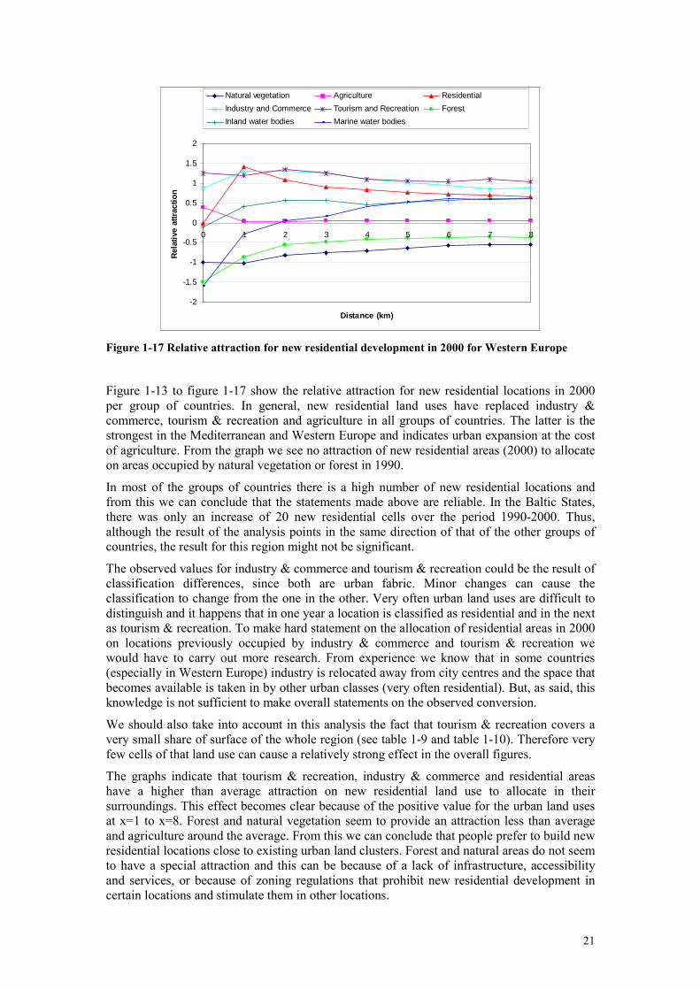
Figure 1-25 Relative attraction for new forest areas in 2000 for South-eastern Europe

-4

-3

-2

-1

0

1

2

0 1 2 3 4 5 6 7 8

Distance (km)

Rel

ativ

e at

trac

tio

n




Figure 1-26 Relative attraction for new forest areas in 2000 for Mediterranean

27

-3

-2

-1

0

1

2

3

4

0 1 2 3 4 5 6 7 8

Distance (km)

Rel

ativ

e_at

trac

tio

n




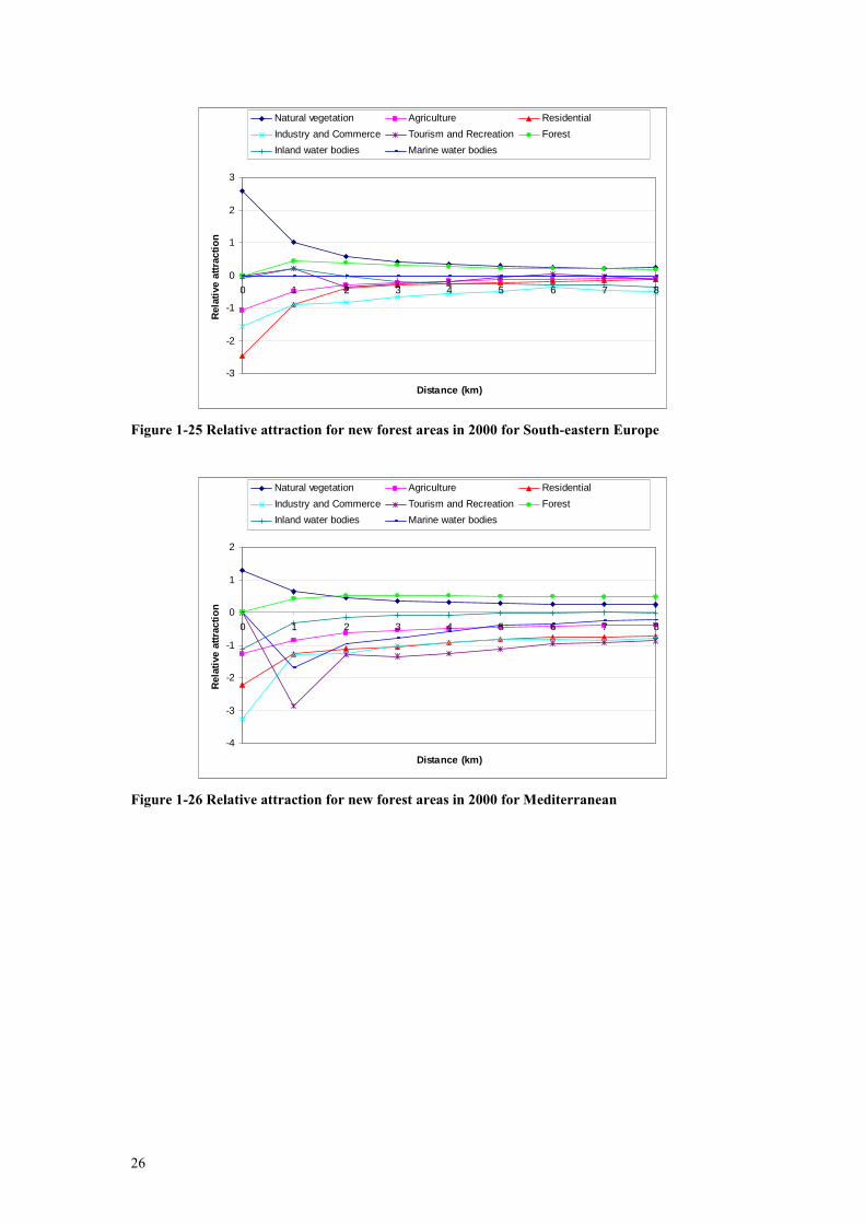
Figure 1-27 Relative attraction for new forest areas in 2000 for Western Europe

Figure 1-23 to figure 1-27 show the relative attraction for new forest in 2000 per group of countries. We see that new forests often take in locations previously occupied by natural vegetation. Generally speaking, we do not see forest appear in 2000 on cell occupied by urban classes in 1990.

At a small distance (from 1 kilometre onwards), natural vegetation and forest were more attractive than average. Residential, industry & commerce and agriculture were less attractive than the average one. Agriculture was about the average attraction. Tourism & recreation was around the average attraction except for in Mediterranean. That’s because the surface share of tourism & recreation of total region in Mediterranean was very small which causes small deviations to stand out. As for forest we can conclude from this that new forest appears on locations that are far from urban areas. Mainly existing forest areas grow, rather than new ones appearing.

Disappeared agriculture in 2000 and its surroundings in 1990

-2.5

-2

-1.5

-1

-0.5

0

0.5

1

0 1 2 3 4 5 6 7 8

Distance (km)

Rel

ativ

e re

pu

lsio

n




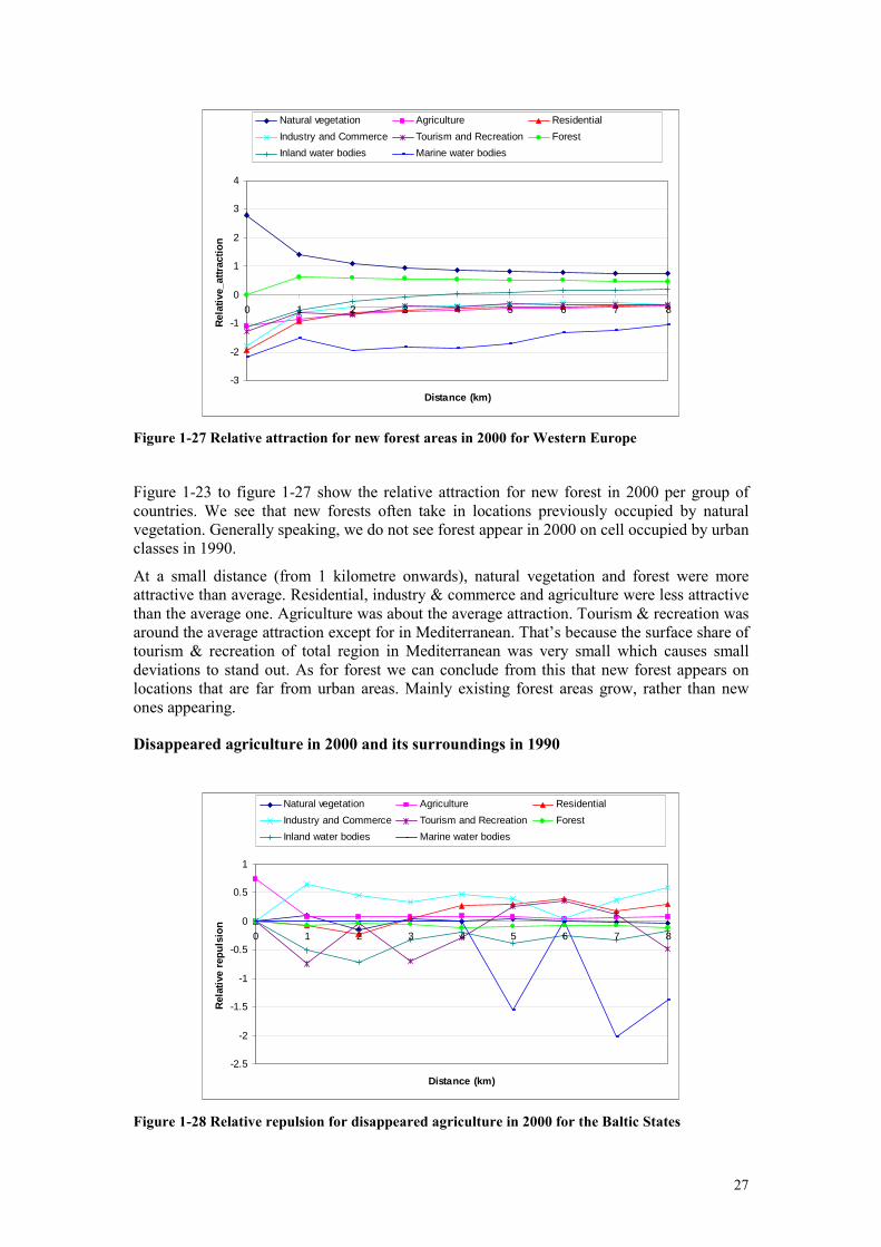
Figure 1-28 Relative repulsion for disappeared agriculture in 2000 for the Baltic States

28

-1.5

-1

-0.5

0

0.5

1

1.5

0 1 2 3 4 5 6 7 8

Distance (km)

Rel

ativ

e re

pu

lsio

n




Figure 1-29 Relative repulsion for disappeared agriculture in 2000 for North-eastern Europe

-4

-3

-2

-1

0

1

2

0 1 2 3 4 5 6 7 8

Distance (km)

Rel

ativ

e re

pu

lsio

n




Figure 1-30 Relative repulsion for disappeared agriculture in 2000 for South-eastern Europe

29

-1

-0.5

0

0.5

1

1.5

2

0 1 2 3 4 5 6 7 8

Distance (km)

Rel

ativ

e re

pu

lsio

n




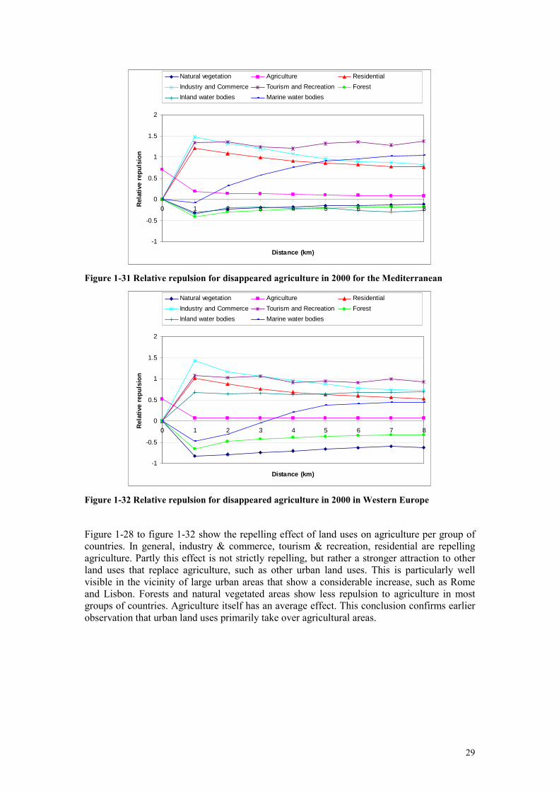
Figure 1-31 Relative repulsion for disappeared agriculture in 2000 for the Mediterranean

-1

-0.5

0

0.5

1

1.5

2

0 1 2 3 4 5 6 7 8

Distance (km)

Rel

ativ

e re

pu

lsio

n




Figure 1-32 Relative repulsion for disappeared agriculture in 2000 in Western Europe

Figure 1-28 to figure 1-32 show the repelling effect of land uses on agriculture per group of countries. In general, industry & commerce, tourism & recreation, residential are repelling agriculture. Partly this effect is not strictly repelling, but rather a stronger attraction to other land uses that replace agriculture, such as other urban land uses. This is particularly well visible in the vicinity of large urban areas that show a considerable increase, such as Rome and Lisbon. Forests and natural vegetated areas show less repulsion to agriculture in most groups of countries. Agriculture itself has an average effect. This conclusion confirms earlier observation that urban land uses primarily take over agricultural areas.

30

Disappeared forest in 2000 and its surroundings in 1990

-5

-4

-3

-2

-1

0

1

2

0 1 2 3 4 5 6 7 8

Distance (km)

Rel

ativ

e re

pu

lsio

n




Figure 1-33 Relative repulsion for disappeared forest in 2000 for the Baltic States

-1.5

-1

-0.5

0

0.5

1

1.5

2

0 1 2 3 4 5 6 7 8

Distance (km)

Rel

ativ

e re

pu

lsio

n




Figure 1-34 Relative repulsion for disappeared forest in 2000 for North-eastern Europe

31

-5

-4

-3

-2

-1

0

1

2

0 1 2 3 4 5 6 7 8

Distance (km)

Rel

ativ

e re

pu

lsio

n




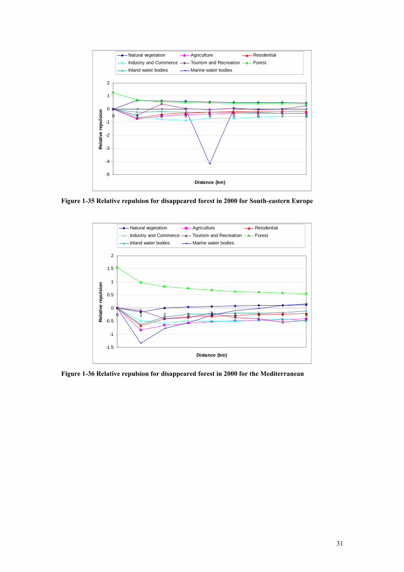
Figure 1-35 Relative repulsion for disappeared forest in 2000 for South-eastern Europe

-1.5

-1

-0.5

0

0.5

1

1.5

2

0 1 2 3 4 5 6 7 8

Distance (km)

Rel

ativ

e re

pu

lsio

n




Figure 1-36 Relative repulsion for disappeared forest in 2000 for the Mediterranean

32

-2

-1.5

-1

-0.5

0

0.5

1

1.5

0 1 2 3 4 5 6 7 8

Distance (kml)

Rel

ativ

e re

pu

lsio

n




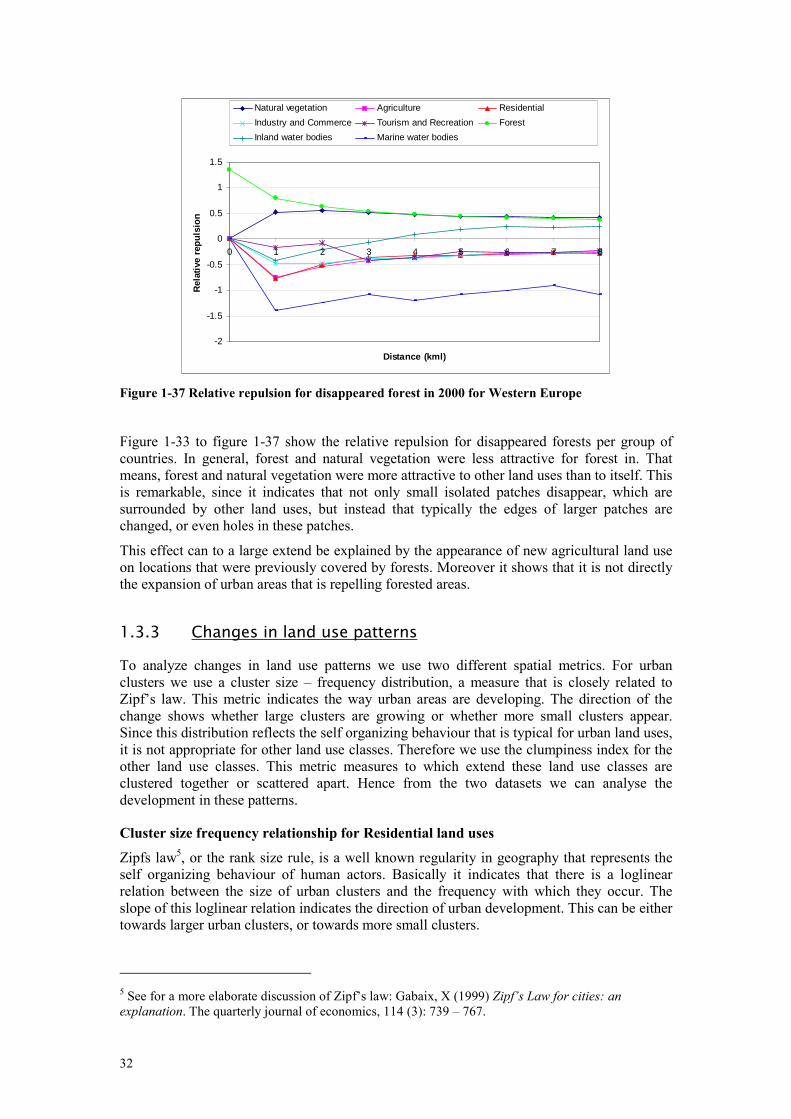
Figure 1-37 Relative repulsion for disappeared forest in 2000 for Western Europe

Figure 1-33 to figure 1-37 show the relative repulsion for disappeared forests per group of countries. In general, forest and natural vegetation were less attractive for forest in. That means, forest and natural vegetation were more attractive to other land uses than to itself. This is remarkable, since it indicates that not only small isolated patches disappear, which are surrounded by other land uses, but instead that typically the edges of larger patches are changed, or even holes in these patches.

This effect can to a large extend be explained by the appearance of new agricultural land use on locations that were previously covered by forests. Moreover it shows that it is not directly the expansion of urban areas that is repelling forested areas.

1.3.3 Changes in land use patterns

To analyze changes in land use patterns we use two different spatial metrics. For urban clusters we use a cluster size – frequency distribution, a measure that is closely related to Zipf’s law. This metric indicates the way urban areas are developing. The direction of the change shows whether large clusters are growing or whether more small clusters appear. Since this distribution reflects the self organizing behaviour that is typical for urban land uses, it is not appropriate for other land use classes. Therefore we use the clumpiness index for the other land use classes. This metric measures to which extend these land use classes are clustered together or scattered apart. Hence from the two datasets we can analyse the development in these patterns.

Cluster size frequency relationship for Residential land uses

Zipfs law5, or the rank size rule, is a well known regularity in geography that represents the self organizing behaviour of human actors. Basically it indicates that there is a loglinear relation between the size of urban clusters and the frequency with which they occur. The slope of this loglinear relation indicates the direction of urban development. This can be either towards larger urban clusters, or towards more small clusters.

5 See for a more elaborate discussion of Zipf’s law: Gabaix, X (1999) Zipf’s Law for cities: an explanation. The quarterly journal of economics, 114 (3): 739 – 767.

33

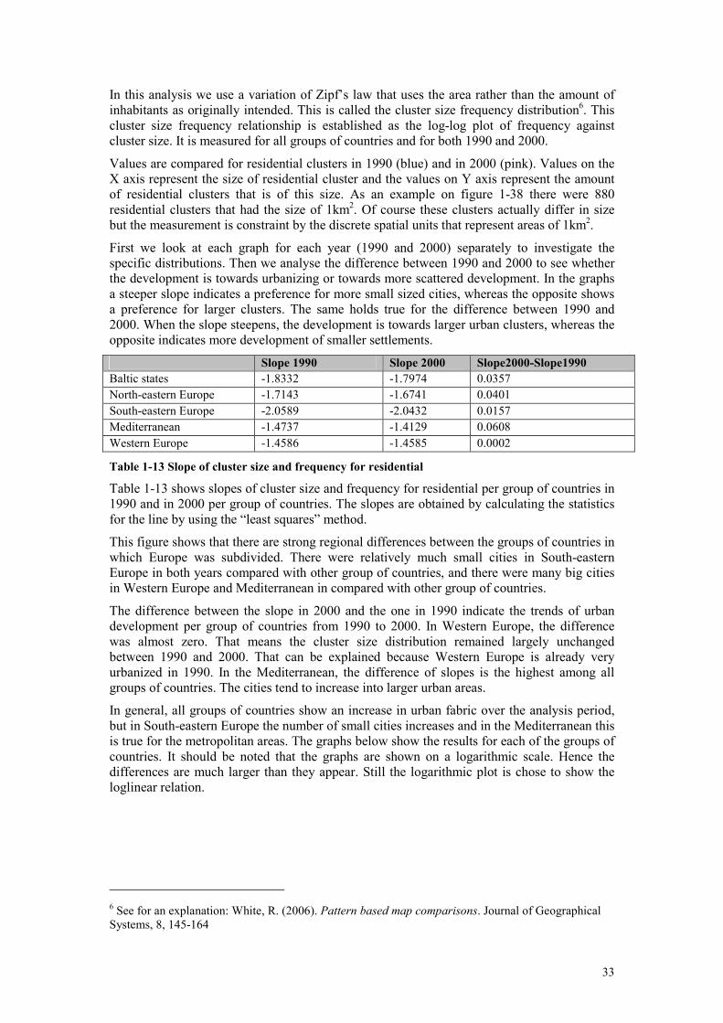
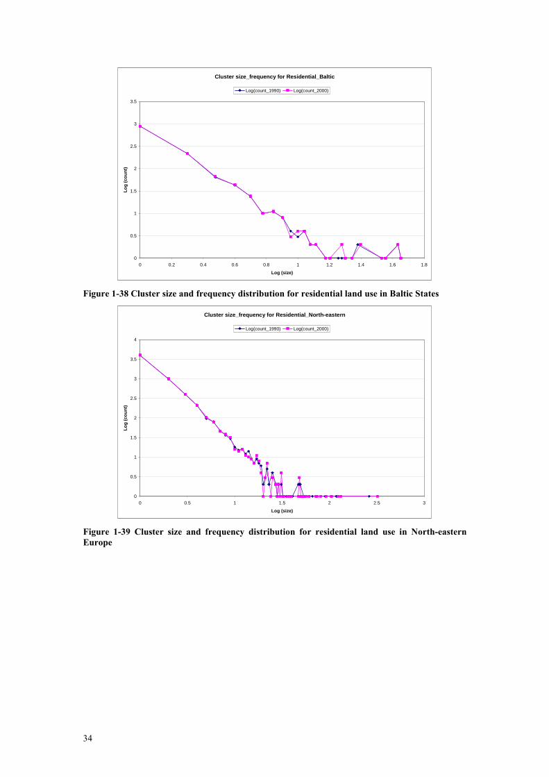
In this analysis we use a variation of Zipf’s law that uses the area rather than the amount of inhabitants as originally intended. This is called the cluster size frequency distribution6. This cluster size frequency relationship is established as the log-log plot of frequency against cluster size. It is measured for all groups of countries and for both 1990 and 2000.

Values are compared for residential clusters in 1990 (blue) and in 2000 (pink). Values on the X axis represent the size of residential cluster and the values on Y axis represent the amount of residential clusters that is of this size. As an example on figure 1-38 there were 880 residential clusters that had the size of 1km2. Of course these clusters actually differ in size but the measurement is constraint by the discrete spatial units that represent areas of 1km2.

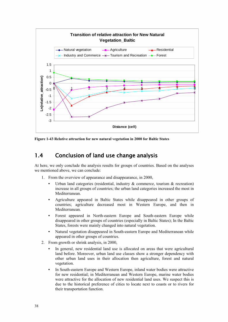
First we look at each graph for each year (1990 and 2000) separately to investigate the specific distributions. Then we analyse the difference between 1990 and 2000 to see whether the development is towards urbanizing or towards more scattered development. In the graphs a steeper slope indicates a preference for more small sized cities, whereas the opposite shows a preference for larger clusters. The same holds true for the difference between 1990 and 2000. When the slope steepens, the development is towards larger urban clusters, whereas the opposite indicates more development of smaller settlements.

Slope 1990 Slope 2000 Slope2000-Slope1990

Baltic states -1.8332 -1.7974 0.0357 North-eastern Europe -1.7143 -1.6741 0.0401 South-eastern Europe -2.0589 -2.0432 0.0157 Mediterranean -1.4737 -1.4129 0.0608 Western Europe -1.4586 -1.4585 0.0002

Table 1-13 Slope of cluster size and frequency for residential

Table 1-13 shows slopes of cluster size and frequency for residential per group of countries in 1990 and in 2000 per group of countries. The slopes are obtained by calculating the statistics for the line by using the “least squares” method.

This figure shows that there are strong regional differences between the groups of countries in which Europe was subdivided. There were relatively much small cities in South-eastern Europe in both years compared with other group of countries, and there were many big cities in Western Europe and Mediterranean in compared with other group of countries.

The difference between the slope in 2000 and the one in 1990 indicate the trends of urban development per group of countries from 1990 to 2000. In Western Europe, the difference was almost zero. That means the cluster size distribution remained largely unchanged between 1990 and 2000. That can be explained because Western Europe is already very urbanized in 1990. In the Mediterranean, the difference of slopes is the highest among all groups of countries. The cities tend to increase into larger urban areas.

In general, all groups of countries show an increase in urban fabric over the analysis period, but in South-eastern Europe the number of small cities increases and in the Mediterranean this is true for the metropolitan areas. The graphs below show the results for each of the groups of countries. It should be noted that the graphs are shown on a logarithmic scale. Hence the differences are much larger than they appear. Still the logarithmic plot is chose to show the loglinear relation.

6 See for an explanation: White, R. (2006). Pattern based map comparisons. Journal of Geographical Systems, 8, 145-164

34

Cluster size_frequency for Residential_Baltic

0

0.5

1

1.5

2

2.5

3

3.5

0 0.2 0.4 0.6 0.8 1 1.2 1.4 1.6 1.8

Log (size)

Lo

g (

cou

nt)

Log(count_1990) Log(count_2000)

Figure 1-38 Cluster size and frequency distribution for residential land use in Baltic States

Cluster size_frequency for Residential_North-eastern

0

0.5

1

1.5

2

2.5

3

3.5

4

0 0.5 1 1.5 2 2.5 3

Log (size)

Lo

g (

cou

nt)


Figure 1-39 Cluster size and frequency distribution for residential land use in North-eastern

Europe

35

Cluster size_frequency for Residential_South-eastern

0

0.5

1

1.5

2

2.5

3

3.5

4

0 0.5 1 1.5 2 2.5

Log (size)

Lo

g (

cou

nt)


Figure 1-40 Cluster size and frequency distribution for residential land use in South-eastern

Europe

Cluster size_frequency for Residential_Mediterranean

0

0.5

1

1.5

2

2.5

3

3.5

4

0 0.5 1 1.5 2 2.5 3

Log (size)

Lo

g (

cou

nt)


Figure 1-41 Cluster size and frequency distribution for residential land use in the Mediterranean

36

Cluster size_frequency for Residential_Western

0

0.5

1

1.5

2

2.5

3

3.5

4

4.5

0 0.5 1 1.5 2 2.5 3 3.5

Log (size)

Lo

g (

cou

nt)


Figure 1-42 Cluster size and frequency distribution for residential land use in Western Europe

Analysis of the clumpiness index for landscape patterns

The clumpiness index was used to analyse the characteristics and changes in landscape patterns. Although the results were measured for several land use categories, the analysis mainly focuses on the natural and agricultural land uses. Those classes are of prime importance in this study, and dynamics in residential patterns are already evaluated with the cluster size frequency distribution.

Clumpiness index is calculated from the adjacency matrix, which shows the frequency with which different types of patches (including like adjacencies between the same patch types) appear side-by-side on the map. Specifically, the clumpiness index expresses the degree to which cells of the same land use type are bordering each other. Clumpiness equals -1 when the focal patch type (i.e. land use class) is maximally disaggregated; Clumpiness equals 0 when the focal patch type is distributed randomly, and Clumpiness equals 1 when the patch type is maximally aggregated (i.e. when all calls of one land use type are connected in one single large patch).

First of all we analyze the clumpiness for natural categories (forest and agriculture) per group of countries. The results of clumpiness analysis for urban categories (residential, industry & commerce, tourism & recreation) are available per group of countries as well (see table 1-14). Larger values for the clumpiness index show that the patches of this specific land use is more compact. The difference of clumpiness of CLC2000 and CLC1990 shows the trend of change of patch for that land use type. If the difference is positive, it means that patches of this specific land use became more compact between 1990 and 2000. Otherwise, the patches of this specific land use are less compact in 2000 than in 1990.

Table 1-14 shows residential land use became more compact in 2000 than in 1990 for all groups of countries. That shows again the cities trended to urbanize development for all groups of countries. We derived the same conclusion from the analysis of cluster size and frequency for residential in previous section. Industry & commerce became more compact in 2000 for most groups of countries except for in Baltic States which have very slight decreased value. Agriculture became less compact in 2000 in most groups of countries except for in North-eastern Europe. Agriculture in North-eastern Europe has the highest relative share of surface among other land uses. The agriculture areas were decreased in 2000 but agriculture clusters itself grew bigger (table 1-14). We can interpret that at the border of agriculture and other urban land categories, some small agricultural patches disappeared and were taken over

37

by other urban land uses in 2000 (figure 1-29). Forest became more compact in 2000 for most groups of countries except for Baltic States because in general, the forest areas were decreased a lot in this region in 2000. Some forest locations became natural vegetation in 2000 after cutting forested areas. Natural vegetation was on top of these forest locations (figure 1-43). It caused the forest patch becoming less compact in 2000.

Region Land use Clumpiness

CLC1990

Clumpiness

CLC2000

Difference of Clumpiness

CLC2000-CLC1990

Baltic States Agriculture 0.4801 0.4784 -0.0017 North-eastern Europe Agriculture 0.5200 0.5207 0.0006 South-eastern Europe Agriculture 0.5689 0.5682 -0.0006 Mediterranean Agriculture 0.6273 0.6249 -0.0024 Western Europe Agriculture 0.5577 0.5535 -0.0042 Baltic States Forest 0.4260 0.4029 -0.0231 North-eastern Europe Forest 0.5318 0.5321 0.0003 South-eastern Europe Forest 0.6199 0.6203 0.0004 Mediterranean Forest 0.5641 0.5651 0.0010 Western Europe Forest 0.5311 0.5323 0.0012 Baltic States Natural vegetation 0.1877 0.1829 -0.0048 North-eastern Europe Natural vegetation 0.3201 0.3806 0.0605 South-eastern Europe Natural vegetation 0.3756 0.3824 0.0068 Mediterranean Natural vegetation 0.5214 0.5200 -0.0014 Western Europe Natural vegetation 0.4881 0.4844 -0.0038 Baltic States Industry & Commerce 0.1906 0.1905 -0.0001 North-eastern Europe Industry & Commerce 0.2040 0.2080 0.0040 South-eastern Europe Industry & Commerce 0.1752 0.1787 0.0035 Mediterranean Industry & Commerce 0.2139 0.2195 0.0056 Western Europe Industry & Commerce 0.2044 0.2079 0.0035 Baltic States Residential 0.2576 0.2583 0.0007 North-eastern Europe Residential 0.2759 0.2786 0.0027 South-eastern Europe Residential 0.2117 0.2124 0.0006 Mediterranean Residential 0.3257 0.3342 0.0085 Western Europe Residential 0.3418 0.3442 0.0024 Baltic States Tourism & Recreation 0.2496 0.2484 -0.0012 North-eastern Europe Tourism & Recreation 0.1644 0.1683 0.0039 South-eastern Europe Tourism & Recreation 0.1846 0.1861 0.0015 Mediterranean Tourism & Recreation 0.1894 0.1792 -0.0102 Western Europe Tourism & Recreation 0.1647 0.1623 -0.0024

Table 1-14 Clumpiness index of CLC in 2000 and in 1990 and its difference

38

Transition of relative attraction for New Natural Vegetation_Baltic

-3

-2.5

-2

-1.5

-1

-0.5

0

0.5

1

1.5

0 1 2 3 4 5 6 7 8

Distance (cell)

Ln

(rel

ativ

e_at

trac

tio

n)



Figure 1-43 Relative attraction for new natural vegetation in 2000 for Baltic States

1.41.41.41.4 Conclusion of land use change analysisConclusion of land use change analysisConclusion of land use change analysisConclusion of land use change analysis

At here, we only conclude the analysis results for groups of countries. Based on the analyses we mentioned above, we can conclude:

1. From the overview of appearance and disappearance, in 2000,

• Urban land categories (residential, industry & commerce, tourism & recreation) increase in all groups of countries; the urban land categories increased the most in Mediterranean.

• Agriculture appeared in Baltic States while disappeared in other groups of countries; agriculture decreased most in Western Europe, and then in Mediterranean.

• Forest appeared in North-eastern Europe and South-eastern Europe while disappeared in other groups of countries (especially in Baltic States); In the Baltic States, forests were mainly changed into natural vegetation.

• Natural vegetation disappeared in South-eastern Europe and Mediterranean while appeared in other groups of countries.

2. From growth or shrink analysis, in 2000,

• In general, new residential land use is allocated on areas that were agricultural land before. Moreover, urban land use classes show a stronger dependency with other urban land uses in their allocation then agriculture, forest and natural vegetation.

• In South-eastern Europe and Western Europe, inland water bodies were attractive for new residential; in Mediterranean and Western Europe, marine water bodies were attractive for the allocation of new residential land uses. We suspect this is due to the historical preference of cities to locate next to coasts or to rivers for their transportation function.

39

• New agriculture mainly appears on top of natural vegetation and forests in most areas. Moreover, agriculture is hardly, if at all attracted to urban land use functions. Instead it is attracted by forest and natural vegetation. This is probably for the availability of land; still it is remarkable since it is opposite to what neo classical economists predict as a result of transport costs to a central market. Agricultural areas close to cities again are often taken over by suburbanization.

• New forest was mainly found on locations with natural vegetation for all regions. Also new forested area are attracted to existing forested an natural land uses, than other land uses, which indicates that existing natural areas and forests are growing rather than new ones appearing.

3. Cluster size analysis in 1990 and in 2000,

• Although the log linear relation between city sizes and the frequency with which they occur is clearly apparent in all country groups, the actual distribution differs considerably among regions. South-eastern Europe shows an abundance of small sized cities, while both Western Europe and the Mediterranean are skewed towards the larger urban areas.

• The log linear relation was preserved over time, when measured from 1990 and 2000; however, the regions show a development towards larger urban centers. This is indicated by the positive change in slope in the cluster size frequency distribution over time (see Table 1-13).

• The exception to this is Western Europe, where the distribution remains largely constant, probably since this area is already very urbanized by 1990 compared to the other country groups. At the other hand, even though the Mediterranean was already heavily inclined towards larger metropolitan areas too, this preference increased over time from 1990 to 2000.

• From the analysis of the land use patterns by means of the clumpiness analysis we can say that urban land use became more compact over time in all areas.

• Patches of forest show the same trend, since they also became more compact over time, except for the Baltic States. The latter can be explained by the clear cutting that takes place there to allocate new agricultural areas. At the other hand, agriculture shows an opposite trend, since the distribution thereof became more scattered over time.

Based on the characteristics that we found in the land use patterns as well as the developments over time, we propose to further cluster the Baltic States and North Eastern Europe together in one application for the calibration of the land use model. The strongest reason for this is the similarity among the neighbourhood relations that we found from the NEIGHBOURHOOD

ANALYSIS TOOL, even though the absolute changes are not. For the scenario analysis part, an additional group of countries is added, Scandinavia. Since land use data was only available for one point in time, this application could not be calibrated on its own however. Therefore we need to make some assumptions on which parameter settings would fit best to this area.

We did not combine Mediterranean and Western Europe even though their neighbourhood relations are similar because the urbanization pattern in Western Europe remains constant while in this is not the case in the Mediterranean. Here cities tend to urbanize further. We leave South-eastern Europe as a separate region because some of its neighbourhood characteristics are different from other groups. Moreover their urbanization pattern is somewhat different from other regions.

41

2.2.2.2. The METRONAMICA modelThe METRONAMICA modelThe METRONAMICA modelThe METRONAMICA model

The most important drivers for land use dynamics seem similar over different geographic locations and different periods in time. However, this is only mostly true on an abstract level and less so the more specific the scope gets. It is widely acknowledged that neighbouring land use is an important driver for the allocation of new urban activities. Still, a closer look at this topic shows that there are vast differences between the clustering of urban land uses in different regions. This is also something we have observed during the historic analysis described in the previous chapter.

This indicates that a general framework that incorporates the main drivers for land use dynamics is perfectly feasible, since main drivers and processes are similar. On the other hand, each application within such a framework needs to be calibrated to the specific dynamics of the location and period. Possible differences between areas are also reflected in the resolution on which they are modelled. On a coarser scale, land use dynamics can be similar, while a more detailed look at finer scales actually shows differences in the exact allocation, reflecting differences in the underlying processes. From a modellers point of view the challenge therefore increases with a resolution and improved data quality. Although the model structure and the drivers incorporated in the system are generic, the actual challenge is to apply the system successfully.

METRONAMICA is a modelling framework supporting the development and application of spatially-dynamic land use models enabling the exploration of spatial developments in cities,

Figure 2-1 The Dutch application of the METRONAMICA modelling framework, the

Environment Explorer, working at 3 spatial levels.

42

regions or countries caused by autonomous developments, external factors, and policy measures using structured ‘what-if analysis’ (RIKS, 2005). The consequences of trends, shocks and policy interventions are visualised by means of dynamic ‘year-by-year’ land use maps as well as spatially explicit economic, ecologic and socio-psychological indicators represented at high spatial resolution. It thus stimulates and facilitates awareness building, learning, and discussion prior to decision-making.

METRONAMICA features a layered model structure representing processes operating at three embedded geographical levels: the global (1 administrative or physical entity), the regional (n administrative or physical entities within the global level) and the local (N cellular units within each regional entity) (see figure 2.2).

At the global level growth figures for the overall population, the activity per economic sector, and the expansion of particular natural land uses are entered in the model as global trend lines.

At the regional level a dynamic spatial interaction based model (see for example: White, 1977, 1978) caters for the fact that the national growth will not evenly spread over the modelled area, rather that regional inequalities will influence the location and relocation of new residents and new economic activity and thus drive regional development. The regional model allocates national growth as well as the interregional migration of activities and residents based on the relative attractiveness of each region.

Subsequently, at the local level, the regional demands are allocated on the land use map by means of a cellular automata based land use allocation model evolving on a grid varying between ¼ha and 4km2 (Couclelis, 1985; White and Engelen, 1993, 1997; Engelen et al., 1995). To simulate land use dynamics, the modelled area is represented as a mosaic of grid cells. Each cell has a cell state that represents its predominant land use and together the cells constitute the changing land use pattern of the region. In principle, it is the relative attractiveness of a cell as viewed by a particular spatial agent, as well as the local constraints and opportunities that cause cells to change from one type of land use to another. Changes in land use at the local level are driven by four important factors (see Figure below):

Time LoopTime LoopTime LoopTime LoopTime LoopTime LoopTime LoopTime Loop1. Suitability

2. Zoning

Transition potential

Land use

4. Land use & CA-rules

&&

&

= =>

3. Accessibility

Time LoopTime LoopTime LoopTime LoopTime LoopTime LoopTime LoopTime Loop1. Suitability1. Suitability

2. Zoning2. Zoning



Land useLand use



&&

&

= =>

3. Accessibility

43

• Physical suitability, represented by one map per land use function modelled. The term suitability is used here to describe the degree to which a cell is fit to support a particular land use function and the associated economic or residential activity for a particular activity.

• Zoning or institutional suitability, represented by one map per land use function modelled. For different planning periods the map specifies which cells can and cannot be taken in by the particular land use.

• Accessibility, represented by one map per land use function modelled. Accessibility is an expression of the ease with which an activity can fulfil its needs for transportation and mobility in a particular cell based on the transportation system

• Dynamic interaction of land uses in the area immediately surrounding a location is represented by the land use and the Cellular Automata (CA) rules. For each land use function, a set of spatial interaction rules determines the degree to which it is attracted to, or repelled by, the other functions present in its surroundings; a 196 cell neighbourhood. If the attractiveness is high enough, the function will try to occupy the location, if not, it will look for more attractive places. New activities and land uses invading a neighbourhood over time will thus change its attractiveness for activities already present and others searching for space. This process constitutes the highly non-linear character of this model.

On the basis of these four elements, the model calculates for every simulation step the transition potential for each cell and function. In the course of time and until regional demands are satisfied, cells will change to the land use function for which they have the highest transition potential. Consequently, the transition potentials reflect the pressures exerted on the land and thus constitute important information for those responsible for the design of sound spatial planning policies. For the application of METRONAMICA in the current project we have omitted the regional layer because socio-economic demands at NUTS 2 region were provided by our partner TERSYN.

To calibrate a METRONAMICA application, one needs to adjust parameter values to improve the models’ fit. This is not an easy task, since the proposed model contains a multitude of parameters that influence the eventual result - and each other. Moreover –as stated above– this calibration is region-specific since each region has its own particularities when it comes to land use dynamics and it takes time to analyze these particularities and parameterize them. Main parameters that need calibration are the interaction rules, the extent of the random effect, the accessibility parameters and the weighing factors for the suitability and the different element in the total potential. The calibration procedure and results are discussed in the next chapter.

On of the difficulties in calibration in general, is the availability of long time series of consistent data sets. Since land use changes occur over relatively long periods, deriving relations of land use change based on a ten year period is a real challenge. However, the better the land use model is able to actually capture the process of land use change, the more the data can be used as a verification and fine-tuning of the process and its parameters, rather than as a way of understanding the process of land use change. For this reason we propose to use a process-based land use model and use the calibration to fine-tune the parameters and relations in this model.

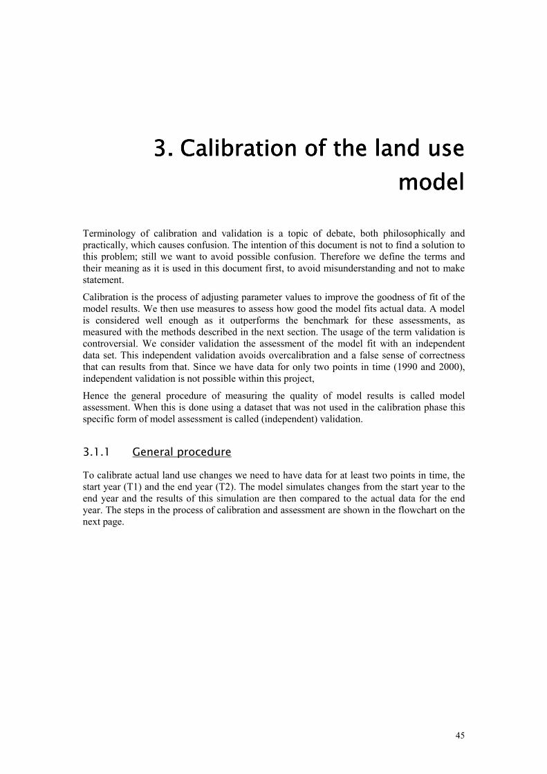
45

3.3.3.3. CCCCalibration of the land use alibration of the land use alibration of the land use alibration of the land use

modelmodelmodelmodel

Terminology of calibration and validation is a topic of debate, both philosophically and practically, which causes confusion. The intention of this document is not to find a solution to this problem; still we want to avoid possible confusion. Therefore we define the terms and their meaning as it is used in this document first, to avoid misunderstanding and not to make statement.

Calibration is the process of adjusting parameter values to improve the goodness of fit of the model results. We then use measures to assess how good the model fits actual data. A model is considered well enough as it outperforms the benchmark for these assessments, as measured with the methods described in the next section. The usage of the term validation is controversial. We consider validation the assessment of the model fit with an independent data set. This independent validation avoids overcalibration and a false sense of correctness that can results from that. Since we have data for only two points in time (1990 and 2000), independent validation is not possible within this project,

Hence the general procedure of measuring the quality of model results is called model assessment. When this is done using a dataset that was not used in the calibration phase this specific form of model assessment is called (independent) validation.

3.1.1 General procedure

To calibrate actual land use changes we need to have data for at least two points in time, the start year (T1) and the end year (T2). The model simulates changes from the start year to the end year and the results of this simulation are then compared to the actual data for the end year. The steps in the process of calibration and assessment are shown in the flowchart on the next page.

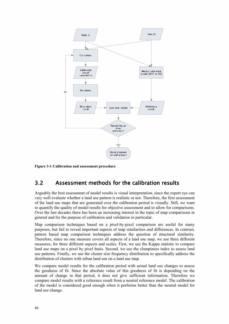
46

Figure 3-1 Calibration and assessment procedure

3.23.23.23.2 Assessment methods for the calibration resultsAssessment methods for the calibration resultsAssessment methods for the calibration resultsAssessment methods for the calibration results

Arguably the best assessment of model results is visual interpretation, since the expert eye can very well evaluate whether a land use pattern is realistic or not. Therefore, the first assessment of the land use maps that are generated over the calibration period is visually. Still, we want to quantify the quality of model results for objective assessment and to allow for comparisons. Over the last decades there has been an increasing interest in the topic of map comparisons in general and for the purpose of calibration and validation in particular.

Map comparison techniques based on a pixel-by-pixel comparison are useful for many purposes, but fail to reveal important aspects of map similarities and differences. In contrast, pattern based map comparison techniques address the question of structural similarity. Therefore, since no one measure covers all aspects of a land use map, we use three different measures, for three different aspects and scales. First, we use the Kappa statistic to compare land use maps on a pixel by pixel basis. Second, we use the clumpiness index to assess land use patterns. Finally, we use the cluster size frequency distribution to specifically address the distribution of clusters with urban land use on a land use map.

We compare model results for the calibration period with actual land use changes to assess the goodness of fit. Since the absolute value of this goodness of fit is depending on the amount of change in that period, it does not give sufficient information. Therefore we compare model results with a reference result from a neutral reference model. The calibration of the model is considered good enough when it performs better than the neutral model for land use change.

47

3.2.1 Neutral reference model for land use changes

As a reference model for land use changes we use the random constraint match. A more elaborate explanation of the use of this method can be found in Hagen-Zanker and Lajoie (2008). The Random Constraint Match model creates a new map by minimally adjusting the initial map to obtain the same composition as the final map. The model first assesses for all classes by how many cells they are under- or overrepresented in the initial map relative to the final map. For each class that is overrepresented it will select randomly the surplus cells on the initial map. I.e. if in the initial map there are 450 cells of urban and on the final map there are 410, the class urban is overrepresented by 40 cells and out of the 450 cells of urban 40 will be selected to change class.

Then, the underrepresented classes are distributed randomly over the selected cells on the initial map. I.e. if in the earlier step 230 cells have been selected, of which 40 were originally urban, and the class agriculture is underrepresented by 60 cells then out of the 230 cells, 60 will be selected to become agriculture. After all cells have been distributed, the modified initial map is the result of the Random Constraint Model. Measurements obtained from the map that was generated with the random constraint match are indicated with RCM.

3.2.2 Kappa statistics

The Kappa comparison method is based on a straightforward cell-by-cell map comparison, which considers for each pair of cells on the two maps whether they are equal or not. It is defined as the goodness of fit between two categorical maps, corrected for the goodness of fit as can be expected by chance (Congalton, 1991). Values range between -1 and 1, where -1 indicates no agreement at all and 1 indicates a perfect fit. The value 0 indicates an agreement equal to what can be expected by chance.

The Kappa statistic results from two types of similarities, similarity of quantity and similarity of location, where the first refers to the number of cells per category and the second to the location of these cells on the lattice. In order to see where dissimilarities come from, the Kappa statistic is split in two statistics: Kappa Histogram and Kappa Location. For more information see Hagen (2002). All three types of Kappa results can be computed from the MAP COMPARISON KIT..

Kappa statistics for model results are derived by comparing the simulated land use map at the end of a simulation period with the actual land use map for the same year. However, model results often yield high Kappa values (much higher than 0). This is because most land use does not change over time, and therefore most pixels representing land use do not either. Actually the absolute value of Kappa is mostly depending on the amount of land use change over time. Therefore Kappa statistics are only valuable when compared to results obtained from the neutral reference model.

3.2.3 Clumpiness index

The clumpiness index is a moving window based measure that is used to assess the similarity in land use patterns. It is a relative measure that indicates to which extend cells with similar classes are bordering each other. Its values range from -1 to 1, where -1 indicates a minimal connection and 1 indicates a maximum connection to cells with a similar land use.

To assess the clumpiness of simulation results, the average clumpiness per land use class is computed for the whole map, both for the actual land use map in the end year and the simulated land use map in that year. These values are then compared to the results obtained from the random constraint match. The model result is considered good enough if its clumpiness for the different land use classes is closer to the measurements obtain from the

48

data than the random reference maps. Only those land uses that are modelled as functions are assessed. For a more elaborate description of the clumpiness index see McGarigal et al. (2002).

3.2.4 Cluster size – frequency distribution

We use the cluster size frequency distribution as a fractal measure to measure the distribution of sizes for urban clusters. For large areas the distribution of urban cluster sizes shows a remarkable regularity, which appears when the cluster size (measured in a number of pixels) is counted against the number of times this frequency occurs. When drawn on a logarithmic scale a straight line appears which is maintained over time. For a more elaborate discussion, see White (2006).

In calibration we use this regularity to test the long term behaviour of our model. From the initial land use map, the cluster size frequency distribution is measured as a reference. Then the model is run for an extended period in future, say 30 or 50 years with continuous developments for urban growth. From the extended simulation result the cluster size frequency distribution is measured again to verify whether it is maintained over time. Hence we use it to seen that larger clusters grow, but also that new clusters appear. The extended simulation result is compared to the distribution from the start year and the end year for which there is data.

Moreover, from the slope of the start year and the end year you can measure the trend in the development of the urbanization pattern. An increasing slope (more negative) indicates an increase in new smaller clusters, while a decreasing slope (less negative) indicates that larger clusters are growing faster. The trend that is detected over the calibration period should be maintained over the extended simulation period, at least qualitatively.

3.33.33.33.3 Calibration resultsCalibration resultsCalibration resultsCalibration results

As the conclusion, four METRONAMICA applications are set up for the calibration according to the analysis of land use characteristics for groups of countries presented in section 1.4. These groups of countries are (1) the Baltic States and North-eastern Europe, (2) South-eastern Europe, (3) the Mediterranean, and (4) Western Europe.

3.3.1 Data in the CA land use model

The following data was used to set up the application: a land use map for 1990, a land use map for 2000, a map with boundaries of NUTS2 regions, a transport network map, suitability maps per land use function, zoning maps per land use function. The latter two are the result of pre-processing external to the model. The following sections describe the data source and procedure of preparation.

Land use data

The land use data that was used in the calibration is the same that was used for the assessment of historic land use changes. The original data was reclassified and aggregated to a 1 km resolution as described in section 1.2. The CLC 1990 is not available for Cyprus, Finland, Malta, Sweden and United Kingdom. Thus in the calibration procedure, these countries were excluded.

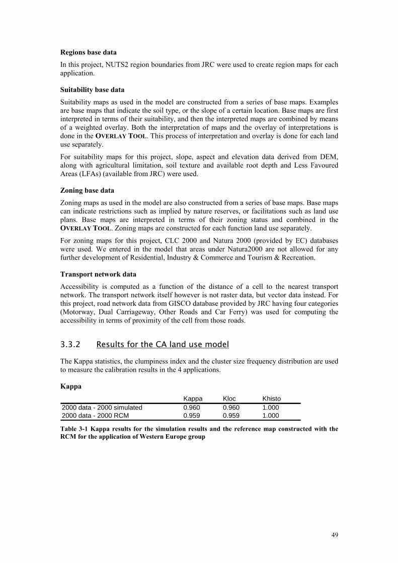
49

Regions base data

In this project, NUTS2 region boundaries from JRC were used to create region maps for each application.

Suitability base data

Suitability maps as used in the model are constructed from a series of base maps. Examples are base maps that indicate the soil type, or the slope of a certain location. Base maps are first interpreted in terms of their suitability, and then the interpreted maps are combined by means of a weighted overlay. Both the interpretation of maps and the overlay of interpretations is done in the OVERLAY TOOL. This process of interpretation and overlay is done for each land use separately.

For suitability maps for this project, slope, aspect and elevation data derived from DEM, along with agricultural limitation, soil texture and available root depth and Less Favoured Areas (LFAs) (available from JRC) were used.

Zoning base data

Zoning maps as used in the model are also constructed from a series of base maps. Base maps can indicate restrictions such as implied by nature reserves, or facilitations such as land use plans. Base maps are interpreted in terms of their zoning status and combined in the OVERLAY TOOL. Zoning maps are constructed for each function land use separately.

For zoning maps for this project, CLC 2000 and Natura 2000 (provided by EC) databases were used. We entered in the model that areas under Natura2000 are not allowed for any further development of Residential, Industry & Commerce and Tourism & Recreation.

Transport network data

Accessibility is computed as a function of the distance of a cell to the nearest transport network. The transport network itself however is not raster data, but vector data instead. For this project, road network data from GISCO database provided by JRC having four categories (Motorway, Dual Carriageway, Other Roads and Car Ferry) was used for computing the accessibility in terms of proximity of the cell from those roads.

3.3.2 Results for the CA land use model

The Kappa statistics, the clumpiness index and the cluster size frequency distribution are used to measure the calibration results in the 4 applications.

Kappa

Kappa Kloc Khisto2000 data - 2000 simulated 0.960 0.960 1.0002000 data - 2000 RCM 0.959 0.959 1.000

Table 3-1 Kappa results for the simulation results and the reference map constructed with the

RCM for the application of Western Europe group

50

Kappa Khisto KlocNatural vegetation 0.851 0.851 1.000Agriculture 0.973 0.973 1.000Residential 0.945 0.945 1.000Industy and Commerce 0.800 0.800 1.000Tourism and Recreation 0.833 0.833 1.000Forest 0.971 0.971 1.000Natural vegetation 0.877 0.877 1.000Agriculture 0.975 0.975 1.000Residential 0.941 0.941 1.000Industy and Commerce 0.791 0.791 1.000Tourism and Recreation 0.828 0.828 1.000Forest 0.974 0.974 1.000

2000 data - 2000 simulated

2000 data - 2000 RCM

Table 3-2 Kappa results per land use category for the simulation results and the reference map

constructed with the RCM for the application of Western Europe group

Clumpiness index

Group Land use 2000 data 2000 simulated 2000 RCMWestern Europe Natural vegetation 0.484 0.468 0.472

Agriculture 0.553 0.553 0.546Residential 0.344 0.363 0.324Industy and Commerce 0.208 0.226 0.163Tourism and Recreation 0.162 0.187 0.139Forest 0.532 0.535 0.531

Mediterranean Natural vegetation 0.520 0.520 0.516Agriculture 0.625 0.625 0.622Residential 0.334 0.356 0.289Industy and Commerce 0.219 0.236 0.162Tourism and Recreation 0.179 0.286 0.136Forest 0.565 0.572 0.564

South-eastern Europe Natural vegetation 0.382 0.383 0.368Agriculture 0.568 0.568 0.566Residential 0.212 0.213 0.211Industy and Commerce 0.179 0.174 0.171Tourism and Recreation 0.186 0.193 0.182Forest 0.620 0.628 0.615

Baltic States and Natural vegetation 0.273 0.256 0.217North-eastern Europe Agriculture 0.515 0.515 0.514

Residential 0.276 0.277 0.269Industy and Commerce 0.202 0.197 0.192Tourism and Recreation 0.182 0.182 0.178Forest 0.494 0.505 0.491

Table 3-3 Clumpiness scores per land use category per group of countries

51

Group Land use |2000simulated - 2000data||2000simulated - 2000RCM|Western Europe Natural vegetation 0.016 0.004

Agriculture 0.000 0.007Residential 0.019 0.039Industry and Commerce 0.097 0.063Tourism and Recreation 0.024 0.048Forest 0.002 0.004

Mediterranean Natural vegetation 0.000 0.004Agriculture 0.000 0.004Residential 0.022 0.068Industry and Commerce 0.053 0.075Tourism and Recreation 0.124 0.149Forest 0.007 0.008

South-eastern Europe Natural vegetation 0.001 0.015Agriculture 0.000 0.003Residential 0.001 0.002Industry and Commerce 0.036 0.003Tourism and Recreation 0.022 0.011Forest 0.008 0.013

Baltic States and Natural vegetation 0.017 0.039North-eastern Europe Agriculture 0.000 0.002

Residential 0.001 0.008Industry and Commerce 0.072 0.005Tourism and Recreation 0.010 0.004Forest 0.010 0.013

Table 3-4 Difference of clumpiness scores per land use category per group of countries

Cluster size – frequency distribution

0

0.5

1

1.5

2

2.5

3

3.5

4

4.5

0 0.5 1 1.5 2 2.5 3 3.5

Log (size)

Lo

g (f

req

uen

cy)

Log(count_1990) Log(count_2000) Log(count_2030)

Figure 3-2 Cluster size-frequency distribution for Western Europe group

52

0

0.5

1

1.5

2

2.5

3

3.5

4

0 0.5 1 1.5 2 2.5 3 3.5

Log (size)

Lo

g (f

req

uen

cy)


Figure 3-3 Cluster size-frequency distribution for Mediterranean group

0

0.5

1

1.5

2

2.5

3

3.5

4

0 0.5 1 1.5 2 2.5

Log (size)

Lo

g (f

req

uen

cy)


Figure 3-4 Cluster size-frequency distribution for South-eastern Europe group

53

0

0.5

1

1.5

2

2.5

3

3.5

4

0 0.5 1 1.5 2 2.5 3

Log (size)

Lo

g (f

req

uen

cy)


Figure 3-5 Cluster size-frequency distribution for Baltic States and North-eastern Europe group

3.43.43.43.4 ConclusionConclusionConclusionConclusion of the of the of the of the calibration calibration calibration calibration results results results results

The Kappa statistics for the calibration period for Western Europe group is given as one example in table 3-1. the results are further subdivided into Khist and Klocation, where Khisto in the RCM result is 1 by definition. The Kappa score for the simulation results is higher than that for the reference map. The results indicate that the calibration of the CA land use model is successful in the sense that the model outperforms the reference map over the calibration period (1990-2000). By applying the Kappa statistics per category it becomes clear that results differ somewhat among land use classes. The table 3-2 shows the Kappa results per land use categories. The Kappa for the simulation results for residential, industry and commerce, tourism and recreation are higher than the ones for the reference map with RCM, respectively which indicates the calibration for these land use categories are successful. The scores for the other land use categories do not show this result. However, when assessing the patterns they look realistic. This indicates that the process as simulated is realistic, but that some exact allocations are missed. We suspect that this can partly be explained by classification issues in the CLC land use maps. Comparison from 1990 to 2000 shows quite some land use changes from natural vegetation to forest and vice versa that can be caused by remote sensing classification rather than actual land use changes.

Table 3-3 shows the clumpiness scores per land use category for the actual land use map per group of countries, the simulated land use map and the reference map. Table 3-4 shows the absolute difference per group of countries between the simulated result and the actual land use, and the difference between the simulated result and the reference result. The difference for most of the land uses between the simulated map and the actual map is smaller than the difference between the simulated map and the reference map. Exceptions occur in the land use classes recreation and industry & commerce in some groups of countries. This can be explained by the fact that there is not much new recreation and industry & commerce occur over the calibration period, which causes a small number of cells to have a considerable

54

effect. Altogether the clumpiness scores indicate that land use patterns are well preserved over the calibration which confirms that the model generates realistic results.

In order to test the long term behaviour of the CA model, the model is run for an extended period in future 40 years, from 1990 until 2030 with continuous developments for urban growth. In order to run the simulation till 2030, the population and GDP for the baseline scenario are used to calculate the land use demand for 2030. Figure 3-2 to figure 3-5 show the cluster size frequency distribution for the residential areas for the year 1990, 2000, and 2030. These figures show the trend of the cluster size frequency distribution detected from 1990 to 2000 is maintained over the extended simulation year 2030.

This figure again indicates that there are clear regional differences between the groups of countries in Europe (see section Cluster size frequency relationship for Residential land uses). In the countries in Western Europe (see figure 3-2) and the Mediterranean (see figure 3-3), the development is towards urbanization, since big cities grow larger. For the other country groups this is not so much the case, and particularly in countries in North-eastern Europe, smaller settlements are developing, as can be seen from figure 3-4.

It should be noted that differences in the graphs appear very small and are therefore hard to detect. This is mainly because of the logarithmic scale that is used to depict the results. What we can mainly conclude from the graph alone is that the cluster size frequency distributions are generally very well maintained over time. This indicates a very realistic urbanization patterns. The conclusions drawn above are based on the numerical values as rather than only the visual interpretation of the map.

55

4.4.4.4. ScenariosScenariosScenariosScenarios

4.14.14.14.1 Applications for scenariosApplications for scenariosApplications for scenariosApplications for scenarios

In order to carry out the scenarios study, five METRONAMICA applications are set up which include Cyprus, Finland, Malta, Sweden and the United Kingdom. Table 4-4 shows the list of group of countries during scenarios study. United Kingdom is in the Western Europe group. Cyprus and Malta are in the Mediterranean group. Finland and Sweden are grouped in the Scandinavia. Since there was no land use data for these countries for 1990 and 2000 they were not calibrated. Therefore we used the same parameter values as found in the Baltic States and North-eastern Europe for the application of Scandinavia.

NUTS-0 Name Group of countries for Scenarios

EE Estonia Baltic states and North-eastern Europe LT Lithuania Baltic states and North-eastern Europe LV Latvia Baltic states and North-eastern Europe CZ Czech Republic Baltic states and North-eastern Europe PL Poland Baltic states and North-eastern Europe SK Slovakia Baltic states and North-eastern Europe BG Bulgaria South-eastern Europe HU Hungary South-eastern Europe RO Romania South-eastern Europe SI Slovenia South-eastern Europe ES Spain Mediterranean GR Greece Mediterranean IT Italy Mediterranean PT Portugal Mediterranean CY Cyprus Mediterranean MT Malta Mediterranean AT Austria Western Europe BE Belgium Western Europe DE Germany Western Europe DK Denmark Western Europe FR France Western Europe IE Ireland Western Europe LU Luxemburg Western Europe NL The Netherlands Western Europe UK United Kingdom Western Europe FI Finland Scandinavia SE Sweden Scandinavia

Table 4-1 Group of countries list for scenarios

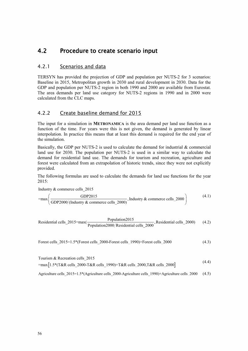
56

4.24.24.24.2 Procedure to create scenario inputProcedure to create scenario inputProcedure to create scenario inputProcedure to create scenario input

4.2.1 Scenarios and data

TERSYN has provided the projection of GDP and population per NUTS-2 for 3 scenarios: Baseline in 2015, Metropolitan growth in 2030 and rural development in 2030. Data for the GDP and population per NUTS-2 region in both 1990 and 2000 are available from Eurostat. The area demands per land use category for NUTS-2 regions in 1990 and in 2000 were calculated from the CLC maps.

4.2.2 Create baseline demand for 2015

The input for a simulation in METRONAMICA is the area demand per land use function as a function of the time. For years were this is not given, the demand is generated by linear interpolation. In practice this means that at least this demand is required for the end year of the simulation.

Basically, the GDP per NUTS-2 is used to calculate the demand for industrial & commercial land use for 2030. The population per NUTS-2 is used in a similar way to calculate the demand for residential land use. The demands for tourism and recreation, agriculture and forest were calculated from an extrapolation of historic trends, since they were not explicitly provided.

The following formulas are used to calculate the demands for land use functions for the year 2015:

Industry & commerce cells_2015

GDP2015=max , Industry & commerce cells_2000

GDP2000 (Industry & commerce cells_2000)

(4.1)

Population2015Residential cells_2015=max( ,Residential cells_2000)

Population2000 Residential cells_2000 (4.2)

Forest cells_2015=1.5*(Forest cells_2000-Forest cells_1990)+Forest cells_2000 (4.3)

[ ]Tourism & Recreation cells_2015

=max 1.5*(T&R cells_2000-T&R cells_1990)+T&R cells_2000,T&R cells_2000 (4.4)

Agriculture cells_2015=1.5*(Agriculture cells_2000-Agriculture cells_1990)+Agriculture cells_2000 (4.5)

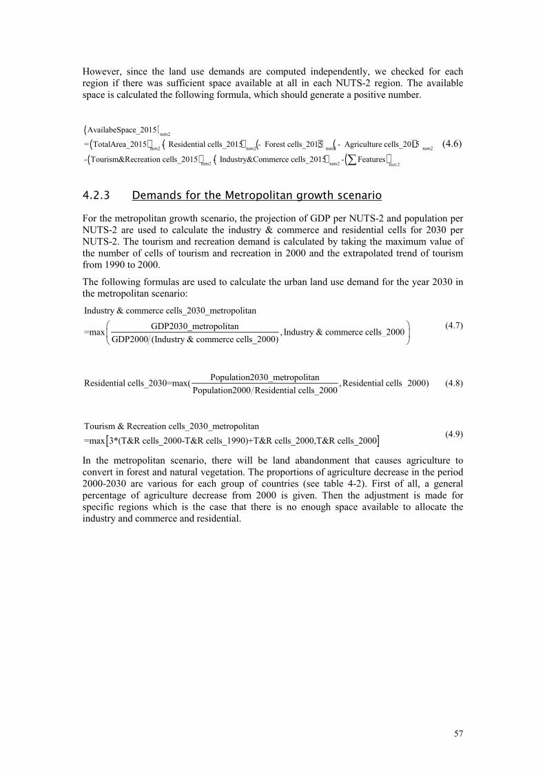
57

However, since the land use demands are computed independently, we checked for each region if there was sufficient space available at all in each NUTS-2 region. The available space is calculated the following formula, which should generate a positive number.

( )( ) ( ) ( ) ( )

( ) ( )

nuts2

nuts2 nuts2 nuts2 nuts2

nuts2 nuts2

AvailabeSpace_2015

= TotalArea_2015 - Residential cells_2015 - Forest cells_2015 - Agriculture cells_2015

- Tourism&Recreation cells_2015 - Industry&Commerce cells_2015 - Features( )2nuts

∑

(4.6)

4.2.3 Demands for the Metropolitan growth scenario

For the metropolitan growth scenario, the projection of GDP per NUTS-2 and population per NUTS-2 are used to calculate the industry & commerce and residential cells for 2030 per NUTS-2. The tourism and recreation demand is calculated by taking the maximum value of the number of cells of tourism and recreation in 2000 and the extrapolated trend of tourism from 1990 to 2000.

The following formulas are used to calculate the urban land use demand for the year 2030 in the metropolitan scenario:

Industry & commerce cells_2030_metropolitan

GDP2030_metropolitan=max , Industry & commerce cells_2000


(4.7)

Population2030_metropolitanResidential cells_2030=max( ,Residential cells_2000)

Population2000 Residential cells_2000 (4.8)

[ ]Tourism & Recreation cells_2030_metropolitan

=max 3*(T&R cells_2000-T&R cells_1990)+T&R cells_2000,T&R cells_2000 (4.9)

In the metropolitan scenario, there will be land abandonment that causes agriculture to convert in forest and natural vegetation. The proportions of agriculture decrease in the period 2000-2030 are various for each group of countries (see table 4-2). First of all, a general percentage of agriculture decrease from 2000 is given. Then the adjustment is made for specific regions which is the case that there is no enough space available to allocate the industry and commerce and residential.

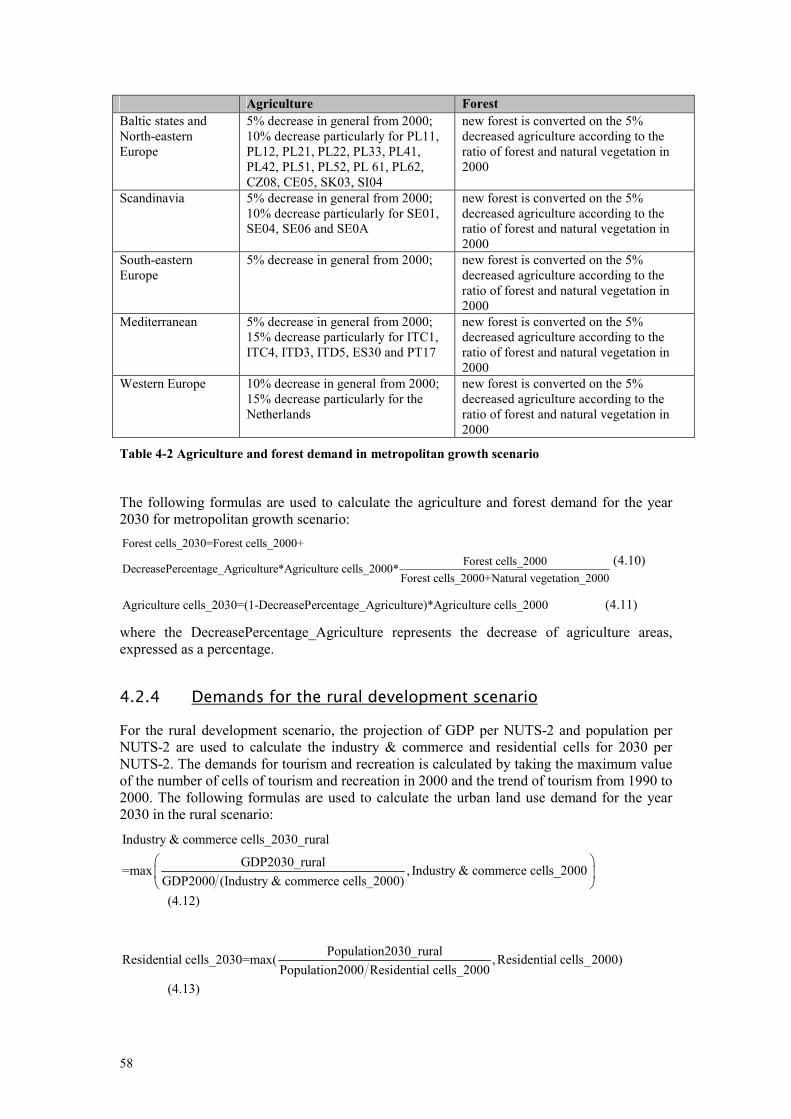
58

Agriculture Forest

Baltic states and North-eastern Europe

5% decrease in general from 2000; 10% decrease particularly for PL11, PL12, PL21, PL22, PL33, PL41, PL42, PL51, PL52, PL 61, PL62, CZ08, CE05, SK03, SI04

new forest is converted on the 5% decreased agriculture according to the ratio of forest and natural vegetation in 2000

Scandinavia 5% decrease in general from 2000; 10% decrease particularly for SE01, SE04, SE06 and SE0A


South-eastern Europe

5% decrease in general from 2000; new forest is converted on the 5% decreased agriculture according to the ratio of forest and natural vegetation in 2000

Mediterranean 5% decrease in general from 2000; 15% decrease particularly for ITC1, ITC4, ITD3, ITD5, ES30 and PT17


Western Europe 10% decrease in general from 2000; 15% decrease particularly for the Netherlands


Table 4-2 Agriculture and forest demand in metropolitan growth scenario

The following formulas are used to calculate the agriculture and forest demand for the year 2030 for metropolitan growth scenario:

Forest cells_2030=Forest cells_2000+

Forest cells_2000DecreasePercentage_Agriculture*Agriculture cells_2000*

Forest cells_2000+Natural vegetation_2000

(4.10)

Agriculture cells_2030=(1-DecreasePercentage_Agriculture)*Agriculture cells_2000 (4.11)

where the DecreasePercentage_Agriculture represents the decrease of agriculture areas, expressed as a percentage.

4.2.4 Demands for the rural development scenario

For the rural development scenario, the projection of GDP per NUTS-2 and population per NUTS-2 are used to calculate the industry & commerce and residential cells for 2030 per NUTS-2. The demands for tourism and recreation is calculated by taking the maximum value of the number of cells of tourism and recreation in 2000 and the trend of tourism from 1990 to 2000. The following formulas are used to calculate the urban land use demand for the year 2030 in the rural scenario:

Industry & commerce cells_2030_rural

GDP2030_rural=max , Industry & commerce cells_2000


(4.12)

Population2030_ruralResidential cells_2030=max( ,Residential cells_2000)

Population2000 Residential cells_2000

(4.13)

59

[ ]Tourism & Recreation cells_2030_rural

=max 3*(T&R cells_2000-T&R cells_1990)+T&R cells_2000,T&R cells_2000

(4.14)

In the rural development scenario, there is an expansion of agricultural areas and forests at the cost of natural vegetation. However, for some regions in this scenario, the land use demands exceed the available space. Therefore, specific adjustments were made for some regions. The amount of change for agriculture and forests in the period 2000-2030 is given for each group of countries in table 4-3.

Agriculture Forest

Baltic states and North-eastern Europe

0.3% increase in general from 2000; 10% decrease particularly for PL11, PL12, PL21, PL22, PL33, PL41, PL42, PL51, PL52, PL 61, PL62, CZ08, CE05, SK03, SI04

0.3% increase from 2000

Scandinavia 0.5% increase in general from 2000; 5% decrease particularly for SE01, SE04, SE06 and SE0A

0.5% increase in general from 2000; constant forest 2000 for SE01, SE04, SE06 and SE0A

South-eastern Europe 5% decrease in general from 2000; constant forest 2000 Mediterranean 2% increase in general from 2000; 10%

decrease particularly for ITC1, ITC4, ITD3, ITD5, ES30 and PT17

0.5% increase in general from 2000; constant forest for ITC1, ITC4, ITD3, ITD5, ES30 and PT17

Western Europe 5% decrease in general from 2000; 15% decrease particularly for the Netherlands; 10% decrease for AT13, BE10, BE21, BE22, BE23, BE24, BE25, BE31, DE30, DE50, DE60, DEA1, DEA2, DEA5, FR10, LU00, UKD3, UKD5, UKI1, UKI2

0.1% increase from 2000

Table 4-3 Agriculture and forest demand in rural development scenario

The following formulas are used to calculate the agriculture and forest demand for the year 2030 for rural development scenario:

Forest cells_2030=(1+ChangePercentage_Forest)*Forest_cells_2000 (4.15)

Agriculture cells_2030=(1+ChangePercentage_Agriculture)*Agriculture cells_2000 (4.16)

where the ChangePercentage_Agriculture and ChangePercentage_Forest represent the percentage of change for agriculture an for forest, respectively.

4.2.5 Adapting parameter values for the scenarios

After having the land use demands for 2030 for both alternative scenarios metropolitan growth and rural development, some parameter sets are adapted according to the scenarios information. The inputs of urban clustering from TERSYN are:

• More urban clustering in the metropolitan growth scenario than in the baseline;

• Less urban clustering in the rural development scenario than in the baseline

To obtain these differences in urban clustering we changed the amount of stochastity for the two scenarios. An increase in stochastity, or random developments in the rural scenario will generate a more scattered pattern of land use changes, while the opposite is true for the Metropolitan scenario.

Since the demand for commercial and industrial land use increases in both scenarios, however, we expect that allocation preferences are somewhat different as described above. Therefore the neighborhood interaction rules were adjusted a little in both scenarios as well.

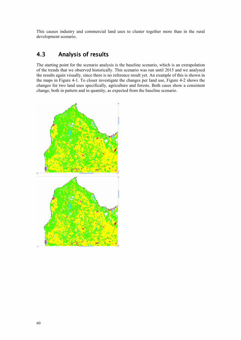
60

This causes industry and commercial land uses to cluster together more than in the rural development scenario.

4.34.34.34.3 Analysis of resultsAnalysis of resultsAnalysis of resultsAnalysis of results

The starting point for the scenario analysis is the baseline scenario, which is an extrapolation of the trends that we observed historically. This scenario was run until 2015 and we analysed the results again visually, since there is no reference result yet. An example of this is shown in the maps in Figure 4-1. To closer investigate the changes per land use, Figure 4-2 shows the changes for two land uses specifically, agriculture and forests. Both cases show a consistent change, both in pattern and in quantity, as expected from the baseline scenario.

61

Figure 4-1 Land use maps for western Latvia for 1990, 2000, and 2015 (top to bottom). Close investigation shows a consistent decrease in forested areas, that is partly taken over by new agricultural areas.

Figure 4-2: Maps indicating the difference per land use between 1990 and 2000 (top) and between 2000 and 2015 (bottom).The left two maps show the change in agricultural land and the maps on the right hand side show the difference in forested areas. For all maps, grey indicate that the land use is present in both points in time, green locations are those where the specific land use appeared over time, while red depicts the disappearance of the subsequent land uses.

The next step is the divergence into two different scenarios, the rural development and the metropolitan development scenario. Comparison of the two scenarios clearly shows a difference between the amount as well as the allocation of land use changes. This difference in allocation includes both the allocation of natural and agricultural areas as well as that of

62

urban land uses. Moreover, the differences become clear at two levels. At first the regional demands for land use classes are substantially different in the two scenarios, also the land use patterns that is generated from these demands show different characteristics.

Generally speaking, the rural development scenario shows a much more disperse development. On the one hand this means that regions that are less central and further from the large urbanized areas are developing stronger, and at the other hand it means that the new developments within this region are less clustered, and rather focussed on small cities. This development pattern is best visible in the allocation of urban land uses, such as residential land use and industrial land use. But the allocation of these land uses largely influences the agricultural and natural land uses as well.

Figure 4-3 below shows a cut-out of the generated land use maps in the south-western part of France. The left hand shows the rural development scenario, while the right hand side shows results for the metropolitan development scenario. The maps clearly show that the allocation of new industrial land use is scattered over the region in the rural development scenario and clustered around Bordeaux in the Metropolitan scenario. Figure 4-4 shows the allocation for new land uses for to types specifically: commercial and industry and forests. This figure shows more clearly the difference in amount as well as allocation of both the urban and natural land uses.

Figure 4-3 Land use maps for 2000 (top) and 2030 (bottom). The maps on the left show the results for the rural development scenario, maps on the right for the metropolitan scenario.

63

Figure 4-4 New commercial and Industrial land use (top) and forested areas (bottom) for the two scenarios. Maps on the left show the results for the rural development scenario and on the right for the Metropolitan area. Green cells depict those locations where the respective land uses appeared between 2000 and 2030.

4.3.1 Analysis of the land use patterns

The advantage of objective measures over human interpretation is obviously the ability to quantify results, which is helpful in the analysis of the land use patterns that are generated in the two scenarios. The cluster size frequency graphs show that indeed the type of differences that were anticipated in advance.

The rural development scenario shows an increase in the number of smaller clusters which is visible at the left side of the graphs. Of course this comes at the cost of the larger urban areas, which are not growing that much. The development in the Metropolitan scenario is exactly opposite; since it clearly shows that the largest clusters are growing more than in the other scenarios. This is visible form the rightmost point in the graphs shown below.

64

0

0.5

1

1.5

2

2.5

3

3.5

4

4.5

0 0.5 1 1.5 2 2.5 3 3.5

Log (size)

Lo

g (f

req

uen

cy)

Residential_2015_Baseline Residential_2015_Metropolitan Growth

Residential_2015_Rural Development

Figure 4-5 Cluster size and frequency distribution for 2015 residential land use in Western Europe

0

0.5

1

1.5

2

2.5

3

3.5

4

4.5

0 0.5 1 1.5 2 2.5 3 3.5

Log (size)

Lo

g (f

req

uen

cy)

Residential_2030_Metropolitan Growth Residential_2030_Rural Development

Figure 4-6 Cluster size and frequency distribution for 2030 residential land use in Western Europe

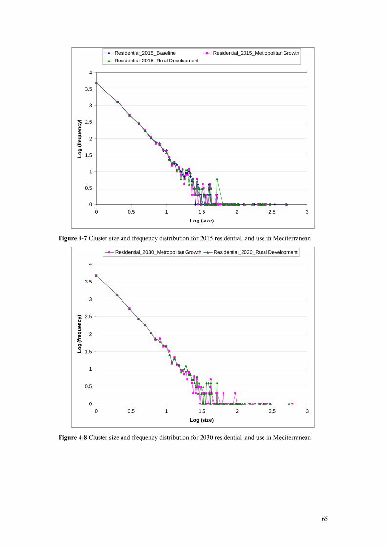
65

0

0.5

1

1.5

2

2.5

3

3.5

4

0 0.5 1 1.5 2 2.5 3

Log (size)

Lo

g (f

req

uen

cy)



Figure 4-7 Cluster size and frequency distribution for 2015 residential land use in Mediterranean

0

0.5

1

1.5

2

2.5

3

3.5

4

0 0.5 1 1.5 2 2.5 3

Log (size)

Lo

g (f

req

uen

cy)


Figure 4-8 Cluster size and frequency distribution for 2030 residential land use in Mediterranean

66

0

0.5

1

1.5

2

2.5

3

3.5

4

0 0.5 1 1.5 2 2.5

Log (size)

Lo

g (f

req

uen

cy)



Figure 4-9 Cluster size and frequency distribution for 2015 residential land use in South-eastern Europe

0

0.5

1

1.5

2

2.5

3

3.5

4

0 0.5 1 1.5 2 2.5

Log (size)

Lo

g (f

req

uen

cy)


Figure 4-10 Cluster size and frequency distribution for 2030 residential land use in South-eastern Europe

67

0

0.5

1

1.5

2

2.5

3

3.5

4

0 0.5 1 1.5 2 2.5 3

Log (size)

Lo

g (f

req

uen

cy)



Figure 4-11 Cluster size and frequency distribution for 2015 residential land use in Baltic States and North-eastern Europe

0

0.5

1

1.5

2

2.5

3

3.5

4

0 0.5 1 1.5 2 2.5 3

Log (size)

Lo

g (f

req

uen

cy)


Figure 4-12 Cluster size and frequency distribution for 2030 residential land use in Baltic States and North-eastern Europe

68

0

0.5

1

1.5

2

2.5

3

3.5

0 0.5 1 1.5 2 2.5 3

Log (size)

Lo

g (f

req

uen

cy)



Figure 4-13 Cluster size and frequency distribution for 2015 residential land use in Scandinavia

0

0.5

1

1.5

2

2.5

3

3.5

0 0.5 1 1.5 2 2.5 3

Log (size)

Lo

g (f

req

uen

cy)


Figure 4-14 Cluster size and frequency distribution for 2030 residential land use in Scandinavia

69

4.44.44.44.4 ConclusionConclusionConclusionConclusion of the scenario study of the scenario study of the scenario study of the scenario study

Three scenarios were used to create maps that show possible future land use. First there is the baseline scenario that is an extrapolation of current trends until 2015. Derived from that, two scenarios were used to create possible future land use maps for 2030. These are the rural development scenario and the Metropolitan scenario.

From the analysis of the land use maps we can say that the land use patterns that are generated are reasonable and realistic, for both scenarios. They show on a macro scale the type of patterns as well as differences that were anticipated in advance. However, a closer look at some specific regions raises the question if NUTS 2 regions are the appropriate scale for extrapolation of land use trends, since sometimes trends in neighbouring regions are opposite to an extend which is reasonable over small time scales but not when continued in an extrapolation.

Moreover some NUTS2 regions have little space left to make deviations from the baseline scenario. Specifically, the rural scenario predicts an increase in agricultural land, which was not feasible in every region for the lack of space. This required manual adjustment of the land use demands. As said, the land use that was generated eventually was realistic, but it required assumptions to come to that result.

71

ReferencesReferencesReferencesReferences

Congalton, R. (1991) A review of assessing the accuracy of classifications of remotely sensed data. Remote sensing of Environment 37: 35 – 46.

Couclelis H., Cellular Worlds: A Framework for Modelling Micro-Macro Dynamics, Environment and Planning A, 17, 585-596, 1985.

Engelen G., R. White, I. Uljee, and P. Drazan, Using Cellular Automata for Integrated Modelling of Socio-environmental Systems, Environmental Monitoring and Assessment, 30, 203-214, 1995.

Hagen, A. (2002) Multi-method assessment of map similarity. Proceedings of the 5th AGILE conference on Geographic Information Science, Palma de Mallorca, Spain.

Hagen-Zanker, A., and Lajoie, G. (2008) Neutral models of landscape change applied for the multi-scale and multi-criteria assessment of model performance. Landscape and Urban Planning 86 (3-4): 284 – 296.

McGarigal, K., Cushman, S.A., Neel, M.C. and Ene, E. (2002) FRAGSTATS: spatial analysis program for categorical maps. Computer software program produced by the authors at the university of Massachusets, Amherst. Available at www.umass.edu/landeco/research/fragstats/fragstats.html

RIKS (2005). The METRONAMICA modelling framework: model descriptions. Model documentation, Maastricht, The Netherlands.

Verburg, P.H, de Nijs. T.C.M., van Ritsema Eck, J., Visser, H., de Jong, K. (2004). A method to analyse neighborhood characteristics of land use patterns. Computers Environment and Urban System, Vol. 28(6), pp. 667–690.

White, R. and G. Engelen, Cellular Automata as the Basis of Integrated Dynamic Regional Modelling, Environment and Planning B, 24, 235-246, 1997.

White R. and G. Engelen, Cellular Automata and Fractal Urban Form: A Cellular Modelling Approach to the Evolution of Urban Land Use Patterns, Environment and Planning A, 25, 1175-1199, 1993.

White, R., The simulation of Central Place Dynamics: Two Sector Systems and the Rank-Size Distribution, Geographical Analysis, 10, 201-208, 1978.

White R., Dynamic Central Place Theory: Results of a Simulation Approach, Geographical Analysis, 9, 227-243, 1977.

White, R. (2006) Pattern based map comparisons. Journal of geographic systems 8: 145 – 164.

73

Appendix A:Appendix A:Appendix A:Appendix A: NUTSNUTSNUTSNUTS----2 regions2 regions2 regions2 regions

Table 4-4 List of NUTS-2 regions with accompanying geopolitical entity and ID number

ID NUTS2 Geopolitical

entity ID NUTS2 Geopolitical entity ID NUTS2

Geopolitical

entity

1 AT11 Burgenland 90 ES51 Cataluña 179 NL33 Zuid-Holland

2 AT12 Niederösterreich 91 ES52 Comunidad Valenciana 180 NL34 Zeeland

3 AT13 Wien 92 ES53 Illes Balears 181 NL41 Noord-Brabant

4 AT21 Kärnten 93 ES61 Andalucia 182 NL42 Limburg (NL)

5 AT22 Steiermark 94 ES62 Región de Murcia 183 PL11 Lódzkie

6 AT31 Oberösterreich 95 ES63 Ciudad Autónoma de Ceuta (ES)

184 PL12 Mazowieckie

7 AT32 Salzburg 96 ES64 Ciudad Autónoma de Melilla (ES)

185 PL21 Malopolskie

8 AT33 Tirol 97 FI13 Itä-Suomi 186 PL22 Slaskie

9 AT34 Vorarlberg 98 FI18 Etelä-Suomi 187 PL31 Lubelskie

10 BE10

Région de Bruxelles-Capitale/Brussels Hoofdstedelijk Gewest

99 FI19 Länsi-Suomi 188 PL32 Podkarpackie

11 BE21 Prov. Antwerpen 100 FI1A Pohjois-Suomi 189 PL33 Swietokrzyskie

12 BE22 Prov. Limburg (B)

101 FI20 Åland 190 PL34 Podlaskie

13 BE23 Prov. Oost-Vlaanderen

102 FR10 Île de France 191 PL41 Wielkopolskie

14 BE24 Prov. Vlaams Brabant

103 FR21 Champagne-Ardenne 192 PL42 Zachodniopomorskie

15 BE25 Prov. West-Vlaanderen

104 FR22 Picardie 193 PL43 Lubuskie

16 BE31 Prov. Brabant Wallon

105 FR23 Haute-Normandie 194 PL51 Dolnoslaskie

17 BE32 Prov. Hainaut 106 FR24 Centre 195 PL52 Opolskie

18 BE33 Prov. Liège 107 FR25 Basse-Normandie 196 PL61 Kujawsko-Pomorskie

19 BE34 Prov. Luxembourg (B)

108 FR26 Bourgogne 197 PL62 Warminsko-Mazurskie

20 BE35 Prov. Namur 109 FR30 Nord - Pas-de-Calais 198 PL63 Pomorskie

21 BG11 Severozapaden 110 FR41 Lorraine 199 PT11 Norte

22 BG12 Severen tsentralen

111 FR42 Alsace 200 PT15 Algarve

23 BG13 Severoiztochen 112 FR43 Franche-Comté 201 PT16 Centro (PT)

24 BG21 Yugoiztochen 113 FR51 Pays de la Loire 202 PT17 Lisboa

25 BG22 Yuzhen tsentralen

114 FR52 Bretagne 203 PT18 Alentejo

26 BG23 Yugozapaden 115 FR53 Poitou-Charentes 204 RO01 Nord-Est

27 CY00 Cyprus 116 FR61 Aquitaine 205 RO02 Sud-Est

28 CZ01 Praha 117 FR62 Midi-Pyrénées 206 RO03 Sud - Muntenia

29 CZ02 Strední Cechy 118 FR63 Limousin 207 RO04 Sud-Vest Oltenia

30 CZ03 Jihozápad 119 FR71 Rhône-Alpes 208 RO05 Vest

31 CZ04 Severozápad 120 FR72 Auvergne 209 RO06 Nord-Vest

32 CZ05 Severovýchod 121 FR81 Languedoc-Roussillon 210 RO07 Centru

74



Geopolitical

entity

33 CZ06 Jihovýchod 122 FR82 Provence-Alpes-Côte d'Azur 211 RO08 Bucuresti - Ilfov

34 CZ07 Strední Morava 123 FR83 Corse 212 SE01 Stockholm

35 CZ08 Moravskoslezsko 124 GR11 Anatoliki Makedonia, Thraki 213 SE02 Östra Mellansverige

36 DE11 Stuttgart 125 GR12 Kentriki Makedonia 214 SE04 Sydsverige

37 DE12 Karlsruhe 126 GR13 Dytiki Makedonia 215 SE06 Norra Mellansverige

38 DE13 Freiburg 127 GR14 Thessalia 216 SE07 Mellersta Norrland

39 DE14 Tübingen 128 GR21 Ipeiros 217 SE08 Övre Norrland

40 DE21 Oberbayern 129 GR22 Ionia Nisia 218 SE09 Småland med öarna

41 DE22 Niederbayern 130 GR23 Dytiki Ellada 219 SE0A Västsverige

42 DE23 Oberpfalz 131 GR24 Sterea Ellada 220 SI00 Slovenia

43 DE24 Oberfranken 132 GR25 Peloponnisos 221 SK01 Bratislavský kraj

44 DE25 Mittelfranken 133 GR30 Attiki 222 SK02 Západné Slovensko

45 DE26 Unterfranken 134 GR41 Voreio Aigaio 223 SK03 Stredné Slovensko

46 DE27 Schwaben 135 GR42 Notio Aigaio 224 SK04 Východné Slovensko

47 DE30 Berlin 136 GR43 Kriti 225 UKC1 Tees Valley and Durham

48 DE41 Brandenburg - Nordost

137 HU10 Közép-Magyarország 226 UKC2 Northumberland, Tyne and Wear

49 DE42 Brandenburg - Südwest

138 HU21 Közép-Dunántúl 227 UKD1 Cumbria

50 DE50 Bremen 139 HU22 Nyugat-Dunántúl 228 UKD2 Cheshire

51 DE60 Hamburg 140 HU23 Dél-Dunántúl 229 UKD3 Greater Manchester

52 DE71 Darmstadt 141 HU31 Észak-Magyarország 230 UKD4 Lancashire

53 DE72 Gießen 142 HU32 Észak-Alföld 231 UKD5 Merseyside

54 DE73 Kassel 143 HU33 Dél-Alföld 232 UKE1 East Riding and North Lincolnshire

55 DE80 Mecklenburg-Vorpommern

144 IE01 Border, Midlands and Western 233 UKE2 North Yorkshire

56 DE91 Braunschweig 145 IE02 Southern and Eastern 234 UKE3 South Yorkshire

57 DE92 Hannover 146 ITC1 Piemonte 235 UKE4 West Yorkshire

58 DE93 Lüneburg 147 ITC2 Valle d'Aosta/Vallée d'Aoste 236 UKF1 Derbyshire and Nottinghamshire

59 DE94 Weser-Ems 148 ITC3 Liguria 237 UKF2 Leicestershire, Rutland and Northants

60 DEA1 Düsseldorf 149 ITC4 Lombardia 238 UKF3 Lincolnshire

61 DEA2 Köln 150 ITD1 Provincia Autonoma Bolzano-Bozen

239 UKG1 Herefordshire, Worcestershire and Warks

62 DEA3 Münster 151 ITD2 Provincia Autonoma Trento 240 UKG2 Shropshire and Staffordshire

63 DEA4 Detmold 152 ITD3 Veneto 241 UKG3 West Midlands

64 DEA5 Arnsberg 153 ITD4 Friuli-Venezia Giulia 242 UKH1 East Anglia

65 DEB1 Koblenz 154 ITD5 Emilia-Romagna 243 UKH2 Bedfordshire, Hertfordshire

66 DEB2 Trier 155 ITE1 Toscana 244 UKH3 Essex

67 DEB3 Rheinhessen-Pfalz

156 ITE2 Umbria 245 UKI1 Inner London

68 DEC0 Saarland 157 ITE3 Marche 246 UKI2 Outer London

69 DED1 Chemnitz 158 ITE4 Lazio 247 UKJ1 Berkshire, Bucks and Oxfordshire

70 DED2 Dresden 159 ITF1 Abruzzo 248 UKJ2 Surrey, East and West Sussex

71 DED3 Leipzig 160 ITF2 Molise 249 UKJ3 Hampshire and Isle of Wight

72 DEE1 Dessau 161 ITF3 Campania 250 UKJ4 Kent

73 DEE2 Halle 162 ITF4 Puglia 251 UKK1 Gloucestershire, Wiltshire and North Somerset

74 DEE3 Magdeburg 163 ITF5 Basilicata 252 UKK2 Dorset and Somerset

75



Geopolitical

entity

75 DEF0 Schleswig-Holstein

164 ITF6 Calabria 253 UKK3 Cornwall and Isles of Scilly

76 DEG0 Thüringen 165 ITG1 Sicilia 254 UKK4 Devon

77 DK00 Denmark 166 ITG2 Sardegna 255 UKL1 West Wales and The Valleys

78 EE00 Estonia 167 LT00 Lithuania 256 UKL2 East Wales

79 ES11 Galicia 168 LU00 Luxembourg (Grand-Duché) 257 UKM1 North Eastern Scotland

80 ES12 Principado de Asturias

169 LV00 Latvia 258 UKM2 Eastern Scotland

81 ES13 Cantabria 170 MT00 Malta 259 UKM3 South Western Scotland

82 ES21 Pais Vasco 171 NL11 Groningen 260 UKM4 Highlands and Islands

83 ES22 Comunidad Foral de Navarra

172 NL12 Friesland 261 UKN0 Northern Ireland

84 ES23 La Rioja 173 NL13 Drenthe

85 ES24 Aragón 174 NL21 Overijssel

86 ES30 Comunidad de Madrid

175 NL22 Gelderland

87 ES41 Castilla y León 176 NL23 Flevoland

88 ES42 Castilla-la Mancha

177 NL31 Utrecht

89 ES43 Extremadura 178 NL32 Noord-Holland

assessment and scenarios aassessment and scenar … · aaassessment and scenarios ssessment and...

Documents