assessment of soil organic carbon stocks in the … · comunidades no interior do parque e cuja...
TRANSCRIPT

ASSESSMENT OF SOIL ORGANIC CARBON STOCKS IN THE LIMPOPO NATIONAL PARK: FROM LEGACY DATA TO DIGITAL SOIL MAPPING
Armindo Henrique Cambule

Examining committee: Prof.dr.ir. A. Veldkamp University of Twente Prof.dr.ir. A. Stein University of Twente Prof.dr. E. Hoffland Wageningen University and Research Centre Prof.dr. F.D. van der Meer University of Twente ITC dissertation number 227 ITC, P.O. Box 217, 7500 AA Enschede, The Netherlands ISBN 978-90-6164-355-5 Cover designed by Benno Masselink Printed by ITC Printing Department Copyright © 2013 by Armindo Henrique Cambule

ASSESSMENT OF SOIL ORGANIC CARBON STOCKS IN THE LIMPOPO NATIONAL PARK: FROM LEGACY DATA TO DIGITAL SOIL MAPPING
DISSERTATION
to obtain the degree of doctor at the University of Twente,
on the authority of the rector magnificus, prof.dr. H. Brinksma,
on account of the decision of the graduation committee, to be publicly defended
on Friday 21 June 2013 at 14.45 hrs
by
Armindo Henrique Cambule
born on 5 June 1967
in Inhambane, Mozambique

This thesis is approved by Prof.dr.ir. E.M.A. Smaling, promoter Dr. D.G. Rossiter, assistant promoter Dr.ir. J.J. Stoorvogel, assistant promoter

Abstract In 2001, Mozambique declared an area known as “Coutada 16” (hunting zone) the Limpopo National Park (LNP), which forms part of a trans-frontier park with South Africa and Zimbabwe. The park provides ecosystem services and supports the livelihoods of thousands people living in the many communities within its boundaries, which were planned for relocation outside the park. These moves were expected to result in major land use changes, both in terms of vegetation and wildlife, affecting soil quality in and around the LNP, including in resettlement areas. Therefore, this study aimed at estimating soil organic carbon (SOC) stocks in the Limpopo National park as an indicator of livelihoods and ecosystem function. The estimation of SOC stocks was first attempted from legacy data then by both measure-and-multiply and digital soil mapping (DSM) based on a new sampling plan. Along this study issues of legacy data renewal quality, mapping data-poor and poorly-accessible areas, time-consuming and costly traditional method for SOC laboratory determination as well as uncertainty and reliability of SOC stocks estimates from different methods were also investigated. Overall this research provided (1) a guiding framework and quantitative measures for evaluation of renewed legacy survey and as such enabled an informed qualitative and quantitative SOC stocks estimation, (2) a cost-effective methodology for mapping SOC in data-poor, poorly-accessible areas following a DSM approach, (3) a rapid, cost-effect, non-destructive and pollutant-free Near-Infrared a calibration model for the determination of SOC in LNP and, (4) SOC stocks estimates, its uncertainty and reliability. Despite the high uncertainty of the estimates, which limit its use in baseline studies, achieved SOC stocks estimates are, in general, consistent with of SOC stocks estimates in the literature for similar soils in comparable environmental conditions in southern Africa.

Resumo Em 2001, Mozambique declarou a área conhecida como “Coutada 16” (zona de caca) de Parque Nacional do Limpopo (PNL), que compõe o parque transfronteiriço com a Africa do sul e o Zimbabwe. O parque fornece serviços e suporta “o sustento/livelihood” de milhares de pessoas vivendo em muitas comunidades no interior do parque e cuja realocação foi planificada para o exterior do parque. Espera-se que estas acções resultem em grandes mudanças do uso de terra em termos de vegetação e vida selvagem e que afectarão a qualidade do solo dentro e cercanias do PNL. Por isso, o presente estudo visa estimar o “stock” de carbono orgânico do solo (COS) do parque como indicador do “livelihood” e “função” do ecossistema. A estimativa do COS foi inicialmente feita com recurso ao legado-de-dados e posteriormente com base no método “measure-and-multiply” e mapeamento digital do solo (MDS), ambos com recurso a uma nova amostragem de campo. Ao longo do estudo, questões da qualidade de legado-de-dados renovados, mapeamento de áreas pobres em dados e com pouco acessíveis, os dispendiosos e lentos métodos tradicionais de análises laboratoriais para a determinação do COS bem como “incertezas” e “confiança” das estimativas de COS pelos diferentes métodos foram investigadas. Da pesquisa resultou (1) um quadro-guia e medidas quantitativas para a avaliação de inventários-legado e como tal permitiu estimativa qualitativa e quantitativa da estimativa do “stocks” de COS, (2) uma metodologia custo-efectiva para o mapeamento de COS em áreas pobres de dados e de limitado acesso pelo “approach” MDS, (3) um modelo de calibração NIR para a determinação do COS para o PNL; rápido, custo-efectivo, não-destrutivo e livre de poluentes e, (4) estimativas de “stocks” de COS, suas “incertezas/uncertainty” e grau de confiança. Não obstante a elevada “incerteza/uncertainty” das estimativas do COS que limitam o seu uso em estudos de base, as mesmas são em geral consistentes com valores na literatura referentes a solos similares em condições em ambientais também comparáveis, na região austral de Africa.
ii

Acknowledgements It all started in mid-October when Ken Giller invited me to study the role of spatial of SOC as an indicator of sustainability and livelihood in southern Africa, project nr 12, within the scope of the Competing claims on natural resources programme (CCNR, www.competingclaims.nl). We had met for the first time few weeks earlier in Blantyre, Malawi while attending the joint TF planning workshop of the FARA SSA-challenge programme. Maja Slingerland and Marc van den Vijver followed up the initiate and helped with all paperwork to join the CCNR programme and be able to attend the CCNR kick-off workshop held at the Wageningen University. It was at this workshop where I met the supervisory team; Professors Eric Smaling, Jetse J. Stoorvogel and David G. Rossiter with whom I planned the all research, from scoping study to research project proposal. Loes Colenbrander helped with paperwork to join ITC. The establishment of the LNP was expected to result in major land use changes which would impact on thousands people living in the many communities within its boundaries, which were planned for relocation outside the park, which provides ecosystem services and supports the livelihoods. This formed the starting point of the research, summarized in this book which reports the result of the research on the estimation of soil organic carbon (SOC) stocks and its spatial distribution in the LNP. SOC as a proxy indicator of land use changes. The research provided insights into SOC estimation from NIR-spectroscopy, the quality aspects in re-using legacy data for SOC stocks estimation, the role of DSM for SOC stocks in mapping data-limited and poorly-accessible areas. The successful completion this work was possible thanks to the help from so many people. Ken Giller, Maja Slingerland, Marc van de Vijver and Loes Colenbrander for reasons mentioned above. Eric Smaling, Jetse Stoorvogel and David Rossiter for the teamwork and supervision. Jens Anderson and Almeida Sitoe (CCNR regional and national coordinator) for local supervision. Thank you for the support. I extend my sincere thanks to the soil section team a ICRAF, Nairobi for providing the training in NIR-spectroscopy. To Professor Russel Yost for helping in the setting and calibration of NIR spectrometer and also for support while at Faculty of Agronomy on his Sabbaticals. To the IIAM team, M Vilanculos, R Maria, Sitoe, O Jalane and J Francisco. Thank you all.
iii

I had the chance to meet many CCNR fellows and friends with whom I had long discussions on various PhD topics, in and outside the formal discussion groups, annual meetings. Dr Abel Ramoelo, Dr Petronnela Chaminuka, Dr Chrispan Murunguene, Xavier Poshiwa, Dr Jessica Milgroom, Nicia Giva and many more. Thank you all for being there for me. At ITC I had the privilege of meeting fellow PhD students from around the world with whom I interacted almost on a daily basis; my office mates Diviyani, Debanjan, Rafael, Dr Khan, Emmanual, …. and other fellows, Dr Ha, Mariela, Adrie, Dr Fekerte, Dr Mariela, Adri , Dr Si Yali, Maitreyi, Priya, Anandita, Sabrina, Dr Tagel, Dawit, Atkilt, Vincent, Francis, John, Nthabi, Sibu and many others. Thank you all. I was granted permission to carry out the fieldwork by the Ministry of Tourism so would like to thank all the officials from both the Ministry and the LNP for making the “tour” as smooth as possible. The unforgettable fieldwork in the LNP was possible thanks to the help from my colleague R Borguete and the LNP ranger Lourenco (txacuatica) who made sure of our safety 24/7. The three of us shaped a perfect team as we sampled, run away from Elephants, lions, Mambas, etc. I stepped on a snear and you guys managed to safely pull me out of it, thank you so much. The Mozambican community and friends in the Netherlands made my stay in The Netherlands more enjoyable. The Mabyaias (Messias, Liza), Joaninha. Maurits van den Berg, Hans Kok & Liza, thank you for the hospitality. While away my colleagues and faculty members had the burden of replacing me in teaching and all other academic activities, Engos. Massingue, Borguete, Lumbela, Dr Famba and Dr Alfredo Nhantumbo, Romano Guiamba, Albano Tomo, Antonio Machava, E. Macamo. My sincere thanks. Last but not least to my wife (Marcela), children (Mauro, Eniciah, Michelle), Brothers and sisters (Adelaide, Kinho, Marta, Rosta, Nricky) and entire family, Thank you for the support and brotherhood. Mom & Dad: here is the book, thank you for the tireless support and comfort.
iv

Table of Contents Abstract i Resumo ii Acknowledgements ............................................................................... iii Chapter 1 Soil organic carbon as a proxy indicator of soil quality and
sustainability in LNP ................................................................. 1 1.1 Introduction ............................................................................ 2 1.2 Soil organic carbon: legacy data quality, estimation from NIR
spectroscopy and spatial prediction ............................................ 4 1.3 Research aim and objectives ..................................................... 6 1.4 Outline of the thesis ................................................................. 6 1.5 The research site ..................................................................... 8
Chapter 2 Legacy soil data rescue and renewal – a case study of the LNP . 13 2.1 Introduction .......................................................................... 15 2.2 Material and methods ............................................................. 17
2.2.1 Geodetic control ............................................................. 18 2.2.2 Creation of GIS layers ..................................................... 18 2.2.3 Integration of remotely-sensed data and digital elevation
model ........................................................................... 19 2.2.4 Metadata ....................................................................... 20 2.2.5 Spatial data infrastructure ............................................... 21 2.2.6 Inference about SOC stocks ............................................. 21
2.3 Results and discussion ............................................................ 21 2.3.1 Legacy data archeology and a brief history of soil resource
inventory in the LNP........................................................ 21 2.3.2 Selection of legacy soil surveys vicinity ............................. 23 2.2.3 Renewal of Legacy survey ................................................ 26
2.4 Summary and Conclusion........................................................ 42 Chapter 3 A DSM methodology for poorly accessible area ........................ 45
3.1 Introduction .......................................................................... 47 3.2 Material and methods ............................................................. 48 3.3 Results and discussion ............................................................ 56
3.3.1 Explanatory variables ...................................................... 56 3.3.2 Strata based on accessibility, similarity analysis ................. 58 3.3.3 Primary data collection and laboratory analysis .................. 61 3.3.4 Development of the spatial prediction model ...................... 62 3.3.5 Application of the model in accessible area ........................ 68 3.3.6 Model validation in accessible areas .................................. 70 3.3.7 Application of the model in poorly-accessible areas ............. 71 3.3.8 Model validation in poorly-accessible areas ........................ 72 3.3.9 Relative performance of prediction model in PACC areas ...... 72
3.4 Conclusions ........................................................................... 73 Chapter 4 Building a NIR spectral library for the LNP .............................. 75
4.1 Introduction .......................................................................... 77 4.2 Materials and methods ........................................................... 78
v

4.2.1 Soil samples and spectral acquisition ................................ 78 4.2.2 Selection of soil samples for reference analysis .................. 79 4.2.3 Laboratory analysis ......................................................... 79 4.2.4 Calibration and validation ................................................ 80
4.3 Results and discussion ............................................................ 81 4.3.1 Sample selection for reference analysis ............................. 81 4.3.2 Soil properties ................................................................ 81 4.3.3 Laboratory SOC vs Landscape units .................................. 83 4.3.4 Spectral features ............................................................ 84 4.3.5 Prediction of SOC from NIR spectra ................................... 85 4.3.6 Calibration subset models ................................................ 90 4.3.7 Prediction of SOC from NIR spectra and Clay ...................... 90
4.4 Conclusions ........................................................................... 90 Chapter 5 SOC stocks in the LNP - Amount, spatial distribution and
uncertainty ........................................................................ 93 5.1 Introduction .......................................................................... 95 5.2 Material and methods ............................................................. 96
5.2.1 Assessing SOC stocks ...................................................... 97 5.3 Results and discussion ........................................................... 100
5.3.1 SOC stocks at sampling points ........................................ 100 5.3.2 Assessing SOC stocks spatial distribution .......................... 103 5.3.3 Total SOC stocks estimates and their uncertainty .............. 112 5.3.4 Reliability of SOC stocks estimates and potential
improvements ............................................................... 113 5.4 Conclusions .......................................................................... 116
Chapter 6 Synthesis and Conclusions ................................................... 119 6.1 Synthesis and discussion ....................................................... 120
6.1.1 Renewing legacy soil data for SOC stocks estimation: is it worth the trouble? ......................................................... 120
6.1.2 Mapping SOC in poorly-accessible areas ........................... 120 6.1.3 Near-infrared spectroscopy: a rapid, non-destructive and
environmentally friendly lab method ................................ 122 6.1.4 SOC stocks in LNP; amount, spatial distribution and uncertainty ................................................................... 124
6.2 Concluding remarks .............................................................. 125 6.3 Recommendations................................................................. 126
6.3.1 Application of the results of this study .............................. 126 6.3.2 Recommendations for further research ............................. 127
References ........................................................................................ 129 Summary .......................................................................................... 141 Samenvatting .................................................................................... 145 Author’s Biography ............................................................................. 149 ITC Dissertation List ........................................................................... 151
vi

Chapter 1 Soil organic carbon as a proxy indicator of soil quality and sustainability in LNP
1

Soil organic carbon as a proxy indicator of soil quality and sustainability in LNP
1.1 Introduction In 2001, Mozambique declared an area known as “Coutada 16” (hunting zone) the Limpopo National Park (LNP), which forms part of a trans-frontier park with South Africa and Zimbabwe. The LNP provides ecosystem services and supports the livelihoods of about 20 000 people living within its boundaries. The formation of LNP and the planned relocation of the communities within the park will result in major land use changes, both in terms of vegetation and wildlife (Ministerio do Turismo, 2003). These changes are expected to affect soil quality in and around the LNP, including in resettlement areas. The demand for arable land, grazing, forestry, wildlife, tourism and community development is greater than land resources available so soil quality may worsen. Therefore, sustainable land management is needed. It aims at harmonizing the complementary goals of providing environmental, economic, and social opportunities for the benefit of present and future generations, while maintaining and enhancing the quality of land resource. This can only be achieved through interactive planning which allows monitoring how far a land use plan is meeting the goals set and change whenever felt necessary (Dumanski, 1998; FAO, 1993). Therefore, there is a need to monitor soil quality so land use management plan can be timely adjusted to achieve sustainability. The need for sustainable land management has raised an unfinished scientific discussion about the definition of soil quality and relevant indicators to quantify it. Nevertheless, many authors have used soil organic matter content (SOM) as an indicator of the impacts of land use changes, because SOM is (Batjes, 1992) probably the most important soil constituent. SOM is defined as the organic constituents of the soil, excluding undecayed plant and animal tissue, their partial decomposition products and the soil biomass. The definition, therefore, includes the identifiable high-molecular weight organic material such as polysaccharides and proteins, simpler substances such as sugars, amino acids, and other small molecules, and humic substances (Batjes, 1992). Decaying SOM releases essential nutrients for plant and microbial growth. SOM is an important determinant of cation exchange capacity, particularly in coarse-textured soils and on low activity clay soils, serves as reservoir of nutrients and water, aids in reducing compaction, surface crusting and improves structure, aeration, infiltration, permeability, aggregate stability and buffering capacity. It also protects soils against erosion. This implies that SOM content strongly influences soil productivity (Batjes, 1992). SOM content is affected by climate, soil mineralogy and fertility, soil texture,
2

Chapter 1
structure and biodiversity, vegetation and land use changes or successions (Batjes, 1992) so, the role of SOM can be diminished by these factors leading to CO2 emission (Kamoni et al., 2007; Milne et al., 2007), loss of its favourable effects (e.g. soil structure), soil erosion and overall land degradation (Gisladottir and Stocking, 2005). Climate controls biophysical production potential; the net primary production (NPP). SOM levels are regulated by the net primary production, distribution of photosynthates into roots and shoots and the rate at which these organic residues decompose (Batjes, 1992). Climate and its changes affect SOM through changes in rainfall patterns and its effect on biomass production, as the low rainfall range and few but intense rainstorms cause high erosion but are insufficient to result in good vegetation cover (Gisladottir and Stocking, 2005) whose decomposing residues lead to formation of SOM, and thus contribute to land degradation. Soil organic carbon (SOC) is the main constituent of SOM and many studies have shown its importance as a soil quality indicator both as a single soil or compound (SOM) attribute (Arshad and Martin, 2002; Brejda et al., 2000a; Brejda et al., 2000b; Yemefack et al., 2006). SOC plays an important role in terrestrial ecosystems for human well-being, which has made it a good proxy indicator of both environmental goods and services (such as crops, grass for range, but also water storage, soil biology and nutrient cycling). Of most interest is perhaps the fact that soils are the main terrestrial pool of organic carbon and therefore fixing/sequestration of carbon is the single best entry point for land degradation control through which mankind will be able to control land degradation and therefore pursue sustainable land management (Gisladottir and Stocking, 2005); the maintenance of good soil quality. The widely-used soil fertility-crop production model QUEFTS uses SOC, or total nitrogen as a proxy (assuming a stable C/N ratio), as the major yield-explaining variable (Janssen et al., 1990; Liu et al., 2006; Pathak et al., 2003; Smaling and Janssen, 1993). This comes as no surprise in strongly weathered tropical soils that largely rely on the organic fraction for their inherent soil fertility. These evidences support Shukla et al. (2006) who stated that if only one soil attribute were to be used for monitoring soil quality changes, it should be SOC. Any change in soil quality cannot be assessed without a proper baseline, i.e., present-day soil quality. As part of a project on “competing claims in natural resources” in the trans-frontier national park areas of Mozambique, RSA and Zimbabwe (Giller et al., 2008), there was a need to assess soil resources in the LNP of Mozambique, specifically the SOC stocks as an indicator of livelihoods and ecosystem function.
3

Soil organic carbon as a proxy indicator of soil quality and sustainability in LNP
This book discusses the processes through which the SOC concentration and stocks were estimated as well as the respective spatial distribution and finally the total SOC stocks for an extensive, poorly-accessible and data-poor area. As part of this process, issues of legacy data quality, laboratory determination of SOC using rapid, non-destructive technique as well as alternative mapping methodology for mapping poorly-accessible areas are discussed.
1.2 Soil organic carbon: legacy data quality, estimation from NIR spectroscopy and spatial prediction
Many developing countries are covered by legacy soil surveys, usually the only source of information because it is unlikely that new soil surveys can be commissioned. Despite the valuable information gathered at considerable effort and cost, this legacy data is in many cases hardly used. Some reasons for this lack of use are poor availability, poor documentation, and the outdated data (currency; as soil properties may have changed) and survey concepts and standards by which the maps were made, making them not adequate for decision making. Consequently these legacy surveys are likely to be ignored or even lost (Rossiter, 2008). If retrieved, legacy soil surveys can also be valuable baselines for monitoring, e.g., of changes in soil organic Carbon stocks and land degradation or rehabilitation, allowing therefore historical re-look. Legacy SRI needs first to be well documented and properly preserved in order to be re-used. A good example of this is the European Archive of Digital Soil Maps of Africa (Selvaradjou et al., 2005), where maps from many legacy maps from African countries were scanned and archived in an optical digital media. In this way the maps will be better preserved for future use. Given the currency issues of legacy soil data, the challenge is then how can we make best use of them. Two good examples of re-use of legacy data are by Dent & Ahmed (1995) and Ahmed and Dent (1997) who used statistical techniques to test and re-interpret archival data from soil survey of the tidal floodplain of the Gambia River. From their re-interpretation the authors concluded that the intuitively defined and mapped soil series from the original survey did not match the soil taxonomic units derived by cluster analysis of validated data. This insight was possible due to the added value of geostatistics for the re-use of legacy soil survey data. In recent years soil survey procedures have been revolutionized by the use of geo-information technology, including remotely-sensed imagery, digital elevation models (DEM), and statistical inference models; the emerging
4

Chapter 1
paradigm is called digital soil mapping (DSM), summarized by McBratney et al. (2003) and the subject of several international workshops (Hartemink and McBratney, 2008; Lagacherie et al., 2007) which can be applied to improve various aspects of legacy SRI (Rossiter, 2008). This author lays out a conceptual framework for using DSM techniques to support legacy data renewal with emphasis on areas with sparse soil data infrastructures, and soil maps following the discrete model of spatial variation. The author further gives an example where soil unit boundaries of a 1:50.000 Kenyan soil map are checked based on identifiable landscape features from a draped DEM on the soil map. Despite the improvement that can be made to legacy SRI data, the author did not assess the degree of improvement made. In this study the conceptual framework for using DSM techniques to support legacy data renewal by Rossiter (2008) was tested and the various criteria from the guidelines for evaluating the adequacy of soil resource inventories (Forbes et al., 1982) were applied, to assess the quality of renewed legacy soil data, and the approaches and strategies to improve legacy SRI data renewal even further were discussed. In the event that new soil surveys are commissioned, current SOC data can be obtained as part of the survey. Traditionally the knowledge of spatial distribution of soil properties is represented as soil maps conforming to the discrete model of spatial variation; DMSV (Heuvelink and Webster, 2001), showing polygons within which soils are considered homogeneous and with boundaries where changes in soil properties are considered to be abrupt. Soil properties of the different units were characterized by collecting large number of “representative” samples, subjected to traditional time-consuming and costly laboratory analysis. The recent rapid development of information technology along with the availability of new types of secondary data (e.g., digital elevation models and satellite imagery) allow for more quantitative approach (continuous model of spatial variation; CMSV) to soil survey producing surfaces based on soil forming factors. Furthermore, these methods give spatial estimates of the uncertainty of the predictions. This “predictive” (Scull et al., 2003) or “digital” soil mapping; DSM (McBratney et al., 2003) uses relationships between soil properties and auxiliary data at sample points to predict over a study area. Digital soil mapping (DSM) techniques have been successfully applied in studies at field scale where soil variability is largely due to the effect of topography on soil genesis (e.g., Florinsky et al., 2002) and therefore much of the success is attained by integration of terrain attributes as auxiliary data. The challenge is to capture the spatial structure of soil variation as well as the soil-environment relations over larger poorly-accessible areas due to poor
5

Soil organic carbon as a proxy indicator of soil quality and sustainability in LNP
road networks (such as much of Africa) or difficult terrain (e.g., mountainous regions), a large number of observations following a sound sampling design, covering the feature and geographic space of the predictors (e.g., Minasny and McBratney, 2006) are required, which is impractical or prohibitively expensive. In this book an alternative DSM approach is proposed, in which sampling is concentrated along accessible areas and samples are then used to build the DSM model, which is later applied to predict over the large poorly-accessible area. In between sampling and DSM model building, the traditional time-consuming, costly laboratory analyses that may result in environmental pollutants were replaced by applying the promising new technique in the field of diffuse reflectance spectroscopy (e.g. Near-Infrared spectroscopy, NIR), a fast, non-destructive and inexpensive soil analysis (Shepherd and Walsh, 2002; Viscarra-Rossel and McBratney, 2008). However, the technique requires building robust both spectral libraries and model to describe the relation between soil attribute and its spectral signature. The challenge is to minimize the size of spectral library needed to capture all variability, especially in areas where no spectral library exists. The SOC-NIR calibration model built on the base of a limited sub-set of collected samples was later used to estimate SOC for the entire field collected samples. Finally and following the DSM approach and results, the SOC stocks, its spatial distribution, total SOC stocks and uncertainty were estimated for the study area.
1.3 Research aim and objectives The aim of this study was to develop alternative methods to obtain SOC data in the LNP. Specific objectives were to (1) test the use of various criteria for evaluating the adequacy of soil resource inventories, to assess the quality of renewed legacy soil data, with emphasis on SOC stocks estimation (2) to develop an alternative DSM method for the prediction of SOC in a large, poorly-accessible area, (3) to test and assess the robustness of a NIR calibration model built from a limited number of samples for the estimation of SOC, and (4) to predict SOC stocks, its spatial distribution and uncertainty in the LNP.
1.4 Outline of the thesis This research carried out in this study is reported in six chapters, including the introduction and Synthesis. The analysis are based on field measured A-horizon depth, laboratory determinations of SOC concentration, particle size and acquisition NIR spectral signature of field collected soil samples collect across the study area. This book is organized to address issues related to
6
Chapter 1
SOC data for the estimation of stocks in an extensive, data-poor and poorly-accessible area. Chapter 1 This chapter introduces the research problem, aim and objectives. It also defines SOC and discusses its role in the context of soil quality. The chapter also reviews the benefits and limitations faced to make use of legacy SOC data, reviews the challenges to estimate SOC in the laboratory as well as the modeling of spatial distribution of SOC concentration and stocks. Chapter 2 The objective was to assess quality of rescued legacy soil map. Legacy soil maps from the study area were rescued and renewed following the conceptual framework for data rescue and renewal. The assessment of renewed legacy soil maps was made using the Cornell adequacy criteria for the evaluation of SRI. Rescued legacy data with good quality can be used to estimate SOC stocks. Chapter 3 This chapter had the objective of developing a cost-efficient methodology for digital soil mapping in poorly-accessible areas. In this chapter, a stepwise approach to predict the spatial distribution of SOC concentration is proposed. The spatial model is developed based on laboratory SOC data determined from limited soil samples collected across the study area, chiefly in accessible areas. Chapter 4 This chapter intercalated the previous one. The objective was to test the possibility of calibrating a useful NIR-calibration model for the prediction of SOC concentration based on a limited number of soil samples. The limited number of samples was assumed to reflect the “poor accessibility” problem of the study area due to limited road network, wildlife hazard and rough terrain. The analysis was performed on a sub-set of soil samples from previous chapter. Calibrated model was then used to estimate SOC in remainder of soil sample, later used to develop spatial model for the spatial prediction of SOC (previous chapter). Chapter 5 This chapter had the objective of assessing the total SOC stock, its spatial variation and the causes of such variation the study area. The analysis included the calibration of spatial model which made use of a limited number (typical of poorly accessible areas) of field measures A-horizon depth and SOC data predicted using the NIR-calibration model (chapter 4). The spatial
7

Soil organic carbon as a proxy indicator of soil quality and sustainability in LNP
model made also use of secondary data to represent the soil forming factor’s explanatory variables. Chapter 6 This chapter synthesizes the major issues derived from this study, specifically in obtaining SOC data from legacy sources, laboratory measurements and predicting SOC concentration and stocks. Focus is given for data-poor and poorly-accessible areas, typical of most developing countries. This chapter also provides recommendations for application of results from this study and for future research of question not solved in this study.
1.5 The research site The LNP was selected as the study area. It is located in the western part of Gaza province (south of Mozambique) and is one part of the study area of the “Competing Claims on Natural Resources” programme (Giller et al., 2008), centered on the trans-frontier national parks of the Mozambique-Zimbabwe-South Africa border (Figure 1.1). LNP is located in Mozambique between 22° 25' and 24° 10' S and 31° 18' and 32° 38' E and is delimited by about 190 Km fenced international border with South Africa (Kruger National Park) to the west, and by both Limpopo (about 260 Km) and Elephant (about 85 Km) Rivers, east and south, respectively, covering a total of about 10 500 km2. Altitudes range from about 50 to about 500 m above sea level (Stalmans et al., 2004). It has a warm arid climate (BWh, Köppen classification) with a dry winter and mean annual temperature exceeding 18° C (Peel et al., 2007). Absolute maximum temperatures (between November and February) increase northwards to above 40°C. Annual rainfall decreases northwards from above 500 mm in the southeast to about 350 mm at the extreme north (Ministerio do Turismo, 2003; Stalmans et al., 2004).
8

Chapter 1
Figure 1.1: The Great Limpopo Trans-frontier Park (left) formed by the Gonareshu National Park (GNP), the Kruger National Park (KNP) and the study area of this research; the Limpopo National Park (LNP), within which the detail of legacy data renewal study area (right) in shown around Massingir. The dominant lithology is the extensive Quaternary aeolian sand cover along the NNW-SSE spine of the park. Tertiary sedimentary rocks (limestones, sandstone) are found close to the drainage lines where the sand mantle has been exposed. Rhyolite rocks from the Karroo formation are located along the western border while alluvium lies along the main drainage lines. Soils derived from aeolian sands range from shallow to deep and are sandy, those derived from rhyolite are shallow and clayey, those derived from sedimentary rocks are deep, structured and clayey and those derived from alluvium materials are clayey (Manninen et al., 2008; Rutten et al., 2008; Stalmans et al., 2004).
9

Soil organic carbon as a proxy indicator of soil quality and sustainability in LNP
Figure 1.2: The SRTM digital elevation model and annual precipitation (Hijmans et al., 2011) distribution across the LNP. The LNP is poorly covered by systematic soil survey. Instead, a few detailed soil surveys around the Massingir dam reservoir were carried out for irrigation planning in the late colonial and early post-colonial times. The national reconnaissance soil map at 1:1.000.000 scale shows the LNP covered by five soil units from five major soil groups (FAO and Unesco, 1997; INGC et al., 2003; INIA, 1995); the Arenosols/Haplic Luvisols and Ferralic Arenosols on the Quaternary aeolian sands, the Eutric Leptosols over the Karroo formation, and the Calcaric Cambisols and Eutric Fluvisols along the main drainage lines. Stalmans et al. (2004) classified LNP into ten major landscape units (1) Combretum spp./ Colophospermum mopane Rugged Veld (CMR), characterised by shallow soils on the hills but deeper in the footslopes and low-lying areas, (2) Limpopo Levubu Floodplains (LLF), subjected to flooding and characterised by sandy alluvial soils, (3) Limpopo north (LN), stoney with loamy to clayey shallow soils derived from rhyolite but also basalts, (4) Mixed Combretum spp./ Colophospermum mopane woodland (MCM), made up mainly by rhyolite rock-outcrops, (5) Mopane Shrubveld on Calcrete (MSC), with shallow and calcareous soils derived from sandstones and limestones, (6) Nwambia Sandveld (NS), sandy soils of varying depth derived from the aeolian sands, (7) Pumbe Sandveld (PS), similar to NS but receives more rain and has red sandy soils, (8) Salvadora angustifolia Floodplains (SAF), subjected to flooding with black alluvium soils, (9) Andasonia digitata/Colophospermum mopane Rugged Veld (ADR), shallow and
10

Chapter 1
calcareous soils with moderate clay concentration, and (10) Colophospermum mopane Shrubveld on Basalt (CMB), dark soils derived from basalt showing vertic properties. The park has only a few improved roads, and access is quite difficult, especially off-road, due to dense vegetation, rough ground, and large wild animals.
Figure 1.3: The landscape units (Stalmans et al., 2004, modified with permission from Koedoe) and Geology units of the LNP. Geology unit codes are given in table 3.3
11

Soil organic carbon as a proxy indicator of soil quality and sustainability in LNP
12

Chapter 2 Legacy soil data rescue and renewal – a case study of the LNP1
1 This chapter is based on: Cambule, A.H., Rossiter, D.G., Stoorvogel, J.J., Smaling, E.M.A., (in preparation). Legacy Soil Data Rescue and Renewal with emphasis on SOC assessment: a case study of the Limpopo National Park, Mozambique.
13

Legacy soil data rescue and renewal – a case study of the LNP
Abstract In developing countries, the need for soil information to support land use planning is increasing, yet funds are limited for new soil surveys. Many areas of these countries are covered by legacy soil surveys gathered at considerable effort and cost, which are usually the only source of information on soil geography. However, many legacy surveys are hardly used due to lack of easy availability in digital form, outdated standards, and unknown quality. Attempts to rescue and renew such surveys to meet current demands have hardly addressed the renewal stage; further, there are no established quality criteria to assess them. The objective of this study was to test the applicability of the Cornell adequacy criteria to assess the quality of several post-independence soil surveys in or near the Limpopo National Park (LNP), Mozambique, covering about 3% of the park. These were renewed by digital soil mapping method, with emphasis on assessing their quality for soil organic carbon (SOC) mapping and monitoring. The renewed maps’ quality was assessed in terms of achieved geodetic control, positional accuracy of digitized borders, map scale and texture and adequacy of map legend. Metadata was attached to the renewed maps. SOC stocks were estimated qualitatively based on map unit characteristics and quantitatively by the measure-and-multiply approach from legacy laboratory measurements. Co-registration RMSE varied between 8.0 to 57.0 m, corresponding to 13 - 45% of square root of minimum legible area at published map scale. Point and area-class layers could be created with high positional accuracy; however the index of maximum reduction was high, indicating that the original publication scale could be reduced. Map unit definitions and overall information content of the surveys were adequate. Integration of remotely-sensed optical imagery and digital elevation models could be used to derive highly-accurate contours, against which positional accuracy of contour-based map borders was assessed, showing that less than 30% of their lengths were within a distance equal to the square root of MLA. However, these data sources could not successfully generate a high-accuracy base map to evaluate the positional accuracy of map unit boundaries. Qualitative estimate of SOC are between low and medium, consistent with other studies in this area. The measure-and-multiply approach resulted in an area-normalized mean of SOC stocks of 2.0 – 4.0 kg m-2 and total SOC stocks of about 596.2 Gg for the 276.4 km2 of the four soil survey areas.
14

Chapter 2
2.1 Introduction The demand for soil information to support land use planning (e.g. agricultural production, infrastructure, re-settlement, designation of conservation areas) in developing countries is increasing, yet funds are limited for new soil surveys. Many areas of these countries are covered by legacy soil surveys (also called soil resource inventories, SRI), usually the only source of information on soil geography. Despite the valuable information gathered at considerable effort and cost, this legacy data is in many cases hardly used. Some reasons for this lack of use are poor availability, poor documentation, and the outdated data (currency; as soil properties may have changed) and survey concepts and standards by which the maps were made, making them not adequate for decision making. Consequently these legacy surveys are likely to be ignored or even lost (Rossiter, 2008). Legacy soil surveys can also be valuable baselines for monitoring, e.g., of changes in soil organic Carbon stocks and land degradation or rehabilitation. In recent years soil survey procedures have been revolutionized by the use of geo-information technology, including remotely-sensed imagery, digital elevation models (DEM), and statistical inference models; the emerging paradigm is called digital soil mapping (DSM), summarized by McBratney et al. (2003) and the subject of several international workshops (Hartemink et al., 2008; Lagacherie et al., 2007). DSM relies on field observations for model building and validation. Legacy surveys can provide much of this information; reducing the amount of new fieldwork required and also allowing historical perspective. An example is given by Baxter and Crawford (2008) who used legacy records of soil pH in a DSM exercise. The potential for legacy data re-use calls for its renewal to meet current demands. Legacy data renewal is still at its early stages as is revealed by the low number of publications on the topic. Rossiter (2008) proposed a procedure for legacy data rescue and renewal, within which the author distinguishes “data archaeology” (locating legacy surveys and their supporting metadata), “data rescue” (keeping them from being lost), and “data renewal” (bringing them up-to-date and compatible with other databases). The renewal phase includes: (1) Geodetic control, (2) area-class delineation and sample point data as GIS coverages, geodetically correct with linked attribute databases, (3) the use of medium resolution multispectral images, DEM and/or derived terrain parameters as background and/or supplemental data, (4) addition of metadata to explain the semantic used as well as to refer to laboratory methods and classification systems
15
Legacy soil data rescue and renewal – a case study of the LNP
used, (5) integration of the legacy data into an easily accessible geospatial data infrastructure. The European Archive of Digital Soil Maps of Africa (Selvaradjou et al., 2005) constitutes a good example of the data archaeology and rescue stages. These are only digital scans, not “digital soil maps” as the term is used in DSM. The renewal stage has hardly been addressed; the only published efforts are by Dent & Ahmed (1995) and Ahmed and Dent (1997) who used statistical techniques to test and re-interpret archival data from soil survey of the tidal floodplain of the Gambia River. From the re-interpretation, the intuitively defined and mapped soil series from the original survey did not match the soil taxonomic units derived by cluster analysis of validated data, which shows the added value of geostatistics to renew legacy soil survey data. Despite these few efforts, there are no quality criteria to guide legacy data renewal to meet current and future demands for soil information. Mozambique is typical of sub-Saharan African countries in its soil survey history: pre-independence by the colonial power; post-independence by international and national projects; never surveyed systematically to a consistent standard; currently resource- and personnel-poor, with no prospect of systematic soil survey. Yet the country depends on the soil resource for agriculture, infrastructure and environmental services. Therefore identification of appropriate approaches for legacy soil information rescue and renewal would contribute to support research, policy-making and planning with quality legacy data. There is plenty of data to be rescued: the ISRIC-World Soil Information database (http://library.isric.org/, accessed 23-January-2013) lists 329 maps and reports covering some part of Mozambique. One such example is the Massingir area, located at the southern end of the LNP. The park was declared as such in 2001 to replace the then known as “Coutada 16” hunting zone. At that time about 20.000 people then living within the park were planned to be re-settled either outside or within the LNP multi-use zone (Ministerio do Turismo, 2003). To assess the soil suitability of one of those locations, a new soil survey was carried out covering about 6000 ha; 6 new profiles and 7 legacy soil profiles data were re-used as representative data for some soil units in the new survey (Rural Consult Lda, 2008). No reference to any renewal processing was reported. As more land elsewhere around the LNP is likely to be targeted by similar land development, it is important to determine the feasibility of bringing the legacy soil survey up to acceptable standards so to support land use planning as well as future soil surveys. In particular, soil organic carbon (SOC) has been identified as the key soil component controlling natural productivity and soil physio-chemical properties for soil management in resource-poor
16

Chapter 2
agriculture (FAO, 2001), so legacy data renewal in this area can well be evaluated by its success in (re-)mapping SOC stocks. As part of a project on competing claims in natural resources in the trans-frontier national park areas of Mozambique, RSA and Zimbabwe (Giller et al., 2008), we were confronted with the task of assessing soil resources in the LNP of Mozambique, specifically the soil organic carbon (SOC) stocks as an indicator of livelihoods and ecosystem function. The excursion into data archaeology and data rescue, resulted in a surprising number and variety of legacy surveys found. Therefore a decision was made to test the methodology proposed by Rossiter (2008) for data rescue and renewal in LNP, as an illustration of similar situations that the soil data specialist may encounter. The specific objectives were: (1) to undertake “data archaeology” to locate and catalog all relevant surveys; (2) to determine the extent to which legacy surveys could be renewed, with emphasis on (3) assessing data quality for SOC mapping and monitoring, (4) to evaluate the applicability of the Cornell adequacy criteria for soil resource inventories (Forbes et al. 1982) and, (5) to discuss potential approaches and strategies for the renewal of legacy soil data by combining the adequacy criteria with recent computer and technological development.
2.2 Material and methods Firstly the legacy data archaeology was performed and the history of soil survey in the area was summarized. Major common characteristics were described and grouped in terms of their currency, type, scale, format and use. This was then followed by a selection of legacy soil surveys data covering potential areas for the resettlement program. The selection was made considering (1) the potential of legacy soil survey for LNP SOC stocks estimation and (2) the soil quality monitoring in nearby resettlement areas. The selected legacy soil surveys were rescued (converted into archival digital format) by scanning the maps. Finally the renewal steps proposed by Rossiter (2008) were followed and, in each step; the quality of legacy data using relevant adequacy criteria (Forbes et al., 1982; Goodchild and Hunter, 1997) was assessed. Assessment results were compared to threshold values of adequacy criteria. Renewed maps with unsatisfactory results were considered not meeting current demands/standards and therefore requiring supplemental field survey to further improve quality.
17

Legacy soil data rescue and renewal – a case study of the LNP
2.2.1 Geodetic control The first step in legacy data renewal is to improve the geodetic control. This is a major deficiency of many legacy survey maps. Instead of proper georeference, local coordinate system with no indication of datum are often used (Rossiter, 2008). Some detective work was carried out to identify the base map over which the legacy soil surveys were printed, supposing that the soil surveys did not create their own base maps. This work was based on the printed cultural features, road intersections and contour lines. The base maps were then used to identify the correct coordinate system from which the control points were collected. These control points were identified on georeferenced topographic maps and remote-sensed imagery with known coordinate reference systems (CRS), i.e., coordinate system, projection and datum (Iliffe and Lott, 2008) used to georeference the scan, so that they could be used as the base for the creation of GIS coverages. The quality of this step was assessed by the absolute RMSE of the georeferencing, and also the RMSE normalized by the map scale.
2.2.2 Creation of GIS layers The second step in legacy data renewal is the creation of area-class and point GIS layers. ArcGIS 9.2 was used as the GIS and linked database. The boundaries of the of area-class map units were digitized, the polygons built and labelled, and a linked database attribute table created, which was then populated with labels and attributes from the original map and report. Similarly point coverages of the observation points and their attributes were created. Lines were digitized through the middle of lines (soil unit boundaries) and points (soil profiles location) on the printed maps, at very high magnification to faithfully reproduce the geometry of the original maps. However, as is typical for renewal exercises, the original master maps (probably on stable mylar) could not be located and had to work with paper prints in various states of preservation and folding, so that this level of care in digitization is likely much more precise than the source material. Within this renewal step, the area-class GIS layers were subjected to quality assessment following the adequacy criteria in two aspects: (a) Map and map scale and (b) Map legend. No adequacy assessment was performed on the point data GIS layer or the map unit boundary locations, since there was no way of knowing how accurately they had been identified in the field and then drawn on the original maps. The boundaries were evaluated in a later step, with remote sensing and DEM coverages (see below). Map scale and map texture First, the area-class GIS layer was assessed in terms of map legibility and its capacity to represent the smallest area of interest, i.e., the map scale and
18
Chapter 2
map textures of legacy maps, using the definitions of Forbes et al. (1982). These include (1) the Minimum Legible Area (MLA), which indicates the smallest land area that can legibly be represented on the map at its published scale, here using the Cornell criterion of 0.4 cm2 as the Minimum Legible Delineation (MLD). This is important in legacy map renewal as areas smaller than MLD could be aggregated, wherever possible, into larger ones. Maps were also assessed by the (2) Index of Maximum Reduction (IMR), which indicates the factor by which the map scale could be reduced before the Average Size Delineation (ASD) would become equal to the MLD , i.e., before half of the map would become illegible. The IMR reveals whether the chosen map scale matches the actual delineation sizes – a large IMR means paper was wasted and the map is not as detailed as its scale indicates; a small IMR means the map is illegible and the intensity of mapping can support a larger scale. This is important when renewing maps as the scale could be adjusted for optimum legibility, provided the sampling intensity would still support the new scale. Map legend This contains descriptions of map units: identification, descriptive (or narrative) and interpretive. While the identification legend is made by the symbols placed on the map units, the descriptive legend forms the bulk of the SRI report, giving information about each map unit, in narrative or tabular form. An interpretive legend may also be presented in narrative or tables for each map unit in terms of specific land uses or management systems. Alternatively, interpretations of each map unit may be included in the descriptive legend; this is the most common in legacy map reports. Map unit names and definitions in descriptive and interpretive legends determine the amount and usefulness of information about the land areas in the map. Map legends may be evaluated either in terms of specific use of the soil inventory or in a more general criterion, such as a soil classification system. The map units’ information (description) was evaluated using the general criteria; i.e., in terms of the classification used in the legacy survey. The information was considered adequately defined if within map unit description the diagnostic information (horizons, properties) or the classification result are included. Finally the overall information quality of the whole legacy soil survey was assessed by a composite measure; i.e., the proportion of land units or survey area evaluated as “adequate” relative to the total number of units or total surveyed area size.
2.2.3 Integration of remotely-sensed data and digital elevation model
The third step of legacy data renewal is the integration of remotely-sensed (RS) data, as well as derived maps such as land cover classification,
19

Legacy soil data rescue and renewal – a case study of the LNP
vegetation intensity, and terrain parameters to assess the displacement of soil units mapping borders in the context of the soil-environment relations interpreted by the (expert) surveyor who has field knowledge of the study area. Normalized difference vegetation index (NDVI) and unsupervised land cover classification were performed in a sub-set of Landsat TM image onto which the soil map and DEM were overlaid to check whether the NDVI, land cover classes, relief or combination could help to re-draw soil units borders inferred from these. The DEM seemed particularly applicable since most map units in the selected surveys were drawn to represent physiographic units. Multispectral satellite imagery (Landsat TM, 30 m resolution) from the end of the wet season was obtained from the USGS website (www.usgs.gov, preprocessing at L1T level). Contrast enhancement was performed to increase the distinction between the features on classified image, to facilitate its visual interpretability. The unsupervised land cover classification specified the same number of classes as soil units of the survey with the most soil units. A 3 arc-second (approximately 90 m) resolution DEM from Shuttle Radar Topographic Mission (SRTM), obtained from the JPL website (www.jpl.nasa.gov, preprocessing to research grade) was used to derive contours to check those used in the soil maps as delimiting soil units, as stated in some of the surveys. In the latter, a simple positional accuracy measure (Goodchild and Hunter, 1997) was then used to evaluate the boundaries displacements on legacy map. The approach relies on a comparison between digitized feature and its representation with higher accuracy. Thus a percentage of the total length of digitized feature that is within a specified distance of the high accuracy representation is computed as a measure of positional accuracy.
2.2.4 Metadata The fourth step is the inclusion of metadata to describe methods used for the original mapping and during the renewal exercise to delineate map units, classify them, and convert raw data to final form. The metadata should also clarify semantics, e.g., the meaning of soil type names and soil properties. Metadata was created using the FGDC editor in combination with FGDC ESRI default stylesheet within ArcCatalog 9.2 extension, since ArcGIS 9.2 was selected to link the geospatial database of all created GIS layers. The most relevant metadata of all area-class and point data layer created which included, amongst others, the Identification information (General information, access constraints and keyword), spatial reference, Entity Attribute and data quality (positional accuracy and Process steps) was recorded.
20
Chapter 2
2.2.5 Spatial data infrastructure The fifth step is to integrate the renewed map into easily accessible spatial data infrastructure. This demands that data be structured to meet the requirements of a host geo-spatial data infrastructure (SDI), for example a national clearing house (Hendriks et al., 2012). An example of internal quality control of geo-spatial data structure is given by Krol (2008), which may help to makes the data more accessible and therefore more users may be interested in the data. Since there was no targeted SDI, either for the competing claims project or for the country or region, this step was not pursued.
2.2.6 Inference about SOC stocks The legend was then evaluated in terms of what information it gives explicitly or implicitly (e.g., via the soil classification or topsoil properties) about SOC concentration and stocks. The required information was extracted from either map unit descriptions or point observations. While the former yielded a qualitative result, the latter resulted in quantitative estimates, following the measure-and-multiply approach (Thompson and Kolka, 2005), making use of data populated in the attribute tables of both area-class and point data: SOC concentration, soil bulk density (Bd), A-horizon thickness and map unit area.
2.3 Results and discussion
2.3.1 Legacy data archeology and a brief history of soil resource inventory in the LNP
Gouveia and Godinho (1955a), report the first nationwide soil maps to have been drawn based on soil maps of Africa at 1:25.000.000 (by Marbut) and 1:20.000.000 (by Schokalsky) scales and that for Mozambique both were amplified to 1:6.000.000 with the same cartographic detail. These maps were known as the “Marbut’s soil map (1923)” and the “Schokalsky soil map (1943)”. Map units were delineated mainly by climate zone, elevation and geology. Soil units were broadly characterized based on their morphology and revealed little differentiation for the LNP soils. Nevetheless they had an important support role for more detailed soil surveys carried out later on. The same authors published three more soil maps: (1) the preliminary soil map of Mozambique at 1:4 000 000; cited by Goudinho Gouveia (1954), (2) the provisional soil map of southern Mozambique at 1:2.000.000 (Godinho Gouveia and Azevedo, 1955a) and (3) the sketch of national soil map at 1:2.000.000 (Godinho Gouveia and Azevedo, 1955b). These maps were based on the amplified Marbut & Schokalsky maps, further improved by integrating soil surveys data from 1947 season by the then “Brigada técnica
21

Legacy soil data rescue and renewal – a case study of the LNP
de reconhecimento algodoeiro” (technical unit for cotton suitability reconnaissance). However, the new surveys did not cover the whole country so they also followed the Marbut and Schokalsky approach to draw the maps (climate, elevation and geology). This is the case for the LNP area, being outside the cotton-growing zone. Roeper (1984) cites Ripado at al. (1950) to have carried out one of the first soil surveys along the Elefantes and Limpopo Rivers in an area of about 100-200 km2 in which 15 soil profiles were described. In the same report, the then “Brigada de estudo de solos” is mentioned to have surveyed the soils of Massingir District in 1964 over an area of about 250.000 ha, whose result supported the survey by Casimiro and Veloso (1969) summarize a soil survey along the left margin of the Elefantes River upstream of the confluence with the Singuedzi River, in an area of about 4.400 ha, where 520 soil profiles were described which resulted in the definition of 28 map unit, whose map was drawn at 1:20.000 scale. The same authors are cited by Roeper (1984) to have surveyed both margins of the Elefantes River in 1972, covering a total of about 26.000 ha mapped at 10.000 in three different reports: (1) Magajamele-Maguça, (2) Maguça-aldeia da barragen and (3) Marrenguele-Banga, of which only the latter’s report was recovered (Grupo de trabalho de Limpopo, Undated). Roeper (1984) also reports that in 1971 Gouveia and Marques published a soil map of Mozambique at 1:5.000.000, in preparation for the FAO-UNESCO soil map of the world then to be published in 1974 , in which it was later integrated. The first soil map of Mozambique at 1:4.000.000 was finally published by Godinho Gouveia and Marques (1973). Soil surveys were then discontinued due to the increasing armed conflict just before Mozambique’s independence in 1975. In the first decade after independence, southern Mozambique was faced with repeated periods of flooding and of drought, which led to shortage in food supply with consequences of widespread hunger and malnutrition. These problems stimulated the government of Mozambique to improve the agricultural infrastructure, mainly water reservoirs and irrigation systems. In this respect, Roeper (1984) cites Priporski (1978) to have drawn the soil map of the area of about 2700 ha around Massingir dam at 1:20.000 as well as an area of irrigation schemes around Massingir. These schemes were implemented as part of relocation of people that would be affected by the filling of the Massingir dam’s reservoir, then under construction. These people were relocated in different communal settlements; Mavoze, Massingir, Chibotane, Machaule, Chinhangane, Cubo and Paulo Samuel Kankhomba, being the first
22

Chapter 2
four within today’s LNP borders (COBA Consultores, 1981; COBA Consultores, 1982; COBA Consultores, 1983a; COBA Consultores, 1983b). The irrigation systems were not properly managed by the beneficieary communities, leading to their quick deterioration and abandonment. A study of soil salinity problems at a new irrigation scheme for citrus orchards along the left margin of the Elefantes River is cited by Roeper (1984) to have been carried out by Sinadinov (1981), which demonstrated the poor land management by land users. Due to the insecurity caused by the civil war (1977-1992), land development projects were abandoned thereafter. Following the restoration of security, the area only benefited from the publication of the 1: 1 000 000 national soil map (DTA/INIA, 1995) based on a compilation of various soil survey studies carried out previously. This compilation was also supported by satellite image interpretation to extrapolate for areas where not enough soil information was available. A few recent works benefited knowledge of LNP soil resources in terms of compilation of soil and terrain data in a database (Dijkshoorn, 2003) at 1:2 000 000 and in rescuing legacy soil maps as digital scans in the European Digital Archive of Soil Maps (EuDASM) project (Selvaradjou et al., 2005). Stalmans et al. (2004) were commissioned to survey the resources of the newly-established LNP. They did not directly survey the soil resource, did not delineate soil mapping units, and did not report any point observations of soil properties. Instead the authors relied on the 1:1 000 000 national soil map in the holistic definition of ecological units, also mapped at 1:1 000 000. Currently Mozambique is at peace and stable, but there are no plans for systematic soil survey. The country is included in the remit of the newly-established (2010) Africa Soil Information Service (AfSIS) (http://www.africasoils.net/), which provides DSM inputs (DEM, specific catchment areas, topographic wetness indices) at 90 m horizontal resolution covering the study area. AfSIS is also planning a large-scale data rescue and renewal operation (http://www.africasoils.net/data/legacyprofile), using as a basis landscape units from physiographic analysis of the 90 m SRTM DEM data, as part of the EU FP7 e-SOTER project coordinated by ISRIC. They are also doing some data rescue and renewal of profile data (Leenars, 2012) however, the LNP area is not included in these projects.
2.3.2 Selection of legacy soil surveys vicinity The performed data archaeology uncovered six more-or-less detailed legacy surveys in the LNP and vicinity, as well as some reconnaissance maps (Table
23

Legacy soil data rescue and renewal – a case study of the LNP
2.1). The major characteristics of these legacy surveys are summarized in Table 2.2. Table 2.1: Legacy soil data inventory for the LNP and surroundings
Item
Le
gacy
dat
a Lo
cation
ob
ject
ives
Siz
e [h
a]
Nr
Soi
l pr
ofile
s
scal
e
1 G
rupo
de
trab
alho
do
Lim
popo
. (y
ear?
)
Ban
ga- M
arre
guel
e
Con
fluen
ce
Elef
ant/
Sin
gued
zi
Exte
nsio
n of
an
earl
ier
surv
eyed
are
a al
ong
righ
t m
argi
n of
Ele
phan
t R
iver
75
0 50
1:
20.0
00
2 C
asim
iro
and
velo
so (
1969
) C
hibo
tane
/Mac
haul
e C
onflu
ence
El
efan
t/Sin
gued
zi
plan
ning
for
res
ettle
men
t of
com
mun
ities
th
en t
o be
aff
ecte
d by
the
fill
ing
of M
assi
ngir
dam
(th
en t
o be
bui
lt).
4 40
0 52
0 1:
20.0
00
3 C
OBA C
onsu
ltore
s (1
981)
* M
assi
ngir,
dow
nstr
eam
M
assi
ngir
dam
, al
ong
the
righ
t m
argi
n of
Ele
phan
t
Riv
er.
land
sui
tabi
lity
eval
uatio
n (f
or ir
riga
tion)
1 15
7.7
22
1:10
.000
4 C
OBA C
onsu
ltore
s (1
982)
* C
hinh
anga
ne,
righ
t m
argi
n of
Ele
fant
es R
iver
, ne
xt t
o th
e C
OBA
Con
sulto
res
(198
1)
to in
crea
se a
gric
ultu
ral p
rodu
ctio
n fo
r co
mm
uniti
es r
eset
tled
5 -6
Km
s ar
ound
the
M
assi
ngir
dam
, th
en a
ffec
ted
by t
he f
illin
g of
th
e re
serv
oir
1 15
0 14
1:
10.0
00
5 C
OBA C
onsu
ltore
s (1
983)
* C
hibo
tane
-Mac
haul
e-M
adin
gane
Con
fluen
ce
Elef
ant/
Sin
gued
zi
Land
sui
tabi
lity
eval
uation
(fo
r irri
gatio
n) t
o se
lect
are
as t
o be
nefit
fro
m w
ater
flo
win
g fr
om M
assi
ngir
dam
to
the
bene
fit o
f th
e lo
cal c
omm
uniti
es
2 15
8.2
25
1:10
.000
6 C
OBA C
onsu
ltore
s (1
983)
* M
avod
ze,
Mas
sing
ir-
velh
o, C
ubo,
Pau
lo
Sam
uel K
ankh
omba
; no
rthe
rn s
ide
of t
he
Mas
sing
ir r
eser
voir
and
th
e re
mai
nder
at
the
sout
hern
par
t of
the
sa
me
rese
rvoi
r
land
sui
tabi
lity
eval
uatio
n to
bas
e fu
ture
la
nd d
evel
opm
ents
tow
ards
incr
easi
ng
agri
cultu
ral p
rodu
ctio
n fo
r co
mm
uniti
es
rese
ttle
d 5-
6 K
ms
arou
nd t
he M
assi
ngir
dam
, th
en a
ffec
ted
by t
he f
illin
g of
the
re
serv
oir
33 0
00
25
1:50
.000
7 Rur
al C
onsu
lt (2
008)
Bet
wee
n C
hinh
anga
ne
and
Ban
ga v
illag
es,
alon
g th
e righ
t m
argi
n of
El
epha
nt r
iver
at
a ab
out
the
larg
e m
eand
er (
este
-so
uth-
east
)
To s
tudy
the
ped
olog
y an
d as
sess
gra
zing
po
tent
ial.
6 00
0 6
-
* selected legacy survey for present study
24

Chapter 2
To represent the renewal attempt, with emphasis on estimating SOC from legacy soil surveys, two surveys within the LNP were selected; the Chibotana (Figure 2.2a, top) and Mavodze (Figure 2.2b, left) soil surveys (item 5 and 6, Table 2.1), and to represent the baseline for soil quality monitoring in resettlement area, the Massingir (Figure 2.2a, bottom) and Chinhangane (Figure 2.2b, right) soil surveys (item 3 and 4, Table 2.1) were selected, located downstream Massingir dam and along the right margin of Elefantes River (outside LNP). The four selected soil maps were rescued by scanning at 300 dpi resolution for subsequent renewal steps. Table 2.2: Major characteristics of legacy soil survey Characteristic Description Currency Although most of the surveys were reported in the 80’s, few date
back to late 40’s - 60’s Type These “soil map” are diverse and they go from a “sketch with
simple legend” to somewhat complete map with legend, soil profile description and laboratory data
Scale Most maps were on scale 1:10.000 and 1:20.000, few at 1:50.000 Format These maps are printed (hard) copies, drawn over local grids with
no reference to any geodetic control and in many cases with different procedures/standards
Use Most of this are shelved and seldom used
Figure 2.2a: Rescued (scanned) Legacy soil maps of Chibotana (top; three map sheets) and Massingir (bottom)
25
Legacy soil data rescue and renewal – a case study of the LNP
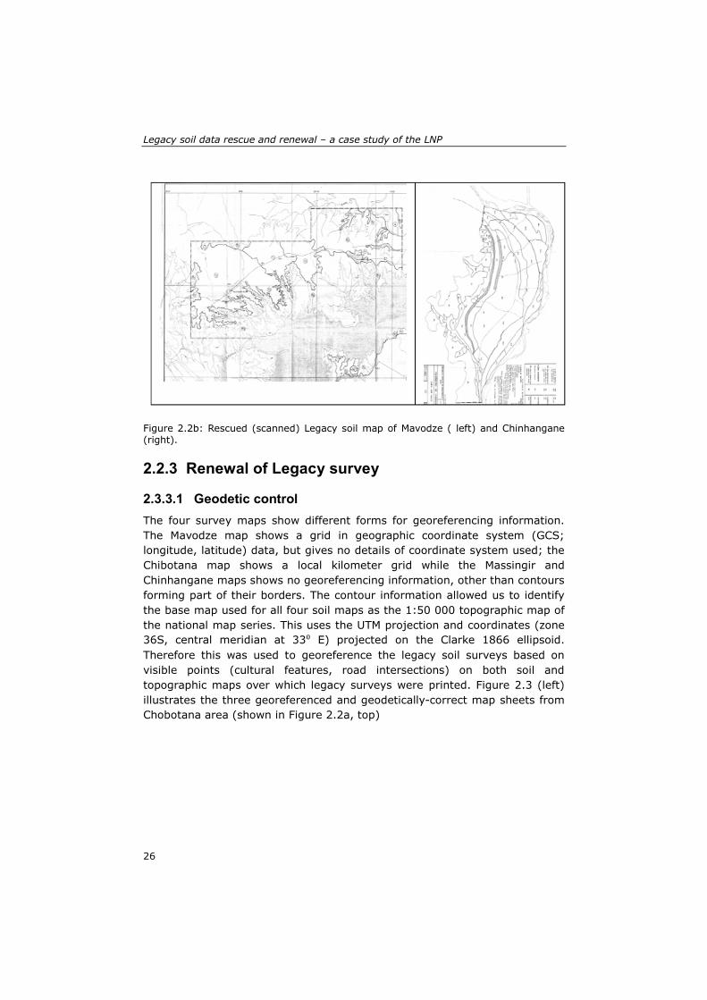
Figure 2.2b: Rescued (scanned) Legacy soil map of Mavodze ( left) and Chinhangane (right).
2.2.3 Renewal of Legacy survey
2.3.3.1 Geodetic control The four survey maps show different forms for georeferencing information. The Mavodze map shows a grid in geographic coordinate system (GCS; longitude, latitude) data, but gives no details of coordinate system used; the Chibotana map shows a local kilometer grid while the Massingir and Chinhangane maps shows no georeferencing information, other than contours forming part of their borders. The contour information allowed us to identify the base map used for all four soil maps as the 1:50 000 topographic map of the national map series. This uses the UTM projection and coordinates (zone 36S, central meridian at 33⁰ E) projected on the Clarke 1866 ellipsoid. Therefore this was used to georeference the legacy soil surveys based on visible points (cultural features, road intersections) on both soil and topographic maps over which legacy surveys were printed. Figure 2.3 (left) illustrates the three georeferenced and geodetically-correct map sheets from Chobotana area (shown in Figure 2.2a, top)
26

Chapter 2
Figure 2.3: Improved geodetic control of combined three legacy soil map sheets of Chibotane soil map (left) and, digitized GIS area-class (soil units) and point (soil profiles location) layers overlaid onto the geodetically correct scan (right). and Table 2.3 shows the quality of improved geodetic control (RMSE) for all selected legacy maps. Despite the RMSE measure be a spatial average and not sensitive to spatial variation in geometric accuracy, it well represents the
27

Legacy soil data rescue and renewal – a case study of the LNP
average error (Hughes et al., 2006). The large number of ground control points (GCP) used in majority of maps, reflects the difficult task to attain a low RMSE. However, even with low RMSE, transformation may still contain large errors due to poorly entered GCPs. Obtaining a necessary large number of GCP was limited mostly due to the poor quality of the legacy map in terms of features that could be easily recognized also on the reference topographic map of the national series. All four surveys showed relative georeferencing RMSE as a substantial proportion of the square root of the MLA (Table 2.3), at best 13% and at worst 45%. So, although the maps could be georeferenced, the geodetic control is poor. Although the transformation errors were minimized by adding more GCPs and replacing those that resulted in increased RMSE, the comparison made of RMSE with the square root of MLA indicates the good co-registration accuracy and as such it serves as a guiding approach to quality legacy data (rescue and) renewal. Table 2.3: Quality of improved geodetic control as assessed by the RMSE of georeferencing. Added are the number of ground control points (GCP), map scale, Maximum location accuracy and Minimum Legible Area (MLA) Legacy Survey
RMSE (m) – 1st order polynomial
Nr GCP
Map scale Maximum location accuracy at scale (m)
MLA [ha]
side length of MLA (m)
RMSE proportion of side length MLA
Mavodze 56.92 20 1:50 000 12.5 10 316.23 0.18 Chibotane 1 10.77 9 1:10 000 2.5 0.4 63.25 0.17 Chibotane 2 26.32 8 1:10 000 2.5 0.4 63.25 0.42 Chibotane 3 8.14 4 1:10 000 2.5 0.4 63.25 0.13 Massingir 28.64 19 1:10 000 2.5 0.4 63.25 0.45 Chinhangane 24.16 12 1:10 000 2.5 0.4 63.25 0.38
2.3.3.2 Area-class and point data GIS coverages Figure 2.3 (left) shows the georeferenced and geodetically correct rescued (scanned) soil map of Chibotane and Figure 2.3 (right) shows GIS coverages of area-class (soil units) and point data (soil profile locations) layers on-screen digitized and overlaid onto the just rescued and georeferenced soil map of Chibotane. The creation of area-class layer was a tedious and time-consuming task of digitizing through the middle of each magnified polyline, as compared to point layers. One way to minimize the tedious work would be the implementation of automated feature extraction algorithms as this would ensure easy, quick and accurately digitized legacy map features. Nevertheless, digitalization was made through the middle of each magnified polyline (and points). In so doing, digitalization should be accurate enough as no sliver fell outside the width (line) or diameter length (point) of scanned map features. In a later stage, features automatically extracted could be used as high accuracy representation against which the positional accuracy of manually digitized features could be assessed. However, in absence of automated feature extraction algorithms, the procedure here followed can be handy to ensure acceptable quality of GIS area-class (and point) layer
28

Chapter 2
creation. Attribute tables of point data layers were populated with profile number, pedological soil unit (FAO 74 legend), A-horizon depth, SOC concentration and Bd (available only in Chinhangane). Attribute tables of area-class maps were populated with soil unit (identification legend), polygon area, A-horizon depth, SOC, Bd and SOC stocks. Apart from map unit code and area, all other data was retrieved from the point data layer by point-in-polygon identification; multiple points in the same polygon were averaged. Not all polygons contained representative profiles; for these, profile from sampled units with the same identification legend were used. Since the legacy surveys of Chibotane, Massingir and Chinhangane share the same legend, representative profile data was shared over these three survey areas whenever necessary. Finally there were few cartographic units without representative profiles. In those cases, the most similar profile from the same or nearby survey area was used.
2.3.3.3 Quality assessment Given the effort to ensure a good quality in data capture, the quality of rescued legacy maps in evaluated next, mainly using the Cornell guidelines (Forbes et al., 1982). Map scale and texture Forbes et al. (1982) recommend a point-count method to estimate ASD on paper maps; however with digital maps direct computation in the GIS is immediate and precise. The summary of delineation sizes of Massingir legacy survey are shown in Figure 2.4 from which it is that clear most delineation sizes range between 5 and 15 ha. Table 2.4 shows the MLA and IMR for the area-class coverages. All delineations of all surveys are larger than the MLA, which indicates that the legacy soil maps meet the standard in this regard. However, all IMR are well above the recommended threshold value (2.0), meaning that legacy maps are legible but could be substantially reduced before losing legibility. It seems that strategically would be better to draw renewed maps following map scale and texture analysis prior to the choice of the final map scale. The optimum scale could thus be reduced by the IMR, which would result in a scale of about 1:1 350 000 (Mavodze), 1:110 000 (Massingir), 1: 150 000 (Chibotane) and 1:90 000 (Chinhangane). Clearly the intensity of survey information does not support the advertised scales. Some of this may be due to large areas of homogeneous soils at the chosen categorical level; in this case the categorical level could have been reduced to show finer distinctions (e.g., by establishing soil series or phases) or the map could be reduced.
29

Legacy soil data rescue and renewal – a case study of the LNP
Figure 2.4: Summary of area size of the captured GIS area-class (soil units) layer from Massingir legacy soil survey, further used to assess the index of maximum reduction (IMR). Table 2.4: Assessment of map scale and map texture through the average size delineation (ASD) and Index of maximum reduction (IMR) of selected LNP legacy soil maps.
Soil map Map unit area [ha] Map texture Max Min Mean ASD [cm2] IMR [-]
Mavodze 8650.2 26.1 1438.7 287.7 26.8 Massingir 1384.7 0.8 51.5 51.5 11.3 Chibotane 310.9 2.1 84.8 84.8 14.6 Chinhangane 266.1 0.6 30.5 30.5 8.7
Map legend Table 2.5 show samples of soil map legend of the four survey areas, summarizing map unit information whose structure forms the map unit definition criterion. All four legends are based on a mixture of air-photo interpretation (physiographic elements) at higher levels and pedological aspects at lower level. The general description of soils in each map unit is included in the report, in most cases along with representative profiles.
30

Chapter 2
Table 2.5: Samples of soil map legend tables of Mavodze, Massingir, Chibotane and Chinhangane
(1) Rooting depth; (2) Texture class; 2.1 Surface; 2.2 Subsurface; (3) CU water; (4) Permeability; (5) Salinity; (6) Sodicity In the Mavodze soil survey, map unit definition criteria consider (1) the physiographic units A, B1-3, C1-3 (which are also the cartographic units’ symbols) and, (2) association of FAO/Unesco 74 soil units. The two aspects are linked as follows: physiographic unit “A” was assigned to eutric + calcaric Fluvisols, “B1” to haplic + luvic Xerosols, “B2” to the haplic + luvic Xerosols (with or without petric phase), “C1” to Ferralic Arenosols, “C2” to Ferralic Arenosols with petric phase, “C3” to luvic Xerosols (with or without petric phase) plus ferralic Arenosols (with petric phase). “B3” was linked to the heavily petrified and to all uncharacterized soils. The pedological soil units were derived based on soil profile information. The legend table of soil maps of Chinhangane, Chobotane and Massingir (Table 2.5), all at 1:10 000 scale, share the same legend, despite the slight differences in their structures. The most detailed legend is that of Massingir,
Mavodze (1:50 000), 1983 Cartographic Unit Physiography Dominant soils A Alluvial plains of Singuidzi River Eutric Fluvisols (Je)
Calcaric Fluvisols (Jc) B B1 B2
Sloping and undulating sedimentary areas from the Tertiary Colluvial lowlands and adjacent gentle slopes Undulating to gently undulating relief
Haplic Xerosols (Xh) Luvic Xerosols (Xl1) Calcic Xerosols (Xk)
Chinhangane (1:10 000), 1982
Physiography Cartographic unit Dominant soils Areal extent ha %
A (Alluvial plain) Aa – Flooding area….
Aa1 Aa2 Aa3
(‘modal’) Eutric Fluvisols Je1 Je2g2,3 Je3g3,4; Je4g3,4
37.4 52.5 57.0
3.2 4.5 4.9
B (Sedimentary zone) Ba – Colluvial lowlands
Ba
Colluvial (Jb) Jb
43.1
3.7
Chibotane (1:10 000), 1983
Cartographic Unit Pedological Unit Areal extent Dominant Sub-dominat ha %
Aa – Flooding área Aa1 Aa2 Ab – Marginal área Ab1 Ab2 Ab3
Eutric Je1
Je3g3,4; Je3 Je1A; Je1 Je2, Je2g2; Je2g3 Je3
Fluvisols (Je) Je1A Je3g; Je2g Je2g Je3; Je3g2; Je3g3 Je4
26.2
153.3
324.7 49.5 67.2
1.2 7.1
15.0 2.3 3.1
Massingir (1:10 000), 1981
Cartog Unit
Geo
Topogra
phy
Drain
Soils Soil characteristics Dom Sub-Dom (1) (2) (3) (4) (5) (6)
(2.1) (2.2) Aa1 Aa2 … Aa6
Aa Less frequent flooding
1 2g2,3 5; 5g3,4
1A; 2v2; 2g2,3 1A; 2v2,3; 2g2,4 3g2,3; 4g; 1A
Ba Bb
Ba Bb
Jb Xv1; Xv2
- Qa; Rm
31

Legacy soil data rescue and renewal – a case study of the LNP
which covers almost all contents of the remainder. It is structured in six main columns, successively populated with cartographic units (Aa1-6, Ab1-6, Ac1-7, Ad1-6 and Ba-b), geomorphology (Aa….Ad, Ba and Bb), topographic characteristics, drainage conditions, soils (dominants and sub-dominants) and soil characteristics (thickness, surficial and sub-surficial texture, available water capacity, soil permeability, soil salinity and sodicity). The first letter of geomorphology unit entry symbols is of the same nature as that of Mavodze physiographic units “A” and “B”, while the second (lowercase) letter is added to indicate the different “geomorphic units” as follows: floodplain area (Aa), Levees (Ab), smoothly sloping slopes of the outer levees side (Ac), back swamps (Ad), colluvium filled lowland “Ba” and the undulating and upper smooth slopes on sediments from Tertiary “Bb”. The topography and drainage entries are descriptive entries of “geomorphology” entry. Under “drainage” the flooding frequency is described instead. The soil entry is populated with sets of dominant + subdominant associations of pedological soil units (FAO/Unesco 74 legend). Similarly to Mavodze, all “A” geomorphologic units are associated to eutric Fluvisols, those under “B” to (colluvial) eutric Fluvisols (Ba) and luvic Xerosols (Bb) soil units. Each set forms also a subdivision of the “geomorphic unit”, which is based on top-soil textures class denoted by a number, next to the Symbol of the FAO/Unesco 74 soil unit as follows: Sandy (1) or loamy sand (1A), sandy loam (2), loam, silt loam or sandy clay loam (3), clay loam or sandy clay loam (4) and silty clay or clay (5). However, this parameter is one of the description aspects under “texture” (see under “soil characteristics” entry referred to earlier). Finally the sub-surficial texture and the depth range in which this layer occurs are denoted by a lowercase letter (h, g, p, v or c) and a number (1, 2, 3, 4 or 5) respectively, added following the top soil texture class of both dominant and sub-dominant soil units. However they are not used as a definition criterion for further distinction of cartographic unit but rather descriptive aspects. Table 2.6 shows the evaluation of map unit definitions. Since map units are associations of pedological units, a map unit was considered to be “well-defined” only if all members had the same positive evaluation result. The inclusion of soil classification in map unit descriptions should have made all units “adequately defined”. However, one could not be confident of names assigned map units that had not been sampled nor contained a representative profile. As such the adequacy criterion “unambiguous placement in a taxonomic class” as suggested by Forbes et al. (1982) was questioned. Therefore, those units were considered “not adequately defined”. The overall information quality of the surveys is “adequate” (>80%) for all surveys when the “proportion/percentage of area-size of “adequately defined” map unit description is considered rather than the “proportion/percentage of number of cartographic units adequately defined”.
32

Chapter 2
Table 2.6: Assessment of map unit definition and overall information quality of soil survey for the selected legacy soil maps from LNP. In between brackets the total number of soil profiles in each survey area
*: no lab data in one soil profile; **: one of them could not have a replacement; A: adequately define, NA: not adequately defined Despite the simplicity of the Mavodze legend from the surveyor point of view, there are few aspects on its structure worth commenting; first, the cartographic unit entry reflects two hierarchical levels (A, B and C; unspecified) and physiography (A, B1-3 and C1-3), which could well be separated in two different hierarchical levels (separate columns), to show the dichotomic subdivision of “unspecified” into physiographic units, since it is clear that, in general the “unspecified” units “A” are associated to Fluvisols, “B1-3 (and C3)” to Xerosols and “C1-2” to Arenosols. Second, there is no indication of the proportions of pedological units forming each association, creating confusion when the same pedological unit appears in a different physiographic unit where it is part of a different association. The proportion of the different members within soil association, and thus its homogeneity, cannot be assessed without additional field work. When legend table is built in a hierarchical approach, lower-level categorical units are easily interpreted within higher categories. The legend structure can thus be improved by (1) separating the “unspecified” from physiography into a different level. Thus it is suggested to name the unspecified hierarchical level to “Land type and position” and, (2) by placing the cartographic units at the end of the legend. Table 2.7.a shows the suggested improvement of Mavosze legend.
Variable Approach Diagnostic criterion
Units Mavodze (nr|ha)
Chibotana (nr|ha)
Massingir (nr|ha)
Chinhagane (nr|ha)
Map unit definition
General map unit information
Unambiguously placeable in a taxonomic class
Cartographic 7 (10) 12 (30) 28 (20) 18 (14)
Total 15 21581.0 24 2035.9 55 2833.1 39 1190.0
A (sampled) 15* 19567.4 15 1816.4 13 2267.7 7 534.0
A (not sampled, with representative profile
8 2013.6 6 154.2 23 334.5 23 490.6
NA (not sampled and no representative profile)
0 0 3 154.2 19** 230.9 9 165.5
Overall information quality
proportion of “adequate” land size
80% or more “adequately defined”
% well defined 100 100 87.5 96.8 65.5 91.8 76.9 86.1
Evaluation A A A A NA A NA A
33

Legacy soil data rescue and renewal – a case study of the LNP
Table 2.7.a: Improved survey legends of Mavodze, after introduction of “Land type and position” entry and repositioning the cartographic unit at the last (third) entry to depict the map definition hierarchal structure.
Land type and position
Physiography Cartographic unit
Dominant soil association
Extent ha %
A - lowlands (flat) 1 (sole unit) A B - intermediate undulating and sloping land
1…3 B1…B3
C - peneplained upper land
1…3 C1…C3
In the Massingir legend table, the terms “geomorphology” and “physiography” were used unnecessary, since the content under “geomorphology” rather reflects that of “physiography” in other legend tables. The columns “topographic characteristics” and “drainage” were used to describe the content of the column ”geomorphology”, rather than to define levels of “geomorphology”. This is also confusing when there is a separate set of columns used to describe the map units at the end of the legend table. Similarly the use of surficial texture class both as definition criteria and map unit description is confusing. The FAO/Unesco 74 legend used in this survey is outdated. This was revised in 1997 (FAO et al., 1997), at which time the major soil grouping of Xerosols was eliminated, since climate was no longer considered a soil classification criterion; most Luvic Xerosols were reclassified as Orthic Luvisols but the Haplic Xerosols could be Regosols or Cambisols depending on the presence of a cambic horizon. Both FAO legends have been superseded by the World Reference Base for Soil Classification (WRB, 2006) which has similarities to the 1997 legend but introduces new concepts, so that for a proper renewal all legacy map units should be reclassified from profile descriptions, supplemented if necessary with inferences from the 1974 names. Improvements to the Chinhangane, Chibotane and Massingir are suggested in Table 2.7b where the hierarchical map unit definition as well as general description of the cartographic units is made. Table 2.7b: Restructured and unified (improved) legend (Massingir, Chibotane and Chinhangane) after inclusion of “Land type and position” and re-positioning the surficial soil texture as part of map unit definition criteria
Land type and position
Physiography & flooding frequency
Top-soil texture
Cartographic unit
Soil association Description Extent Dominant Sub-
dominant ha %
A Aa 1 Aa1 Je1 Je1A,… … … 6 Aa6
Ab 1…6 …. …. …. …. Ae 1 & 2 ….
B Ba - Ba
34

Chapter 2
2.3.3.4 Integration of RS and DEM layers The 100 masl and 90 masl contours were used as the southern (Massingir) and western (Chinhangane) borders, respectively, in two surveys. These contours as shown on the georeferenced digitization of the published maps were compared to those derived from the SRTM DEM. Figure 2.5 (left) shows The 100 and 110 masl derived contours overlaid onto the Massingir soil map GIS coverage. Similarly, the 90 masl contours is shown (Figure 2.5, right) overlying the Chinhangane soil map GIS coverage.
Figure 2.5: The 100 and 110 masl contours extracted from SRTM DEM overlaid onto Massingir soil map (left) and the 90 masl contour overlaid onto Chinhangane soil map (right), whose southern (Massingir) and western (Chinhangane) borders were considered to be 100 and 90 masl contours, respectively. From this comparison, it is clear there is a large mismatch between the drawn and SRTM DEM derived 100 masl contours. The drawn 100 masl is much closer to the 110 masl SRTM DEM derived contour than the 100 masl one. This casts doubt on the accuracy of all other lines drawn on the map. The 110 and 90 masl SRTM DEM derived contours assumed to be accurate, against which the 100 and 90 masl soil map borders were compared (Table 2.8). The tested length spanned between two crossing points between the contour and soil map border and, in the absence of local map accuracy standards, the maximum location accuracy (2.5 m for 1:10 000 legacy soil map scale) was used to start the iteration as suggested by Goodchild and Hunter (1997). Linear interpolation in results (Table 2.8), show that less than 30% of border length (both cases) falls within a buffer length of the square root of MLA, thus the positional accuracy is poor. Only at a buffer length of 348.7 m all the tested Chinhangane’s border falls in while only about 90% of Massingir falls in for similar buffer length (320.5 m). Therefore, replacing the mapped soil borders by their high accuracy representation from contours
35
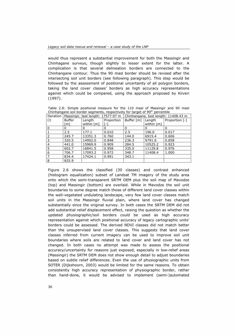
Legacy soil data rescue and renewal – a case study of the LNP
would thus represent a substantial improvement for both the Massingir and Chinhagane surveys, though slightly to lesser extent for the latter. A complication is that several delineation borders are connected to the Chinhangane contour. Thus the 90 masl border should be revised after the intersecting soil unit borders (see following paragraph). This step would be followed by the assessment of positional uncertainty of all polygon borders, taking the land cover classes’ borders as high accuracy representations against which could be compared, using the approach proposed by Kiiveri (1997). Table 2.8: Simple positional measure for the 110 masl of Massingir and 90 masl Chinhangane soil border segments, respectively for target of 99th percentile Iteration (i)
Massingir, test length: 17577.97 m Chinhangane, test length: 11408.43 m Buffer [m]
Length within [m]
Proportion [-]
Buffer [m] Length within [m]
Proportion [-]
0 0 0 0 0 0 0 1 2.5 177.1 0.010 2.5 196.0 0.017 2 245.7 13351.3 0.760 144.0 6915.4 0.606 3 320.5 14902.0 0.848 236.3 9791.6 0.858 4 441.0 15969.9 0.909 284.5 10525.2 0.923 5 602.7 16841.5 0.958 335.0 11129.8 0.976 6 706.7 17093.2 0.972 348.7 11408.4 1.000 7 834.4 17424.1 0.991 343.1 8 825.9 Figure 2.6 shows the classified (30 classes) and contrast enhanced (histogram equalization) subset of Landsat TM imagery of the study area onto which the semi-transparent SRTM DEM plus the soil map of Mavodze (top) and Massingir (bottom) are overlaid. While in Mavodze the soil unit boundaries to some degree match those of different land cover classes within the well-vegetated undulating landscape, very few land cover classes match soil units in the Massingir fluvial plain, where land cover has changed substantially since the original survey. In both cases the SRTM DEM did not add substantial relief displacement effect, raising the question as whether the updated physiographic/soil borders could be used as high accuracy representation against which positional accuracy of legacy cartographic units’ borders could be assessed. The derived NDVI classes did not match better than the unsupervised land cover classes. This suggests that land cover classes inferred from current imagery can be used to improve soil unit boundaries where soils are related to land cover and land cover has not changed. In both cases no attempt was made to assess the positional accuracy/uncertainty for reasons just exposed, especially in low-relief areas (Massingir) the SRTM DEM does not show enough detail to adjust boundaries based on subtle relief differences. Even the use of physiographic units from SOTER (Dijkshoorn, 2003) would be limited for the same reasons. To obtain consistently high accuracy representation of physiographic border, rather than hand-done, it would be advised to implement (semi-)automated
36

Chapter 2
procedure similar to e.g. terrain analysis by Gallant and Wilson (1996), supervised landform classification by Hengl and Rossiter (2003), and automatic segmentation of landforms by MacMillan et al. (2000). However they should be much more sensitive to subtle relief differences. The resulting physiographic units’ borders could be used to assess the positional accuracy of legacy maps.
2.3.3.5 Metadata Following step by step of the ArcCatalog 9.2 metadata editing process, most of the template form were populated, especially those refereeing to Identification information, spatial reference, entity attribute and data quality. Table 2.9 shows some of the (xml document file) metadata included in the GIS layer of Massingir renewed legacy soil map. This information should allow others users to access the data and evaluate its usefulness for their intended purposes.
37

Legacy soil data rescue and renewal – a case study of the LNP
Figure 2.6: The Mavodze (top) and Massingir (bottom) soil maps overlaid onto Landsat TM classified (unsupervised) image
38
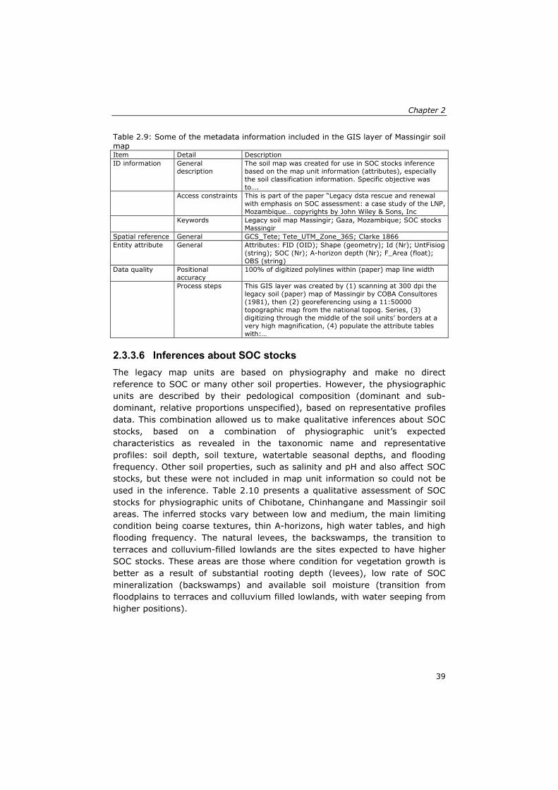
Chapter 2
Table 2.9: Some of the metadata information included in the GIS layer of Massingir soil map Item Detail Description ID information General
description The soil map was created for use in SOC stocks inference based on the map unit information (attributes), especially the soil classification information. Specific objective was to….
Access constraints This is part of the paper “Legacy dsta rescue and renewal with emphasis on SOC assessment: a case study of the LNP, Mozambique… copyrights by John Wiley & Sons, Inc
Keywords Legacy soil map Massingir; Gaza, Mozambique; SOC stocks Massingir
Spatial reference General GCS_Tete; Tete_UTM_Zone_36S; Clarke 1866 Entity attribute General Attributes: FID (OID); Shape (geometry); Id (Nr); UntFisiog
(string); SOC (Nr); A-horizon depth (Nr); F_Area (float); OBS (string)
Data quality Positional accuracy
100% of digitized polylines within (paper) map line width
Process steps This GIS layer was created by (1) scanning at 300 dpi the legacy soil (paper) map of Massingir by COBA Consultores (1981), then (2) georeferencing using a 11:50000 topographic map from the national topog. Series, (3) digitizing through the middle of the soil units’ borders at a very high magnification, (4) populate the attribute tables with:…
2.3.3.6 Inferences about SOC stocks The legacy map units are based on physiography and make no direct reference to SOC or many other soil properties. However, the physiographic units are described by their pedological composition (dominant and sub-dominant, relative proportions unspecified), based on representative profiles data. This combination allowed us to make qualitative inferences about SOC stocks, based on a combination of physiographic unit’s expected characteristics as revealed in the taxonomic name and representative profiles: soil depth, soil texture, watertable seasonal depths, and flooding frequency. Other soil properties, such as salinity and pH and also affect SOC stocks, but these were not included in map unit information so could not be used in the inference. Table 2.10 presents a qualitative assessment of SOC stocks for physiographic units of Chibotane, Chinhangane and Massingir soil areas. The inferred stocks vary between low and medium, the main limiting condition being coarse textures, thin A-horizons, high water tables, and high flooding frequency. The natural levees, the backswamps, the transition to terraces and colluvium-filled lowlands are the sites expected to have higher SOC stocks. These areas are those where condition for vegetation growth is better as a result of substantial rooting depth (levees), low rate of SOC mineralization (backswamps) and available soil moisture (transition from floodplains to terraces and colluvium filled lowlands, with water seeping from higher positions).
39

Legacy soil data rescue and renewal – a case study of the LNP
Table 2.10: Inference of SOC stocks based on physiographic map unit characteristics Unit Physiographic characteristic Inferences
Location Texture A-horiz. depth
Water dynamic (water level, flooding frequency)
SOC concentration
SOC stocks
Aa Flooding area, between natural levees
coarse deep High watertable, frequent flooding
low low
Ab Natural levee medium deep deep watertable, no flooding
medium medium
Ac Outer gently sloping levee slopes (occurrence of oxbow lakes)
medium deep deep watertable, no flooding
Low low
Ad Backswamps Fine deep High level, frequent flooding
medium medium
Ae Outer edge flood plain, rich in water ways
Medium deep High level, moderate flooding
medium medium
Ba Colluvium filled lowlands (sediments from Tertiary and Quaternary)
medium deep Deep, rare flooding medium medium
Bb Erosional/undulating upper terraces (Tertiary and Quaternary), under dense mopane
Coarse shallow deep watertable, no flooding
medium low
T Upper terraces under dense mopane
Coarse shallow deep watertable, very rare flooding
medium low
Section 2.3.3.2 presented the point data layers with attribute tables populated, amongst others, by the SOC concentration, A-horizon thickness and Bd. Data from 64 soil profiles were available. Figure 2.7 shows the summary SOC data, ranging mainly between 0.4 and 1.4%, well within the range of mean SOC (A-horizon) per survey area (Table 2.10). This range is within the range of mean SOC spatial distribution predicted for the entire LNP (Cambule et al., 2013). These low values are expected, due to the substantial coarse textured soils in the study area and the hot dry climate.
40

Chapter 2
Figure 2.7: Summary of retrieved SOC concentration data from legacy soil profiles data of Mavodze, Massingir, Chibotane and Chinhangane. Table 2.11 also shows the computed SOC stocks for each the four survey areas, following the measure and multiply approach (Thompson and Kolka, 2005). The range of area-normalized mean SOC stocks is 2.0 – 4.0 kg m-2. These values are a little higher than those found by Cambule et al. ((under review)) and, given the fact that SOC concentration is comparable to those across the LNP, the higher mean SOC stocks may be explained by the thicker A-horizons typical of floodplain soils. The computed stocks are also higher than those found by Vågen (2005) for southern African soils, but far lower than those found by Ryan et al. (2011a) and also at the lower end of those obtained by Williams (2008) in an eastern miombo woodlands in Mozambique. These higher stocks are likely due to the high litter leaf from the leguminous trees (Brachystegia spiciformis) which is typical of miombo woodlands. Table 2.11: Inference of SOC stocks in A-horizon of legacy soil survey areas based on available point data
Variable Units Legacy soil survey area Mavodze Massingir Chibotane Chinhangane
Bd mean Ton Kg-1 1.4 1.4 1.4 1.4 A_depth mean m 0.24 0.25 0.31 0.28 SOC mean % 0.46 1.12 1.01 0.75 Total Area km2 215.8 28.3 20.4 11.9 SOC Stocks ton 413260.2 70432.9 78796.3 33764.4 SOC Stocks mean Kg m-2 1.9 2.5 3.9 2.8
41

Legacy soil data rescue and renewal – a case study of the LNP
The total SOC stocks of the four survey areas is 596.2 Gg, which represents about 4.0% LNP stocks (16744 Gg) estimated by Cambule et al. ((under review)). This is proportionally about the same since the study area is 276.4 km2, about 3% of LNP area size. The small area-size and especially the not so representative floodplain type of the physiography covered by legacy data, limits its extrapolation to the whole LNP. The SOC stocks just inferred are reflect the soil conditions in the early 1980s and might not accurately represent the current situation due to changes in factors controlling the dynamic of SOC stocks, e.g. land use. Vågen (2005) reported SOC stocks change rates of about -0.82 ton C ha-1 yr-1 in southern Africa after conversion from savanna to agriculture and of about -14.26 ton C ha-1 yr-1 from woodlands to agriculture in the east Sudanian savanna. In Masvingo (Zimbabwe), Zingore et al. (2005) modelled long-term change rate of about -0.26 ton C ha-1 yr-1 for woodlands clearance for smallholder subsistence farming; this is closer to the situation of LNP study area.
2.4 Summary and Conclusion Below follows the summary of this study with respect to stated objectives. The data archaeology exercise was successful, and revealed many more relevant surveys than was initially suspected when beginning the project. Similar diligent detective work in any area of the world is likely to uncover a large number of useful surveys. The renewal of selected surveys was possible to some extent. It was not possible to solve problems of missing information, nor rectify map unit boundaries not defined according to physiography or land cover which could be identified on recent imagery and DEM. It was possible to identify base maps and their original geometry, and thus georeference the soil maps to moderate accuracy. Each step was documented, as well as what was possible to infer about the source maps, as systematic metadata in the renewed digital products. It was possible to assess data quality for SOC mapping and monitoring, and make semi-quantitative estimates of the spatial distribution of SOC stocks at the mapping dates. This exercise revealed that the effective map scales as measured by the IMR and observation density were much smaller than publication scales. The Cornell adequacy criteria proved to be a useful framework for determining the fitness for use of legacy surveys. The advances in GIS since the original publication (1982) enabled the computation of geodetic and scale adequacy exactly more efficiently than in the original proposal.
42

Chapter 2
To conclude, the strategies for the renewal of legacy soil data here followed can be applied in general, whether to get the maximum value out of legacy surveys or to identify spatial and thematic knowledge gaps to guide (partial) resurveys.
43

Legacy soil data rescue and renewal – a case study of the LNP
44

Chapter 3 A DSM methodology for poorly accessible area2
2 This chapter is based on: Cambule, A.H., Rossiter, D.G., Stoorvogel, J.J., 2013. A methodology for digital soil mapping in poorly accessible areas. Geoderma 192, 341-351.
45

A DSM methodology for poorly accessible area
Abstract Effective soil management requires knowledge of the spatial patterns of soil variation within the landscape to enable wise land use decisions. This is typically obtained through time-consuming and costly surveys. The aim of this study was to develop a cost-efficient methodology for digital soil mapping in poorly-accessible areas. The methodology uses a spatial model calibrated on the basis of limited soil sampling and explanatory covariables related to soil-forming factors, developed from readily available secondary information from accessible areas. The model is subsequently applied in the poorly-accessible areas. This can only be done if the environmental conditions in the poorly-accessible areas are also found in the accessible areas in which the model is developed. This study illustrates the methodology in an exercise to predict soil organic carbon (SOC) concentration in the Limpopo National Park, Mozambique. Readily-available secondary data was used as explanatory variables representing the soil-forming factors. Conditions in the accessible and poorly-accessible areas corresponded sufficiently to allow the extrapolation of the spatial model into the latter. The spatial variation of SOC in the accessible area was mostly described by the sampling cluster (71.5%) and the landscape unit (46.3%). Therefore ordinary (punctual) kriging (OK) and kriging with external drift (KED) based on the landscape unit were used to predict SOC. A linear regression (LM) model using only landscape stratification was used as control. All models were independently validated with test sets collected in both accessible and poorly-accessible areas. In the former the root mean squared error of prediction (RMSEP) was 0.42-0.50% SOC. The ratio between the RMSEP in the poorly-accessible and accessible areas was 0.67-0.72, showing that the methodology can be applied to predict SOC in poorly-accessible areas as successful as in accessible areas. The methodology is thus recommended for areas with similar access problems, especially for baseline studies and for sample design in two-stage surveys.
46

Chapter 3
3.1 Introduction Effective land management depends on knowing the spatial distribution of soil properties. Traditionally this knowledge is represented as soil maps conforming to the discrete model of spatial variation; DMSV (Heuvelink and Webster, 2001), showing polygons within which soils are considered homogeneous and with boundaries where changes in soil properties are considered to be abrupt. However, many soil properties can be better modelled with a continuous model of spatial variation (CMSV), in which properties vary continuously in space. The recent rapid development of information technology along with the availability of new types of secondary data (e.g., digital elevation models and satellite imagery) allow for more quantitative approach to soil survey producing continuous surfaces based on soil forming factors. Furthermore, these methods give spatial estimates of the uncertainty of the predictions. This “predictive” (Scull et al., 2003) or “digital” soil mapping (McBratney et al., 2003) uses relationships between soil properties and auxiliary data at sample points to predict over a study area. in addition, the high sampling costs can be reduced by applying recent developments in the field of diffuse reflectance spectroscopy (e.g. Near-Infrared spectroscopy), a fast, non-destructive and inexpensive soil analysis method that can enhance or replace traditional laboratory methods (Shepherd and Walsh, 2002; Viscarra-Rossel and McBratney, 2008). Digital soil mapping (DSM) techniques have been successfully applied in studies at field scale where soil variability is largely due to the effect of topography on soil genesis (e.g., Florinsky et al., 2002) and therefore much of the success is attained by integration of terrain attributes as auxiliary data. To capture the spatial structure of soil variation as well as the soil-environment relations over larger poorly-accessible areas due to poor road networks (such as much of Africa) or difficult terrain (e.g., mountainous regions), a large number of observations following a sound sampling design, covering the feature and geographic space of the predictors (e.g., Minasny and McBratney, 2006) are required, which is impractical or prohibitively expensive. A DSM approach which can concentrate sampling in accessible areas, yet deliver results of sufficient quality, would greatly reduce costs and survey effort. The objective of present study was to develop a methodology for DSM for poorly accessible areas. It consists in developing a quantitative predictive model based on limited sampling (mainly in accessible areas) combined with readily-available auxiliary spatial data representing soil forming factors. It is hypothesized that if the auxiliary data in accessible and inaccessible areas are sufficiently similar, models built in the former can be applied in the latter, with very few or even no soil samples. It is thus applicable in mapping projects where legacy samples from accessible areas are available.
47

A DSM methodology for poorly accessible area
3.2 Material and methods The proposed method is based on similarities between accessible and poorly-accessible areas in terms of the relation between soil-forming explanatory variables (covariables) and soil properties (target variables). If the areas are similar, the predictive model based on soil samples and explanatory variables from accessible areas can be applied in inaccessible areas. The predictive model uses the conceptual model scorpan-SSPFe proposed by McBratney et al. (2003) and widely-applied as a generic method for DSM. Scorpan represents the list of soil-forming factors that has been expanded from the original definition by Jenny (1980) representing the initial soil conditions (s), climatic conditions (c), organisms (o) including animals, land cover and human occupation; relief (r), parent material (p), age (a), and the neighbourhood (n). The conceptual model uses a soil spatial prediction function with spatially-autocorrelated errors (SSPFe) that uses (1) a prediction based on environmental covariables and (2) a prediction based on soil properties measured at a limited set of observation points. This section explains stepwise the proposed methodology as illustrated in the flowchart of figure 3.1 and the way it was operationalized for the specific objectives and context of the test case (The LNP).
48

Chapter 3
Figure3.1: Flowchart of the proposed methodology for digital soil mapping in poorly accessible areas. Step 1: Gathering of secondary data covering all area The secondary data is the raw material to derive insight in the soil forming factors. The data must cover the area of interest (i.e., have values at all locations). A good example is a digital elevation model that covers the area and provides insight in the soil forming factor “relief” (r).
49

A DSM methodology for poorly accessible area
In the test case, the selected secondary data for SOC prediction in LNP included (1) mean annual precipitation at a 30 arc-second resolution grid from the WorldClim website (Hijmans et al., 2011), (2) the multispectral Landsat TM satellite imagery at a 30 m resolution for a wet and dry season from the US Geological Survey website (www.usgs.gov, row/path: 168/076 from August 2009, preprocessing: L1T level), (3) a digital elevation model at a 3 arc-second (approximately 90 m) resolution from the shuttle radar topographic mission (SRTM) from the Jet Propulsion Laboratory (www.jpl.nasa.gov, tile: 43_17, preprocessing: research grade), (4) a 1:250.000 lithology map developed by the Geological Survey of Finland (Manninen et al., 2008; Rutten et al., 2008), and (5) the 1 : 1.000.000 scale landscape map of Stalmans et al. (2004) as an integrated soil forming factor. These latter two are equivalent to, at best, 125 m and 500 m resolution, respectively (Hengl, 2006, Sec. 2.1), the latter somewhat smaller than the largest cluster dimension, 720 m. However, considering the size of the study area, it was decided on a 1 Km resolution (thus, about 10 000 pixels) for the final maps. Step 2: Explanatory variables The gathered secondary data must then be converted into covariables with direct link to soil formation. The Scorpan approach aims to elucidate quantitative relationships between soil properties and the soil-forming factors. The covariables should provide information on soil formation. If covariables describing relevant soil formation processes are lacking the predictive power of the model will be limited. An example is the conversion of a DEM into terrain derivatives such as a wetness index and potential erosion rates (Gessler et al., 2000b; McKenzie et al., 2000). At this stage coverages were derived from the available secondary maps with potential covariables for the test case. The scorpan-SSPfe modelling framework was used to organize the coverages by soil-forming factor. Spatial resolution was kept the same as of the original coverages as it is meant for similarity analysis. The time factor was assumed constant for the present study and therefore no analysis were performed. Climate (c) influences rates of vegetative growth and turnover of soil organic matter through differences in precipitation, temperature and evaporation (McBratney et al., 2003). The most influential organisms (o) for SOC are vegetation and humans (McBratney et al., 2003). The LNP was long used as a hunting zone since colonial times. Later (in 2001) it was declared a conservation area with minimal human influence is minimal, with confined to scattered subsistence farming near the Singuedzi River. Wildlife density is low, and therefore
50

Chapter 3
vegetation is the principal organism related to SOC. Normalized vegetation index (NDVI) is a surrogate of vegetation biomass (whose decay contributes to SOC) and is calculated as (NIR-G)/(NIR+G) where NIR and G are the reflectances in the near-infrared and green electromagnetic spectrum, respectively. Green NDVI is sensitive to chlorophyll concentrations, adequately measuring the rate of photosynthesis (Gitelson and Merzlyak, 1998; Yoder and Waring, 1994), and can therefore be used as an indicator of vegetation cover. Focal statistics at 3x3 pixels were applied to the NDVI grid in order to match the spatial resolution of NDVI with the support of the sample sites. Dry-season NDVI is an indicator of water availability and hence biological activity in that season. Wet-season NDVI is an indicator of maximum vegetative growth. NDVI for the wet (February) and dry (June) seasons were selected to represent the soil forming factor organism in agreement with the study of Mora-Vallejo et al. (2008) in Kenya. Wet and dry season NDVI are derived from Landsat TM scenes that cover most of park. Relief (r) influences water movement and accumulation across the landscape. As a result, relief has indirect consequences on SOC contents through biomass production, erosion, sedimentation and redox conditions. Altitude and flow accumulation (an indirect way of measuring drainage area) were selected as appropriate covariables. Flow accumulation was derived from the DEM using ArcGIS 10. Values above 50 pixels are excluded as they correspond to drainage lines. Parent material (p) was represented by the lithology map. Small units were merged with neighboring larger ones of similar lithology to avoid a large number of different units. The spatial factor (n) accounts for spatial trends not revealed by other factors (McBratney et al., 2003). Although in principle any trend should be reflected by the soil forming factors, the selected covariables may not capture all the regional variation. Hence the spatial position was represented by the coordinates. The soil factor (s) represents soil attributes measured at sampling locations. The SOC concentrations derived from a Partial Least Square Regression (PLSR) calibration model relating the Near-infrared spectral signature of a soil sample to its SOC concentration (%) was used. Field sampling and laboratory analysis details are described further on. Finally, the advantage of the landscape study of Stalmans et al. (2004) was taken to consider the landscape units as an integrated soil-forming factor, combining elements of lithology, general relief, climate, and soil type into a
51

A DSM methodology for poorly accessible area
local eco-region. Stalmans et al. (2004) classified LNP into ten major landscape units, as summarized in the study area description. Step 3: Stratification of study area At this stage the study area should be divided into accessible (ACC) and poorly-accessible (PACC) areas. The latter are those beyond easy reach by common means due to, for example, poor road infrastructure, difficult navigation, wildlife hazard, or poor security. The main road network, comprised of two dirt roads following the N-NW direction, one along the right margin of the Limpopo River, and the other located about the centre of the park, along Singwedzi River (parallel to the Limpopo River) was mapped using a handheld GPS while traversing the entire network in an all-terrain vehicle. This included few other roads connecting main roads. The areas within 2.5 km of a road were considered accessible areas. This threshold was considered a practical limit of easy access for field sampling (including carrying tools, water, samples, and a firearm for protection against wildlife) after parking a vehicle along the road. Step 4: Assessment of similarity between strata At this stage ACC and PACC strata must be compared to evaluate the degree to which conditions in PACC areas are found in the ACC areas. This determines the potential applicability of the methodology. Similarities can be assessed by comparing, e.g., the histograms, ranges, clusters, class frequencies, or trends of covariables between the two areas, either qualitatively or with formal similarity measures. A decision is taken as to whether PACC areas are sufficiently represented by ACC areas; if not, the method is not applicable and both areas need to be sampled. In the test case the similarity between the two areas was evaluated by comparison of the mean and the inter quartile range (IQR) for the quantitative covariables and the proportion in which each mapping unit occur in ACC and PACC areas for the categorical covariables. It would have been instructive to do this comparison per-stratum; however, this requires an adequate number of grid cells in each stratum for both ACC and PACC areas. In the present study this was not possible because of the small area of some combinations, e.g., there were only 34 grid cells in the ACC area of the CMR stratum. Step 5: Sampling of accessible areas, laboratory analysis and PLSR-NIR calibration model A sampling strategy must be designed and implemented to gather a representative sample of the target soil properties in ACC areas. The sampling strategy should be based on the available information from the
52

Chapter 3
covariables (Minasny and McBratney, 2006), the expected spatial structure (Lark, 2002; Webster et al., 2006), or a combination (Brus and Heuvelink, 2007). If there are legacy samples, and if these can be harmonized with current methods, they can be used to optimize the sampling plan, e.g., by simulated annealing (Brus et al. 2007). The only legacy soil observations in the LNP are from a 1969 irrigation suitability survey of the extreme SE of the park, with poor georeference and no analytical data. Therefore the sampling design did not take these into account, and started from the “no previous data” situation. Accessibility and wildlife hazard were major constraints to a random or regular sampling design. Therefore a stratified, clustered random sampling design was applied, which provides a statistical valid sample with high operational efficiency (De Gruijter et al., 2006). The LNP was stratified by landscape units (Stalmans et al., 2004), this being an integrative factor of soil genesis, and so is expected to capture a large part of the SOC variation. The number of clusters per stratum, i.e., landscape unit, was proportional to the stratum size. Sixty clusters were planned, 46 for model calibration in accessible areas and 14 for validation across LNP. Both sets were collected in the same field campaign. Cluster centres were positioned randomly within each stratum. Each cluster was composed out of two orthogonal transects of 720 and 360 m length crossing at their midpoints with a total of 7 sampling points units 180 m apart (Figure 3.4). In order to capture the maximum variation the longer transect was oriented along the aspect as determined at the midpoint. At each sample point one soil sample was collected and this was a composite of five sub-samples from the four corners of a 90 m square support area plus the centre. Each sub-sample was from a (variable-thickness) field-identified (and measured) A horizon, collected with a hand shovel after scooping out the upper 2-5 cm (to remove sticks, undecomposed leaves, etc). Subsamples were thoroughly mixed in a bucket, and then about a half a kg was collected in a plastic bag and sent to soil laboratory. In order to minimize the costs of laboratory analysis, all samples were analyzed using NIR spectrometry and a PLSR-NIR calibration model relating SOC to NIR spectra was built and validated (chapter 4) as described in Cambule et al. (2012). The PLSR predicted SOC was then used as explanatory variable for the “soil” (s) factor. Step 6: Building of spatial model for accessible areas The correlation between explanatory variables (i.e., the environmental covariables) and the soil properties of interest must be evaluated, using pedometric modeling approaches (McBratney et al., 2003; McBratney et al., 2000) to build a quantitative model for the accessible areas. A separate
53

A DSM methodology for poorly accessible area
model must be built for each property. The model may include local spatial correlation, e.g., regression kriging (Hengl et al., 2007), but since the PACC area is by definition not or very sparsely sampled, the local spatial structure cannot be used to explain much of the variability in these areas. The calibrated model must be applied to the environmental covariables and measured soil properties to make a prediction map of the soil properties of interest across ACC areas. This should also produce an estimate of the prediction variance as an internal measure of model quality. In the test case the spatial model for ACC was developed on the base of explanatory variables that best explain SOC variation, for which appropriate spatial models were selected, followed by spatial structure (within- and between-cluster) analysis, as follows: To assess the proportion of SOC variation explained by the continuous explanatory variables, pixel values of each explanatory variable layer at sampling points were extracted and regressed against SOC; the regression model was evaluated by ANOVA of the model compared to a null model, and by visual inspection of regression diagnostic plots (Fox, 1997). The proportion of SOC variation explained by the categorical explanatory variables (clusters, geology and landscape) was evaluated by means of ANOVA of linear models of SOC as a function of each categorical variable. Regression adjusted goodness-of-fit was used to select explanatory covariables for model building and the appropriate spatial prediction model. Residuals from selected models show the unexplained variation in SOC. These, as well as the original values of SOC, were examined for local spatial autocorrelation using empirical variograms (Goovaerts, 1999). If structure was evident, models of spatial dependence (both original values and model residuals) were fit to the empirical variogram using weighted least square (WLS) in gstat (Pebesma, 2004). Anisotropy was evaluated visually with a variogram map. In order to minimize irregularities (due to small sampling size and to avoid arbitrary decisions on variogram bin width) and therefore improve the variogram fitting within the range of the variogram model, a residual maximum likelihood (REML) (Marchant and Lark, 2007) was applied directly to the variogram cloud from WLS fit, using gstat. The ordinary and residual variogram with spherical models using all calibration samples was fitted. In order to assess within-cluster spatial autocorrelation, an experimental variogram spanning the cluster range (720 m) was calculated, plotted and visually inspected in order to determine the practical support area, within which SOC variation is controlled by very short-range factors (i.e., within a cluster) and therefore should be ignored when mapping.
54

Chapter 3
SOC was predicted across ACC areas from the calibration observations, by applying the selected spatial models. Internal prediction quality was assessed by kriging prediction standard deviation (Goovaerts, 1999; McBratney et al., 2000). Step 7: Validation of spatial model in accessible areas At this stage an independent field sample must be taken, using the same strategy as the calibration sample; for practical reasons this could be during the original sampling campaign, with a proportion taken out randomly for this validation. The model prediction must then be compared to the true values with measures of quality such as root mean square error of prediction (RMSEP), or bias and gain of modeled vs. actual. If the model quality does not match requirements, one of the following corrections must be undertaken: (1) try another model structure or explanatory variables; (2) make more observations to refine the model; (3) abandon the DSM project if properties cannot be predicted with this approach. The sampling plan (step 5) considered an independent set for the validation of spatial model. A sub-set comprised by those samples collected in accessible was used for spatial model validation in ACC. Step 8: Application of spatial model in poorly-accessible areas The calibrated model must be applied to the environmental covariables and field-sampled soil properties (from ACC areas) to make a prediction map of the soil properties of interest across poorly-accessible areas. If there is any local spatial structure represented in the model, the prediction quality will naturally be better nearer to ACC areas. SOC was predicted here using the same models and the same support area, also for the same reasons as in the ACC area. The internal prediction quality was also assessed by kriging prediction standard deviation (KPSD) (Goovaerts, 1999; McBratney et al., 2000). Given the rocky nature of the LN and MCM units, their SOC contents were assumed to be effectively zero. Most landscapes in LNP are dominated by plant communities with Colophospermum mopane. However, this mopane vegetation is not present in the aeolian sands (PS) and in wetter (LLF and SAF) landscapes along the major drainage lines. Step 9: Validation of spatial model in poorly-accessible areas An independent field sample using the same strategy as the validation set in ACC must be taken; but this will be by definition quite limited (this is the motivation of the methodology), given the difficulty of access. Validation is as accessible areas and similarly to step 7 where a sub-set of independent validation set comprised of samples collected in poorly-accessible was used.
55

A DSM methodology for poorly accessible area
Step 10: Relative performance of spatial model Finally the relative performance in both ACC and PACC areas is assessed: Validation results in the two areas must be compared; the ratio between the validation RMSE and other validation statistics should then be used to determine the degree of success of the methodology for poorly-accessible areas. The performance in accessible areas should already have been judged adequate (step 7); if the relative performance in poorly-accessible areas was satisfactory, by deduction so will be the absolute performance. If relative performance is too poor, there is no remedy but to conduct a full (expensive) sampling in the poorly-accessible area, following the same scheme that produced a satisfactory result in the accessible areas.
3.3 Results and discussion This section presents and discusses obtained results, for the specific objectives and context of the test case. It illustrates the decisions that must be made, and how they can be justified. All statistical analyses were carried out in the R environment for statistical computing (R Development Core Team, 2011) version 2.12 including geostatistical analyses with the gstat R package (Pebesma, 2004) version 1.0.
3.3.1 Explanatory variables Following the gathering and selection of secondary data for SOC prediction in the LNP, explanatory variables were developed. The summary statistics are presented in Table 3.1. Climate (c): The WorldClim database shows a clear rainfall increase to the south with an annual precipitation difference of approximately 220mm (Figure 3.2). The higher grounds in the SW and NW also show precipitation above 500 mm as it is with the SE corner of the study area. Summary statistics (Table 3.1) show a mean bellow 500 mm, which indicate a rather drier climate. Temperature and evaporation do not vary substantially across the area and therefore were left out. Table 3.1: Summary statistics of the soil-forming explanatory variables in LNP as a whole. Variable unit Min Max Range Mean SD
Elevation m 54 531 477 241 99 Flow accumulation nr. Pixels 0 50 50 4 8.2 NDVI wet season - -1.0 0.69 1.69 0.35 0.13 NDVI dry season - -0.34 0.56 0.91 0.11 0.08 Annual precipitation mm 362 580 218 461 40 The most influential organisms (o) for SOC are vegetation and humans (McBratney et al., 2003). Wet and dry season NDVI (Figure 3.2) are derived
56

Chapter 3
from Landsat TM scenes that cover most of park. In general higher NDVI values are found along the main drainage lines and at higher grounds of the northern section along the NNW-SSE spine of the park. At this location large patches of distinctive dense 5-10 m high and evergreen Androstachys johnsonii forests are located (Stalmans et al., 2004). Summary statistics (Table 3.1) show the wider range in dry season NDVI. Lower values are found in the southern section with aeolian sands due to the dry conditions and higher values along the drainage lines. Wet season NDVI shows a much wider spatial distribution of higher values, spanning beyond the main drainage lines. This is a result of the vegetation growth during rainy season.
Figure 3.2: Dry and wet season NDVI of the LNP derived from Landsat TM imagery. Relief (r) influences water movement and accumulation across the landscape: Higher elevations are located at the extreme north of the NNW-SSE spine of the park and along the western border with KNP. Lower elevations are found along the major drainage lines. Overall elevation ranges approximately 250 m with a standard deviation is about 20% (Table 3.1). Flow accumulation was derived from the DEM using ArcGIS 10. Values above 50 pixels are excluded as they correspond to drainage lines. The 50th percentile of flow accumulation was zero (0) indicating that most of the study area has no flow accumulation as a result of the almost flat topography. The summary statistics in Table 1 show a standard deviation twice as higher than the mean, which may indicate the influence of the extreme higher values on the mean and therefore an evidence of the almost flat topography.
57

A DSM methodology for poorly accessible area
Parent material (p): The lithology map shows six major geological units cover the study area (Figure 1.3), three of which are bedrock (sandstone, limestone, and rhyolite) and three surficial sediments (Aeolian sands, fluvial terrace gravel and sand, and alluvium-gravel-and-silt). Small units were merged with neighboring larger ones of similar lithology to avoid a large number of different units. The spatial factor (n): The spatial trends not revealed by other factors were represented by the projected coordinates; using Universal Transverse Mercator projection (33⁰ Central Meridian) on Clark 1866 datum. The soil factor (s) represents soil attributes measured at sampling locations. The SOC concentrations as determined on samples collected and described in “sampling of accessible areas, laboratory analysis and NIR calibration model” section (step 5), detailed further on was used. The integrated soil-forming factor landscape map from Stalmans et al. (2004) combining elements of lithology, general relief, climate, and soil type into a local eco-region is as presented in study area description. However, given the rocky nature of the LN and MCM units, their SOC contents were assumed to be zero. The remaining eight landscape units were reduced to six (Figure 1.3) by merging the very small units (<0.1% of total area) ADR into NS and CMB into MCM.
3.3.2 Strata based on accessibility, similarity analysis The two strata on the base of accessibility are shown in Figure 3.3. ACC areas, represented by a 2.5 km buffer along the main road network amount to about 27% of LNP.
58

Chapter 3
Figure 3.3: Accessible and poorly accessible strata and the location of sampling clusters for calibration and validation of spatial prediction models. Quantitative explanatory variables showed differences in mean between ACC and PACC areas below 10% with exception of elevation (20%). The difference in IQR was less than 6%, with exception of dry season NDVI and precipitation (about 20%) (Table 3.2). All mapping units of geology (Table 3.3) and landscape (Table 3.4) occur in both ACC and PACC areas, however in different proportions. Overall, ACC areas present ecological conditions that do occur in PACC areas. Therefore, similarity of the ACC and PACC areas can be considered to be adequate.
59

A DSM methodology for poorly accessible area
Table 3.2: Summary statistics of the explanatory variables in accessible and poorly accessible area.
Variable Unit area 1st Qu. Mean 3rd Qu. IQR
Elevation m ACC 135 205 272 137
PACC 188 254 317 129
Flow Accumulation nr.
Pixels
ACC 0 4 3 3
PACC 0 4 3 3
NDVI wet season
(1% trimmed)
- ACC 0.28 0.34 0.40 0.12
PACC 0.31 0.37 0.44 0.13
NDVI_dry season,
(1% trimmed)
- ACC 0.07 0.12 0.16 0.09
PACC 0.06 0.11 0.17 0.11
Annual
precipitation
mm ACC 431 459 494 63
PACC 438 463 488 50
Table 3.3: Proportion of each geological unit (%) in Accessible and poorly accessible areas. Geology Unit Code ACC PACC
Sandstone TeZ 39.1 29.8
Limestone TeAul 9.5 6.8
Fluvial terrace, gravel and sand Qt 1.5 0.3
Eluvial floodplain, clayey sand Qps 0.4 0.8
Aeolian sand Qe 34.7 51.7
Alluvium sand, silt, gravel Qa 8.3 2.4
Dacite and Trachydacite JrUt 0.1 0.1
Rhyolite JrUr 5.6 7.0
Basalt JrSba 0.9 1.0
Table 3.4: Proportion of each landscape unit (%) in Accessible and poorly accessible areas. Landscape unit Code ACC PACC
Limpopo Levubu Floodplains LLF 7.0 0.9
Combretum / Mopane Rugged Veld CMR 5.8 7.0
Nwambia Sandveld NS 26.6 49.6
Pumbe Sandveld PS 6.1 1.1
Salvadora angustifolia floodplains SAF 16.0 2.5
Mopane Shrubveld on calcrete MSC 38.5 39.0
60

Chapter 3
3.3.3 Primary data collection and laboratory analysis Following the sampling plan, a total of 410 samples from 59 clusters (Figure 3.4) were collected of which 45 calibration and 14 validation (8 in PACC and 6 in ACC).
Figure 3.4: The cluster (transect) design followed during field sampling, also showing the details of the support area for composite sampling at each sampling sub-station. Laboratory results showed topsoil SOC contents ranging from 0.0% to 2.7% with a mean of 0.9%. The RMSE of the duplicate samples was 0.13% SOC which is in the normal range of variability of the Walkley and Black methodology (Chatterjee et al., 2009). The PLSR model explained 83.7% of the variation in SOC, with a RMSE of 0.32% using cross validation and 0.33% using true validation. The mean of validation residuals is almost zero, i.e., there is no bias, but extremes values are about 0.5% and as high as first quartile of PLSR-predicted SOC. The detailed results are reported separately by Cambule et al. (2012). The calibrated (and validated) model showed it tends to under-predict SOC contents above 1.5-1.8%, but the proportion of under-estimated samples was small and similar in both the wet laboratory sample sets (7%) used to build the model and for the all predicted samples (6%) (Table 3.5, Figure 3.5). Table 3.5: Summary statistics of the PLSR SOC (%) prediction (all samples) and SOC (%) cluster averages. SOC (%) Min 1stQ Med Mean 3rdQ Max PLSR predicted 0.00 0.61 0. 87 0.92 1.19 2.68 cluster mean 0.21 0.61 0.89 0.93 1.10 1.91
61

A DSM methodology for poorly accessible area
Figure 3.5: PLSR-NIR predicted SOC concentrations for all samples (left) relative to the laboratory samples only (right).
3.3.4 Development of the spatial prediction model The spatial model was developed on the base of explanatory variables that best explain SOC variation, for which appropriate spatial models were selected. This was then followed by spatial structure (within- and between-cluster) analysis. The main steps are described below:
3.3.4.1 SOC explained variation by explanatory variables To assess the proportion of SOC variation explained by the continuous explanatory variables, pixel values of each explanatory variable layer at sampling points were extracted and regressed against SOC; the regression model was evaluated by ANOVA of the model compared to a null model, and by visual inspection of regression diagnostic plots (Fox, 1997). The proportion of SOC variation explained by the categorical explanatory variables (clusters, geology and landscape) was evaluated by means of ANOVA of linear models of SOC as a function of each categorical variable. Regression adjusted goodness-of-fit was used to select explanatory covariables for model building. The SOC variation explained by each of the explanatory variables is shown in Table 3.6. The soil factor (clusters) explains most SOC variation (71.1%), followed by geology (26.9%). Unfortunately all other single explanatory variables did not explain substantial amount of SOC variation. The landscape, here taken as an integrated explanatory covariable, did explain a substantial amount (39.4%).
62

Chapter 3
Table 3.6: Explained SOC (%) variation (adjusted R2) by the explanatory variables. Variable All points Clusters Elevation 2.6 1.3 Flow Accumulation 1.4 1.3 NDVI wet season 8.0 20.9 NDVI dry season 0.1 1.6 Annual precipitation 0.7 -0.7 Geology 26.9 33.2 Landscape 39.4 46.3 SOC (clusters) 71.1 71.5 Coordinates 7.7 6.7
Elevation explains little of SOC variation, suggesting height differences (maximum height differences are about 220 m) are not sufficient enough to result in either pronounced temperature differences or elevation differences that could be reflected in steep slopes. This is also corroborated by the consistently low flow accumulation across the study area, which indicates that contributing area is too small for water to accumulate. Similarly, mean annual precipitation did not explain substantial amount of SOC variation (<1%), perhaps because absolute differences in the study area are not large enough to affect SOC. This is also corroborated by the weak regional trend as demonstrated by the explained SOC variation on the coordinates, despite visible variation in greenness, also detected by NDVI. Perhaps the greenness may be explained by below-ground water movement as precipitation easily infiltrates the extensive sand soils. Wet season NDVI explains a little more than double the SOC variation as the dry season NDVI. However the amount explained in both seasons is low. This may be a result of the combined effects from elevation, flow accumulation and mean annual precipitation as all have an effect on water availability across the study area. Lithology explains about 27% of SOC variation, the best single covariable (Figure 3.6). This may be because the soil over most of the area is residual. Rhyolite and aeolian sand have consistently high and low median SOC, respectively; however the rhyolite unit includes only one sampling cluster. Topsoil in this unit was consistently dark and pebble-rich. Other units do not differ substantially. The clusters predicted SOC, the soil factor, explains SOC variation the most (71.1%). Although about 30% of SOC variation is still within the clusters, the clusters’ size and the sampling strategy were effective in capturing considerable SOC variation across the LNP.
63

A DSM methodology for poorly accessible area
The landscape explained about 40% of SOC variation (Figure 3.6); by design it captures both lithology and any vegetation effect. Regression coefficients show CMR landscape unit contributing more to the model. This may be due to its proximity to the Lebombo mountain chain, where rainfall is suspected to be a little higher (Stalmans et al., 2004). This is followed by MSC, SAF and LLF, located along the Singwedzi and Limpopo Rivers under similar surface water regime. The sandvelds (PS and NS) have the least SOC %, perhaps due to sandier soil textures and lower water-holding capacities.
Figure 3.6: Boxplot of SOC as a function of Geology (left) and landscape (right) as calculated based on calibration clusters.
3.3.4.2 Selection of prediction model Thus there were three possibilities for spatial prediction: (1) ordinary kriging (OK), considering only the known observations (factor s); (2) linear regression models (LM) from environmental predictors; (3) kriging with external drift (KED), equivalent to regression kriging (RK) (Hengl et al., 2007), considering the regression model and the spatial correlation of its residuals. In the case where there is demonstrated spatial structure in regression model residuals, the LM method can be replaced by a generalized linear model (GLM). Based on the above, predicted SOC in the clusters and geology represent the soil and parent material factors in the scorpan-SSPFe model, while landscape is an integrated factor, representing all seven scorpan factors. Lithology explains less variation in SOC than landscape, which apparently incorporates the lithological information, so it was not used. Separate spatial models were considered, one using the soil factor (OK) and the other using the landscape integrated factor with residuals (KED), as well as the landscape regression model, which has the advantage over kriging methods when spatial structure is weak or have limited range.
64
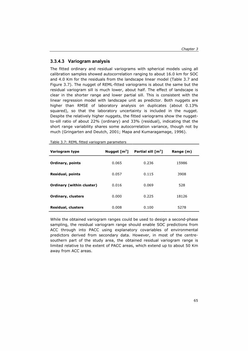
Chapter 3
3.3.4.3 Variogram analysis The fitted ordinary and residual variograms with spherical models using all calibration samples showed autocorrelation ranging to about 16.0 km for SOC and 4.0 Km for the residuals from the landscape linear model (Table 3.7 and Figure 3.7). The nugget of REML-fitted variograms is about the same but the residual variogram sill is much lower, about half. The effect of landscape is clear in the shorter range and lower partial sill. This is consistent with the linear regression model with landscape unit as predictor. Both nuggets are higher than RMSE of laboratory analysis on duplicates (about 0.13% squared), so that the laboratory uncertainty is included in the nugget. Despite the relatively higher nuggets, the fitted variograms show the nugget-to-sill ratio of about 22% (ordinary) and 33% (residual), indicating that the short range variability shares some autocorrelation variance, though not by much (Gringarten and Deutch, 2001; Mapa and Kumaragamage, 1996). Table 3.7: REML fitted variogram parameters
Variogram type Nugget [m2] Partial sill [m2] Range (m)
Ordinary, points 0.065 0.236 15986
Residual, points 0.057 0.115 3908
Ordinary (within cluster) 0.016 0.069 528
Ordinary, clusters 0.000 0.225 18126
Residual, clusters 0.008 0.100 5278
While the obtained variogram ranges could be used to design a second-phase sampling, the residual variogram range should enable SOC predictions from ACC through into PACC using explanatory covariables of environmental predictors derived from secondary data. However, in most of the centre-southern part of the study area, the obtained residual variogram range is limited relative to the extent of PACC areas, which extend up to about 50 Km away from ACC areas.
65

A DSM methodology for poorly accessible area
Figure 3.7: Ordinary and residual (landscape as covariable) variograms, all calibration points.
3.3.4.4 Within-cluster SOC spatial autocorrelation The experimental variograms along with a fitted pentaspherical variogram model for within-cluster spatial autocorrelation (up to 720 m) are shown in Figure 3.8. It reveals good spatial structure, with spatial dependence to about 500 m. The spatial dependence at short range was strong: nugget variance was fit to zero, but then raised to the known uncertainty of the laboratory analysis. The originally-modelled zero nugget shows the effect of composite sampling on a 90 m support. Thus most differences in SOC concentration are explained by local factors at scales between cluster range (720 m) and bulk sample range (90m). The linear model predicting SOC by sampling clusters (R2 = 0.71) has a residual mean square of 0.073%. This is the variance not explained by the clusters and should correspond to the sill of the within-station variograms, which were estimated at about 0.06 (% SOC)2. This also means that the nugget found in the long-range variogram represents a support of at least a cluster and that the clusters can be represented by their ordinary (unweighted) averages. Therefore spatial models as well as the remainder of the analyses were based on cluster averages. The averaging generally increased the proportion of SOC explained by the different explanatory variables (see Table 3.6).
66

Chapter 3
Figure 8: Ordinary Kriging experimental variogram of SOC up to a cut-off of cluster length (720 m), based on all calibration points.
3.3.4.5 Variogram analysis *clusters) Experimental variograms based on calibration cluster averages were difficult to model, due to the low number of point-pairs in each bin. Starting from the parameters of the fitted variograms based on all calibration points, spherical models were fitted (Figure 3.9, Table 3.7), resulting in slightly longer ranges, much lower structural sills and effectively zero nugget. These are all consistent with the averaging effect. The REML fit did not improve the variogram due to the high variance at smaller lag, pulling the REML variogram fit up and introducing an unrealistic nugget. Therefore the WLS fit was retained for mapping. The obtained variogram ranges increased by about 12% (ordinary) and 26% (residual), which potentially improves the ability for predictions in PACC from the ACC areas. This is despite the reduction in the partial sill. Cluster averaging will also be economical in future sampling as the within cluster variation will be ignored.
67

A DSM methodology for poorly accessible area
Figure 3.9: WLS and REML fitted ordinary (left) and REML fitted residual (right) variograms drawn based on calibration clusters (accessible areas).
3.3.5 Application of the model in accessible area SOC was predicted across ACC areas from the calibration observations, by applying the selected OK, KED and LM spatial models. Internal prediction quality was assessed by kriging prediction standard deviation (Goovaerts, 1999; McBratney et al., 2000). Since the within-cluster analysis showed that SOC in a cluster could be represented by the cluster average, prediction was performed by punctual kriging over 1x1 km grid as a support area, assuming that the average of a 1x1 km cell would to be similar to that of the 720x720 m support area for which spatial structure had a little longer than half the cluster length. The kriging prediction variance is thus realistic: “punctual” in this case means on a cluster-size support. The summary statistics of OK prediction (Table 3.8) shows OK with narrower range (1.27%) and the KED with the wider range (1.97%) and LM in between (1.44%). The same is observed for the mean SOC predictions by the three models. The OK prediction map clearly shows the effect of low sampling density. Areas further away from sampling locations are predicted as a spatially-weighted average (0.93%) as there is no information on spatial variation structure. Predictions by KED much resemble the landscape map (Figure 3.10).
68

Chapter 3
Table 3.8: Summary statistics of SOC (%) spatial prediction, Kriging prediction standard deviation (Kriging SD) and model independent validation.
model Prediction KPSD Independent
validation
Min Median Mean Max Mean IQR Mean RMSE Bias
OK_ACC 0.42 0.90 0.91 1.69 0.40 0.08 -0.03 0.50 -0.02
OK_PACC 0.46 0.90 0.89 1.68 0.44 0.04 0.09 0.36 0.09
KED_ACC 0.35 1.01 1.22 2.32 0.37 0.03 -0.01 0.42 -0.01
KED_PACC 0.40 0.97 1.06 2.17 0.37 0.03 0.06 0.31 0.06
LM_ACC 0.46 0.93 0.87 1.90 0.05 0.02 -0.03 0.45 -0.03
LM_PACC 0.46 0.92 0.84 1.90 0.05 0.01 0.07 0.31 0.07
Kriging prediction standard deviation (KPSD) is lower (Table 3.8) for the LM and higher for OK, with KED (Figure 3.10) in between the two, all with low IQR, suggesting that kriging prediction SD is a rather precise measure. However, the mean KPSD is about half (OK), a third (KED) and 5% (LM) the median and as high as the minimum predicted SOC (OK, KED) but only about 11% (LM). This suggests prediction quality by internal measure is better for LM and poor for OK and KED.
Figure 3.10: SOC (%) prediction maps by KED using landscape as a covariable (left) and its kriging prediction standard deviation (right).
69

A DSM methodology for poorly accessible area
3.3.6 Model validation in accessible areas Two validation measures were used; (1) the leave-one-out cross-validation (LOOCV) (Goovaerts, 1999; McBratney et al., 2000) as an internal measure of model fitness and (2) true validation with an independent sample set. Since there is no cross-validation concept for the linear regression model, it was not performed for the landscape model. LOOCV RMSE for both OK and KED are low, about 0.02% and mean prediction residuals are about 0.00% which indicate the models are unbiased. However largest residuals (±0.70%, symmetrical) are a little higher than the minimum prediction by the models. OK IQR of residuals is twice that of KED (0.29%). Independent validation results (Table 3.8) show KED and LM performing similarly (RMSE about 0.43%) and better than OK. Neither method is satisfactory given the fact that RMSE is a substantial proportion (about half) of the median from the model predictions. All methods are also biased (under-predictions). True validation RMSE is about double LOOCV RMSE in both cases, which is consistent with expectations. True validation RMSE and mean kriging SD are almost identical, and therefore kriging standard SD is a reasonable estimate of the actual error. At this point a decision had to made whether the model was sufficiently accurate to proceed to the next step of the methodology. Given the generally low values of the target variable in the LNP (maximum 2.68%, median 0.87%, see Table 3.5, and the result that the validation RMSE is about half the median, surely the model is of limited utility. It does show some landscape differences and accounts for spatial structure near the observation points, but even at a 1x1 km block gives predictions that are only about twice as precise as taking the area-weighted average or median observed value over the whole area. Nonetheless, the method is applied for the remainder steps for illustration purpose. To put the obtained results in context, they are compared with other studies reported in the literature. Mueller and Pierce (2003) studied the effect of sampling scale on accuracy of SOC predictions of top 20 cm across an area of 12.5 ha in Michigan, USA, and showed that despite the finer grids followed and a wide SOC range (0.2-0.29%), the best RMSEP obtained was 0.28-0.30%, about 30% of the SOC observed mean. Robinson and Metternich (Robinson and Metternicht, 2006) compared the accuracy of OK, lognormal OK, IDW and splines for interpolation of soil proprieties in 60 ha, south west Australia. The best OK RMSEP was 1.43% and about 30% of the average observed OM and 35% of the mean predictions. Chai et al. (2008) compared the performance of empirical best linear unbiased predictor (E-BLUP) with REML with that of RK for prediction of SOM in the presence of different external drifts across an area of 933 km2 in China. The best RMSEP obtained was 0.38% (RK), which represented about 29% of mean observed data. Grimm et al. (2008) predicted the spatial distribution of SOC following the DSM approach in Panamá for different soil depths in a 1500 ha area. The best
70

Chapter 3
RMSEP obtained was 1.72% for the top 10 cm soil depth, corresponding to about 34% of the observed SOC data. The above results show that the proportion of RMSEP to mean predictions or mean observed SOC in present study is poor relative to other studies. Comparative studies closer to the study area or in Africa, in general, are few but show different results. For example Stoorvogel et al. (2009) used a classification tree approach combined with existing knowledge from literature and a small data set to map top soil SOC content for a data-poor environment in a 1030 km2 of the Senegalese peanut basin, with a RMSEP of about 0.17%, representing about 40% of the mean observed SOC. As another example, Mora-Vallejo et al. (2008) tested whether DSM is suited for exploratory or reconnaissance soil survey of SOC. Their results in a 13 500 km2 area in southeast Kenya show SOC RMSEP of about 0.2%, corresponding to about 25% of both the mean predictions by regression kriging and mean observed SOC data. While these results are consistent with those from elsewhere, Schloeder et al. (2001) found rather more accurate results when they compared different interpolation methods (OK, IDW and thin-plate with and without tensions) for organic matter (OM) prediction across a 70x20 km area in the Omo basin, south-west Ethiopia. The best MSE was 0.08%, i.e., RMSE=0.28%, for OK, which represented about 20% of the mean observed data. Regardless of the different results, all are better than the one found in present study.
3.3.7 Application of the model in poorly-accessible areas SOC was predicted here using the same models (OK, KED and LM) for the same support area, also for the same reasons as in the ACC area. The internal prediction quality by kriging prediction standard deviation (KPSD) was also assessed (Goovaerts, 1999; McBratney et al., 2000). The summary statistics of OK prediction (Table 3.8) shows OK with narrower range (1.22% SOC) and the KED with the wider range (1.77%) and LM in between (1.44%). The same is observed for the mean SOC predictions by the three models. The OK prediction map (Figure 3.10) clearly shows the effect of low sampling density. Areas further away from sampling locations are predicted as a spatially-weighted average (0.93%) as there is no information on the structure of spatial variation. KPSD is lower (Table 3.8) for the LM and higher for OK, with KED in between the two, all with low IQR, suggesting that Kriging prediction SD is a rather precise measure. However, the mean KPSD is a little less than half (OK, KED) and 5% (LM) the median and as high as the minimum predicted SOC (OK, KED) but only about 11% (LM). This suggests prediction quality by internal measure is better for LM and poor for OK and KED.
71

A DSM methodology for poorly accessible area
Examples of the predictions into PACC based on models built from the ACC area, as proposed here, are not available in the literature. However, the obtained prediction results are within the range of those obtained (and discussed) for ACC areas.
3.3.8 Model validation in poorly-accessible areas The true validation was performed with an independent sample set as planned. Validation results (Table 3.8) show, surprisingly, all models with RMSEP lower than the one for ACC areas. Further KED and LM performed similarly (RMSEP about 0.31% SOC) and better than OK. However, all models performed poorly, given the fact that RMSEP are about 4/10 of the SOC prediction median, so effective mapping is not possible with the present sampling density. All models were also biased (under-prediction); with LM similar to KED and both a little better than OK. Mean KPSD was a little higher that validation RMSE (OK and KED) so KPSD is a reasonable estimate of actual error. Similar to predictions, validation results both the RMSEP (true validation) and KPSD (with exception to LM) found in the present study are about the minimum predictions and as high as double the mean predictions, which confirms obtained poor results in present study.
3.3.9 Relative performance of prediction model in PACC areas
When comparing validation RMSE between ACC and PACC, the three models performed better in PACC than in ACC areas by about 28% (OK) and 26% (KED) and 31% (LM). This is likely due to the different test set sizes (larger for the PACC). Thus the extrapolation into non-sampled PACC areas seems justified for KED, although predictions are largely determined by landscape away from sampling points in accessible area. LM performed relatively best and does not suffer from the requirement of spatial autocorrelation for interpolation into PACC areas. Despite poor predictions by both models, the methodology is promising because predictions into PACC areas are close to predictions made in ACC areas. The poor model predictions result from cumulative error effects brought about along the different steps, namely laboratory analysis, PLSR calibration, model building, and spatial predictions. The weak SOC variation explained by most of the explanatory variable here selected may also have contributed to the poor model predictions, although many authors have demonstrated the role of secondary data to improve prediction of SOC (Mueller and Pierce, 2003; Simbahan et al., 2006). Nevertheless, one of the strong points of obtained results lies on the spatial models’ range, which
72

Chapter 3
allows interpolation into PACC (about 5 Km KED and 18 Km for OK). Despite a longer range for OK, the low sampling density is a limiting factor as information on spatial structure is absent in the PACC. By contrast, KED allows mapping based on the covariable but the range of spatial structure is rather limited. LM can take over beyond the OK and KED range, into the PACC areas. The spatial models building was in this case made possible based on the integrated soil-forming factor (landscape) and the clusters, which explained most SOC variation. The OK results could be used to aid future sampling to improve prediction since the within cluster spatial structure is rather weak and could be bulked. Therefore future sampling could be based on the obtained structural range.
3.4 Conclusions The chosen test case turned out to be a difficult one. The range of SOC concentrations was narrow, weakly-dependent on covariables, and exhibited most of its spatial structure within the support of a cluster. It is concluded that SOC concentration in the study area varies mostly by local factors, probably current and past vegetation and animal activity (including termites), not captured by any covariable. The proposed method did work as planned in the sense that the models did as well in poorly-accessible as in accessible areas. The use of a previous integrative survey (Stalmans et al., 2004) was quite helpful in this case and was able to substitute for a large number of coverages. Such a survey substitutes for multiple factors in the scorpan-SPPfe framework. Despite the somewhat disappointing performance in this test case, the proposed methodology as such was appropriate, certainly as the first stage in a survey in areas with difficult access. At this point the spatial structure and relation of target variable with covariables are known, and there is evidence that the model structure in poorly-accessible areas is likely to be similar to that in accessible areas. Thus if not satisfied with the predictions mostly as landscape spatial averages, a sampling campaign can be planned by optimizing the KED variance to a realistic target (set here by the PLSR precision) as proposed by Brus and Heuvelink (2007). Certainly, in this case, is better to sample on a 1 km support and not try to map variation in smaller areas. All this could support preparation for the most efficient approach possible in the difficult circumstances of a survey in poorly-accessible areas.
73

A DSM methodology for poorly accessible area
74

Chapter 4 Building a NIR spectral library for the LNP3
3 This chapter is based on: Cambule, A.H., Rossiter, D.G., Stoorvogel, J.J., Smaling, E.M.A., 2012. Building a near infrared spectral library for soil organic carbon estimation in the Limpopo National Park, Mozambique. Geoderma 183-184, 41-48.
75
Building a NIR spectral library for the LNP
Abstract Soil organic carbon (SOC) is a key soil property and particularly important for ecosystem functioning and the sustainable management of agricultural systems. Conventional laboratory analyses for the determination of SOC are expensive and slow. Laboratory spectroscopy in combination with chemometrics is claimed to be a rapid, cost-effective and non-destructive method for measuring SOC. The present study was carried out in Limpopo National Park (LNP) in Mozambique, a data- and access-limited area, with no previous soil spectral library. The question was whether a useful calibration model could be built with a limited number of samples. Across the major landscape units of the LNP, 129 composite topsoil samples were collected and analyzed for SOC, pH and particle sizes of the fine earth fraction. Samples were also scanned in a near-infrared (NIR) spectrometer. Partial least square regression (PLSR) was used on 1037 bands in the wavelength range 1.25 – 2.5 µm to relate the spectra and SOC concentration. Several models were built and compared by cross-validation. The best model was on a filtered first derivative of the multiplicative scatter corrected (MSC) spectra. It explained 83% of SOC variation and had a root mean square error of prediction (RMSEP) of 0.32% SOC, about 2.5 times the laboratory RMSE from duplicate samples (0.13% SOC). This uncertainty is a substantial proportion of the typical SOC concentrations in LNP landscapes (0.45 – 2.00%). The model was slightly improved (RMSEP 0.28% SOC) by adding clay percentage as a co-variable. All models had poorer performance at SOC concentrations above 2.0%, indicating a saturation effect. Despite the limitations of sample size and no pre-existing library, a locally-useful, although somewhat imprecise, calibration model could be built. This model is suitable for estimating SOC in further mapping exercises in the LNP.
76

Chapter 4
4.1 Introduction The increasing need to manage land sustainably has triggered the debate on soil quality, its definition and the indicators best reflecting it (Arshad and Martin, 2002). Some researchers have developed indicators based on selected specific combinations of soil characteristics to characterize soil quality (Yemefack et al., 2006) but still there is no consensus on how the indicators should be interpreted (Bouma, 2002). However, all indicators related to soil quality include soil organic carbon (SOC) as one of the most important properties (Arshad and Martin, 2002). Shukla et al. (2006) states that if only one soil attribute were to be used for monitoring soil quality changes, it should be SOC. The widely-used soil fertility-crop production model QUEFTS uses SOC, or total nitrogen as a proxy (assuming a stable C/N ratio), as the major yield-explaining variable (Janssen et al., 1990; Liu et al., 2006; Pathak et al., 2003; Smaling and Janssen, 1993). This comes as no surprise in strongly weathered tropical soils that largely rely on the organic fraction for their inherent soil fertility. SOC is also recognized as the best entry point for land degradation assessment (Gisladottir and Stocking, 2005). Assessment of SOC over larger areas by field sampling and conventional laboratory analysis is expensive and slow. Laboratory spectroscopy is widely-applied in chemometrics (Geladi and Kowalski, 1986) and recently also to soil characterization (Brown et al., 2006; Shepherd and Walsh, 2002). It offers rapid and about 50% cheaper soil analysis (Cécillon et al., 2009a), and, as an added benefit it is non-destructive, so samples can be analysed repeatedly. The most common form of spectroscopy for SOC determination is visible and near-infrared reflectance (VNIR, 0.4 – 3.0 µm) and - mid-infrared (MIR, -3.0 –30 µm) (Clark, 1999). Other authors indicate different spectral ranges for the same regions, e.g. Vis-NIR-SWIR to be 0.4-2.5 µm (Ben-Dor, 2002; Shepherd and Walsh, 2002). SOC produces a spectral signature, defined by the reflectance or absorbance of electromagnetic radiation as a function of wavelength. In the case of SOC, as with the absolute majority of absorbants, combination of bands and overtones of the fundamental spectral features are detected in the NIR regions (Shepherd and Walsh, 2002). Direct quantitative prediction from spectra is almost impossible because soil constituents interact in a complex way to produce a given spectrum. Therefore, quantification of the property of interest is done with multivariate statistical models (Cécillon et al., 2009b). Viscarra Rossel et al. (2006) demonstrated the potential of reflectance spectroscopy along with the chemometric methods applied to develop these multivariate statistical models to predict soil properties. Partial least-squares regression (PLSR) and principal components regression (PCR) were the multivariate methods most applied for SOC determination, while sample size varied from 68 to 674,
77

Building a NIR spectral library for the LNP
resulting in a calibration R2 of 0.86 - 0.96. However, only three of the reported 14 studies on SOC had a sample size bellow 150. Shepherd and Walsh (2002) indicate that as the sample size decreases, the predictive performance decreases gradually at large sample sizes but rapidly as sample size decreased between about 100 to 200 samples to a R2 < 0.7 and even below 0.5 for sample sizes smaller than 100, implying more relative variation in the dataset. Despite the reported problems with small sample sizes, there are many situations where it is impractical to obtain large sample sizes. Typical limitations are financial, access, and logistical (limited conventional laboratory facilities, limited access to spectrometers, limited trained technicians). Studies with such limitations have to make the best out of the limited data that can be collected and analyzed. However, local calibrations with small sample sizes may be possible if soil variation is limited within a specific study area (Brown, 2007). Small sample sizes in a particular study are not a problem if there is a calibrated spectral library which includes soils similar to those collected in the new study (Shepherd and Walsh, 2002), but for many areas of the world, and for many soil types, such libraries do not exist. Thus, the objective of this study was to test whether a locally-developed calibration model for SOC based on a limited number of samples can be developed within the context of a project with limited resources, in an area of limited access, and where no soil spectral library exists.
4.2 Materials and methods
4.2.1 Soil samples and spectral acquisition Soil samples are the same as those used for DSM (chapter 3). In the soil laboratory, samples were air-dried, gently crushed and passed through a 2 mm mesh sieve to collect the fine earth fraction. Samples were put in petri dishes and then scanned in a Bruker FR-NIR MultiPurpose Analyser (MPA), (Bruker optic GmbH, Ettlingen, Germany) located in the Instituto de Investigação Agronómica de Moçambique (IIAM), Maputo. This instrument has built-in validation to perform instrument internal (operational and performance) quantification tests, and its spectrum is calibrated before each scan to an internal gold reference. Spectra were recorded from 0.8 to 2.6 µm
at a spectral resolution of 1250 µm, with zero-filling factor of 2, resulting in an effective bandwidth of 3.86µm. Each spectrum is an average of 64 scans. Spectra were further reduced to the range 1.25 – 2.5 µm as these bands contain most of relevant information.
78
Chapter 4
4.2.2 Selection of soil samples for reference analysis To form a subset of samples for reference analysis, a total of 129 samples were selected from both DSM calibration (104) and validation (25) sample sets as described in previous Section. The samples represent one third and one fourth of DSM calibration and validation sets (chapter 3), respectively. These proportions are commonly used in laboratory spectroscopy (Brown et al., 2005; Grinand et al., 2008). Reference samples from DSM calibration were used for model calibration (about four fifth) and those from DSM validation, used for model validation (about one fifth); note these are here referred to as “model” calibration and validation, as opposed to the “DSM” calibration and validation sets from field sampling. To select a representative set covering the range of spectra and SOC contents, the spectra were compressed using principal component analysis (PCA), to summarize the data and examine its structure. The PCA scores were grouped by computing a K-means clustering in the Unscrambler 9.7 program (CAMO Software AS, Nedre Vollgate, Oslo, Norway). The number of groups was determined iteratively to minimize the sum of distances (SOD). Samples were randomly chosen from the different groups as suggested by Martens and Naes (1986) in order to enhance sample set diversity (Stenberg et al., 1995). Samples were then drawn from these groups, excluding any that met any of the following three conditions: (1) high residuals and low leverage, (2) both high residual and leverages or (3) high leverages and away from the PCA model trend, were considered outliers and not considered for laboratory analysis (Esbensen, 1994). Outliers as thus defined were automatically flagged based on the default threshold values in Unscrambler 9.7.
4.2.3 Laboratory analysis The selected samples were analyzed in the soils laboratory of Eduardo Mondlane University, Maputo, for SOC and possible co-variable predictors soil pH and particle size fractions, following standard ISRIC methods for soil laboratory analysis (van Reeuwijk, 2002). SOC was determined by the Walkley-Black method. Soil pH was measured potentiometrically in a supernatant suspension of 1:2.5 soil:liquid mixture (two determinations: in distilled water and 1 M KCl solution). Particle-size separates of the fine earth (<2 mm) fraction were determined after cementing agents were first removed by means of hydrogen peroxide, calgon and calcium chloride solution. The sand fraction (2 mm - 50µm) was washed onto a 50µm sieve, after which silt (50µm - 2µm) and clay (<2µm) fractions were determined by hydrometer method. Twenty randomly-selected samples were analyzed in duplicate for quality control and to quantify laboratory precision.
79

Building a NIR spectral library for the LNP
4.2.4 Calibration and validation Mathematical and statistical procedures were carried out in the R environment for statistical computing (Ihaka and Gentleman, 1996), Unscrambler (CAMO Software AS, Nedre Vollgate, Oslo, Norway), and ParLes (Viscarra-Rossel, 2008). The “pls” package was used within R for multivariate calibration (Mevik and Wehrens, 2007). PLSR was used to develop models based on spectra and reference laboratory data of the 129 selected soil samples. Models were evaluated in two ways: (1) “leave-one-out” cross-validation on models developed with all 129 samples and (2) true validation by splitting the sampling set into spectral calibration (104 samples) and validation (25 samples) sets. The former was used to search for the best pre-processing of the raw spectra and the latter to obtain realistic estimates of prediction accuracy. Models were attempted with the original spectra, multiplicative scatter corrected (MSC) spectra, first derivatives of these; and all of these also after applying a Savitsky-Golay filter (2nd order polynomial covering 11 adjacent bands). MSC was applied since the original spectra showed additive effects which could result from differential scattering in the granular sample. The derivative transformation minimizes the effect of variation in sample grinding and optical set-up (Shepherd and Walsh, 2002). Transformations of the laboratory measurements were also attempted but did not improve results and therefore are not reported. Model calibration accuracy was evaluated by means of the root-mean squared error of calibration (RMSE) of the cross-validation predictions, and R2 (proportion of variation explained) of the SOC vector. Because the resulting model was intended to be used to map SOC across the LNP, there was no option of rejecting any observations as outliers. Prediction accuracy was assessed by the ratio of standard deviation (SD) to RMSE of cross-validation and by the multiple R2 (Chang et al., 2001; Waiser et al., 2007). In an attempt to improve the predictive performance of the best PLSR model and following a suggestion by (Fearn, 2010), the proportion of clay in the fine earth - a commonly used covariate for SOC spatial interpolation (McGrath and Zhang, 2003; Mutuo et al., 2006), - was added to the spectra information as a supplementary “band”, and a new PLSR model built. Clay proportion may be helpful for PLSR modelling in cases where a collection of samples and its laboratory analysis results for clay (but not SOC) from past surveys is kept. For new surveys the laboratory costs of determinating clay and SOC are comparable, so these models are not relevant. Clay variance was inflated 86 times to match the true dimensionality of spectra predictors so that it could be properly weighted, on the basis that previous PLSR model
80

Chapter 4
did explain most of SOC variation with about 12 factors (as shown in the results, below); 12 x 86 = 1037, the approximate number of spectral bands.
4.3 Results and discussion
4.3.1 Sample selection for reference analysis Figure 4.1 shows the sample selection procedure for reference analysis from the DSM validation set. The first two principal components explained 98% (91 + 7%) of spectra variation; the SOD was achieved for 6 clusters. The influence plot was used to identify outliers. The same procedure was followed for the DSM calibration set, where the first two PC’s explained 98% (95 + 3%) of spectra variation and the minimum SOD was achieved for 12 clusters. As per the sampling plan 25% (=25) of DSM validation and 1/3 (=104) of the DSM calibration sets were selected for reference analysis. Since the number of PCA score groups (intended to represent spectra variability) was small, more than one sample was selected from most of them. The small number of groups indicates the fairly homogeneous nature of the sample sets. This procedure has also been followed by other workers (Viscarra-Rossel and Behrens, 2010) to select samples based on spectral variability. Whereas PCA score grouping enhances spectral diversity, it may also enhance the spatial autocorrelation between the selected samples due to possible coincidence of PCA score groups with the field sample clusters. This raises the possibility of false precision (Brown et al., 2005). However, RPD (Figure 4.5) suggests that this effect is minimal in present case.
Figure 4.1: Score plot of the first two principal components principal of spectra from DSM calibration set symbolized by their cluster (left) and sample influence plot (right) used to select samples for reference laboratory analysis.
4.3.2 Soil properties The summary statistics of laboratory analysis (Table 4.1, Figure 4.2) show a fairly wide range for SOC in this semi-arid environment, from below the detection limit to moderate values (2.7%), thus providing a good range for model calibration. Soils range from quite acid to alkaline, with a somewhat left-skewed distribution emphasizing the alkaline range. Most are coarse-textured. The empirical distributions of SOC, clay and silt appear positively
81

Building a NIR spectral library for the LNP
skewed while that of the sand fraction is negatively skewed. Parametric correlations between duplicates were all linear and generally very good. Laboratory duplicate RMSE (on the expected 1:1 line) were low, indicating good analytical precision. The moderate precision for particle sizes matches the expected precision of the hydrometer method. These RMSE set an upper limit on the precision of any calibration. Bivariate correlations between soil properties showed positive correlations between SOC and pHH20 (0.50), pHKCl (0.49), clay (0.56) and a negative correlation between SOC sand (-0.65), all significant at 0.01 level. These results are expected: finer-textured soils retain moisture longer, and neutral to alkaline soils generally support more soil microorganisms and more vigorous vegetation (hence more leaf litter); both of these situations are conducive to higher levels of SOC. Table 4.1: Summary statistics for 129 soil samples set submitted for reference laboratory analysis. Included is the correlation coefficient (r) of duplicate samples as well as the RMSE from 1:1 line. Summary statistics (N = 129)
Soil property pH water pH KCl SOC (%) Clay (%) Silt (%) Sand (%)
Minimum 3.7 3.4 0.0 5.3 0.0 2.2 1st quartile 5.7 5.3 0.4 8.7 1.8 74.4 Median 6.7 6.2 0.7 13.9 4.6 81.3 Mean 6.5 6.1 0.9 14.4 7.4 78.3 3rd quartile 7.6 7.3 1.2 17.3 8.7 88.8 Maximum 9.0 8.1 2.7 47.3 50.5 93.5 SD 1.1 1.2 0.6 7.1 8.5 14.4 r (duplicates, n =20) 0.96 0.99 0.97 0.89 0.93 0.98 RMSE (from 1:1 line) 0.32 0.17 0.13 2.6 3.2 2.9
82

Chapter 4
Figure 4.2: Distribution of soil properties in laboratory samples; bars = histogram, dashed line = density and fine dashed line =normal fit), Soil fractions units in percentages. Rug marks along the x-axis show individual sample location.
4.3.3 Laboratory SOC vs Landscape units Mean SOC per landscape units is highest in CMR (2.00%), decreasing through PS (1.15%), MSC (0.95%), SAF (0.91%), LLF (0.60%) and NS
83

Building a NIR spectral library for the LNP
(0.45%). Note that the laboratory RMSE for SOC (0.13%) is a significant proportion of the low-SOC landscape units. Duncan’s multiple-range test shows that CMR is clearly separated from all other landscape units, NS and LLF are grouped at the lower end and cannot be separated from the grouping of MSC and SAF. This group cannot also be statistically separated from PS, due to the wide ranges of SOC for MSC, SAF and NS (Figure 4.3). ANOVA shows that landscapes explain about 24% of the total SOC variation. Thus SOC is rather similar over most of the landscape, which should reduce prediction errors due to the small sample size. Separate analysis per landscape is in any case not possible because of the limited number of samples; this result shows that such an analysis would be unlikely to result in different models.
Figure 4.3: Box-plots and Duncan’s multiple range test (alfa = 0.05 and Df=117) for the SOC per landscape unit.
4.3.4 Spectral features The raw spectra (Figure 4.4) generally showed the typical pattern of soil spectra, with three major absorption features around 1.37-1.46, 1.86-2.06 and 2.14-2.26 µm. The first absorption region (near 1.4 µm) is the first overtone of OH stretches (moisture adsorbed to the clay surfaces) and near 1.9 µm it is the combination of OH stretches and H-O-H bend in water molecules trapped in the crystal lattice (not present in for example well developed dried Kaolinites). Near 2.2 µm it is OH-metal bend and OH stretches combinations where the metals can be AL or Fe or Mg substituting Si (Fe and Mg closer to 2.3 µm) Clark et al. (1990). In addition, a number of spectra showed two noisy (or fluctuating) reflection regions around 1.34-1.39
84

Chapter 4
and 1.79-1.92 µm. These ranges overlap with the first two absorption features. These raw spectra are similar to those found by other authors, e.g. Ben-Dor et al. (1999) and Ben-Dor and Banin (1995). The SOC component normally affects the overall positioning and shape of the spectrum (Shepherd and Walsh, 2007).
Figure 4.4: Spectra of the soil samples showing three major absorption features, related to OH groups in both absorbed water (≈ 1.4 and 1.9 µm) and the crystal lattice water (≈ 2.2 µm), (Ben-Dor and Banin, 1995)
4.3.5 Prediction of SOC from NIR spectra Since there is no a priori way to determine which spectra pre-processing methods result in the best predictive model (Ben-Dor and Banin, 1995), a number of spectra pre-processing methods were compared (Section 4.2.4). Pre-processed spectra showed peaks at around the same wavelength ranges as the raw spectra, regardless of pre-processing method. The best PLSR model (Figure 4.5), MSC smoothed and 1st derivative) for the prediction of SOC in the LNP was obtained with nine factors with a RMSEP of about 2.5 times that obtained from laboratory analysis on duplicate samples . The model also explained 99.5% of spectra variance. The median cross-validation residual was –0.0035%, inter-quartile range (IQR) –0.015 to +0.013%, but there were some very poorly-modelled points, at the extremes –1.25 and +1.75% SOC. The loadings of the first two model factors explained 95.1% of spectral variation; The other pre-processing methods (Figure 4.5) resulted in PLSR models with RMSE slightly higher (0.36 to 0.32% SOC) and therefore lower SOC explained variation. In addition about half of these models suffered from non-linearity effects expressed in the form of “banana-like” trends, causing underprediction for the extreme values. The 5% absolute extreme values of best model’s regression coefficients (Figure 4.7) show regions that were important for SOC predictions. These regions are in
85
Building a NIR spectral library for the LNP
good agreement with those where assigned SOC spectral features are located. However, these interpretations should be considered with caution given the fact that is made on the base of pre-processed spectra (MSC smoothed 1st derivative spectra), which may not be as useful as if the analysis would have been carried out on the base of raw spectra, as peaks in raw spectra are represented by. In pre-processed following derivatives, peaks will occur at maximum slopes of the original spectra and the original peaks will occur as crossing the zero line. Thus, in the derived spectrum each original peak will be represented by one positive and one negative peak. The MSC minimized the amplification and offset effects of light scattering in the raw spectra, which resulted in PLSR calibration improvement. Shepherd and Walsh (2002) preferred the first derivative pre-processing technique to MSC, as the latter did not improve multivariate adaptive regression tree (MART) calibration. The first derivative is the most commonly applied transformation to minimize variation among samples caused by variation in grinding and optical set-up (Stenberg et al., 2010). MSC is not preferred by many authors because it is difficult to locate an adequate spectral range to apply, raising the risk of affecting relevant spectral features for the component of interest (Esbensen, 1994). Despite the acceptable model reliability, the proportion of RMSEP to the mean SOC of sample set is substantial, about 36%. Literature shows this proportion varies considerably. For example Fidêncio et al. (2002) determined SOM by radial basis function networks and NIR spectroscopy and found a proportion of RMSEP to mean SOC of between 9 and 108%, Brown et al. (2006) obtained a proportion around 265%, and Terhoeven-Urselmans et al. (2010) of about 190%. Better proportions were obtained by Shepherd and Walsh (2002), about 18%, Fystro (2002) about 20%, and Wetterlind et al. (2008) about 8%. Most of the high proportions are from studies covering large areas as does the present study, which suggests room for further improvement by spiking (Guerrero et al., 2010), i.e., inclusion of a few local samples. The obtained results are between the local and large-area studies, hence being here characterized as “regional”.
86

Chapter 4
Figure 4.5: SOC PLSR prediction models derived as a function of spectra pre-processing method; (a) –(h) which included a combination of raw (original)/smoothed spectra, multiplicative scatter correction (MSC), standard normal variate (SNV), and 1st derivative. (i) shows SOC PLSR model derived from inclusion of clay covariable in the predictor set. Although the best model found in the present study fitted well the 1:1 validation line, all eight observations with SOC concentrations above 2.0% were under-predicted. In addition there were three observations with moderate SOC concentrations but large negative residuals (over-predictions). The cause for these poor predictions was investigated by plotting the SOC against pH and clay proportion. Clay did not give an obvious explanation as it spanned a wide range for the poorly-predicted samples. The pH was in the range 6 – 7.5 for the underpredicted samples and around 8 for overpredicted ones. The pH range 7.8 – 8.4 is often indicative of carbonate presence (Schumacher, 2002). However, no effervescence was observed after addition
87

Building a NIR spectral library for the LNP
of HCl 10% to the samples. There was also no apparent relation between landscape units and poor predictions (Figure 4.6).
Figure 4.6: The best PLSR prediction model showing the samples symbolized by the landscape unit (Stalmans et al., 2004) from where they were collected. A scatterplot of SOC against clay or clay + silt revealed a fairly strong relation at lower values, which degraded above about 18% clay or 25% clay + silt. This disagrees with results reported by Stenberg (2010) , who found out that prediction of SOM could be substantially improved by removing the sandiest soils. The wavelengths contributing most for the best model in the present study are near 1.4, 1.9 and 2.2 µm, which correspond to OH groups of soil moisture (first two) to the crystal lattice in soil clay minerals (last) (Ben-Dor and Banin, 1995) (Figure 4.7). Although the latter do overlap with assigned wavelength for the determination of the alkaline-earth carbonates, calcite and dolomite by near infrared spectroscopy, it was not possible to identify them, possibly because carbonate content was not detected (far below the 10% weight basis threshold) and that samples were not pre-heated to 600 ºC for 8 h in order to remove the strong absorption features of OH groups both in the organic matter and clay minerals, to enhance CO3 features (Ben-Dor and Banin, 1990). Ben-Dor and Banin (1995) identified the 1.4 and 1.9 μm bands as important for prediction of soil organic matter, while they are at the same time
88

Chapter 4
characteristic for OH and water molecules. This confirms the difficulty in identifying with confidence the spectral ranges characteristics for different compounds (Ben-Dor et al., 1999; Clark, 1999; Brown at al., 2006; Stenberg, 2010)
Figure 4.7: The 5% extreme values of PLSR coefficients (2.5% positive and 2.5% negative) of best model, showing the most contributing wavelengths ranges for model predictions. PLSR is a data compression method that summarizes most of variables’ variance in a few factors and by so doing helps to reveal hidden patterns in the data (Esbensen, 1994). The analysis was performed here on the pre-processed spectra to help explain whether landscape units may have influence on the model prediction ability and therefore explain its poor performance for some of the samples. The score plot of the first three PLSR components (factors) did not reveal landscape-related pattern, except for the LLF (Limpopo Levubu Floodplains) landscape unit which did follow a specific pattern, but samples collected in this unit were not a problem for the prediction model. Thus there are groups of similar samples but these did not separate under- from over-predictions. The normal probability plot of SOC residuals suggests that the PLSR model may still have some non-linearity, as the sample residuals at both ends slightly deviated from the tails of the normal distribution. All the under-predicted samples are located at the upper end of this plot while, surprisingly, the over-predicted ones do fall within the linear range of the plot.
89

Building a NIR spectral library for the LNP
4.3.6 Calibration subset models The best model form (smoothed first derivative of MSC-corrected spectra) was fit to the 104-observation DSM calibration subsample. A nine-component PLSR model had an internal cross-validation RMSEP of 0.323% SOC, just a little worse than the model from the full set, 0.315%. Predictions from this model for the 25-observation spectral validation had errors from -0.50 to +0.65%SOC, with a median of -0.10% and inter-quartile range (IQR) from -0.22 to +0.27%; compared to cross-validation errors these are much lower extremes but wider IQR. The true validation RMSEP was 0.331%, just a bit higher than the full-set cross-validation RMSEP of 0.315%. This shows that (1) cross-validation gives a realistic estimate of the true validation error, (2) the model built from DSM calibration spectra only is a little less accurate than that built from all spectra; (3) the 104/25 split fairly reflects model performance; (4) the DSM calibration and validation samples have similar characteristics.
4.3.7 Prediction of SOC from NIR spectra and Clay The PLSR model based on the NIR + clay (Figure 6), following same spectra pre-treatment, shows some improvement compared to that based on the NIR spectra only. The best model now contained only seven factors (Figure 6 (i)), explaining 100.0% of clay + spectra and 84% of SOC variances, with a RMSEP of 0.28% SOC, about 0.04% better than the model without the covariate) and slightly above twice as much as that obtained for laboratory analysis on duplicate samples. Almost all clay + spectra variance is explained by the first factor, while this component explains about 32% of SOC. The remaining 52% of explained variance attained at the seventh factor of the model is generated by a cumulative < 1% clay + spectra variance. This result is not surprising, given the generally good relation between clay and SOC in this sample set, and the strong diagnostic features in clay spectra. This result agrees with that of Brown et al. (2006), who showed that the inclusion of sand fraction and soil pH as auxiliary predictors improved calibrations.
4.4 Conclusions Using only 129 samples combined from the different landscape units of the LNP resulted in a fairly stable, effective NIR PLSR calibration model for SOC prediction in the target area. The model predicted fairly well irrespective of landscape unit. However, model performance was limited at higher SOC concentrations. The stable and effective model here obtained from a limited number of samples shows that reasonable models can be built for areas of
90

Chapter 4
limited access, where a limited number of representative samples can be collected, as it is the case of LNP. The addition of a moderately-correlated covariable (here, clay concentration) in the set of predictors slightly improved the precision (RMSE). This is of interest in the case where there are stored samples where particle-size has been analysed in the lab; these samples may now be scanned and the developed predictive equations used to estimate SOC. Despite the improvement of model accuracy by inclusion of clay, errors are still a substantial proportion of mean prediction. This suggests that caution must be considered when using spectroscopy to estimate SOC for mapping or monitoring low-SOC landscapes. While the model has a potential for SOC prediction in regional and baseline studies, it can be improved further for detailed ecological and farm-level studies within the LNP or in similar nearby soil landscapes by recalibrating the model after adding a few “local” samples (spiking).
91

Building a NIR spectral library for the LNP
92

Chapter 5 SOC stocks in the LNP - Amount, spatial distribution and uncertainty4
4 This chapter is based on: Cambule, A.H., Rossiter, D.G., Stoorvogel, J.J., Smaling, E.M.A., (under review). Soil Organic Carbon stocks in the Limpopo National Park, Mozambique: amount, spatial distribution and uncertainty. Geoderma.
93

Building a NIR spectral library for the LNP
Abstract Many areas in sub-Saharan African are data-poor and poorly accessible. The estimation of Soil Organic Carbon (SOC) stocks in these areas will have to rely on the limited available secondary data coupled with restricted field sampling. The total SOC stock, its spatial variation and the causes of this variation was assessed in Limpopo National park (LNP), a data-poor and poorly accessible area in southwestern Mozambique. During a field survey, A-horizon thickness was measured and soil samples were taken for the determination of SOC concentrations. SOC concentrations were multiplied by soil bulk density and A-horizon thickness to estimate SOC stocks. Spatial distribution was assessed through: i) a measure-and-multiply approach to assess average SOC stocks by landscape unit, and ii) a soil-landscape model that used soil forming factors to interpolate SOC stocks from observations to a grid covering the area by Ordinary (OK) and Universal (UK) kriging. Predictions were validated by both independent and leave-one-out cross validations. The total SOC stock of the LNP was obtained by i) calculating an area-weighted average from the means of the landscape units and by ii) summing the cells of the interpolated grid. Uncertainty was evaluated by the mean standard error for the measure-and-multiply approach and by the mean kriging prediction standard deviation for the soil-landscape model approach. The reliability of the estimates of total stocks was assessed by the uncertainty of the input data and its effect on estimates. The mean SOC stock from all sample points is 1.59 kg m-2; landscape unit averages are 1.13 - 2.46 kg m-2. Covariables explained 45% (“soil”) and 17% (coordinates) of SOC stock variation. Predictions from spatial models averaged 1.65 kg m-2 and are within the ranges reported for similar soils in southern Africa. The validation Root Mean Square Error of Prediction (RMSEP) was about 30% of the mean predictions for both OK and UK. Uncertainty is high (coefficient of variation of about 40%) due to short-range spatial structure combined with sparse sampling. The range of total SOC stock of the 10 410 km-2 study area was estimated at 15 579 - 17 908 Gg. However, 90% confidence limits of the total stocks estimated are narrower (5 – 15%) for the measure-and-multiply model and wider (66 - 70%) for the soil-landscape model. The spatial distribution is rather homogenous, suggesting levels are mainly determined by regional climate.
94

Chapter 5
5.1 Introduction Soil organic carbon (SOC) drives natural soil fertility and is a common indicator of livelihoods and ecosystem functions. It has been a focus of attention in the context of both agricultural development and carbon sequestration. Under the various United Nations protocols, there is an increasing need for accurate estimates of SOC stocks at national and sub-national scale to aid policy makers in making land use and management decisions (Milne et al., 2007). Estimates of current SOC stocks and their spatial variation are the starting point for the estimation of the carbon sink capacity and SOC sequestration. The focus of the study determines the type of data required. In the case of climate change, estimates of total SOC stocks are important for mitigation purposes. However, when carbon payments are considered, the spatial distribution of stocks and their respective change become important (Antle et al., 2007). Techniques for estimating SOC stocks have been grouped into two categories (Mishra et al., 2010; Thompson and Kolka, 2005): (1) the measure-and-multiply approach and (2) the soil-landscape modeling approach. In the measure-and-multiply approach the study area is stratified. Point measurements per stratum are averaged and multiplied by the area of each stratum of maps that stratify (Guo et al., 2006; Tan et al., 2009; Thompson and Kolka, 2005). Soil survey maps and field observations are primary resources to estimate SOC stocks with the measure and multiply approach that has been applied from regional (Amichev and Galbraith, 2004; Batjes, 2008; Tan et al., 2004; Thompson and Kolka, 2005) to global (Batjes et al., 2007) scales. The approach has the advantage of being simple, though it is not exempt of several limitations like potentially high within-stratum SOC variability (Mishra et al., 2010; Thompson and Kolka, 2005). The soil landscape modeling approach analyzes the spatial variability of SOC stocks with respect to variations in environmental covariables such as topography, land use or climate (Mishra et al., 2010). A model is built based on the various environmental covariables covering the entire study area plus limited number of field observations of SOC stocks, and is used to make predictions over a grid across the study area (Gessler et al., 2000a; Thompson et al., 2001). These are then summed to an area total. Examples of use of this approach are many, e.g., Ungaro et al. (2010) and Ziadat (2005), though many have successfully been applied to small areas (< 100 ha) and using of digital elevation models as the covariate, e.g. Florinsky et al. (2002), Bhatti et al. (1991) and Gessler et al. (2000a). The soil-landscape approach may result in a lower estimation error at each prediction location, due to the use of complete spatial coverages of secondary information, i.e., the environmental covariables. The measure-and-multiply approach has the advantage of simplicity, although within-stratum variability
95

Building a NIR spectral library for the LNP
(heterogeneous strata) limits precision (Aubry and Debouzie, 2000; Mishra et al., 2010; Thompson and Kolka, 2005). Further, the soil-landscape approach produces a grid map of SOC stocks whereas the measure-and-multiply approach produces a chloropleth map with an average value per stratum. It is not clear a priori which method gives lower estimation errors for total stocks. In 2001, Mozambique declared an area known as “Coutada 16” (hunting zone) the LNP, which forms part of a trans-frontier park with South Africa and Zimbabwe. The LNP provides ecosystem services and supports the livelihoods of about 20 000 people living within its boundaries. The formation of LNP and the planned relocation of the communities within the park will result in major land use changes, both in terms of vegetation and wildlife (Ministerio do Turismo, 2003). These changes are expected to affect SOC stocks in and around the LNP, including in resettlement areas where SOC stocks are a major contributor to soil fertility. Any change cannot be assessed without a proper baseline, i.e. present-day stocks. Therefore, the aim of this study was to quantify the total SOC stock and its spatial variation in the Limpopo National Park, and the probable causes of any variation. Furthermore, to compare the various approaches to estimating SOC stocks.
5.2 Material and methods A summary of the methodology follows; later in the section each step is explained in detail. We assessed SOC stocks for sampling points, its variation across the LNP by landscape, and the total SOC stock. First SOC concentrations were converted to SOC stocks at the sampling points using the field measured A-horizon thickness and estimated soil bulk density. To estimate the SOC stocks distribution across the LNP, two approaches were followed: (a) the measure-and-multiply method where mean stocks are calculated per landscape unit, and (b) the soil-landscape approach where stocks are estimated over a grid using spatial models derived using auxiliary information and limited field sampling. Total stocks were calculated by summing up (a) the estimated stocks of the landscape units and (b) the estimates at each grid cell. In addition, total stocks were estimated based on calculated naïve and spatial means converted to LNP area size. The uncertainty of estimates of stocks’ spatial distribution was also assessed by calculating the standard error (SD of the mean) and kriging prediction standard deviation, respectively for the measure-and-multiply and soil-landscape approaches. Uncertainties of estimates of total stocks were obtained by calculating the standard error and mean kriging prediction standard deviation plus the 90% confidence interval. Finally the reliability of the estimates of total stocks was assessed by assessing the uncertainty of the input data and its effect on estimates of total stocks. The results from the various methods are then compared based on their width of confidence
96

Chapter 5
interval (Janssen and Heuberger, 1995; Smith et al., 1997; Wösten et al., 2001). Statistical analysis was performed in the R environment for statistical computing (R Development Core Team, 2006).
5.2.1 Assessing SOC stocks SOC stocks at the sampling points To assess SOC stocks at sampling points, the field-identified A-horizon was chosen as the sample volume because it is where most biological activities take place and therefore most of the soil carbon is stored (Gessler et al., 2000a). SOC concentrations obtained in chapter 3 (in Table 3.5) were converted into SOC stocks using the field measured A-horizon thickness and soil bulk density (BD), estimated as 1.44 ± 0.02 g.cm-3. This estimate is based on measurements (n = 14) by COBA Consultores (1982) around the confluence area between the Singuedzi and Elefant Rivers and Nhantumbo et al. (2009) on the sandy soils in the extensive NS landscape unit. This average was used instead of estimating BD at each point by a pedotransfer function (PTF) from the measured clay content and SOC concentration, because there is no calibrated PTF for the area and the use PTF developed elsewhere is not appropriate even under similar ecological conditions (Gijsman et al., 2002). The average BD used is consistent with ranges reported in the literature by EUROCONSULT (1989) for the sandy loam to sandy clay loam soil textural classes found in LNP (1.4 – 1.65 g.cm-3). The practice followed here is consistent with that of Williams et al. (2008) in the miombo woodlands of central Mozambique, who justified the use of a single value of BD (1.29 cm-3) because of the low variability of BD from 28 composite topsoil samples. Despite the similarity in soil textural classes, their study site is located in a much wetter climate than LNP study area (annual precipitation of about 700 mm vs. 450 mm) as depicted by the much richer miombo vegetation, so the soils with higher organic matter are expected to have lower BD. SOC stocks spatial distribution The measure-and-multiply approach In this approach the spatial distribution of SOC stocks across the LNP was interpreted to be a function of the sampling strata, i.e., the landscape map of Stalmans et al. (2004). In this approach an average of each landscape unit was calculated based SOC stocks data from sampling points. The averages were computed by a single-factor ANOVA (R function ‘lm’), followed by a pairwise means comparison with pooled standard deviation and the Holm correction for multiple comparisons (R function ‘pairwise.t.test’) to group and rank landscape units, thus showing the stocks spatial distribution across the LNP as a chloropleth map of single values (with uncertainty) per landscape unit.
97

Building a NIR spectral library for the LNP
The soil-landscape approach Here we interpreted the spatial distribution of SOC stocks across LNP as a function of soil-forming factors (McBratney et al., 2003). These were represented by explanatory variables derived from readily-available, full-coverage secondary information. Spatial models were developed to describe the variation in SOC stocks in relation to the soil-forming factors. These steps are now described in detail. (a) Soil-forming explanatory variables
The framework for digital soil mapping described by McBratney (2003) was followed. In the study area SOC stocks are expected to be related to a number of soil forming factors including rainfall, vegetation, topography, parent material, and soil conditions. Selected secondary data corresponding to these soil forming factors (Table 2) include the same five secondary data collected for DSM (chapter 3). First- and second-order trend surfaces, which are surrogates for regional change in soil-forming factors, were also considered.
(b) Selection of explanatory variables for spatial models
To select the explanatory variables for model building, their values at sampling points were first extracted through map overlay. The SOC stock at these points was linearly regressed on the continuous explanatory variables, and as a one-way or multiway linear partitioning of variance for the categorical variables, both using R function ‘lm’. Models were evaluated by ANOVA of the model compared to a null model, and by visual inspection of regression diagnostic plots (Fox, 1997). The highest adjusted goodness-of-fit of models with acceptable diagnostics was used to select explanatory covariables for model building (Moore, 1993).
(c) Spatial structure and models To assess the spatial structure and scale of SOC stocks variation, first the within- and between-cluster ANOVA was performed, then calculated the respective experimental variograms (Franklin and Mills, 2003; Oliver, 2001; Webster et al., 2006) for the residuals from linear models (obtained in previous section) and original values of SOC stocks. Variogram maps were prepared to visually detect any anisotropy, followed by automatic variogram model fitting using the Weighted Least Square (WLS) method (Pebesma, 2004). In order to minimize irregularities caused by the small sample size and to avoid arbitrary decisions on variogram bin width, the residual maximum likelihood (REML) method was applied to estimate sills directly to the variogram cloud starting from the WLS fit (Marchant and Lark, 2007). Variogram models of the residuals from the feature-space and trend surface models described in (b) were also constructed.
98

Chapter 5
(d) Spatial distribution of SOC stocks The selected spatial models were used for spatial prediction on a 1x1 km grid and their results compared. This resolution was chosen as a compromise among the resolutions of the secondary data, and also to account for the practical support, given the scale of spatial variation as revealed by the within-cluster variograms.
(e) Model validation
Spatial models were validated by leave-one-out cross-validation (LOOCV) as well as by independent validation. The latter was performed by randomly splitting the sample set (70% calibration and 30% validation) and fitting variograms based only on the calibration sample set. Differences between observed and predicted values were summarized as the root-mean squared error of prediction (RMSEP) and the bias of the estimation. Independent validation was compared with the internal measure of goodness-of-fit, i.e., the standard deviation (SD), to assess which model most closely estimates the true error (Goovaerts, 1999; McBratney et al., 2000).
Assessing total LNP SOC stocks and their uncertainty The total stock from the measure-and-multiply approach was computed three ways: (1) summing the total SOC stocks of the landscape units (equivalent to landscape unit area weighted average), (2) calculating the naive mean of all observations and multiplying by LNP area and (3) calculating the spatial mean of all observations and multiplying by LNP area. The spatial mean (i.e., without stratification) was computed as the best linear unbiased estimate (BLUE) of the mean, taking into account the modeled spatial structure of the all-sample ordinary variogram (Aubry and Debouzie, 2000). This is the first step in kriging estimation by the Gstat package’s `krige’ function (Pebesma, 2004). The total stock from the soil-landscape approach was computed by summing the interpolation grid. Prediction uncertainty was expressed as 90% confidence intervals based on prediction standard deviations. For the measure-and-multiply approach these were calculated in each landscape unit from the standard errors of each unit’s mean; for the soil-landscape approach by summing the grid cells’ kriging standard deviation. Assessing the reliability of total SOC stocks estimates The sources of uncertainty affecting SOC estimates are (1) field measurement of A-horizon thickness, (2) laboratory analysis of SOC (3) spectral measurements of soil samples, (4) PLSR models used to predict SOC of samples measured by spectroscopy, (5) estimation of bulk density, and (6) sampling density. For each their reliability was discussed based on the
99

Building a NIR spectral library for the LNP
technique followed and numerical measures of consistency. At sampling points the uncertainty in measured A-horizon thickness was assessed by calculating the SD. The uncertainty of BD was assessed by assigning a range from the literature. Uncertainty in SOC concentration was taken from previously reported work by Cambule et al. (2013). At spatial distribution level the uncertainty of A-horizon thickness, SOC (concentration) was assessed by calculating the standard error and mean kriging prediction standard deviation for the measure-and-multiply and soil-landscape model approaches, respectively. The reliability of estimates of total SOC stocks was then assessed by checking whether their 90% confidence interval cover the effect of uncertainties from these three inputs.
5.3 Results and discussion
5.3.1 SOC stocks at sampling points The summary statistics of converted SOC concentrations was already into stocks are shown in Table 5.1. The resulting SOC stocks’ histogram is right-skewed (Figure 5.1c) over a fairly wide range (0 – 5.6 kg m-2). SOC stocks are estimated from A-horizon thickness and SOC concentration. A-horizon thickness also covers a wide range (0 – 26 cm) and is approximately normally-distributed. SOC concentration shows a right-skew (Figure 5.1b), again over a wide range for this semi-arid environment (0 – 2.7%). SOC concentration and A-horizon thickness are negatively-correlated (r = -0.44, Figure 5.2a); there is thus a compensation effect: total stock is less variable than concentration, because soils with lower concentrations tend to have thicker A-horizons, and vice-versa. This suggests that total stock is mostly controlled by the general climate and vegetation of the area, whereas A-horizon thickness and SOC concentrations vary with local site factors. Thus the expected positive correlations between SOC stock and A-horizon (r = +0.40, Figure 5.2b) and SOC concentration (r = +0.57, Figure 5.2c) are only moderate. Both relations are poor for high SOC stocks. Table 5.1: Summary statistics of SOC concentration, A-horizon depth and SOC stocks SOC Unit N Min 1st Qu. Med. Mean 3rd
Qu. Max
SOC concentration* % 399 0.00 0.61 0.88 0.93 1.20 2.68 A-horizon thickness cm 399 0.0 10.0 13.0 13.3 17.0 26.0 SOC stock kg m-2 399 0.00 0.95 1.47 1.59 2.10 5.59 SOC stock, clusters kg m-2 59 0.51 1.09 1.48 1.62 2.02 3.91 *Source: Cambule et al (2012)
100
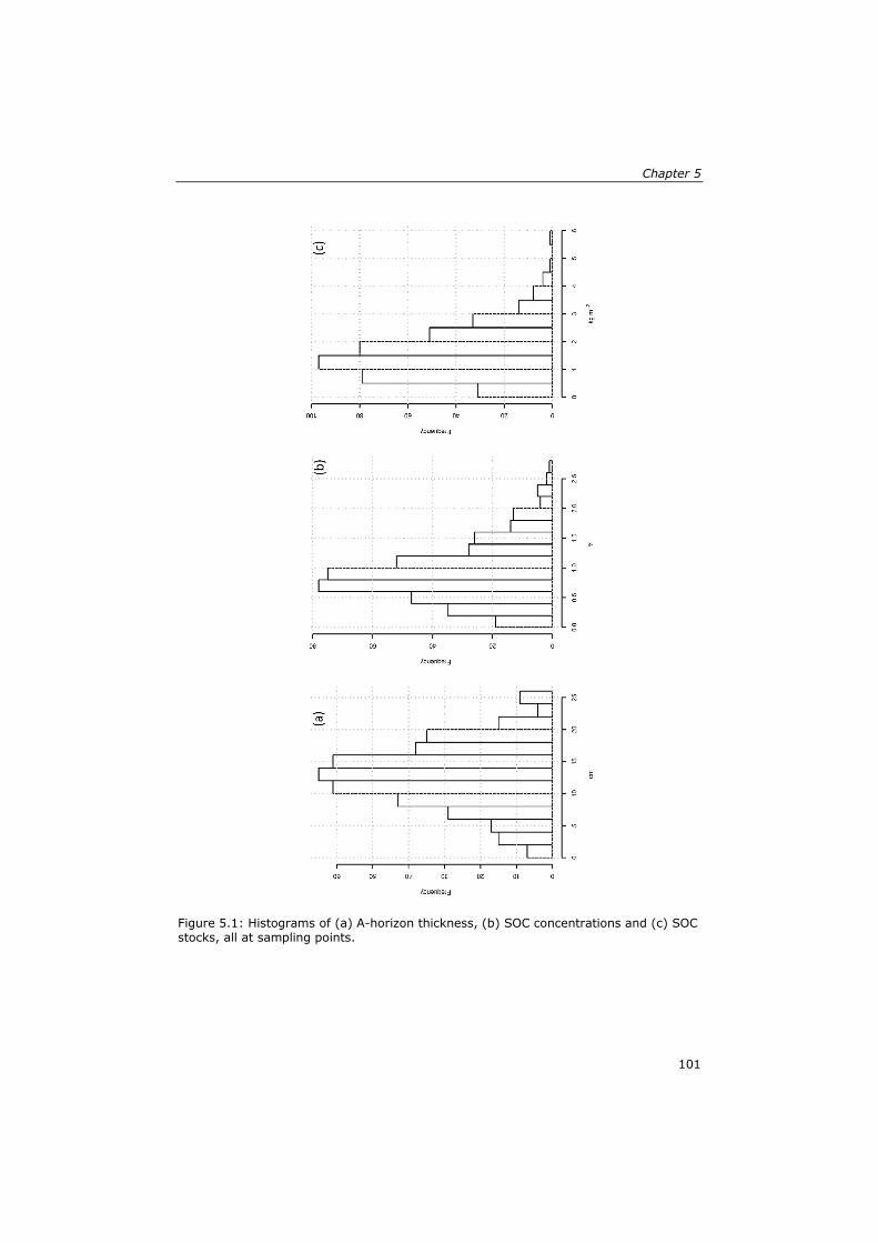
Chapter 5
Figure 5.1: Histograms of (a) A-horizon thickness, (b) SOC concentrations and (c) SOC stocks, all at sampling points.
101

Building a NIR spectral library for the LNP
Figure 5.2: (a) SOC concentration and (b) stocks as a function of A-horizon thickness; (c) relation between SOC stocks and concentration (right). Results for landscape unit NS shown with ‘x’ symbol. The fitted variogram for A-horizon thickness (Table 5.2) shows that its range of spatial dependence almost matches the cluster size. About two-thirds of the variance is spatially-dependent (structural sill vs. total sill). Given this good within-station spatial structure of A-horizon thickness (parameters in
102
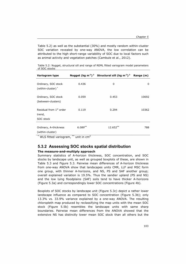
Chapter 5
Table 5.2) as well as the substantial (30%) and mostly random within-cluster SOC variation revealed by one-way ANOVA, the low correlation can be attributed to the high short-range variability of SOC due to local factors such as animal activity and vegetation patches (Cambule et al., 2012). Table 5.2: Nugget, structural sill and range of REML fitted variogram model parameters of SOC stocks
Variogram type Nugget (kg m-2) 2 Structural sill (kg m-2) 2 Range (m)
Ordinary, SOC stock
(within-cluster) *
0.436 0 0
Ordinary, SOC stock
(between-clusters)
0.059 0.453 10692
Residual from 1st order
trend,
SOC stock
0.119 0.294 10362
Ordinary, A-thickness
(within-cluster)
6.089** 12.652** 788
* WLS fitted variogram, ** unit in cm2
5.3.2 Assessing SOC stocks spatial distribution The measure-and-multiply approach Summary statistics of A-horizon thickness, SOC concentration, and SOC stocks by landscape unit, as well as grouped boxplots of these, are shown in Table 5.3 and Figure 5.3. Pairwise mean differences of A-horizon thickness from one-way ANOVA show that landscapes units CMR, LLF and MSC form one group, with thinner A-horizons, and NS, PS and SAF another group; overall explained variation is 19.5%. Thus the sandier upland (PS and NS) and the low lying floodplains (SAF) soils tend to have thicker A-horizons (Figure 5.3a) and correspondingly lower SOC concentrations (Figure 4b). Boxplots of SOC stocks by landscape unit (Figure 5.3c) depict a rather lower landscape influence as compared to SOC concentration (Figure 5.3b); only 13.3% vs. 33.9% variance explained by a one-way ANOVA. The resulting chloropleth map produced by reclassifying the map units with the mean SOC stock (Figure 5.5b) resembles the landscape units with same sharp boundaries. Pairwise mean differences from the ANOVA showed that the extensive NS has distinctly lower mean SOC stock than all others but the
103

Building a NIR spectral library for the LNP
LLF; this latter however is not distinguishable from the others. Thus the fairly homogeneous distribution of stocks across LNP is explained by the negative correlation between SOC concentration and A-horizon thickness. That is, large SOC stocks may have either thick A-horizons or high SOC concentrations (and vice-versa), but rarely both. Within-landscape variation is, however, considerable as shown by the coefficients of variation (Table 5.3); from an overall CV of about 60%, CMR has the lowest and MSC the highest. This heterogeneity may be due to local differences in soil-forming processes that were not recognized or mappable by Stalmans et al. (2004). The differences in sample size per landscape unit also affect the computation: smaller sample sizes give less reliable statistics. Table 5.3: Summary statistics of SOC concentrations, A-horizon thickness and SOC stocks as a function of the landscape unit.
SOC Unit CMR LLF MSC NS PS SAF Number of samples - 14 22 197 98 15 52 SOC concentration* % 1.90 0.91 1.06 0.51 0.92 0.93 SOC concentration SD % 0.36 0.20 0.47 0.26 0.33 0.41 SOC concentration CV % 18.9 22.0 44.3 51.0 35.9 44.1 Area size km2 689 264 4058 4514 253 637 A-horiz. thickness mean cm 9.07 11.11 11.59 15.82 16.53 15.07 A-horiz. thickness SD mean cm 0.86 0.75 0.36 0.41 0.82 0.66 A-horiz. Thickness CV % 35.5 31.5 43.1 25.7 19.1 29.6 SOC stock mean kg m-2 2.46 1.50 1.62 1.13 2.02 2.05 SOC stock SD mean kg m-2 0.25 0.14 0.07 0.06 0.15 0.13 SOC stock CV % 38.6 43.1 57.1 53.5 28.1 46.6 SOC total stocks Gg 1695.9 395.4 6587.7 5081.8 510.3 1307.4
104
Chapter 5
Figure 5.3: Relation of landscape units and (a) A-horizon thickness, (b) SOC stocks and (c) concentration
105

Building a NIR spectral library for the LNP
The soil-landscape approach Explained SOC stocks variation The selected soil-forming explanatory variables are the same as for DSM so their summary statistics were already shown in tab 3.1 (chapter 3). The proportion of SOC stocks variation of all observations explained by the scorpan covariables is about 13.5% (landscape units, i.e., the integrated soil forming factor), 9.5% (coordinates, i.e., geographic trend) and 45% (sampling clusters, i.e., soil factor). Other covariables explained lesser variation, so that a spatial model based on them would not be helpful. When cluster averages were considered, only the coordinates showed increased explanatory power, from 9.5% to about 17%. The obtained amounts of explained variation, from both numerical and categorical explanatory variables, are substantially lower than those obtained for SOC concentration Cambule et al. (2012). That is, the SOC stocks are less variable than SOC concentrations across the study area, which suggests that stocks are mostly in equilibrium with regional climate whereas concentrations vary more with local factors. Spatial structure The result of the within- vs. between-cluster ANOVA shows that the clusters explain about 45% of SOC stocks variation. This is much less between-cluster effect than found for SOC concentration (71.1%) by Cambule et al. (2012). The lower between-cluster stocks variation and its fairly homogeneous spatial distribution (as explained under 4.2.1) may be interpreted as the result of a general equilibrium of SOC stocks with regional climate, i.e., in this environment the net primary production is equal to the litter input to the soil, and the decomposition rate matches these. Visual assessment of the within-cluster variogram (to 720 m) (Figure 5.6a) suggested a very weak spatial dependency to about 300 m with total sill of about 0.44 (kg m-2) 2, quite close to the MSE of the within- vs. between-cluster ANOVA (0.446 kg m-2), which is taken as the residual variance. The total structured variance represents about 0.4% of SOC concentration (Figure 5.2c), about three times the Root Mean Square Error (RMSE) of SOC determination on the base of duplicate samples (0.13%). When the experimental variogram was fitted with a pentaspherical function using WLS fit, an unrealistic zero nugget resulted; this was not improved by the REML. The apparent visible spatial dependence could not be modelled; therefore a pure nugget (0.436 kg m-2) variogram was fitted by WLS (Table 5.2). Consequently the within-cluster SOC stocks variation (about 55%) can be considered as spatially random, i.e., caused by local unmapable factors with high very short-range spatial variability (Janzen and Ellert, 2002; Mapa and Kumaragamage, 1996). Thus the nugget found in the long-range variogram
106

Chapter 5
represents a support of at least a cluster. Therefore the remainder of the analysis is based on the cluster averages.
Figure 5.4: Empirical and fitted variogam models (a) within-cluster, based on all sampling points, (b) between-cluster, based on cluster averages; (c) residuals from first-order trend surface, based on cluster averages.
107

Building a NIR spectral library for the LNP
The long-range (beyond cluster) ordinary experimental variogram showed local spatial dependence to a range of about 20 km (Figure 5.4b). The WLS and REML fitted spherical variograms (separations < 20 km) both showed reasonable structures, with spatial autocorrelation to about 11 km separation (Table 3). This range is about a quarter of the east-west dimension of the LNP, so from the present sample distribution predictions for most of the unsampled areas can only be made by the (spatial) mean, thus giving little insight into spatial variability of SOC stocks. The spherical model was selected based on the patchy structure of spatial variability exhibited by most soil properties. The nugget effect is about 12% of total sill, indicating a high proportion of autocorrelation (Mapa and Kumaragamage, 1996). This low nugget is explained by the averaging effect of clusters, since when the variogram is based on all observations rather than cluster averages, the nugget effect raises to about 43% of the total variance. This is interpreted as the effect of uneven spatial distribution of the “organisms” soil-forming factor (e.g., woody- and non-woody vegetation, termites) as plant production in semi-arid regions depend on small differences on water availability, runoff, infiltration and storage, whose combination results in a very large variation in vegetation and soil properties over small areas (Janzen and Ellert, 2002; Martius et al., 2001; Tiessen and Santos, 1989; Wang et al., 2009); however when this is averaged over a cluster, this variation largely is averaged out. The REML-fitted residual variogram (Table 5.2, Figure 5.4c) for the residuals from a first-order polynomial (the best explanatory variable, representing “spatial position” or local trend) had a range of about 10 km and a nugget effect of 29% of the total sill. Higher-order trend surfaces resulted in lower adjusted goodness-of-fit, and had no obvious interpretation so were not considered. Despite the weak spatial model, a large proportion of spatial dependence spans across a substantial range (> 10 times the cluster length; 720 m), although this range is short relative to the LNP dimensions; thus similarly to the ordinary variogram model, most of unsampled area is predicted by the trend surface, a marginal improvement over the spatial mean. None of beyond-cluster variogram maps showed anisotropy. Selection of spatial prediction model Based on the above result there were the following options for the spatial model: ordinary kriging (OK) considering only the SOC stocks from sampling clusters (“soil”), and universal kriging (UK) with the soil-forming explanatory variable “spatial position” (the coordinates) determining the clear but weak trend. UK is a combination of the standard model of multiple linear regression and the geostatistical methods of ordinary kriging the (trend) residuals (McBratney et al., 2000). The fitted first-order polynomial (plane) represents the trend, whose coefficients (slope in each direction) indicated decrease
108

Chapter 5
towards the NNW. This is interpreted as the effect of decreased annual precipitation and longer dry season in this direction, moving away from the Indian Ocean. SOC stocks distribution in LNP Following the demonstration that within-cluster stocks variation has no spatial structure, cluster averages were used as “points” and therefore the block-kriging was implemented as “punctual” kriging over the practical support of 1x1 km grid, a similar size to the 720x720m clusters. The summary statistics of the SOC stocks across the park by the soil-landscape modelling approach is shown in Table 5.4. Table 5.4: Summary statistics of kriging predictions, kriging prediction standard deviation (SD) and validation results of SOC stocks (kg m-2)
Model Prediction Cross-Validation Validation
Min Median Mean Max SD RMSEP Bias RMSEP Bias
OK 0.71 1.63 1.62 3.53 0.68 0.72 0.01 0.51 -0.35
UK 0.81 1.59 1.59 3.29 0.64 0.69 0.01 0.49 -0.26
The two spatial models predicted similarly as the means differ by about 2%. However OK has larger extreme values, by about 14% and 7% in the lower and higher end, respectively. The maps (Figure 5.5a and c) show clear hot and cold spots. These are unlikely to be true hot/cold spots, rather, the result of limited sampling density relative to the variogram range; thus areas between apparent hot/cold spots are predicted by the spatial mean, resulting in the “pock-marked” map. Both kriged maps show a smooth surface, by contrast to the chloropleth map from the measure-and-multiply approach (Figure 5.5b). The UK map (Figure 5.5c) shows a clear but weak NNW-SSE trend (especially in the higher predictions in the SE corner) and fits well the moderate drop-off in rainfall (Figure 1.2), although adjusted best-fit of linear model of stocks on annual precipitation were not as good as the trend surface. The precipitation surface also takes into account the modest elevation differences (approx. 150 m), which apparently do not improve the relation with SOC.
109

Building a NIR spectral library for the LNP
Figure 5.5: SOC stocks spatial distribution as predicted by (a) ordinary kriging, (b) landscape unit mean and by (c) Universal kriging. Similarly the uncertainty in the estimates (Figure 5.6) is high (CV about 40%) and as is usual for kriging, is much lower near observation points; this effect is more pronounced in OK than UK. In the former, SD is as low as 20% of the mean prediction closer to sampling clusters, rapidly increasing to the maximum SD over most of the study area. The uncertainty of the UK estimates follows a similar pattern, however, with more gradual changes due to the trend surface. The high uncertainty is mainly due to the low sampling density relative to the short-range spatial variation.
Figure 5.6: kriging prediction standard deviation by Universal kriging. Model validation Validation statistics are presented in Table 5. The RMSEP determined by LOOCV is about 44 and 43% of the median of predicted SOC stocks by OK and UK, respectively and therefore poor. OK and UK RMSEP are respectively
110

Chapter 5
about 6 and 8% higher than their mean kriging SD, which is therefore a slightly over-optimistic estimation of the actual error. Refitted spatial models for independent validation were constrained by the reduced number of point-pair within the effective range and the corresponding necessity to make wide bins for the experimental variograms. However, the resulting variograms showed a reasonable structure, with ranges similar to the all-cluster averages variograms. Nugget was however set to 0.0 as REML fit resulted in an unrealistic negative value (Table 5.2). The zero nugget corresponds to the averaging effect of clustered samples. The RMSEP of the independent validation of both spatial models are about 30% of the median predicted SOC stock. When comparing with mean kriging SD, RMSEP is, in both cases, about 35% lower, so kriging SD is a pessimistic measure of the actual prediction error. The models are also biased towards over-prediction, though UK is slightly less so. There are many published studies which estimate SOC stocks; however, in most of these the proportion of the error relative to the range of the predictions is not discussed. Of those that do, the results obtained in this study appear to be slightly better than those obtained in large areas, and as good as those obtained from models applied to smaller areas. In large areas, Mendonça-Santos et al. (2010) estimated the SOC of Rio de Janeiro state (Brazil) in an area of about 44 000 km-2, also following the scorpan-SSPFe framework. Their results show SOC stocks strongly correlated with landscape units and their final map is dominated by SOC stocks < 2.5 kg m-2 and a RMSEP of about 1.2-1.4 kg m-2, i.e., a CV of 50%. Similarly, Mishra et al. (2010) predicted SOC stocks for an area of about 650 00 km-2 in seven midwestern states of the USA, following three methods: multiple linear regression, regression kriging and geographically-weighted regression, obtaining a proportion of RMSE to mean prediction of 103%, 69% and 68%, respectively. Scott et al. (2002) estimated SOC stocks for all of New Zealand based on soil moisture and temperature regimes and landuse. Their findings also show a RMSE proportion of about 44% relative to the mean predictions in sandy soils, but much better (7%) for soils with low-activity clays. In small areas the precision of estimates is somewhat better. For example, Misnasny et al. (2006) estimated SOC stocks in the lower Namoi valley (1 500 km-2) in Australia following the scorpan-SSPFe framework. Their estimates were mostly in the range 2-9 kg m-2 (to 1 m depth) with CV of 30 – 140%. Simbahan et al. (2006) estimated SOC stocks in Nebraska for fields of about 50 – 65 ha using OK, Kriging with external drift, Regression Kriging, and co-kriging, and estimated SOC stocks from 4 to 7 kg m-2 with RMSE from
111
Building a NIR spectral library for the LNP
1.1 and 1.3 kg m-2; for a CV from 17 to 30%. The estimates from present study over a much larger (10 415 km2) area are similar to these. However, the followed soil-landscape modelling approach was not very precise: a RMSEP about 30% the prediction median for both OK and UK. This may be due to the more complex soil-landscape relations at larger areas of the already highly (spatially) variable soil carbon in the landscape (Janzen and Ellert, 2002), justifying the general less precise estimates also found in the literature. It may also be a result of the low sampling density. Nevertheless, in data-poor and poorly accessible areas like LNP study area, achieving comparable results to those from smaller areas shows that the approach is as promising as those based on more comprehensive sampling.
5.3.3 Total SOC stocks estimates and their uncertainty The estimates of total SOC total stocks in LNP are presented in Table 5.5. The results reveal a difference of about 15% between applied methods, being that obtained by summing the landscape totals higher than that from the spatial mean. However, all estimates of the area-normalized mean stock are in a narrow range, 1.59 – 1.62 kg m-2, which is comparable to those reported in the literature for southern Africa. A review by Vagen et al. (2005) reports values for southern Africa savanna soils (to 30 cm depth) between 1 and 1.3 kg m-2 (sandy) and 1.44 to 2 kg m-2 (clay). Williams et al. (2008) studied the SOC stocks of the eastern miombo woodlands soils in Mozambique (to 30 cm depth) and found stocks of about 1.8 to 14 kg m-2. The values are relatively high and may be explained by high leaf litter from leguminous trees (Brachystegia spiciformis), typical of rich miombo vegetation. Ryan et al. (2011b) estimated SOC stocks (to 50 cm depth) in the same vegetation type in Gorongoza District (central Mozambique) at 13.3 kg m-2. The LNP study area is in a much drier environment with less dense vegetation and that of leguminous trees so our figures are much lower.
112

Chapter 5
Table 5.5: Mean SOC stocks, their uncertainty and total stocks, following different approaches
Approach Method Mean
(kg m-2)
SD
(kg m-2)
TOC stock
(Gg)
90% conf.
limit (Gg)
Measure and
multiply
Landscape 1.59 0.45 15 579 ±1 433
naive mean 1.59 0.05 17 828 ±831
Spatial mean 1.60 0.14 17 908 ±2 669
Soil-landscape
modelling
OK 1.62 0.68 16 858 ±11 663
UK 1.59 0.64 16 545 ±10 892
The obtained estimates of SOC stocks by the different methods differ by about 15%, while estimates of the mean SOC stocks only differ by about 2%. This is because of the relative area covered by the different landscape units, each with a different mean stock. This is also corroborated by the wide range between the extreme values of SD (93%), the naive mean having the least dispersion, in contrast to uncertainty estimates from prediction by the spatial models, of which OK is the worse. The naive mean does not account for spatial correlation of the clusters, and thus underestimates the variance, which is thus more realistic when estimated by the spatial mean. The different approaches result in different confidence intervals. The spatially-explicit kriging-based methods of the soil-landscape approach have very wide intervals, 69% (OK) and 65% (UK) of the mean prediction. This is because each grid cell has an uncertainty, and these are not pooled, as in the measure-and-multiply or means approaches. The narrow interval for the naive mean is probably too optimistic, because it does not consider the spatial correlation between observations. Thus the confidence interval based on the spatial mean (15% of the mean prediction) is preferred if only the total stock, not accounting for spatial distribution either over a grid or by landscape unit, is wanted. Despite the differences in confidence intervals and totals, when one is interested in total stocks the measure-and-multiply approach is sufficient given the similarity in the estimates of total stocks. It has also the advantage of not requiring a variogram, which may be difficult to model from a small sample. On the contrary, when interested on the spatial patterns of stocks, then the soil-landscape models are required.
5.3.4 Reliability of SOC stocks estimates and potential improvements
This section discusses the effect of each input on estimates of total stocks, and how each could be improved.
113

Building a NIR spectral library for the LNP
The measurements of A-horizon thickness showed a normal distribution, with a precise estimation of the mean (SD-mean about 2% of the mean), narrow 95% confidence limits (4% of the mean) and few extreme values (5% trimmed mean within 95% confidence limits). The field method is simple and reproducible with an estimated precision of < 0.5 cm in this landscape. There seems to be little room for further improvement, thus its impact on the reliability of estimates is minimal. Laboratory results reported by Cambule et al. (2012), show that SOC concentration measured on 129 samples has an SD of the mean just 6% of the mean, a 95% confidence interval of 12% of the mean, and 5% trimmed mean within 95% confidence limits. Further, RMSE on twenty duplicate samples for quality control was 0.13% SOC, about 15% of the mean and similar to the expected precision for the Walkley-Black method. Again the room for improvement is small. Note however that this results do indirectly influence the PLSR predicted SOC concentration (see further on). The spectrometer used to scan the soil samples has an internal validation test and its spectrum is calibrated before each scan to an internal gold reference. Spectra were only read when internal test was positive. Soil samples were uniformly prepared, and duplicates showed almost no difference in spectra. So it is expected that uncertainty derived from spectroscopy are minimal. Laboratory-measured SOC concentrations were used to build a PLSR calibration model with which estimates were made for the remaining 283 samples. The summary statistics for the entire sample set showed that the SD of the mean was only 3% of the mean (down from the 6% for the laboratory sub-set), the 95% confidence limits were about 5% of the mean and that the 5% trimmed mean fell within the 95% confidence limits of original data. The calibration model had a RMSEP of 0.32% SOC, corresponding to 15% the mean. This uncertainty includes that from the lab analysis of the 129 samples. If the mean stocks would change by 3%, it would still be within the SD-error so it is not expected to affect the 90% confidence intervals. Therefore the estimates made based on spectroscopy can be considered reliable. Bulk density was used to convert SOC from volume concentration to weight and therefore both uncertainty as well as reliability of SOC stock estimates is affected by the BD. In present study the spatial distribution of BD is not known, nor is there a known relation with landscape unit. Only a single value of soil bulk density (1.44 ± 0.02 g.cm-3), derived from nearby measurements and checked against literature, was used. However, given the limited range of SOC concentration (0 – 2.68%, Table 2) and that of the textural classes
114

Chapter 5
(sandy loam to sandy clay loam) from the study area, it seems unlikely that BD could be outside the range 1.4 – 1.65 g cm-3 (EUROCONSULT, 1989). This would correspond to maximum variation in estimated BD of about 15% which would affect the SOC stocks estimates by the same amount. This is more than the SD for the naive and spatial means (SD < 9%) and therefore one could expect that the 90% confidence intervals of total SOC stocks estimated by these methods would also be exceeded. This is then the most unreliable part of the estimate. However, this is a worst-case situation: from obtained estimate of 1.44 g cm-3 to the upper limit 1.65 g cm-3, which would correspond to sandier soils across the entire LNP. This estimate is based on somewhat heavier soils (sandy clay loams) near the confluence of the Singuedzi and Elefant Rivers, similar to the Salvadora angustifolia Floodplains (SAF) map unit, but also from sandy soils from the NS map unit. Thus it seems unlikely that the true mean BD as high as this upper limit, and so the reliability of obtained estimate may not be as poor as this worst-case. Despite the quality control in measurements, the successful PLSR calibration model and the validation statistics for spatial prediction models, the kriged maps have high uncertainty away from sampling locations, and so the reliability of the kriged maps of SOC stock spatial distribution is questionable. This results from a combination of low sampling density and short spatial autocorrelation range relative to study area dimensions. Bulking within-cluster samples at the target grid resolution of 1x1 km would remove the high within-cluster variability. Thus future sampling can be more efficient: only one-seventh of the observations are needed, although some time must be taken in adequately covering the block with a composite sample. With a known variogram, reducing uncertainty in SOC stocking mapping can be aided by the “optimal sampling scheme for isarithmic mapping” (OSSFIM) approach through which the target kriging prediction standard error can be achieved by either (1) reducing the sampling spacing or (2) making predictions over larger blocks (McBratney and Webster, 1981; McBratney et al., 1981). To lower the uncertainty to, e.g., a coefficient of variation of 30% or less (SD ≤ 0.48 kg m-2 on a mean of 1.59 kg m-2), observations would have to be made at maximum 4 km interval for cover the whole area by block universal kriging on 1 km blocks (total of 700, Table 5.6). Similar SD can be obtained by predicting block averages on 5x5 km blocks based on 138 points spaced 9 km apart, i.e., spatial resolution is traded for efficiency. A blocks size smaller than 1x1 km has too much short-range variability to map without very intensive sampling; whether a 1x1 km, 5x5 km or larger block is needed depends on the minimum decision area for management. There is a limit to the efficiency gain, since ground must in any case be traversed. Saving time by bulking the within-cluster samples would make possible to reach further away sampling points.
115

Building a NIR spectral library for the LNP
Table 5.6: Optimal sample spacing for an uncertainty (CV) target of 30% (mean = 1.59 kg m-2)
Block size
(side, m)
Widest
spacing (m)
Achieved
SD (kg m-2)
Number of
observation
points required
1000 4000 0.4361 700
2000 5000 0.4475 448
4000 7000 0.4565 229
5000 9000 0.473 138
7500 20000 0.4325 28
10000 20000 0.3717 28
The sampling points in the regular grid derived from the OSSFIM approach can further be optimized by the spatial simulated annealing, which also allows the minimization of the kriging variance taking into account existing samples (van Groenigen et al., 1999); this would be a sound strategy for a second phase of sampling, starting from the current phase to achieve a target uncertainty. This would however result in a more spread of sampling points which would cost sampling time in exchange for map quality, though not realistic in poorly-accessible areas.
5.4 Conclusions In the present study the total SOC stocks in the LNP was estimated based on limited data collected from accessible areas and have made use of secondary information covering the entire area. The estimates followed both the “measure-and-multiply” and “soil-landscape modelling” approaches. In the former the per stratum mean, the naive mean and the spatial mean, were used while in the latter the ordinary and universal kriging methods, chosen based on the fact that sampling cluster and regional trend were the soil-forming factors that explained SOC stocks variation the most. The mean SOC stocks obtained in all methods are very close however, the SD were distinct, with the soil-landscape modelling methods having at least four times as high SD as the maximum SD for the measure-and-multiply ones. The high uncertainty is mainly due to the short-range spatial variation, by the
116

Chapter 5
sparse sample, the weak trend, and poor correlation with covariables. It would be difficult to improve on this estimate without intensive sampling. The total stocks, obtained by summing (1) the landscape averages and (2) the block-universal-kriged estimates of 1x1 km averages across the whole study area are similar, and also similar to average estimates in soils of similar texture from southern Africa. The high uncertainty of these estimates limit its use as a baseline, however they may be useful for many agricultural studies.
117

Building a NIR spectral library for the LNP
118

Chapter 6 Synthesis and Conclusions
119

Synthesis and Conclusions
6.1 Synthesis and discussion
6.1.1 Renewing legacy soil data for SOC stocks estimation: is it worth the trouble?
Legacy soil data can be a source of data for SOC stocks estimation provided it meets today’s demands in terms of quality. With thorough data archeology many legacy data were uncovered and this can also be the situation in many developing countries. It was based on these data that the recuing, renewal and the testing of its quality following the Cornell adequacy criteria were performed. Chapter 2 established that legacy data can be renewed to some extent and as such the Cornell adequacy criteria proved to be a useful framework for the evaluation of map scale/texture, map legend and positional accuracy of terrain related soil borders. The renewed maps also enabled semi-quantitatively estimation of SOC stocks. However, the poor geodetic control of legacy maps is a main constraint affecting the subsequent renewal steps and quality. Geodetic control of legacy maps with no reference to base map source were made more efficient thanks to the advances of information technology (GIS, computer speed) in combination with thorough data archeology and detective work. The use of GIS made it much efficient to determine the ASD rather than the point count used earlier on. The balance between the gains and pitfalls in legacy data rescue and renewal from present study points to a worthwhile exercise with potential application in developing countries.
6.1.2 Mapping SOC in poorly-accessible areas Effective soil management requires knowledge of the spatial patterns of soil variation within the landscape to enable wise land use decisions. Following Chapter 2 which established that legacy soil data quality could only be improved to some extent through renewal process, the spatial variation of SOC would have to be typically obtained through time-consuming and costly surveys. However, these traditional survey methods are very difficult to implement in poorly-accessible areas. Therefore, chapter 3 developed a cost-efficient methodology for digital soil mapping in such conditions. The methodology is illustrated in an exercise to predict soil organic carbon (SOC) concentration in the Limpopo National Park, Mozambique. The methodology uses a spatial model calibrated on the basis of limited soil sampling and explanatory covariables related to soil-forming factors, developed from readily available secondary information from accessible areas. The model is subsequently applied in the poorly-accessible areas. The methodology is based on three key aspects, namely (i) the similarity of environmental conditions between accessible and poorly accessible areas and
120

Chapter 6
the (ii) sufficiently robust calibration model in accessible areas and, (iii) relative performance of spatial model in poorly-accessible areas. Assessing similarity of environmental conditions between accessible and poorly-accessible areas This first critical stage was here assessed by comparing the mean and the inter quartile range (IQR) for the quantitative covariables and the proportion in which each mapping unit occur in ACC and PACC areas for the categorical covariables. This was a simpler way to compare the two strata. However, more refined and sophisticated methods can be used, depending on availability of the data demanded by the method (Chen et al., 2006; Chen et al., 2008). Chapter 3 established that conditions in the accessible and poorly-accessible areas corresponded sufficiently to allow the extrapolation of the spatial model into the latter. The analysis of similarity in environmental conditions can help target sampling points in accessible areas where samples have higher degree of representativeness of same conditions (and same stratum) in poorly-accessible areas. It is also worth mentioning that this step ensures that the model does not perform satisfactory by chance. Model calibration in accessible areas The predictive model uses the conceptual model scorpan-SSPFe proposed by McBratney et al. (2003) and widely-applied as a generic method for DSM. Scorpan represents the list of soil-forming factors that has been expanded from the original definition by Jenny (1980) representing the initial soil conditions (s), climatic conditions (c), organisms (o) including animals, land cover and human occupation; relief (r), parent material (p), age (a), and the neighbourhood (n). The conceptual model uses a soil spatial prediction function with spatially-autocorrelated errors (SSPFe) that uses (1) a prediction based on environmental covariables and (2) a prediction based on soil properties measured at a limited set of observation points. Readily-available secondary data was used as explanatory variables representing the soil-forming factors. Chapter 3 established that the spatial variation of SOC in the accessible area was mostly described by the sampling cluster (71.5%) and the landscape unit (46.3%). Therefore ordinary (punctual) kriging (OK) and kriging with external drift (KED) based on the landscape unit were used to predict SOC. A linear regression (LM) model using only landscape stratification was used as control. All models were independently validated with test sets collected in accessible areas for which the RMSEP was 0.42-0.50% SOC. Despite the limited utility of the model, given the fact that RMSEP was a substantial proportion predictions median, the subsequent steps were performed to demonstrate the methodology.
121

Synthesis and Conclusions
Relative performance of spatial model in poorly-accessible areas Only sufficiently robust spatial models build based on data from accessible areas should be used to make prediction through into poorly-accessible areas. An independent sample set from poorly-accessible areas was used for validation of all models built in accessible areas. RMSEP was about 0.31-0.36% SOC (Chapter 3). The relative performance as measured by the ratio between the RMSEP in the poorly-accessible and accessible areas was 0.67-0.72, showing that the methodology is predicting SOC in poorly-accessible areas as successful as in accessible areas. Areas with similar problems can thus test the methodology and make predictions if sufficient performance is achieved. This methodology may be also used in baseline studies and for sample design in two-stage surveys. Despite the relatively better model performance in poorly-accessible areas, independent validation from both accessible and poorly-accessible areas were poor, given the fact that independent validation RMSE was a substantial proportion (about half) of the median from models predictions. One way to improve this mapping approach could be, perhaps to calibrate a spatial model per stratum to minimize uncertainty, given the heterogeneity mentioned earlier on. It should be noted that the total number of samples to cover all strata would increase, which could limit validation possibilities in poorly-accessible areas, given the limited number of samples that can be collected. The soil forming factors’ explanatory variables, especially the landscape, were critical for extrapolation into poorly-accessible areas. Without them it would have been much more difficult to make prediction, given the limited number of samples that can be collected there. Therefore, robust soil-forming explanatory variables are helpful and should be explored for DSM mapping of poorly-accessible environments.
6.1.3 Near-infrared spectroscopy: a rapid, non-destructive and environmentally friendly lab method
Soil organic carbon (SOC) is a key soil property and particularly important for ecosystem functioning and the sustainable management of agricultural systems. Soil surveys rely on large number of soil samples to reveal the spatial patterns of soil properties. Traditional laboratory methods to analyse these samples are time-consuming and costly. Many authors claim that laboratory spectroscopy in combination with chemometrics to be a rapid, non-
122

Chapter 6
destructive, environmentally friendly and inexpensive soil analysis for SOC determination. However, they require calibration of robust models which also require a large number of samples. Unfortunately in poorly-accessible areas only a limited number of soil samples can be collected, which constitutes a challenge for calibrating of a robust model. Chapter 3 calibrated a PLSR-NIR model later used for DSM mapping. Calibration of PLSR-NIR model One third (129) of soil samples collected for DSM in the LNP (chapter 3) were selected for reference analysis, lab-NIR spectral signature acquisition and subsequent building of PLSR-NIR calibration model. Selection was made on the base of their spectral diversity using a combination of PCA and K-means clustering techniques. Model calibration accuracy was evaluated by RMSE of calibration of the cross-validation predictions, and R2 of the SOC vector. Prediction accuracy was assessed by the RPD of cross-validation and by the multiple R2 (Chang et al., 2001; Waiser et al., 2007). Partial least square regression (PLSR) was used on 1037 bands in the wavelength range 1.25 – 2.5 µm to relate the spectra and SOC concentration. Several models were built and compared by cross-validation. The best model was on a filtered first derivative of the multiplicative scatter corrected (MSC) spectra. It explained 83% of SOC variation and had a root mean square error of prediction (RMSEP) of 0.32% SOC, about 2.5 times the laboratory RMSE from duplicate samples (0.13% SOC). This uncertainty is a substantial proportion of the typical SOC concentrations in LNP landscapes (0.45 – 2.00%). The model was slightly improved (RMSEP 0.28% SOC) by adding clay percentage as a co-variable. All models had poorer performance (under-prediction) at SOC concentrations above 2.0%, indicating a saturation effect. Chapter 3 established then that despite the limitations of sample size and no pre-existing library, a locally-useful, although somewhat imprecise, calibration model could be built. This model is suitable for estimating SOC in further mapping exercises in the LNP. This comes in hand to support soil survey in poorly-accessible areas. Prediction of SOC using PLSR-NIR calibrated model The 412 soil samples for DSM were scanned for NIR spectral signature acquisition and the calibration model just obtained was used to predict SOC concentration. Chapter 3 reports prediction of SOC for the entire sample set, using PLSR-NIR calibrated model (chapter 4). Here the model also tended to under-estimate at the higher end (1.5-1.8%) however, the proportion of under-estimated samples was slightly smaller (6%) compared to observed under-prediction on reference wet laboratory sample sets (7%). The
123

Synthesis and Conclusions
predicted SOC at sampling points was further used to build the spatial model with which was predicted the LNP SOC spatial distribution.
6.1.4 SOC stocks in LNP; amount, spatial distribution and uncertainty
Many areas in sub-Saharan African are data-poor and poorly accessible so mapping Soil Organic Carbon (SOC) stocks in these areas will have to rely on the limited available secondary data coupled with restricted field sampling. SOC spatial distribution is a function of the interaction of the soil-forming factors as described by Jenny (1980). It was here modelled based on limited available secondary data coupled with restricted field sampling and following two approaches: the i) measure-and-multiply by landscape unit and ii) soil-landscape model following the predictive conceptual model scorpan-SSPFe McBratney et al. (2003) which uses a soil spatial prediction function with spatially-autocorrelated errors (SSPFe) that uses (1) a prediction based on environmental covariables and (2) a prediction based on soil properties measured at a limited set of observation points. It is widely-applied as a generic method for DSM. During field survey A-horizon thickness measurements were made and soil samples taken for the determination of SOC concentrations. SOC concentrations were multiplied by soil bulk density and A-horizon thickness to estimate SOC stocks. An average BD was used and it was based on earlier measurements in part of the study area (the extensive NS landscape), reported by COBA Consultores (1982) and was crosschecked in the literature (EUROCONSULT, 1989) for similar soils, resulting in expected maximum BD variation of about 15% and equal impact on SOC stocks estimates in a worse-case situation. Chapter 5 established that spatial distribution of SOC stock in the LNP was rather homogeneous (suggesting levels are mainly determined by regional climate); mean SOC stock from all sample points is 1.59 kg m-2; landscape unit averages are 1.13 - 2.46 kg m-2. Covariables explained 45% (“soil”) and 17% (coordinates) of SOC stock variation. Predictions from spatial models averaged 1.65 kg m-2 and are smoother, though with clear hot/cold spots due to limited sampling density across LNP. These results are within the ranges reported for similar soils in southern Africa (Ryan et al., 2011; Vågen et al., 2005; Williams et al., 2008). The RMSEP was about 30% of the mean predictions for both OK and UK. Uncertainty is high (CV of about 40%) due to short-range spatial structure combined with sparse sampling. The range of total SOC stock of the 10 410 km-2 study area was estimated at 15 579 - 17 908 Gg. However, 90% confidence limits of the total stocks estimated are narrower (5 – 15%) for the measure-and-multiply and wider (66 - 70%) for
124

Chapter 6
the soil-landscape model due to the short-range spatial variation, the sparse sample, the weak trend, and poor correlation with covariables. The expected impact of BD uncertainty on SOC stocks also contributed to these wider 90% confidence limits and thus affecting the reliability of the estimates. The chapter also established that improving these estimates would be difficult without intensive sampling. However, bulking within-cluster samples at the target grid resolution of 1x1 km would remove the high within-cluster variability and thus future sampling can be more efficient. Now that the variogram is known, reducing uncertainty in SOC stocks mapping to a desired level can be achieved by either (1) reducing the sampling spacing or (2) making predictions over larger blocks. This can be aided by the “optimal sampling scheme for isarithmic mapping” (OSSFIM) (McBratney and Webster, 1981; McBratney et al., 1981). Nevertheless, the results from this study are below the typical levels of SOC stocks (30 cm depth) typically found in arid environments or on arenosols, namely about 2.0 – 2.2 kgm-2 (FAO, 2001) by, about 20-25%. This may be due to the effect of nutrient-poor sands and also poor land use management, leading to lower levels.
6.2 Concluding remarks The Cornell adequacy criteria here tested to assess legacy survey renewal quality proved to be a guiding framework to consider in legacy survey data renewal. As such it has a potential to screen shelved and almost forgotten wealth of legacy surveys to bring back quality data into use. The proposed DSM methodology for mapping poorly-accessible areas is promising because it did work as planned in the sense that the models did as well in poorly-accessible as in accessible areas. One of the strong points of the obtained results lies on the long spatial models’ range, which allows interpolation into PACC. This is despite the poor model predictions result, which were due to cumulative error effects brought about along the different steps, namely laboratory analysis, PLSR calibration, model building. The use of a previous integrative survey by Stalmans et al. (2004) was quite helpful in this case and was able to substitute for multiple factors (soil-forming explanatory variables) in the scorpan-SPPfe framework. This implies that a previous study, stratifying an area to be surveyed by major soil-forming factors, can be a valuable first step before any geostatistical sampling. SOC concentration in the study area varies mostly by local factors, probably current and past vegetation and animal activity (including termites), not
125

Synthesis and Conclusions
captured by any covariable. The range of SOC concentrations was narrow, weakly-dependent on covariables, and exhibited most of its spatial structure within the support of a cluster. A locally-useful PLSR-NIR calibration model based on limited sample size and no pre-existing library could be built and is suitable for estimating SOC in further mapping and monitoring exercises in the LNP. The model is somewhat imprecise for monitoring, but still cost-effective. The inclusion of clay percentage (a moderately-correlated covariable) in the set of predictors slightly improved the precision. The two approaches followed to assess the spatial distribution of SOC stocks resulted in closer SOC mean values however; they had distinct uncertainty, with soil-landscape modelling methods showing the highest. This is mainly due to the short-range spatial variation, by the sparse sample, the weak trend, and poor correlation with covariables. In this situation, improving the estimates require intensive sampling. The high uncertainty of these estimates limits its use as a baseline; however they may be useful for many agricultural studies. The estimated total stocks, obtained following both approaches for the whole study area are similar, and also similar to average estimates in soils of similar texture from southern Africa. However and similar to SOC concentrations they show high uncertainty which limit its use as a baseline, however they may be useful for many agricultural studies.
6.3 Recommendations
6.3.1 Application of the results of this study The renewal of legacy soil maps following the stepwise DSM approach by Rossiter (2008) made it easier to test the Cornell adequacy criteria as data renewal evaluation criteria. Therefore its implementation can be recommended either to bring most out of legacy data in data-poor or to support new (re)surveys. The criteria have a potential for a wider use as a result of recent advances in information technology and computer speed, which make their applicability more efficient. The stepwise methodology for digital soil mapping in poorly-accessible areas as proposed in present study can be applied easily elsewhere and as such can aid in mapping soil properties in similar areas, provided soil-forming explanatory variables that explain substantial amount of soil property variation are available. Integrative surveys like the one by Stalmans et.al. (2004) are good examples that can also be used as soil-forming explanatory
126

Chapter 6
variable, especially for poorly-accessible and data-poor environments. However, such surveys require integrative expertise, on landscape processes, which in any case is needed for intelligent management. The use of NIR to largely replace wet laboratory determinations is becoming routine. However, in areas with no previous calibration, such as the LNP, there remains the question as to how easily a calibration can be built. LNP is such a pioneer area with no previous spectral library, yet the present modestly-sized study was able to obtain a reasonable calibration. This is encouraging for similar studies of pioneer areas. From the current study, following the approach brought about by present study can aid in building a wider Mozambican soil spectral library which would enhance the robustness of calibration model. The present study demonstrated that the use correlated covariable (e.g. clay) in the set of predictors can improve the precision of PLSR-NIR calibration models. This approach can be applied with other correlated covariables to improve calibration models in future. This may result in cost-effective, rapid and environmental friendly laboratory analysis of several soil properties. The methodology for total SOC stocks estimation here followed; especially for spatial model building can be easily applied to other areas to estimate total SOC stocks. This is important in the context of climate change mitigation, e.g.: for the estimation of the carbon sink capacity and SOC sequestration. The importance of bulk density measurement is clear here; any method to make this more efficient would greatly enhance TOC studies.
6.3.2 Recommendations for further research Semi-detailed legacy soil surveys were carried out following free survey methods and physiographic approach for map unit definition. Available algorithms for the extraction of physiographic units are limited to at lower scale maps and therefore poorly perform in floodplains type of landscapes where many legacy soil surveys were carried out to support land development (irrigation schemes). Therefore research should be also targeted the refinement of such algorithms to support legacy data renewal in these environments. Given the poor DSM prediction results (SOC concentration), it would be worth to investigate the sampling plan that would improve the estimates. This could be achieved by e.g. optimizing the KED variance to a realistic target (e.g. the one set by PLSR precision) as suggested by Brus and Heuvelink (2007). This would be supported by now known spatial structure and relation of target variable with covariables, and there is evidence that the model structure in poorly-accessible areas is likely to be similar to that in accessible areas. It
127

Synthesis and Conclusions
was also demonstrated that it is not work mapping smaller areas, instead is better to sample on a 1 km support given the fact that below that variation is high and unstructured. However that would imply that management decisions would be on a 1 km block size. This would be adequate for general land-use planning, e.g., siting of settlements; within identified areas detailed surveys could be carried out. The precision level of NIR calibration models obtained here have potential for SOC prediction in regional and baseline studies, however they cannot be used for detailed ecological and farm-level studies within the LNP or in similar nearby soil landscapes. Therefore it would be worth testing as whether spiking the models (recalibration after adding a few “local” samples) would improve precision as demonstrated elsewhere (Guerrero et al., 2010). It was observed from the results that both NIR-PLSR calibration models (normal and inclusion of clay) under-predicted at the extreme values with emphasis to the higher extreme values due to a “banana-like” model trend. Therefore it would worth to investigate as whether non-linear PLS could remove the observed non-linear trend, to improved predictions. The chosen sampling plan for soil collection was designed for soil mapping. It was designed following random cluster to capture more efficiently the local and regional spatial variation. However, the same samples were also used to build the PLSR-NIR calibration model by selecting samples based on PCA score grouping for reference analysis. Whereas PCA score grouping enhances spectral diversity, it may also enhance the spatial autocorrelation between the selected samples due to possible coincidence of PCA score groups with the field sample clusters. This raises the possibility of false precision as noted by Brown et al. (2005). In situations where few samples can be collected “false precision” imposes limitation for this combination analysis. Therefore alternative approaches are needed. The BD was the main source of uncertainty in the SOC stocks estimates. It is therefore recommended to investigate as to what extent BD is causing the high uncertainty, perhaps by taking measurements of BD to represent its real spatial distribution in the LNP. Further, efficient methods for determining BD in-situ should be investigated. It is also recommended to investigate what could be best soil-forming explanatory variables to be used as predictors in the spatial model as all (except landscape and coordinates, also week) selected here did not explain substantial SOC variation and therefore were not helpful for model calibration.
128

References Ahmed, F.B., Dent, D.L., 1997. Resurrection of soil surveys: a case study of
the acid sulphate soils of The Gambia. II. Added value from spatial statistics. Soil use and management 13, 57-59.
Amichev, B.Y., Galbraith, J.M., 2004. A Revised Methodology for Estimation of Forest Soil Carbon from Spatial Soils and Forest Inventory Data Sets. Environmental Management 33(0), S74-S86.
Antle, J.M., Stoorvogel, J.J., Valdivia, R.O., 2007. Assessing the economic impacts of agricultural carbon sequestration: Terraces and agroforestry in the Peruvian Andes. Agriculture, Ecosystems & Environment 122(4), 435-445.
Arshad, M.A., Martin, S., 2002. Identifying critical limits for soil quality indicators in agro-ecosystems. Agriculture, Ecosystems & Environment 88(2), 153-160.
Aubry, P., Debouzie, D., 2000. Geostatistical Estimation Variance for the Spatial Mean in Two-Dimensional Systematic Sampling. Ecology 81(2), 543-553.
Batjes, N.H., 2008. Mapping soil carbon stocks of Central Africa using SOTER. Geoderma 146(1-2), 58-65.
Batjes, N.H., Al-Adamat, R., Bhattacharyya, T., Bernoux, M., Cerri, C.E.P., Gicheru, P., Kamoni, P., Milne, E., Pal, D.K., Rawajfih, Z., 2007. Preparation of consistent soil data sets for modelling purposes: Secondary SOTER data for four case study areas. Agriculture, Ecosystems & Environment 122(1), 26-34.
Batjes, N.H., and E.M. Briges, 1992. A review of soil factors and processes that control fluxes of heat, moisture and greenhouse gases. Tecnical paper. International Soil Reference and Information Centre 23.
Baxter, S.J., Crawford, D.M., 2008. Incorporating legacy soil pH databases into digital soil maps. In: A. Hartemink, A. McBratney, M.L. Mendonça-Santos (Eds.), Digital soil mapping with limited data. Springer, pp. 311-318.
Ben-Dor, E., 2002. Quantitative remote sensing of soil properties, Advances in Agronomy. Academic Press, pp. 173-243.
Ben-Dor, E., Banin, A., 1990. Near-Infrared reflectance analysis of Carbonate concentration in soils. Applied Spectroscopy 44, 1064-1069.
Ben-Dor, E., Banin, A., 1995. Near-Infrared analysis as a rapid method to simultaneously evaluate several soil properties. Soil Science Society of America Journal 59, 364-372.
Ben-Dor, E., Irons, J.R., Epema, G.F., 1999. Soil reflectance. In: A.N. Rencz (Ed.), Remote sensing for earth sciences. Manual of remote sensing. John Wiley & Sons, Inc., Toronto, pp. 111-188.
129
References
Bhatti, A.U., Mulla, D.J., Frazier, B.E., 1991. Estimation of soil properties and wheat yields on complex eroded hills using geostatistics and thematic mapper images. Remote Sensing of Environment 37(3), 181-191.
Bouma, J., 2002. Land quality indicators of sustainable land management across scales. Agriculture, Ecosystems & Environment 88(2), 129-136.
Brown, D.J., 2007. Using a global VNIR soil-spectral library for local soil characterization and landscape modeling in a 2nd-order Uganda watershed. Geoderma 140(4), 444-453.
Brown, D.J., Bricklemyer, R.S., Miller, P.R., 2005. Validation requirements for diffuse reflectance soil characterization models with a case study of VNIR soil C prediction in Montana. Geoderma 129(3-4), 251-267.
Brown, D.J., Shepherd, K.D., Walsh, M.G., Dewayne Mays, M., Reinsch, T.G., 2006. Global soil characterization with VNIR diffuse reflectance spectroscopy. Geoderma 132(3-4), 273-290.
Brus, D.J., Heuvelink, G.B.M., 2007. Optimization of sample patterns for universal kriging of environmental variables. Geoderma 138(1-2), 86-95.
Cambule, A.H., Rossiter, D.G., Stoorvogel, J.J., 2013. A methodology for digital soil mapping in poorly accessible areas. Geoderma 192, 341-351.
Cambule, A.H., Rossiter, D.G., Stoorvogel, J.J., Smaling, E.M.A., 2012. Building a near infrared spectral library for soil organic carbon estimation in the Limpopo National Park, Mozambique. Geoderma 183-184, 41-48.
Cambule, A.H., Rossiter, D.G., Stoorvogel, J.J., Smaling, E.M.A., (under review). Soil Organic Carbon stocks in the Limpopo National Park, Mozambique: amount, spatial distribution and uncertainty. Geoderma.
Casimiro, J.d.F., Veloso, A.P., 1969. Levantamento de solos da margem esquerda do Rio dos Elefantes e sua aptidão para o regadio (Zona a montante da confluência com o Rio Chinguidzi), Grupo de trabalho do Limpopo.
Cécillon, L., Barthès, B.G., Gomez, C., Ertlen, D., Genot, V., Hedde, M., Stevens, A., Brun, J.J., 2009a. Assessment and monitoring of soil quality using near-infrared reflectance spectroscopy (NIRS). European Journal of Soil Science 60(5), 770-784.
Cécillon, L., Cassagne, N., Czarnes, S., Gros, R., Vennetier, M., Brun, J.-J., 2009b. Predicting soil quality indices with near infrared analysis in a wildfire chronosequence. Science of The Total Environment 407(3), 1200-1205.
Chang, C.-W., Laird, D.A., Mausbach, M.J., Hurburgh, C.R., Jr., 2001. Near-Infrared Reflectance Spectroscopy-Principal Components Regression Analyses of Soil Properties. Soil Sci Soc Am J 65(2), 480-490.
130

References
Chatterjee, A., Lal, R., Wielopolski, L., Martin, M.Z., Ebinger, M.H., 2009. Evaluation of Different Soil Carbon Determination Methods. Critical Reviews in Plant Sciences 28(3), 164 - 178.
COBA Consultores, 1981. Aproveitamento hidroagrícola de Massingir-Chinhangane - Carta dos Solos, Carta de Aptidão para Regadio, SERLI, Maputo.
COBA Consultores, 1982. Aproveitamento hidroagrícola de Massingir-Chinhangane, SERLI, Maputo.
COBA Consultores, 1983a. Aproveitamento hidroagrícola de Chibotane-Machaul-Madingane, SERLI, Maputo.
COBA Consultores, 1983b. Desenvolvimento das Aldeias Comunais de Cubo, Paulo Samuel Kankomba, Massingir-velho e Mavodze - Carta dos Solos e do Potencial Agrícola, Carta das Pastagens e do Potencial Florestal, SERLI, Maputo.
De Gruijter, J.J., Brus, D.J., Bierkens, M.F.P., Knotters, M., 2006. Sampling for Natural Resource Monitoring. Springer, Berlin.
Dent, D.L., Ahmed, F.B., 1995. Resurrection of soil surveys: a case study of the acid sulphate soils of The Gambia. I. Data validation, taxonomic and mapping units. Soil use and management 11, 69-76.
Dijkshoorn, J.A., 2003. SOTER database for southern Africa, International Soil Reference and Information Centre.
Esbensen, K., 1994. Multivariate data analysis in practice. CAMO Software AS, Oslo.
EUROCONSULT, 1989. Agricultural compendium for rural development in the tropics and subtropics. Third revised edition ed. Elsevier Scientific, Amsterdam etc.
FAO, 2001. Soil carbon sequestration for improved land management. ISBN 92-5-104690-5, ISSN 0532-0488, FAO, Rome.
FAO, Unesco, ISRIC, 1997. FAO - Unesco Soil map of the world - Revised legend with corrections and updates, International soil reference centre.
Fearn, T., 2010. Combining other predictors with NIR spectra. Chemometric Space 21(2), 13-16.
Fidêncio, P.H., Poppi, R.J., de Andrade, J.C., 2002. Determination of organic matter in soils using radial basis function networks and near infrared spectroscopy. Analytica Chimica Acta 453(1), 125-134.
Florinsky, I.V., Eilers, R.G., Manning, G.R., Fuller, L.G., 2002. Prediction of soil properties by digital terrain modelling. Environmental Modelling & Software 17(3), 295-311.
Forbes, T.R., Rossiter, D.G., Van Wambeke, A., 1982. Guidelines for evaluating the adequacy of soil resource invenctories, Cornell University Department of Agronomy, New York.
Fox, J., 1997. Applied regression, linear models, and related methods. Sage, Newbury Park.
131

References
Franklin, R.B., Mills, A.L., 2003. Multi-scale variation in spatial heterogeneity for microbial community structure in an eastern Virginia agricultural field. FEMS Microbiology Ecology 44, 335-346.
Fystro, G., 2002. The prediction of C and N content and their potential mineralisation in heterogeneous soil samples using Vis–NIR spectroscopy and comparative methods. Plant and Soil 246(2), 139-149.
Gallant, J.C., Wilson, J.P., 1996. TAPES-G: A grid-based terrain analysis program for the environmental sciences. Computers & Geosciences 22(7), 713-722.
Geladi, P., Kowalski, B.R., 1986. Partial least-squares regression: a tutorial. Analytica Chimica Acta 185, 1-17.
Gessler, P.E., Chadwick, O.A., Chamran, F., Althouse, L., Holmes, K., 2000a. Modeling Soil-Landscape and Ecosystem Properties Using Terrain Attributes. Soil Sci Soc Am J 64(6), 2046-2056.
Gessler, P.E., Chadwick, O.A., Chamran, F., Althouse, L., Holmes, K., 2000b. Modeling Soil–Landscape and Ecosystem Properties Using Terrain Attributes. Soil Science Society of America Journal 64, 2046-2056.
Gijsman, A.J., Jagtap, S.S., Jones, J.W., 2002. Wading through a swamp of complete confusion: how to choose a method for estimating soil water retention parameters for crop models. European Journal of Agronomy 18(1-2), 77-106.
Giller, K.E., Leeuwis, C., Andersson, J.A., Andriesse, W., Brouwer, A., Frost, P., Hebinck, P., Heitkonig, I., van Ittersum, M.K., Koning, N., Ruben, R., Slingerland, M., Udo, H., Veldkamp, T., van de Vijver, C., van Wijk, M.T., Windmeijer, P., 2008. Competing Claims on Natural Resources: What Role for Science? Ecol. Soc. 13(2), 18.
Gisladottir, G., Stocking, M., 2005. Land degradation control and its global environmental benefits. Land Degradation & Development 16, 99–112.
Gitelson, A.A., Merzlyak, M.N., 1998. Remote sensing of chlorophyll concentration in higher plant leaves. Advances in Space Research 22(5), 689-692.
Godinho Gouveia, D.H., Azevedo, Á.L., 1954. The Provisional Soil Map of Moçambique, Abstract of the Proceedings of the 2nd Inter-African Soils Conference, Leopoldville pp. 1459 - 1468.
Godinho Gouveia, D.H., Azevedo, Á.L., 1955a. Características e distribuição dos solos de Moçambique: I - Carta provisória dos solos do sul de Save, II - Esboço pedológico da colónia de Moçambique, Centro de investigação científica algodoeira.
Godinho Gouveia, D.H., Azevedo, Á.L., 1955b. Os Solos. In: Junta de Exportaçao do Algodao (Ed.), Esboço de reconhecimento ecológico-agrícola de Moçambique. Memórias e Trabalhos. Centro de Investigação Científica Algodoeira, Lourenço Marques, pp. 3-56.
132

References
Godinho Gouveia, D.H., Marques, A.S.e.M., 1973. Carta de solos de Moçambique (Esc. 1 : 4 000 000). Agronomia Moçambicana 7(1), 1-68.
Goodchild, M.F., Hunter, G.J., 1997. A simple positional accuracy measure for linear features. International Journal of Geographical Information Science 11(3), 299-306.
Goovaerts, P., 1999. Geostatistics in soil science: state-of-the-art and perspectives. Geoderma 89(1-2), 1-45.
Grimm, R., Behrens, T., Märker, M., Elsenbeer, H., 2008. Soil organic carbon concentrations and stocks on Barro Colorado Island -- Digital soil mapping using Random Forests analysis. Geoderma 146(1-2), 102-113.
Grinand, C., Arrouays, D., Laroche, B., Martin, M.P., 2008. Extrapolating regional soil landscapes from an existing soil map: Sampling intensity, validation procedures, and integration of spatial context. Geoderma 143(1-2), 180-190.
Gringarten, E., Deutch, C.V., 2001. Teacher's aid variogram interpretation and modeling. Mathematical Geology 33(4), 507-534.
Grupo de trabalho de Limpopo, Undated. Levantamento de solos da margem direita do Rio ddos Elefantes (Marrenguele-Banga), Gabinete do Limpopo, Lourenço Marques.
Guerrero, C., Zornoza, R., Gómez, I., Mataix-Beneyto, J., 2010. Spiking of NIR regional models using samples from target sites: Effect of model size on prediction accuracy. Geoderma 158(1-2), 66-77.
Guo, Y., Amundson, R., Gong, P., Yu, Q., 2006. Quantity and Spatial Variability of Soil Carbon in the Conterminous United States. Soil Sci. Soc. Am. J. 70(2), 590-600.
Hartemink, A.E., McBratney, A.B., Mendonça-Santos, M.L., 2008. Digital soil mapping with limited data. Springer.
Hendriks, P.H.J., Dessers, E., Hootegem, G.v., 2012. Reconsidering the definition of a spatial data infrastructure. International Journal of Geographical Information Science 26(8), 1479-1494.
Hengl, T., 2006. Finding the right pixel size. Computers & Geosciences 32(9), 1283-1298.
Hengl, T., Heuvelink, G.B.M., Rossiter, D.G., 2007. About regression-kriging: From equations to case studies. Computers & Geosciences 33(10), 1301-1315.
Hengl, T., Rossiter, D.G., 2003. Supervised Landform Classification to Enhance and Replace Photo-Interpretation in Semi-Detailed Soil Survey. Soil Sci Soc Am J 67(6), 1810-1822.
Heuvelink, G.B.M., Webster, R., 2001. Modelling soil variation: past, present, and future. Geoderma 100(3-4), 269-301.
Hijmans, R.J., Cameron, S., Parra, J., 2011. WorldClim - Global Climate Data, Berkley, CA.
133

References
Hughes, M.L., McDowell, P.F., Marcus, W.A., 2006. Accuracy assessment of georectified aerial photographs: Implications for measuring lateral channel movement in a GIS. Geomorphology 74(1–4), 1-16.
Ihaka, R., Gentleman, R., 1996. R: A Language for Data Analysis and Graphics. Journal of Computational and Graphical Statistics 5(3), 299--314.
Iliffe, J., Lott, R., 2008. Datums and map projections for remote sensing, GIS, and surveying. Whittles Pub.; CRC Press, Scotland, UK; Boca Raton, FL.
Janssen, B.H., Guiking, F.C.T., van der Eijk, D., Smaling, E.M.A., Wolf, J., van Reuler, H., 1990. A system for quantitative evaluation of the fertility of tropical soils (QUEFTS). Geoderma 46(4), 299-318.
Janssen, P.H.M., Heuberger, P.S.C., 1995. Calibration of process-oriented models. Ecological Modelling 83(1-2), 55-66.
Janzen, H.H., Ellert, B.H., 2002. Organic matter in the landscape. In: R. Lal. (Ed.), Encyclopedia of soil science M. Dekker inc, New York, pp. 905-909.
Jenny, H., 1980. The soil resource : origin and behavior. Ecological Studies 37. Springer-Verlag, New York.
Kiiveri, H.T., 1997. Assessing, representing and transmitting positional uncertainty in maps. International Journal of Geographical Information Science 11(1), 33-52.
Krol, B.G.C.M., 2008. Towards a data quality management framework for digital soil mapping with limited data. In: A. Hartemink, A. McBratney, M.L. Mendonça-Santos (Eds.), Digital soil mapping with limited data. Springer, pp. 137-149.
Lagacherie, P., McBratney, A.B., Voltz, M., 2007. Digital soil mapping : an introductory perspective. Developments in soil science, 13. Elsevier, Amsterdam etc.
Lark, R.M., 2002. Optimized spatial sampling of soil for estimation of the variogram by maximum likelihood. Geoderma 105(1-2), 49-80.
Leenars, J.G.B., 2012. Africa Soil Profiles Database, Version 1.0. A compilation of geo-referenced and standardized legacy soil profile data for Sub Saharan Africa (with dataset). ISRIC Report No. 2012/03.
Liu, D., Wang, Z., Zhang, B., Song, K., Li, X., Li, J., Li, F., Duan, H., 2006. Spatial distribution of soil organic carbon and analysis of related factors in croplands of the black soil region, Northeast China. Agriculture, Ecosystems & Environment 113(1-4), 73-81.
MacMillan, R.A., Pettapiece, W.W., Nolan, S.C., Goddard, T.W., 2000. A generic procedure for automatically segmenting landforms into landform elements using DEMs, heuristic rules and fuzzy logic. Fuzzy Sets and Systems 113(1), 81-109.
134

References
Manninen, T., Eerola, T., Makitie, H., Vuori, S., Luttinen, A., Senvano, A., Manhica, V., 2008. The Karoo volcanic rocks and related intrusions in southern and central Mozambique. Geological Survey of Finland, Special Paper 48, 211-250.
Mapa, R.B., Kumaragamage, D., 1996. Variability of soil properties in a tropical Alfisol used for shifting cultivation. Soil Technology 9(3), 187-197.
Marchant, B.P., Lark, R.M., 2007. Robust estimation of the variogram by residual maximum likelihood. Geoderma 140(1-2), 62-72.
Martens, H., Naes, T., 1986. Multivariate calibration. John Wiley & Sons, Chichester.
Martius, C., Tiessen, H., Vlek, P.L.G., 2001. The management of organic matter in tropical soils: what are the priorities? Nutrient Cycling in Agroecosystems 61(1), 1-6.
McBratney, A.B., Mendonca Santos, M.L., Minasny, B., 2003. On digital soil mapping. Geoderma 117(1-2), 3-52.
McBratney, A.B., Odeh, I.O.A., Bishop, T.F.A., Dunbar, M.S., Shatar, T.M., 2000. An overview of pedometric techniques for use in soil survey. Geoderma 97(3-4), 293-327.
McBratney, A.B., Webster, R., 1981. The design of optimal sampling schemes for local estimation and mapping of regionalized variables--II: Program and examples. Computers & Geosciences 7(4), 335-365.
McBratney, A.B., Webster, R., Burgess, T.M., 1981. The design of optimal sampling schemes for local estimation and mapping of of regionalized variables--I: Theory and method. Computers & Geosciences 7(4), 331-334.
McGrath, D., Zhang, C., 2003. Spatial distribution of soil organic carbon concentrations in grassland of Ireland. Applied Geochemistry 18(10), 1629-1639.
McKenzie, N.J., Gessler, P.E., Ryan, P.J., O'Connell, D.A., 2000. The role of terrain analysis in soil mapping. In: J.P. Wilson, J. Gallant (Eds.), Terrain analysis : principles and applications. Wiley & Sons, New York, pp. 245-265.
Mevik, B.-H., Wehrens, R., 2007. The pls Package: Principal Component and Partial Least Squares Regression in R. Journal of Statistical Software 18(2), 1-24.
Milne, E., Adamat, R.A., Batjes, N.H., Bernoux, M., Bhattacharyya, T., Cerri, C.C., Cerri, C.E.P., Coleman, K., Easter, M., Falloon, P., Feller, C., Gicheru, P., Kamoni, P., Killian, K., Pal, D.K., Paustian, K., Powlson, D.S., Rawajfih, Z., Sessay, M., Williams, S., Wokabi, S., 2007. National and sub-national assessments of soil organic carbon stocks and changes: The GEFSOC modelling system. Agriculture, Ecosystems & Environment 122(1), 3-12.
135

References
Minasny, B., McBratney, A.B., 2006. A conditioned Latin hypercube method for sampling in the presence of ancillary information. Computers & Geosciences 32(9), 1378-1388.
Ministerio do Turismo, 2003. Limpopo National Park: Management and development plan, Ministério do turismo, Maputo.
Mishra, U., Lal, R., Liu, D., Van Meirvenne, M., 2010. Predicting the Spatial Variation of the Soil Organic Carbon Pool at a Regional Scale. Soil Sci. Soc. Am. J. 74(3), 906-914.
Moore, I.D., P.E., Gessler, G.A., Nielsen, G.A., Peterson, 1993. Soil Attribute Prediction Using Terrain Analysis. Soil Sci Soc Am J 57, 443-452.
Mora-Vallejo, A., Claessens, L., Stoorvogel, J., Heuvelink, G.B.M., 2008. Small scale digital soil mapping in Southeastern Kenya. CATENA 76(1), 44-53.
Mueller, T.G., Pierce, F.J., 2003. Soil carbon maps: Enhancing spatial estimates with simple terrain attributes at multiple scales. Soil Science Society of America Journal 67(1), 258-267.
Mutuo, P.K., Shepherd, K.D., Albrecht, A., Cadisch, G., 2006. Prediction of carbon mineralization rates from different soil physical fractions using diffuse reflectance spectroscopy. Soil Biology and Biochemistry 38(7), 1658-1664.
Nhantumbo, A., Ledin, S., Du Preez, C., 2009. Organic matter recovery in sandy soils under bush fallow in southern Mozambique. Nutrient Cycling in Agroecosystems 83(2), 153-161.
Oliver, M.A., 2001. Determining the spatial scale of environmental properties using the variogram. In: N.J. Tate, P.M. Atkinson (Eds.), Modelling scale in geographical information Science. John Willey & Sons, Ltd, pp. 193-219.
Pathak, H., Aggarwal, P.K., Roetter, R., Kalra, N., Bandyopadhaya, S.K., Prasad, S., Van Keulen, H., 2003. Modelling the quantitative evaluation of soil nutrient supply, nutrient use efficiency, and fertilizer requirements of wheat in India. Nutrient Cycling in Agroecosystems 65(2), 105-113.
Pebesma, E.J., 2004. Multivariable geostatistics in S: the gstat package. Computers & Geosciences 30(7), 683-691.
R Development Core Team, 2006. R: A language and environment for statistical computing, . R Foundation for Statistical Computing, Vienna.
R Development Core Team, 2011. R: A Language and Environment for Statistical Computing. The R Foundation for Statistical Computing, Vienna.
Robinson, T.P., Metternicht, G., 2006. Testing the performance of spatial interpolation techniques for mapping soil properties. Computers and Electronics in Agriculture 50(2), 97-108.
136

References
Roeper, C., 1984. Inventário de estudos de solos efectuados na República Popular de Moçambique, Instituto Nacional de Investigação Agronómica, Maputo.
Rossiter, D.G., 2008. Digital soil mapping as a component of data renewal for areas with sparse soil data infrastructures. In: A. Hartemink, A. McBratney, M.L. Mendonça-Santos (Eds.), Digital soil mapping with limited data. Springer, pp. 69-80.
Rural Consult Lda, 2008. Estudo pedológico e de avaliação de capacidade de carga da região entre aldeias de Chinhangane e Banga, vale do Rio dos Elefantes - Relatório final, Ministério do Turismo, Sub-programa de reassentamento do Parque Nacional do Limpopo, Maputo.
Rutten, R., Makitie, H., Vuori, S., Marques, J.M., 2008. Sedimentary rocks of the mapai formation in the Massingir-Mapai region, Gaza province, Mozambique. Geological Survey of Finland, Special Paper 48, 251-262.
Ryan, C.M., Williams, M., Grace, J., 2011a. Above- and Belowground Carbon Stocks in a Miombo Woodland Landscape of Mozambique. Biotropica 43(4), 423-432.
Ryan, C.M., Williams, M., Grace, J., 2011b. Above- and Belowground Carbon Stocks in a Miombo Woodland Landscape of Mozambique. Biotropica, no-no.
Schloeder, C.A., Zimmerman, N.E., Jacobs, M.J., 2001. Comparison of Methods for Interpolating Soil Properties Using Limited Data. Soil Sci. Soc. Am. J. 65(2), 470-479.
Schumacher, B.A., 2002. Methods for determination of total organic carbon in soils and sediments, Las Vegas.
Scott, N.A., Tate, K.R., Giltrap, D.J., Tattersall Smith, C., Wilde, H.R., Newsome, P.J.F., Davis, M.R., 2002. Monitoring land-use change effects on soil carbon in New Zealand: quantifying baseline soil carbon stocks. Environmental Pollution 116(Supplement 1), S167-S186.
Scull, P., Franklin, J., Chadwick, O.A., McArthur, D., 2003. Predictive soil mapping: a review. Progress in Physical Geography 27, 171.
Selvaradjou, S.-K., Montanarella, L., Spaargaren, O., Dent, D., 2005. European Digital Archive of Soil Maps (EuDASM) - Soil Maps of Africa. Office for Official Publications of the European Communities, Luxembourg.
Shepherd, K.D., Walsh, M.G., 2002. Development of Reflectance Spectral Libraries for Characterization of Soil Properties. Soil Sci Soc Am J 66(3), 988-998.
Shepherd, K.D., Walsh, M.G., 2007. Infrared spectroscopy - enabling an evidence-based diagnostic surveillance approach to agricultural and environmental management in developing countries. Journal of near Infrared Spectroscopy 15(1), 1-19.
137

References
Shukla, M.K., Lal, R., Ebinger, M., 2006. Determining soil quality indicators by factor analysis. Soil and Tillage Research 87(2), 194-204.
Simbahan, G.C., Dobermann, A., Goovaerts, P., Ping, J., Haddix, M.L., 2006. Fine-resolution mapping of soil organic carbon based on multivariate secondary data. Geoderma 132(3-4), 471-489.
Smaling, E.M.A., Janssen, B.H., 1993. Calibration of quefts, a model predicting nutrient uptake and yields from chemical soil fertility indices. Geoderma 59(1-4), 21-44.
Smith, P., Smith, J.U., Powlson, D.S., McGill, W.B., Arah, J.R.M., Chertov, O.G., Coleman, K., Franko, U., Frolking, S., Jenkinson, D.S., Jensen, L.S., Kelly, R.H., Klein-Gunnewiek, H., Komarov, A.S., Li, C., Molina, J.A.E., Mueller, T., Parton, W.J., Thornley, J.H.M., Whitmore, A.P., 1997. A comparison of the performance of nine soil organic matter models using datasets from seven long-term experiments. Geoderma 81(1-2), 153-225.
Stalmans, M., Gertenbach, W.P.D., Carvalho-Serfontein, F., 2004. Plant communities and landscapes of the Parque nacional do Limpopo, Mocambique. Koedoe 47(2), 61 - 81.
Stenberg, B., Nordkvist, E., Salomonsson, L., 1995. Use of near infrared reflectance spectra of soils for objective selection of samples. soil science 159(2), 109-114.
Stenberg, B., Viscarra-Rossel, R.A., Mouazen, A.M., Wetterlind, J., 2010. Visible and Near Infrared Spectroscopy in Soil Science. In: L.S. Donald (Ed.), Advances in Agronomy. Academic Press, pp. 163-215.
Stoorvogel, J.J., Kempen, B., Heuvelink, G.B.M., de Bruin, S., 2009. Implementation and evaluation of existing knowledge for digital soil mapping in Senegal. Geoderma 149(1-2), 161-170.
Tan, Z., Lal, R., Smeck, N.E., Calhoun, F.G., Slater, B.K., Parkinson, B., Gehring, R.M., 2004. Taxonomic and Geographic Distribution of Soil Organic Carbon Pools in Ohio. Soil Sci. Soc. Am. J. 68(6), 1896-1904.
Tan, Z., Liu, S., Tieszen, L.L., Tachie-Obeng, E., 2009. Simulated dynamics of carbon stocks driven by changes in land use, management and climate in a tropical moist ecosystem of Ghana. Agriculture, Ecosystems & Environment 130(3-4), 171-176.
Terhoeven-Urselmans, T., Vågen, T.-G., Spaargaren, O., Shepherd, K.D., 2010. Prediction of Soil Fertility Properties from a Globally Distributed Soil Mid-Infrared Spectral Library. Soil Sci. Soc. Am. J. 74(5), 1792-1799.
Thompson, J.A., Bell, J.C., Butler, C.A., 2001. Digital elevation model resolution: effects on terrain attribute calculation and quantitative soil-landscape modeling. Geoderma 100(1-2), 67-89.
Thompson, J.A., Kolka, R.K., 2005. Soil Carbon Storage Estimation in a Forested Watershed using Quantitative Soil-Landscape Modeling. Soil Science Society of America Journal 69(4), 1086-1093.
138

References
Tiessen, H., Santos, M., 1989. Variability of C, N and P content of a tropical semiarid soil as affected by soil genesis, erosion and land clearing. Plant and Soil 119(2), 337-341.
Ungaro, F., Staffilani, F., Tarocco, P., 2010. Assessing and mapping topsoil organic carbon stock at regional scale: A scorpan kriging approach conditional on soil map delineations and land use. Land Degradation & Development 21(6), 565-581.
Vågen, T.-G., Lal, R., Singh, B.R., 2005. Soil carbon sequestration in sub-Saharan Africa: a review. Land Degradation & Development 16(1), 53-71.
van Groenigen, J.W., Siderius, W., Stein, A., 1999. Constrained optimisation of soil sampling for minimisation of the kriging variance. Geoderma 87(3-4), 239-259.
van Reeuwijk, L.P., 2002. Procedures for soil analysis. ISRIC technical paper 9.
Viscarra-Rossel, R.A., 2008. ParLeS Software for chemometric analysis of spectroscopic data. Chemometrics and intelligent laboratory systems 90, 72-83.
Viscarra-Rossel, R.A., Behrens, T., 2010. Using data mining to model and interpret soil diffuse reflectance spectra. Geoderma 158(1-2), 46-54.
Viscarra-Rossel, R.A., McBratney, A.B., 2008. Diffuse Reflectance Spectroscopy as a Tool for Digital Soil Mapping. In: A.A.M.L.M.-S. Hartemink (Ed.), Digital soil mapping with limited data. Springer.
Viscarra-Rossel, R.A., McGlynn, R.N., McBratney, A.B., 2006. Determining the composition of mineral-organic mixes using UV-vis-NIR diffuse reflectance spectroscopy. Geoderma 137(1-2), 70-82.
Waiser, T.H., Morgan, C.L.S., Brown, D.J., Hallmark, C.T., 2007. In Situ Characterization of Soil Clay Content with Visible Near-Infrared Diffuse Reflectance Spectroscopy. Soil Sci. Soc. Am. J. 71(2), 389-396.
Wang, L., Okin, G.S., Caylor, K.K., Macko, S.A., 2009. Spatial heterogeneity and sources of soil carbon in southern African savannas. Geoderma 149(3-4), 402-408.
Webster, R., Welham, S.J., Potts, J.M., Oliver, M.A., 2006. Estimating the spatial scales of regionalized variables by nested sampling, hierarchical analysis of variance and residual maximum likelihood. Computers & Geosciences 32(9), 1320-1333.
Wetterlind, J., Stenberg, B., Söderström, M., 2008. The use of near infrared (NIR) spectroscopy to improve soil mapping at the farm scale. Precision Agriculture 9(1), 57-69.
Williams, M., Ryan, C.M., Rees, R.M., Sambane, E., Fernando, J., Grace, J., 2008. Carbon sequestration and biodiversity of re-growing miombo woodlands in Mozambique. Forest Ecology and Management 254(2), 145-155.
139

References
Wösten, J.H.M., Pachepsky, Y.A., Rawls, W.J., 2001. Pedotransfer functions: bridging the gap between available basic soil data and missing soil hydraulic characteristics. Journal of Hydrology 251(3-4), 123-150.
WRB, I.W.G., 2006. World reference base for soil resources 2006. FAO, Rome.
Yemefack, M., Jetten, V.G., Rossiter, D.G., 2006. Developing a minimum data set for characterizing soil dynamics in shifting cultivation systems. Soil and Tillage Research 86(1), 84-98.
Yoder, B.J., Waring, R.H., 1994. The normalized difference vegetation index of small Douglas-fir canopies with varying chlorophyll concentrations. Remote Sensing of Environment 49(1), 81-91.
Ziadat, F.M., 2005. Analyzing Digital Terrain Attributes to Predict Soil Attributes for a Relatively Large Area. Soil Sci Soc Am J 69(5), 1590-1599.
Zingore, S., Manyame, C., Nyamugafata, P., Giller, K.E., 2005. Long-term changes in organic matter of woodland soils cleared for arable cropping in Zimbabwe. European Journal of Soil Science 57, 727-736.
140

Summary The establishment of the Limpopo National park (LNP) in 2001 , which forms part of a trans-frontier park with South Africa and Zimbabwe, will displace about 20 000 from park’s ecosystem. The formation of LNP and the planned relocation of the communities within the park will result in major land use changes (vegetation and wildlife), and is expected to affect soil quality in and around the LNP, including in resettlement areas. Soil organic matter (SOM) content has been considered a good indicator of land quality, especially in natural and low-input agroecosystems, and thus a good indicator of the effects of land use change. Soil organic carbon (SOC) is the major constituent of SOM. Any change in soil quality cannot be assessed without a proper baseline, i.e., present-day soil quality. As part of a project on “competing claims in natural resources” in the trans-frontier national park areas of Mozambique, RSA and Zimbabwe, there was a task to assess soil resources in the LNP of Mozambique, specifically the SOC stocks as an indicator of livelihoods and ecosystem function. This book discusses the processes through which the SOC concentration and stocks were estimated as well as the respective spatial distribution and finally the total SOC stocks for an extensive, poorly-accessible and data-poor area. Chapter 2 attempted the estimation of SOC stocks from legacy soil surveys, which are usually the only source of information on soil geography, yet hardly used due to lack of easy availability in digital form, outdated standards, and unknown quality. While there are few attempts to rescue and renew such surveys to meet current demands, they have hardly addressed the renewal stage; further, there are no established quality criteria to assess them. Here the applicability of the Cornell adequacy criteria to assess the quality of few post-independence legacy soil surveys in and near the LNP was tested. These were renewed aided by digital soil mapping methods, with emphasis on assessing their quality for SOC mapping and monitoring. The renewed maps’ quality was assessed in terms of achieved geodetic control, positional accuracy of digitized borders, map scale and texture and adequacy of map legend. Metadata describing data quality, spatial referencing, and accessibility was attached to the renewed maps. SOC stocks were estimated qualitatively based on map unit characteristics and quantitatively by the measure-and-multiply approach from legacy laboratory measurements. Co-registration RMSE varied between 8.0 to 57.0 m, corresponding to 13 - 45% of square root of minimum legible area at published map scale. Point and area-class layers could be created with high positional accuracy; however the index of maximum reduction was high, indicating that the original publication scale could be reduced. Map unit definitions and overall information content
141

Summary
of the surveys were adequate. Integration of remotely-sensed optical imagery and digital elevation models could be used to derive highly-accurate contours, against which positional accuracy of contour-based map borders was assessed, showing that less than 30% of their lengths were within a distance equal to the square root of minimum legible area. However, these data sources could not successfully generate a high-accuracy base map to evaluate the positional accuracy of map unit boundaries. Qualitative estimate of SOC are between low and medium, consistent with other studies in this area. The measure-and-multiply approach resulted in an area-normalized mean of SOC stocks of 2.0 – 4.0 kg m-2 and total SOC stocks of about 596.2 Gg for the 276.4 km2 of the four soil survey areas. These results could not be extrapolated to the entire area due to poor representativeness of the area-size (3%) and floodplain physiography relative to the entire LNP. From these conclusions an attempt was made to estimate SOC from a completely new sampling plan. However this objective was soon faced with two main difficulties: (1) poorly-accessible and extensive area (2) time-consuming and costly laboratory analysis following traditional methods. For the former an alternative Digital Soil Mapping (DSM) method for poorly-accessible areas was proposed while a near-infrared (NIR) calibrated model was developed for the latter. Both cases were based on limited number of samples to respond for conditions of poor accessibility and therefore a limited number of representative samples that can be collected. The DSM methodology for poorly-accessible areas (Chapter 3) is based on similarity of environmental conditions between accessible and poorly-accessible areas. The limited soil sampling along accessible areas and explanatory covariables related to soil-forming factors, developed from readily available secondary information from accessible areas was used to calibrate the spatial model. This model was subsequently applied in the poorly-accessible areas. Conditions in the accessible and poorly-accessible areas corresponded sufficiently to allow the extrapolation of the spatial model into the latter. The spatial variation of SOC in the accessible area was mostly described by the sampling cluster (71.5%) and the landscape unit (46.3%). Therefore ordinary (punctual) kriging (OK) and kriging with external drift (KED) based on the landscape units were used to predict SOC. A linear regression model using only landscape stratification was used as control. All models were independently validated with test sets collected in both accessible and poorly-accessible areas. In the former the root mean squared error of prediction (RMSEP) was 0.42–0.50% SOC. The ratio between the RMSEP in the poorly-accessible and accessible areas was 0.67–0.72, showing that the methodology can be applied to predict SOC in poorly-accessible areas as successful as in accessible areas. The methodology is thus
142

Summary
recommended for areas with similar access problems, especially for baseline studies and for sample design in two-stage surveys. The claimed rapid, non-destructive, inexpensive and pollutant-free technique in the field of diffuse reflectance NIR-spectroscopy was tested to build a robust calibration model based on a limited number of samples (Chapter 4). This is again in line with the poor accessibility of the study area. Across the major landscape units of the LNP, 129 composite topsoil samples were collected and analyzed for SOC, pH and particle sizes of the fine earth fraction. Samples were also scanned in a NIR spectrometer. Partial least square regression was used on 1037 bands in the wavelength range 1.25–2.5 μm to relate the spectra and SOC concentration. Several models were built and compared by cross-validation. The best model was on a filtered first derivative of the multiplicative scatter corrected spectra. It explained 83% of SOC variation and had a root mean square error of prediction (RMSEP) of 0.32% SOC, about 2.5 times the laboratory RMSE from duplicate samples (0.13% SOC). This uncertainty is a substantial proportion of the typical SOC concentrations in LNP landscapes (0.45–2.00%). The model was slightly improved (RMSEP 0.28% SOC) by adding clay percentage as a co-variable. All models had poorer performance at SOC concentrations above 2.0%, indicating a saturation effect. Despite the limitations of sample size and no pre-existing library, a locally-useful, although somewhat imprecise, calibration model could be built. This model is suitable for estimating SOC in further mapping exercises in the LNP. Following the same sampling for SOC mapping in poorly-accessible areas, SOC stocks, its spatial variation and the causes of this variation in LNP was assessed (Chapter 5). During a field survey, A-horizon thickness was measured additionally to the soil samples collection for the determination of SOC concentrations. SOC concentrations were multiplied by inferred soil bulk density and A-horizon thickness to estimate SOC stocks. Spatial distribution was assessed through: i) a measure-and-multiply approach to assess average SOC stocks by landscape unit, and ii) a soil-landscape model that used soil forming factors to interpolate SOC stocks from observations to a grid covering the area by OK and Universal kriging (UK). Predictions were validated by both independent and leave-one-out cross validations. The total SOC stock of the LNP was obtained by i) calculating an area-weighted average from the means of the landscape units and by ii) summing the cells of the interpolated grid. Uncertainty was evaluated by the mean standard error for the measure-and-multiply approach and by the mean kriging prediction standard deviation for the soil-landscape model approach. The reliability of the estimates of total stocks was assessed by the uncertainty of the input data and its effect on estimates. The mean SOC stock from all sample points is 1.59 kg m-2; landscape unit averages are 1.13 - 2.46 kg m-
143

Summary
2. Covariables explained 45% (“soil”) and 17% (“coordinates”) of SOC stock variation. Predictions from spatial models averaged 1.65 kg m-2 and are within the ranges reported for similar soils in southern Africa. The validation RMSEP was about 30% of the mean predictions for both OK and UK. Uncertainty is high (coefficient of variation of about 40%) due to short-range spatial structure combined with sparse sampling. The range of total SOC stock of the 10 410 km-2 study area was estimated at 15 579 - 17 908 Gg. However, 90% confidence limits of the total stocks estimated are narrower (5 – 15%) for the measure-and-multiply model and wider (66 - 70%) for the soil-landscape model. The spatial distribution is rather homogenous, suggesting levels are mainly determined by regional climate. This research has provided a set of qualitative and quantitative information and techniques for legacy data rescue, renewal and evaluation as well as for the laboratory determination of SOC concentration; prediction of SOC (and stocks) spatial distribution. Emphasis was given for data-poor areas and/or where accessibility is a major constraint such as most of developing countries. The results from this research are expected to make a useful contribution to science, agricultural development, decision-making, environmental monitoring as well as for new research orientation.
144

Samenvatting De oprichting van het Limpopo Nationaal Park (LNP) in 2001, dat deel uitmaakt van een grensoverschrijdende park met Zuid-Afrika en Zimbabwe, gaat gepaard met de verhuizing van ongeveer 20 000 mensen vanuit het park naar omringende gebieden. De vorming van LNP en de geplande verhuizing van de gemeenschappen zal leiden tot grote veranderingen in landgebruik (en dus in flora en fauna) in het park. Deze veranderingen zullen ook de bodemkwaliteit in en rond LNP beïnvloeden. Het bodem organisch stof gehalte (of het sterk gecorreleerde bodem organisch koolstofgehalte (BOK)) wordt beschouwd als een goede indicator van bodemkwaliteit, vooral in natuurlijke en extensieve agro-ecosystemen, en is daarmee dus een goede indicator voor de effecten van veranderingen in landgebruik. Veranderingen in bodemkwaliteit kunnen niet worden beoordeeld zonder het vaststellen van het startpunt, i.e., de huidige bodemkwaliteit. Als onderdeel van het onderzoeksprogramma "Competing Claims in Natural Resources" moest de bodemkwaliteit in LNP worden gekwantificeerd om het levensonderhoud van de bevolking en ecosysteem functies te kunnen onderzoeken. Dit proefschrift bespreekt de schatting van BOK in een uitgestrekte, slecht toegankelijke, en data-arme regio. In hoofdstuk 2 wordt BOK geschat op basis van historische bodemkarteringen. Deze zijn meestal de enige bron van informatie over bodem-geografie. Ze zijn echter nauwelijks beschikbaar in digitale vorm, ze maken gebruik van verouderde normen, en de kwaliteit van de kaarten is vaak onbekend. Hoewel er enkele pogingen zijn gedaan om de historische karteringen te redden zodat ze aan de huidige vraag kunnen voldoen, gaan deze studies maar zeer beperkt in op de vernieuwing van de gegevens en kwaliteitscriteria. In dit onderzoek is de toepasbaarheid van de “Cornell adequacy criteria” om de kwaliteit van historisch bodemonderzoeken in en rond LNP vast te stellen onderzocht. De karteringen werden verbeterd met behulp van digitale bodemkartering methoden. De nadruk lag op de het inschatting van bodemkwaliteit en het gebruik voor monitoring. De kwaliteit van de vernieuwde kaarten werd beoordeeld in termen van de bereikte geodetische controle, de positionele nauwkeurigheid van gedigitaliseerde grenzen, de schaal en de textuur van de kaart, en geschiktheid van de kaart legenda. De kwaliteit van gegevens, ruimtelijke verwijzingen, en de toegankelijkheid zijn beschreven in termen van metadata gekoppeld aan de vernieuwde kaarten. Bodem organische-stofvoorraden zijn kwalitatief geschat op basis van de eigenschappen voor de kaarteenheden en kwantitatief door de meet-en vermenigvuldig aanpak met historische laboratoriummetingen. De co-registratie root-mean-square-error (RMSE) varieerde tussen 8,0 tot 57,0 meter, wat overeenkomt met 13-45% van de vierkantswortel van het minimum leesbaar gebied op de gepubliceerd kaartschaal. Kaarten van observaties en kaarteenheden kunnen worden gemaakt met een hoge
145

Samenvatting
positionele nauwkeurigheid, maar de index van de maximale verkleining was hoog, wat aangeeft dat de oorspronkelijke publicatie schaal zou kunnen worden verminderd. De definities van de kaart eenheden en de algemene informatie-inhoud van de karteringen waren voldoende. Satelliet beelden en digitale hoogte modellen kunnen worden gebruikt om zeer nauwkeurig de hoogtelijnen te bepalen, waarna de positionele nauwkeurigheid van kaartgrenzen die gekoppeld waren aan hoogtelijnen kon worden beoordeeld. De analyse toonde aan dat minder dan 30% van de lengte van de grenzen binnen een marge van de vierkantswortel van de minimum leesbare zone viel. Echter, de satellietbeelden en de hoogtemodellen waren niet in staat om een een zeer nauwkeurige basis kaart te maken waarmee de positionele nauwkeurigheid van kaart-eenheid grenzen kon worden geëvalueerd. Kwalitatieve schattingen gaven lage tot middelhoge BOKs aan. Dit komt overeen met andere studies in de regio. De meet-en-vermenigvuldig aanpak resulteerde in een gebied-genormaliseerde gemiddelde van BOK van 2,0 - 4,0 kg m-2. Deze resultaten zijn gebaseerd op karteringen in m.n. de terrassen en uiterwaarden welke niet representatief zijn en slechts een klein deel van het totale studiegebied beschrijven. Om toch BOK in LNP te schatten is een volledig nieuw bemonsteringsplan geïmplementeerd. Echter, de ontwikkeling van een dergelijk bemonsteringsplan kreeg te maken met twee grote problemen: (1) het gebied is slecht toegankelijk en uitgestrekt, en (2) de analyse van BOK met behulp van nat-chemische analyse is een tijdrovende en kostbare laboratoriumanalyse. Daarom werd een alternatieve digitale bodemkarterings methode voor de slecht-toegankelijke gebieden ontwikkeld en geïmplementeerd (hoofdstuk 3) met behulp van nabij-infrarood (NIR) spectrometrie voor de chemische analyse (hoofdstuk 4). Beide studies waren gebaseerd op een beperkt aantal monsters om zo om te gaan met de slechte toegankelijkheid waardoor in veel gevallen ook maar een beperkt aantal representatieve monsters kan worden verzameld. De digitale bodemkarting methode voor slecht toegankelijke gebieden (hoofdstuk 3) is gebaseerd op de gelijkenis van omgevingsomstandigheden in toegankelijke en slecht toegankelijke gebieden. Door middel van een beperkte bemonstering van de bodem in toegankelijke gebieden en verklarende co-variabelen gerelateerd aan bodemvormende factoren is een ruimtelijk model gekalibreerd op basis van direct beschikbare secundaire gegevens van toegankelijke gebieden. Dit model werd vervolgens toegepast in de slecht toegankelijke gebieden. De omstandigheden in de toegankelijke en slecht toegankelijke gebieden kwamen voldoende overeen om het ruimtelijke model breder in te zetten. De ruimtelijke variatie van BOK in het toegankelijke gebied werd verklaard door het bemonstering cluster (71,5%) en landschapseenheid (46,3%). Daarom werden gewone (punctueel) kriging en kriging met externe drift op basis van de landschappelijke eenheden gebruikt om BOK te voorspellen. Een lineaire regressiemodel met alleen
146

Summary
landschap stratificatie werd gebruikt ter controle. Alle modellen zijn gevalideerd met onafhankelijk test data verzameld in toegankelijke en slecht toegankelijke gebieden. De RMSE van de voorspelling (RMSEP) was 0,42-0,50% BOK. De verhouding tussen de RMSEP in de slecht toegankelijke en toegankelijke gebieden was 0.67-0,72%, waaruit blijkt dat de methode kan worden toegepast om het BOK te voorspellen in zowel de toegankelijke gebieden alsmede in de slecht toegankelijke gebieden. De methodologie lijkt daarom geschikt voor gebieden met vergelijkbare toegankelijkheid problemen, vooral voor baseline studies en in twee-staps bemonsteringen. De geclaimde snelle, niet-destructieve, goedkope en niet vervuilende techniek op het gebied van diffuse reflectie NIR-spectroscopie werd getest om een robuust kalibratie model op basis van een beperkt aantal monsters te bouwen (hoofdstuk 4). Dit is wederom in lijn met de slechte bereikbaarheid van het studiegebied. In de grote landschappelijke eenheden van LNP werden 129 samengestelde bovengrond monsters verzameld en geanalyseerd op BOK, pH en de textuur van de fijne fractie. Monsters werden ook gescand in een NIR spectrometer. Partiële kleinste kwadraten regressie werd gebruikt om de spectra (beschreven in 1037 banden in het golflengtegebied 1.25-2.5 μm) te correleren aan BOK. Verschillende regressie modellen werden gebouwd en vergeleken m.b.v. een cross-validatie. Het beste model is op basis van een gefilterde, eerste afgeleide van de multiplicatieve scatter gecorrigeerde spectra. Het model verklaarde 83% van de BOK variatie en had een kwadratisch gemiddelde fout van voorspelling (RMSEP) van 0,32% BOK, ongeveer 2,5 maal het laboratorium RMSEP van de duplo monsters (0,13% BOK). Deze onzekerheid is een aanzienlijk deel van de typische BOK in LNP landschappen (0.45 tot 2.00%). Het model werd enigszins verbeterd (RMSEP 0,28% BOK) door toevoeging van het klei percentage als co-variabele. Alle modellen hadden een slechtere prestaties bij BOKs boven de 2,0%, wat wijst op een verzadigings effect. Ondanks de beperkingen van de aantallen monsters en het niet kunnen beschikken over een spectrale bibliotheek, kon een, lokaal nuttig, hoewel enigszins onnauwkeurig, kalibratie model worden gebouwd. Dit model is geschikt voor het schatten van BOK en voor de kartering van bodemkwaliteit in LNP. Middels dezelfde bemonstering voor de BOK kartering is de variatie in bodem organische koolstof voorraden (BOKV) en de oorzaken van deze variatie in LNP bestudeerd (hoofdstuk 5). Tijdens de bemonstering is tevens de dikte van de A-horizon gemeten. BOKV is geschat als het product van BOK, bulkdichtheid en de A-horizon dikte. De ruimtelijke variatie is geanalyseerd door middel van: i) de meet-en-vermenigvuldig aanpak om de BOKV per landschap-eenheid te bepalen, en ii) een bodem-landschap model dat de bodemvormende factoren gebruikt om de waargenomen BOKV te interpoleren naar een raster door OK en Universal kriging (UK).
147

Samenvatting
Voorspellingen werden gevalideerd door zowel onafhankelijke als kruis-validaties. De totale BOKV van de LNP werd verkregen door i) het oppervlakte-gewogen gemiddelde op basis van de gemiddelden voor de landschapseenheden en ii) de som van de cellen van het geïnterpoleerde raster. De onzekerheid werd geëvalueerd door het gemiddelde standaardfout voor de meet-en-vermenigvuldig aanpak en door de gemiddelde voorspelfout van kriging voor de bodem-landschap model aanpak. De betrouwbaarheid van de schattingen van de BOKV werd beoordeeld door de onzekerheid van de invoergegevens en het effect daarvan op schattingen. De gemiddelde BOKV van alle meetpunten is 1,59 kg m-2; de gemiddelden voor de landschappelijke eenheden variëren tussen 1,13 tot 2,46 kg m-2. Bodemtype en coördinaten verklaarden als co-variabelen 45% en 17% van de variatie in BOKV. Ruimtelijke modellen voorspelden een gemiddeld BOKV van 1,65 kg m-2. Deze schatting valt binnen de literatuurwaardes voor soortgelijke gronden in zuidelijk Afrika. De validatie RMSEP was ongeveer 30% van de gemiddelde voorspellingen m.b.v. OK en UK. Er bestond een grote onzekerheid (variatiecoëfficiënt van ongeveer 40%) als gevolg van de korte afstand variatie in combinatie met een lage bemonsteringsdichtheid. De totale BKOV van het 10 410 km-2 studiegebied werd geschat op 15 579 tot 17 908 Gg. Echter, de 90% betrouwbaarheidsgrenzen van de geschatte totale voorraden zijn smaller (5 - 15%) voor de meet-en-vermenigvuldig methode en breder (66 - 70%) voor het bodem-landschap model. De ruimtelijke variatie is vrij homogeen wat suggereert dat de niveaus vooral worden bepaald door het regionale klimaat. Dit onderzoek geeft een reeks van kwalitatieve en kwantitatieve technieken om historische bodemgegevens te redden, vernieuwen en evalueren. Daarnaast beschrijft het methodes om op een efficiënte wijze BOK te schatten in het laboratorium en de ruimtelijke verdelingen van BOK (en BOKV) te analyseren. De nadruk in de studie ligt op data-arme gebieden en/of gebieden waar de toegankelijkheid een belangrijke beperking is. Dit geldt voor een groot deel van de ontwikkelingslanden. De resultaten van dit onderzoek zullen naar verwachting een zinvolle bijdrage leveren aan de wetenschap, landbouwkundige ontwikkeling, de besluitvorming, milieu monitoring, maar ook aan nieuwe onderzoek richtingen.
148

Author’s Biography Curriculum vitae Armindo Henrique Cambule was born in a hut on June 05, 1967 in Nhacoongo, a remote rural area of Inharrime District of the south-east coastal Inhambane Province, Mozambique. He completed primary (1978) and secondary schools (1985) in Maputo city where his family moved to in late 60’s. From 1986-1992 he studied Agronomy with orientation to agriculture engineering at the Faculty of Agriculture and Forest Engineering (FAEF) of the University Eduardo Mondlane (UEM), where he obtained his Licenciatura (“BSc with honours”) in agronomy. In late 1992, with the financial support from the Netherlands Fellowship Program (NFP), he joined the Department of Soil Science and Geology of the Wageningen Agricultural University where he obtained (1994) his MSc degree in Soil and Water management with specialization in Soil Science and Land Evaluation. In 2007, he was offered an INREF-NFP financial support under the Competing Claims on Natural Resources programme (www.competingclaims.nl), to carry out a research jointly with ITC and Wageningen University, leading to a PhD degree (2013) on the Assessment of Soil Organic Carbon Stocks in the Limpopo National Park (Mozambique), using legacy data, Near-Infrared spectroscopy and Digital soil Mapping approaches. His working experience started on in late 1989 as a student assistant in the Department of Rural Engineering - FAEF, where he taught soil science, practical classes of Hydrology and Irrigation and drainage subjects for fellow undergraduate students. Since 1994 he is a faculty member, soil science Section of FAEF-UEM where he teaches soil science and related courses. He was appointed for several administrative and positions (1995-2008). Married to Marcela A.G. de Sousa Cambule, he is a father of three children. Contact: [email protected]; [email protected] Publications Recent papers and drafts Cambule, A.H., Rossiter, D.G., Stoorvogel, J.J., Smaling, E.M.A., (submitted).
Legacy Soil Data Rescue and Renewal with emphasis on SOC assessment: a case study of the Limpopo National Park, Mozambique. Soil use and management.
149

ITC Dissertation List
Cambule, A.H., Rossiter, D.G., Stoorvogel, J.J., Smaling, E.M.A., (in review). Soil Organic Carbon stocks in the Limpopo National Park, Mozambique: amount, spatial distribution and uncertainty. Geoderma.
Refereed papers Cambule, A.H., Rossiter, D.G., Stoorvogel, J.J., 2013. A methodology for
digital soil mapping in poorly accessible areas. Geoderma 192, 341-351.
Cambule, A.H., Rossiter, D.G., Stoorvogel, J.J., Smaling, E.M.A., 2012. Building a near infrared spectral library for soil organic carbon estimation in the Limpopo National Park, Mozambique. Geoderma 183-184, 41-48.
Nhantumbo, A.B.J.C., Cambule, A.H., 2006. Bulk density by Proctor test as a function of texture for agricultural soils in Maputo province of Mozambique. Soil and Tillage Research 87(2), 231-239
Other technical reports Cambule, AH. 2013. Assessment of soil carbon stocks in the Limpopo
National Park – from legacy data to digital soil mapping (under external examiners assessment). Faculty ITC, Univ. of Twente, The Nether-lands. (PhD thesis).
UNEP and FAO. 1999. The future of our land – Facing the future: Guidelines for integrated planning for sustainable management of land resources – Rome (Contributor).
Cambule, A.H., van den Berg, M., Mazuze, F.M., 1998. Relevance of the Guidelines for Integrated Land Use Planning – Editorial report Mozambique. In: Kutter, A., Coetzee, M. and Remmelzwaal, A. 1998 (eds). Proceeding of FAO/UNEP Workshop on Integrated Planning and Management of Land Resources, 30 March – 3 April, 1998, Ministry of Agriculture and Co-operatives – Mbabane - Swaziland
FAO and UNESCO. 1997. Soil Map of the World – Revised legend, FAO World Soil Resources Report nº 60. Rome (Contributor and workshop participant - translation into Portuguese version).
Cambule, AH. 1994. On multiple land-use systems: modelling biophysical production potential in row-intercropping system. Wageningen Agricultural University, The Netherlands. (MSc thesis).
Cambule, A.H., 1992. Simulação e análise da resposta do projecto de drenagem à escoamentos superficiais em Mahotas, Faculdade de Agronomia e Engenharia Florestal - UEM, Maputo – Mozambique (Licenciatura - thesis).
150

ITC Dissertation List http://www.itc.nl/research/phd/phd_graduates.aspx
151