ast513 theoretical cosmology in 2018 - uzh
TRANSCRIPT

AST513 Theoretical Cosmology in 2018
Jaiyul Yoo
Center for Theoretical Astrophysics and Cosmology, Institute for Computational SciencePhysics Institute, University of Zurich, Winterthurerstrasse 190, CH-8057, Zurich, Switzerland
e-mail: [email protected]
May 22, 2018
The purpose of this course is to introduce the basic physics and essential tools in theoretical cos-mology. The course starts by introducing the relativistic perturbation theory and focuses on itsapplications to large-scale structure probes of inflationary cosmology such as the cosmic microwavebackground radation, galaxy clustering, and weak gravitational lensing. We will also study the originof the perturbation generation in the early Universe. It is recommended to have good understandingof general relativity and quantum field theory.

Contents
1 Newtonian Perturbation Theory 11.1 Standard Newtonian Perturbation Theory . . . . . . . . . . . . . . . . . . . . . . . . . . . . . . . . . . 1
1.1.1 Summary of the Governing Equations . . . . . . . . . . . . . . . . . . . . . . . . . . . . . . . . 11.1.2 Basic Formalism . . . . . . . . . . . . . . . . . . . . . . . . . . . . . . . . . . . . . . . . . . . 11.1.3 Linear-Order and Second-Order Solutions . . . . . . . . . . . . . . . . . . . . . . . . . . . . . . 21.1.4 General Solution . . . . . . . . . . . . . . . . . . . . . . . . . . . . . . . . . . . . . . . . . . . 3
2 Probes of Inhomogeneity 52.1 Basic Formalism . . . . . . . . . . . . . . . . . . . . . . . . . . . . . . . . . . . . . . . . . . . . . . . 5
2.1.1 Two-Point Correlation Function and Power Spectrum . . . . . . . . . . . . . . . . . . . . . . . . 52.1.2 Angular Correlation and Angular Power Spectrum . . . . . . . . . . . . . . . . . . . . . . . . . 62.1.3 Flat-Sky Approximation . . . . . . . . . . . . . . . . . . . . . . . . . . . . . . . . . . . . . . . 72.1.4 Projection and Limber Approximation . . . . . . . . . . . . . . . . . . . . . . . . . . . . . . . . 7
2.2 Peculiar Velocity . . . . . . . . . . . . . . . . . . . . . . . . . . . . . . . . . . . . . . . . . . . . . . . 82.2.1 Observations of Peculiar Velocities . . . . . . . . . . . . . . . . . . . . . . . . . . . . . . . . . 82.2.2 Linear Theory . . . . . . . . . . . . . . . . . . . . . . . . . . . . . . . . . . . . . . . . . . . . . 82.2.3 Two-Point Correlation of the Peculiar Velocities . . . . . . . . . . . . . . . . . . . . . . . . . . 9
2.3 Redshift-Space Distortion . . . . . . . . . . . . . . . . . . . . . . . . . . . . . . . . . . . . . . . . . . . 102.3.1 Redshift-Space Power Spectrum . . . . . . . . . . . . . . . . . . . . . . . . . . . . . . . . . . . 102.3.2 Multipole Expansion . . . . . . . . . . . . . . . . . . . . . . . . . . . . . . . . . . . . . . . . . 11
2.4 Galaxy Clusters . . . . . . . . . . . . . . . . . . . . . . . . . . . . . . . . . . . . . . . . . . . . . . . . 112.4.1 Spherical Collapse Model . . . . . . . . . . . . . . . . . . . . . . . . . . . . . . . . . . . . . . 112.4.2 Dark Matter Halo Mass Function . . . . . . . . . . . . . . . . . . . . . . . . . . . . . . . . . . 13
3 Relativistic Perturbation Theory 153.1 Metric Decomposition and Gauge Transformation . . . . . . . . . . . . . . . . . . . . . . . . . . . . . . 15
3.1.1 FRW Metric and its Perturbations . . . . . . . . . . . . . . . . . . . . . . . . . . . . . . . . . . 153.1.2 Scalar-Vector-Tensor Decomposition . . . . . . . . . . . . . . . . . . . . . . . . . . . . . . . . 153.1.3 Comparison in Notation Convention . . . . . . . . . . . . . . . . . . . . . . . . . . . . . . . . . 163.1.4 Gauge Transformation . . . . . . . . . . . . . . . . . . . . . . . . . . . . . . . . . . . . . . . . 163.1.5 Linear-Order Gauge Transformation . . . . . . . . . . . . . . . . . . . . . . . . . . . . . . . . . 173.1.6 Popular Choices of Gauge Condition . . . . . . . . . . . . . . . . . . . . . . . . . . . . . . . . 18
3.2 Energy-Momentum Tensor . . . . . . . . . . . . . . . . . . . . . . . . . . . . . . . . . . . . . . . . . . 183.2.1 Formal Definition . . . . . . . . . . . . . . . . . . . . . . . . . . . . . . . . . . . . . . . . . . . 183.2.2 General Decomposition for Cosmological Fluids . . . . . . . . . . . . . . . . . . . . . . . . . . 193.2.3 Tetrad Approach . . . . . . . . . . . . . . . . . . . . . . . . . . . . . . . . . . . . . . . . . . . 193.2.4 Distribution Function . . . . . . . . . . . . . . . . . . . . . . . . . . . . . . . . . . . . . . . . . 21
3.3 Einstein Equations . . . . . . . . . . . . . . . . . . . . . . . . . . . . . . . . . . . . . . . . . . . . . . 213.3.1 Christoffel Symbols . . . . . . . . . . . . . . . . . . . . . . . . . . . . . . . . . . . . . . . . . 213.3.2 Riemann Tensor . . . . . . . . . . . . . . . . . . . . . . . . . . . . . . . . . . . . . . . . . . . 223.3.3 Einstein Equation and Background Equation . . . . . . . . . . . . . . . . . . . . . . . . . . . . 233.3.4 Linear-Order Einstein Equation . . . . . . . . . . . . . . . . . . . . . . . . . . . . . . . . . . . 243.3.5 Einstein Equation in the conformal Newtonian Gauge . . . . . . . . . . . . . . . . . . . . . . . . 25
4 Standard Inflationary Models 264.1 Single Scalar Field . . . . . . . . . . . . . . . . . . . . . . . . . . . . . . . . . . . . . . . . . . . . . . 26
4.1.1 Scalar Field Action . . . . . . . . . . . . . . . . . . . . . . . . . . . . . . . . . . . . . . . . . . 264.1.2 Background Relation and Evolution Equations . . . . . . . . . . . . . . . . . . . . . . . . . . . 264.1.3 de-Sitter Spacetime . . . . . . . . . . . . . . . . . . . . . . . . . . . . . . . . . . . . . . . . . . 27

4.1.4 Slow-Roll Parameters . . . . . . . . . . . . . . . . . . . . . . . . . . . . . . . . . . . . . . . . 274.1.5 Linear-Order Evolution . . . . . . . . . . . . . . . . . . . . . . . . . . . . . . . . . . . . . . . . 28
4.2 Quantum Fluctuations in Quadratic Action . . . . . . . . . . . . . . . . . . . . . . . . . . . . . . . . . . 284.2.1 Quadratic Action for Scalars . . . . . . . . . . . . . . . . . . . . . . . . . . . . . . . . . . . . . 294.2.2 Canonical Quantization . . . . . . . . . . . . . . . . . . . . . . . . . . . . . . . . . . . . . . . . 294.2.3 Vacuum Expectation Value . . . . . . . . . . . . . . . . . . . . . . . . . . . . . . . . . . . . . . 304.2.4 Scalar Fluctuations . . . . . . . . . . . . . . . . . . . . . . . . . . . . . . . . . . . . . . . . . . 314.2.5 Tensor Fluctuations: Gravity Waves . . . . . . . . . . . . . . . . . . . . . . . . . . . . . . . . . 31
4.3 Predictions of the Standard Inflationary Models . . . . . . . . . . . . . . . . . . . . . . . . . . . . . . . 324.3.1 Consistency Relations . . . . . . . . . . . . . . . . . . . . . . . . . . . . . . . . . . . . . . . . 324.3.2 Lyth Bound . . . . . . . . . . . . . . . . . . . . . . . . . . . . . . . . . . . . . . . . . . . . . . 324.3.3 A Worked Example . . . . . . . . . . . . . . . . . . . . . . . . . . . . . . . . . . . . . . . . . . 33
4.4 Adiabatic Modes and Isocurvature Modes . . . . . . . . . . . . . . . . . . . . . . . . . . . . . . . . . . 33
5 Boltzmann Equations and CMB Temperature Anisotropies 355.1 Boltzmann Equation . . . . . . . . . . . . . . . . . . . . . . . . . . . . . . . . . . . . . . . . . . . . . 35
5.1.1 Collisionless Boltzmann Equation . . . . . . . . . . . . . . . . . . . . . . . . . . . . . . . . . . 355.1.2 Linear-Order Geodesic Equation . . . . . . . . . . . . . . . . . . . . . . . . . . . . . . . . . . . 355.1.3 Linear-Order Boltzmann Equation . . . . . . . . . . . . . . . . . . . . . . . . . . . . . . . . . . 36
5.2 Multipole Expansion of the Boltzmann Equation . . . . . . . . . . . . . . . . . . . . . . . . . . . . . . 375.2.1 Decomposition Convention . . . . . . . . . . . . . . . . . . . . . . . . . . . . . . . . . . . . . . 375.2.2 Useful Relations . . . . . . . . . . . . . . . . . . . . . . . . . . . . . . . . . . . . . . . . . . . 385.2.3 Multipole Expansion of the Boltzmann Equation . . . . . . . . . . . . . . . . . . . . . . . . . . 38
5.3 Energy Momentum Tensor . . . . . . . . . . . . . . . . . . . . . . . . . . . . . . . . . . . . . . . . . . 395.3.1 Energy Momentum Tensor from the Distribution Function . . . . . . . . . . . . . . . . . . . . . 395.3.2 Notation Convention in Literature . . . . . . . . . . . . . . . . . . . . . . . . . . . . . . . . . . 415.3.3 Massless Particles . . . . . . . . . . . . . . . . . . . . . . . . . . . . . . . . . . . . . . . . . . 41
5.4 Collisional Term . . . . . . . . . . . . . . . . . . . . . . . . . . . . . . . . . . . . . . . . . . . . . . . 435.4.1 Thompson Scattering . . . . . . . . . . . . . . . . . . . . . . . . . . . . . . . . . . . . . . . . . 435.4.2 Baryon Evolution . . . . . . . . . . . . . . . . . . . . . . . . . . . . . . . . . . . . . . . . . . . 435.4.3 Boltzmann Equation for Photons . . . . . . . . . . . . . . . . . . . . . . . . . . . . . . . . . . . 44
5.5 Initial Conditions for the Evolution . . . . . . . . . . . . . . . . . . . . . . . . . . . . . . . . . . . . . . 45
6 Weak Gravitational Lensing 466.1 Gravitational Lensing by a Point Mass . . . . . . . . . . . . . . . . . . . . . . . . . . . . . . . . . . . . 466.2 Standard Weak Lensing Formalism . . . . . . . . . . . . . . . . . . . . . . . . . . . . . . . . . . . . . . 46
6.2.1 Lens Equation and Distortion Matrix . . . . . . . . . . . . . . . . . . . . . . . . . . . . . . . . 466.2.2 Convergence and Shear . . . . . . . . . . . . . . . . . . . . . . . . . . . . . . . . . . . . . . . . 476.2.3 Angular Power Spectrum and Angular Correlation . . . . . . . . . . . . . . . . . . . . . . . . . 486.2.4 Worked Examples . . . . . . . . . . . . . . . . . . . . . . . . . . . . . . . . . . . . . . . . . . 496.2.5 Galaxy-Galaxy Lensing . . . . . . . . . . . . . . . . . . . . . . . . . . . . . . . . . . . . . . . 50
6.3 Weak Lensing Observables . . . . . . . . . . . . . . . . . . . . . . . . . . . . . . . . . . . . . . . . . . 506.3.1 Ellipticity of Galaxies . . . . . . . . . . . . . . . . . . . . . . . . . . . . . . . . . . . . . . . . 506.3.2 Lensing Polarization . . . . . . . . . . . . . . . . . . . . . . . . . . . . . . . . . . . . . . . . . 51
6.4 Light Propagation in Curved Spacetime . . . . . . . . . . . . . . . . . . . . . . . . . . . . . . . . . . . 526.4.1 Conformal Metric and Photon Wavevector . . . . . . . . . . . . . . . . . . . . . . . . . . . . . . 526.4.2 Boundary Condition for Photon Wavevector . . . . . . . . . . . . . . . . . . . . . . . . . . . . . 536.4.3 Geodesic Equation and Observed Redshift . . . . . . . . . . . . . . . . . . . . . . . . . . . . . . 536.4.4 Source Position in FRW Coordinates . . . . . . . . . . . . . . . . . . . . . . . . . . . . . . . . 54
ii

1 Newtonian Perturbation Theory
1.1 Standard Newtonian Perturbation Theory
1.1.1 Summary of the Governing Equations
In Newtonian dynamics, fully nonlinear equation pressureless fluid (CDM and baryons) can be written down:
δ +1
a∇ · v = −1
a∇ · (vδ) , ∇ · v +H∇ · v +
3H2
2aΩmδ = −1
a∇ · [(v · ∇) v] , ∇2φ = 4πGρ . (1.1)
The Euler equation can be split into one for divergence and one for vorticity. The vorticity vector ∇ × v decays at thelinear order. At nonlinear level, if no anisotropic pressure and no initial vorticity, the vorticity vanishes at all orders.However, in reality, the anisotropic pressure arises from shell crossing, generating vorticity on small scales, even in theabsence of the initial vorticity. Of course, baryons are not exactly pressureless; they form galaxies, and their feedbackeffects are also important up to fairly large scales. These all modify the SPT equation.
• regime of validity, measurement precision, analytic vs numerical simulations, galaxy surveys
1.1.2 Basic Formalism
We consider multi-component fluids in the presence of isotropic pressure. In case of n-fluids with the mass densities %i,the pressures pi, the velocities vi (i = 1, 2, . . . n), and the gravitational potential Φ, we have
%i +∇ · (%ivi) = 0 , vi + vi · ∇vi = − 1
%i∇pi −∇Φ , ∇2Φ = 4πG
n∑j=1
%j . (1.2)
Assuming the presence of spatially homogeneous and isotropic but temporally dynamic background, we introduce fullynonlinear perturbations as
%i = %i + δ%i, pi = pi + δpi , vi = Hr + ui , Φ = Φ + δΦ , (1.3)
where H := a/a, and a(t) is a cosmic scale factor. We move to the comoving coordinate x where
r := a(t)x , ∇ = ∇r =1
a∇x ,
∂
∂t=
∂
∂t
∣∣∣r
=∂
∂t
∣∣∣x
+
(∂
∂t
∣∣∣rx
)· ∇x =
∂
∂t
∣∣∣x−Hx · ∇x . (1.4)
In the following we neglect the subindex x. To the background order we have
%i + 3H%i = 0 , H2 + H =a
a= −4πG
3
∑j
%j , H2 =8πG
3
∑j
%j +2E
a2, (1.5)
where E is an integration constant which can be interpreted as the specific total energy in Newton’s gravity; in Einstein’sgravity we have 2E = −Kc2 where K can be normalized to be the sign of spatial curvature. Note the difference inthe background equation in Newtonian cosmology. The nonlinear governing equations can be expressed in terms of theperturbation variables as
δi +1
a∇ · ui = −1
a∇ · (δiui) ,
1
a2∇2δΦ = 4πG
∑j
%jδj , (1.6)
ui +Hui +1
aui · ∇ui = − 1
a%i
∇δpi1 + δi
− 1
a∇δΦ . (1.7)
By introducing the expansion θi and the rotation −→ω i of each component as
θi := −1
a∇ · ui , −→ω i :=
1
a∇× ui , (1.8)

AST513 Theoretical Cosmology JAIYUL YOO
we derive
θi + 2Hθi − 4πG∑j
%jδj =1
a2∇ · (ui · ∇ui) +
1
a2%i∇ ·(∇δpi1 + δi
), (1.9)
−→ω i + 2H−→ω i = − 1
a2∇× (ui · ∇ui) +
1
a2%i
(∇δi)×∇δpi(1 + δi)2
. (1.10)
By introducing decomposition of perturbed velocity into the potential- and transverse parts as
ui := −∇Ui + u(v)i , ∇ · u(v)
i ≡ 0 , θi =∆
aUi ,
−→ω i =1
a∇× u
(v)i , (1.11)
we have
u(v)i +Hu
(v)i = −1
a
[ui · ∇ui +
1
%i
∇δpi1 + δi
−∇∆−1∇ ·(
ui · ∇ui +1
%i
∇δpi1 + δi
)]. (1.12)
Combining equations above, we can derive
δi + 2Hδi − 4πG∑j
%jδj = − 1
a2[a∇ · (δiui)]· +
1
a2∇ · (ui · ∇ui) +
1
a2%i∇ ·(∇δpi1 + δi
). (1.13)
These equations are valid to fully nonlinear order. The density fluctuation grows against the Hubble friction. Notice thatfor vanishing pressure these equations have only quadratic order nonlinearity in perturbations.
• numerical simulations, baryons
1.1.3 Linear-Order and Second-Order Solutions
We will derive the solutions for a single pressureless medium (now we change notation ui → v)
δ +1
a∇ · v = −1
a∇ · (δv) , θ + 2Hθ − 4πG%δ =
1
a2∇ · (v · ∇v) , (1.14)
where we now use v to represent the velocity perturbation. The calculations are greatly simplified in Fourier space, andour convention is
A(x) ≡∫
d3k
(2π)3eik·x A(k) , A(k) ≡
∫d3x e−ik·x A(x) , (1.15)
and we often use the identity:
δD(k) =
∫d3x
(2π)3eik·x . (1.16)
First, we derive the linear-order solution. At the linear order in perturbations, we can separate the time-dependence andthe spatial-dependence, i.e., all different Fourier modes evolve at the same rate, and the growth rate D satisfies
D + 2HD − 4πGρmD = 0 , D(t) ≡ D1(t)
D1(t0), (1.17)
where the (dimensionless) growth factor D(t) is normalized to unity at some early epoch t0 when the nonlinearities areignored δ(t0,k) := δ
(1)1 (t0,k) ≡ δ(k). The linear-order solution for the density and the velocity divergence is then
δ(1)(t,k) = D(t)δ(k) , θ(1)(t,k) = HfD(t)δ(k) , f :=d lnD
d ln a, (1.18)
where the superscript indicates the perturbation order, the logarithmic growth rate f is approximately time-independentand it is unity f = 1 in the matter-dominated era.
2

AST513 Theoretical Cosmology JAIYUL YOO
To derive the second-order solution, we need to Fourier decompose the source terms in the right-hand side of thedynamical equation. At the second-order in perturbations, the quadratic terms represent the product of two linear-orderterms. Furthermore, the quadratic product in configuration space becomes the convolution in Fourier space:[
−1
a∇ · (δv)
](2)
= HfD2
∫d3Q1
(2π)3
∫d3Q2
(2π)3(2π)3δD(k−Q12)
(1 +
Q1 ·Q2
Q21
)δ(Q1)δ(Q2) , (1.19)
1
a2∇ · [(v · ∇)v]
(2)
= H2f2D2
∫d3Q1
(2π)3
∫d3Q2
(2π)3(2π)3δD(k−Q12)
|Q1 +Q2|2Q1 ·Q2
2Q21Q
22
δ(Q1)δ(Q2) ,(1.20)
where we defined Q12 = Q1 +Q2. Using the source functions in Fourier space, we can solve the governing equationsfor the density and the velocity divergence as
δ(2)(t,k)
D2=
∫d3q1
(2π)3
∫d3q1
(2π)3(2π)3δD(k− q12)δ(q1)δ(q2)
[5
7+
2
7
(q1 · q2)2
q21q
22
+q1 · q2
2q1q2
(q1
q2+q2
q1
)],(1.21)
θ(2)(t,k)
HfD2=
∫d3q1
(2π)3
∫d3q1
(2π)3(2π)3δD(k− q12)δ(q1)δ(q2)
[3
7+
4
7
(q1 · q2)2
q21q
22
+q1 · q2
2q1q2
(q1
q2+q2
q1
)].(1.22)
• HW: derive the second-order solutions
1.1.4 General Solution
Beyond the linear order, the density and the velocity divergence grows in a nonlinear fashion, i.e., different Fourier modescouple. By assuming the separability of the time and the spatial dependences, the standard perturbation theory (SPT)takes a perturbative approach to the nonlinear solution:
δ(t,k) :=∞∑n=1
Dn(t)
[n∏i
∫d3qi(2π)3
δ(qi)
](2π)3δD(k− q12···n)F (s)
n (q1, · · · ,qn) ≡∞∑n=1
Dn(t)δ(n)(k) , (1.23)
θ(t,k)
Hf:=
∞∑n=1
Dn(t)
[n∏i
∫d3qi(2π)3
δ(qi)
](2π)3δD(k− q12···n)G(s)
n (q1, · · · ,qn) ≡∞∑n=1
Dn(t)θ(n)(k) , (1.24)
where q12···n ≡ q1 + · · · + qn, δ(n)(k) and θ(n)(k) are time-independent n-th order perturbations, F (s)n and G(s)
n arethe SPT kernels symmetrized over its arguments. With these decompositions in Fourier space, the LHS of the Newtoniandynamical equations become
δ+ θ = Hf
∞∑n=1
Dn(nδ(n) − θ(n)
), θ+ 2Hθ− 4πGρmδ = H2f2
∑ Dn
2
[(1 + 2n)θ(n) − 3δ(n)
], (1.25)
where we utilized the relation between the growth factor and the growth rate D = HDf . The RHS of the Newtoniandynamical equations are the convolution in Fourier space:[
−1
a∇ · (δv)
](k) =
∫d3Q1
(2π)3
∫d3Q2
(2π)3(2π)3δD(k−Q12)α12θ(Q1, t)δ(Q2, t) ≡ Hf
∞∑n=1
DnAn(k) , (1.26)
1
a2∇ · [(v · ∇)v]
(k) =
∫d3Q1
(2π)3
∫d3Q2
(2π)3(2π)3δD(k−Q12)β12θ(Q1, t)θ(Q2, t) ≡ H2f2
∞∑n=1
DnBn(k) , (1.27)
where the vertex functions are defined as
α12 := α(Q1,Q2) ≡ 1 +Q1 ·Q2
Q21
, β12 := β(Q1,Q2) ≡ |Q1 +Q2|2Q1 ·Q2
2Q21Q
22
, (1.28)
and the n-th order perturbation kernels An(k) and Bn(k) are
An(k) =
[n∏i
∫d3qi(2π)3
δ(qi)
](2π)3δD(k− q12···n)
n−1∑i=1
α12Gi(q1, · · · ,qi)Fn−i(qi+1, · · · ,qn) , (1.29)
Bn(k) =
[n∏i
∫d3qi(2π)3
δ(qi)
](2π)3δD(k− q12···n)
n−1∑i=1
β12Gi(q1, · · · ,qi)Gn−i(qi+1, · · · ,qn) , (1.30)
3

AST513 Theoretical Cosmology JAIYUL YOO
withQ1 = q1···i andQ1 +Q2 = k.Therefore, the two Newtonian dynamical equations become algebraic equations with the time-dependence removed:
nδ(n) − θ(n) = An , (1 + 2n)θ(n) − 3δ(n) = 2Bn , (1.31)
and the well-known recurrence formulas for the solutions are
δ(n) =(1 + 2n)An + 2Bn
(2n+ 3)(n− 1), θ(n) =
3An + 2nBn(2n+ 3)(n− 1)
, (1.32)
and similarly so for the SPT kernels
Fn =
n−1∑i=1
Gi(2n+ 3)(n− 1)
[(1 + 2n)α12Fn−i + 2β12 Gn−i] , (1.33)
Gn =n−1∑i=1
Gi(2n+ 3)(n− 1)
[3α12Fn−i + 2nβ12Gn−i] , F1 = G1 = 1 . (1.34)
4

2 Probes of InhomogeneityIn cosmology, the initial condition is set in the early Universe with Gaussian random fluctuations in Fourier space, as thequantum fluctuations in vacuum are stretched beyond the horizon scales during the inflationary epoch. Since the Gaussiandistribution is completely specified by the variance, the power spectrum contains all the information in the early Universe.However, the nonlinear growth in the late time complicates the interpretations. Here we focus on the linear theory andstudy various ways to measure the two-point statistics.
2.1 Basic Formalism
2.1.1 Two-Point Correlation Function and Power Spectrum
• 3D information.— Suppose that we use some cosmological probes such as galaxies and measure, say, the matter densityfluctuation δ. Now imagine we have measurements of such probe over all positions x. We can then measure the two-pointcorrelation function ξ(r) and its Fourier transform, the power spectrum P (k):
ξ(r) = 〈δ(x)δ(x + r)〉 =
∫d3k
(2π)3eik·rP (k) ,
⟨δ(k)δ(k′)
⟩= (2π)3δ3D(k + k′)P (k) , (2.1)
and the variance is
σ2 = ξ(0) =
∫d ln k
k3
2π2P (k) , ∆2
k :=k3
2π2P (k) , (2.2)
where ∆2k is the dimensionless power spectrum and it is the contribution to the variance per each log k.
Note that different Fourier modes are not correlated in the initial condition and the power spectrum characterizes theGaussian distribution at each Fourier mode.1 Therefore, using cosmological probes, we need to measure the distributionmap δ(x) and compute the two-point correlation function or the power spectrum.
• 1D information.— Spectroscopic measurements of distant quasars yield the density fluctuations of neutral hydrogensalong the line-of-sight. In this case, we probe the density fluctuation, but only in terms of the line-of-sight separation, say,z-direction. Given the 1D map, we can measure the 1D correlation function, and it is related to the power spectrum as
ξ1D(z) = 〈δ(x)δ(x + z)〉 =
∫d3k
(2π)3eikzzP3D(k) , (2.3)
where the separation vector is z = zz along the line-of-sight direction. We can also define 1D power spectrum that is aFourier counterpart of the 1D correlation function:
P1D(kz) ≡∫dz e−ikzzξ1D(z) =
∫d3k′
(2π)3P (k′)δ1D(k′z − kz) =
∫ ∞0
dk′‖
2πk′‖P (k′‖, kz) =
∫ ∞kz
dk
2πkP (k) , (2.4)
where we again assumed that the 3D power spectrum is isotropic. The 1D power spectrum is the projection of the 3Dpower spectrum over 2D Fourier space. For sufficiently high k, it is largely one-to-one, though it has bias (called aliasing)on low k. This relation can be inverted as
P (k) = −2π
k
d
dkP1D(k) , (2.5)
and the dimensionless power spectrum in 1D is
σ21D =
∫d ln kz
kzπP1D(kz) , ∆2
k,1D :=kzπP1D(kz) . (2.6)
1However, as we studied in Section 1, the nonlinear evolution results in the mode coupling.

AST513 Theoretical Cosmology JAIYUL YOO
• 2D information.— Though the distance in cosmology is difficult to measure, it is easy to have 2D information on thesky. We define the 2D power spectrum in a similar way as the Fourier counterpart of the 2D correlation function:
P2D(kx, ky) ≡∫dx
∫dy e−ikxxe−ikyyξ2D(x, y) =
∫dk′z2π
P (kx, ky, k′z) =
1
π
∫ ∞k⊥
dk′k′P (k′)√k′2 − k2
⊥
, (2.7)
where k2⊥ = k2
x + k2y . The 2D power spectrum is the projection over 1D Fourier space, and its similar relation to the 3D
power spectrum exists. This relation can be again inverted by using the (non-trivial) Abell integral as
P (k) = −2
k
∫ ∞k
dk⊥P2D(k⊥)√k2⊥ − k2
, (2.8)
and the dimensionless power spectrum in 2D is then
σ22D =
∫d ln k⊥
k2⊥
2πP2D(k⊥) , ∆2
k,2D =k2⊥
2πP2D(k⊥) . (2.9)
The projection-slice theorem says Fourier transformation of the projection is the slice of its Fourier transformation. Itmeans exactly what we derived here. A similar relation holds in configuration space. The projected correlation functionis related as
wp(rp) :=
∫dz ξ(rp, z) = 2
∫ ∞rp
drξ(r)√r2 − r2
p
, ξ(r) = − 1
π
∫ ∞r
drpwp(rp)√r2p − r2
. (2.10)
2.1.2 Angular Correlation and Angular Power Spectrum
We briefly covered the statistics in a flat space. However, the sky is round, and we can only make observations by measur-ing the light signals. The cosmic microwave background anisotropies, for example, are measured only as a function of theangular position on the sky at the Earth. In cosmology, we often have angular information, but no distance measurements.Since this measurement δ(θ) is defined on a unit sphere, we can decompose it in terms of spherical harmonics as
δ(θ) :=∑lm
almYlm(θ) , alm ≡∫d2θ Y ∗lm(θ)δ(θ) , (2.11)
where we have discrete sum, instead of integral in Fourier space. The reality condition for δ imposes
a∗lm = (−1)mal,−m . (2.12)
Similar to the case in 3D, we can define the angular correlation function and its Fourier counterpart:
w(γ) =⟨δ(θ)δ(θ + γ)
⟩=∑lm
ClYlm(θ + γ)Y ∗lm(θ) =∑l
2l + 1
4πClLl(cos γ) , (2.13)
where we used the relation
〈alma∗l′m′〉 = δll′δmm′Cl =∑m
|alm|2
2l + 1δll′δmm′ , (2.14)
and the Legendre polynomial is related to the spherical harmonics as
Ll(µ) =l∑
m=−l
4π
2l + 1Ylm(θ1)Y ∗lm(θ2) , µ = θ1 · θ2 . (2.15)
The angular power spectrum can be obtained as
Cl = 2π
∫ 1
−1dµ Ll(µ)w(θ) . (2.16)
6

AST513 Theoretical Cosmology JAIYUL YOO
2.1.3 Flat-Sky Approximation
When the area of interest is relatively small in the sky, we can use the flat-sky approximation, and it often overlaps with thedistant-observer approximation, in which the observer is so far away that the position angle is virtually constant, comparedto their relative positions. In this case, the angular correlation and its power spectrum are closely related to those in flatspace.
Now consider the 2D correlation function ξ2D and 2D power spectrum P2D(k):
ξ2D(x, y) =
∫d2k⊥(2π)2
eik⊥·x⊥P2D(k⊥) =
∫d2l
(2π)2eil·θPl , Pl ≡
1
r2P2D
(k⊥ =
l
r
), (2.17)
where we used x⊥ = rθ and defined the (flat-sky) angular power spectrum Pl. Note that the 2D power spectrum is di-mensionful, but the angular power spectrum is dimensionless. Given the radial distance r, the 2D correlation function ξ2D
can be considered as the angular correlation function, and assuming that the angular power spectrum is independent of itsdirection, we can further simply the relation:
w(θ) = ξ2D(rθ) =
∫dl
2πlPl J0(lθ) , (2.18)
where J0 is the Bessel function. The (full-sky) angular power spectrum is then obtained as
Cl = 2π
∫dµ Ll(µ)w(θ) '
∑l′
l′Pl′2δll′
2l + 1' Pl , (2.19)
where we manipulated the Bessel function for l 1 and θ 1
J0(lθ) =1
π
∫ π
0dφ eilθ cosφ ' 1
π
∫ π
0dφ
(1 +
ilθ cosφ
l
)l' 1
π
∫ π
0dφ (cos θ + i sin θ cosφ)l = Ll(cos θ) . (2.20)
The angular quantities such as w(θ) and Cl are defined on a unit sphere, whereas the 2D quantities such as ξ2D and P2D
are defined on a 2D flat space. Hence, the former is related to each other via spherical harmonics, and the latter viaFourier transformation. But they are defined in a way that the angular power spectrum Cl and its flat-sky counterpart Plare equivalent in the limit of small sky.
2.1.4 Projection and Limber Approximation
We often measure some angular quantities in cosmology, but they are often the projection of the 3D quantities. Forexample, one can measure the angular map in a given galaxy survey, but the angular quantity δ2(θ) we measure indeedderives from the 3D quantity δ(x), but projected along the line-of-sight direction with some weighting W (r):
δ2(θ) =
∫dr W (r)δ(x) , x = (rθ, r) . (2.21)
The weight function is normalized to unity and it is often parametrized in terms of redshift as
1 =
∫dr Wr(r) =
∫dz Wz(z) , (2.22)
where the weight function can be dimensionful, depending on its parametrization. The angular correlation is then
w(θ) = 〈δ2(0)δ2(θ)〉 =
∫dr1 W (r1)
∫dr2 W (r2) ξ3D(r) , r ' (r1θ, r2 − r1) , (2.23)
where we assumed the flat-sky approximation. The angular power spectrum is
Pl =
∫d2θ
(2π)2e−il·θw(θ) =
∫dr1 W (r1)
∫dr2 W (r2)
∫dkz2π
e−ikz(r2−r1) 1
r21
P
[(k⊥ =
l
r1, kz
)]. (2.24)
7

AST513 Theoretical Cosmology JAIYUL YOO
Since we work in the flat-sky regime (or the distant observer), the radial distance is far larger than the transverse separationr rθ. Hence, we have the separation of scale in Fourier space
k⊥ =l
r' 1
rθ 1
r' kz , (2.25)
and the power spectrum can be approximated as
P (k) ' P (k = k⊥) +dP
dkzkz +O(kz)
2 ,dP
dkzkz =
dP
dk
k2z
k' P
k2r2' P
l2 P . (2.26)
Keeping the leading term in the power spectrum, we can integrate over kz and approximate the angular power spectrumas
Pl '∫drW 2(r)
r2P
[(k⊥ =
l
r1, kz
)]. (2.27)
This is sometimes called the Limber approximation. When the window function is sufficiently broad compared to thecoherent length scale of the correlation, the Limber approximation is very accurate and useful. Its relation to the angularcorrelation is
w(θ) =
∫dl
2πlPl J0(lθ) ≡
∫dk kP (k)F (k, θ) , (2.28)
where we defined the kernel
F (k, θ) :=
∫dr
2πW 2(r)J0(krθ) =
1
k
∫dl
2πW 2
(l
k
)J0(krθ) . (2.29)
2.2 Peculiar Velocity
2.2.1 Observations of Peculiar Velocities
The distant objects such as galaxies are receding from us due to the Hubble expansion, and this expansion (or the recedingvelocity v) is measured by the redshift z of the known line-emissions from the distant objects:
v ≡ cz . (2.30)
However, in addition to the Hubble expansion vH , these objects are also moving, and this motion is referred to as thepeculiar motion vp. Due to the peculiar motion, the Doppler effect also contributes to the receding velocity, and thereceding velocity can be written as
v = vH + vp , vH = Hd = Hr , (2.31)
where the object is assumed to be at the physical distance d (or comoving distance r). The redshift measurements (orthe receding velocity) yield only the radial component of the receding velocity. The tangential peculiar motion can bemeasured. However, since this requires measurements of the angular motion of the distant objects over a long time, it ispractically limited to the nearby objects such as stars in our own Galaxy. The measurements of the radial peculiar velocityalso requires precise measurements of the distance d, which is very difficult in cosmology. For example, 10% error in thedistance measurements at d = 50 h−1Mpc yields the error of 500 km s−1 in the peculiar velocity measurement. There-fore, the peculiar velocity measurements are also limited to the low-redshift objects.
• receding velocity at z > 1, gauge ambiguity, SN Ia or SZ measurements• HW: derive Eq. (2.30) from Eq. (2.31)
2.2.2 Linear Theory
In Chapter 1, we learned that the velocity divergence is related to the density fluctuation:
θ ≡ −1
a∇ · v = Hfδ . (2.32)
8

AST513 Theoretical Cosmology JAIYUL YOO
Ignoring the vector perturbation, the velocity can be expressed in terms of the velocity potential U as
v = −∇U , θ =1
a∆U , U = Hf∆−1δ , v = −Hf∇∆−1δ . (2.33)
In Fourier space, the inverse Laplacian can be readily manipulated, and the velocity vector becomes
U(k) = −Hfk2
δ(k) , v(k) = ikHfk2
δ(k) , (2.34)
where we suppressed the time-dependence, for example,
δ(k) = D(t)δ(k, to) . (2.35)
2.2.3 Two-Point Correlation of the Peculiar Velocities
Given the peculiar velocity (vector) field, we can compute the two-point correlation function of the peculiar velocities attwo different points:
Ψij(r) = 〈vi(x)vj(x + r)〉 =
∫d3k
(2π)3eik·r H2f2Pm(k)
kikjk4≡ Ψ⊥(r)(δij − rirj) + rirjΨ‖(r) , (2.36)
where ri = ri/|r|, the matter density power spectrum is⟨δ(k)δ(k′)
⟩= (2π)3δD(k + k′)Pm(k) , (2.37)
and we defined two velocity correlation functions, Ψ‖ along the connecting direction and Ψ⊥ perpendicular to it:
Ψ⊥ :=
∫dk
2π2H2f2P (k)
j1(kr)
kr, Ψ‖ :=
∫dk
2π2H2f2P (k)
[j0(kr)− 2j1(kr)
kr
]=
d
dr[rΨ⊥(r)] , (2.38)
where we used ∫dµ e±iµx = 2j0(x) ,
∫dµ µ2 e±iµx = 2j0(x)− 4j1(x)
x. (2.39)
If we define the multipole correlation function of the matter as
ξnl (x) :=
∫dk
2π2knjl(kx)Pm(k) , (2.40)
we can show that the velocity correlation functions are
Ψ‖ ∝1
3
(ξ0
0 − 2ξ02
), Ψ⊥ ∝
1
3
(ξ0
0 + ξ02
). (2.41)
The two-point correlation function of the velocity inner product is then
〈v(x) · v(x+ r)〉 = Ψ‖(r) + 2Ψ⊥(r) , (2.42)
and its variance isσ2
3D ≡ 〈v(x) · v(x)〉 =
∫dk
2π2H2f2P (k) . (2.43)
Since the peculiar velocity is often measured along the line-of-sight direction only, one-dimensional variance is often usedin literature:
σ21D =
1
3σ2
3D . (2.44)
For the same reason, the two-point correlation function of the line-of-sight velocities is often measured, and it is relatedto the velocity correlation Ψij as
〈V1V2〉 = n1in2jΨij , V1 := ni1vi(x1) , n1 = x1/|x1| , (2.45)
where n1 is the line-of-sight direction for the position x1.
9

AST513 Theoretical Cosmology JAIYUL YOO
2.3 Redshift-Space Distortion
2.3.1 Redshift-Space Power Spectrum
In cosmology, we rarely know the physical distance to any of the cosmological objects, but we can measure their redshift zwith relative ease. The redshift-space distance s is then assigned to the object as
s =
∫ z
0
dz′
H. (2.46)
As we discussed in Section 2.2.1, the observed redshift is the sum of the Hubble expansion and the peculiar velocity.However, since it is measured in terms of wavelength, it is more convenient to express it as
1 + z ≡ (1 + z) (1 + δz) , z = z + (1 + z)δz , (2.47)
where the redshift z in the background would represent the comoving distance to the object in the background
r =
∫ z
0
dz′
H, d =
r
1 + z, (2.48)
and the peculiar velocity or any contributions to the observed redshift other than the Hubble expansion is described by theperturbation δz:
δz = vp + · · · . (2.49)
To the linear order in perturbations, we can expand the redshift-space distance as
s ' r +1 + z
Hδz = r + V , V :=
vpH
= −f ∂∂r
∆−1δ , (2.50)
where we replaced z with z at the linear order. Despite the distortion in the radial distance, the number of galaxieswe measure in a given area of the sky remains unaffected: ng(s)d
3s = ng(r)d3r. Therefore, the observed galaxy
fluctuation δs in redshift-space is related to the real-space fluctuation δg as
1 + δs =ng(r)
ng(s)
∣∣∣∣d3s
d3r
∣∣∣∣−1
=r2ng(r)
s2ng(s)
(1 +
dVdr
)−1
(1 + δg) . (2.51)
This relation is exact but assumes that the redshift-space distortion is purely radial, ignoring angular displacements.One can make a progress by expanding equation (2.51) to the linear order in perturbations, and the redshift-space
galaxy fluctuation is then
δs = δg −(d
dr+α
r
)V , (2.52)
where the selection function α is defined in terms of the (comoving) mean number density ng of the galaxy sample as
α :=d ln r2ngd ln r
= 2 +rH
1 + z
d ln ngd ln(1 + z)
. (2.53)
By adopting the distant-observer approximation (r →∞) and ignoring the velocity contributions, a further simplificationcan be made:
δs ' δg −dVdr
=
∫d3k
(2π)3eik·s (b+ fµ2
k) δm(k) , (2.54)
where we used the linear bias approximation δg = b δm and the cosine angle between the Fourier mode and the line-of-sight direction is µk = s · k. The galaxy power spectrum in redshift-space is then readily computed as
Ps(k, µk) = (b+ fµ2k)
2Pm(k) . (2.55)
This redshift-space distortion effect was first derived by Nick Kaiser in 1987. Due to our redshift measurements as theradial distance, the Doppler effect affects our observation of the number density in redshift-space, such that the galaxypower spectrum becomes enhanced along the line-of-sight direction, representing the infall toward the overdense region.
• random motion on small scales, growth rate of structure
10

AST513 Theoretical Cosmology JAIYUL YOO
2.3.2 Multipole Expansion
The Kaiser formula for the redshift-space power spectrum indicates that the power spectrum is anisotropic, i.e., it dependsnot only a Fourier mode k, but also its direction. So, it is often convenient to expand Ps(k, µk) in terms of Legendrepolynomials Ll(x) as
Ps(k, µk) =∑l=0,2,4
Ll(µk)Psl (k) , (2.56)
and the corresponding multipole power spectra are
P sl (k) =2l + 1
2
∫ 1
−1dµk Ll(µk)Ps(k, µk) . (2.57)
With its simple angular structure, the simple Kaiser formula in equation (2.55) is completely described by three multipolepower spectra
P s0 (k) =
(b2 +
2fb
3+f2
5
)Pm(k) , P s2 (k) =
(4bf
3+
4f2
7
)Pm(k) , P s4 (k) =
8
35f2Pm(k) ,
(2.58)while any deviation from the linearity or the distant-observer approximation can give rise to higher-order even multipoles(l > 4) and deviations of the lowest multipoles from the above equations.
The correlation function in redshift-space is the Fourier transform of the redshift-space power spectrum Ps(k, µk).With the distant-observer approximation the redshift-space correlation function can be computed and decomposed interms of Legendre polynomials as
ξs(s, µ) =
∫d3k
(2π)3eik·s Ps(k, µk) =
∑l=0,2,4
Ll(µ) ξsl (s) , (2.59)
and the multipole correlation functions are related to the multipole power spectra as
ξsl (s) = il∫dk k2
2π2P sl (k)jl(ks) , (2.60)
P sl (k) = 4π(−i)l∫
dx x2ξsl (x)jl(kx) , (2.61)
where jl(x) denotes the spherical Bessel functions and the cosine angle between the line-of-sight direction n and the pairseparation vector s is µ = n · s. With the distant-observer approximation, there are no ambiguities associated with how todefine the line-of-sight direction of the galaxy pair, as all angular directions are identical.
2.4 Galaxy Clusters
So far, we discussed the two-point statistics of some cosmological probes. One-point statistics such as the number densityhas also important cosmological information.
2.4.1 Spherical Collapse Model
A simple spherical collapse model was developed long time ago to serve as a toy model for dark matter halo formation.The idea is that a slightly overdense region in a flat universe evolves as if the region were a closed universe, such that itexpands almost together with the background universe but eventually turns around and collapses. The overdense regiondescribed by the closed universe would collapse to a singularity, but in reality it virializes and stops contracting. By usingthe analytical solutions for the two universes, we can readily derive many useful relations about the evolution of suchoverdense regions.
11

AST513 Theoretical Cosmology JAIYUL YOO
Einstein-de Sitter Universe
A flat homogeneous universe dominated by pressureless matter is called the Einstein-de Sitter Universe:
H2 =8πG
3ρm , ρm ∝
1
a3. (2.62)
This simple model is indeed a good approximation to the late Universe, before dark energy starts to dominate the energybudget. The evolution equations are
a =
(t
t0
)2/3
=
(η
η0
)2
,t
t0=
(η
η0
)3
, η0 = 3t0 , (2.63)
H =2
3t, H =
2
η, ρm =
1
6πGt2, r = η0 − η =
2
H0
(1− 1√
1 + z
), (2.64)
where the reference point t0 satisfies a(t0) = 1, but it can be any time t0 ∈ (0,∞). At a given epoch t0, one can define amass scale
M :=4π
3ρ0 =
H20
2G=
2
9Gt20, H0 =
2
3t0, (2.65)
Closed Homogeneous Universe
An analytic solution can be derived for a closed universe with again pressureless matter. The evolution equations for aclosed universe are
a
at=
1− cos θ
2, t =
ttπ
(θ − sin θ) =a2t (θ − sin θ)
2√K
, dη =at√Kdθ , (2.66)
H2 =8πG
3ρm −
K
a2=K
a2
(ata− 1
), (2.67)
where we used tilde to distinguish quantities in the closed universe from the flat universe and the maximum expansion (orturn-around at) is reached at θ = π (Ht = 0). The density parameters are related to the curvature K of the universe as
Ωm − 1 = −Ωk = − K
a2H20
, K =8πG
3
ρ0
at=H2
0
at=
2GM
at=π2a2
t
4t2t, (2.68)
where H0
Spherical Collapse Model
Matching the density equal at some early time, say t0 (i.e., δ0 = 0), the time evolution of the overdense region can bederived in a non-perturbative way as
1 + δ =ρmρm
=(aa
)3=
9
2
(θ − sin θ)2
(1− cos θ)3, (2.69)
where we used
a3 =
(t
t0
)2
=
(ttπt0
)2
(θ − sin θ)2 , a3 =
(at2
)3
(1− cos θ)3 =2
9
(ttπt0
)2
(1− cos θ)3 . (2.70)
Therefore, the density contrast δt at its maximum expansion
1 + δt =9π2
16' 5.6 , (2.71)
is about a few, while the density contrast δv at its virialization
1 + δv = 18π2 ' 177.7 , (2.72)
12

AST513 Theoretical Cosmology JAIYUL YOO
is a few hundreds, under the assumption that the overdensity region virialized at the half of its maximum expansion. Notethat the universe further expands and the background density is reduced by factor 4, until it collapses at tv = 2tt (orθ = 2π).
Finally, expanding the expressions to the linear order,
a =1
361/3
(ttπt0
)2/3
θ2 + · · · , δ =3
20θ2 + · · · , (2.73)
the density contrast linearly extrapolated to today and its value at virialization are then derived as
δL =D
Diδi =
a
aiδi =
3
10
(9
2
)1/3
(θ − sin θ)2/3 , δv ' 1.686 . (2.74)
Assuming the non-perturbative expression is valid for |δ| 1, we have
δ = δL +17
21δ2L +
341
567δ3L +
55805
130977δ4L + · · · , δL = δ − 17
21δ2 +
2815
3969δ3 − 590725
916839δ4 + · · · . (2.75)
Biased Tracer
For any biased tracer δX , the Eulerian and the Lagrangian bias parameters can be written in a series
δX =∞∑n=1
bnn!δn , δLX =
∞∑n=1
bLnn!δnL , (2.76)
where the superscript L represents quantities in the Lagrangian space. If the number density of the objects X is conserved
ρ d3x = ρ d3q , ρX d3x = ρLX d3q , ∴ 1 + δX = (1 + δ)(1 + δLX) , (2.77)
the bias parameters are related as
b1 = bL1 +1 , b2 = bL2 +8
21bL1 , b3 = bL3−
13
7bL2−
796
1323bL1 , b4 = bL4−
40
7bL3 +
7220
1323bL2 +
476320
305613bL1 . (2.78)
This simple relation owes to the fact that the spherical collapse model is local in both Eulerian and Lagrangian spaces.
2.4.2 Dark Matter Halo Mass Function
Given the simple spherical collapse model, we would like to associate the collapsed region with some virialized objectslike massive galaxy clusters or dark matter halos. Of our main interest is then the number density of such objects in amass range M ∼M + dM , and this is called the mass function.
A simple model called, the excursion set approach, was developed: One starts with a smoothing scale R and itsassociated mass M . The density fluctuation δR after smoothing with R is very small (δR = 0, if R = ∞), and thisregion has never reached the critical density threshold δc in its entire history. This implies that there is no virialized objectassociated with such mass. One then decreases the smoothing scale (or mass), and looks for the collapsed probability:Some overdense regions have at some point in the past reached the critical density, while some underdense regions havenot. Therefore, the total fraction Fc of collapse can be obtained by using the survival probability Ps of a given scale, andit is related to the mass function as
Fc = 1−∫ δc
−∞dδ Ps =
∫ ∞M
dMdn
dM
M
ρm, ∴
dn
dM=ρmM
(−∂Fc∂M
)≡ ρmM
f(ν)d ln ν
dM, (2.79)
where it is assumed that the mass function only depends on mass and we defined the multiplicity function f through therelation
ν ≡ δc(z)
σ(M),
∫ ∞0
dν
νf = 1 . (2.80)
The task of obtaining the mass function boils down to computing the survival probability and expressing it in termsof the multiplicity function. The way to find the survival probability at a given mass scale M is to derive the evolution of
13

AST513 Theoretical Cosmology JAIYUL YOO
the density fluctuation as we decrease the smoothing scale R. The reason is that the region may have already collapsed ata larger mass scale or smoothing scale, and this contribution should be removed in computing the survival probability ata lower mass scale. The survival probability at n-th step depends on the entire history of the trajectory (non-Markovianprocess) as
Ps(δn, σn)dδn = dδn
∫ δc
−∞dδn−1 · · ·
∫ δc
−∞dδ1 Ps(δ1, · · · δn, σ1, · · · , σn) , (2.81)
it is notoriously difficult to solve, even numerically. However, once we assume that the fluctuations are independent ateach smoothing and are Gaussian distributed (true only in Fourier space at linear order), the trajectory only depends onthe previous step (Markovian process) and the survival probability becomes
Ps(δn, σn) =
∫ δc
−∞dδn−1Pt(δn, σn|δn−1, σn−1) Ps(δn−1, σn−1) , (2.82)
where the transition probability Pt is nothing but a conditional probability. With the boundary condition Ps = 0 at δ = δc,the solution is (derived by Chandrasekhar for other purposes)
Ps =1√2πσ
exp
(− δ2
2σ2
)− 1√
2πσexp
[−(2δc − δ)2
2σ2
]. (2.83)
The survival probability for its simplest case is described by a Gaussian distribution, but the second term reflects that thereexist equally likely trajectories around the threshold that have reached the threshold in the past. The collapsed fraction is
Fc = 1− 1
2erf
(νc√
2
)− 1
2erf
(νc√
2
)= erfc
(νc√
2
), (2.84)
and the multiplicity function is
f(ν) =
√2
πν e−ν
2/2 . (2.85)
Of course, this model relies on many approximations, and it is not accurate. However, it provides physical intuitions,connecting the complicated formation of galaxy clusters and the dynamical evolution of the matter density fluctuations.In general, numerical N -body simulations are run, and dark matter halos are identified by using some algorithm such asthe friends-of-friends method or its variants to derive the mass function from the simulations.
14

3 Relativistic Perturbation Theory
3.1 Metric Decomposition and Gauge Transformation
3.1.1 FRW Metric and its Perturbations
We describe the background for a spatially homogeneous and isotropic universe with the FRW metric
ds2 = gµνdxµdxb = −a2(η) dη2 + a2(η) gαβ dx
αdxβ , (3.1)
where a(η) is the scale factor and gαβ is the metric tensor for a three-space with a constant spatial curvature K =−H2
0 (1 − Ωtot). We use the Greek indices α, β, · · · for 3D spatial components and µ, ν, · · · for 4D spacetime compo-nents, respectively. To describe the real (inhomogeneous) universe, we parametrize the perturbations to the homogeneousbackground metric as
g00 := −a2 (1 + 2A) , g0α := −a2Bα, gαβ := a2 (gαβ + 2Cαβ) , (3.2)
where 3-tensor A, Bα and Cαβ are perturbation variables and they are based on the 3-metric gαβ . Due to the symmetry ofthe metric tensor, we have ten components, capturing the deviation from the background. The inverse metric tensor canbe obtained by using gµρgρν = δµν and expanding to the linear order as
g00 =1
a2(−1 + 2A) , g0α = − 1
a2Bα , gαβ =
1
a2
(gαβ − 2Cαβ
). (3.3)
For later convenience, we also introduce a time-like four-vector, describing the motion of an observer (−1 = uµuµ):
u0 =1
a(1−A) , uα :=
1
aUα , u0 = −a (1 +A) , (3.4)
uα = a (Uα −Bα) := a vα := a(−v,α + v(v)α ) , v := U + β , v(v)
α = U (v)α −B(v)
α , (3.5)
where Uα is again based on gαβ .
3.1.2 Scalar-Vector-Tensor Decomposition
Given the splitting of the spatial hypersurface and the symmetry associated with it, we decompose the perturbation vari-ables (to all orders) as
A := α , Bα := β,α +B(v)α , Cαβ := ϕgαβ + γ,α|β + C
(v)(α|β) + C
(t)αβ , Uα := −U ,α + U (v)α , (3.6)
subject to the transverse and traceless conditions:
B(v)α|α ≡ 0 , C
(v)α|α ≡ 0 , v
(v)α|α ≡ 0 , C(t)α
α ≡ 0 , C(t)βα|β ≡ 0 , U (v)α
|α = 0 , (3.7)
where the vertical bar represents the covariant derivative with respect to the 3-metric gαβ:
Xα|β = Xα
,β + ΓαβγXγ , Xα|β = Xα,β − ΓγαβXγ . (3.8)
This simply implies that the scalar perturbations describe the longitudinal modes and the vector (v) and the tensor (t)perturbations describe the transverse modes. Furthermore, the tensor perturbation is traceless. The decomposed scalarperturbations can be obtained as
β = ∆−1∇αBα , γ =1
2
(∆ +
1
2R
)−1 (3∆−1∇α∇βCαβ − Cαα
), (3.9)
ϕ =1
3Cαα −
1
6∆
(∆ +
1
2R
)−1 (3∆−1∇α∇βCαβ − Cαα
),

AST513 Theoretical Cosmology JAIYUL YOO
where ∇α is the covariant derivative based on gαβ (i.e., vertical bar) and ∆ = ∇α∇α is the Laplacian operator. Thepresence of the Ricci scalar (R = 6K) for the three-space indicates that covariant derivatives are non-commutative.
Rαβγδ = 2K gα[γ gδ]β . (3.10)
The decomposed vector and tensor components are computed in a similar manner as
B(v)α = Bα −∇α∆−1∇βBβ , C(v)
α = 2
(∆ +
1
3R
)−1 [∇βCαβ −∇α∆−1∇β∇γCβγ
], (3.11)
C(t)αβ = Cαβ −
1
3Cγγ gαβ −
1
2
(∇α∇β −
1
3gαβ∆
)(∆ +
1
2R
)−1 [3∆−1∇γ∇δCγδ − Cγγ
]−2∇(α
(∆ +
1
3R
)−1 [∇γCβ)γ −∇β)∆
−1∇γ∇δCγδ],
and they satisfy the transverse condition B(v)α|α = C
(v)α|α = C
(t)βα|β = 0 and the traceless condition C(t)α
α = 0.
3.1.3 Comparison in Notation Convention
Bardeen convention:
A→ α , B(0) → −kβ , HL → ϕ+1
3∆γ , HT → −∆γ , (3.12)
B(1)Q(1)α → Bα , H
(1)T Qα → −kCα , H
(2)T Qαβ → Cαβ . (3.13)
Weinberg convention:
Φ→ αχ , Ψ→ −ϕχ , δu→ −avχ R → ϕv , ζ → ϕδ , (3.14)
δp→ δp− 1
3a2∆Π , πS := δσ → Π
a2, πVi →
1
2aΠα , πTij → Π
(t)αβ . (3.15)
3.1.4 Gauge Transformation
The general covariance of general relativity guarantees that any coordinate system can be used to describe the physicsand it has to be independent of coordinate systems. This is known as the diffeomorphism symmetry in general relativity.However, when we split the metric into the background and the perturbations around it by choosing a coordinate system,we explicitly change the correspondence of the physical Universe to the background homogeneous and isotropic Universe.Hence, the metric perturbations transform non-trivially (or gauge transform), and the diffeomorphism invariance impliesthat the physics should be gauge-invariant.
The gauge group of general relativity is the group of diffeomorphisms. A diffeomorphism corresponds to a differen-tiable coordinate transformation. The coordinate transformation on the manifoldM can be considered as one generatedby a smooth vector field ζµ. Given the vector field ζµ, consider the solution of the differential equation
dχµ(λ)
dλ
∣∣∣∣P
= ζµ [χνP (λ)] , χµP (λ = 0) = xµP ,d
dλ= ζµ∂µ , (3.16)
defines the parametrized integral curve xµ(λ) = χµP (λ) with the tangent vector ζµ(xP ) at P . Therefore, given the vectorfield ζµ onM we can define an associated coordinate transformation onM as xµP → xµP = χµP (λ = 1) for any given P .Assuming that ζµ is small one can use the perturbative expansion for the solution of equation to obtain
xµP = χµP (λ = 1) = χµP (λ = 0) +d
dλχµP
∣∣∣∣λ=0
+1
2
d2
dλ2χµP
∣∣∣∣λ=0
+ · · · = xµP + ζµ(xP ) +1
2ζµ,νζ
ν +O(ζ3) = eζν∂νxµ .
(3.17)This parametrization corresponds to the gauge-transformation with ζµ.
In general, any gauge-transformation of tensor T for an infinitesimal change ζ can be expressed in terms of the Liederivative (valid to all orders of T)
δζT := T−T = −£ζT+O(ζ2) , £ζAµ = Aµ,νζ
ν−ζµ,νAν , £ζTµν = Tµν,ρζρ+Tρνζ
ρ,µ+Tµρζ
ρ,ν , (3.18)
16

AST513 Theoretical Cosmology JAIYUL YOO
where they are all evaluated at the same coordinate and the derivatives in the Lie derivatives can be replaced with covariantderivatives (Lie derivatives are tensorial). To all orders in ζ, we have
T(x) = T(x)−£ζT +1
2£2ζT + · · · = exp [−£ζ ] T . (3.19)
Therefore, the gauge-transformation in perturbation theory is simply
δζT = 0 , δζT(1) = −£ζT , δζT
(n) = −£ζT(n−1) , (3.20)
where we used that ζ is also a perturbation.In fact, there are two ways of looking at the transformation in perturbation theory. For example, the metric tensor has
to transform as a tensor. But once we split it into the background and the perturbations, there exist two ways
gµν = gµν + hµν , δζg = −£ζg : (1) δζ g = −£ζ g , δζh = −£ζh , (2) δζ g = 0 , δζh = −£ζh−£ζ g ,(3.21)
where we suppressed the tensor indices. In (1), the background and the perturbation transform altogether like tensors (atthe same coordinates), such that the sum transforms like a tensor. In perturbation theory, we do not use this, becausethe infinitesimal transformation ζ is always considered as a perturbation. However, for example we can consider somegeneral spatial rotation ζ, such that the background metric also changes.1
3.1.5 Linear-Order Gauge Transformation
At the linear order, the Lie derivative is trivial, and the the most general coordinate transformation in Eq. (3.17) becomes
xµ = xµ + ξµ , ξµ := (T,Lα) , Lα := L,α + L(v)α , (3.22)
where we now use ξµ = ζµ. The transformation of the metric tensor at the leading order in ξ is then
δξgµν(x) = gµν(x)− gµν(x) = − (ξµ;ν + ξν;µ) = −£ξgµν , (3.23)
where the semi-colon represents the covariant derivative with respect to the full metric gµν . Under the coordinate trans-formation, the scalar quantities gauge-transform as
α = α− 1
a(aT )′ , β = β−T +L′ , ϕ = ϕ−HT , γ = γ−L , U = U−L′ , v = v−T , (3.24)
the vector metric perturbations gauge-transform as
B(v)α = B(v)
α + L′α , C(v)α = C(v)
α − Lα , U (v)α = U (v)
α + L(v)′α , (3.25)
and the tensor perturbations are gauge-invariant at the linear order.Based on the above gauge transformation properties, we can construct linear-order gauge-invariant quantities. The
gauge-invariant variables are
ϕv := ϕ− aHv , ϕχ := ϕ−Hχ , vχ := v − 1
aχ , ϕδ := ϕ+
δρ
3(ρ+ p), δv := δ − aρ
ρv ,
αχ := α− 1
aχ′ , δφϕ := δφ− φ
Hϕ , Ψ(v)
α := B(v)α + C(v)′
α , v(v)α := U (v)
α −B(v)α , (3.26)
where χ := a (β + γ′) is the scalar shear of the normal observer (nα = 0) and it is spatially invariant, transforming asχ = χ − aT . These gauge-invariant variables (αχ, ϕχ, vχ,Ψα, v
(v)α ) correspond to ΦA, ΦH , v(0)
s , Ψ, and vc in Bardeen(1980).
1In FRW, we use the spatial metric gαβ unspecified, implying we can do a further spatial transformation to e.g., spherical coordinate and so onand change the background metric (while it remains covariant). The time component is fixed, otherwise it ruins the FRW symmetry (g0α componentin the background or different coefficient in time component for example.
17
AST513 Theoretical Cosmology JAIYUL YOO
3.1.6 Popular Choices of Gauge Condition
By a suitable choice of coordinates, we can set T = L = 0, simplifying the metric. For simplicity, we only consider thescalar perturbations in the following two cases.
• The conformal Newtonian Gauge.— in which we choose the spatial and the temporal gauge conditions:
γ = γ = 0 → L = 0 , β = β = 0 → T = 0 , χ = 0 . (3.27)
All the gauge modes are fixed, and the metric in this gauge condition is
ds2 = −a2 (1 + 2ψ) dη2 + a2 (1 + 2φ) gαβdxαdxβ , ψ := α = αχ , φ := ϕ = ϕχ , (3.28)
and the velocity vector is thenU = vχ , v = −∇U . (3.29)
The metric and its equations appear more like the Newtonian equations, and hence the name. We will use this gaugecondition to illustrate and simplify the problems.
• Synchronous-Comoving Gauge.— in which we choose the spatial and the temporal gauge conditions:
α = α = 0 → (aT )′ = 0 , β = β = 0 → T = L′ , (3.30)
such that the metric becomesds2 = −a2dη2 + a2 (gαβ + 2Cαβ) dxαdxβ . (3.31)
All the metric perturbations in this gauge condition are included in the spatial metric tensor. However, as apparent fromthe above gauge condition, the gauge freedoms are not completely fixed:
T = L′ =1
aF (x) , L =
∫dη
F (x)
a+G(x) , (3.32)
where F and G are two arbitrary functions of spatial coordinates. Typically, this issue is resolved by assuming additionalcondition at the initial epoch
v = 0 → F (x) = 0 , T = 0 . (3.33)
This condition is indeed the temporal comoving gauge condition, and hence the whole choice is often referred to as thecomoving-synchronous gauge (or synchronous-comoving). The comoving gauge is often chosen with a different spatialgauge condition (γ = 0). Note, however, that the spatial function G(x) is still left unspecified, and hence γ is a gaugemode, whereas U for example is physical. Due to this deficiency, we will not use this gauge condition in the following.
The notation convention in Ma and Bertschinger (1995):
hij := kikjh+
(kikj −
1
2δij
)6η → 2Cij , h→ 6ϕ+ 2∆γ , η → −ϕ . (3.34)
3.2 Energy-Momentum Tensor
3.2.1 Formal Definition
We will consider a simple action of the matter sector, in addition to the gravity described by the Einstein-Hilbert action:
S =
∫ √−g d4x
[R
16πG+ Lm
], (3.35)
where the matter Lagrangian includes the cosmological fluids and other matter fields such as scalars and so on. Theenergy-momentum tensor defined by the action
Tµν = gµνLm − 2δLmδgµν
, Tµν = gµνLm + 2δLmδgµν
, (3.36)
is indeed the conserved current (tensor) of the action under the space-time translation invariance. The Noether theoremsays that when there exists a (global) symmetry, there exists a conserved current. The space-time translation invarianceis the symmetry of general relativity, and the Noether current associated with this symmetry is the energy-momentumtensor:
Tµν;ν = 0 . (3.37)
18

AST513 Theoretical Cosmology JAIYUL YOO
3.2.2 General Decomposition for Cosmological Fluids
For our purposes, we are not interested in the microscopic states of the systems, but interested in their macroscopicstates, often described by the density, the pressure, the temperature, and so on. The energy-momentum tensor for a fluidcan be expressed in terms of the fluid quantities measured by an observer with four velocity uµ as (the most generaldecomposition)
Tµν := ρuµuν + pHµν + qµuν + qνuµ + πµν , (3.38)
whereHµν is the projection tensor and
Hµν = gµν+uµuν , Hµµ = 3 , uµqµ = 0 = uµπµν , πµν = πνµ , πµµ = 0 . (3.39)
The variables ρ, p, qµ and πµν are the energy density, the isotropic pressure (including the entropic one), the (spatial)energy flux and the anisotropic pressure measured by the observer with uµ, respectively, i.e.,
ρ = Tµνuµuν , p =
1
3TµνHab , qµ = −TρσuρHσµ , πµν = TρσHρµHσν − pHµν . (3.40)
Remember that these fluid quantities are observer-dependent. We decompose the fluid quantities into the background andthe perturbations:
ρ := ρ+ δρ , p := p+ δp , δp := c2sδρ+ e , c2
s :=p
µ, (3.41)
qα := aQα , παβ := a2Παβ , e := pΓ , Γ =δp
p− δρ
ρ, (3.42)
where Qα and Παβ are based on gαβ . At the background level, all the above fluid quantities vanish, except ρ = ρ andp = p. For the adiabatic perturbations, we have e = 0 and the sound speed is c2
s = δp/δρ = p/ρ. For multiple fluids, wecan add up the individual energy-momentum tensor to derive the total energy-momentum tensor. In the case of multiplefluids, their fluid velocities are not necessarily identical, and there exist non-vanishing energy flux. Non-vanishing e and Γparametrize the entropic perturbations of the fluids.
Though these relations are exact, we will be concerned with linear-order perturbations. Raising the index of the energymomentum tensor, we derive
T 00 = −ρ+O(2) , T 0
α = (ρ+ p) (Uα −Bα) +Qα +O(2) , (3.43)
Tαβ = p δαβ + Παβ +O(2) , Tα0 = −(ρ+ p)Uα −Qα , (3.44)
and the (spatial) energy flux and the anisotropic pressure satisfy
q0 = 0 +O(2) , π0µ = 0 +O(2) . (3.45)
3.2.3 Tetrad Approach
Given the observer with uµ, one can define a local Lorentz frame (where the metric is Minkowski) by constructing threespacelike orthonormal vectors [ei]
µ. For example, one can construct three rectangular basis vectors [ex]µ, [ey]µ, [ez]
µ andof course [et]
µ = uµ = −[et]µ, where the component index a of [ea]µ represents their coordinates. The orthonormality
condition and the spacelike normalization is
ηab = gµν [ea]µ[eb]
ν → δij = gµν [ei]µ[ej ]
ν , 0 = gµν [ei]µ[et]
ν , −1 = gµν [et]µ[et]
ν , (3.46)
where a, b, · · · = t, x, y, z represent the local Lorentz indices.Assuming that the four velocity of the observer is indeed the fluid velocity, we can go to the rest-frame of the fluid by
using the tetrad expressions as
ρ = Tµν [et]µ[et]
ν , p =1
3Tµν
3∑i=1
[ei]µ[ei]
ν , Hµν =
3∑i=1
[ei]µ[ei]ν . (3.47)
19

AST513 Theoretical Cosmology JAIYUL YOO
The other fluid quantities can be readily expressed in terms of the tetrad basis, and the energy-momentum tensor in therest-frame of the fluid is then
Tab =
ρ −qx −qy −qz−qx p+ πxx πxy πxz−qy πyx p+ πyy πyz−qz πzx πzy p+ πzz
. (3.48)
The orthogonality condition for the energy-flux and the anisotropic stress implies
0 = uµqµ = qt , 0 = uµπµν = πta , 0 = πµµ = πtt + πii = πii . (3.49)
However, we should pay attention to the difference in the quantities expressed in the rest-frame and in the FRW coordinate:
qi := qµ[ei]µ = Q(1)
α δαi +O(2) , πij := πµν [ei]µ[ei]
ν = Π(1)αβδ
αi δ
βj +O(2) . (3.50)
As noted, the fluid quantities are observer-dependent. Given the energy momentum tensor in terms of the fluid rest-frame quantities (qµ = 0), if the observer is moving with eµt relative to the fluid velocity uµ, the observer measuresdifferent fluid quantities from those defined in the rest frame. The energy-momentum tensor can be projected into theobserver rest-frame as
Tab = (ρ+ p)uaub + p ηab + πab , ua := uµeµa , Hij := Hµνeµi e
νj = δij , (3.51)
where the fluid velocity and the anisotropic pressure satisfy
− 1 = uaua = −u2t + u2
i , 0 = πµµ → πtt = πii . (3.52)
Furthermore, the anisotropic pressure is perpendicular to the fluid velocity:
0 = uaπab = utπta + uiπia , πti = πijuj
ut. (3.53)
Therefore, the energy density and the pressure measured by the observer are
ρ = (ρ+ p)u2t − p+ πtt , p =
1
3(ρ+ p)uiui + p+
1
3πii = p+
1
3
[(ρ+ p)(u2
t − 1) + πtt], (3.54)
and the anisotropic pressure is
πij = (ρ+ p)uiuj + πij −1
3δij[(ρ+ p)(u2
t − 1) + πtt], 0 = πti = πtt . (3.55)
Since the velocities of the fluid and the observer are different, the observer measures the non-vanishing spatial energy flux
qi = T ti = (ρ+ p)utui + πti . (3.56)
At the linear order in perturbations, the velocity of the fluid measured by the observer is
ua = eaµuµ =
(1, U i − U iobs
)+O(2) . (3.57)
Therefore, the fluid quantities measured by the observer are
0 = πtt = πti , ρ = ρ , p = p , πij = πij , qi = (ρ+ p)(U i − U iobs
). (3.58)
In other words, whoever the observer is, the fluid quantities the observer measures are identical to those at the fluid restframe, except the spatial energy flux.
20

AST513 Theoretical Cosmology JAIYUL YOO
3.2.4 Distribution Function
In cosmology, photons and neutrinos are the most important radiation components, and they are not described by the fluidapproximation. Their statistical properties are captured by the distribution function F :
F := f + f , (3.59)
where the background distribution f often follows the equilibrium distribution and the perturbation f describes the devia-tion from the equilibrium. The equilibrium distribution for massless particles is fully described by the physical momentumand the temperature, and it is independent of position and time.2 In the rest-frame of an observer, the physical energy Eand the momentum P a can be measured, and the energy-momentum tensor can be re-constructed as
T ab = g
∫d3P
EP aP bF , (3.60)
where the four momentum satisfies the on-shell condition −m2 = PaPa and E = P t and g is the spin-degeneracy of the
particle, equal to two for photons and one for left-handed neutrinos.The fluid elements can be readily computed as
ρ = g
∫d3P EF , qi = Qαδ
αi = g
∫d3P P iF , pδij + πij = g
∫d3P
P iP j
EF . (3.61)
For later convenience, we introduce an angular decomposition
f(P, n) :=∑lm
(−i)l√
4π
2l + 1flm(P )Ylm(n) , flm(P ) ≡ il
√2l + 1
4π
∫d2n Y ∗lm(n)f(P, n) , (3.62)
where P i = Pni and n is the unit directional vector. The normalization convention may differ in literature. The pertur-bations in the fluid quantities are then related to the distribution function as
δρ = 4πg
∫ ∞0dP P 2Ef00 , δp = Tr δT ij =
4πg
3
∫ ∞0dP
P 4
Ef00 , (3.63)
where we performed the angular integration. Higher moments of the fluid elements will be related to the higher-momentsof the distribution function.
At the linear order, the spatial energy flux from the distribution function is related to the relative velocity as
qi = (ρ+ p)(U if − U iobs
)= Qαδ
αi , (3.64)
and the off-diagonal part of the energy-momentum tensor is
T 0α = (ρ+ p)
(Uobsα −Bα
)+Qα = (ρ+ p)
(Ufα −Bα
). (3.65)
3.3 Einstein Equations
3.3.1 Christoffel Symbols
In the absence of the torsion, the Christoffel symbols are uniquely determined by the metric tensor as
Γµνρ =∂xµ
∂ξσ∂2ξσ
∂xν∂xρ=
1
2gµσ(gνσ,ρ + gρσ,ν − gνρ,σ) , 0 =
d2ξµ
dτ2, dτ2 = −ηµνdξµdξν , (3.66)
2In the background, the physical momentum and the temperature redshift in the same way.
21

AST513 Theoretical Cosmology JAIYUL YOO
where ξµ is a freely falling coordinate and dτ is the proper time. To the linear order in perturbations, we derive
Γ000 =
a′
a+A′ → H+ ψ′, Γ0
0α = A,α −a′
aBα → ψ,α , (3.67)
Γα00 = A|α −Bα′ − a′
aBα → ψ,α , (3.68)
Γ0αβ =
a′
agαβ − 2
a′
agαβA+B(α|β) + C ′αβ + 2
a′
aCαβ → Hgαβ (1− 2ψ) +
(φ′ + 2Hφ
)gαβ , (3.69)
Γα0β =a′
aδαβ +
1
2
(B|αβ −Bα
|β
)+ Cα′β → Hδαβ + φ′δαβ , (3.70)
Γαβγ = Γαβγ +a′
agβγB
α + 2Cα(β|γ) − C|α
βγ → Γαβγ + 2φ,γδαβ − φ,αgβγ , (3.71)
where the conformal Hubble parameter isH = a′/a and Γαβγ is the Christoffel symbols based on 3-metric gαβ .
3.3.2 Riemann Tensor
The Riemann tensor can then be constructed in terms of the Christoffel symbols as
Rµνρσ := Γµνσ,ρ − Γµνρ,σ + ΓενσΓµρε − ΓενρΓµσε = Γµνσ;ρ − Γµνρ;σ − ΓενσΓµρε + ΓενρΓ
µσε , (3.72)
and the Riemann tensor has all the information of the geometry, such that how any four vector changes locally is fullydetermined by the Riemann tensor
2uµ;[νρ] = uσRσµνρ . (3.73)
Out of the Riemann tensor, we can construct the Ricci tensor (and Ricci scalar) by contracting the Riemann tensor as
Rµν := Rρµρν , R = Rµµ , (3.74)
and construct the (conformal) Weyl tensor as
Cµνρσ := Rµνρσ −1
2(gµρRνσ + gνσRµρ − gνρRµσ − gµσRνρ) +
R
6(gµρgνσ − gµσgνρ) . (3.75)
The Riemann tensor has the symmetry:
Rµνρσ = R[µν][ρσ] = Rρσµν , Rµνρσ +Rµρσν +Rµσνρ = Rµ[νρσ] = 0 , (3.76)
such that its 20 independent components can be separated into the Ricci tensor (10 components) and the (traceless) Weylcurvature tensor (also 10 components with all the symmetry of the Riemann tensor)
Cµνµν = 0 , Cµνρσ = C[µν][ρσ] = Cρσµν , Cµνρσ + Cµρσν + Cµσνρ = Cµ[νρσ] = 0 . (3.77)
The Ricci tensor is algebraically set by matter distribution through the Einstein equation, but the Weyl tensor is determinedby differential equations with suitable boundary conditions.
To the background, we derive
Rαβγδ = 2Kδα[γ gδ]β , Rαβγδ = 2(K +H2
)δα[γ gδ]β , Cαβ|[γδ] = K
(gα[δCγ]β + gβ[δCγ]α
), (3.78)
where Rαβγδ is the Riemann tensor based on 3-metric gαβ . To the linear order in perturbations, we derive the Riemann
22

AST513 Theoretical Cosmology JAIYUL YOO
tensor:
Rµν00 = 0 , R000α = −HBα , R0
0αβ = 0 , (3.79)
R0α0β = H′gαβ −
[HA′ + 2H′A
]gαβ −A,α|β +B′(α|β) +HB(α|β) + C ′′αβ +HC ′αβ + 2H′Cαβ , (3.80)
R0αβγ = 2Hgα[βA,γ] −Bα|[βγ] +
1
2(Bγ|αβ −Bβ|αγ)− 2C ′α[β|γ] , (3.81)
Rα00β = H′δαβ −HA′δαβ −A|αβ +
1
2
(B|αβ +Bα
|β
)′+
1
2H(B|αβ +Bα
|β
)+ Cα′′β +HCα′β , (3.82)
Rα0βγ = 2Hδα[βA,γ] −B|α
[β γ] +Bα|[βγ] − 2H2δα[βBγ] − 2Cα′[β|γ] , (3.83)
Rαβ0γ = H(gβγA
,α − δαγA,β)
+H′gβγBα −H2(gβγB
α − δαγBβ)− 1
2
(B|αβ −Bα
|β
)|γ
+ Cα′γ|β − C′ |αβγ ,(3.84)
Rαβγδ = Rαβγδ +H2(δαγ gβδ − δαδ gβγ
)(1− 2A) (3.85)
+1
2H[gβδ
(B |αγ +Bα
|γ
)− gβγ
(B|αδ +Bα
|δ
)+ 2δαγB(β|δ) − 2δαδ B(β|γ)
]+H
[gβδC
α′γ − gβγCα′δ + δαγC
′βδ − δαδ C ′βγ + 2H
(δαγCβδ − δαδ Cβγ
)]+2Cα(β|δ)γ − 2Cα(β|γ)δ + C
|αβγ δ − C
|αβδ γ ,
and by contracting the Riemann tensor we derive the Ricci tensor and the Ricci scalar:
R00 = −3H′ + 3HA′ + ∆A−Bα′|α −HB
α|α − C
α′′α −HCα′α , (3.86)
R0α = 2HA,α −H′Bα − 2H2Bα +1
2∆Bα −
1
2Bβ|αβ − C
β′β|α + C
′ |βαβ , (3.87)
Rαβ = 2Kgαβ +(H′ + 2H2
)gαβ(1− 2A)−HA′gαβ −A,α|β +B′(α|β) + 2HB(α|β) +HgαβBγ
|γ (3.88)
+C ′′αβ + 2a′
aC ′αβ + 2
(H′ + 2H2
)Cαβ +HgαβCγ′γ + 2Cγ(α|β)γ − C
γγ|αβ −∆Cαβ ,
R =1
a2
[6(H′ +H2 +K
)− 6HA′ − 12
(H′ +H2
)A− 2∆A (3.89)
+2Bα′|α + 6HBα
|α + 2Cα′′α + 6HCα′α − 4KCαα − 2∆Cαα + 2Cαβ|αβ
].
• HW: derive the Riemann tensor and the Ricci tensor in the conformal Newtonian gauge
3.3.3 Einstein Equation and Background Equation
The Einstein equation is that the Einstein tensor Gµν is proportional to the energy-momentum tensor Tµν :
Gµν := Rµν −1
2gµνR+ Λ gµν = 8πG Tµν , (3.90)
where G is the Newton’s constant and Λ is the cosmological constant. The cosmological constant can be put in theright-hand side as a part of the energy-momentum tensor:
ρΛ = −pΛ =Λ
8πG. (3.91)
The trace of the Einstein equation gives
T = −ρ+ 3p , R = 8πG(ρ− 3p) + 4Λ , (3.92)
and the Ricci tensor is completely set by the trace of the energy-momentum tensor. To the background, the Einsteinequation yields the Friedmann equation give
H2 =8πG
3ρ− K
a2+
Λ
3, H2 + H =
a
a= −4πG
3(ρ+ 3p) +
Λ
3, (3.93)
23
AST513 Theoretical Cosmology JAIYUL YOO
and the energy-momentum conservation yields
ρ+ 3H (ρ+ p) = 0 . (3.94)
In terms of the conformal time, the Friedmann equation becomes
H′ = a2(H2 + H) = −4πG
3a2(ρ+ 3p) , H2 +H′ = a′′
a=
4πG
3a2(ρ− 3p)−K . (3.95)
In a flat Universe (K = 0) dominated by an energy component ρ ∝ a−n, we can derive the analytic solutions to theFriedmann equation:
a ∝ η2
n−2 ∝ t2/n , t ∝ ηnn−2 , H = Ho
(tot
)=
2
nt, H = Ho
(ηoη
)=
2
n− 2
1
η. (3.96)
3.3.4 Linear-Order Einstein Equation
The Einstein equation can be expanded up to the linear order in perturbations, and decomposed into the evolution equa-tions describing the scalar, the vector, and the tensor perturbations. At the linear order, they do not mix.
• Scalar perturbations.—
G00 : Hκ+
∆ + 3K
a2ϕ = −4πGδρ , (3.97)
G0α : κ+
∆ + 3K
a2χ = 12πG(ρ+ p)av , (3.98)
Gαα −G00 : κ+ 2Hκ+
(3H +
∆
a2
)α = 4πG (δρ+ 3δp) , (3.99)
Gαβ −1
3δαβG
γγ : χ+Hχ− ϕ− α = −8πGΠ , (3.100)
where we defined
κ = 3Hα−3ϕ−∆
a2χ , χ := aβ+aγ′ , Παβ :=
1
a2
(Π,α|β −
1
3gαβ∆Π
)+
1
aΠ(α|β)+Π
(t)αβ . (3.101)
The energy-momentum conservation yields
T ν0;ν : δρ+ 3H (δρ+ δp)− (ρ+ p)
(κ− 3Hα+
1
a∆v
)= 0 , (3.102)
T να;ν :[a4(ρ+ p)v]·
a4(ρ+ p)− 1
aα− 1
a(ρ+ p)
(δp+
2
3
∆ + 3K
a2Π
)= 0 . (3.103)
• Vector perturbations.—
G0α :
∆ + 2K
2a2Ψ(v)α + 8πG(ρ+ p)v(v)
α = 0 , (3.104)
Gαβ : Ψ(v)α + 2HΨ(v)
α = 8πGΠ(v)α , (3.105)
T να;ν :[a4(ρ+ p)v
(v)α ]·
a4(ρ+ p)+
∆ + 2K
2a2
Π(v)α
ρ+ p= 0 . (3.106)
• Tensor perturbations.—
Gαβ : C(t)αβ + 3HC
(t)αβ −
∆− 2K
a2C
(t)αβ = 8πGΠ
(t)αβ . (3.107)
24

AST513 Theoretical Cosmology JAIYUL YOO
3.3.5 Einstein Equation in the conformal Newtonian Gauge
In the conformal Newtonian gauge we have
κ = 3Hψ − 3φ , χ = 0 , U = vχ , v = −∇U . (3.108)
By substituting into the Einstein equation, we derive
Hκ+∆ + 3K
a2φ = −4πGδρ → (∆ + 3K)φ+ aH
(3Hψ − 3φ
)= −4πGa2δρ , (3.109)
κ = 12πG(ρ+ p)av , φ+ ψ = −8πGΠ , (3.110)
κ+ 2Hκ+
(3H +
∆
a2
)ψ = 4πG (δρ+ 3δp) . (3.111)
Equation (3.109) can be further manipulated as
(k2 − 3K)φ = 4πGa2ρ δ + aHκ = 4πGa2ρ [δ + 3Hv(1 + w)] . (3.112)
Assuming a flat Universe (K = 0) and a pressureless medium (p = δp = 0), we can further simplify the equation as
φ+ ψ = 0 , κ =3
a(aψ)· = 12πGρav , ∆φ = −4πGa2ρ δv , v′ +Hv = ψ , (3.113)
where δv is the density fluctuation in the comoving gauge:
δv = δ + 3Hv . (3.114)
As we will see, the comoving-gauge curvature perturbation ϕv is conserved on large scales throughout the evolution.So, it is convenient to derive the relation of the conformal Newtonian gauge quantities to the comoving-gauge curvature(sometimes denoted as ζ orR)
ϕv = φ−Hv = φ−H(
3Hψ − 3φ)
12πGa(ρ+ p)= φ− 2
3
ψ − φ/H1 + w
−→k=0
5 + 3w
3(1 + w)φ , (3.115)
where we assume Π = 0 and φ = 0 in the super horizon limit.
25

4 Standard Inflationary ModelsStandard single field inflationary models provide a mechanism for the inflationary expansion (horizon problem) and theperturbation generation (initial condition) by a single scalar field, called inflaton. The scalar field Lagrangian has thecanonical kinetic term, but various single field models differ in the scalar field potential, according to which the inflatonrolls over. In most cases, the slow-roll condition is adopted, such that the scalar field dynamics is insensitive to the detailsof the scalar field potential.
The outcome of the standard model predictions is as follows: The curvature fluctuations are scale-invariant (ns ' 1)and highly Gaussian. The tensor fluctuations are also scale-invariant, but its amplitude is very small compared to thescalar fluctuations. The running of the indices is very small. Recent observations confirm these predictions and constrainthe parameters with high precision. However, beyond these basic features/constraints, we do not have a solid model forinflation. Note that the energy scale of inflation is beyond the validity of the standard model physics, and most inflationarymodels have many theoretical issues, when quantum corrections are considered.
4.1 Single Scalar Field
4.1.1 Scalar Field Action
In addition to the Einstein-Hilbert action for gravity, we consider the action for a scalar field with canonical kinetic termand the potential V :
S =
∫ √−g d4x
[c4
16πGR− 1
2∂µφ ∂
µφ− V (φ)
], (4.1)
where the kinetic term in the Minkowski spacetime reduces to the standard form
− 1
2ηµν∂µφ ∂νφ =
1
2
[(∂tφ)2 − (∇φ)2
]. (4.2)
The Euler-Lagrange equation yields the equation of motion for the scalar field
φ− V,φ = 0 , := gµν∇µ∇ν , (4.3)
and the energy-momentum tensor is
Tµν = gµνLφ − 2δLφδgµν
= φ,µφ,ν −1
2gµν φ,ρφ
,ρ − V gµν . (4.4)
It is often in literature that the Planck unit is adopted, and there exist two different conventions:
M2pl :=
1
8πG, m2
pl :=1
G. (4.5)
4.1.2 Background Relation and Evolution Equations
In the background, the non-vanishing fluid quantities for a scalar field are the energy density and the pressure
ρφ =1
2φ2 + V (φ) , pφ =
1
2φ2 − V (φ) , (4.6)
and the equation of motion becomes
φ+ 3Hφ+ V,φ = 0 , φ′′ + 2Hφ′ + a2V,φ = 0 . (4.7)
The Friedmann equation for a scalar field is
H2 =ρφ
3M2pl
, H = −ρφ + pφ2M2
pl
= − φ2
2M2pl
, H2 + H =a
a=
1
3M2pl
(V − φ2
), (4.8)
where we assumed a flat universe and no cosmological constant. If the potential energy of the scalar field is the dominantenergy component of the Universe or the kinetic energy is smaller than the potential energy (slow-roll), the expansionof the Universe is accelerating a > 0. Various inflationary models with slow-roll condition state that the potential issufficiently flat, such that V (φ) is nearly constant during the inflationary period and φ slowly evolves (rolls over V ).

AST513 Theoretical Cosmology JAIYUL YOO
4.1.3 de-Sitter Spacetime
The de-Sitter universe is a highly symmetric spacetime, defined as a background FRW universe with no matter andconstant Hubble parameter. A constant Hubble parameter leads to an exponential expansion, and we parametrize thede-Sitter solution as
H2 :=Λ
3, a(t) = eHt = − 1
Hη, a = (0,∞) , t = (−∞,∞) , η = (−∞, 0) , (4.9)
where the scale factor is normalized at t = 0. The slow-roll parameter for the de-Sitter spacetime is
ε := − H
H2=
d
dt
(1
H
)= 0 . (4.10)
4.1.4 Slow-Roll Parameters
In general, inflationary models slightly deviate from the de-Sitter phase (ε 6= 0), and its deviation is captured by theslow-roll parameter:
ε =d
dt
(1
H
)= − H
H2, H = −H2ε ,
a
a= H2 + H = H2(1− ε) , (3− ε)H2 =
V
M2pl
. (4.11)
To solve the horizon problem, we know that the comoving horizon has to decrease in time
0 >d
dt
(1
H
)= − a
a2H2= −1− ε
a. (4.12)
The background evolution of a scalar field can be re-phrased in terms of the slow-roll parameters as
ε =1
2
φ2
H2M2pl
=3
2(1 + w) , φ2 = ρφ + pφ . (4.13)
If we ignore the second derivative of the field (φ ' 0) in the equation of motion,
3Hφ ' −V,φ , ρφ + pφ '(V,φ3H
)2
, (4.14)
the slow-roll parameters are then further related to the slow-roll parameters defined in terms of the derivatives of thepotential also used below)
εV :=M2
pl
2
(V,φV
)2
' ε , ηV := M2pl
(V,φφV
)' ε+ η , ξV :=
M4plV,φV,φφφ
V 2, (4.15)
where we used the second slow-roll parameter
η := − φ
Hφ. (4.16)
In fact, one can show the exact relation
ε = εV
(1− 4
3εV +
2
3ηV
). (4.17)
In literature, different convention for slow-roll parameters are often used, in particular, in terms of Hubble flow:
ε1 := ε , ε2 :=1
H
d ln ε
dt= 2(ε− η) , εi+1 :=
1
H
d ln εidt
. (4.18)
Furthermore, the inflation has to last for some time, such that the modes we measure in CMB have to expand at least by40−60 e-folds. So it is convenient to define the number of e-folding for a given mode as the number of e-folds the mode kexpanded from the horizon crossing until the end of inflation,1
N(φk) := lnaend
a(φk)=
∫ tend
tk
H dt , k = aH , (4.19)
1The end of inflation is a bit ill-defined, as we do not have a concrete model. However, in terms of N we can safely use the condition that theslow-roll parameter becomes order unity ε ' 1.
27

AST513 Theoretical Cosmology JAIYUL YOO
where tk is the time the k-mode crosses the horizon. Using the e-folding number, we can express the slow-roll parametersas
dN = Hdt = d ln a , ε = −d lnH
dN, εi+1 =
d ln εidN
. (4.20)
4.1.5 Linear-Order Evolution
Given the energy momentum tensor, we can derive the fluid quantities for a scalar field:
δρφ = φδφ− φ2α+ V,φδφ = δρv − 3Hφ δφ , δρv := δρ− ρ′v , (4.21)
δpφ = φδφ− φ2α− V,φδφ = δρv − 3c2sHφ δφ , vφ =
δφ
φ′, (4.22)
e := δp− c2s δρ = (1− c2
s)δρv , πφαβ = qφα = 0 , (4.23)
where we used the following relation and the sound speed is defined as
ρφ = φ(φ+ V,φ) = −3Hφ2 , pφ = φ(φ− V,φ) = φ(2φ+ 3Hφ) , c2s :=
pφρφ
= −1− 2φ
3Hφ. (4.24)
Therefore, the comoving gauge corresponds to the uniform field gauge for the single-field models:
ϕv = ϕ−Hv = ϕ−Hδφ
φ= ϕδφ . (4.25)
The equation of motion for a scalar field is then
δφ+ 3Hδφ+
(V,φφ +
k2
a2
)δφ = φ(α+ κ) + (2φ+ 3Hφ)α . (4.26)
Using the Einstein equations, we derive the governing equation for Mukhanov variable Φ (which is the comoving-gauge curvature)
Φ := ϕv −K/a2
4πG(ρ+ p)ϕχ =
H2
4πG(ρ+ p)a
( aHϕχ
)·+
2H2Π
ρ+ p, (4.27)
Φ = − H
4πG(ρ+ p)
k2c2s
a2ϕχ −
H
ρ+ p
(e− 2k2
3a2Π
)≡ −
Hc2A
4πG(ρ+ p)
k2
a2ϕχ , (4.28)
where the derivation is fully general and we defined the physical sound speed cA for inflaton
c2A := c2
s + 4πGa2
k2
e
ϕχ≡ 1 . (4.29)
It is clear that the comoving-gauge curvature is conserved on super horizon scales.
4.2 Quantum Fluctuations in Quadratic Action
The background relation describes the inflationary expansion, and the equation of motion we derived describes the evolu-tion of the perturbations at the linear order. Here we will derive their statistical properties. However, before we proceed,we need to better understand the structure of the theory. Even for the standard inflationary models of a single field, thetheory is not a free-field, but an interacting field theory.
This can be illustrated as follows. To simplify the calculations, we choose the comoving gauge
0 = vφ =δφ
φ′, φ(x) = φ(t) , ζ := ϕv = ϕδφ , (4.30)
and it coincides with the uniform field gauge. Our main variable for scalar fluctuation is then the comoving gaugecurvature ζ, as the scalar field is uniform. We can expand the action perturbatively to give
S = S0[φ, gab] + S2[ζ2] + S3[ζ3] + · · · , H = H0 +Hint , Hint =∑i
Fi(ε, η, · · · )ζ3(τ) + · · · , (4.31)
28

AST513 Theoretical Cosmology JAIYUL YOO
where the background action S0 defines the background evolution and its slow-roll parameters. Here we will study thequadratic action S2 in great detail to derive the power spectrum of the scalar and tensor fluctuations, and the quadraticaction is indeed a free-field action in the de-Sitter background (or with small deviations around it). However, rememberthat the full theory is interacting, and we cannot use the free-field theory to quantize the fluctuations, if we go beyond thequadratic action or compute the high-order correlation functions.
4.2.1 Quadratic Action for Scalars
To derive the linear-order equation of motion, we need to expand the action to the quadratic in perturbations. To simplifythe calculations, we choose the comoving gauge. After some integrations by part of the quadratic action, the quadraticaction for scalars in the comoving gauge becomes2
S(2) =1
2
∫dt d3x a3 φ
2
H2
[ζ2 − 1
a2(∇ζ)2
]=
1
2
∫dη d3x
[(v′)2 − (∇v)2 +
z′′
zv2
], (4.32)
where we assume Mpl = 1 and we defined the canonically-normalized (Mukhanov-Sasaki) variable
v := zζ , ζ := ϕv , z2 := a2 φ2
H2= 2a2ε . (4.33)
The Lagrangian now takes the form of the simple harmonic oscillator, but with time-dependent mass term
m2(η) := −z′′
z−→dS
−a′′
a= − 2
η2. (4.34)
where we took the de-Sitter limit (ε = z = 0). The canonical momentum and the Hamiltonian are then
π =δLδv′
= v′ , H = πv′ − L =1
2
[(v′)2 + (∇v)2 +m2v2
]. (4.35)
The equation of motion for the Mukhanov-Sasaki variable is the Klein-Gordon equation:(−m2
)v = 0 , v′′k + ω2
kvk = 0 , ω2k := k2 +m2 , vk = v∗−k . (4.36)
The mode functions take the simple solution for the time-dependence under the assumption that ωk ' k is time-independent in the limit η → −∞:
vk(η) ≡ v+k e
iωkη + v−k e−iωkη := v+
k (η) + v−k (η) , v+k = (v−−k)† , (4.37)
where the amplitude of the mode functions are undetermined. Therefore, the general solution can be written as
v(x) =
∫d3k
(2π)3
(v+k e
iωkη + v−k e−iωkη
)eik·x =
∫d3k
(2π)3
(v+−k e
−ikx + v−k eikx), k := (ωk,k) . (4.38)
4.2.2 Canonical Quantization
So far, we have derived a classical solution of the quadratic action for scalars. By promoting the Mukhanov-Sasaki field vand its canonical momentum field π to quantum fields, we need to impose the canonical quantization relation (~ = 1)
[v(η,x), π(η,y)] = iδ3D(x− y) , [v(η,x), v(η,y)] = [π(η,x), π(η,y)] = 0 , (4.39)
where we work in the Heisenberg picture for the time-dependent operators. Apparent from the notation, we want to definethe creation and annihilation operators as
v−k := akv−k ,
(v−k)†
= v+−k = a†kv
+k , (v−k )∗ = v+
k , (4.40)
2Here, “scalars” are used to refer to the scalar fluctuations, not to be confused with the scalar field.
29
AST513 Theoretical Cosmology JAIYUL YOO
such that we derive
v(x) =
∫d3k
(2π)3
(a†kv
+k e−ikx + akv
−k e
ikx)
=
∫d3k
(2π)3
[a†kv
+k (η) e−ik·x + akv
−k (η) eik·x
], (4.41)
where we definedv±k (η) := v±k e
±iωkη . (4.42)
By substituting into the canonical quantization relation, we can derive that the ladder operators indeed satisfy the standardquantization relation at the equal time
[ak, a†k′ ] = (2π)3δ3D(k− k′) , [ak, ak′ ] = [a†k, a
†k′ ] = 0 , (4.43)
if the normalization for the mode functions is properly chosen
W [v−k , v+k ] := v−k v
+′k − v
−′k v
+k := i . (4.44)
With the properly normalized operators, we obtain the usual relations
ak|0〉 = 0 , 〈0|0〉 = 1 , |nk〉 =
√2Ekn!
[(a†k)n]|0〉 , (4.45)
where√
2E is put to make it Lorentz invariant. One can quantize the field, starting with the time-independent Harmonicoscillators, then applying the Heisenberg picture with the free-field Hamiltonian, as in Peskin & Schroder.
4.2.3 Vacuum Expectation Value
While we imposed the normalization condition for the mode functions in terms of their Wronskian, the physical vacuumis yet to be fully determined, due to the arbitrariness in the mode functions. Consider a different set of mode functions u±kthat are related to the original mode functions as
u−k (η) = αkv−k (η) + βkv
+k (η) , (4.46)
and construct the creation and annihilation operators b±k with u±k
u−k := bku−k . (4.47)
Using this relation, we can write the operator v and its canonical momentum π in terms of bk and b†k. These two sets ofquantum operators are then related as by, so called, the Bogolyubov transformation:
ak = α∗k bk + βk b†−k , a†k = αk b
†k + β∗k b−k , |αk|2 − |βk|2 = 1 , (4.48)
where the normalization for the transformation coefficients is due to the Wronskian normalization. Note that the vacuumdefined by one set of operators ak is not the vacuum with respect to the other set of operators bk. To properly determinethe physical vacuum, we need to fix the mode function completely.
In terms of the mode functions, the Hamiltonian in Minkowski spacetime is
H =
∫d3x H , H =
1
2
[π2 + (∇v)2
], m→ 0 . (4.49)
Using the expression for the mode function in Eq. (4.41), we derive the Hamiltonian
H =1
2
∫d3k
(2π)3
[((v+′k )2 + k2(v+
k )2
)a†ka
†−k +
((v−′k )2 + k2(v−k )2
)aka−k +
(a†kak + aka
†k
)(|v−′k |
2 + k2|v−k |2
)],
(4.50)acting on the vacuum |0〉 as
H|0〉 =1
2
∫d3k
(2π)3
[((v+′k )2 + k2(v+
k )2
)a+k a
+−k +
(|v−′k |
2 + k2|v−k |2)
(2π)3δ3D(0)
]|0〉 . (4.51)
30

AST513 Theoretical Cosmology JAIYUL YOO
The vacuum |0〉 is an eigenstate of the Hamiltonian, and indeed the first round bracket vanishes. Given the normalizationof the Wronskian, the physical mode function is then
W [v−k , v+k ] = 2ik|v−k |
2 = i , v−k (η) =1√2k
e−ikη . (4.52)
Therefore, we derive the vacuum expectation values⟨0|v†kvk′ |0
⟩= (2π)3δ3D(k− k′)Pv(k) , Pv(k) = |v−k |
2 =1
2k. (4.53)
4.2.4 Scalar Fluctuations
Now we consider the time-dependent mass term in the equation of motion, and following the same procedure we pick thevacuum that corresponds to the solution in the Minkowski spacetime as the modes were deep inside the horizon in the farpast
vk(η) =1√
2ωk(η)e−iωk(η)η , lim
η→−∞vk(η) =
1√2k
e−ikη , (4.54)
and this choice is called the Bunch-Davis vacuum. To the zero-th order in the slow-roll approximation (ε = 0), theinflationary period is the de-Sitter spacetime, in which
m2(η) = −a′′
a= − 2
η2, ω2
k = k2 − 2
η2, (4.55)
and we can derive the exact solution for the mode functions:
vk(η) =e−ikη√
2k
(1− i
kη
). (4.56)
When the k-mode is stretched beyond the horizon, the amplitude of the mode function is
limkη→0
vk(η) =1
i√
2
1
k3/2η, lim
kη→0k3|vk|2 =
1
2η2=a2H2
2, (4.57)
and the power spectra of the mode function and the comoving-gauge curvature are
Pv ≡ |vk|2 =a2H2
2k3, ∆2
ζ :=k3
2π2Pζ =
1
2a2ε∆2v =
H2
8π2ε. (4.58)
4.2.5 Tensor Fluctuations: Gravity Waves
We can repeat the exercise for the scalar fluctuations to derive the tensor fluctuations. The quadratic action for tensor is
S(2) =M2
pl
8
∫dη d3x a2
[(h′ij)
2 − (∇hij)2]
=∑s=±2
∫dη d3k
a2
4M2
pl
[(hs′k )2 − k2(hsk)2
], (4.59)
where we again decomposed the tensor in terms of two helicity eigenstates
hij := 2C(t)ij = 2h(±2)Q
(±2)ij . (4.60)
From the action, the Mukhanov-Sasaki variable for tensor fluctuations is
vsk :=a
2Mplh
sk , m = 0 , (4.61)
and we can readily derive the tensor power spectrum
Pv =(aH)2
2k3, PT := 2Phsk = 2
(2
aMpl
)2
Pv =4
k3
H2
M2pl
. (4.62)
The amplitude of the tensor power spectrum is the energy scale of the inflation in the early Universe, and its ratio to thescalar power spectrum is
r :=∆2t
∆2s
=8
M2pl
φ2
H2= 16ε , (4.63)
slow-roll suppressed.
31

AST513 Theoretical Cosmology JAIYUL YOO
4.3 Predictions of the Standard Inflationary Models
4.3.1 Consistency Relations
For the standard single field inflationary models with the slow-roll approximation, we summarize the predictions for scalarfluctuations
Pζ =
(2π2
k3
)As , As :=
H2
8π2εM2pl
=1
24π2ε
V
M4pl
, (4.64)
ns − 1 :=d ln k3Pζd ln k
= (−2ε− ε2)(1− ε)−1 ' 2ηV − 6εV , (4.65)
the predictions for tensor fluctuations
PT =4
k3
H2∗
M2pl
=
(2π2
k3
)AT , AT :=
2
π2
H2
M2pl
=2V
3π2M4pl
, nt :=d ln k3PTd ln k
' −2ε , (4.66)
and the consistency relations
r :=ATAs
=8φ2∗
H2∗
= 16ε = −8nt . (4.67)
By measuring the power spectrum amplitude and its slope for both scalar and tensor fluctuations, we can ensure that thefluctuations are indeed generated by a single field inflaton or rule out the standard inflationary models. There exist otherpredictions in the standard inflationary models (and of course, for the beyond the standard models) that can be used to testmodels, such as the primordial non-Gaussianity and so on.
4.3.2 Lyth Bound
Given the definition of the e-folds, we can further manipulate it by using the inflaton as a time clock:
N(φk) =
∫ φend
φk
dφH
φ=
∫ φend
φk
dφ
Mpl
√2ε
, r = 16ε =8
M2pl
(dφ
dN
)2
, (4.68)
and this relation further implies that the excursion of the inflaton field is related to the tensor-to-scalar ratio as
∆φkMpl
'∫ Ncmb
Nend
dN
√r
8, (4.69)
where ε(φend) ≡ 1. To solve the horizon problem, the mode k should have expanded at least 40−60 in e-folds. So, thisconsistency relation (Lyth, 1997) implies that an inflationary field variation of the order of the Planck mass is needed toproduce r > 0.01. From the theoretical point of view, this sets the upper bound on the amplitude of gravitational waves.Indeed, the standard inflationary model predictions are very small.
Note that the uncertainty in e-folds N is due to our ignorance in the reheating era: After the inflationary period ends,the inflaton field decays into other particles and reheats the Universe. This period is expected to be described by a matter-dominated era, as the inflaton oscillates around the minimum of the potential, effectively acting as a matter. However, weknow very little about this period.
The current observational constraint is
As ' 2.2× 10⁻⁹ , ns ' 0.96 , ε ' 0.01 . (4.70)
indicating the energy scale of the inflation is
AT =2V
3π2M4pl
= 16εAs , H2 =V
3M2pl
= ε(2× 10¹⁴ GeV
)2. (4.71)
32
AST513 Theoretical Cosmology JAIYUL YOO
4.3.3 A Worked Example
Here we consider a very simple inflationary model with a power-law potential:
V =1
2m4−αφα , (4.72)
where the mass m and the slope α are the free parameters of the model. It chaotically starts everywhere at any time infield configurations, and its predictions are then
εV =α2
2
(Mpl
φ
)2
, ηV = α(α− 1)
(Mpl
φ
)2
, (4.73)
N '∫
dφ
M2pl
V
V ′=φ2 − φ2
end
2M2plα
, r ' 16εV , ns − 1 ' 2ηV − 6εV . (4.74)
Approximating φend ' 0, we further derive
N ' 1
2α
(φ
Mpl
)2
, εV 'α
4N, ηV =
α− 1
2N, 1− ns '
α+ 2
2N, r ' 4α
N. (4.75)
4.4 Adiabatic Modes and Isocurvature Modes
• Adiabatic modes.— Assuming a flat Universe, we can arrange Eq. (4.28) to show
Φ = Ξ− H
ρ+ p
k2
a2
(c2s
4πGϕχ −
2
3Π
), Ξ :=
˙ρ δp− ˙p δρ
3(ρ+ p)2≡ − He
ρ+ p. (4.76)
Therefore, in the limit k → 0, if Ξ = 0 vanishes, the comoving-gauge curvature perturbation is conserved, regardlessof contents in the Universe. Indeed, Ξ = 0 if the pressure is a function of the density, and it holds true for the matter-dominated era, the radiation-dominated era, and for the single field inflation.3 This condition is called adiabatic, becauseindividual components fluctuate at the same rate at a given point:
δρi˙ρi
=δρtot
˙ρtot=δpi˙pi
=δptot
˙ptot≡ −ϕv I ,
δa1 + wa
=δb
1 + wbfor ∀ a, b . (4.77)
Even for single-field inflationary scenarios, there should have existed many other matter fields, and some energy transferto these fields are inevitable. However, these non-adiabatic perturbations decay fast as the inflation proceeds, and theybecome exponentially suppressed when these matter fields dominate the energy budget during the reheating era.
In the limit k → 0, we can indeed derive the adiabatic condition
I :=1
a
∫ t
ti
dt a(t) , vχ ≡ −1
aI ϕv . (4.78)
• Isocurvature mode.— The evolution of isocurvature perturbations depends not only on inflationary dynamics, but alsoon post-inflationary evolution. For example, if all particles thermalize after inflation, all isocurvature perturbations becomeadiabatic perturbations eventually. The isocurvature perturbations and the entropy perturbations are interchangeably used,because they do represent the perturbations between species and it does conserve the curvature. In practice, the entropyperturbations are parametrized by two free parameters at some pivot scale k0 (0.002/Mpc in WMAP), i.e., ratio α of theisocurvature to the adiabatic perturbations and their correlation β
PSPζ
:=α
1− α, β :=
PSζ√PSPζ
, (4.79)
where the relative entropy perturbation (or specific entropy) is defined as
SXY ≡ δ(nXnY
)/(nXnY
)=δnXnX− δnY
nY=
δX1 + wX
− δY1 + wY
. (4.80)
3It vanished only in the limit k = 0 for single field models.
33
AST513 Theoretical Cosmology JAIYUL YOO
By defining the gauge-invariant curvature perturbation in the uniform-density gauge
ϕδ = ϕ−Hδρ
ρ= ϕ+
δ
3(1 + w), (4.81)
we can readily show that the entropy perturbation is gauge invariant
SXY = 3(ϕXδ − ϕYδ
). (4.82)
In literature, it is often the case that the species Y is reserved for photons.
• PNG, multi-field, delta-N formalism, curvaton
34

5 Boltzmann Equations and CMB TemperatureAnisotropies
5.1 Boltzmann Equation
5.1.1 Collisionless Boltzmann Equation
The Liouville theorem in GR states that the phase-space volume is conserved along the path parametrized by λ withmomentum pµ:
0 = ∆(dN) =
(∂f
∂xµ∆xµ +
∂f
∂pµ∆pµ
)dVp =
(pµ
∂f
∂xµ− Γµρσp
ρpσ∂f
∂pµ
)∆λ dVp . (5.1)
This translates into the relativistic collisionless Boltzmann equation:
0 = pµ∂f
∂xµ− Γµρσp
ρpσ∂f
∂pµ, or 0 = pµ
∂f
∂xµ+ Γρµσpρp
σ ∂f
∂pµ, (5.2)
where we used the geodesic equation
0 =d
dλpµ + Γµρσp
ρpσ = pνpµ,ν + Γµρσpρpσ , 0 =
d
dλpµ − Γρµσpρp
σ . (5.3)
Despite the presence of the Christoffel symbol, the equation is indeed invariant under diffeomorphisms. We further needto impose the on-shell condition in the collisionless Boltzmann equation.
5.1.2 Linear-Order Geodesic Equation
To solve the Boltzmann equation (5.2), we need to know how the physical momentum pµ in FRW coordinates is relatedto the physical quantities measured by an observer with four velocity uµ.
[et]µ = uµ =
1
a(1−A, Uα) , [ei]
µ =1
a
[δβi (Uβ −Bβ) , δαi − δ
βi
(ϕ δαβ + Gα,β + Cαβ
)− εαijΩj
], (5.4)
where Ωi is the rotation of tetrad vectors against FRW coordinates. The physical momentum is written in capital letters as
P a = (E,P i) , E = −pµuµ , P i = pµeiµ , E2 = m2 + P 2 . (5.5)
Using the tetrad expression, the physical momentum pµ = P aeµa in FRW coordinates is then obtained as
pη =(1−A)E + (Uj −Bj)P j
a, pα =
1
a
[Pα + EUα − P β
(ϕδαβ + Gα,β + Cαβ
)− εαijP iΩj
], (5.6)
and the covariant momentum is
pη = −a(1+A)E−a UjP j , pα = a (Uα −Bα)E+a[Pα(1 + ϕ) + (Gβ,α + Cαβ)P β − εαijP iΩj
]. (5.7)
In the background, the physical momentum is redshifted as Pα ∝ 1/a for both massless and massive particles.1 So,it is convenient to define the “comoving momentum q” and “comoving energy ε” as
q := aP , ε := aE =√q2 + a2m2 , qi := qni . (5.9)
1The geodesic equation yields
0 = pηpµ′ + Γµρσpρpσ 7→ 0 = pηpη′ +Hpηpη +Hpαpα , 0 = pηpα′ + 2Hpηpα . (5.8)
The last equation says the spatial momentum pα ∝ 1/a2 in the background, i.e., the physical momentum Pα ∝ 1/a for both massless and massiveparticles in the background. In the presence of perturbations, these relations change.
AST513 Theoretical Cosmology JAIYUL YOO
In the background, the comoving momentum and energy are constant, while the momentum in FRW coordinates redshiftsas
pη =E
a=
ε
a2, pα =
1
aPα =
1
a2qnα , nα = niδαi . (5.10)
In terms of the comoving quantities, the momentum in FRW coordinates is now
pη =(1−A)ε+ (Uj −Bj)qj
a2, pα =
1
a2
[qα + εUα − qβ
(ϕδαβ + Gα,β + Cαβ
)− εαijqiΩj
]. (5.11)
To compute the change in the comoving momentum as the particle propagates, we need to solve the geodesic equationand obtain
dqαdη
= −ε A,α − (Uα −Bα)′ ε− qβ (Uα,β −Bα,β +Bβ,α)− a2Hm2
ε(Uα −Bα)− ϕ′qα − qβ
(G′β,α + C ′αβ
)−q
βqγ
ε(ϕ,γδαβ − ϕ,αδβγ + Cαβ,γ − Cβγ,α) + εαβγq
β
(Ωγ′ +
qδ
εΩγ
,δ
), (5.12)
where we use the background geodesic equation (valid for massive & massless)
d
dη=
∂
∂η+qβ
ε
∂
∂xβ→ d
dλ, ε′ =
a2Hm2
ε. (5.13)
At the linear order, the propagation direction is simply the straight path, and only the comoving momentum changes as
d ln q
dη= −ε
q
[A,‖ + (U −B)′‖
]− ϕ′ − Uα,βnαnβ −
a2Hm2
qε(U −B)‖ −
(G′β,α + C ′αβ
)nαnβ . (5.14)
Indeed, the comoving momentum is constant in the background.
5.1.3 Linear-Order Boltzmann Equation
The Boltzmann equation is further simplified, when we switch the variables (η, xα, pµ) to (η, xα, qi), where the on-shellcondition removes one component of the physical momentum:
0 =df
dΛ∆Λ =
(∂f
∂xµ∆xµ +
∂f
∂qi∆qi
)∆Λ =
(pµ
∂f
∂xµ+dqi
dΛ
∂f
∂qi
)∆Λ , (5.15)
where the partial derivatives fix (xµ, qi), instead of (xµ, pµ) in Eq. (5.2). Splitting the distribution function F , we derivethe Boltzmann equation in the background:
F := f + f , 0 = f ′ , f = f(q) , (5.16)
i.e., the phase-space distribution is constant in time and space, but a function of the comoving momentum only. Theperturbation equation can be derived as
0 =
(pηf ′ + pαf,α +
dqi
dΛnidf
dq
)∆Λ +O(2) = pη
(f ′ +
qnα
ε
∂f
∂xα+
df
d ln q
a2
ε
niq
dqi
dΛ
)∆Λ , (5.17)
where the last term is
d
dη=
1
pηd
dΛ,
dxα
dη=
1
pηdxα
dΛ=pα
pη,
df
d ln q
a2
ε
niq
dqi
dΛ=
df
d ln q
niq
dqi
dη. (5.18)
Therefore, the collisionless Boltzmann equation is at the linear order in perturbations
0 = f ′ +qnα
ε
∂f
∂xα− df
d ln q
[ε
qA,‖ +
(ε
q(U −B)‖
)′+ ϕ′ + nαnβ
(Uα,β + G′β,α + C ′αβ
)], (5.19)
36

AST513 Theoretical Cosmology JAIYUL YOO
where we used X‖ ≡ Xαnα. In the final equation, the orientation Ωi of the local rest-frame disappears, the vector part
becomes symmetric.Given the transformation properties under diffeomorphisms and Lorentz transformations
δξf = −HT df
d ln q, δθf =
ε
qniθ0i df
d ln q, (5.20)
we can construct a fully gauge-invariant combination:
fgi = f −(Hχ+
ε
qV‖
)df
d ln q,
d
dηfgi = f ′gi +
qnα
ε
∂fgi
∂xα, δθV
i = θ0i . (5.21)
By substituting into the Boltzmann equation, we derive
0 =d
dηfgi −
df
d ln q
[ε
qαχ,‖ + ϕ′χ + nαnβ
(Ψα,β + C ′αβ
)], (5.22)
where we used the a2m2 = ε2 − q2 and
A,α + U ′α −B′α = (αχ +Hχ),α + V ′α , Uα −Bα = Vα −1
aχ,α , Uα + G′α = Vα + Ψα . (5.23)
To make it apparent which part in the source (square bracket) gets pulled out to combine into the total derivative dη tomake f gauge-invariant, we re-write
0 = f ′ +qnα
ε
∂f
∂xα− df
d ln q
[ε
qαχ,‖ + ϕ′χ + nαnβ
(Ψα,β + C ′αβ
)+
(Hχ+
ε
qV‖
)′+q
εHχ,‖ + V‖,‖
]. (5.24)
The collision term should be set equal to the above Liouville (collisionless Boltzmann) equation, but with pη = ε/a2 inthe denominator.
5.2 Multipole Expansion of the Boltzmann Equation
5.2.1 Decomposition Convention
Now we will decompose the Boltzmann equation, but care must be taken in terms of what variables are decomposed.Schematically, we will perform the decomposition of the perturbations in the Boltzmann equation as
P (xµ, qi) =
∫d3k
(2π)3eik·x P (k, qi, η) =
∫d3k
(2π)3
∑lm
(−i)l√
4π
2l + 1Plm(q,k, η)Ylm(n)eik·x , x = rni ,
(5.25)where the angular decomposition is (we suppress irrelevant arguments for clarity such as η and k)
P (qi) :=∑lm
(−i)l√
4π
2l + 1Plm(q) Ylm(n) , Plm(q) ≡ il
√2l + 1
4π
∫d2n Y ∗lm(n)P (qi) . (5.26)
Naturally, Plm are helicity eigenstates, such that under a rotation φ→ φ− Φ in a coordinate (k//z) they transform as
Plm = PlmeimΦ . (5.27)
Since we integrate over n and k, we can simply set k//z.In literature, there exists a different convention (up to 2l + 1 factor) for decomposition in terms of the Legendre
polynomial, but it is valid only for a scalar mode (m = 0):
P (k · n) :=∑l
(−i)lPl Ll(n · k) =∑l
(−i)lPl∑m
4π
2l + 1Ylm(n)Y ∗lm(k) , (5.28)
37
AST513 Theoretical Cosmology JAIYUL YOO
and for a Fourier mode k//z we derive the correspondence to our decomposition convention:
Ylm(z) =
√2l + 1
4πδm0 , P (k · n) =
∑L
(−i)lPl δm0
√4π
2l + 1Ylm(n) , ∴ Pl → Pl0 . (5.29)
So the decomposition with the Legendre polynomial in Eq. (5.28) is valid only for the scalar modes. Here, we will alsofocus on the scalar modes to simplify the calculations in the following.
hereafter scalar modes only! (5.30)
5.2.2 Useful Relations
Since we will work with the helicity eigenstates, we will use the following decomposition convention:
P (xµ) → P(0)k Q , P (v)
α (xµ) → P(±1)k Q(±1)
α , P(t)αβ (xµ) → P
(±2)k Q
(±2)αβ . (5.31)
With the scalar quantity Q = Q(0) = eikz , we construct the vector and the tensor harmonics
Q(0)α = −1
k∇αQ = (0, 0,−i)Q , Q
(0)αβ =
1
k2Q
(0)|αβ +
1
3gαβQ =
1/3 0 00 1/3 00 0 −2/3
Q . (5.32)
So, we have the usual vectors
vα = v(0)Q(0)α =
(0, 0,−iv0
), U (0) = kU , B(0) = −kβ , (U−B)(0) = k
(vχ +
1
aχ
), V (0) = kvχ .
(5.33)The spatial part of the metric tensor is
ϕ gαβ + γ,α|β =
(ϕ− k2
3γ
)gαβQ
(0) + k2γ Q(0)αβ , HL = ϕ− 1
3k2γ , H
(0)T = k2γ . (5.34)
For the angular decomposition, we will use the following relations
ni =
√4π
3
(Y1,−1 − Y1,1√
2, iY1,−1 + Y1,1√
2, Y10
), µ = cos θ =
√4π
3Y10 , (5.35)
nαnβ =
√4π
3Y00δαβ +
√2π
15
Y22 + Y2,−2 −
√23Y20 i(Y2,−2 − Y22) Y2,−1 − Y21
i(Y2,−2 − Y22) −Y22 − Y2,−2 −√
23Y20 i(Y21 + Y2,−1)
Y2,−1 − Y21 i(Y21 + Y2,−1)√
83Y20
, (5.36)
and the integral identity∫d2n niY ∗lm(n) =
√4π
3δl1
(δm,−1 − δm1√
2, iδm,−1 + δm1√
2, δm0
), (5.37)∫
d2n Y ∗lmYl′m′µ =
√l2 −m2
(2l − 1)(2l + 1)δl′,l−1δmm′ +
√(l + 1)2 −m2
(2l + 1)(2l + 3)δl′,l+1δmm′ . (5.38)
5.2.3 Multipole Expansion of the Boltzmann Equation
The multipole decomposition of the Boltzmann equation becomes
0 = f ′l0 +kq
ε
(− l
2l − 1fl−1,0 +
l + 1
2l + 3fl+1,0
)− df
d ln q
[(ϕ− k2
3γ
)′δl0 +
1
3k2Uδl0 −
εkAqδl1
+
(ε
q(U (0) −B(0))
)′δl1 +
2
3k2(γ′ − U
)δl2
], (5.39)
38

AST513 Theoretical Cosmology JAIYUL YOO
where the m-dependence was omitted but it can be read off from the perturbation helicity. Given the transformation prop-erties of the distribution function under diffeomorphisms Lorentz transformations, the multipole coefficients transformas
δξflm = il√
2l + 1
4π
∫d2n Y ∗(n)
[δξf
]= −HT δl0
df
d ln q, (5.40)
δθflm = il√
2l + 1
4π
∫d2n Y ∗(n)
[δθf
]= i
df
d ln qδl1θ
0i
(δm,−1 − δm1√
2, iδm,−1 + δm1√
2, δm0
), (5.41)
So, the monopole f00 changes only under diffeomorphisms and the dipole f1m changes only under Lorentz transforma-tions, while the higher multipoles are fully gauge-invariant. We construct the fully gauge-invariant variables as
fgi00 := f00 −Hχ
df
d ln q, fgi
1m := f1m −ε
qV (m) df
d ln q, (5.42)
fgilm := il
√2l + 1
4π
∫d2n Y ∗(n) fgi = flm for l ≥ 2 . (5.43)
The Boltzmann equation is in terms of gauge-invariant expressions
0 = f ′l0 +kq
ε
(− l
2l − 1fl−1,0 +
l + 1
2l + 3fl+1,0
)− df
d ln q
[ϕ′χδl0 −
ε
qkαχδl1
+(
(Hχ)′δl0 −q
εkHχδl1
)+
(ε
qkvχ
)′δl1 −
2
3k2vχδl2 +
1
3k2vχδl0
].
Though general, it is convenient to re-write it explicitly for the monopole and the dipole moments
0 = f ′00 +kq
ε
f10
3− df
d ln q
[ϕ′χ + (Hχ)′ +
1
3k2vχ
]= fgi′
00 +kq
ε
fgi10
3− df
d ln qϕ′χ , (5.44)
0 = f ′10 +kq
ε
(−f00 +
2
5f20
)− df
d ln q
[− ε
qkαχ −
q
εkHχ+
(ε
qV (0)
)′ ]= fgi′
10 +kq
ε
(−fgi
00 +2
5fgi
20
)+
df
d ln q
ε
qkαχ . (5.45)
The monopole and the dipole are affected by the scalar (and the vector) perturbations. The quadrupole moment is
0 = f ′20 +kq
ε
(−2
3f10 +
3
7f30
)− df
d ln q
[− 2
3k2vχ
]= fgi′
20 +kq
ε
(−3
3fgi
1 +3
7fgi
30
)(5.46)
independent of scalar perturbations, but affected by the vector and the tensor perturbations. The higher-order multipolesfor l > 2 are automatically gauge-invariant
0 = f ′l0 +kq
ε
(− l
2l − 1fl−1,0 +
l + 1
2l + 3fl+1,0
)= fgi′
l0 +kq
ε
(− l
2l − 1fgil−1,0 +
l + 1
2l + 3fgil+1,0
), (5.47)
and they are not source by any metric perturbations in the absence of collision (e.g., neutrino distribution), but they arenot damped either.
5.3 Energy Momentum Tensor
5.3.1 Energy Momentum Tensor from the Distribution Function
Using the distribution function F in the rest-frame of the observer, we construct the energy momentum tensor in therest-frame (the subscript F is omitted)
T ab =
∫d3P
EP aP bF , Tab ≡
ρ −qx −qy −qz−qx p+ πxx πxy πxz−qy πyx p+ πyy πyz−qz πzx πzy p+ πzz
, Tr π = 0 , (5.48)
39

AST513 Theoretical Cosmology JAIYUL YOO
where the fluid quantities measured by the observer are
ρ = g
∫d3P EF , p =
g
3
∫d3P
P 2
EF , qi = g
∫d3P P iF , πij = g
∫d3P
P 2
E
(ninj − 1
3δij
)F ,
(5.49)and the perturbed quantities are
δρ =g
a4
∫d3q εf =
4πg
a4
∫ ∞0dq q2εf00 , (5.50)
δp = Tr δT ij =g
3a4
∫d3q
q2
εf =
4πg
3a4
∫ ∞0dq
q4
εf00 . (5.51)
Being scalars, the density ρ and the pressure p are identical in both FRW or the rest-frame. For the spatial flux and theanisotropic pressure, we derive
qi =g
a4
∫d3q qif =
4πg
3a4
∫dq q3
(if11 − f1,−1√
2, − f11 + f1,−1√
2, − if10
):= Q(m)Q
(m)i , (5.52)
πij =g
a4
∫d3q
q2
ε
(ninj − 1
3δij
)f := Π(m)Q
(m)ij , (5.53)
where the helicity modes are
Q(0) =4πg
3a4
∫dq q3f10 , Π(0) =
4πg
5a4
∫ ∞0dq
q4
εf20 . (5.54)
However, their relation to those in FRW coordinates are indeed
qi = qµ[ei]µ = Qαδ
αi +O(2) , πij = πµν [ei]
µ[ej ]ν = Παβδ
αi δ
βj +O(2) , (5.55)
where we usedqα := aQα , παβ := a2Παβ . (5.56)
Finally, the spatial energy flux measured by the observer is the relative velocity
T 0i = qi = (ρ+ p)F (UFi − Uobs
i ) , (5.57)
and it can be expressed in a FRW coordinate
T ηα = (ρ+ p)F
(Uobsα −Bα
)+Qα +O(2) = (ρ+ p)F
(UFα −Bα
)≡ (ρ+ p)vα , (5.58)
corresponding to the usual definition of the velocity vα. For multiple components, we can sum over individual energy-momentum tensors, but with the same observer
T 0i =
∑F
(ρ+ p)F
(UFi − Uobs
i
), (5.59)
T ηα =∑F
(ρ+ p)F(UFα −Bα
)≡∑F
(ρ+ p)F vFα ≡ (ρ+ p)T v
Tα , (5.60)
where we defined
vFα := UFα −Bα , vTα =∑F
(ρ+ p)F(ρ+ p)T
vFα . (5.61)
Given the decomposition of the distribution function in the rest-frame, we derive, for example for photons
(ρ+ p)γv(m)γ = (ρ+ p)γv
(m)obs +
4πg
3a4
∫dq q3f1m , vobs
α ≡ Uobsα −Bα . (5.62)
40

AST513 Theoretical Cosmology JAIYUL YOO
5.3.2 Notation Convention in Literature
The decomposition for the anisotropic pressure in FRW is
παβ := a2Παβ :=
(Π,α|β −
1
3gαβ∆Π
)+ aΠ(α|β) + a2Π
(t)αβ , (5.63)
Παβ =k2
a2Q
(0)αβΠ− 1
kΠ(±1)Q
(±1)(α|β) + Π(±2)Q
(±2)αβ , (5.64)
hence we derive
πij = Π(m)Q(m)ij , Π(0) =
k2
a2Π . (5.65)
In literature, the anisotropic pressure is often defined with σ:
(ρ+ p)σMB →≡ −(kαkβ −
1
3δαβ
)πβα =
Q(0)αβ
Qπβα =
2
3
k2
a2ΠQ
(0)αβ , πβα = Παβ +O(2) , (5.66)
ΠijB ≡ −(ρ+ p)
(kikj −
1
3δij
)σB = (ρ+ p)σBQ
(0)ij → παβ = Παβ +O(2) , (5.67)
and hence we have the correspondence:
σMB =2
3
k2
a2
Π
ρ+ p→ 2
5Θ00 , σB =
k2
a2
Π
ρ+ p=
3
2σMB , (5.68)
where MB and B stand for Ma & Bertschinger and Baumman, and we used
Q(0)αβ =
1
k2Q,α|β +
1
3gαβQ = −
(kαkβ −
1
3gαβ
)Q , Q
(0)ij Q
ij(0) =2
3Q2 . (5.69)
In MB, they further define θ:
(ρ+ p)θMB := ikjT 0j = −ikj(ρ+ p)v,j = (ρ+ p)k2v → θMB = k2v . (5.70)
Furthermore, their convention for multipole coefficients is also different:
FMB =∑l
(−i)l(2l + 1)FlLl → 4Θ , Fl →4
2l + 1Θl0 . (5.71)
5.3.3 Massless Particles
Here we consider photons and neutrinos. Though neutrinos are massive, massless neutrinos are in most cases a goodapproximation, with which equations are greatly simplified. We define the temperature anisotropies
ρ = aT 4 = aT 4
(1 + 4
δT
T
)+O(2) , Θ(n) :=
δT
T=
1
4
δρ
ρ, (5.72)
and its multipole decomposition
Θl0 ≡∫dq q3fl0
4∫dq q3f
=πg
a4ρ
∫ ∞0dq q3fl0 , ε = q . (5.73)
Note that the temperature anisotropies Θ are related to the distribution function as
F =
[exp
(q
aT (η)[1 + Θ]
)− 1
]−1
' f(
1 + f eq/aTq
aTΘ)
= f
(1− d ln f
d ln qΘ
), ∴ f = − df
d ln qΘ ,
(5.74)where we used the relation and the background quantities are
d ln f
d ln q= −f eq/aT q
aT, ρ =
1
3p =
4πg
a4
∫dq q3f . (5.75)
41

AST513 Theoretical Cosmology JAIYUL YOO
Therefore, the perturbation quantities for massless particles are
δρ =1
3δp =
4πg
a4
∫ ∞0dq q3f00 = 4ρ Θ00 , v(m)
γ = v(m)obs + Θ1m , (5.76)
πij =g
a4
∫dq q3
∫dΩ
(ninj − 1
3δij
)(− df
d ln qΘ
)= 4ρ
∫dΩ
4π
(ninj − 1
3δij
)Θ ≡ Π(m)Q
(m)αβ , (5.77)
where the useful relations are
Π(0) =k2
a2Π =
4
5ρΘ20 , (5.78)
Finally, noting thatd
dηf = f ′ + nα∂αf = − df
d ln q
dΘ
dη, (5.79)
we show that the collisionless Boltzmann equation for massless particles becomes
0 = − df
d ln q
[dΘ
dη+A,‖ + (U −B)′‖ + ϕ′ + nαnβ
(Uα,β + G′β,α + C ′αβ
)]. (5.80)
The transformation properties of the temperature anisotropies are
δξΘ = −(
df
d ln q
)−1
δξf = HT , δθΘ = −(
df
d ln q
)−1
δθf = −niθ0i . (5.81)
Therefore the fully gauge-invariant temperature anisotropies and the Boltzmann equation are
Θgi = Θ +Hχ+ V‖ , 0 = − df
d ln q
[dΘgi
dη+ αχ,‖ + ϕ′χ + nαnβ
(Ψα,β + C ′αβ
)]. (5.82)
Similarly, the multipole coefficients of the temperature anisotropies transform as
δξΘlm =πg
a4ρ
∫dq q3 δξflm = HT δl0 , (5.83)
δθΘlm =πg
a4ρ
∫dq q3 δθflm = −iδl1θ0i
(δm,−1 − δm1√
2, iδm,−1 + δm1√
2, δm0
). (5.84)
So, the monopole Θ00 changes only under diffeomorphisms and the dipole Θ1m changes only under Lorentz transforma-tions, while the higher multipoles are fully gauge-invariant. We construct the fully gauge-invariant variables as
Θgilm =
πg
a4ρ
∫dq q3 fgi
lm , Θgi00 = Θ00 +Hχ , Θgi
1m = Θ1m + V (m) , Θgil0 = Θl0 for l ≥ 2 . (5.85)
Now, in terms of the multipole coefficients of the temperature anisotropies, the Boltzmann equation becomes
0 = Θ′00 +k
3Θ10 + ϕ′χ + (Hχ)′ +
1
3k2vχ = Θgi′
00 +k
3Θgi
10 + ϕ′χ , (5.86)
0 = Θ′10 + k
(−Θ00 +
2
5Θ20
)− kαχ − kHχ+ V (0)′ = Θgi′
10 − kΘgi00 +
2
5kΘgi
20 − kαχ , (5.87)
0 = Θ′20 + k
(−2
3Θ10 +
3
7Θ30
)+−2
3k2vχ = Θgi′
20 + k
(−2
3Θgi
10 +3
7Θgi
30
), (5.88)
where the derivative term df/d ln q is integrated by part to give minus sign. The higher-order multipoles for l > 2 areagain gauge-invariant
0 = Θ′l0 + k
(− l
2l − 1Θl−1,0 +
l + 1
2l + 3Θl+1,0
)= Θgi′
l0 + k
(− l
2l − 1Θgil−1,0 +
l + 1
2l + 3Θgil+1,0
). (5.89)
42

AST513 Theoretical Cosmology JAIYUL YOO
5.4 Collisional Term
5.4.1 Thompson Scattering
After the electrons and the positrons annihilate (T ∼ 500 keV, t ∼ 6 sec), the Universe cools down, as it expands. Thescattering process of our interest in the CMB anisotropy formation is the Thompson scattering of the CMB photons andfree electrons:
σT :=8π
3r2e = 6.651× 10⁻²⁵ cm2 , re :=
e2
mec2= 2.818× 10⁻¹³ cm , (5.90)
where re is an effective radius of electrons due to the Coulomb interaction.2 The Thompson scattering depends thedirections of the incoming and outgoing photons, and its expression in the rest-frame of electrons is
dσ
dΩ=
3
16πσT
[1 + (nin · nout)
2]. (5.91)
As the Boltzmann equation is written in FRW coordinates, we have to Lorentz boost the electron rest-frame into a FRWframe. Accounting for the change in the frames of the electrons and FRW coordinate and treating the electron velocity atthe linear order, we can derive the collisional term (see Dodelson Chapter 4) as
C ≡ df
d ln qΓ
[Θ(n)− n · vb −
3
16π
∫d2nin Θ(nin)
[1 + (nin · n)2
]], (5.92)
where we defined the optical depth to the observer as
τ :=
∫ ηo
ηdη aneσT , Γ := −τ ′ = |τ ′| = aneσT . (5.93)
5.4.2 Baryon Evolution
while the Thompson scattering is elastic and conserves energy after collisions in the rest-frame, the energy is transferredin the lab frame. In the absence of collision, the baryons evolve adiabatically, and the thermodynamic equation per unitparticle mass is
dQ =3
2d
(pbρb
)+ pb d
(1
ρb
)= 0 , T ′b + 2HTb = dTe = 0 , (5.94)
where we approximated baryons with mono atomic gas γ = 5/3.3 With collisions, however, we have to account for theenergy injection, and its thermal evolution is modified as
Q′ =4ργρb
Γk(Tγ − Tb) , dTe =2µ
me
Γ
R(Tγ − Tb) , (5.97)
where µ is the molecular weight, i.e., the number of free particles per atomic mass and we defined the ratio
R :=ρbργ
=3ρb4ργ
= 0.63( ωb
0.02
)( a
10−3
). (5.98)
The baryon temperature would decrease as Tb ∝ 1/a2 in the absence of the energy transfer dTe = 0, but efficient collisionskeep the baryon temperature equal to the photon temperature.
2The Thompson scattering cross-section for protons is smaller by (mp/me)2 ' 4× 10⁶, hence negligible.
3For ideal gas, the internal energy is U = NkT × (df/2), where df is the number of degrees of freedom. The adiabatic index γ := cp/cv , theratio of heat capacity, is related as γ = 1 + 2/df , such that for mono atomic gas γ = 5/3. So, the internal energy is then U = NkT/(γ − 1) =PV/(γ − 1). For adiabatic evolution dQ = 0, we derive
dU = −pdV , p ∝ ργ , T ∝ ργ−1 . (5.95)
Therefore, the internal energy per particle is then
u :=U
N=
kT
γ − 1,
u
µmp=
1
γ − 1
p
ρ. (5.96)
43
AST513 Theoretical Cosmology JAIYUL YOO
The baryon density evolution is not affected, as the number density is conserved. However, the baryon velocities arealso affected by the Thompson scattering of CMB photons as
v′χ +Hvχ = c2sδb + αχ +
Γ
R
(1
kΘ10 − vχ
), (5.99)
where we used the energy-momentum conservation equation with energy transfer and we defined the sound speed ofbaryons
c2s =
pbρb
=kTbµ
(1− 1
3
d lnTbd ln a
), (5.100)
In general, the baryon pressure is negligible, but its fluctuations need to be considered. Note that the total sound speed ofthe baryon-photon plasma is
c2bγ =
δp
δρ=
13 ργ
ργ + ρb≡ 1
3
1
1 +R. (5.101)
5.4.3 Boltzmann Equation for Photons
Using the multipole decomposition, the collisional term can be further manipulated as
C ≡ df
d ln qΓ
[Θ(n)− n · vb −Θ00 +
1
2P2(µ)
(1
5Θ20 +
1
5Θp
20 + Θp00
)], (5.102)
and combined with the collisionless Boltzmann equation (5.80), the full Boltzmann equation becomes
dΘ
dη+A,‖+(U −B)′‖+ϕ
′+nαnβ(Uα,β + G′β,α + C ′αβ
)= Γ
[Θ− n · vb −Θ00 +
1
2P2(µ)
(1
5Θ20 +
1
5Θp
20 + Θp00
)],
(5.103)where we used ∫
dΩ Yl0(n)µ2 =
√4
15δl2δm0 +
√1
3δl0δm0 . (5.104)
When the angular dependence is ignored, we can replace the factor (3/16π) with 1/4π, and we obtain only Θ00. Applyingthe multipole decomposition on both sides, we derive
0 = Θgi′00 +
k
3Θgi
10 + ϕ′χ , Θ00 =1
4δγ , Θ10 = v(0)
γ = kvγ , (5.105)
0 = Θgi′10 − kΘgi
00 +2
5kΘgi
20 − kαχ + Γ(
Θ10 − kvbχ), (5.106)
0 = Θgi′20 + k
(−2
3Θgi
0 +3
7Θgi
30
)+ Γ
(− 9
10Θ20 +
1
8ΘP
00 +1
8ΘP
20
).
The higher-order multipoles for l > 2 are again gauge-invariant
0 = Θ′l0 + k
(− l
2l − 1Θl−1,0 +
l + 1
2l + 3Θl+1,0
)+ Γ Θl0 = Θgi′
l0 + k
(− l
2l − 1Θgil−1,0 +
l + 1
2l + 3Θgil+1,0
)+ Γ Θl0 .
In the early Universe, when the collision is efficient Γ 1, the higher-multipoles are highly suppressed:
Θ′l0 ∼Θl0
η, ΓΘl0 ∼
τ
ηΘl0 , ∴ Θ′l0 ΓΘl0 , (5.107)
and from the multipole equations we derive
0 ∼ 0− kΘl−10 + 0 + ΓΘl0 , ∴ Θl0 ∼kη
τΘl−10 . (5.108)
44

AST513 Theoretical Cosmology JAIYUL YOO
5.5 Initial Conditions for the Evolution
We would like to set up the initial conditions, with which the Boltzmann equations can be evolved in time. At early timein the radiation-dominated era, the set of the Boltzmann-Einstein equations can be greatly simplified on large scales as
0 = Θ′00 + ϕ′χ , 0 = N ′00 + ϕ′χ , 0 = δ′χ + 3ϕ′χ , ∴ Θ′00 = N ′00 =1
3δ′χ = −ϕ′χ , (5.109)
where we used kη 1. Using the adiabatic condition, the initial conditions are set
Θ00 = N00 =1
3δ . (5.110)
Using the Einstein equation (3.112) in the limit k → 0, we derive the constant in the initial conditions
Θ00 = −2αχ , (5.111)
where we used the adiabatic condition and the rde condition
ρT ' ργ + ρν , δγ = 4Θ00 , κ = 3Hαχ , Θ10 = kvγ . (5.112)
Similarly, the Einstein equation (3.110) gives the initial conditions for the velocity scalar
vγ = vν = vdm = vb =αχ2H
. (5.113)
Beyond the monopole and the dipole, neutrinos have small but a non-zero quadrupole moment, arising from its freestreaming. Using Eq. (5.78), we derive
8πGΠ = 8πGa2
k2Π(0) =
12
5
H2
k2fνN20 , N20 = − 5
12
k2
H2
αχ + ϕχfν
, (5.114)
where we used8πGρν = 3H2fν , fν :=
ρνρT
. (5.115)
Finally, using the evolution equation for N20 and ignoring N30, we have
N ′20 =2
3kN10 =
k2
3Hαχ . (5.116)
Noting thatH = 1/η in RDE, we arrive at the relation
N20 =k2
6H2αχ , 8πGΠ =
2
5fναχ , ϕχ = −
(1 +
2
5fν
)αχ . (5.117)
The comoving-gauge curvature perturbation is generated during the inflationary period, and it is conserved on superhorizon scales. After the inflationary period ends, the Universe enters into the standard radiation dominated era (underthe assumption that the reheating period is very short). The conformal Newtonian gauge potential is then related to thecurvature perturbation on large scales as
ϕv = ϕχ −1
2
(αχ −
ϕχH
)' −3
2αχ −
2
5fναχ , αχ = − 10
15 + 4fνϕv , (5.118)
where we used w = 1/3 and ignored the time-derivative terms.
45

6 Weak Gravitational Lensing
6.1 Gravitational Lensing by a Point Mass
In classical mechanics, the gravitational interaction due to a point mass M provides a perturbation along the transversedirection to a test particle moving with the relative speed vrel:
∆v⊥ =2GM
b vrel, (6.1)
where G is the Newton’s constant and b is the transverse separation (or the impact parameter). The prediction for the lightdeflection angle α in Einstein’s general relativity is well-known to follow the same result in classical mechanics, but withadditional factor two:
α =4GM
b c2= 8.155× 10⁻³ arcsec
(M
M
)(b
AU
)−1
. (6.2)
Given the deflection angle α, we can readily write down the lens equation in terms of the angular diameter distances
Dss = Dsn−Dlsα , s = n− θ2E/n , (6.3)
where the Einstein radius is
θE =
√4GM
c2
DlsDlDs
= 2.853× 10⁻³ arcsec
(M
M
)(Dlkpc
)−1/2(1− DlDs
)1/2
. (6.4)
For a point mass lens and a point source, two lensed image positions are readily obtained as
n1 =1
2
(s+
√s2 + 4θ2
E
), n2 =
1
2
(s−
√s2 + 4θ2
E
)< 0 , n1 + n2 = s , (6.5)
and when the source and the lens are aligned, the lensed images form a ring with radius θE .
• microlensing, probe of MACHOs or exoplanets
6.2 Standard Weak Lensing Formalism
6.2.1 Lens Equation and Distortion Matrix
This light deflection due to a point mass can be generalized to derive the standard weak lensing formalism by consideringthe gravitational potential fluctuation ψ = −GM/r of the general matter distribution ρ (but still a single lens plane),instead of a point mass (ψ indeed corresponds to the metric fluctuation αχ). The lensing potential Φ is the line-of-sightintegration of the metric fluctuation,
Φ :=1
c2
DlsDlDs
∫dz 2ψ , (6.6)
and using the Poisson equation, we can relate the lensing potential with the surface density Σ as
∇2ψ = 4πGρa2δ , ∇2Φ = 2Σ
Σc, Φ(n) =
∫d2n′
Σ
πΣcln |n− n′| , (6.7)
where we ignored the boundary term when the Poisson equation is integrated and the critical surface density is defined as
Σ−1c :=
4πG
c2
DlsDlDs
, Σc = 1.663× 10⁶ hM pc−2
(DsDls
)(Dl
h−1Mpc
)−1
. (6.8)
Though the lensing potential is formally divergent for a point mass, its angular derivative is well defined:
α =
(DlDsDls
)∇⊥Φ =
DsDls∇Φ , (6.9)

AST513 Theoretical Cosmology JAIYUL YOO
such that the lens equation becomess = n− ∇Φ , (6.10)
where ∇ is the angular gradient. When the lensing material is distributed over the redshift, the lensing potential is thenobtained by integrating the potential fluctuation over the line-of-sight distance as
Φ =
∫ rs
0dr
(rs − rrsr
)2ψ ≡
∫ rs
0dr
g(r, rs)
r22ψ , (6.11)
where we switched to a comoving angular diameter distance r and we defined the weight function g for later convenience
g := r2
(rs − rrsr
). (6.12)
When the background source galaxies are also spread over some redshift with the distribution ng(rs), the lensing potentialcan be readily generalized by replacing the weight function with
g := r2
∫ ∞r
drs
(rs − rrsr
)ng(rs) , Φ =
∫ ∞0
drg(r)
r22ψ , 1 =
∫ ∞0
drs ng(rs) , (6.13)
where the upper limit for the integration is indeed r(z =∞) and the source distribution is normalized.1
Using the lens equation, the distortion matrix D (or sometimes called the amplification matrix) is defined as
Dij ≡∂si∂nj
= Iij −(
Φ11 Φ12
Φ21 Φ22
), Φij := ∇j∇iΦ , (6.14)
where I is the two-dimensional identity matrix and we defined a short hand notation for the angular derivatives of thelensing potential. The distortion matrix is conventionally decomposed into the trace, the traceless symmetric and theanti-symmetric matrices:
D := I−(κ 00 κ
)−(γ1 γ2
γ2 −γ1
)−(
0 ω−ω 0
), det D = (1− κ)2 − γ2 + ω2 , (6.15)
where the trace is the gravitational lensing convergence κ and the symmetric traceless part is the lensing shear γ =√γ2
1 + γ22 :
κ ≡ 1− 1
2Tr D =
1
2(Φ11 + Φ22) , ω ≡ D21 − D12
2= 0 , (6.16)
γ1 ≡ D22 − D11
2=
1
2(Φ11 − Φ22) , γ2 ≡ −
D12 + D21
2= Φ12 = Φ21 . (6.17)
Since the distortion matrix in Eq. (6.14) is symmetric, the rotation ω vanishes in the standard formalism at all orders.The standard lensing formalism is based on the lens equation and the lensing potential in Eq. (6.10). However, the
source angular position s := (θ + δθ, φ + δφ) is gauge-dependent, and the lensing potential that is responsible for theangular distortion (δθ, δφ) is also gauge-dependent. Indeed, we already know that 2ψ in Eq. (6.10) should be (αχ − ϕχ)to match the leading terms for δθ in Eq. (6.104) and the Poisson equation in Eq. (6.21) is indeed an Einstein equationwith ψ there replaced by −ϕχ.2 Furthermore, there exist no contributions from the vector and the tensor perturbations inthe standard lensing formalism. Finally, while the derivations in this subsection assume no linearity, all formulas of thestandard lensing formalism turn out to be valid only at the linear order in perturbations.
6.2.2 Convergence and Shear
While the distortion matrix is defined in terms of angles, it is often assumed in literature that the line-of-sight direction isalong z-axis (n//z, i.e., θ = 0), and two angles are aligned with x-y plane. In such a setting, consider two small angularvectors at the source position subtended respectively by dθ and dφ at the observer position
∆sdθi = Di1dθ , ∆sdφi = Di2dφ . (6.18)
1Sometimes it is normalized when integrated over redshift.2Additional condition of a vanishing anisotropic pressure is needed to guarantee αχ = −ϕχ and hence the consistency in the lensing equation.
47

AST513 Theoretical Cosmology JAIYUL YOO
The solid angle at the source subtended by these two angular vectors is then related to the solid angle at the observer as
dΩs =∣∣∣∆sdθ ×∆sdφ
∣∣∣ = det D dθdφ = det D dΩo , (6.19)
and hence the gravitational lensing magnification µ is then
µ−1 ≡ dΩs
dΩo= det D . (6.20)
For this reason, the distortion matrix is often called the inverse magnification matrix. Using the Poisson equation incosmology,
∇2ψ = 4πGρa2δm =3H2
o
2Ωm
δma, (6.21)
the gravitational lensing convergence can be computed in terms of the matter density fluctuation δm in the comovinggauge as
κ =
∫ rs
0dr g(r, rs)∇2
⊥ψ =3H2
o
2Ωm
∫ rs
0dr
g(r, rs)
aδm (6.22)
where we used
∇2 = ∇2⊥ +
∂2
∂r2+
2
r
∂
∂r, ∇2
⊥ =1
r2∇2 , (6.23)
and ignored the boundary terms.In general, we can compute the individual components of the distortion matrix
γ1 =
∫ rs
0dr g(r, rs)
(∇2
1 −∇22
)ψ , γ2 = 2
∫ rs
0dr g(r, rs)∇1∇2ψ , (6.24)
by using1
2Φij ≡
1
2∇i∇jΦ =
∫ rs
0dr g(r, rs)∇i∇jψ , (6.25)
where the indices i, j represent the perpendicular components.
6.2.3 Angular Power Spectrum and Angular Correlation
Assuming that the survey area is small, we will utilize the angular Fourier transformation in Eq. (2.17) by again computing
Φ(l) =
∫d2θ e−il·θ
∫ rs
0dr
g(r, rs)
r22ψ =
∫ rs
0dr
g(r, rs)
r4
∫dk‖
2π2ψ
(k⊥ =
l
r
)eik‖r , (6.26)
such that the lensing observables are
κ(l) = − l2
2Φ(l) , γ1(l) = − l
21 − l22
2Φ(l) = cos 2φl κ(l) , γ2(l) = −l1l2Φ(l) = sin 2φl κ(l) , (6.27)
where we used l = (l1, l2) = l(cosφl, sinφl). Therefore, the angular power spectra can be readily derived as
Pκ(l) =l4
4PΦ(l) , Pγ1 = cos2 2φl Pκ(l) , Pγ2 = sin2 2φl Pκ(l) , (6.28)
where the angular power spectrum of the lensing potential is obtained by using the Limber approximation as
PΦ(l) =
∫ rs
0dr
g2(r, rs)
r64Pψ
(k⊥ =
l
r
). (6.29)
From the relation of the lensing observables, we find it useful to construct E and B-modes as
E(l) := cos 2φl γ1(l) + sin 2φl γ2(l) , B(l) := − sin 2φl γ1(l) + cos 2φl γ2(l) . (6.30)
48

AST513 Theoretical Cosmology JAIYUL YOO
We can readily derive
E(l) = κ(l) , B(l) = 0 , PE(l) = Pκ(l) , PB(l) = PEB(l) = 0 , (6.31)
in the absence of any systematics and/or physics other than the gravitational lensing, such that it provides a consistencycheck of the measurements, where the convergence power spectrum is again related to the matter power spectrum as
Pκ(l) =
(3H2
0
2Ωm
)2 ∫ rs
0dr
g2(r, rs)
r2a2Pm
(k⊥ =
l
r
). (6.32)
Now we compute the angular correlation function by Fourier transforming the angular power spectrum. Out of two shearcomponents, we construct three angular correlation functions as
wij(θ) := 〈γi(0)γj(θ)〉 =
∫d2l
(2π)2eil·θ
(cos2 2φl cos 2φl sin 2φl
cos 2φl sin 2φl sin2 2φl
)Pκ(l) (6.33)
=1
2
∫ ∞0
dl l
2πPκ(l)
(J0(lθ) + J4(lθ) 0
0 J0(lθ)− J4(lθ)
), (6.34)
where Jn is the Bessel function and used its integral representation
J0(x) =
∫dφ
2πeix cosφ , J4(x) =
∫dφ
2πeix cosφ cos 4φ . (6.35)
6.2.4 Worked Examples
For the simplest case, where the lens and the source are at two definite redshift slices, the lensing observables can bewritten in a polar coordinate as
2κ = Φrr +Φr
r+
Φθθ
r2= 2
Σ
Σc, (6.36)
2γ1 = cos 2θΦrr −2 sin 2θ
rΦrθ −
cos 2θ
rΦr −
cos 2θ
r2Φθθ +
2 sin 2θ
r2Φθ , (6.37)
2γ2 = sin 2θΦrr +2 cos 2θ
rΦrθ −
sin 2θ
rΦr −
sin 2θ
r2Φθθ −
2 cos 2θ
r2Φθ , (6.38)
γ2 := γ21 + γ2
2 =1
4
(Φrr −
Φr
r− Φθθ
r2
)2
+
(Φrθ
r− Φθ
r2
)2
. (6.39)
For an axisymmetric lens, the lensing observables are further simplified, and the convergence and shear are
2κ = ∇2Φ = Φrr +Φr
r= 2
Σ
Σc, γ =
1
2
(Φr
r− Φrr
)=
Φr
r− Σ
Σc=
Σ(< r)− Σ
Σc, (6.40)
where Σ(< r) is the average surface density enclosed in radius r and Σ(< r) = Φr/r from the first relation. Themagnification is determined by the surface density of the lensing material, and the gravitational shear is set by the excesssurface density of the enclosed mass ∆Σ := Σ(< r)− Σ(r).
For a point mass, the convergence and the shear are
ψ = −GMr
, ∇2ψ = 4πGMδD(x) , κ =Σ
Σc=MδD(R)
Σc, (6.41)
γ =Σ(< R)− Σ
Σc=
Σ
Σc=θ2E
θ2, Σ :=
M
πR2. (6.42)
The lensing magnification is then
µ−1 = det D = 1− Φrr −Φr
r+
ΦrrΦr
r=s
r
∂s
∂r, (6.43)
where we used the lens equations = r − Φr , ∂rs = 1− Φrr . (6.44)
For a point mass, there exist two lensed images. When two images are not spatially resolved, the magnification of thelensed images is the sum of two, and we derive the master equation for microlening
µ =
(s
r
∂s
∂r
)−1
1
+
(s
r
∂s
∂r
)−1
2
=u2 + 2
u√u2 + 4
, u :=s
θE. (6.45)
49

AST513 Theoretical Cosmology JAIYUL YOO
6.2.5 Galaxy-Galaxy Lensing
Galaxy-galaxy lensing is used to refer to the two-point correlation of the galaxies at one point and the lensing signalmeasured by background galaxies at the other point. In short, it measures the galaxy-matter cross-correlation. Comparedto the cosmic shear measurements, the advantage here is that we have well-defined lenses (lens galaxies) in the foreground,such that the shear measurements in galaxy-galaxy lensing are less susceptible to other systematics.
Assuming spherical symmetry, we can readily derive the lensing convergence and the shear as
κ(θ) =Σ(θ)
Σc, γ(θ) = κ(θ)− κ(θ) , (6.46)
where the “comoving” critical surface density is3
Σc(z1, z2) =c2
4πG
rsrlrls
1
1 + zl= 1.663× 10¹⁸ hMMpc−2 rs
rl
(rls
h−1Mpc
)−1 1
1 + zl. (6.47)
Since we are measuring the excess matter around galaxies, the lensing observables are related to the projected galaxy-matter correlation function:
w(R) =
∫ ∞−∞
dz ξgm
(r =
√R2 + z2
)=
∫ ∞0
dk⊥k⊥2π
Pgm(k⊥) J0(k⊥R) , (6.48)
where the integration along the line-of-sight is performed. However, note that this is valid only on small angle, as theobserved angular separation θ, not the physical separation R is kept fixed. Under the small-angle approximation, theconvergence at a given separation can be derived as
κ(θ) =Σ(θ)
Σc=
∫dz
ρmΣc
(1 + ξgm) =ρmΣc
w(R) , (6.49)
and the remaining lensing observables are
κ(θ) =2π
πθ2
∫ θ
0dθ θ κ(θ) =
3H20 Ωm
2
(rs − rl)rlalrs
∫dk⊥ k⊥
2πPgm(k⊥; rl)
2J1(k⊥rθ)
k⊥rθ, (6.50)
γT (θ) = κ(θ)− κ(θ) =3H2
0 Ωm
2
(rs − rl)rlalrs
∫dk⊥ k⊥
2πPgm(k⊥; rl) J2(k⊥rθ) , (6.51)
∆Σ(R) = ΣcγT = ρm
∫ ∞−∞
dz
[2
R2
∫ R
0dR′ R′ ξgm(R′, z)− ξgm(R, z)
]. (6.52)
6.3 Weak Lensing Observables
6.3.1 Ellipticity of Galaxies
The ellipticity ε of galaxies is measured in terms of its semi-major axis a and the semi-minor axis b or in terms of the axisratio q as
ε :=a2 − b2
a2 + b2≡ 1− q2
1 + q2≡
δ − 12δ
2
1− δ + 12δ
2' δ , q :=
b
a:= 1− δ . (6.53)
In an idealized case of round galaxies, the ellipticity ε, the axis ratio q, and the distortion δ are a measure of gravitationallensing effects of intervening matter, and they are equivalent in the weak lensing regime. In observations, the center ofthe galaxy and its ellipticity moment are measured by using some weight function W [Iν(n)] of the observed intensity as
no :=
∫d2n n W [n]∫d2n W [n]
, Mij :=
∫d2n (n− no)i(n− no)j W [n]∫
d2n W [n], (6.54)
3Multiply by (1 + zl)2 for physical critical surface density. Note that sometimes people use the physical angular diameter distances, while using
comoving coordinates for other quantities, in which (1 + zl)2 appears in the equation, instead of (1 + zl).
50

AST513 Theoretical Cosmology JAIYUL YOO
where the simplest weight function is just the observed intensity W = I[n]. Given the ellipticity moment, we can definethe ellipticity vector and the position angle as
ε :=
(Mxx −Myy
Mxx +Myy,
2Mxy
Mxx +Myy
):= (ε+, ε×) = ε(cos 2Θ, sin 2Θ) , tan 2Θ ≡ 2Mxy
Mxx −Myy. (6.55)
Note that the ellipticity vector is headless, such that it is identical under 180 degree rotation, or spin 2. Since only theellipticity vector matters, the ellipticity momentsM are often defined without the denominator.
6.3.2 Lensing Polarization
The ellipticity moments of the source galaxies would be what we measure in the absence of gravitational lensing. However,the gravitational lensing changes the observed ellipticity moments. Now, for simplicity, we will ignore rotation (ω = 0)and express the distortion matrix in our coordinate:
D = I−(κ 00 κ
)−(γ1 γ2
γ2 −γ1
), (6.56)
and the magnification matrix is then the inverse of the distortion matrix:
Mij := D−1ij =
1
|D|
(1− κ+ γ1 γ2
γ2 1− κ− γ1
), µ := |M| = |D|−1 =
1
(1− κ)2 − γ2. (6.57)
Further, assuming the surface brightness conservation due to gravitational lensing (i.e., no frequency change), the observedellipticity moments are related to those in the source rest-frame as
MIij :=
∫d2n ninjW [n] =
∫|M|d2s Miksk Mjlsl W [s] ' µ MikMjlMs
kl , (6.58)
where we assumed no = 0 and the source size is small that the magnification matrix is constant over the area. Using thedefinition of the source ellipticity moments
Ms11 =
1 + εs+2M , Ms
22 =1− εs+
2M , Ms
12 =εs×2M , M :=Ms
11 +Ms22 , (6.59)
the observed ellipticity can be derived in terms of the magnification matrix as
εI+ =(1 + εs+)M2
11 + 2εs×M12(M11 −M22)− 2εs+M212 − (1− εs+)M2
22
(1 + εs+)M211 + 2εs×M12(M11 + M22) + 2εs+M2
12 + (1− εs+)M222
, (6.60)
εI× =2M12
[εs×M12 + (1− εs+)M22
]+ 2M11
[(1 + εs+)M12 + εs×M22
](1 + εs+)M2
11 + 2εs×M12(M11 + M22) + 2M212 + (1− εs+)M2
22
, (6.61)
where the relation is exact. In terms of the lensing convergence and shear,4 we derive
εI+ =εs+[(1− κ)2 + γ2
1 − γ22
]+ 2εs×γ1γ2 + 2γ1(1− κ)
2εs+γ1(1− κ) + 2εs×γ2(1− κ) + (1− κ)2 + γ21 + γ2
2
, (6.62)
εI× =εs×[(1− κ)2 − γ2
1 + γ22
]+ 2εs+γ1γ2 + 2γ2(1− κ)
2εs+γ1(1− κ) + 2εs×γ2(1− κ) + (1− κ)2 + γ21 + γ2
2
. (6.63)
For circular sources, whereMs11 =Ms
22 6= 0, andM12 = 0 (or εs+ = εs× = 0), the observed ellipticity becomes
εI+ =2γ1(1− κ)
(1− κ)2 + γ21 + γ2
2
' 2γ1 , εI× =2γ2(1− κ)
(1− κ)2 + γ21 + γ2
2
' 2γ2 , (6.64)
where we expanded to the linear order in the last step. Assuming there is no ellipticity correlation of the source galaxies
〈ε+〉 = 〈ε×〉 = 〈ε+ε×〉 =1
2
⟨ε2⟩〈sin 4φ〉 = 0 , (6.65)⟨
ε2+⟩
=⟨ε2×⟩
=⟨ε2⟩ ⟨
cos2 2φ⟩
=1
2
⟨ε2⟩, (6.66)
4With rotation, the magnification matrix is not symmetric, M12 6= M21.
51
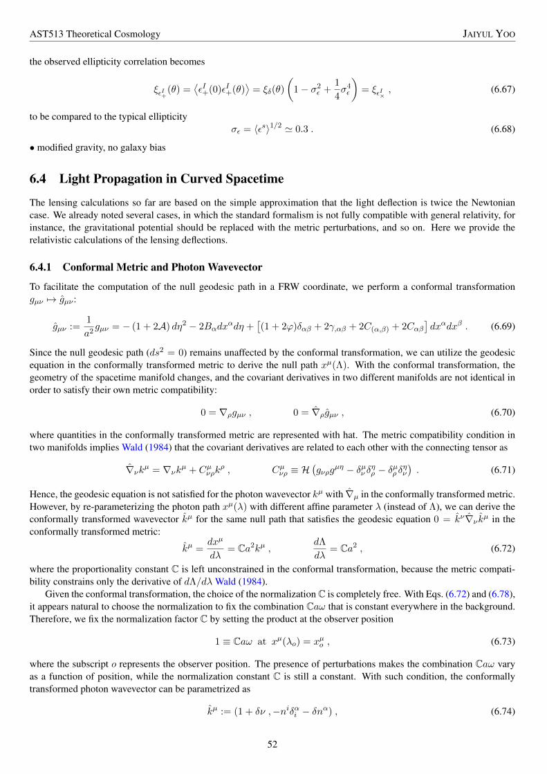
AST513 Theoretical Cosmology JAIYUL YOO
the observed ellipticity correlation becomes
ξεI+(θ) =
⟨εI+(0)εI+(θ)
⟩= ξδ(θ)
(1− σ2
ε +1
4σ4ε
)= ξεI×
, (6.67)
to be compared to the typical ellipticityσε = 〈εs〉1/2 ' 0.3 . (6.68)
• modified gravity, no galaxy bias
6.4 Light Propagation in Curved Spacetime
The lensing calculations so far are based on the simple approximation that the light deflection is twice the Newtoniancase. We already noted several cases, in which the standard formalism is not fully compatible with general relativity, forinstance, the gravitational potential should be replaced with the metric perturbations, and so on. Here we provide therelativistic calculations of the lensing deflections.
6.4.1 Conformal Metric and Photon Wavevector
To facilitate the computation of the null geodesic path in a FRW coordinate, we perform a conformal transformationgµν 7→ gµν :
gµν :=1
a2gµν = − (1 + 2A) dη2 − 2Bαdx
αdη +[(1 + 2ϕ)δαβ + 2γ,αβ + 2C(α,β) + 2Cαβ
]dxαdxβ . (6.69)
Since the null geodesic path (ds2 = 0) remains unaffected by the conformal transformation, we can utilize the geodesicequation in the conformally transformed metric to derive the null path xµ(Λ). With the conformal transformation, thegeometry of the spacetime manifold changes, and the covariant derivatives in two different manifolds are not identical inorder to satisfy their own metric compatibility:
0 = ∇ρgµν , 0 = ∇ρgµν , (6.70)
where quantities in the conformally transformed metric are represented with hat. The metric compatibility condition intwo manifolds implies Wald (1984) that the covariant derivatives are related to each other with the connecting tensor as
∇νkµ = ∇νkµ + Cµνρkρ , Cµνρ ≡ H
(gνρg
µη − δµν δηρ − δµρ δην). (6.71)
Hence, the geodesic equation is not satisfied for the photon wavevector kµ with ∇µ in the conformally transformed metric.However, by re-parameterizing the photon path xµ(λ) with different affine parameter λ (instead of Λ), we can derive theconformally transformed wavevector kµ for the same null path that satisfies the geodesic equation 0 = kν∇ν kµ in theconformally transformed metric:
kµ =dxµ
dλ= Ca2kµ ,
dΛ
dλ= Ca2 , (6.72)
where the proportionality constant C is left unconstrained in the conformal transformation, because the metric compati-bility constrains only the derivative of dΛ/dλ Wald (1984).
Given the conformal transformation, the choice of the normalization C is completely free. With Eqs. (6.72) and (6.78),it appears natural to choose the normalization to fix the combination Caω that is constant everywhere in the background.Therefore, we fix the normalization factor C by setting the product at the observer position
1 ≡ Caω at xµ(λo) = xµo , (6.73)
where the subscript o represents the observer position. The presence of perturbations makes the combination Caω varyas a function of position, while the normalization constant C is still a constant. With such condition, the conformallytransformed photon wavevector can be parametrized as
kµ := (1 + δν ,−niδαi − δnα) , (6.74)
52

AST513 Theoretical Cosmology JAIYUL YOO
and the four velocity in the conformally transformed metric is
u = auµ , uµ = gµν uν =
uµa. (6.75)
We define the perturbation ∆ν in the observed frequency in the conformally transformed metric, in terms of the product
Caω = −Ca (uµkµ) = −uµkµ = 1 + δν +A+ (Uα −Bα)nα := 1 + ∆ν . (6.76)
6.4.2 Boundary Condition for Photon Wavevector
The photon wavevector is measured in the observer rest-frame as
ka = eaµkµ = (ω, k) = ω(1 ,−n) , ω = |k| , |n| = 1 , (6.77)
where we expressed the components of the photon wavevector in the observer rest-frame, in terms of the observablequantities: the angular frequency ω = 2πν of the photon and the angular position n of the source. In the observer rest-frame, a set of angles (θ, φ) is assigned to the unit directional vector ni = (sin θ cosφ, sin θ sinφ, cos θ). Using the tetradexpression in Eq. (5.4), we can derive the photon wavevector in a FRW coordinate
kµ = eµaka =
ω
a
[1−A− niδβi (Uβ −Bβ) ,−niδαi + Uα + niδβi
(ϕ δαβ + Gα,β + Cαβ
)+ εαijn
iΩj]. (6.78)
While the null path xµ(Λ) can be parametrized by any affine parameter Λ, we can physically fix the affine parameter Λby demanding that the tangent vector along the path is the photon wavevector,5
kµ(Λ) =dxµ
dΛ, (6.79)
and Eq. (6.78) is satisfied at the observer position as the boundary condition for the photon wavevector. Therefore, theperturbations to the photon wavevector at the observer position are then
δνo = ∆νo −Ao − niδβi (Uβ −Bβ)o = ∆νo −[αχ + V‖ +
d
dλ
(χa
)+Hχ
]o
, (6.80)
δnαo = niδαi ∆νo − Uαo − niδβi
(ϕ δαβ + Gα,β + Cαβ
)o− εαijniΩj
o (6.81)
= niδαi
(∆ν − ϕχ −Hχ
)o− V α
o −Ψαo − Cαβoδ
βi n
i − εαijniΩjo +
(d
dλGα)o
.
6.4.3 Geodesic Equation and Observed Redshift
The photon wavevector in the conformally transformed metric trivially satisfies the geodesic equation in a homogeneousuniverse. In the presence of perturbations, the perturbations (δν, δnα) to the photon wavevector kµ are constrained by thetemporal and the spatial geodesic equations
0 = kν∇ν kη :=d
dλδν + δΓη , 0 = kν∇ν kα := − d
dλδnα + δΓα , (6.82)
where we defined the derivative along the photon path with respect to the affine parameter
d
dλ≡ kµ ∂
∂xµ=
(∂
∂η− nα ∂
∂xα
)+
(δν
∂
∂η− δnα ∂
∂xα
), (6.83)
and the perturbations in the geodesic equations
δΓη ≡ Γηµν kµkν = A′ − 2A,αnα +
(Bα,β + C ′αβ
)nαnβ (6.84)
=d
dλ
[2αχ + 2Hχ+
d
dλ
(χa
)]− (αχ − ϕχ)′ +
(Ψα,β + C ′αβ
)nαnβ ,
δΓα ≡ Γαµν kµkν = A,α −Bα′ −
(Bβ
,α −Bα,β + 2Cα′β
)nβ +
(2Cαβ,γ − Cβγ,α
)nβnγ (6.85)
= (αχ − ϕχ),α −Ψβ,αnβ − Cβγ,αnβnγ −
d
dλ
(2ϕχn
α + Ψα + 2Cαβ nβ + 2Hχnα
)+
d2
dλ2Gα .
5Note that not all tangent vectors of a given path correspond to the photon wavevector. So, the condition that the tangent vector in Eq. (6.79) isthe photon wavevector completely fixes the parametrization of the path.
53

AST513 Theoretical Cosmology JAIYUL YOO
Note that we already chose a rectangular coordinate for our flat FRW coordinate, in which the Christoffel symbols vanishin the background. In addition to the geodesic equation, the perturbations to the photon wavevector are subject to the nullcondition 0 = kµkµ:
nαδnα = δν +A−B‖ − C‖ , C‖ := Cαβnαnβ . (6.86)
With the explicit expressions of the geodesic equations, we integrate them over the affine parameter to obtain the pertur-bations (δν, δnα)λ along the photon path xµλ:
δνλ − δνo = −∫ λ
0dλ′ δΓη (6.87)
= −[2αχ + 2Hχ+
d
dλ
(χa
)]λλo
+
∫ λ
λo
dλ′[(αχ − ϕχ)′ −
(Ψα,β + C ′αβ
)nαnβ
]= −
[2αχ −Ψ‖ + 2Hχ+
d
dλ
(χa
)]λλo
−∫ rλ
0dr(αχ − ϕχ −Ψ‖ − C‖
)′,
and
δnαλ − δnαo =
∫ λ
0dλ′ δΓα = −
[2ϕχn
α + Ψα + 2Cαβ nβ + 2Hχnα − d
dλGα]λλo
−∫ rλ
0dr[(αχ − ϕχ),α −Ψβ
,αnβ − Cβγ,αnβnγ], (6.88)
where the quantities in the square bracket are evaluated at the source and the observer positions parametrized by λ and λo.Note that the derivative dλ along the photon path was considered only at the background level and we replaced it withthe integration over the comoving distance dr, all of which are valid only when the integrands are at the linear order inperturbations. The perturbations (δν, δnα)o at the observer position are fixed in Eq. (6.80) as the boundary condition.
Before we proceed to obtain the source position xµs by integrating the geodesic equations once more over the affineparameter, we derive the expression for the observed redshift. The light emitted in the rest-frame of the source travelsacross the Universe, and its wavelength is stretched due to the expansion. With reference to the rest-frame wavelengthor the emission frequency ωs in the source rest-frame, the observed redshift z is constructed by using the observedfrequency ωo at the observer as
1 + z :=ωsωo
=k0s
k0o
=(uµk
µ)s(uµkµ)o
=aoas
(1 + ∆νs − ∆νo
):=
1 + δz
as, (6.89)
where we used Eq. (6.76) and we defined the perturbation δz in the observed redshift. In addition to the cosmic expansion,the perturbations along the light propagation affect the observed redshift, and the perturbation δz in the observed redshiftcaptures such effects of inhomogeneities. Noting that the observer time-coordinate is ηo = ηo + δηo and the expressionfor the perturbation δν is Eq. (6.87), we can derive the expression for δz as
δz ≡ Hoδηo + ∆νs − ∆νo = −Hχ+ (Hδη +Hχ)o +[V‖ − αχ + Ψ‖
]λsλo−∫ rs
0dr(αχ − ϕχ −Ψ‖ − C‖
)′. (6.90)
The photon wavelength (hence the observed redshift) is affected by the peculiar velocity and the gravitational redshift ofthe observer and the source positions. The latter is called the Sachs-Wolfe effect. Furthermore, the time evolution of thegravitational potential along the line-of-sight also gives rise to the integrated Sachs-Wolfe effect.
6.4.4 Source Position in FRW Coordinates
The photon path is a straight line in a homogeneous universe, and the inhomogeneities in the real universe deflect thephoton path from a straight line. We will begin the calculations by considering a homogeneous universe first and therebyobtaining the relation to the affine parameter set by our normalization condition in Eq. (6.73). Any position xµλ along thephoton path will be marked by the affine parameter λ, and we will use bar to indicate that the position is derived in ahomogeneous universe:
xµλ − xµo =
∫ λ
0dλ′ ˆkµλ′ = (λ ,−λ nα) , (6.91)
54

AST513 Theoretical Cosmology JAIYUL YOO
where we set to zero the affine parameter at the observer λo = 0 and the position of the observer in a homogeneousuniverse is uniquely set xµo := (ηo, 0). As a coordinate in the world-line manifold, the affine parameter is defined by theabove equation as
λ := ηλ − ηo = −rλ , (6.92)
hence the spatial position becomesxαλ = −λ nα = rλn
α . (6.93)
The observed redshift is the only way we can assign a physically meaningful distance to cosmological objects. Since thecomoving distance r is often defined in terms of a redshift parameter z, we define the affine parameter λz and the timecoordinate ηz of the source in the background in terms of the observed redshift z as
λz := ηz − ηo = −rz , 1 + z =a(ηo)
a(ηz), rz =
∫ z
0
dz′
H(z′). (6.94)
We have used bar for the position xµλ = (η, xα)λ along the photon path to indicate that this position is evaluated in ahomogeneous universe, given the observed angle ni in the observer rest-frame.
With (δν, δnα) in Eqs. (6.87) and (6.88), we can derive the expression for any position xµλ along the path by integratingthe perturbations over the affine parameter. First, we integrate the temporal part of the photon wavevector:
δηλ − δηo = λ(
∆ν + αχ − V‖ −Ψ‖ +Hχ)o−(χa
)+(χa
)o
+
∫ rλ
0dr(2αχ + 2Hχ−Ψ‖
)+
∫ rλ
0dr (rλ − r)
(αχ − ϕχ −Ψ‖ − C‖
)′, (6.95)
such that the time coordinate of the source position is ηs = ηs + δηs. However, since the distance is more physicallyrelated to the observed redshift, we first relate the affine parameter λs at the source position to the observed redshift as
λs = ηs − ηo ≡ λz + ∆λs , (6.96)
where we defined the residual deviation ∆λs of the affine parameter λs from λz . Then the time-coordinate of the sourceposition becomes
ηs = ηz + δηs + ∆λs ≡ ηz + ∆ηs , (6.97)
and the definition of the perturbation δz in Eq. (6.89) yields
∆ηs =δz
H. (6.98)
Next, we integrate the spatial part of the photon wavevector to obtain the source position in a FRW coordinate. Asmentioned, it proves convenient to express the source position xµs around the position xµz inferred from the observedredshift and angle. Having computed the time distortion ∆ηs in Eq. (6.98), we will compute the spatial distortion ∆xαs ofthe source position as
xαs := xαz + ∆xαs = δxαo − λsnα −∫ λs
0dλ δnα = xαz + δxαo −∆λsn
α +
∫ rz
0dr δnα . (6.99)
Given the privileged direction nα, we decompose the spatial distortion into the radial δr distortion and the transversedistortion δxα⊥ as
∆xαs ≡ δr nα + ∆xα⊥ , δr = nα∆xαs , 0 = nα∆xα⊥ , (6.100)
where the radial distortion is
δr = nαδxαo −∆λs −
[χa
+ G‖]zo
+
∫ rz
0dr(δν + αχ − ϕχ −Ψ‖ − C‖
)= (χo + δηo)−
δzχHz
+
∫ rz
0dr(αχ − ϕχ −Ψ‖ − C‖
)+ nα (δxα + Gα)o − nαG
αs , (6.101)
where we used the null condition in Eq. (6.86) and the distortion in the time coordinate in Eq. (6.98). The expression for δris arranged in terms of gauge-invariant variables, isolating the gauge-dependent term nαGαs , such that δr = δr + nαLαs .
55

AST513 Theoretical Cosmology JAIYUL YOO
Being the spatial distortion, the radial distortion δr depends on the spatial position xαo of the observer and hence thecoordinate shift δxαo , but again it is independent of the rotation Ωi
o of the spatial tetrad vectors (same for the distortion ∆ηsin the time coordinate).
For the transverse components ∆xα⊥ of the spatial distortions, we have to integrate δnαλ in Eq. (6.88) over the affineparameter as∫ rz
0dr δnαλ = rz
[δnα + 2Hχnα − d
dλGα + 2ϕχn
α + Ψα + 2Cαβ nβ
]o
− Gαs + Gαo (6.102)
−∫ rz
0dr[2Hχnα + 2ϕχn
α + Ψα + 2Cαβ nβ]−∫ rz
0dr(rz − r)
[(αχ − ϕχ),α −Ψβ
,αnβ − Cβγ,αnβnγ].
Further splitting the transverse distortion by using θα and φα
∆xα⊥ ≡ rz (δθ, sin θ δφ) , rzδθ = θα∆xαs , rz sin θ δφ = φα∆xαs , (6.103)
we derive the angular distortions as
rzδθ = rzθα
[−V α + Cαβ n
β − εαijniΩj]o−∫ rz
0dr θα
[Ψα + 2Cαβ n
β]
(6.104)
−∫ rz
0dr(rz − r)θα
[(αχ − ϕχ),α −Ψβ
,αnβ − Cβγ,αnβnγ]
+ θα (δxα + Gα)o − θαGαs ,
where we used δnαo in Eq. (6.80). For the azimuthal distortion sin θ δφ, the above equation can be used with θα replacedwith φα. The derivative in the second integration in Eq. (6.104) cannot be pulled out for the vector and the tensorperturbations, because it is the derivative with respect to the observed angle due to θα:
Ψβ,αθαnβ =
1
r
(∂
∂θΨ‖ −Ψαθ
α
), Cβγ,αθ
αnβnγ =1
r
(∂
∂θC‖ − 2Cαβn
αθβ). (6.105)
With such expressions, we can further simplify the angular distortions as
δθ = θα
[−V α + Cαβ n
β − εαijniΩj]o−∫ rz
0
dr
rθα
[Ψα + 2Cαβ n
β]
(6.106)
−∫ rz
0dr
(rz − rrz r
)∂
∂θ
(αχ − ϕχ −Ψ‖ − C‖
)+θαrz
[(δxα + Gα)o − Gαs ] .
This equation should be compared to Eq. (6.11) in the standard lensing formalism. We readily notice the incompletenessof the formula in the standard formalism.
In summary, the source position xµs , given the observed redshift z and the observed angle ni, is expressed as the sumof the position xµs inferred from these observables and the deviation ∆xµs around it:
xµs (z, θ, φ) = (ηz + ∆ηs, rz + δr, θ + δθ, φ+ δφ) = xµz + ∆xµs , xµz =(ηz, rzn
i), (6.107)
where the components of the source position is written in a spherical coordinate. These angular distortions of the sourceposition replace the lensing potential in the lens equation as
s = n+ (δθ, δφ) . (6.108)
Given the angular distortion (δθ, δφ) in Eq. (6.104), it is straightforward to compute the lensing convergence:
−2κ ≡ −2
(1− 1
2Tr D
)=
(cot θ +
∂
∂θ
)δθ +
∂
∂φδφ (6.109)
= (2V‖ − 3C‖)o +
∫ rz
0
dr
r
(2nα − ∇α
)(Ψα + 2Cαβ n
β)− 2nα
rz(Gα + δxα)o +
2nαGα
rz
−∫ rz
0dr
(rz − rrz r
)∇2(αχ − ϕχ −Ψ‖ − C‖
)− 1
rz∇αGα ,
where all the terms are arranged in terms of gauge-invariant variables except two terms multiplied with Gα, such that thegravitational lensing convergence gauge-transforms as
κ = κ+nαLα
rz− 1
2rz∇αLα . (6.110)
56

BibliographyJ. M. Bardeen, Phys. Rev. D 22, 1882 (1980).
C.-P. Ma and E. Bertschinger, Astrophys. J. 455, 7 (1995), arXiv:astro-ph/9401007.
D. H. Lyth, Physical Review Letters 78, 1861 (1997), hep-ph/9606387.
R. M. Wald, General relativity (The University of Chicago Press, Chicago, ISBN 0-226-87033-2, 1984).