astronomy and 12 (02.05.2; 02.16.1; 08.09.3; 08.05 ... - … · technique of pade´ approximants as...

arX

iv:a

stro

-ph/

0008

399v

1 2

5 A

ug 2

000

A&A manuscript no.(will be inserted by hand later)

Your thesaurus codes are:12 (02.05.2; 02.16.1; 08.09.3; 08.05.3; 08.12.2; 08.23.1)

ASTRONOMYAND

ASTROPHYSICS

Thermodynamical properties of stellar matter

II. Internal energy, temperature and density exponents,and specific heats for stellar interiors

W. Stolzmann1,2 and T. Blocker3

1 Institut fur Theoretische Physik und Astrophysik, Olshausenstr. 40, D-24098 Kiel, Germany ([email protected])2 Astrophysikalisches Institut Potsdam, An der Sternwarte 16, D-14482 Potsdam, Germany3 Max-Planck-Institut fur Radioastronomie, Auf dem Hugel69, D-53121 Bonn, Germany ([email protected])

Received date; accepted date

Abstract. Starting from the Helmholtz free energy we calcu-late analytically first- and second-order derivatives, as inter-nal energy and specific heats, for the ideal system and the ex-change and correlation interactions covering a broad rangeofdegeneracy and relativity. The complex physics of Coulombinteractions is expressed by Pade Approximants, which reflectthe actual state of our knowledge with high accuracy. We as-sume complete ionization and provide a base system of ther-modynamical functions from which any other thermodynami-cal quantities can be calculated. We chose for the base systemthe free energy, the pressure, the internal energy, the isothermalcompressibility (or density exponent), the coefficient of strain(or temperature exponent), and the isochoric specific heat.Bymeans of the latter potentials entropy, isobaric specific heatand adiabatic temperature gradient can be determined. We givecomparisons with quantities which are composed by numeri-cal second-order derivatives of the free energy and show thatnumerical derivatives of the free energy as calculated, forin-stance, from EOS tables, may produce discontinuities for astro-physically relevant quantities as, e.g., the adiabatic temperaturegradient. Adiabatic temperature gradients are shown for differ-ent chemical compositions (hydrogen, helium, carbon). Finallythe used formalism of Pade Approximants allows immediateincorporation of recent results from many particle statistics.

Key words: Equation of state – Plasmas – Stars: interiors –Stars: evolution – Stars: low-mass, brown dwarfs – Stars: whitedwarfs

1. Introduction

For an accurate modelling of stellar objects we have to computea complete set of thermodynamical quantities which meets thephysical conditions of various evolutionary stages. Basedonthe framework presented in Stolzmann & Blocker (1996a, here-after paper I) we derive further thermodynamical potentials in

Send offprint requests to: W. Stolzmann

order to provide a base system from whichany other thermo-dynamical quantity can be calculated. Such a system requiressix quantities consisting of the Helmholtz free energy, twoofits single derivatives, one of its second mixed derivatives, andtwo of its second pure derivatives with respect to temperatureand density (see e.g. Dappen et al. 1988). We complement theHelmholtz free energy with the pressure and the internal en-ergy, with the isochoric specific heat, and with the temperatureand density exponents in the equation of state (EOS),χT andχρ. This paper will be devoted to the ideal, exchange and corre-lation contributions according to the expansions given in paperI, viz. for case a: weak relativity and arbitrary degeneracy, andcase b: strong degeneracy and arbitrary relativity. These casescover a large area in the density-temperature plane. The cor-relations between the charged particles are formulated by thetechnique of Pade Approximants as in paper I. Here we giveimproved versions of our earlier applied Pade Approximants.In particular we have rearranged terms of the quantum virialfunction.Explicit expressions for the Helmholtz free energy and thepressure have already been derived in paper I for idealityas well as for exchange and correlation interaction. This pa-per aims at providing analytical formulae with high accuracywhich supply quick computing with reliable accuracy in prac-tical applications. Furthermore the expressions of the thermo-dynamical functions given here can be easily included as a partof the thermodynamical description of arbitrary degree of ion-ization.This paper is organized as follows. In Sect. 2 we list the setof thermodynamical potentials to be considered. Sect. 3 givesa brief overview of the concept for the calculation of the EOSterms. Sect. 4 deals with the detailed determination of the ideal,exchange and correlation parts for the EOS. Numerical resultsand comparisons are presented in Sect. 5, and a summary isgiven in Sect. 6.

http://arxiv.org/abs/astro-ph/0008399v1

2 W. Stolzmann and T. Blocker: Thermodynamical propertiesof stellar matter

2. Thermodynamical relations and identities

We summarize briefly some well-known standard relations,which are frequently used to provide the thermodynamics forastrophysical applications.We have to determine the first and second-order quantitieswhich are related by the ratioCP/CV of isochoric to isobaricspecific heat:

γ =CP

CV

= 1 +V

KT

λ2PCVT

, (1)

The (isobaric) thermal expansion coefficientλP can be ex-pressed by

λP =KT

VCVTγG = KTΦS , (2)

with γG being the Gruneisen coefficient

γG =PV

CVTχT . (3)

ΦS is the coefficient of strain

ΦS = PχT , (4)

andKT is the isothermal compressibility

1

KT

= Pχρ . (5)

The so-called temperature and density exponents in the equa-tion of state (Cox & Giuli 1968) are defined by

χT =

(

∂ lnP

∂ lnT

)

ρ

=T

P

(

∂P

∂T

)

V

(6)

χρ =

(

∂ lnP

∂ ln ρ

)

T

= −VP

(

∂P

∂V

)

T

. (7)

The adiabatic temperature gradient defined by∇ad =(∂ lnT/∂ lnP )S (S denotes the entropy) can be expressed by

∇ad =PV

CPTλP =

PV

CPT

χT

χρ. (8)

Another possibility to calculate the adiabatic gradient isgivenby the three adiabatic exponentsΓ1, Γ2, andΓ3 (Cox & Giuli1968, Rogers et al. 1996)

∇ad =Γ2 − 1

Γ2

=Γ3 − 1

Γ1

, (9)

which can be obtained by

Γ1 =γ

PKT

, Γ2 =γ

γ − PKTγG, Γ3 = 1 + γG . (10)

In order to calculate the quantities given by Eqs. (1)-(10) westart with the Helmholtz free energyF (V, T,N) and determineby means of standard thermodynamic relations the Gibbs en-ergy,

G = N

(

∂F

∂N

)

T,V

, (11)

the pressure,

PV = G− F , (12)

and the internal energy,

U = F − T

(

∂F

∂T

)

V,N

, (13)

leading to the entropyS according to

TS = U − F (14)

and to the isochoric specific heat via

CV =

(

∂U

∂T

)

V,N

= −T(

∂2F

∂T 2

)

V,N

. (15)

Moreover, we have to calculate the coefficient of strain and theinverse compressibility (bulk modulus) by means of Eqs. (4)-(7).

3. Theoretical model

As in paper I we start with the Helmholtz free energyF of afully ionized plasma consisting of ideal and Coulomb interac-tion parts

F (T, V,Na) =∑

a

F ida + F coul , (16)

where the Coulomb term contains the following parts:

F coul = F xee + F c

ee + F cii + F cq

ii + F cie , (17)

with x and c marking the exchange and correlation contribu-tions and cq the quantum correction term. The pairsab denotethe interaction between particles of speciesa andb (electrons,ions), respectively.

For convenience we introduce dimensionless thermody-namical potentials defined by

f =F

NkT, g =

G

NkT, p =

P

nkT, u =

U

NkT(18)

s =S

Nk,

1

kT=

1

KT nkT, φS =

ΦS

nkT, cV =

CV

Nk(19)

wheren = N/V refers to the total particle number density ofthe ionsor the electrons, andk denotes the Boltzmann con-stant. Eq. (16), or correspondingly the potentials summarizedby Eq. (18) and Eq. (19), can be written by

Σ = NekT[

σide + σx

ee + σcee

]

+

NikT[

σidi + σc

ii + σcqii + σc

ie

]

(20)

whereΣ = {F, G, P · V, U, S · T, V/KT, ΦS · V, CV · T }and σ = {f, g, p, u, s, 1/kT, φS, cV} symbolize the variousthermodynamic functions defined in the previous section.

W. Stolzmann and T. Blocker: Thermodynamical properties of stellar matter 3

4. Thermodynamical potentials

This section deals in detail with the calculation of the poten-tials listed in Eq. (20). By introducing definitions and for thesake of the integrity we repeat here few expressions concerningHelmholtz free energy and pressure, which are already giveninpaper I.

4.1. Ideality

The ideality of the nonrelativistic and nondegenerate ionsis described by the well-known classical expressions for theHelmholtz free energy

f idi =

[

ln(

niΛ3i

)

− 1]

. (21)

The thermal de Broglie wavelength for particles of speciesa isΛa = 2πh/

√2maπkT . In the classical description we get for

the pressure, the compressibilty, and the coefficient of strain

pidi =1

kidT,i= φidS,i = 1 , (22)

and for the internal energy and the isochoric specific heat

uidi = cidV,i =3

2. (23)

The ideal pressure of the electrons at any relativity and de-generacy (Chandrasekhar 1939, Cox & Giuli 1968) can be cal-culated by

pide =2

neΛ3e

[

J3/2(ψ, λ) +5

4λJ5/2(ψ, λ)

]

, (24)

with the correponding particle number density

ne =2

Λ3e

[

J1/2(ψ, λ) +3

2λJ3/2(ψ, λ)

]

. (25)

The thermodynamical potentials of the electrons are character-ized by the relativistic Fermi-Dirac integralsJν(ψ, λ), whichdepend on the degeneracy (ψ) and the relativity (λ) parameters

ψ =µ

kT, λ =

kT

mc2. (26)

Generally, the degeneracy parameterψ in (26) is a function ofthe density and temperature defined by Eq. (25). In order toevaluate the free energy

f ide = ψ − pide (27)

we have to determineψ explicitly from Eq. (25) by an inversionprocedure which has to be performed numerically. Note, thatψin (26) is identical with the ideal contribution ofg in (18), i.e.ψ = gide . Lamb (1974) and Lamb & Van Horn (1975) evaluatedthe thermodynamical potentials applying the parametrizationsof Eggleton et al. (1973) for the relativistic Fermi-Dirac inte-grals. Johns et al. (1996) improved the accuracy of the poly-nomials given by Eggleton et al. (1973). Straniero (1988) cal-culated the complete set of thermodynamical functions based

on the expressions given in Eqs. (24)-(27) by numerical inte-grations to determine the adiabatic temperature gradient.Re-cently, Blinnikov et al. (1996) and Miralles & Van Riper (1996)presented parametrizations and used various approximations toevaluate the fully relativistic ideality for the set of thermody-namical potentials, which are listed in Sect. 3. However, allcalculational schemes are characterized by an immense effortin order to determine temperature- and density derivationsevenfor asymptotic regions. For details, see e.g. Miralles & VanRiper (1996).

We pursue to include relativistic effects over a broad re-gion of astrophysically relevant densities and temperatures forideality and exchange. Furthermore we evaluate the set of ther-modynamical potentials analytically avoiding the well-knownnoise problems of second-order quantities apparent in purelynumerical approaches.This can be realized by introducing two approximations:a) arbitrary degeneracy, but weak relativity (case a) andb) arbitrary relativity, but strong degeneracy (case b)A numerical study on the density-temperature validity regionof these approximations was carried out in paper I. Note, thatcase a, based onλ-expansions∼ O(λ4), is limited to T <∼2 · 109K andρ <∼ 106g/cm3, whereascase b, based on1/ψ-Sommerfeld-Chandrasekhar expansions∼ O(ψ−6) holds forψ >∼ 5 (see Fig. 1 in paper I).

Carrying out the expansions (∼ O(λ4)) in case a we get forEqs. (24) and (25)

pide =I3/2(ψ)

I1/2(ψ)

Ua(ψ, λ)

V a(ψ, λ)(28)

ne =2

Λ3e

I1/2(ψ) Va(ψ, λ) , (29)

with the abbreviationsUa andV a (not to be confused with theinternal energy or the volume)

Ua = 1 +15

8λI5/2

I3/2

[

1 +7

16λI7/2

I5/2

(

1− 3

8λI9/2

I7/2

)]

(30)

and

V a = 1 +15

8λI3/2I1/2

[

1 +7

16λI5/2I3/2

(

1− 3

8λI7/2I5/2

)]

(31)

taking into account relativistic corrections.Iν = Iν(ψ) =∫∞0dz zν(ez−ψ+1)−1/Γ(ν+1) are the nonrelativistic Fermi-

Dirac integrals considered by parametrizations and expansions(see e.g. paper I).

For the Helmholtz free energy in Eq. (27) we have per-formed the inversionψ = ψ(ne, T ) analytically (see paper I).Using the Maxwell relation Eq. (13) and Eqs. (4)-(7) we obtainfor the internal energy, compressibility, and coefficient of strain

uide =3

2pide +

15

8λI5/2

I1/2

Uaλ

V a(32)

1

kidT,e=

I1/2

I−1/2

V a

V aψ

(33)


φidS,e = uide + pide − 3

2

I1/2

I−1/2

[

V a

V aψ

+5

4λI3/2

I1/2

V aλ

V aψ

]

. (34)

Obviously, Eq. (32) results forλ → 0 in the well-known non-relativistic relationuid = 3

2pid. Calculating the derivatives of

the free energy with respect to the temperature in order to getthe isochoric specific heat (Eq. 15) we have to execute ex-plicitely

CV = −T[

∂2F

∂T 2+ 2

dψ

dT

∂2F

∂ψ∂T

+

(

dψ

dT

)2∂2F

∂ψ2+

d2ψ

dT 2

∂F

∂ψ

]

V,Na

.(35)

The temperature derivatives ofψ at constantV andNe must becalculated from Eq. (29) giving

Tdψ

dT= −3

2

I1/2

I−1/2

[

V a

V aψ

+5

4λI3/2

I1/2

V aλ

V aψ

]

, (36)

T 2 d2ψ

dT 2=

15

4

I1/2

I−1/2

V a

V aψ

−[

3

5

I1/2

I−1/2

V a

V aψ

I−3/2

I−1/2

V aψψ

V aψ

+3

4λ

(

I1/2

I−1/2

V aλψ

V aψ

− I3/2

I−1/2

V aλ

V aψ

I−3/2

I−1/2

V aψψ

V aψ

)

+15

8λ2

I3/2

I−1/2

V aλ

V a

(

I1/2

I−1/2

V aλψ

V aψ

−1

2

I3/2

I1/2

V aλ

V aψ

I−3/2

I−1/2

V aψψ

V aψ

− 7

30

I5/2

I3/2

V aλλ

V aλ

)]

.(37)

Finally, Eq. (35) divided byNek yields the ideal part of theelectronic specific heat

cidV,e =15

4

[

I3/2

I1/2

Ua

V a− 3

5

I1/2

I−1/2

V a

V aψ

]

+75

8λ

[

I5/2I1/2

Uaλ

V a− 3

5

I3/2I−1/2

V aλ

V aψ

]

+105

64λ2

[

I7/2

I1/2

Uaλλ

V a− 15

7

I3/2

I−1/2

V aλ

V aψ

I3/2

I1/2

V aλ

V a

]

,(38)

where the abbreviations are given by

Uaλ = 1 +

7

8λI7/2

I5/2

(

1− 9

16λI9/2

I7/2

)

(39)

Uaλλ = 1− 9

8λI9/2

I7/2(40)

V aλ = 1 +

7

8λI5/2

I3/2

(

1− 9

16λI7/2

I5/2

)

(41)

V aλλ = 1− 9

16λI7/2

I5/2(42)

V aψ = 1 +

15

8λI1/2

I−1/2

[

1 +7

16λI3/2

I1/2

(

1− 3

8λI5/2

I3/2

)]

(43)

V aψψ = 1 +

15

8λI−1/2

I−3/2

[

1 +7

16λI1/2

I1/2

(

1− 3

8λI3/2

I1/2

)]

(44)

V aψλ = 1 +

7

8λI3/2

I1/2

(

1− 9

16λI5/2

I3/2

)

. (45)

From these relations we can read off immediately variousasymptotics. The nonrelativistic (λ ≪ 1) and nondegeneratelimit (ψ ≪ −1) of Eq. (38) results to the well-known classicalvalue

cidV,e =3

2. (46)

Furthermore in the nonrelativistic limit and at arbitrary degen-eracy the comparison of Eqs. (34) and (38) yields

φidS,e =2

3cidV,e . (47)

Case b describes the regime where the Sommerfeld-Chandrasekhar expansion (Chandrasekhar 1939, Cox & Giuli1968) becomes valid. The degeneracy parameterψ is relatedfor the strong-degenerate limit by

ψλ =√

1 + α2 − 1 , (48)

whereα = pF/mc is the fraction of the Fermi- to the rel-ativistic momentum. The Sommerfeld-Chandrasekhar expan-sion with∼ O(ψ−6) provides (Cox & Giuli 1968)

pide =1

4λ

Ub(ψ, λ)

V b(ψ, λ), (49)

ne =2

Λ3e

√

2

π

α3

3λ3/2V b(ψ, λ) =

(mc

h

)3 α3

3π2V b(ψ, λ) ,(50)

with the abbreviations

Ub =√

1 + α2

[

1− 3

2α2+

3

2α3√1 + α2

ln(

α+√

1 + α2

)

+2π2λ2

α2

(

1− 7

60

π2λ2

α4

(

1− 2α2)

)]

(51)

and

V b = 1 +π2λ2

2α4

(

1 + 2α2 +7

20

π2λ2

α4

)

. (52)

For the Helmholtz free energy represented by Eq. (27) the in-versionψ = ψ(ne, T ) for case b is already given by Eq. (48).In order to correct Eq. (48) to the order∼ O(ψ−6) analyti-cal inversions have been performed by Yakovlev & Shalybkov(1989) and paper I.

For the internal energy, compressibility, and coefficient ofstrain we get

uide =1

λ

[

√

1 + α2 − 1 +1

4

(

Ub

V b+Ubλ

V b

)]

(53)


1

kide=

1

λ

[

α2

√1 + α2

(

V b

3V b + V bα

)]

(54)

φide =1

λ

[

1

4

Ubλ

V b− α2

√1 + α2

(

V bλ

3V b + V bα

)]

. (55)

Neglecting the orderψ−6 in Eq. (53) we get the Chandrasekharapproximation for the internal energy (Chandrasekhar 1939,Cox & Giuli 1968, Lamb 1974, Eliezer et al. 1986, Yakovlev& Shalybkov 1989)

uide =1

NekT

mc2

8π2

(mc

h

)3

×[

α√

1 + α2(1 + 2α2)− 8

3α3− ln

(

α+√

1 + α2

)

+4

3

π2λ2

α

(

√

1 + α2(1 + 3α2)− (1 + 2α2))

]

.(56)

The specific heat Eq. (15) can be calculated forcase b via

CV = −T[

∂2F

∂T 2+ 2

dα

dT

∂2F

∂α∂T

+

(

dα

dT

)2∂2F

∂α2+

d2α

dT 2

∂F

∂α

]

V,Na

.(57)

The temperature derivatives ofα at constantV andNe must becalculated from Eq. (50)

T

α

dα

dT= − V b

λ

3V b + V bα

, (58)

T 2

α

d2α

dT 2=

T

α

dα

dT

[

V bλλ

V bλ

+ 2T

α

dα

dT

V bαλ

V bλ

−(

T

α

dα

dT

)2(12V b

V bλ

− V bαα

V bλ

)

]

.(59)

Finally, Eq. (57) divided byNek yields

cidV,e = − 1

λ

{

(

√

1 + α2 − 1) V b

λλ

V b− 1

4

Ubλλ

V b

+2T

α

dα

dT

[

(

√

1 + α2 − 1)

(

3V bλ

V b+V bαλ

V b

)]

−(

T

α

dα

dT

)2 [

6(

√

1 + α2 − 1)

(

1 +V bα

V b+

1

6

V bαα

V b

)

−3Ub

V b+

1

4

Ubαα

V b− α2

(1 + α2)3/2

(

1 + 2(1 + α2)V bα

V b

)]

+T 2

α

d2α

dT 2

[

(

√

1 + α2 − 1)

(

3 +V bα

V b

)]}

. (60)

Here the abbreviations labeled by the superscript b are givenby the simple derivatives withX = {Ub, V b}

Xλ = λ∂

∂λX , Xλλ = λ2

∂2

∂λ2X , (61)

Xα = α∂

∂αX , Xαα = α2 ∂

2

∂α2X , (62)

Xαλ = αλ∂2

∂α∂λX . (63)

Eq. (60) yields by neglecting the orderψ−6 (Chandrasekhar1939, Eliezer et al. 1986, Yakolev & Shalybkov 1989)

cidV,e =π2λ

α2

√

1 + α2 , (64)

which delivers the strong-relativistic (α≫ 1)

cidV,e =π2

ψ(65)

and the nonrelativistic (α≪ 1)

cidV,e =π2

2ψ(66)

limiting laws. Let us remark that both Eqs. (38) and (60) havein the degenerate, weak-relativistic limit a wide overlap,whichwe use to combinecase a andb in order to realize numericalcontinuity (see paper I).

4.2. Exchange

The lowest order exchange (Hartree-Fock) free energy for rel-ativistic electrons is given by

fxee =

e2

πΛ4e

1

nekTJxrel(ψ, λ) , (67)

where Jxrel(ψ, λ) is the relativistic Hartree-Fock integral

(Kovetz et al. 1972, paper I).Theλ-expansion incase a results in

fxee = − e2

kTΛe

Ix(ψ)

I1/2(ψ)

W a(ψ, λ)

V a(ψ, λ), (68)

where

W a = 1− 3

8λI21/2

Ix

[

1 +9

8λI3/2

I1/2

(

1 +11

72λI3/2

I1/2×

(

1− 25

11λI5/2

I3/2

I1/2

I3/2

))]

.(69)

Parametrizations for the nonrelativistic Hartree-Fock integral

Ix(ψ) =

∫ ψ

−∞dψ′ I2−1/2(ψ

′) (70)

are given by Perrot & Dharma-wardana (1984) and Kalitkin &Ritus (1986) (see Stolzmann & Blocker 1996b). Note, that forλ = 0 the following relation holds

Jxrel(ψ, λ = 0) = −2π Ix(ψ) . (71)

The exchange pressurepxee = gxee − fxee is determined via the

exchange Gibbs energy (cf. paper I)

gxee = − e2

kTΛe

I−1/2

W aψ

V aψ

, (72)


where

W aψ = 1− 3

4λI1/2

I−1/2

[

1 +9

16λI1/2

I−1/2

(

1 +I3/2

I1/2

I−1/2

I1/2

− 1

24λI3/2

I1/2

(

1 +25

3

I5/2

I3/2

I−1/2

I1/2

))]

(73)

For the exchange contribution of the internal energy, compress-ibility, and coefficient of strain we get

uxee =3

2pxee −

1

2

e2

kTΛe

Ix

I1/2

W aλ

V a+

15

8λI3/2

I1/2

V aλ

V agxee (74)

1

kxT,ee= − e2

kTΛe

I1/2I−3/2

I−1/2

V a

V aψ

[

2W aψψ

V aψ

−V aψψ

V aψ

W aψ

V aψ

]

(75)

φxS,ee = pxee + uxee +1

2

e2

kTΛe

I−1/2

[

3I1/2

I−1/2

I−3/2

I−1/2×

(

2W aψψ

V aψ

−V aψψ

V aψ

W aψ

V aψ

)(

V a

V aψ

+5

4λI3/2

I1/2

V aλ

V aψ

)

+W aψλ

V aψ

+15

4λI1/2

I−1/2

V aψλ

V aψ

W aψ

V aψ

]

. (76)

Using (35) we obtain for the exchange part of the isochoricspecific heat

cxV,e =e2

kTΛe

[

15

4

[

Ix

I1/2

(

W a

V a− 2

3

W aλ

V a+

1

5

W aλλ

V a

)

+3

5

I1/2I−3/2

I−1/2

V a

V aψ

(

2W aψψ

V aψ

−V aψψ

V aψ

W aψ

V a

)

−I−1/2

(

W aψ

V aψ

− 2

5

W aψλ

V aψ

)]

+75

8λ

[

−I3/2I−1/2

I1/2

V aλ

V a

(

W aψ

V aψ

− 1

5

W aψλ

V aψ

)

+3

5

I3/2I−3/2

I1/2

V aλ

V aψ

(

2W aψψ

V aψ

−V aψψ

V aψ

W aψ

V aψ

)

+3

5I1/2

V aψλ

V aψ

W aψ

V aψ

]

+225

64λ2

[

I23/2I−3/2

I1/2I−1/2

V aλ

V aψ

(

2W aψψ

V a−V aψψ

V aψ

W aψ

V a

)

+ 4I3/2I−3/2

I1/2

(

I1/2I−1/2

V aλ

V aψ

V aψλ

V aψ

− 7

30

I5/2I3/2

V aλλ

V aψ

)]]

(77)

with the relativistic corrections

W aλ = 1 +

3

8λI21/2

Ix

[

1 +27

8λI3/2

I1/2

(

1 +55

216λI3/2

I1/2×

(

1− 25

11

I5/2

I3/2

I1/2

I3/2

))]

(78)

W aλλ = 1 +

1

8λI21/2

Ix

[

1− 27

8λI3/2

I1/2

(

1 +55

72λI3/2

I1/2×

(

1− 25

11

I5/2

I3/2

I1/2

I3/2

))]

(79)

W aψψ = 1− 3

8λI1/2I−1/2

[

1 +I−1/2

I−3/2

I−1/2

I1/2

+9

16λI3/2I1/2

(

1 + 3I−1/2

I−3/2

I1/2I3/2

− 7

9λI−1/2

I−3/2×

(

1 +3

28

I1/2I−1/2

I1/2I3/2

+25

28

I5/2I3/2

I−3/2

I−1/2

))]

(80)

W aψλ = 1 +

3

4λI1/2

I−1/2

[

1 +27

16λI3/2

I1/2

(

1 +I1/2

I−1/2

I1/2

I3/2

−125

216λI5/2

I3/2

(

1 +3

25

I3/2

I5/2

))]

.(81)

The Sommerfeld-Chandrasekhar expansion for the exchangefree energy incase b (Salpeter & Zapolsky 1967, Kovetz etal. 1972, Lamb 1974) delivers for∼ O(ψ−6) (see paper I)

fxee = − e2

kTΛe

3

2α3

1√2πλ

W b(α, λ)

V b(α, λ), (82)

where

W b =3B2

2(1 + α2)− 3αB +

3

2α2 +

1

2α4

+π2λ2

3

[

−0.7046 + 2 ln2α2

λ+ α2 − 3B

α

]

+π4λ4

18

[

1− 11

10α2

(

1 +37

11α2+

63B

11α3

)]

(83)

with B =√1 + α2 ln

(

α+√1 + α2

)

.With the Gibbs energy (see paper I)

gxee = − e2

kTΛe

3

2α3

1√2πλ

W bα

3V b + V bα

(84)

it is possible to provide the exchange pressurepxee = gxee − fxee

again.In a straightforward manner, the exchange contribution for

internal energy, compressibility, and coefficient of strain arerepresented by

uxee =e2

kTΛe

3

2α3

1√2πλ

[

W bλ

V b− W b

λ

V b

+W bα

V b

(

V bλ

3V b + V bα

)]

(85)

1

kxT,ee=

e2

kTΛe

3

2α3

1√2πλ

(

V b

3V b + V bα

)2

×[

W bαα

V b− 6W b

α

3V b + V bα

(

1 +V bα

V b+

1

6

V bαα

V b

)]

(86)


φxS,ee = pxee + uxee − gxee

[

1 +3V b

λ + V bαλ

3V b + V bα

− W bαλ

W bα

− V bλ

3V b + V bα

(

2 +4V b

λ + V bαα

3V b + V bα

− W bαλ

W bα

)]

.(87)

The exchange specific heat can be formulated by

cxV,e = − e2

kTΛe

3

2α3

1√2πλ

[

W bλλ

V b+ 2

T

α

dα

dT

W bαλ

V b

+

(

T

α

dα

dT

)2W bαα

V b+T 2

α

d2α

dT 2

W bα

V b

]

(88)

The temperature derivatives ofα in Eq. (88) are given by (58)and (59). The derivatives ofW with respect toλ andα for theexchange contributions are determined by

W bλ = λ

∂

∂λW b , W b

λλ = λ2∂2

∂λ2W b , (89)

W bα = α

∂

∂αW b , W b

αα = α2 ∂2

∂α2W b , (90)

W bαλ = αλ

∂2

∂α∂λW b . (91)

The adiabatic temperature gradient (8) expressed by our dimen-sionless potentials (18) and (19) is given by

∇ad = pkTφScP

=p

φS(1 − cV

cP) (92)

with the isobaric specific heat

cP = cV + kTφ2S (93)

The Figs. 1 and 2 illustrate the adiabatic temperature gradient(92) of the ideal gas im comparison with a gas where addition-ally the exchange term is taken into account. Note, that the rep-resentation in Figs. 1 and 2 for extremely high densities servesonly to illustrate the asymptotics of the theoretical expressions.Processes relevant to such high densities as, e.g., pycnonuclearreactions or electron captures, are not taken into account.Fig. 1illustrates the course of∇ad for the elements hydrogen, heliumand oxygen along a nonrelativistic and a weak-relativistictem-perature. A comparison with the corresponding data for carbonfrom Lamb (1974) is given in Fig. 2. Note a disagreement forT = 105K. This deviation could be caused by an erroneousconstant for the exchange contribution used by Kovetz et al.(1972) and Lamb (1974) and is discussed in detail in paper I. Anumerical procedure to guarantee a smooth transition betweenthe approximations given bycase a and case b is developedin paper I. The curves as seen in Figs. 1 and 2 show how ex-change effects vanish with increasing temperature. Consideringthe isotherms in the high density region exchange effects arenegligible. Nevertheless Eqs. (82)-(88) guarantee the accurateasymptotics, which is a fundamental problem for the calcula-tion of EOS derivatives for quantities with vanishingly smalltemperature dependence (Miralles & Van Riper 1996).

Fig. 1. Adiabatic temperature gradient∇ad vs. density atT =107K andT = 109K for various elements. The curves refer tothe sum of ideality, exchange and radiation. The presentationtowards extremely high densities serves only to illustratetheasymptotic behaviour of the adiabatic gradient in our model(processes relevant to very high densities as, e.g., pycnonuclearreactions or electron captures, are not considered).

4.3. Correlations

According to Eq. (20) we have to determine the terms labeledby the superscript c, which are based on correlation effects.

Fig. 2. Adiabatic temperature gradient∇ad vs. density for car-bon along various isotherms compared with Lamb (1974) (+ :105K, △ : 106K, • : 107K, ◦ : 108K, ∗ : 109K). The curvesrefer to the sum of ideality, exchange and radiation. The presen-tation towards extremely high densities serves only to illustratethe asymptotic behaviour of the adiabatic gradient in our model(processes relevant to very high densities as, e.g., pycnonuclearreactions or electron captures, are not considered).


As in paper I we aim to present closed-form parametrizationsformed by Pade Approximants to get explicite expressions forthe correlation contributions of the thermodynamical poten-tials. The thermodynamical potentials resulting from the cor-relation contributions are characterized by the electronic andionic Coulomb-coupling parametersΓe = (4πne/3)

1/3e2/kTandΓi = Γe〈Z5/3〉 giving the strength of the Coulomb in-teraction, and by the degeneracy parameterΘ = T/TF =2(4/9π)2/3rs/Γe describing the quantum state of the system.The parameterrs = mee

2/h2(3/4πne)1/3 is the ratio of the

mean interelectronic distance to the (electronic) Bohr-radius.

4.3.1. Electron-electron interaction

The Pade Approximants for free Helmholtz- and Gibbs ener-gies of the nonrelativistic electronic subsystem at arbitrary de-generation and Coulomb coupling have the general structure

f cee = −a0Γ

3/2e − a2Γ

6e [εc(rs, 0) + ∆εc(rs, τ)] /τ

1 + a1Γ3/2e + a2Γ6

e

, (94)

gcee = −s0Γ3/2e − s2Γ

6e [µc(rs, 0) + ∆µc(rs, τ)] /τ

1 + s1Γ3/2e + s2Γ6

e

, (95)

with ground-state energiesεc(rs, 0) andµc(rs, 0) derived byVosko et al. (1980) and low-temperature corrections∆εc(rs, τ)and∆µc(rs, τ), which are given in paper I. The coefficientsread

a0 =1√3f0(Γe) , s0 =

3

2a0 +

1

3Γe

da0dΓe

(96)

f0(Γ) =1

2

(

1

(1 + 0.1088Γe)1/2+

1

(1 + 0.3566Γe)3/2

)

(97)

a1 =3√3

32

√2πτ

[

1 +K∗e

(

√

2/τ)]

, s1 =8

9a1 (98)

a2 = 6τ

r2s, s2 = a2 . (99)

Note that we have modified the coefficientsa1 ands1 as com-pared to paper I by a rearrangement of the quantum virial func-tion (Ebeling et al. 1976)

K∗e (x) = E∗

2 (−x)−8x√π

[

Q∗3(−x)−

1

6ln |x| − C0

]

(100)

In paper I we incorporated forK∗e (x) in Eq. (98) only the first

part of Eq. (100) as proposed by Ebeling (1993). The secondterm was considered by the coefficientc1 of the ion-electroncontribution (see Eq. (85) in paper I). The justification to rear-range these summations over the electrons is the omission ofthe coefficienta3 in Eq. (53) in paper I, which has only beenintroduced to optimize the interpolation. ForE∗

2 andQ∗3 we

derived Pade approximations as given in paper I with improve-ments to achieve higher accuracy.

E∗2 (−x) =

ln 2 + 0.0113x2 + 0.1x5(

2√πx

− 1x2

)

1 + π3/2x/(18 ln 2) + 0.1x5(101)

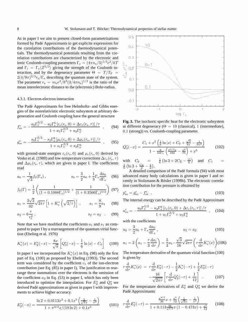
Fig. 3.The isochoric specific heat for the electronic subsystemat different degeneracy (Θ = 10 (classical),1 (intermediate),0.1 (strong)) vs. Coulomb-coupling parameter.

Q∗3(−x) =

C1 + x5(

16ln |x|+ C0 +

√π

8x − 19x2

)

1− 910C1

(

π5/2x192

− x2

75

)

+ x5(102)

with C0 = 16

(

ln 3 + 2CE − 116

)

and C1 =16

(

ln 3 + CE

2− 1

2

)

.A detailed comparison of the Pade formula (94) with most

advanced many body calculations is given in paper I and re-cently in Stolzmann & Rosler (1998b). The electronic correla-tion contribution for the pressure is obtained by

pcee = gcee − f cee , (103)

The internal energy can be described by the Pade Approximant

ucee = −u0Γ3/2e − u2Γ

6e [εc(rs, 0) + ∆εc(rs, τ)] /τ

1 + u1Γ3/2e + u2Γ6

e

, (104)

with the coefficients

u0 =3

2a0 + Γe

da0dΓe

, u2 = a2 (105)

u1 = 2

(

a1 −τ

3

da1dτ

)

=5

3a1−

√3

16

√2πτ

(

τd

dτK∗

e (x)

)

(106)

The temperature derivative of the quantum virial function (100)is given by

τd

dτK∗

e (x) = τd

dτE∗

2 (−τ) −1

2K∗

e (−τ) +1

2E∗

2 (−τ)

− 16√2πτ

[

τd

dτQ∗

3(−τ) +1

12

]

. (107)

For the temperature derivatives ofE∗2 andQ∗

3 we derive thePade Approximants

τd

dτE∗

2 (−τ) =π3/2

36x+ x5

12

(

1√πx

− 1x2

)

1 + 0.113 36π3/2x (1− 0.473x) + x5

12

(108)


τd

dτQ∗

3(−τ) =−π5/2

384x+ 0.1x4.5

(

− 112

+ π1/2

16x − 16x2

)

1 + 38425π5/2x+ 0.1x4.5

.(109)

The correlation contribution1/kcT,ee for the bulk modulus isgiven by

1

kcT,ee=k0Γ

3/2e + k2Γ

6e [pc(rs, 0) (1− 1/kc(rs, 0))] /τ

1 + k1Γ3/2e + k2Γ6

e

(110)


k0 = −3

4a0−

Γe

4

da0dΓe

, k2 = 10a2 , k1 = 30a1 .(111)

The ground-state bulk modulus is given by

1

kc(rs, 0)=

3

0.062181

rs3

d

drspc(rs, 0) . (112)

Using the Monte-Carlo data-fit from Vosko et al. (1980) forpc(rs, 0) (see paper I) we apply

1

kc(rs, 0)=

[

12m1

√rs

1 +m1

√rs

−12m1

√rs +m2rs +

32m3r

3/2s

1 +m1√rs +m2rs +m3r

3/2s

]

(113)

The coefficient of strainφcS,ee can be expressed by

φcS,ee = pcee + ucee

+φ0Γ

3/2e − φ2Γ

6e

[

µc(rs, 0)− 32∆εc(rs, τ)

]

/τ

1 + φ1Γ3/2e + φ2Γ6

e

(114)


φ0 =9

4a0 +

3

4Γe

da0dΓe

, φ2 =1

2a2 , (115)

φ1 =16

9a1 −

2

3τda1dτ

(116)

and for the isochoric specific heatccV,ee the Pade Approximantcan be obtained by

ccV,ee =v0Γ

3/2e − v2Γ

6e

[

2f(rs)Θ2(

1 + 29lnΘ

)]

/τ

1 + v1Γ3/2e + v2Γ6

e

(117)


v0 =3

4

[

a0 +1

4Γe

da0dΓe

]

, v2 = a2 , (118)

v1 =3√3

32

√2πτ

[

1 +7

12

(

1−√2πτ

16K∗

e (−τ))

+1

24(1 + E∗

2 (−τ))−1

2

(

τd

dτE∗

2 (−τ))

−5

6

16√2πτ

(

τd

dτQ∗

3(−τ) +1

12

)]

. (119)

Fig. 3 shows that the electronic correlation part of the isochoricspecific heat can be neglected in the case of strongly degenerateelectrons.

4.3.2. Ion-ion interaction

The classical one-component plasma (OCP) is a thoroughlystudied plasma system and the results are unified in closed-form parametrizations (Hansen 1973, Graboske et al. 1975,Brami et al. 1979, Ebeling & Richert 1985, Ichimaru 1993,Kahlbaum 1996, Chabrier & Potekhin 1998). For the ion-ioncorrelation we modify the Pade Approximants used in paper Iby the new formula (Stolzmann & Blocker 1998, 1999) for thefree energy

f cii = −

b0Γ3/2i

[

1 + b3Γ3/2i F (Γi)

]

+ b2Γ6i εii(Γi)

1− b1Γ3iG(Γi) + b2Γ6

i

, (120)

with F (Γi) = ln Γi +B0 andG(Γi) = ln Γi +B1

B0 =2

3

(

2CE +3

2ln 3− 11

6

)

, (121)

B1 =2

3

(

2CE +1

2ln 3 + 2 ln 2− 17

6

)

− 0.4765 (122)

and the coefficients

b0 =1√3

〈Z2〉3/2〈Z〉1/2〈Z5/3〉3/2 , b1 =

3√3

8b0, (123)

b2 = 100 , b3 =b1√3, (124)

Eq. (120) is based on the classicalΓi < 1 result from Cohen &Murphy (1969) and forΓi

>∼ 1 we take into account the mostrecent Monte-Carlo fit for the free energyεii(Γi) of the liquidOCP from DeWitt & Slattery (1999)

εii(Γi) = 0.899172Γi + 0.274823 lnΓi

−1.864179Γ 0.323064i + 1.4018 . (125)

We remark, that in our notation of Eq. (20) forεii(Γi) we haveto take forΓi

>∼ 178

εii(Γi) = 0.895929Γi − 1.5 lnΓi + 3.9437Γ−1i

+ 1245Γ−2i + 1.1703 (126)

which, with Eq. (21) rewritten by

f idi =

3

2ln

kT

Rydi+ 3 lnΓi − 0.7155, (127)

delivers the thermal (solid phase) energy of the OCP givenby Hansen (1972), Pollock & Hansen (1973), Slattery et al.(1980), and Stringfellow et al. (1990). The quantityRydi =AZ4mp/meRyd denotes the ionic Rydberg energy with the(electronic) Rydberg unitRyd = mee

4/2h2.The free Gibbs energygcii and the isochoric specific heat

ccV,ii are expressed by the Pade Approximants

gcii = −32b0Γ

3/2i

[

1 + 43b3Γ

3/2i

(

F (Γi) +16

)

]

+ b2Γ6i µii(Γi)

1− 53b1Γ3

i

(

G(Γi) +215

)

[

1 + 34Γ3/2i

]

+ b2Γ6i

(128)

10 W. Stolzmann and T. Blocker: Thermodynamical properties of stellar matter

Fig. 4.The compressibility for the ionic subsystem vs. couplingparameterΓi. The solid line represents the correlation contri-bution (133) and the dashed line refers to the parametrizationfrom Hansen (1973).

ccV,ii =

34b0Γ

3/2i

[

1 + 8b3Γ3/2i

(

F (Γi) +56

)

]

+ 6b2Γ6i ii(Γi)

1− 7b1Γ3i

(

G(Γi) +3263

)

+ 6b2Γ6i

(129)

with

µii(Γi) = εii(Γi)+1

3Γi

dεii(Γi)

dΓi

, ii(Γi) = Γ2i

d2εii(Γi)

dΓ2i

.(130)

The pressure, internal energy, isothermal compressibility, andcoefficient of strain (Hansen 1973, Stolzmann & Blocker 1999)are calculated by

pcii = gcii − f cii , (131)

ucii = 3 pcii , (132)

1

kcT,ii= −1

9ccV,ii +

4

9ucii , (133)

φcS,ii =1

3ccV,ii . (134)

Fig. 4 compares our Pade Approximants of the isothermal com-pressibility with the fit formulae from Hansen (1973). Furthercomparisons between different interpolation formulae fortheclassically ionic subsystem, e.g. from Hansen (1973), Ichimaru(1994), Kahlbaum (1996), Chabrier & Potekhin (1998) can befound in Stolzmann & Blocker (1999).

Ionic quantum effects, which were included approximatelyin our earlier Pade Approximants for the ionic subsystem (seepaper I) will be considered separately in the following section.

4.3.3. Ionic quantum effects

The classical description for the subsystem of ionic OCP be-comes inaccurate in the region of high densities at moderate

Fig. 5. The free energy contribution of the ionic quantum cor-rections for carbon atT = 106K vs. ionic quantum param-eter (Eq. 135). The solid line represents Nagara et al. (1987)(Eq. 137) (shown only within its validity regime), the dashedline refers to Chabrier et al. (1992), and the dashed-dottedlineto Iyetomi et al. (1993). The curve labeled by WK refers tothe first order in the Wigner-Kirkwood expansion and HV toHansen & Vieillefosse (1975).

temperatures. A measure for the quantum effects of the ions isthe parameter (weight fractionXi, molecular weightAi, protonmassmp, atomic mass unitmu = 1.66053 · 10−24g)

Θi =hωp

kT=

4√π

kT

(

ρ

mu

me

mp

(

h2

mee2

)3∑

i

Z2iXi

A2i

)1/2

(135)

which is related by

Θi =

√

3

RS

Γi , (136)

and whereasωp denotes the (ionic) plasma frequency andRS = miZ

2e2/h2(3/4πni)1/3 is the ratio of the (ionic)

Wigner-Seitz-radius to the (ionic) Bohr-radius. Quantum cor-rections for a solid OCP over a broad region ofΘi were calcu-lated first by Pollock & Hansen (1973). Chabrier et al. (1992)(see also Chabrier 1993) and Iyetomi et al. (1993) derived anfree energy for a solid OCP model with quantum corrections.Nagara et al. (1987) calculated quantum corrections for thefreeenergy of the OCP valid for fluid and solid phases by a new ex-pansion method. In our model ionic quantum effects accordingto Nagara et al. (1987) as well as Chabrier et al. (1992) will beincluded.

Following paper I, the free energy calculated within the so-called “sixth reduced moment approximation” of Nagara et al.(1987) is given by

f cqii = 3

[

q0(t) + z4q4(t)−3

4

t

Γi

z5q5(t) + z6q6(t)

]

(137)


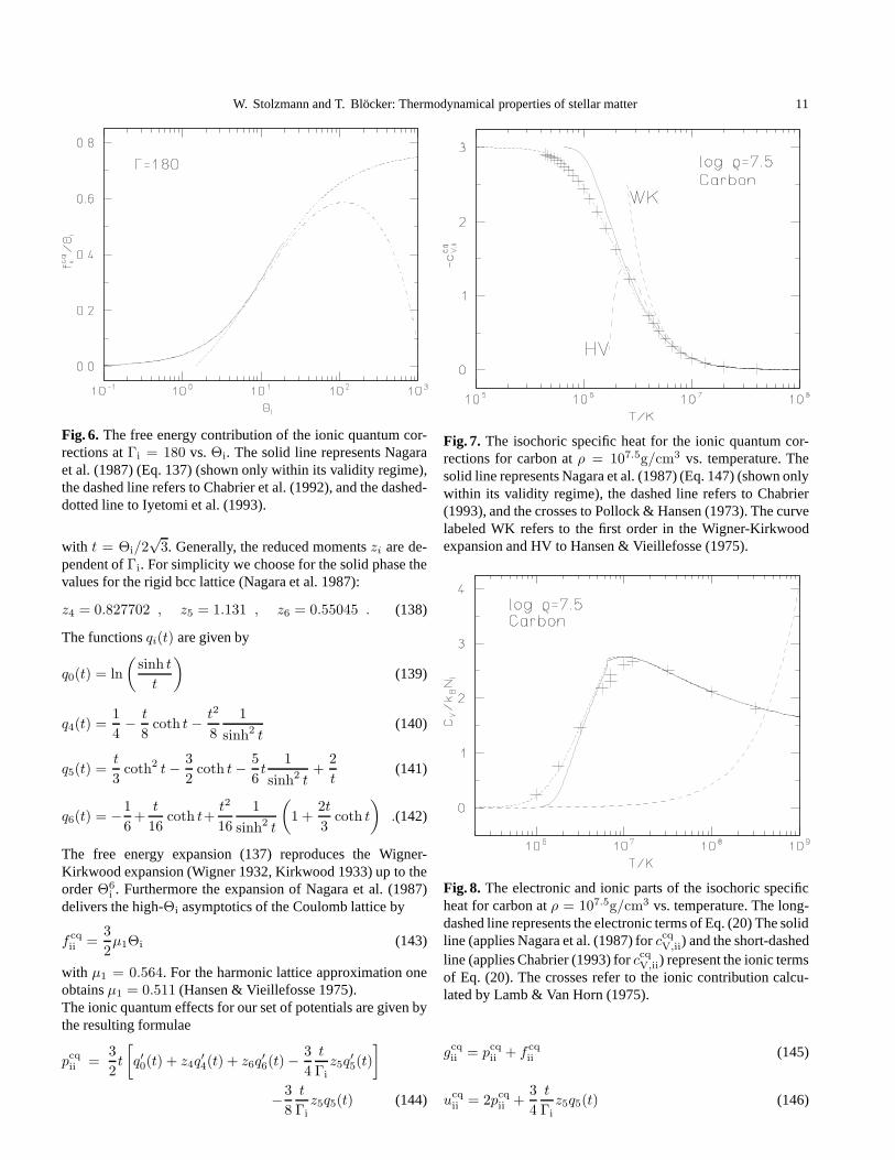
Fig. 6. The free energy contribution of the ionic quantum cor-rections atΓi = 180 vs.Θi. The solid line represents Nagaraet al. (1987) (Eq. 137) (shown only within its validity regime),the dashed line refers to Chabrier et al. (1992), and the dashed-dotted line to Iyetomi et al. (1993).

with t = Θi/2√3. Generally, the reduced momentszi are de-

pendent ofΓi. For simplicity we choose for the solid phase thevalues for the rigid bcc lattice (Nagara et al. 1987):

z4 = 0.827702 , z5 = 1.131 , z6 = 0.55045 . (138)

The functionsqi(t) are given by

q0(t) = ln

(

sinh t

t

)

(139)

q4(t) =1

4− t

8coth t− t2

8

1

sinh2 t(140)

q5(t) =t

3coth2 t− 3

2coth t− 5

6t

1

sinh2 t+

2

t(141)

q6(t) = −1

6+t

16coth t+

t2

16

1

sinh2 t

(

1 +2t

3coth t

)

.(142)

The free energy expansion (137) reproduces the Wigner-Kirkwood expansion (Wigner 1932, Kirkwood 1933) up to theorderΘ6

i . Furthermore the expansion of Nagara et al. (1987)delivers the high-Θi asymptotics of the Coulomb lattice by

f cqii =

3

2µ1Θi (143)

with µ1 = 0.564. For the harmonic lattice approximation oneobtainsµ1 = 0.511 (Hansen & Vieillefosse 1975).The ionic quantum effects for our set of potentials are givenbythe resulting formulae

pcqii =3

2t

[

q′0(t) + z4q′4(t) + z6q

′6(t)−

3

4

t

Γi

z5q′5(t)

]

−3

8

t

Γi

z5q5(t) (144)

Fig. 7. The isochoric specific heat for the ionic quantum cor-rections for carbon atρ = 107.5g/cm3 vs. temperature. Thesolid line represents Nagara et al. (1987) (Eq. 147) (shown onlywithin its validity regime), the dashed line refers to Chabrier(1993), and the crosses to Pollock & Hansen (1973). The curvelabeled WK refers to the first order in the Wigner-Kirkwoodexpansion and HV to Hansen & Vieillefosse (1975).

Fig. 8. The electronic and ionic parts of the isochoric specificheat for carbon atρ = 107.5g/cm3 vs. temperature. The long-dashed line represents the electronic terms of Eq. (20) The solidline (applies Nagara et al. (1987) forccqV,ii) and the short-dashedline (applies Chabrier (1993) forccqV,ii) represent the ionic termsof Eq. (20). The crosses refer to the ionic contribution calcu-lated by Lamb & Van Horn (1975).

gcqii = pcqii + f cqii (145)

ucqii = 2pcqii +3

4

t

Γi

z5q5(t) (146)


ccqV,ii = −3t2[

q′′0 (t) + z4q′′4 (t)−

3

4

t

Γi

z5q′′5 (t) + z6q

′′6 (t)

]

(147)

1

kcqT,ii=

1

4

[

3ucqii − ccqV,ii −3

4

t

Γi

z5

(

7

3q5(t) + 2tq′5(t)

)]

(148)

φcqS,ii =1

2

[

ccqV,ii −3

4

t

Γi

z5

(

q5(t)− tq′5(t)

)]

(149)

The functionsq′i(t) andq′′i (t) are first and second derivativesof the functionsqi(t) with respect tot.

Although the expansion of Nagara et al. (1987) can be ap-plied to estimate quantum effects for fluid ionic phases as wellas for solid phases this expansion is restricted toΘi

<∼ 17,which is equivalent toΓi

<∼ 4 · 103(AZ4/(T/K))1/3 or toρ <∼ 5 · 10−6(T/K))2(A/Z)2 for the density-temperatureregime. ForΓi ≈ Γm

>∼ 180 it is convenient to use the quantumcrystal models from Iyetomi et al. (1993) or from Chabrier etal. (1992), which are applicable for a wide region ofΘi.If we extract the ionic quantum corrections for the free energyof a crystal from Chabrier et al. (1992) one obtains (Stolzmann& Blocker 1994)

f cqii = −2

3D3(αΘi) + 2 ln

[

1− e−αΘi

]

+ ln[

1− e−γΘi

]

+βΘi − 3 ln (δΘi) (150)

with (Chabrier 1993)

α = 0.399 , γ = 0.899 , β = 0.767 . (151)

The last term in (150) withδ = 0.4355 guarantees the pureionic quantum correction in our formalism.D3(η) is the De-bye integral, which can be approximated by (see e.g. Iben &Tutukov 1984)

D3(η) =3

η3

∫ η

0

dtt3

et − 1≈(

1 + 0.43η +5

π4η3)−1

.(152)

With (150) our set of potentials is given by

pcqii = D3(αΘi) +1

2

γΘiexp(−γΘi)

1− exp(−γΘi)− 3

2+

1

2βΘi (153)

gcqii = pcqii + f cqii (154)

ucqii = 2pcqii (155)

1

kcqT,ii= pcqii − 3

2D3(αΘi) +

3

2

αΘiexp(−αΘi)

1− exp(−αΘi)+

1

4βΘi

+1

4

γΘiexp(−γΘi)

1− exp(−γΘi)

[

1− γΘi

1− exp(−γΘi)

]

+3

2

αΘiexp(−αΘi)

1− exp(−αΘi)(156)

φcqS,ii = 3pcqii − 21

kcqT,ii(157)

ccqV,ii = 2φcqS,ii (158)

An explicite expression for (158) is given by Chabrier (1993).Figs. 5-8 compare the ionic quantum corrections for the freeenergy as well as the isochoric specific heat calculated by dif-ferent approaches. Note, the end of the solid lines in the Figs. 5-8 reflects the validity of the moment expansion as pointed outby Nagara et al. (1987). Fig. 5 shows ionic quantum correc-tions forZ = 6 calculated with different theories. Ionic quan-tum corrections in the vicinity of phase transition atΓi ≈ 180are shown in Fig. 6. Fig. 6 illustrates that the quantum cor-rections calculated by Iyetomi et al. (1993) decrease with in-creasingΘi. This behaviour is caused by the inclusion of theanharmonic contribution of the zero-temperature oscillations(see e.g. Nagara et al. 1987, Iyetomi et al. 1993), which is ne-glected by Chabrier et al. (1992). Fig. 7 shows the ionic quan-tum corrections for the isochoric specific heat derived fromthecorresponding free energies. Fig. 8 illustrates the courseof theelectronic and ionic contributions of the isochoric specific heatvs. temperature and shows how different prescriptions for thequantum corrections affect the results. The discontinuities inthe curves for the ionic contribution in Fig. 8 refer to the fluid-solid phase transition atΓi ≈ 180.

4.3.4. Ion-electron interaction

Next we have to include the screening effect between electronsand ions. We adopt the new Pade Approximant based on theUnsold-Berlin-Montroll asymptotics of Stolzmann & Ebeling(1998) and Ebeling et al. (1999)

f cie = −c0Γ

3/2i + c2Γ

5/2e εie(rs,Γi) + c3c4Γ

5/2e

1 + c1Γ3/2i + c2Γ

5/2e + c3Γ

5/2e

(159)

The weak coupling limit (Γi ≪ 1) is given here by the Debye-Huckel two component plasma (DHTCP) law. The coefficientsck are defined by

c0 =1√3

(ζe + 〈Z2〉)3/2 − ζ3/2e − 〈Z2〉3/2

〈Z〉1/2〈Z5/3〉3/2 , (160)

c1 =3

2

1

c0〈Z〉〈Z5/3〉3[√

πτ

8ζe〈Z2〉−

∑

ab

ζaζbZ3aZ

3b

(

Q3(−|ξab|)|ξab|3

− 1

6ln |ξab| − C0

)

]

(161)

c2 = Zr−7/4s , c3 = 0.01 , (162)

c4 = (2 · 1.786− 0.9− 0.9Γe/Γi) Γi (163)

ξab = − 2ZaZb√

τ(γa + γb), γk =

me

mk, ζe =

ne∑

i ni(164)

In Eq. (161) is summed up overa 6= b in contrast to sum-mations made in earlier approaches (Ebeling 1993, paper I).For εie(rs,Γi) we apply the expression given by Ebeling &


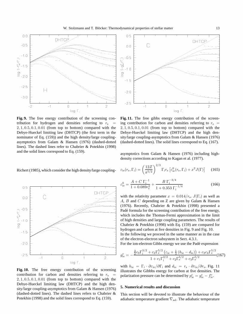
Fig. 9. The free energy contribution of the screening con-tribution for hydrogen and densities referring tors =2, 1, 0.5, 0.1, 0.01 (from top to bottom) compared with theDebye-Hueckel limiting law (DHTCP) (the first term in thenominator of Eq. (159)) and the high density/large coupling-asymptotics from Galam & Hansen (1976) (dashed-dottedlines). The dashed lines refer to Chabrier & Potekhin (1998)and the solid lines correspond to Eq. (159).

Richert (1985), which consider the high density/large coupling-

Fig. 10. The free energy contribution of the screeningcontribution for carbon and densities referring tors =2, 1, 0.5, 0.1, 0.01 (from top to bottom) compared with theDebye-Hueckel limiting law (DHTCP) and the high den-sity/large coupling-asymptotics from Galam & Hansen (1976)(dashed-dotted lines). The dashed lines refers to Chabrier&Potekhin (1998) and the solid lines correspond to Eq. (159).

Fig. 11. The free gibbs energy contribution of the screen-ing contribution for carbon and densities referring tors =2, 1, 0.5, 0.1, 0.01 (from top to bottom) compared with theDebye-Hueckel limiting law (DHTCP) and the high den-sity/large coupling-asymptotics from Galam & Hansen (1976)(dashed-dotted lines). The solid lines correspond to Eq. (167).

asymptotics from Galam & Hansen (1976) including high-density corrections according to Kagan et al. (1977).

εie(rs,Γi) =

(

12Z

π5/2

)2/3

Γirs[

ε0ie(rs,Γi) + x2J(Γ)]

(165)

ε0ie =A+ C Γ−1

i

1 + 0.089r2s+

B Γ−3/4i

1 + 0.353 Γ−1/4i

(166)

with the relativity parameterx = 0.014/rs. J(Γi) as well asA, B andC depending on Z are given by Galam & Hansen(1976). Recently, Chabrier & Potekhin (1998) presented aPade formula for the screening contribution of the free energy,which includes the Thomas-Fermi approximation in the limitof high densities and large coupling parameters. The results ofChabrier & Potekhin (1998) with Eq. (159) are compared forhydrogen and carbon at five densities in Fig. 9 and Fig. 10.In the following we proceed in the same manner as in the caseof the electron-electron subsystem in Sect. 4.3.1.For the ion-electron Gibbs energy we use the Pade expression

gcie = −32c0Γ

3/2i + c2Γ

5/2e

(

εie +13(hie − die)

)

+ c3c4Γ5/2e

1 + c1Γ3/2i + c2Γ

5/2e + c3Γ

5/2e

(167)

with hie = Γi · ∂εie/∂Γi and die = rs · ∂εie/∂rs. Fig. 11illustrates the Gibbbs energy for carbon at five densities. Thepolarization pressure can be determined bypcie = gcie − f c

ie.

5. Numerical results and discussion

This section will be devoted to illustrate the behaviour of theadiabatic temperature gradient∇ad. The adiabatic temperature


Fig. 12.Contributions of the isochoric specific heat in units ofkni for helium atT = 106K vs. density. The lines refer tothe ideal electrons (dashed dotted) and ions (long-dashed), theexchange and correlation (dashed), the ionic quantum correc-tion from Chabrier et al. (1992) (short-dashed), and the sumof those (solid). The curves with dots represent ionic quantumcorrections after Nagara et al. (1987).

gradient is a highly sensitive quantity, because it dependsonfirst and second-order derivations of the model Helmholtz freeenergy. Therefore it is well suited to test the quality of theex-plicit expressions derived in Sects. 3 and 4. The adiabatic gra-dient is a crucial ingredient for many applications. For instance,∇ad determines the Schwarzschild criterion for convective in-stability and an accurate evaluation is required for evolutionarycalculations of very-low mass stars. We restrict our compar-isons of the adiabatic temperature gradient to the EOS tablesgiven by Straniero (1988), Saumon et al. (1995), and Rogerset al. (1996). Further detailed comparisons can be found inSaumon et al. (1995) who compared their results for∇ad withthose of Fontaine et al. (1977), Dappen et al. (1988), and Magni& Mazzitelli (1979).

Fig. 12 shows the total isochoric specific heat according toEq. (20) as well as their various single contributions (in unitsof nik), i.e. electronic exchange and correlation terms (elec-tronic, ionic and screening part). We note that the discontinu-ity in the ionic correlation is caused by the fluid-solid phasetransition atΓ = 178 (Stringfellow et al. 1990), which canalso be observed for the adiabatic temperature gradient in thehigh-density region. The influence of quantum effects on thefluid-solid transition of the OCP is discussed in detail by Pol-lock & Hansen (1973), Lamb & Van Horn (1975), Nagara et al.(1987), Chabrier (1993) and Iyetomi et al. (1993). We chose forour numerical calculationsΓ = 178, which is based on an sim-ulated OCP without quantum effects (Stringfellow et al. 1990).The specific heat contribution according to the ionic correla-tion is monotonously increasing until the phase transitionof theOCP model. The first maximum atlog ρ ≈ 1.5 in the dashed

Fig. 13.High-density asymptotics of the adiabatic temperaturegradient∇ad vs. density for hydrogen, demonstrated along theisothermT = 5 · 103 K. The dashed line refers to the ideal andexchange terms only. The dashed-dotted (without ionic quan-tum effects), the solid (with ionic quantum corrections fromChabrier et al. 1992), and the short-dashed (with ionic quan-tum corrections from Nagara et al. 1987) lines take into accountcorrelations. For more explanation: see text.

Fig. 14.Adiabatic temperature gradient∇ad (without radiationand all terms in Eq. (20)) for hydrogen (solid line) atT =105.54K vs. density. The dashed line refers to Saumon et al.(1995) and the dashed-dotted line to Fontaine et al. (1977).

curve in Fig. 12 is determined essentially by the electronicex-change and electronic correlation. The influence of electronicexchange and correlation increases with decreasing tempera-tures. Quantum effects for the specific heat according to theions after Chabrier (1993) are illustrated by the dotted line inFig. 12, which can be seen also in Figs. 7 and 8. This contribu-tion is compensated at very high densities by the contributions


Fig. 15. Adiabatic temperature gradient∇ad (without radia-tion andall terms in Eq. (20)) for helium atT = 105.54Kvs. density. For the ionic quantum corrections the results fromChabrier et al. (1992) and from Nagara et al. (1987) (solid line)are used. The dotted line refers to Saumon et al. (1995) andthe dashed-dotted line to Fontaine et al. (1977). The ideality(long-dashed line) is shown for comparison.

Fig. 16. Adiabatic temperature gradient∇ad (with radiationandall terms in Eq. (20)) for helium atT = 106K vs. density.For the ionic quantum corrections the results from Chabrieretal. (1992) (solid line) and from Nagara et al. (1987) (short-dashed line) are used. The dotted line refers to Saumon et al.(1995), the triangles to Straniero (1988), the dashed-dotted lineto Fontaine et al. (1977), and the dots to Rogers et al. (1996).

of the ideal and the correlated ions. Considering ionic quantumcorrections calculated by Nagara et al. (1987) the isochoric spe-cific heat will be more strongly reduced as shown in Fig. 12.

We point out that the same behaviour appears for the adia-batic temperature gradient as indicated in Figs. 13 and 15-18.

Fig. 17. Adiabatic temperature gradient∇ad (with radiationand all terms in Eq. (20)) for carbon (solid line and short-dashed lines) atT = 106K vs. density. For the ionic quantumcorrections the results from Chabrier et al. (1992) (solid line)and from Nagara et al. (1987) (short-dashed line) are used. Thetriangles refers to Straniero (1988), the dashed-dotted line toFontaine et al. (1977), and the crosses to Lamb (1974).

Fig. 18. Adiabatic temperature gradient∇ad (with radiationand all terms in Eq. (20)) for carbon (solid line and short-dashed lines) atT = 107K vs. density. For the ionic quantumcorrections the results from Chabrier et al. (1992) (solid line)and from Nagara et al. (1987) (short-dashed line) are used. Thetriangles refers to Straniero (1988), the dashed-dotted line toFontaine et al. (1977), and the crosses to Lamb (1974).

Note, that although the ionic quantum correction calculated byChabrier et al. (1992) and Chabrier (1993) are valid only forthe solid phase we considered here also the fluid range in orderto illustrate the differences to the result of Nagara et al. (1987).Figs. 13-20 display isotherms of the adiabatic temperaturegra-


Fig. 19. Adiabatic temperature gradient∇ad (with radiationand all terms in Eq. (20)) for helium along the isothermsT = 106 (solid), 107 (dashed), and108K (dashed-dotted) vs.density.

Fig. 20. Adiabatic temperature gradient∇ad (with radiationandall terms in Eq. (20)) for a mixture of C/O=50/50 (massfractions) along the isothermsT = 107 (solid),107.5 (dashed),and108K (dashed-dotted) vs. density.

dient evaluated on the basis our analytic expressions giveninSect. 4 including the photonic contribution (Figs. 16-20) over abroad range of densities. As already mentioned, the representa-tions towards very high densities aimed at the purpose to showthe asymptotic behaviour of the potentials given by Eq. (20).The accurate description of plasmas at very high density re-gion requires the consideration of additional effects as electroncaptures and other processes (cf. Shapiro et al. 1983). Fig.13shows the high density asymptotics of the adiabatic tempera-ture gradient calculated by different approximations. Consid-ering ideal and exchange contributions we obtained the well

known value∇ad = 1/2, according to relativistic consider-ations. The limiting value∇ad = 3/8 is determined by in-clusion of the classical ionic correlation and∇ad = 1/4 isobtained with ionic quantum corrections given by Chabrier etal. (1992). In Fig. 14-18 we compare our formalism with datafrom other authors (Lamb 1974, Fontaine et al. 1977, Straniero1988, Saumon et al. 1995, Rogers et al. 1996) based on analyt-ical as well as numerical methods and valid for various densityand temperature ranges. The radiation contribution is dominantat high temperatures and low densities. The well-known limit-ing case of∇ad = 0.25 in the low-density limit depends on thetemperature in a strong manner.

The largest deviations for the adiabatic temperature gradi-ent are observed in the intermediate density region, that meansfor plasma parameter where e.g. correlation effects must bede-scribed by accurate expressions. It should be emphasized thatthe Pade technique is well suited to meet the challenging re-quirements of this - sometimes poorly known - density regime.

Fig. 19 shows the adiabatic temperature gradient for he-lium. In Fig. 20 we draw∇ad for a mixture of carbon and oxy-gen at high temperatures as appropriate for white dwarf interi-ors.

The temperatures and densities are chosen here accordingto the conditions for a fully ionized plasma. Nevertheless,ourEOS-formalism can be applied for the conditions of a partiallyionized plasma (lower temperatures) provided additional termsin Eq. (20) are considered and are solved in connection withthe formalism of the dissoziation- and ionization equilibrium(Beule et al. 1999).

6. Summary

Our aim was to provide data for the thermodynamical poten-tials summarized in Eq. (20) which are applicable to, e.g., stel-lar interiors (fully ionized regions). For the Helmholtz free en-ergy, the Gibbs free energy, and the pressure (equation of state),expressions for each term in Eq. (20), i.e. ideality, exchangeand correlation, have already been presented in paper I. In thispaper we have improved our Pade Approximants for the corre-lation contributions and continued to present formulae fortheexplicit calculation of the internal energy, reciprocal compress-ibility (bulk modulus), coefficient of strain, and the specificheat. Further results using our calculational concept for the adi-abatic temperature gradient for fully ionized plasmas are pre-sented by Stolzmann & Blocker (1998). The extension of ourformalism to the partially ionized region is in progress.

Acknowledgements. One of us (W.S.) acknowledges funding by theDeutsche Forschungsgemeinschaft (grant Scho 394/18).

References

Beule D., Ebeling W., Forster A., Juranek H., Nagel S., Redmer R.,Ropke G., 1999, Phys. Rev. B59, 14177

Blinnikov S.I., Dunina-Barkovskaya N.V., Nadyozhin D.K.,1996,ApJS 106, 171

Brami B., Hansen J.P., Joly F., 1979, Physica 95A, 505


Chabrier G., 1993, ApJ. 414, 695Chabrier G., Ashcroft N.W., DeWitt H.E., 1992, Nat. 360, 48Chabrier G., Potekhin A.Y., 1998, Phys. Rev. E58, 4941Chandrasekhar S., 1939,An Introduction to the Study of Stellar Struc-

ture, University of Chicago Press, ChicagoCohen E.G.D., Murphy T.J., 1969, Phys. Fluids 12, 1404Cox J.P., Giuli R.T., 1968,Principles of Stellar Structure, Vol.1 & 2,

Gordon and Breach, New YorkDappen W., Hummer D.G., Mihalas D., Weibel-Mihalas B., 1988,

ApJ. 332, 261DeWitt H.E., Slattery W.L., 1999, Contrib. Plasma Phys. 39,97Ebeling W., Kraeft W.D., Kremp, D., 1976,Theory of Bound States

and Ionization Equilibrium in Plasmas and Solids, Akademie Ver-lag, Berlin

Ebeling W., 1993, Contrib. Plasma Phys. 33, 492Ebeling W., Richert W., 1985, phys. stat. sol. (b), 128, 467Ebeling W., Stolzmann W., Forster A., Kasch M., 1999, Contrib.

Plasma Phys. 39, 287Eggleton P.P., Faulkner J., Flannery B.P., 1973, A&A 23, 325Eliezer S., Ghatak A., Hora H., 1986,An Introduction to Equation

of State: Theory and Applications, Cambridge University Press,Cambridge

Fontaine G., Graboske H.C., Van Horn H.M., 1977, ApJS 35, 293Galam S., Hansen J.P., 1976, Phys. Rev. A14, 816Graboske H.C. Jr., Olness R.J., Grossman A.S., 1975, ApJ. 199, 255Hansen J.P., 1972, Phys. Lett. 41A, 18, 213Hansen J.P., 1973, Phys. Rev. A8, 3096Hansen J.P., Vieillefosse P., 1975, Phys. Lett. 53A, 187Iben I., Tutukov V.A.,1984, ApJ. 282, 615Ichimaru S., 1993, Rev. Mod. Phys. 65, 255Ichimaru S., 1994,Statistical Plasma Physics, Vol. II: Condensed

Plasmas, Addison-Wesley Publishing Company, Reading, Mas-sachusetts

Iyetomi H., Ogata S., Ichimaru S., 1993, Phys. Rev. B47, 11703Johns S.M., Ellis P.J., Lattimer J.M., 1996, ApJ 473, 1020Kagan Yu.M., Pushkarev V.V., Kholas A., 1977, Zh. Eksper. Teor. Fiz.

73, 967Kahlbaum T., 1996, inPhysics of Strongly Coupled Plasmas, eds.

W.D. Kraeft and M. Schlanges, World Scientific, Singapore, p.99

Kalitkin N.N., Ritus I.V., 1986, Zh. vychislit. Mat. i. mat.Fiz. 3, 461Kirkwood J.G., 1933, Phys. Rev. 44, 31Kovetz A., Lamb D.Q., Van Horn H.M., 1972, ApJ 174, 109Lamb D.Q., 1974, Ph.D. thesis, University of RochesterLamb D.Q., Van Horn H.M., 1975, ApJ 200, 306Magni G., Mazzitelli T., 1979, Astron. Astrophys. 72, 134Miralles J.A., Van Riper K.A., 1996, ApJS 105, 407Nagara H., Nagata Y., Nakamura T., 1987, Phys. Rev. A36, 1859Perrot F., Dharma-wardana M.W.C., 1984, Phys. Rev. A30, 2619Pollock E.L., Hansen J.P., 1973, Phys. Rev. A8, 3110Rogers F.J., Swenson F.J., Iglesias C.A., 1996, ApJ 456, 902Salpeter E.E., Zapolsky H.S., 1967, Phys. Rev. 158, 876Saumon D., Chabrier G., Van Horn H.M., 1995, ApJS 99, 713Shapiro S.L., Teukolsky S.A., 1983,Black Holes, White Dwarfs, and

Neutron Stars, Wiley, New YorkSlattery W.L., Doolen G.D., DeWitt H.E., 1980, Phys. Rev. A21, 2087Stolzmann W., Blocker T., 1994, inThe Equation of State in Astro-

physics, eds. G. Chabrier and E. Schatzman, Cambridge Univer-sity Press, Cambridge, p. 606

Stolzmann W., Blocker T., 1996a, A&A 314, 1024 (paper I)

Stolzmann W., Blocker T., 1996b, inPhysics of Strongly CoupledPlasmas, eds. W.D. Kraeft and M. Schlanges, World Scientific,Singapore, p. 95

Stolzmann W., Blocker T., 1998, inStrongly Coupled Coulomb Sys-tems, eds. G.J. Kalman, J.M. Rommel, and K. Blagoev, PlenumPress, New York, p. 265

Stolzmann W., Rosler M., 1998, inStrongly Coupled Coulomb Sys-tems, eds. G.J. Kalman, J.M. Rommel, and K. Blagoev, PlenumPress, New York, p. 673

Stolzmann W., Ebeling W., 1998, Phys. Lett. A 248, 242Stolzmann W., Blocker T., 1999, Contrib. Plasma Phys. 39, 105Straniero O., 1988, A&A 76, 157Stringfellow G.S., DeWitt H.E., Slattery W.L., 1990, Phys.Rev. A41,

1105.Vosko S.H., Wilk L., Nusair M., 1980, Can. J. Phys. 58, 1200Yakovlev D.G., Shalybkov D.A., 1989, Sov. Sci. Rev. E. Astrophys.

Space Phys. 7, Harwood Academic Publishers, LondonWigner E.P., 1932, Phys. Rev. 40, 749

astronomy and 12 (02.05.2; 02.16.1; 08.09.3; 08.05 ... - … · technique of pade´ approximants as...

Documents