backward bifurcation in sir endemic models : this thesis ... · stages of this thesis. i also would...
TRANSCRIPT

Copyright is owned by the Author of the thesis. Permission is given for a copy to be downloaded by an individual for the purpose of research and private study only. The thesis may not be reproduced elsewhere without the permission of the Author.
BACKWARD BIFURCATION IN SIR ENDEMIC MODELS
THIS THESIS IS PRESENTED IN PARTIAL FULFILLMENT OF THE REQUIREMENTS FOR THE
DEGREE OF
MASTERS OF INFORMATION SCIENCE
IN
MATHEMATICS
AT MASSEY UNIVERSITY, ALBANY, AUCKLAND,
NEW ZEALAND.
SAMEEHA QAISER SIDDIQUI
2008
@Copyright By Sameeha Qaiser Siddqiui

Abstract
In the well known SIR endemic model, the infection-free steady state is globally stable
for R0 < 1 and unstable for R0 > 1 . Hence, we have a forward bifurcation when R0 = 1 .
When R0 > 1 , an asymptotically stable endemic steady state exists. The basic repro
duction number R0 is the main threshold bifurcation parameter used to determine the
stability of steady states of SIR endemic models.
In this thesis we study extensions of the SIR endemic model for which a backward
bifurcation may occur at R0 = 1 . We investigate the biologically reasonable conditions
for the change of stability. We also analyse the impact of different factors that lead to a
backward bifurcation both numerically and analytically. A backward bifurcation leads to
sub-critical endemic steady states and hysteresis.
We also provide a general classification of such models, using a small amplitude ex
pansion near the bifurcation. Additionally, we present a procedure for projecting three
dimensional models onto two dimensional models by applying some linear algebraic tech
niques. The four extensions examined are: the SIR model with a susceptible recovered
class; nonlinear transmission; exogenous infection; and with a carrier class.
Numerous writers have mentioned that a nonlinear transmission function in relation
to the infective class, can only lead to a system with an unstable endemic steady state. In
spite of this we show that in a nonlinear transmission model, we have a function depending
on the infectives and satisfying certain biological conditions, and leading to a sub-critical
endemic equilibriums.

Acknowledgments
I would like to thank my supervisor Professor Mick Roberts for his patience, for always
being there and providing many relevant suggestions and worthy opinions throughout all
stages of this thesis.
I also would like to thank to the department of I IMS at the Massey University (Al
bany) for giving me the opportunity to pursue my postgraduate studies and wish to thank
Haydn Cooper for his valuable comments.
I am also grateful to my family, my husband Arsh and my baby Talish, for without
their help and support this study would have been impossible.

CONTENTS
Contents 1
2
3
Introduction
1 . 1
1 .2
1 . 3
The Basic SIR Model .
The SIR Epidemic Model .
The SIR Endemic Model .
1 . 3 . 1
1 . 3 .2
1 .3 .3
1 .3 .4
1 .3 .5
Steady State Solutions
Stability . . . . . . . .
Bifurcation Analysis
Phase-Plane Analysis .
Summary • • • • 0 • 0
2D Extensions
2 . 1
2 .2
2 .3
2 .4
The SIR model with Susceptible R Class
2 . 1 . 1 Steady State Solutions
2 . 1 . 2 Saddle Node Equation
2 . 1 .3 Stability . . . . . . . .
2 . 1 .4 Bifurcation Analysis
2 . 1 . 5 Phase-Plane Analysis .
The SIR model with Nonlinear Transmission Class . 2 .2 . 1 Steady State Solutions
2 .2 .2 Saddle Node Equation
2 .2 .3 Stability . . . . . . . .
2 .2 .4 Bifurcation Analysis
2 .2 .5 Phase-Plane Analysis .
The SIR model with Exogenous Infection Class
2 .3 . 1 Steady State Solutions
2 .3 .2 Saddle Node Equation
2 .3 .3 Stability . . . . . . . .
2 .3 .4 Bifurcation Analysis
2 .3 .5 Phase-Plane Analysis .
Summary • • • • • • • 0 • • •
General Analysis of 2D Models
3 . 1 Susceptible R Class . . . . . .
3 .2 N onlinear Transmission Class
3 .3 Exogenous Infection Class . .
iii
CONTENTS
1
1
2
5
6
7
7
8
8
10
1 0
1 1
1 1
1 2
14
15
18
19
20
2 1
22
22
26
27
28
29
3 1
3 1
34
36
36
39
42

CONTENTS
4
5
6
3D Extensions
4 . 1
4 . 2
4 .3
4 .4
4 .5
SEIR model • • 0 • • • • • • •
4. 1 . 1 Steady State Solutions
4. 1 . 2 Saddle Node Equation
4 . 1 .3 Stability . . . . . . . .
4 . 1 .4 Bifurcation Analysis
4 . 1 . 5 Phase-Plane Analysis .
The SEIR model with Partial Recovery .
4 .2 . 1 Steady State Solutions
4 .2 .2 Saddle Node Equation
4 .2 .3 Stability . . . . . . . .
4 .2 .4 Bifurcation Analysis
4 .2 .5 Phase-Plane Analysis .
SEIR model with Full Recovery
4 .3 . 1 Steady State Solutions
4 .3 .2 Saddle Node Equation
4 .3 .3 Stability . . . . . . . .
4 .3 .4 Bifurcation Analysis
4 .3 .5 Phase-Plane Analysis .
The SIR Model with Carrier Class .
4 .4 . 1 Steady State Solutions
4.4 .2 Saddle Node Equation
4.4 .3 Stability . . .
4 .4 .4 Examples 1 , 2
Summary • • • • 0 •
General Analysis of 3D Models
5 . 1 The SEIR model . . . . . . . .
5 . 2 SEIR model with Partial Recovery
5 .3 SEIR model with Full Recovery . .
5 .4 The SIR Model with Carrier Class .
Discussion
lV
CONTENTS
45
45 46
46
47
49
50
54
54
55
56
58
59
62
62
63
64
65
69
69
70
70
71
72
87
88 88
90
94
97
101

LIST OF TABLES
List of Tables 1
2
3
4
5
6
7
8
9
Summary of the notations used in the SIR Model
Parameter values for susceptible R class. . . . . .
Parameter values for nonlinear transmission class.
Parameter values for exogenous infection class.
Frequently Used Notation in Chapters 3 and 5 . .
Parameter values for the SEIR model. • • 0 • • •
Parameter values for the SEIR model with partial recovery.
Parameter values for the SEIR model with full recovery . .
Parameter values for the SIR model with carrier class.
V
LIST OF TABLES
2
12
21
28
37
47
55
63
72

LIST OF FIGURES LIST OF FIGURES
List of Figures 1
2
3
Phase-Plane for SIR epidemic model when R0 = 5 .
Triangle Invariance of SIR endemic model. . . . . .
Bifurcation analysis for SIR endemic model. Stable infection-free steady
state for R0 < 1 ; unstable infection-free i and stable endemic steady state
4
6
i* for R0 > 1 . . . . . . . . . . . . . . . . . . . . . . . . . . . . . . . . . . . 8
4 Phase-Plane for SIR endemic model when: (a) R0 = 0 .5 < 1 ; (b) R0 =
2 > 1 . Other parameter values are p, = 0 .02 and 1 = 0.05 . . . . . . . . . . . 9
5 Bifurcation diagram for the SIR model with susceptible R class giving
curves (R0 , s*) and (R0 , i*) . Broken lines signify unstable steady state
while unbroken & dotted lines are stable ones. Light dark arrow points
downward at R0 = Rsaddle where two endemic equilibriums coincide. The
(R0 , s*) and (R0, i*) curves have backward bifurcations when P > Pcrit
6
7
8
9
10
11
12
13
14
where Pcrit = 1 + � · . . . . . . . . . . . . . . . . . . . . . . . . . . . . . . 14
Phase-Plane for the SIR model with susceptible R Class for P = 0 < Pcrit when: (a) R0 = 0 .8 < 1 ; (b) R0 = 1 . 2 > 1. . . . . . . . . . . . . . . . . . . 15
� Phase-Planes for susceptible R class for P = 2 when: (a) R0 = 0 .8 < 1 ;
(b) Ro = 1 . 2 > 1 . . . . . . . . . . . . . . . . . . . . . . . . . . . . . . . . . 16
Phase-Planes for susceptible R class for P = Pcrit when: (a) Ro = 0 .8 < 1 ;
(b) R0 = 2 > 1 . . . . . . . . . . . . . . . . . . . . . . . . . . . . . . . . . . 16
Phase-Planes for susceptible R class for P = 2 .8 > Pcrit when: (a) R0 =
0 .5 < Rsaddle ; (b) Ro = Rsaddle · · · · · · · · · · · · · · 17
Phase-Planes for susceptible R class for P = 2 .8 > Pcrit when: (a) Rsaddle < Ro = 0 .92 < 1 ; (b) R0 = 2. . . . . . . . . . . . . . . . . . . . . 17 Bifurcation diagram for the SIR model with nonlinear transmission class.
Labels are as in Fig. 5 . For this class, Pcrit = 1 + �· . . . . . . . . . . . . 23
Phase-Planes for the SIR model with nonlinear transmission class for P =
0 < Pcrit when: (a) R0 = 0 .8 < 1 ; (b) R0 = 1 . 2 > 1 . . . . . . . . . . 24 � Phase-Planes for nonlinear transmission class for P = 2 when: (a)
Ro = 0 .8 < 1 ; (b) R0 = 1 .2 > 1 . . . . . . . . . . . . . . . . . . . . . . . . 24
Phase-Planes for nonlinear transmission class for P = 3 .5 = Pcrit when:
(a) Ro = 0 .8 < 1 ; (b) R0 = 1 . 2 > 1 . . . . . . . . . . . . . . . . . . . . . . 25
15 Phase-Plane for nonlinear transmission class for P > Pcrit when: (a) R0 =
0 .5 ; (b) Ro = Rsaddle = 0 .951919 . . . . . . . . . . . . . . . . . . . . 25
16 Phase-Plane for nonlinear transmission class for P > Pcrit when: (a) Rsaddle < Ro = 0 .96 < 1 ; (b) Ro = 1 . 2 > 1 . . . . . . . . . . . . . . 26
vi

LIST OF FIGURES LIST OF FIGURES
17 Bifurcation diagram for the SIR model with exogenous infection class. La-bels are as in Fig. 5. The critical value of P for this class is v(:tf.L) . . . . . 30
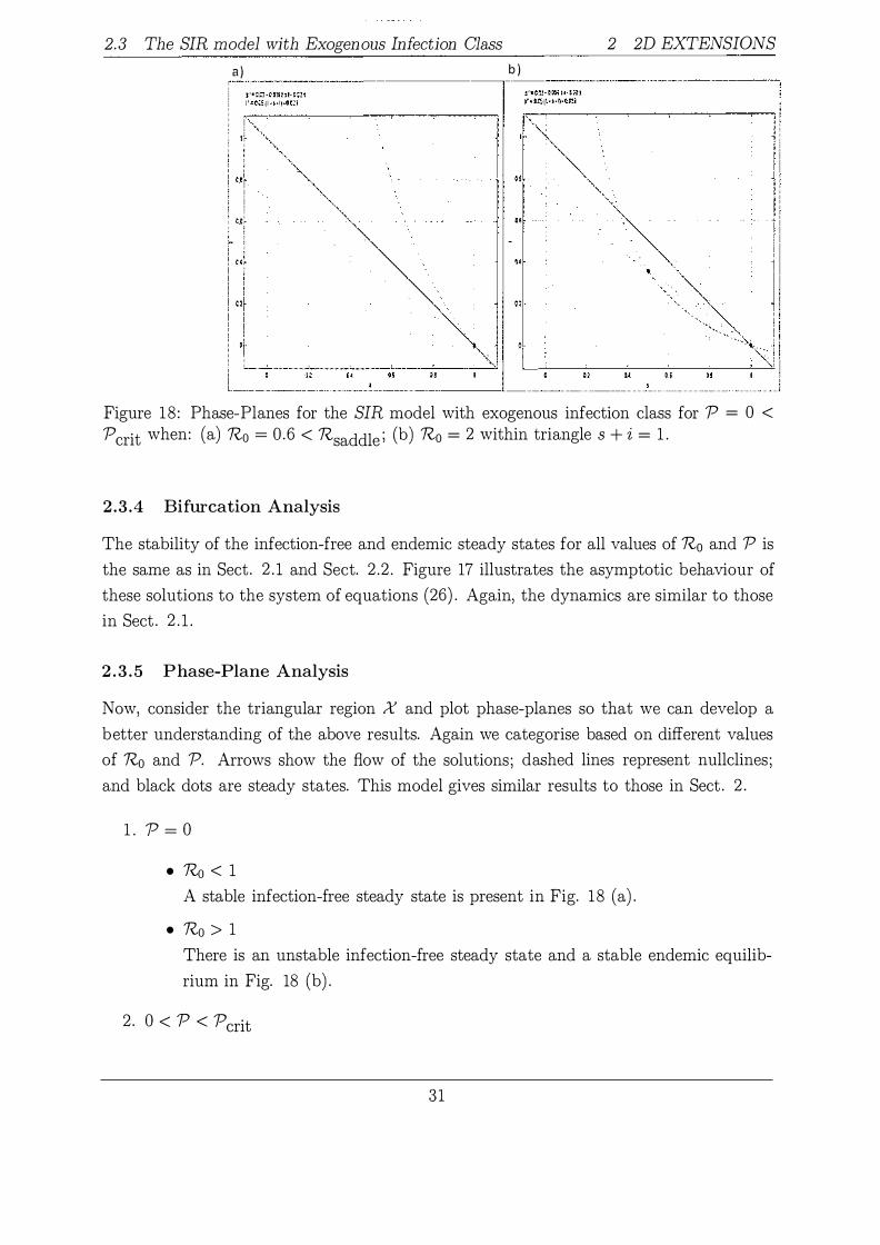
18 Phase-Planes for the SIR model with exogenous infection class for P = 0 < Pcrit when: (a) Ro = 0 .6 < Rsaddle ; (b) R0 = 2 within triangles + i = 1 . 31
19 Phase-Planes for exogenous infection class for P = 5 < Pcrit when: (a) Ro = 0 .6 < Rsaddle ; (b) R0 = 1 .2 . . . . . . . . . . . . . . . . . . . . 32
20 Phase-Planes for exogenous infection class for P = Pcrit = 8 .75 when: (a)
Ro = 0.6 < Rsaddle ; (b) Ro = 2. . . . . . . . . . . . . . . . . . . . . 32
21 Phase-Planes for exogenous infection class for P = 14 > Pcrit when: (a)
Ro = 0.6 < Rsaddle ; (b) Ro = 0.9838 = Rsaddle · . . . . . . . . . . 33
22 Phase-Planes for exogenous infection class for P = 14 > Pcrit when: (a)
Rsaddle < Ro = 0.99 < 1 ; (b) Ro = 1 . 2 > 1 is of interest . . . . . . . . 33
23 Enlarged top-center part of Figure 5. A clearer view for s t < 0 , and the
values for R01 as we perturb the variable i*. Unbroken lines show stable
steady states while broken lines signify unstable. The curve R01 < 0 when
P > Pcrit and curve R01 > 0 when P < Pcrit · . . . . . . . . . . . . . . . 39
24 Enlarged diagram taken from Fig. 1 1 . Labels are as in Fig. 23. . . . . . . 41
25 An enlarged top-center portion of the bifurcation fig. (17) . Labels are as
in Fig. 23. . . . . . . . . . . . . . . . . . . . . . . . . . . . . . . . . . . . . 44
26 Bifurcation Diagram for the SEIR model. Curves are s* and i* as the
functions of R0 . Continuous lines show stable steady state and broken
lines are unstable steady states. There are curves for P < Pcrit ' P = Pcrit and P > Pcrit · For this model, Pcrit = v(:tv) . . . . . . . . . . . . . . . . . 50
27 Phase-Planes for the SEIR Model for P = 0: when (a) R0 = 0 .6 < 1 ; (b)
Ro = 1 . 2 > 1. . . . . . . . . . . . . . . . . . . . . . . . . . . . . . . . . . . 5 1
28 Phase-Planes for the SEIR Model for P = 5 < Pcrit when: (a) R0 = 0 .6 <
1 ; (b) R0 = 1 . 2 > 1 . . . . . . . . . . . . . . . . . . . . . . . . . . . . . . . . 5 1
29 Phase-Planes for the SEIR Model for P = 8 .75 = Pcrit when: (a) R0 = 0 .6 < 1 ; (b) R0 = 1 . 2 > 1 . . . . . . . . . . . . . . . . . . . . . . . . . . . . 52
30 Phase-Planes for the SEIR Model for P > Pcrit when: (a) R0 = 0.8 < Rsaddle ; (b) Rsaddle = 0.977 < 1 . · · · · · · · · · · · · · · · · · · · · · · 52
31 Phase-Planes for the SEIR Model for P > Pcrit when: (a) R0 = 0 .987 < 1 ; (b) R0 = 1 . 2 > 1 . . . . . . . . . . . . . . . . . . . . . . . . . . . . . . . . 53
32 Bifurcation Diagram for the SEIR model with partial recovery. Labels are
as in Figure 26. This model have P crit = [(f.L+'Y��i�l)"v'Y] . . . . . . . . 58
33 Phase-Plane for the SEIR Model with partial recovery for P = 0 when: (a)
Ro = 0.7 < 1; (b) R0 = 1 .2 > 1. . . . . . . . . . . . . . . . . . . . . 59
Vll

LIST OF FIGURES LIST OF FIGURES
34
35
36
37
38
39
40
41
42
43
44
45
46
47
48
49
� Phase-Plane for the SEIR Model with partial recovery for P = 1 .3 = f1 when: (a) R0 = 0 .7 < 1 ; (b) R0 = 1 .2 > 1 . . . . . . . . . . . . . . . . . . . 60
Phase-Plane for the SEIR Model with partial recovery for P = 2 .6 = Pcrit when: (a) R0 = 0 .7 < 1 ; (b) R0 = 1 .2 > 1 . . . . . . . . . . . . . . . . . . 60
Phase-Plane for the SEIR Model with partial recovery for P > Pcrit when:
(a) Ro = 0 .7 < Rsaddle ; (b) Rsaddle = 0 .9545 < 1 . . . . . . . . . . . . . 6 1
Phase-Plane for the SEIR Model with partial recovery for P > Pcrit when: (a) Rsaddle < Ro = 0 .98 < 1 ; (b) Ro = 1 .2 > 1 . . . . . . . . . . . . . . . 6 1 Bifurcation Diagram for the SEIR model with full recovery. The critical
value of P crit = (J.L+I'��+v) . . . . . . . . . . . . . . . . . . . . . . . . . 66
Phase-Planes for the SEIR Model with full recovery for P = 0 when: (a)
R0 = 0.7 < 1 ; (b) R0 > 1 . . . . . . . . . . . . . . . . . . . . . . . . . . . . 66 � Phase-Planes for the SEIR Model with full recovery for P = 0 .98 = f1
when: (a) R0 = 0 .7 < 1 ; (b) R0 = 2 > 1 . . . . . . . . . . . . . . . 67
Phase-Plane for the SEIR Model with full recovery for P = 1 . 96 = Pcrit when: (a) R0 = 0 .7 < 1 ; (b) R0 = 2 > 1 . . . . . . . . . . . . . . . . . . . 67
Phase-Plane for the SEIR Model with full recovery for P > Pcrit when:
(a) Ro = 0. 7 < Rsaddle ; (b) Rsaddle = 0 .9308 < 1 . . . . . . . . . . . . . 68
Phase-Plane for the SEIR Model with full recovery for P > Pcrit when: (a) Rsaddle < Ro = 0 .98 < 1 ; (b) Ro = 2 > 1 . . . . . . . . . . . . . . . . 68 Bifurcation diagram for the SIR model with carrier class (Example 1 ) for
the function q(x*) = 1 - e-o.gx*. We show 1 - s* as a function of R0 .
Backward bifurcation occurs when P > Pcrit = /'���) at (R0 , 1 - s*) = ( 1 ,
0 ) . 0 0 0 0 0 0 0 0 0 0 0 0 0 0 0 0 0 0 0 0 0 0 0 0 0 0 0 0 0 0 0 0 0 0 0 0 0 0 0 0 75
Phase-Plane for the Example 1 for P = 0 < Pcrit when: (a) Ro = 0.7 ; (b)
R0 = 1 . 1 . . . . . . . . . . . . . . . . . . . . . . . . . . . . . . . . . . . . . 76
Phase-Plane for the Example 1 for P = 0 .8333 = Pcrit when: (a) R0 = 0 .7 ;
(b) R0 = 1 . 1 . . . . . . . . . . . . . . . . . . . . . . . . . . . . . . . . . . . 77
Phase-Plane for the Example 1 for P = 1 . 6 > Pcrit when: (a) Ro = 0 .7 <
1 ; (b) Ro = Rsaddle = 0 .8299 < 1 . . . . . . . . . . . . . . . . . . . . . . . 77
Phase-Plane for the Example l for P = 1 .6 > Pcrit when: (a) Rsaddle <
Ro = 0.95 < 1 ; (b) R0 = 1 . 1 > 1 . . . . . . . . . . . . . . . . . . . . . . . . 78
Time-series plots for the carrier class Example 1 . For P = 0 < P crit :
(a) Ro = 0 .7 < 1 ; (b) Ro = 1 . 1 > 1 and For P = 0 .8333 = Pcrit : (c)
Ro = 0 .7 < 1 ; (d) R0 = 1 . 1 > 1 . . . . . . . . . . . . . . . . . . . . . . . . . 78
viii

LIST OF FIGURES LIST OF FIGURES
50 Time-series for q(x) = 1 - e-0·9x the carrier class Example 1. For P = 1 . 6 > Pcrif (a) Ro = 0 .6 < 1 ; (b) Rsaddle = R0 = 0 .8299 < 1 ; (c) Rsaddle < Ro = 0 .95 < 1; (d) Ro = 1 . 1 > 1 . . . . . . . . . . . . . . . . . . 79
51 Bifurcation Diagram for the carrier class for the function q(x*) = x;;:2 . In this diagram, 1 - s* is plotted against R0 . Backward bifurcation occurs
when P > Pcrit = 0 .9 for q'(O) = 0 . Multiple endemic steady states exist
in the region of Rsaddle < R0 < 1 . 19 . . . . . . . . . . . . . . . . . . . . . . 82
52 Phase-Planes for the Example 2 for P = 0 < Pcrit when: (a) R0 = 0 .7 <
1 . 19 ; (b) R0 = 1 . 2 > 1 . 19 . . . . . . . . . . . . . . . . . . . . . . . . . . . . 83
53 Phase-Planes for the Example 2 for P = 0 .9 = Pcrit when: (a) Ro = 0 .7 <
1 . 19 ; (b) R0 = 1 . 2 > 1 . 19 . . . . . . . . . . . . . . . . . . . . . . . . . . . . 84
54 Phase-Planes for the Example 2 for P = 1.8 > Pcrit when: (a) R0 = 0 .7 <
1 . 19 ; (b) Rsaddle = Ro = 1 .09 < 1 . 19 . . . . . . . . . . . . . . . . . . . . . 84 55 Phase-Planes for the Example 2 for P = 1 . 8 > Pcrit when: (a)Rsaddle <
R0 = 1 . 17 < 1 . 19 ; (b) R0 = 1 . 2 > 1 . 19 . . . . . . . . . . . . . . . . . . . . . 85
56 Time-series plots for the carrier class Example 2. For P = 0 < Pcrif (a) R0 = 0 .7 < 1 ; (b) Ro = 1 . 2 > 1 and For P = 0 .9 = Pcrit : (c)
Ro = 0. 7 < 1; (d) R0 = 1. 2 > 1. . . . . . . . . . . . . . . . . . . . . . . . . 86
57 Time-series plots for the carrier class Example 2 for P = 1 . 8 > Pcrit : (a)
R0 = 0.7 < 1; (b) R0 = Rsaddle = 1 .09 < 1 . 19 ; (c)Rsaddle < Ro = 1 . 16 < 1 . 19 ; (d) R0 = 1 . 2 > 1 . . . . . . . . . . . . . . . . . . . . . . . . . 86
58 An enlarged top-center portion of Fig. 26. In this sketch , it is clearly shown
that st < 0 , and R01 < 0 give backward bifurcation, while R01 > 0 give
forward bifurcation. . . . . . . . . . . . . . . . . . . . . . . . . . . . . . . 9 1
59 Enlarged top-center portion of Bifurcation diagram 32. The critical value
Pcrit = (M+ ���l+:l)- K,[V . . . . . . . . . . . . . . . . . . . . 94
60 Blow up of the bifurcation diagram 38. Labels are as in Fig. 26. The
·t · l 1 f P f th· 1 · P (M+ r) (�Jo+ v) 97 en Ica va ue o or IS c ass IS crit = V[ . . . . . .
61 A top-center blow up of Bifurcation diagram 44. Labels are as in Fig. 26.
The critical va}ue for P is Pcrit = r�'(x�)' . . . . . . . . . . . . 100
IX

1 lntrod uction
1.1 The Basic SIR Model
1 INTRODUCTION
There are many infections for which the recovered individuals attain an immunity against
the infection. This type of infection can be modeled by the SIR model, which is based
on the classic epidemic theory of Kermack and McKendrick [7] . This model has played
an important role in mathematical epidemiology. In this model, a closed population of
constant size is subdivided into three classes: susceptible ( S) individuals that may suffer
infection; infected (I) individuals that transmit infection to the susceptibles; and removed
( R) individuals who are recovered and immune or dead.
The proportions in each class at time t are denoted as s(t) , i(t) and r(t) respectively.
The differential equations representing this system are
ds f-l - j3si - f-LS, ( 1 ) -
dt di
j3si - (r + f-l ) i, -
dt dr
[i- f-tr. -
dt
As r ( t) = 1 - s ( t) - i ( t) , the system is two dimensional. The parameters are birth and
death rate (M > 0) , recovery rate (r > 0) and contact rate (/3 > 0) (See Table 1 ) . The
basic reproduction number R0 = +/3 , is defined to be the expected number of secondary p, I cases generated from an infective case in a susceptible population [12] .
Now, if f-l << [, then this system becomes the SIR epidemic model, which describes
the sudden rise and fall of an infection in a closed population, for example influenza,
plague etc [3] . If, on the other hand, f-l � [, then we have the SIR endemic model, where
an infection tends to persist in a population for a longer period, for example leprosy or
tuberculosis. Endemic models focus on when there is no net change in the number of
individuals in the infective class, so prevalence of infection remains constant [1 1] .
Thesis Outline
In this thesis, we review properties of the SIR epidemic model in Sect. 1 . 2 briefly, and the
endemic model in Sect . 1 . 3 in detail as this model is the primary subject of this thesis.
In Chapters 2 and 4 we present the two and three dimensional extensions of the SIR
1
1 .2 The SIR Epidemic Model
Variables Description s Number of susceptibles I Number of infectives R Number of recovered people with immunity
Parameters Description
fL Birth and death rate I Recovery rate (3 Transmission or contact rate
Ro Basic reproduction number
1 INTRODUCTION
Proportions s(t) i(t) r(t)
Dimensions time 1
time-1
time-1
-
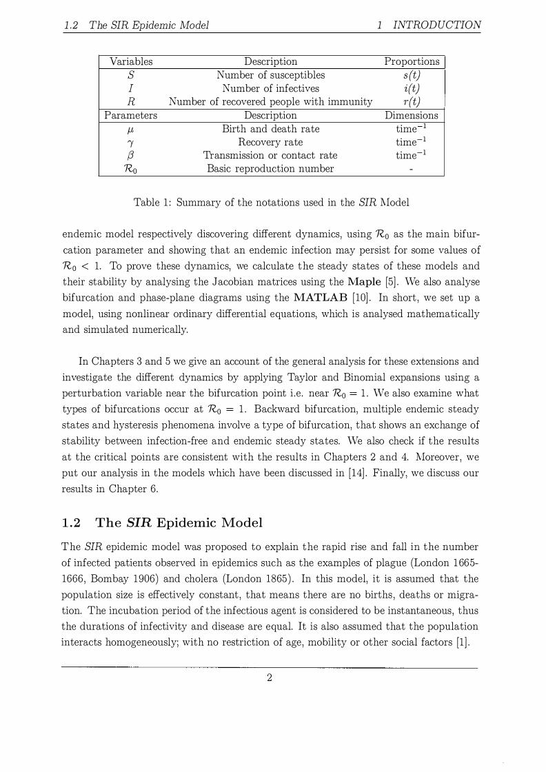
Table 1 : Summary of the notations used in the SIR Model
endemic model respectively discovering different dynamics, using R0 as the main bifur
cation parameter and showing that an endemic infection may persist for some values of
R0 < 1. To prove these dynamics, we calculate the steady states of these models and
their stability by analysing the J acobian matrices using the Maple [5] . We also analyse
bifurcation and phase-plane diagrams using the MATLAB [10] . In short , we set up a
model, using nonlinear ordinary differential equations, which is analysed mathematically
and simulated numerically.
In Chapters 3 and 5 we give an account of the general analysis for these extensions and
investigate the different dynamics by applying Taylor and Binomial expansions using a
perturbation variable near the bifurcation point i .e . near R0 = 1 . We also examine what
types of bifurcations occur at R0 = 1 . Backward bifurcation, multiple endemic steady
states and hysteresis phenomena involve a type of bifurcation, that shows an exchange of
stability between infection-free and endemic steady states. We also check if the results
at the critical points are consistent with the results in Chapters 2 and 4. Moreover, we
put our analysis in the models which have been discussed in [14] . Finally, we discuss our
results in Chapter 6 .
1.2 The SIR Epidemic Model
The SIR epidemic model was proposed to explain the rapid rise and fall in the number
of infected patients observed in epidemics such as the examples of plague (London 1665-
1666 , Bombay 1906) and cholera (London 1865) . In this model, it is assumed that the
population size is effectively constant , that means there are no births , deaths or migra
tion. The incubation period of the infectious agent is considered to be instantaneous, thus
the durations of infectivity and disease are equal. It is also assumed that the population
interacts homogeneously; with no restriction of age, mobility or other social factors [1] .
2

1 . 2 The SIR Epidemic Model 1 INTRODUCTION
Starting with the system (1 ) of the SIR epidemic model; we assume that fJ = 0 , then
we have
ds -j3si, (2) -
dt di
j3si- 1i, (3) -dt dr - IZ . dt
As we assume that the population is of constant size we have r(t) = 1 - s(t) - i(t) . The
rate parameters for the transition between the three classes are j3 and 1 (see Sect . 1 . 1 ) .
The term -j3si describes a transmission of infection due to the interaction between sus
ceptibles and infectives . The term - 1i describes the recovery from an infection [3] .
Observe that if � � 0 at t = 0, then there is no epidemic, while if � > 0 at t = 0 , then
an epidemic occurs i .e . an increase in infective individuals. Also, equation (2) implies
that if the term -j3si = 0, then we get either s = 0 or i = 0. If i = 0 , then � = 0, which
means an infection-free population will remain infection-free forever, on the contrary if
i =I= 0 and s > �' then � > 0 , which is a threshold condition [11 ] . Therefore an epidemic
occurs for s0 > � where s0 is the initial number of susceptibles. Thus, the expected
number of infections produced by one infected individual is R0 = fl. and s(O) = s0 [ ll] . I
The basic reproduction number R0 determines whether an epidemic is expected to
occur in the population or not , thus an epidemic arises when R0s0 > 1 as shown in [2] .
Moreover, equations (2) & (3) show that
d(s + i) dt
= -IZ ,
demonstrating that s + i is decreasing when i > 0 (see Fig. 1 ) . We derive an expression
for the final size of an epidemic. Firstly, we combine equations (2) & (3) to get
di ds
=? di
j3si - 1i 1 -�--'-- = -1 + --j3si j3s (-1 + 2) ds = (-1 + -
1 ) ds. j3s Ros
Integrating, using the initial conditions, and then taking limits gives,
. 1 z = -s +
Ro logs + K,
3

1 . 2 The SIR Epidemic Model 1 INTRODUCTION
s'•M0.25tl I'"' 0.23 si· 0.05 i
Figure 1: Phase-Plane for SIR epidemic model when 1?0 = 5.
1 1 K = io + so- Ro log so = ioo + Soo-
Ro logsoo. (4)
where K is constant and S00 is the proportion of susceptibles at the end of the epidemic [1 J.
Using equation (4) , we plot the solutions to equation (3) in the (s, i) phase-plane
(Fig. 1) . In this figure , the epidemic is shown as a curve from the point (so, 0) to the
point (s00, 0) . Thus, by setting i = 0 as t--* + oo in equation (4) , we get z = s0- S00, the
proportion of the population infected in an epidemic and then equation ( 4) equivalently
becomes
or
1 S00 so - Soo + -log- = 0 .
Ro so
z + �o
log ( so s� z) = 0 .
Rearranging and assuming that the population is initially fully susceptible s0 have
or
1 z +
Ro log(1 - z) = 0 .
1 1?0 + -log(1 - z) = 0 .
z
1, we
(5)
Equation (5) is known as the Final Size Equation. In this equation if 1?0 > 1, we have
solutions in the range 0 < z < 1. Note that z may be determined approximated numeri-
4

1 . 3 The SIR Endemic Model
cally, or using Taylor expansions [3] .
1 INTRODUCTION
In Sect . 1 . 3 , we will discuss the SIR endemic model, our main subject of interest .
1 . 3 The SIR Endemic Model
The main focus of this thesis will be on the SIR endemic model. In epidemiology an
endemic infection is technically defined as an infection with comparatively small varia
tions in monthly case counts, and only a slow rise and fall over years, such as the case
with leprosy and tuberculosis [3] . In this section, we present the SIR endemic model, and
reproduce qualitative results for different values of R0 , as reported in [12] .
Consider the system ( 1 ) in which a constant size of population is maintained by a
balance between birth and death rates (fJ,) , given as follows:
ds fJ, - f3si - fJ,S, (6) -
dt di
f3si - 1i - fJ,i, - -dt dr
1i- fJ,r, -
dt
with r(t) = 1 - s(t) - i(t) . By observing these equations, we conclude that the average
time of an infection is +1 , and as infectious individuals infect others at rate /3 , the basic 'Y J.l reproduction number R0 = +
(3 • 'Y J.l
At this point we cover the important parts of the analysis of this model. We do this
by firstly establishing the global stability of each of the steady states of this system.
Consequently we find these steady states and their stability and then analyse them using
bifurcation and phase-plane diagrams.
We prove the global asymptotic stability of the steady state using the classical Poincare
Bendixson theorem. Observe that ifs = 0 , then �� = fJ, > 0 and if i = 0 , then � = 0 and
all other higher derivatives of i are zero. If the region X = { s(t) > 0, i(t) > 0, s + i :::; 1 } ,
then d(��i) = - 1i < 0 when s + i = 1 , hence biologically we can imagine a triangle to
prove the non-existence of periodic solutions only in the region X (see Fig. 2) . In Fig. 2 ,
arrows along the boundary of X point inward, this shows that any solution beginning
within X, stays within X. Therefore we may use Dtilac's criteria to rule out the periodic
solutions. Consider the expression
5

1 .3 The SIR Endemic Model 1 INTRODUCTION
i
s+i�1
0 s
Figure 2: Triangle Invariance of SIR endemic model.
!_ (p,- j3s�- J.LS) +
� (j3si- �i- p,i) = -�. os sz 3z sz s2z
This equation shows that as -Si < 0, no closed orbits may exist in X. Thus, there exists
a globally asymptotically stable steady state in X.
1.3 . 1 Steady State Solutions
There are two steady states that can be obtained by setting the right hand side of the
system (6) to zero:
p, - j3si - p,s = 0
j3si - 1i - p,i = 0
(7)
(8)
Equation (8) gives two steady state conditions, one infection-free when i = 0 and another
endemic, when j3s = !+J-L. We solve these conditions to get the infection-free and endemic
steady states respectively
and
(s, i) = (1, 0) ,
( .) (
* .*) ( 1 p,(Ro - 1) ) s, z = s 'z = Ro' j3
.
An infection-free equilibrium exists for any values of R0 while the endemic steady states
exist only in the biological feasible region if R0 > 1.
6
1 . 3 The SIR Endemic Model 1 INTRODUCTION
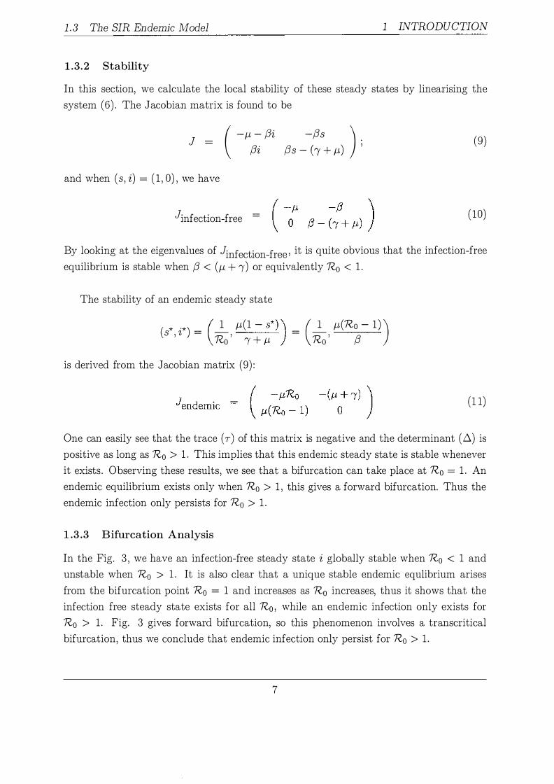
1.3.2 Stability
In this section, we calculate the local stability of these steady states by linearising the
system (6) . The Jacobian matrix is found to be
J
and when (s , i) = (1, 0) , we have
( -M - (3i (3i
]infection-free =
-(3s ) (3s - h+ M) ' (9)
(10)
By looking at the eigenvalues of ]infection-free ' it is quite obvious that the infection-free
equilibrium is stable when (3 < (M + 1) or equivalently R0 < 1.
The stability of an endemic steady state
(s* , i*) = (J_, M(1 - s*))
= (J_, M(Ro - 1) )
Ro 1 + M Ro (3
is derived from the Jacobian matrix (9) :
(11)
One can easily see that the trace ( T) of this matrix is negative and the determinant ( 6.) is
positive as long as R0 > 1. This implies that this endemic steady state is stable whenever
it exists . Observing these results , we see that a bifurcation can take place at R0 = 1. An
endemic equilibrium exists only when R0 > 1, this gives a forward bifurcation. Thus the
endemic infection only persists for R0 > 1.
1.3.3 Bifurcation Analysis
In the Fig. 3 , we have an infection-free steady state i globally stable when R0 < 1 and
unstable when R0 > 1. It is also clear that a unique stable endemic equlibrium arises
from the bifurcation point R0 = 1 and increases as R0 increases, thus it shows that the
infection free steady state exists for all 7?0 , while an endemic infection only exists for
R0 > 1. Fig. 3 gives forward bifurcation, so this phenomenon involves a transcritical
bifurcation, thus we conclude that endemic infection only persist for R0 > 1.
7

1 . 3 The SIR Endemic Model 1 INTRODUCTION
0.04
0.03-
0.02-
0.01
0 1------------'--------------------------------
·0.01 --·----"----····--··--L......_-...L.---L... ... _______ c __ ___, ____ J.......... ____ _ 0.8 0.85 0.9 0.95 1 1.05 1.1 1.15 1.2 Ro
Figure 3 : Bifurcation analysis for SIR endemic model. Stable infection-free steady state for R0 < 1 ; unstable infection-free i and stable endemic steady state i* for R0 > 1 .
1.3.4 Phase-Plane Analysis
We analyse equations of the system (6) , in the (s, i) phase-plane, for different values of
R0 (see Fig. 4) . The arrows represent the direction of solutions and a dark black dot
represents the equilibrium point. Dashed lines show nullclines and the dark black line
shows the triangle X. Some plotted curves show solutions of system (6) . Observe that
the qualitative behaviour changes at R0 = 1 .
• If R0 < 1 : The infection-free steady state is globally asymptotically stable i .e .
globally attracting and biologically feasible endemic solutions do not exist in Fig. 4
(a) .
• If R0 > 1 : The infection-free steady state is unstable and a unique endemic equi
librium exists, and is globally asymptotically stable in Fig. 4 (b) .
1.3.5 Summary
In this section we have shown that if R0 > 1 , then an epidemic will occur. We have also
proved that, biologically, an endemic infection can only continue to exist in a population
for R0 > 1 . Hence, we conclude that for R0 < 1 , the infection-free equilibrium is globally
attracting, this means that if the average number of secondary infections caused by an
8

1 . 3 The SIR Endemic Model 1 INTRODUCTION
���------------------.-�b�--.------------------=--. f•C�·G.tlS�!·C!ll t'"!#•2s!tn•sl·U n=e� i':rC!.t5ti·i�H I ·� . I "' 1 Ut· ! C?� 11�
i -Hr ''f llf ul I lif
i --:��"·,_,__:;:::::::;::::::§���__;.�\_,� li······· i ' I U U U U U H U U U I
1'=2s!t='�s/·H·Hgj J=Oti
0 u " u u " u u u u 1
__ _,__ _____ .L_ ________ ___,_, __________ _j
Figure 4: Phase-Plane for SIR endemic model when: (a) R0 = 0 .5 < 1 ; (b) R0 = 2 > 1 . Other parameter values are p, = 0.02 and 1 = 0 .05 .
infective is less than one, then the infection will no longer persist . If R0 > 1 , then the
infection-free steady state is unstable. Thus the endemic steady state (s* , i* ) is globally
attracting only for R0 > 1 .
In the following chapter we will consider four extensions of the SIR endemic models.
These four models have an endemic infection that persists for some values of Ro < 1
(which are close enough to one) that leads to phenomena of backward bifurcation, multiple
endemic steady states and hysteresis.
9

2 2D EXTENSIONS
2 2D Extensions In this chapter, we will study four extensions of SIR endemic models, their potential for
a backward bifurcation and the presence of sub-critical endemic steady states. We will
also examine the dynamics of these models by varying parameters values.
In these models an endemic infection is maintained in the population when R0 > 1 and
when R0 equals certain values less than one. The main bifurcation parameter R0 is also
considered as a fundamental epidemiological parameter; while P, as mentioned previously,
is a secondary parameter, whose definition varies between the different models.
2 .1 The SIR model with Susceptible R Class
In this model, the recovered R class is susceptible, and possibly even more susceptible, to
infection than the susceptible class, as examined in the paper by Safan et al. [13] . This
model has been used for treatment effects in case of tuberculosis; the infective class in a
population is treated at a constant rate and then proceeds to a recovered class, described
as treatment T in Feng et al. [4] . The system of differential equations is
J-l-j3si-J-lS, ds dt di dt - j3si + P j3ri -(J-l + 1 )i. (12)
with r(t) = 1 - s(t) -i(t). The parameters /3, J-l, 1 and R0 = +!3 are as in Sect . 1 . The I J-L parameter P is defined as the ratio of transmission probabilities from the recovered and
susceptible classes. In this model, if P = 0 , then we have the SIR model, in which the
population has zero susceptibility after recovering from one infection; and if P = 1 , then
we have the SIS model, in which the infected class returns to the susceptible class on
removal or recovery, see [13] .
In a similar manner to Sect . 1 . 3 , we calculate the global stability of the steady states
by applying the classical Poincare-Bendixson theorem. Periodic solutions are ruled out
using Dulac's criterion in (s, i) E X region. Here d(�;i) = Pj3ri- 1i = -1i < 0 when
s + i = 1 and r(t) = 0 , thus any trajectory that starts in X stays in X. � (J-l-j3s�-J-lS)
+ � (Pj3ri-:i-J-li) = _ _!!__ _ _
Pj3 < O. 8s S'l 8z S'l s2z S (13)
Equation ( 13) implies that this model does not have any limit cycles in the region X, thus
10

2. 1 The SIR model with Susceptible R Class 2 2D EXTENSIONS
the steady state for R0 > 1 is globally stable if it exists .
2.1.1 Steady State Solutions
We begin a qualitative approach to study steady states solutions. In order to get the
equilibrium condition, we set the right hand side of equations in the system (12) to
zero. By factorising these equation we find that the infection-free equilibrium occurs at
(s , i) = (1, 0) .
The endemic condition satisfies f]s + P/3(1 - s - i) - (J + J-t) = 0 . Now, we have two
types for endemic steady states: P = 0 ; and P =f. 0 . For P = 0 the endemic steady states
are ( s* , i*) = ( �0, J.L(R�-l) ) , as in Sect. 1.3 .1. If P =f. 0, then we find the endemic steady
states for s* = J.L4i* where i* is found by solving the quadratic equation
f (i*) = PR0i*2+(1+Pf - PRo) i*+f (�0
- 1) = 0 , (14)
where r = J.L�I'· If R0 > 1 and P > 0 , then f(O) < 0 and there is a unique positive
solution i* > 0 with j(i*) = 0. For R0 < 1, we need to solve equations (14) to have better
understanding of the roots for j(i*) . We have
.* 1 (-1 - Pr +PRo)± Ju + Pr - PRo)2 - 4Pr (1 - Ro) z±
= 2 PRo
We consider the discriminant of f (i*) when R0 < 1, we have three possibilities for the
solutions of f(i*) : if the discriminant of j(i*) is negative, then we have no real roots; if
the discriminant of f (i*) is positive, then we have two real roots; and if the discriminant
of j(i*) is zero, then we have one real root . Graphically, the parabola of j(i*) is concave
up and is tangential to the i*-axis whenever R0 = Rsaddle and if R0 > Rsaddle ' then
the parabola intersects the i*-axis. There is still another situation to consider, which
characterises the critical or turning points for P and R0.
2.1.2 Saddle Node Equation
The following is an elaborate from equation (14) to obtain the critical value for P. For
this treating R0 as a function of i* and differentiating equation (14) . Hence we get
.* PRo - Pr - 1 z = ------2RoP
11

2. 1 The SIR model with Susceptible R Class 2 2D EXTENSIONS
f-L 0.02 I 0.05 r 0.286
Rsaddle 0 .871699
Pcrit 1 . 4
Table 2 : Parameter values for susceptible R class.
at the critical point we obtain ��0 I (l,o) = Jl.�l P - 1 . This gives
h dRol - 0 w en di* (I,o) - ·
f-L Pcrit = 1 + I
Now decreasing R0 on the horizontal axis in order to find the saddle node equation
for R0 when P > Pcrit · Putting this value of i* back into equation ( 14) , the saddle node
solution, for the value of R0 , becomes
P2R6 + ( (2 - P)r - 1) 2PRo + ( 1 - Pf)2 = 0.
The solution of this equation gives Rsaddle ' the value of R0 where two endemic steady
states with i-component i_ = i+ = i* coincide in the turning point (see Fig. 5) only
when P > Pcrit · For more details see [13] .
2.1.3 Stability
In this subsection, we investigate the stability of these steady states by linearising equa
tion ( 12) . The Jacobian matrix for this model is
J ( -p,- (3i -(3s ) (3i ( 1 - P) (3s + P/3(1 - s - 2i ) - (p, + 1) . ( 15)
At the infection-free steady state, (s, i) = ( 1 , 0) , we have a Jacobian matrix as in ma
trix (10) , and from which we have already found that if R0 < 1 , then an infection-free
equilibrium is locally stable for all values of P. If R0 > 1 , then we have an unstable
infection-free equilibrium.
Using the endemic steady state for s* and i* , when P = 0 , the matrix ( 15) becomes
matrix ( 1 1 ) . When R0 > 1, we have T < 0 and 6. > 0, thus the endemic steady state is
stable for P = 0 .
12
2. 1 The SIR model with Susceptible R Class 2 2D EXTENSIONS
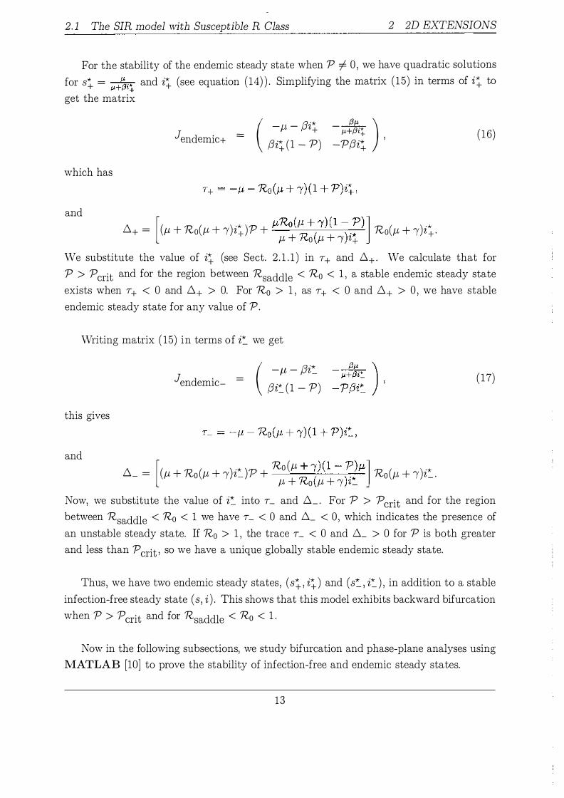
For the stability of the endemic steady state when P =/= 0 , we have quadratic solutions
for s� = p,�i+ and i� (see equation (14) ) . Simplifying the matrix (15) in terms of i� to
get the matrix
which has
and
J -f.L - '/,+ - p,+(3i* ( j3 "* (3p, ) endemic+ =
/3i�(1 - P) -P/3ii '
,6.+ = [ (J.L + Ro(J.L + !)i�)P + J.LRo (�+
(l) ( 1 )·:')] Ro(J.L + !)i�. f.L + o f.L + 1 z+
( 16)
We substitute the value of i� (see Sect. 2 . 1 . 1 ) in T+ and ,6.+ · We calculate that for
P > P crit and for the region between Rsaddle < R0 < 1 , a stable endemic steady state
exists when T+ < 0 and ,6.+ > 0. For R0 > 1 , as T+ < 0 and ,6.+ > 0 , we have stable
endemic steady state for any value of P.
Writing matrix ( 15) in terms of i=_ we get
this gives
and
-j.L- '/,_ ( /3"* J . -endemic- -j]i=_ ( 1 _ P)
,6._ = [(J.L + Ro (J.L + !)i=-_)p + Ro (J.L � �) ( 1 -;.lf.L] Ro(J.L + !)i=-_.
J.L + 0 J.L +! z_
( 17)
Now, we substitute the value of i=-_ into L and ,6._ . For P > 'Pcrit and for the region
between Rsaddle < R0 < 1 we have L < 0 and ,6._ < 0 , which indicates the presence of
an unstable steady state. If R0 > 1 , the trace L < 0 and ,6._ > 0 for P is both greater
and less than P crit , so we have a unique globally stable endemic steady state.
Thus, we have two endemic steady states , (s�, i�) and (s=-_, i=-_) , in addition to a stable
infection-free steady state ( s, i ) . This shows that this model exhibits backward bifurcation
when P > 'Pcrit and for Rsaddle < Ro < 1 .
Now in the following subsections, we study bifurcation and phase-plane analyses using
MATLAB [10] to prove the stability of infection-free and endemic steady states.
13
2. 1 The SIR model with Susceptible R Class
s* , , 0.8 , I I
...... ,.,. '' ,
p = pcrlt··· ....... ,
0.6
0.4
P:Pcrll 0.2
...
i* ·········
.... ··········
0.8 0.85 0.9 0.95 1.05
······ ... ... ...
······ ·····
····· .... ····· ...
1.1 1.15
2 2D EXTENSIONS
1.2
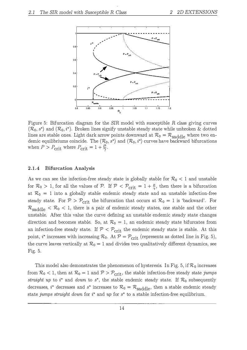
Figure 5 : Bifurcation diagram for the SIR model with susceptible R class giving curves (R0 , s*) and (R0 , i*) . Broken lines signify unstable steady state while unbroken & dotted lines are stable ones. Light dark arrow points downward at R0 = Rsaddle where two endemic equilibriums coincide. The (R0 , s*) and (R0 , i*) curves have backward bifurcations when P > Pcrit where Pcrit = 1 + �. 2.1.4 Bifurcation Analysis
As we can see the infection-free steady state is globally stable for R0 < 1 and unstable
for Ro > 1 , for all the values of P. If P < Pcrit = 1 + �' then there is a bifurcation
at R0 = 1 into a globally stable endemic steady state and an unstable infection-free
steady state. For P > Pcrit the bifurcation that occurs at R0 = 1 is 'backward' . For
Rsaddle < Ro < 1 , there is a pair of endemic steady states, one stable and the other
unstable. After this value the curve defining an unstable endemic steady state changes
direction and becomes stable. So, at R0 = 1 , an endemic steady state bifurcates from
an infection-free steady state. If P < Pcrit the endemic steady state is stable. At this
point , i* increases with increasing Ro . At P = Pcrit (represents as dotted line in Fig. 5) ,
the curve leaves vertically at R0 = 1 and divides two qualitatively different dynamics, see
Fig. 5 .
This model also demonstrates the phenomenon of hysteresis. In Fig. 5 , i f R0 increases
from Ro < 1 , then at Ro = 1 and P > P crit , the stable infection-free steady state jump s straight up to i* and down to s* , the stable endemic steady state. If R0 subsequently
decreases, i* decreases and s* increases to R0 = Rsaddle , then a stable endemic steady
state jump s straight down for i* and up for s* to a stable infection-free equilibrium.
14
2. 1 The SIR model with Susceptible R Class
$':t0DZ·�t$.'"9Si-O.o2s l'•�W."1tl·O,C1l
2 2D EXTENSIONS
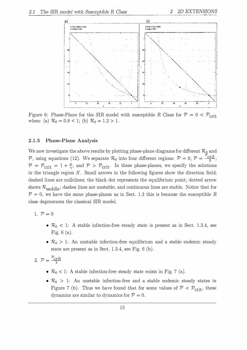
Figure 6 : Phase-Plane for the SIR model with susceptible R Class for P = 0 < Pcrit when: (a) Ro = 0 .8 < 1 ; (b) R0 = 1 . 2 > 1 .
2.1.5 Phase-Plane Analysis
We now investigate the above results by plotting phase-plane diagrams for different R0 and p 0
P, using equations ( 12) . We separate R0 into four different regions: P = 0 ; P = �; P = Pcrit = 1 + �; and P > Pcrit· In these phase-planes, we specify the solutions
in the triangle region X. Small arrows in the following figures show the direction field;
dashed lines are nullclines; the black dot represents the equilibrium point; dotted arrow
shows Rsaddle ; dashes lines are unstable ; and continuous lines are stable. Notice that for
P = 0 , we have the same phase-planes as in Sect . 1 . 3 this is because the susceptible R class degenerates the classical SIR model.
1 . p = 0
• R0 < 1 : A stable infection-free steady state is present as in Sect . 1 . 3 .4 , see
Fig. 6 (a) .
• R0 > 1 : An unstable infection-free equilibrium and a stable endemic steady
state are present as in Sect . 1 . 3 .4 , see Fig. 6 (b) .
� 2. p = 2 • R0 < 1 : A stable infection-free steady state exists in Fig. 7 (a) .
• R0 > 1 : An unstable infection-free and a stable endemic steady states m
Figure 7 (b) . Thus we have found that for some values of P < Pcrit ' these
dynamics are similar to dynamics for P = 0 .
15

2. 1 The SIR model with Susceptible R Class
a S''"l!li·RO\m+�}s-l•tm1 �:t\l02' s-.J=C.� t':r::RC{J:U�gt:"MW}SitPR$�+�){1·S·�l·{l'WfSfzrA}i R:JaU p:0,1
2 2D EXTENSIONS
b S'"'Wll·f!.'O(a.tt�H·�:t I!U10.Dl �eo,� i':rP.G{tw.J�'I+PRtl(nH)W"Jii.1+QHJW+�':'t',.,Ji f\?:;1.2 {1:0..7
� Figure 7: Phase-Planes for susceptible R class for P = 2 when: (a) 7?0 = 0 .8 < 1 ; (b) Ro = 1 . 2 > 1 .
a) S't0.�·�S:I•G02t !'1:Q�,:l+SC$$2i(1·S·ill·0Ut
l _______ 0.1 ----
b) J1:am·RO(w+gn:e�HI�r14t !':rR3{1Wt��lt,Rjft:Jt�(t+bl·tnJ+�I
Figure 8 : Phase-Planes for susceptible R class for P = Pcrit when: (a) 7?0 = 0 .8 < 1 ; (b) 'Ro = 2 > 1 .
16

2. 1 The SIR model with Susceptible R Class
b
2 2D EXTENSIONS
s'•O.ti·0�1Rfsi·V.Dl"s i'-=DJTfQ tl+P"�e7 R:Ott· s-�1· M1 1
Figure 9 : Phase-Planes for susceptible R class for P = 2 .8 > Pcrit when: (a) R0 = 0 .5 < Rsaddle ; (b) Ro = 'Rsaddle ·
a) ;':tODJ•00$.4U·M2t l'•�.�liH1Sf,tki·9l•Uil
b)
Ql
t•!<Q!I1·C.1l$f•O.Vl-s I'•C.Utit05i-(1•s.·�l·O�t!
Figure 10 : Phase-Planes for susceptible R class for P = 2 .8 > Pcrit when: (a) Rsaddle < Ro = 0.92 < 1 ; (b) R0 = 2 .
17

2.2 The SIR model with Nonlinear Transmission Class 2 2D EXTENSIONS
3 . P = Pcrit
• R0 < 1 : Only a stable infection-free equilibrium is present in Fig. 8 (a) • R0 > 1 : An unstable infection-free steady state and stable endemic steady
states are present in Fig 8 (b) .
4 . P > Pcrit
• Ro < Rsaddle : Only a stable infection-free equilibrium is present in Fig. 9 (a) .
• Ro = Rsaddle = 0 .871699: A stable infection-free steady state exists. Another
equilibrium point shows two endemic steady states which are top of each other
at this value of Rsaddle· The nullclines are tangential to each other.
• Rsaddle < Ro < 1 : An stable infection-free, two endemic both stable and
unstable exist in Fig. 10 (a) .
• R0 > 1 : An unstable infection-free steady state and one stable endemic steady
state are present in Fig. 10 (b) .
2 .2 The SIR model with Nonlinear Transmission Class
The SIR model with nonlinear transmission of infection is explained in detail in Comes et
al. [6] . In this model, we show that the transmission function of any infection satisfies the
biological conditions that lead to the system with an asymptotically stable steady state
[8] . The differential equations are written as
ds dt di dt
J-L - AS - f-LS, ( 18 )
AS - (J-L + !)i .
with r (t) = 1 - s (t)- i(t) as above. Take A = f3i (1 + h(i)) as a nonlinear force of infection
for some increasing function h. This function h( i) is defined as the increase in risk of
infection with the intensity of exposure, and if h(i) _ 0 , then we have a standard force
of infection A = f3i as analysed in [6] . We have assumed that h' (i) ;:::: 0. Thus considering
h(i) using a functional form h(i) = 1;�i in order to get useful illustrations; here we use
P as a secondary bifurcation parameter. The basic reproduction number R0 = f-l � 1 is
unchanged.
In order to find the global stability, we consider the triangle X as an invariant set
such that X= { s, i E R2l(s, i) > 0 ; (s + i :::; 1) }, then d(�-;-i) = J-L - J-L(s + i) - 1i < 0 when
s + i = 1 . We use Dulac's criterion [2] that states that if the sign of �! + �� is constant
18

2.2 The SIR model with Nonlinear Transmission Class 2 2D EXTENSIONS
in a simply connected region X, of the phase space, then limit cycles cannot exist in the
region. !!_ (f-L- AS- f-LS) � (AS - ,i - fJ,i) = _j!_ P/3
os si +
oi si s2i +
( 1 + Pi)2 ( 19 )
As the above expression changes sign in the region X , by using Dulac's criterion and
the Poincare-Bendixson theorem. Thus, we cannot exclude limit cycles and cannot say if
the non trivial steady state is globally asymptotically stable for the function h( i) = 1:�i. Thus, any conclusion about the existence of limit cycle, cannot be drawn and, in this case
Dulac's criterion fails.
Note that in some cases , we do not apply Dulac's criterion to this model, as there are
some functions h( i) that may lead to limit cycles surrounding the nontrivial equilibrium,
as demonstrated in Games et al. [6). Games provide a theorem stating that there may
exist at least one limit cycle derivable from the function h( i ) . Correspondingly if h" ( i ) < 0
and h" ( i) > 0 , then we have at least one limit cycle surrounding the equilibrium provided
h' (O) < (J.L�'Y) and h"(O) > Sl(�:'Y) - 3h'(O�J.L+'Y) .
We apply this theorem for the function h(i) 1:�i· If h'(O) = P < (J.L�'Y) , then
h"(O) < Sl (J.L+'Y) - 3h' (o)(J.L+'Y) • and if h' (O) = P > (J.L+'Y) then h"(O) > Sl (J.L+'Y) - 3h' (O) (J.L+'Y) 4j.L J.L ' J.L ' 4J.L J.L '
this shows that this theorem fails. This theorem is helpful if any limit cycle exists for
the function h(i) , however, the theorem does not say what happens if this theorem fails.
Thus the nonexistence of any limit cycles for any value of the parameter P, when 1?0 > 1
remains in question.
2.2.1 Steady State Solutions
A steady state can be found by solving the system (18) , with the right hand sides set to
zero. f-L - /3(1 + h( i) ) si - f-LS = 0,
/3(1 + h(i) ) si - (J-L + !)i = 0.
We get an infection-free equilibrium at (s , i) = ( 1 , 0) as in Sect . 2 . 1 . For all P , the endemic
steady state is the solution of:
s* -
1
1 Ro ( 1 + h(i* ) ) '
1 (J-L +!)i* R0 ( 1 +h(i*) )
+ {t
19
(20)
(21 )
2.2 The SIR model with Nonlinear Transmission Class 2 2D EXTENSIONS
We may find either a unique positive solution or multiple solutions for equation ( 21) , depending on the function h(i ) . Now, if P = 0 , then we have the same endemic steady
state as in Sect. 2 .1. And for any other values for P, we have endemic steady states for
i* and s* . We solve equation (21) in quadratic form, using h(i) = 1:�i·
j(i*) = 2PR0i2* + (Ro - 2PR0f + Pr)i* + f(1 - Ro) = 0 ,
* 1 + Pi*
s = --;------:-Ro(1 + 2Pi*) '
(22)
where r = J.L�1 as in Sect . 2 .1. For the function h(i) = 1:�i ' we find that f (i*) has a
unique positive solution i* > 0 for j(O) < 0 whenever R0 > 1. But if R0 < 1, then we
have a more complex situation so in order to get a better analysis, we solve equation (22) to get
.*
1 (2PRof - Ro - Pf) ± -j(Ro - 2PR0f + Pf)2 - 8PR0f(1 - R0) '/,± = 4 PRo
Whenever R0 < 1, we have three possibilities for the solutions of f(i*) . If the discriminant
of f (i*) is positive then we have two real roots and if negative then we have no real roots.
If it is zero then graphically, we have a concave up parabola of j( i*) which is tangential
to the i* -axis. At this point we have Rsaddle that makes the parabola tangential on the
i*-axis.
In the following subsection, we will calculate the critical values for P and RsaddleAlso we analyse the turning points where the backward bifurcation occurs.
2.2.2 Saddle Node Equation
To determine the direction of bifurcation at the critical point , we solve equation (21) treating R0 as a function of i* , giving a value for
.*
2PRor - Ro - Pr z = 4PRo .
If We Set 'Do = 1, " * - 0 then dRo I - i:!:_±J_ - h' (0) As dRo < 0 thus ''"' 0 - ) di* (1,0) - f-L . di* - )
h' (O) > Pcrit = 1 + J... f-L
20

2.2 The SIR model with Nonlinear Transmission Class 2 2D EXTENSIONS
j}, 0.02 'Y 0.05 r 0 .286
Rsaddle 0.9519197 P(:rit 3 .5
Table 3 : Parameter values for nonlinear transmission class.
This gives the critical value of Pcrit and for P > Pcrit ' we calculate the saddle node
equation for R0 . Putting the value of i* back into equation (22) to get
This equation solves for the value of Rsaddle· Thus, when P > Pcrit and Rsaddle < R0 < 1 , a backward bifurcation occurs. We will calculate the stability of infection-free
and endemic steady states in next subsection.
2.2.3 Stability
We linearise the system (18) in order to study stability of these steady states. The
Jacobian matrix is given by
J = ( -f.J, - j3i(1 + h(i) ) -j3s(1 + ih' (i) + h(i) ) ) (23)
j3i( 1 + h(i)) j3s(1 + ih' (i) + h(i)) - (J-l + 'Y) ·
For the infection-free steady state (s , i) = ( 1 , 0) , this Jacobian matrix is the same as
the matrix (10) . Thus, for R0 < 1 , (s , i) = ( 1 , 0) is stable and; for R0 > 1 , it is
unstable. To study the stability of the endemic steady state for P = 0, we set (s* , i*) = ( io , J-l(R�- 1) ) . The Jacobian matrix (24) is same as the matrix ( 11 ) and possess the
same stability for R0 > 1 i .e . we have stable endemic steady state for R0 > 1 for the
parameter values given in Table 3 .
When P =J. 0, we have the endemic steady states (see equations (20) ) , (21 ) ) . We find
the Jacobian matrix and solve it for the function h(i* ) . Thus we have
(24)
21
2.2 The SIR model with Nonlinear Transmission Class 2 2D EXTENSIONS
with Roi� (p, + 1) (1 + 2Pi�) (p, + !)Pi�
T+ = -p, - 1 + Pi� + (1 + Pi+ ) (1 + 2Pi+) '
and determinant
6 = (p, + !)i� [4Roi�P2 (p, + !) + 4Roi�P(p, + !) + R0 (p, + !) - p,P]
+ ( 1 + 2Pi+ ) ( 1 + Pi+) .
Substituting the value of i� and the parameter values from Table 3 in T+ and 6+ to evaluate ]endemic+ (24) . We find that for P > Pcrit and Rsaddle < R0 < 1 , a stable endemic steady state i� exists. For R0 > 1 , we have only one stable endemic steady state
as ]endemic+ (24) has only real negative eigenvalue for any P.
Putting the endemic steady state i:_ in the matrix (23) to get
We get
and
]endemic-
(J.t+Y)(1+4Pi::_ +2P2i::_2) (l+Pi::_) (l+2Pi::_ ) (J.t+'Y)Pi::_
R0i:_ (p, + 1) (1 + 2Pi:_ ) (p, + !)Pi:_ r_ = -p, - 1 + Pi� + ( 1 + Pi� ) ( 1 + 2Pi� ) '
6 = (p, + !)i-:_ [4Roi:_P2 (p, + !) + 4Roi:_P(p, + !) + R0 (p, + 1) - p,P]
- (1 + 2Pi� ) (1 + Pi� )
(25)
By substituting i:_ into L and 6_ , we find that L < 0 and 6_ < 0 whenever P > P crit and Rsaddle < Ro < 1 , hence an unstable endemic steady state i:_ exists. Additionally,
if R0 > 1 , then we have stable endemic steady states for any P. Thus, for P > Pcrit and
Rsaddle < Ro < 1 , we have multiple endemic steady states.
2.2.4 Bifurcation Analysis
The dynamics of this system are similar to those of the susceptible R class described in
the previous Sect . 2 . 1 . So for the bifurcation analysis we refer the read to that Sect. 2 . 1 . Fig. 1 1 illustrates same dynamics as Fig. 5 that a backward bifurcation occurs at R0 = 1 , this refers to sub-critical endemic steady states (shown as dashed and solid black lines) and a stable infection-free equilibrium.
2.2.5 Phase-Plane Analysis
In this section, we analyse the system (18) using a (s, i) phase-plane, the methodology
is similar to that of Sect . 2 . 1 . We find the force of infection (>.) by calculating the
22

2.2 The SIR model with Nonlinear Transmission Class 2 2D EXTENSIONS
- - - - - - - - - - - - - - - -.. .. .. .. .. P < PerU , . . . · ·
· · · ·
s * . . . · · ·· ·
' • • . . . . . . , , , P = pcrit 0.8 · · · · ·
0.6 \ 0.4 P > P er it
0.2 I i* - - - · · · · · · · · · · · · · · · · · · · · · · · · · · · · · · · · · · · · · · · · · · · · ·
·
0 - - - - - - - - - - -R saddle
0.9 0.92 0.94 0.96 0.98 1 .02 1 .04 1.06 1 .08 1 . 1 Ro
Figure 1 1 : Bifurcation diagram for the SIR model with nonlinear transmission class. Labels are as in Fig. 5. For this class, P crit = 1 + �.
function h( i) = (l:�i) to plot the phase-planes. We have plotted several phase-planes by
categorising R0 in different regions and using different values for P.
1 . P = 0 < P crit
• R0 < 1 : A stable infection-free steady state (s , i) = ( 1 , 0) exists in Fig. 1 2 (a) .
• R0 > 1 : An unstable infection-free and a stable endemic steady states exist in
Fig. 12 (b) .
P = � 2 . 2
• Ro < 1 : A stable infection-free steady state exists in Fig. 13 (a) .
• Ro > 1 : An unstable infection-free and a stable endemic steady states exist in
Fig. 13 (b) .
3. P = Pcrit
• R0 < 1 : A stable infection-free steady state is present in Fig. 14 (a) .
• Ro > 1 : An unstable infection-free steady state and a stable (spiral sink)
endemic steady state (s* , i*) are present in Fig. 14 (b) .
4· P > Pcrit
23

2.2 The SIR model with Nonlinear Transmission Class
a ) b)
2 2D EXTENSIONS
t'"'N-R0�-f�}Sf(1+lPQ!:,l +P�·M.it !I'V110A2 PJ•GJ :s'sr.u.f*,«.�•S£tVJJ!(I+ 2P(Al +PO·�t v,p:Qel �:r.t.t i':r:�C:u+�tlt1+2Pf'A1 +?4•tm:.�+;ur.4:H �*OM P<l i'"'�t.t\l+�sl{J+ZP�ttPij·(r'c+�i �s-0.05 P•$
J- I , ,
I I J J ur I j I I J .. l I I I I ! -�'I I I l Hr !
.,� _J Oll I ·I ! �� tl M H u Ol OJ 0.1
Figure 12: Phase-Planes for the SIR model with nonlinear transmission class for P = 0 < Pcrit when: (a) Ro = 0 .8 < 1 ; (b) R0 = 1 . 2 > 1 .
a ) b) �--------------------------�-----------------------------� l'•ro·�\IN.l+�sl(tt1Jit�t tP�·:wS tt�"C� �·dOS �'•t%1•P.I�•�d(1+1P�!1-P1Nffl t eqsCO� �t•DM 1'011i:�tru+�J)ti0+2Pf41 •1-'Q·�+�)' P "' ln Ra,...o.t l'=fQ�-o-p;:w�)d(t+2PIJ1_1tPO·Qm:+�JI �"115 Rl"'l.l
Figure 13 : Phase-Planes for nonlinear transmission class for P 0 .8 < 1 ; (b) R0 = 1 . 2 > 1 .
24
p . .::.q:tt when: (a) R0
2.2 The SIR model with Nonlinear Transmission Class 2 2D EXTENSIONS
a ) S' .. �·PiOtrtJt�}SitfHP�l�P�·mU l'!:�im:•�titl tl?�t-tP$-In.�tgrr�i
01
.m•OQ? Jtl•O.t -·IM P•l.!
b) t'*'W·Iltltrut�ti{l +l.P� H�-m:s i':=fi:}!!V.It;am"M}tl(t+lPI;\t•Pl)·(ltolt�J
rw•C-Ot rtl$'t� �=�� ?=U
Figure 14: Phase-Planes for nonlinear transmission class for P R0 = 0. 8 < 1 ; (b) R0 = 1 . 2 > 1 .
3 .5 = Pcrit when: (a)
aJ
t'"WJ·a3(mlt�$1{l tlP�lt?IJ·rnU J't�fro�t�'ltt•1P�t.;.?9·(W+�H
!'l\lt"GC'2 no.-o.s ;UtJtA=-O.C'!. P::1
b) s' .. O.Ol·G�1�si(tHp�t•;�·e�s l'•O:HR.4Sl(t i"lpit\fiplj·QD11
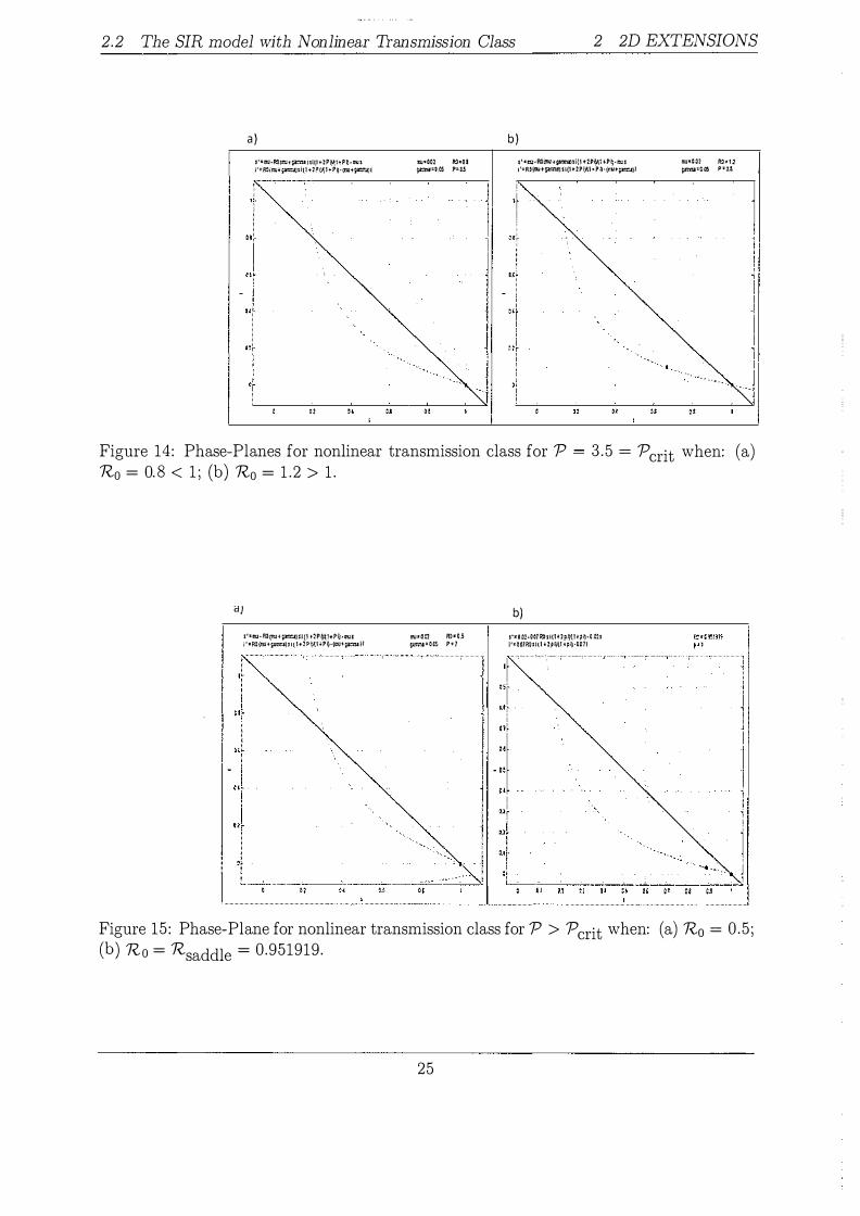
Figure 15 : Phase-Plane for nonlinear transmission class for P > Pcrit when: (a) R0 = 0 .5 ; (b) Ro = Rsaddle = 0.951919 .
25
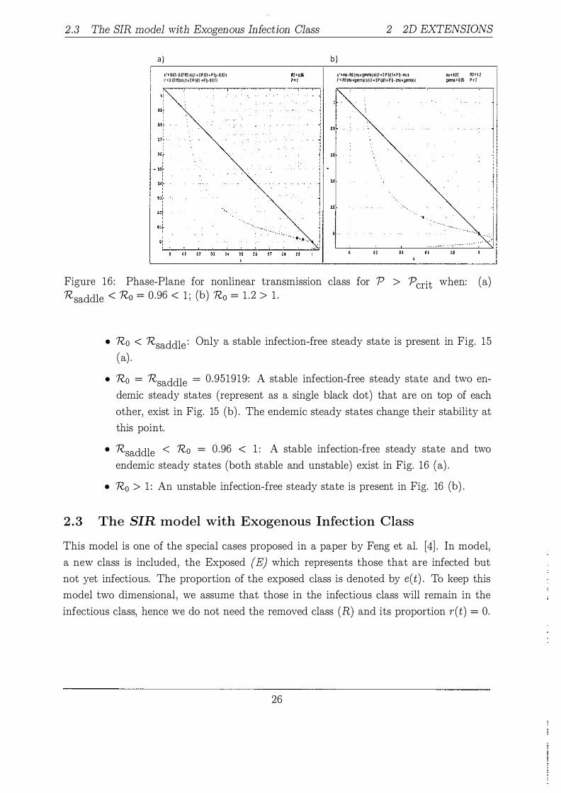
2.3 The SIR model with Exogenous Infection Class 2 2D EXTENSIONS
a) s•: 002· 0,07 RJs l(f 1-2?\11 +P �·G.� i i'::: am��lttiZPi;\1 -tP�·OVil
b ) i'=tti•Rll (::W+�}ll(l i�P�I-J?�·m.JS i''i\!{lllifl'"''lliii+2Pij\11PI·""'-}I
WJ0,01 JU1'Jl ;gm::: OJIS ? :1
Figure 16 : Phase-Plane for nonlinear transmission class for P > 'Pcrit when: (a) Rsaddle < Ro = 0.96 < 1 ; (b) 1?0 = 1 . 2 > 1 .
• Ro < Rsaddle : Only a stable infection-free steady state is present in Fig. 15 (a) .
• Ro = Rsaddle = 0.951919 : A stable infection-free steady state and two en
demic steady states (represent as a single black dot) that are on top of each
other, exist in Fig. 15 (b) . The endemic steady states change their stability at
this point.
• Rsaddle < Ro = 0.96 < 1 : A stable infection-free steady state and two
endemic steady states (both stable and unstable) exist in Fig. 16 (a) .
• R0 > 1 : An unstable infection-free steady state is present in Fig. 16 (b) .
2 . 3 The SIR model with Exogenous Infection Class
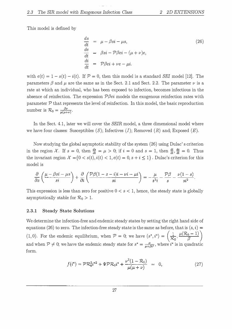
This model is one of the special cases proposed in a paper by Feng et al. [4] . In model,
a new class is included, the Exposed (E) which represents those that are infected but
not yet infectious. The proportion of the exposed class is denoted by e(t) . To keep this
model two dimensional , we assume that those in the infectious class will remain in the
infectious class, hence we do not need the removed class (R) and its proportion r(t) = 0.
26
2.3 The SIR model with Exogenous Infection Class
This model is defined by
ds dt de dt di dt
f-L - (3si - f-LS, f3si - P(3ei - (f-L + v)e,
P f3ei + ve - f_Li.
2 2D EXTENSIONS
(26)
with e(t) = 1 - s (t) - i (t) . If P = 0, then this model is a standard SEI model [12] . The
parameters f3 and f-L are the same as in the Sect. 2 . 1 and Sect . 2 .2 . The parameter v is a
rate at which an individual, who has been exposed to infection, becomes infectious in the
absence of reinfection. The expression P f3ei models the exogenous reinfection rates with
parameter P that represents the level of reinfection. In this model, the basic reproduction
b . R - (3v num er IS o - p,(J.L+v) .
In the Sect. 4. 1 , later we will cover the SEIR model, a three dimensional model where
we have four classes: Susceptibles (S) ; Infectives (I) ; Removed (R) and; Exposed (E) .
Now studying the global asymptotic stability of the system (26) using Dulac' s criterion
in the region X. If s = 0, then �� = f-L > 0; if i = 0 and s = 1 , then � ' �� = 0. Thus
the invariant region X ={0 < s (t) , i (t) < 1 , e(t) = 0, s + i ::; 1 } . Dulac's criterion for this
model is
This expression is less than zero for positive 0 < s < 1 , hence, the steady state is globally
asymptotically stable for R0 > 1 .
2.3.1 Steady State Solutions
We determine the infection-free and endemic steady states by setting the right hand side of
equations (26) to zero. The infection-free steady state is the same as before, that is (s, i) =
( 1 , 0) . For the endemic equilibrium, when P = 0; we have (s* , i*) = ( io , 1-L (R�- 1 ) ) and when P =/= 0; we have the endemic steady state for s* = �, where i* is in quadratic
form.
(27)
27
2.3 The SIR model with Exogenous Infection Class
f-l 0 .02 l/ 0 .05
nsaddle 0 .9838 Pc.rit 8 .75
2 2D EXTENSIONS
Table 4: Parameter values for exogenous infection class.
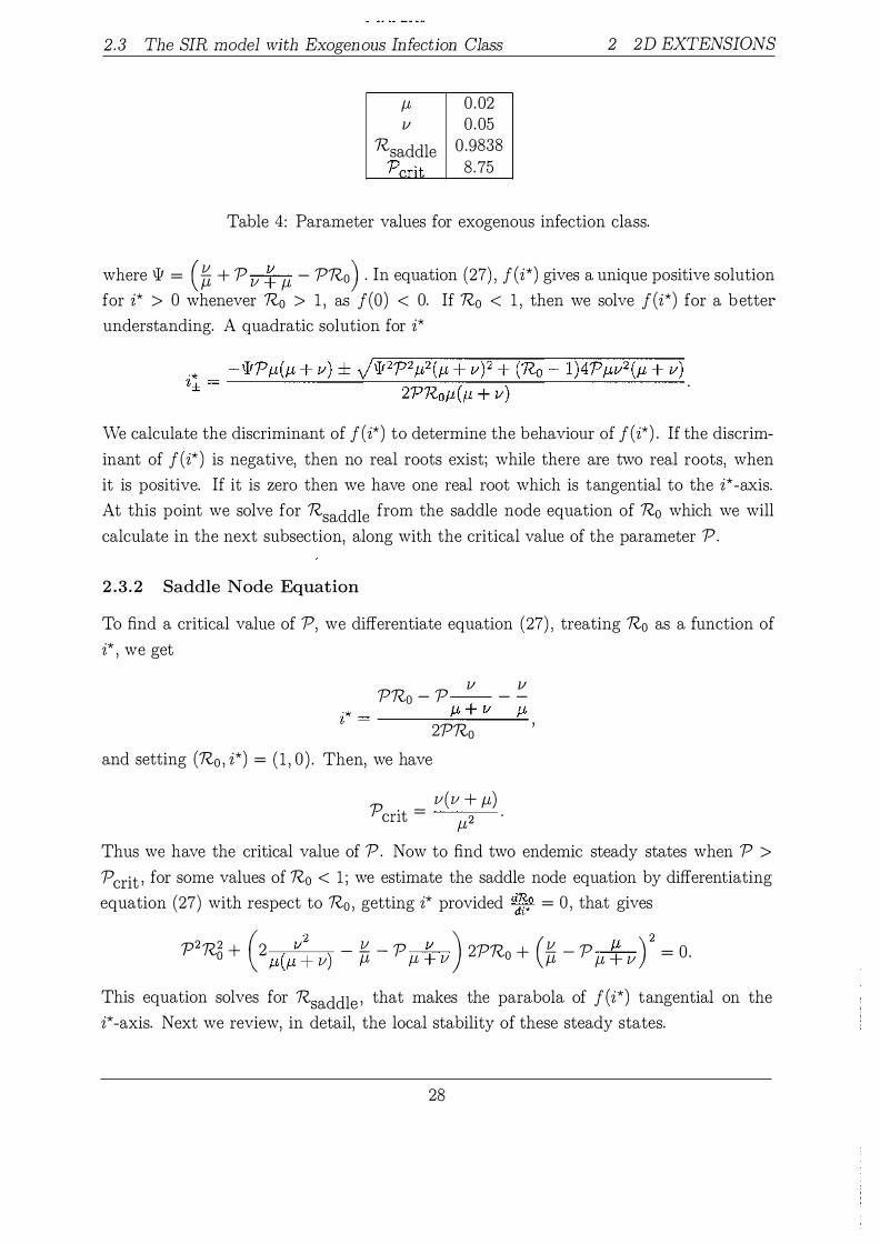
where \[! = (* + P v + f-l - PRo) . In equation (27) , f(i*) gives a unique positive solution for i* > 0 whenever R0 > 1 , as f(O) < 0. If R0 < 1 , then we solve f (i*) for a better understanding. A quadratic solution for i*
We calculate the discriminant of f (i*) to determine the behaviour of f (i*) . If the discriminant of f (i*) is negative, then no real roots exist; while there are two real roots, when it is positive. If it is zero then we have one real root which is tangential to the i*-axis. At this point we solve for Rsaddle from the saddle node equation of R0 which we will calculate in the next subsection, along with the critical value of the parameter P.
2.3.2 Saddle Node Equation
To find a critical value of P, we differentiate equation (27) , treating R0 as a function of i* , we get
l/ l/ PRo - P-- - -
i* = ___ ___!.J-L_+_v _ __!__f-l 2PR0
and setting (R0 , i*) = ( 1 , 0 ) . Then, we have
p . _ v(v + J-L) cnt - f-l2 ·
Thus we have the critical value of P. Now to find two endemic steady states when P >
Pcrit ' for some values of R0 < 1 ; we estimate the saddle node equation by differentiating equation (27) with respect to R0 , getting i* provided d�o = 0 , that gives
'P2R6 + ( 2 J-L(:: v) - * - P f-l -f- v) 2PR0 + (* - P f-l � v ) 2 = 0 .
This equation solves for Rsaddle ' that makes the parabola of f (i*) tangential on the i*-axis. Next we review, in detail, the local stability of these steady states.
28

2.3 The SIR model with Exogenous Infection Class 2 2D EXTENSIONS
2.3.3 Stability
In this subsection to investigate the stability of the infection-free and endemic steady states, we linearise equations in system (26) to find the Jacobian matrix ( -J-L - (Ji -(Js ) J =
-P(Ji - v P(J - P(Js - 2P(3i - (J-L + v) .
For the infection-free steady state (s , i) = (1 , 0) , the Jacobian matrix becomes ( -J-L -(3 ) ]infection-free = -v _ (J-L + v) ·
(28)
(29)
Now this matrix have T = -2J-L-V, and .6.. = ( 1-R0) (J-Lv+J-L2) respectively. If R0 < 1 , then trace is negative and the determinant is positive, meaning that the infection-free steady state is stable. If 7?0 > 1 , then the infection-free steady state is unstable as T, .6.. < 0 .
The Jacobian matrix for the endemic steady state, when P = 0 , is
v(J-L� v) ) . - (J-L + v) (30)
This matrix has T = -J-L(Ro + 1 ) - v and .6.. = (Ro - 1 ) (J-Lv + J-L2) respectively. If R0 > 1 , then T < 0 with .6.. > 0. Thus the endemic steady state is stable for R0 > 1 .
To study the endemic steady state for P =I= 0, we put the value for s* in the Jacobian matrix ( 28) in terms of i* ,
This has
( (3 '* � ) -f-L - 'Z+ - J.L+f3i'+. -P(Ji� - v P(J - (2P(3i� + J.L�/1+ + J-L + v)
.
.6.. = (2P(3i* J-L - 2P(32i*2 - P(32i* + v(Ji* + "V + u(Ji* + , ,2 ) - f3J-L(Pf3i� + v) . + + + + + r r + r f-L + fJi+
Evaluating the above Jacobian matrix by substituting the value for i� and using Table 4 for parameter values, we find that T+ < 0 and .6..+ > 0 for P > Pcrit and Rsaddle <
29

2.3 The SIR model with Exogenous Infection Class 2 2D EXTENSIONS
Exogenous Infection Model Bifurcation Diagram
A saddle
0.6 0.7 0.8 0.9 1.1 1.2 1.3 1.4 1.5
Figure 17: Bifurcation diagram for the SIR model with exogenous infection class. Labels are as in Fig. 5. The critical value of P for this class is v(vtf.L) . f.L
R0 < 1 . Hence, we have a stable endemic steady state i:+ . For R0 > 1 and all P, the endemic steady state is stable.
This has
and
]endemic-( -J-L - j3i� - f.L:fri:_
P/3 ) . -P{3i� - v P/3 - (2P{3i� + f.L�f3i:_ + J-L + v)
P{32i� - (2P + 1){32i� - 2P{3i�J-L - vj3i� - J-LV - 3J-Lf3i� - 2J-L2 T_ = ------�----�--------------------------------�
1-L + {3i":_
We find that for P > P crit and Rsaddle < R0 < 1 , an unstable endemic steady state i� is present as L , .0,._ < 0, while endemic steady state is stable for R0 > 1 and for any P.
Thus we have multiple endemic steady states for P > P crit and Rsaddle < Ro < 1 and only a stable endemic steady state for all P and R0 > 1 .
30
2.3 The SIR model with Exogenous Infection Class 2 2D EXTENSIONS
a) b)
o.l 0.1
Figure 18 : Phase-Planes for the SIR model with exogenous infection class for P = 0 < Pcrit when: (a) Ro = 0 .6 < Rsaddle ; (b) R0 = 2 within triangle s + i = 1 .
2 .3 .4 Bifurcation Analysis
The stability of the infection-free and endemic steady states for all values of R0 and P is the same as in Sect . 2 . 1 and Sect. 2 .2 . Figure 17 illustrates the asymptotic behaviour of these solutions to the system of equations (26) . Again, the dynamics are similar to those in Sect . 2 . 1 .
2 .3 . 5 Phase-Plane Analysis
Now, consider the triangular region X and plot phase-planes so that we can develop a better understanding of the above results. Again we categorise based on different values of R0 and P. Arrows show the flow of the solutions; dashed lines represent nullclines ; and black dots are steady states. This model gives similar results to those in Sect . 2 .
1 . p = 0 • Ro < 1
A stable infection-free steady state is present in Fig. 18 (a) . • Ro > 1
There is an unstable infection-free steady state and a stable endemic equilibrium in Fig. 18 (b) .
2 . 0 < P < P crit
31

2.3 The SIR model with Exogenous Infection Class
a ) b } �'"r:iJ·FtOm.ut{ee fMhJ·t:'US M.I*O<C1 fle¥0$ j's ?� e; SI (I • t·� l� +l"JJ)h"J• !JW'"'ro}i+r:q !l• J1 zu:�o.os ?:S
2 2D EXTENSIONS
s'•.W·FtOm.�sl(eJ"'�·;r.�r l'l);lii0.Q/ �:J- 1 2 !'" ?RSet.�llfl· t • � (m::i + rt.N't; ·{W,.I'lllt+w{l· U 001'0]5 P•S I
i I
i '
j I I l ' j
· · · j OJ 0.1
Figure 19 : Phase-Planes for exogenous infection class for P - 5 < Pcrit when: (a) Ro = 0 .6 < Rsaddle ; (b) Ro = 1 .2 .
a ) I S''"'n.l·�l'li:.!SI(mlirt./bJ·m.J$ i' 1 ?Ri mus:ltl· s· �tw• 11.-1:'1.1 ·iSJ +ru)l+rtJt1·l)
o.•
:;u•OM RG*'!l! rti*OG5 P•$JS.
IJ
b) s':C.�·Ort55sl•O:.D:2s p_.�.(;{1 •!·�1+0.0S.(I·S·f3·0-t2l
01
1 1
O,f
Figure 20: Phase-Planes for exogenous infection class for P - Pcrit = 8 .75 when: (a) R0 = 0 .6 < Rsaddle ; (b) R0 = 2 .
32

2.3 The SIR model with Exogenous Infection Class
!'111J.tl·�1CisH.G1t i'•D 1i${1+i}HMSH• Ht•G-Cll
2 2D EXTENSIONS
t''"'tx!•RlmJSI(!f!Jtrtt},'::·I!!IS i't?ROmi\H:·��� fnt.JQtllJ!I•iHm.i t()./}1 w·�ro;o>o� JhU I\Dt0.$3Je-
Figure 21 : Phase-Planes for exogenous infection class for P = 14 > Pcrit when: (a) 1?0 = 0.6 < Rsaddle ; (b) 1?0 = 0.9838 = Rsaddle ·
a ) b ) ftWJ·ROt::al�.lt�'ltu·mn nJ:J�Ol ftOl: l2 s'=M2·1l.o'!J« Jl·O,Oll
l1ll0,Hti(l·S•iji..;..O.C6{1�t·fi·002i !':;r;?RQ mui(t· t• i)t� +W.bJ· tm •rt�)f +ro(t •SJ W-"CCS P:;; H
I l :r
Figure 22: Phase-Planes for exogenous infection class for P Rsaddle < Ro = 0.99 < 1 ; (b) R0 = 1 .2 > 1 is of interest .
33
14 > Pcrit when: (a)
2.4 Summary 2 2D EXTENSIONS
• Ro < 1 A stable infection-free steady state in Fig. 19 (a) .
• Ro > 1 A stable endemic and an unstable infection-free steady states are present in Fig. 19 (b) .
3 . P = Pcrit
• Ro < 1 A stable infection-free steady state is present in Fig. 20 (a) .
• Ro > 1 There are two equilibriums: an unstable infection-free and a stable endemic steady states in Fig. 20 (b) .
4. P > Pcrit
• Ro < Rsaddle Only an infection-free equilibrium is present in Fig. 21 (a) .
• Ro = Rsaddle = 0 .9838 A stable infection-free steady state exists while there are two endemic steady states exist which coincide with each other in Fig. 21 (b) .
• Rsaddle < Ro < 1 There are stable and unstable endemic steady states and a stable infection-free equilibrium in Fig. 22 (a) .
• Ro > 1 An unstable infection-free and a stable endemic steady states are present in Fig. 22 (b) .
2 .4 Summary
We conclude that in two dimensional extensions of the SIR endemic model: R class susceptible in Sect. 2 . 1 ; nonlinear transmission class in Sect. 2 .2 ; and exogenous infection class in Sect . 2 .3 , for R0 > 1 , there is an unstable infection-free steady state and a unique stable endemic steady state, with a forward bifurcation at Ro = 1 when P < Pcrit · A backward bifurcation occurs at R0 = 1 when P > Pcrit · We have found some sub-critical endemic steady states when Rsaddle < R0 < 1 and P > P crit . Thus, these models exhibit the dynamics of backward bifurcation; multiple endemic steady states ; and the phenomenon of hysteresis for certain values of R0 less than one.
34

2.4 Summary 2 2D EXTENSIONS
In Sect . 2 .2, the SIR model with nonlinear transmission class have a function h(i) that may lead to the presence of a limit cycle about the steady state. From [6] , we have applied a theorem that fails to prove the existence of any limit cycles for the function h( i) = 1:�i. However, we have also applied Dulac's criterion which fails to exclude any limit cycles. This criterion can not tell us about the global stability of the non trivial steady state in this case. However, from the calculation of the stability of infection-free and endemic steady states, the bifurcation and the phase-plane analyses, we have found that this model also possess a backward bifurcation phenomena.
35

3 GENERAL ANALYSIS OF 2D MODELS
3 General Analysis of 2D Models In this chapter, we will examine several two dimensional extensions of the SIR endemic model: R class susceptible; nonlinear transmission class; and exogenous infection class, in a general manner and using a matrix framework. Consider the 0 DE system
dy dt = -My + f (y) . (31)
where M is a non-singular 2 x 2 matrix, y is the vector ( : ) and f (y) is a vector-valued
function. At the endemic steady state ¥- = 0 , -My + f (y) = 0 , where R0 is the same parameter used previously. Hence, we calculate Jvf and f (y) in such a manner that R0 = 1 defines a bifurcation point with either a forward or a backward bifurcation. Given these conditions, we have applied Taylor and binomial expansions to obtain results, using i* as
a small perturbation variable, about the infection-free steady state y = ( � ) .
The basic idea in this chapter is to apply a perturbation technique to compare the previous bifurcation analysis for endemic steady states ; and to establish that these perturbation results agree with the summary in Chapter 2. This will lay the framework for a general analysis model of these types.
3.1 Susceptible R Class
Consider the ODEs for a susceptible R class as given in Sect. 2 . 1 (see equations ( 1 2 ) ) . Taking basic reproduction number R0 = J-L � 1 and P is the ratio of transmission probabilities from the recovered and susceptible classes. Rescaling time so that J-L = 1 we rewrite equations (12) as ds
- 1 - R0Asi - s, dt di dt R0Asi + PR0A(1 - s - i)i - Ai,
where A = f-L�'Y (See Table 5) . Separating linear and quadratic terms, we have equation (31) where,
and
Jvf - ( 1 0 ) -0 A(1 - PRo) '
f ( ) = ( 1 - R0Asi ) . y R0A(si - P(s + i)i)
36

3. 1 Susceptible R Class 3 GENERAL ANALYSIS OF 2D MODELS
Notation Description A fL .:t.. 'Y
fL c 1!:_±._!!_
(p + vUp + 'Y) V f-LV 15 p + v [3 dfJ_
fL B !:!._±}_
fL
E (p + v) (p + "f) - K"(V fLY
F p +- (5 X ,\
Ti
Table 5 : Frequently Used Notation in Chapters 3 and 5
Setting time derivatives of this matrix system to zero we have
(32)
At a steady state when y• � ( ;: ) , equation (32) becomes
y* = M-1 f(y*) . (33)
Thus
* ( s* ) ( 1 - R0As*i* ) y = i*
= Ro(s*i* - Ps*i* - Pi*2) ( 1 - PR0)-1 . (34)
Applying a Taylor series expansion about i* = 0, to s* and R0 we gain quadratics expressions in i* and ignore cubic and higher order terms.
(35) s* 1 + i*s� + i*2s; + O(i*3 ) ,
i* + i*2 (R01 + sr) + O(i*3 ) .
37
3. 1 Susceptible R Class 3 GENERAL ANALYSIS OF 2D MODELS
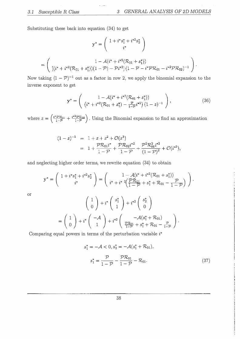
Substituting these back into equation (34) to get
y* = 1 2 ( 1 + i* s* + i*2 s* ) i*
Now taking (1 - P)-1 out as a factor in row 2 , we apply the binomial expansion to the inverse exponent to get
(36)
where z = ( i*J'_"i§1 + i*:r:._�02 ) • Using the Binomial expansion to find an approximation
and neglecting higher order terms, we rewrite equation (34) to obtain
or
y* = ( 1 + i*st + i*2s� ) = ( 12 -(PA��*1 + i*2 (Rm + st) )
p ) ) . i* i* + i* 1 '_'"' p + st + Ro1 - 1 _ p
( � ) + ;· en + i*' ( � )
= ( 1 ) + i* ( -A ) + i*2 ( PRo1-A�t + Rm)
P ) . 0 1 1-P + s1 + Rm - 1-P Comparing equal powers in terms of the perturbation variable i*
s� = -A < 0 , s; = -A(s� + 1?01 ) ,
* P PRm s1 = -- - -- - Rm. 1 - P 1 - P
38
(37)

3.2 Nonlinear Transmission Class 3 GENERAL ANALYSIS OF 2D MODELS
R dass l\Iodel s· = 1 + ts1 + i2"b"2, Ro = 1 + tRo1 + /Rm
* s
I I
I
I
� : � :
/ -
Rol < 0
s," < 0
Figure 23: Enlarged top-center part of Figure 5 . A clearer view for st < 0 , and the values for R01 as we perturb the variable i*. Unbroken lines show stable steady states while broken lines signify unstable. The curve R01 < 0 when P > P crit and curve R01 > 0 when P < Pcrit ·
At the critical value of P, R01 = 0 , st = -A then equation (37) becomes
and hence
Pcrit = 1 + � • If P > P crit , then Ro1 < 0 and a backward bifurcation occurs.
• If P < P crit , then Ro1 > 0 then a forward bifurcation occurs.
This is the same as in Sect . 2 . 1 , and is illustrated in Fig. 23. This sketch shows that using the Taylor series expansion, we have found results consistent with those in Sect. 2 . 1 .
3 . 2 N onlinear Transmission Class
In this section, we will investigate the nonlinear transmission model using a general framework. We review the system of ordinary differential equations (18) in Sect. 2 .2 . with nonlinear force of infection ' ,\ = /3i(1 + h( i) ) ' and h( i) = 1 r�i . For more details see Sect . 2 .2 and Games et al. [6] . R0 = (J-L!'Y) and P are as in Sect. 2 .2 . We rewrite the
39

3.2 Nonlinear 'I}ansmission Class 3 GENERAL ANALYSIS OF 2D MODELS
equations (18) as
ds dt - f.L - Ro (f.L + !') (1 + h(i) ) si - f.LS, di dt Ro (f.L + !') (1 + h(i) ) si - (f.L + !')i .
Rescaling time, so that f.L = 1 we have
ds dt di dt
( 1 + 2Pi) 1 - R0Asi 1 + Pi - s ,
R A . ( 1 + 2Pi) _ A . 0 S'l 1 + Pi z ,
where A = 1-l�'Y and 1 + h(i) = \�2�i · In matrix form, we consider equation (3 1 ) where
!VI = ( 1 0 ) = ( s ) ( ) = ( 1 - R0Asi ( 11��i) ) 0 A ' y
i ' f y R0Asi ( 11�2�i)
Setting '!f.' � 0, for a steady state y* � ( :: ) , equation (32) becomes
Hence
* = Jvf-1!( *) = ( 1 0 ) ( 1 - R0As*i* ( 11���* ) ) y y 0 A-1 /f) A * '* ( 1 + 2Pi* )
. '�O S 'l 1+Pi* ( 1 + Pi* - ARos*i* - 2P AR0s*i*2 ) * _ 1 + Pi* y - Ros*i* + 2PR0s*i*2 ·
1 + Pi* Using the binomial expansion (1 + Pi*)-1 = 1 - Pi* + P2i*2 + O(i*3) and ignoring higher order terms, we get
* = ( s* ) = ( 1 - AR0s*i* - PAR0s*i*2 ) . y i* Ros*i* + PR0s*i*2 (38)
We apply a Taylor series expansion, in equation (38) finding quadratic terms for s* and Ro, using a perturbation variable i* . From equation (35 ) , we have s*, R0 and R0s*i* so we expand R0s*i*2 = i* (i* + i*2 (st + R01 ) ) = i*2 + 0 (i*3 ) . Ignoring higher order terms,
40

3.2 Nonlinear Transmission Class 3 GENERAL ANALYSIS OF 2D MODELS
* s
I I
Non linear Transmission s"" = 1 + iS1 + P��, Ro= 1 + i*Rm + P\Wl
, ,
� ,
' •
• ,
Figure 24: Enlarged diagram taken from Fig. 1 1 . Labels are as in Fig. 23.
we substitute these values back into equation (38) getting
or
y* = ( 1 + i* st + i*2 s� ) = ( 1 - A( i* + i*2 ( st + R01 - P)) ) i* i* + i*2 (st + Ro1 + P) ' ( � ) + i* en +i'' ( � )
( � ) +i* ( -: ) +i*' ( -A�o::/!;P) ) .
Comparing terms with equal power of i* we get
s� = -A < 0 , s; = -A(Rol + s� - P) ,
s� = -P - R01 . (39)
At the critical value of P, R01 = 0 we have st = -A. Thus, equation (39) becomes P = -st = A.
Pcrit = 1 + � • If P > P crit , then R01 < 0 and a backward bifurcation occurs.
• If P < P crit , then Ro1 > 0 and a forward bifurcation occurs.
These results are consistent with those in Sect. 2.2 . Fig. (24) shows that a backward bifurcation occurs when R01 < 0 , while forward bifurcation occurs when R01 > 0 .
41

3.3 Exogenous Infection Class 3 GENERAL ANALYSIS OF 2D MODELS
3 . 3 Exogenous Infection Class
In this section, a system of differential equations for the SIR model with exogenous infection class is studied. We consider the ordinary differential equations from Sect . 2.3 .
ds dt - f-l - {Jsi - f-LS, di dt P{J(1 - s - i)i + v(1 - s) - (f-l + v)i.
(40)
We rescale time to have f-l = 1. The transmission rate fJ = Ro (f-l v+ v)f-L and the parameter
P are as in Sect. 2 .3 . Substituting fJ in equation ( 40) we get
ds dt di dt
1 - R015si - s , - c -
PR0'D(1 - s - i)i + -=-(1 - s) - Ci. 'D
See Table 5 for notations 15 and C. In order to obtain matrix form, we take equation (31 ) , where
Setting 'J; = 0, for a steady state y* = ( ;: ) , we have equation (33 ) .
( 1 - R015s*i* ) y* = NI-1 f(y*) = (R0s*i* (C - P15) - P15i*2) ·
(C - PRoD) ( 41)
We apply a Taylor series expansion for s* and R0 , using i* as a perturbation variable.Ignoring cubic and higher order terms and substituting the quadratic terms from equation ( 35) back into equation ( 41) to get
-(
y* = 1 2 ( 1 + i* s* + i*2 s* ) i*
1 - 15(i* + i*2 (st + R01 ) ) ) [(i* + i*2 (st + R01 ) ) (C - P15) - P15Roii*2] ·
( C - P'D - i*PDR01 - i*2P'DRo2 )
42

3.3 Exogenous Infection Class 3 GENERAL ANALYSIS OF 2D MODELS
Taking (C _1PV) as a factor from row 2 to have
where
At this point, we apply a binomial expansion to obtain an approximation
- - 2 - 2 2 (1 - z) -1 = 1 + PVROl i* + P'DRo2 i*2 + p 'D R01
2 i*2 + O(i*3 ) . C - PV C - PV ( C - PV)
( 42)
Again we ignore cubic and higher order terms and substitute this back in equation ( 42) to obtain
or
y* = 1 2 = ( 1 + i*s* + i*2s* ) i* ( 1 - 15(i* + i*2 (s� + Ro1 ) ) ·* + ·*2 ( * + n + P15 ( Ro1 - 1 ) ) z z s 1 ''--01 C _ P'D
( � ) + i' ( sn + i'' ( � ) ( � ) + i' ( -� ) + i'' ( sj +;;:�ip�7�; 1 ) )
Comparing terms s� = -15 < 0, s; = -15(s1 + R01 ) ,
P15ROl * P15 C - PV + s1 + Ro1 - C - PV = 0
) ·
At the critical value of P, R01 = 0 we have s� = -15 and equation (43) becomes
- � -C - f.L p = -1 --15 = ----'p,-v p . _ v(J.L + v)
cnt - J.L'2 43
( 43)

3.3 Exogenous Infection Class 3 GENERAL ANALYSIS OF 2D MODELS
Exogenous Infection Model s'· = 1 + is1 + i2*S2, Ro = 1 + tRo. + p*Rm
* � s I
Rol < 0 ; ;
- I
Rot > 0
• "
Figure 25: An enlarged top-center portion of the bifurcation fig. (17) . Labels are as in Fig. 23.
Thus, we conclude with the following results
• If P > Pcrit , then Ro1 < 0 and a backward bifurcation occurs.
• If P < P crit , then R01 > 0 and a forward bifurcation occurs.
These results are consistent with those in Sect . 2.3 . It is clear from Fig. 25 that R01 < 0
gives backward bifurcation, while R01 > 0 gives forward bifurcation.
44

4 3D EXTENSIONS
4 3D Extensions In this chapter, we will investigate four different three dimensional extensions of the SIR endemic model. The two dimensional SEI model was examined in Sect . 2 .3 . Now, we include a recovered R class to make it three dimensional SEIR model (see Sect. 4. 1 , Sect . 4.2 & Sect. 4.3) . We will discuss three different SEIR models. Firstly, we present the general SEIR model then, we investigate two other SEIR models that have partial and full recovery respectively. The model in Sect. 4.4 is another three dimensional model which introduces a Carrier class ( C) , and c( t) , a proportion of the population which are carriers.
4.1 SEIR model
This model is similar to that which we have discussed in Sect . 2 .3 as a two dimensional model. This becomes a three dimensional SEIR model when a recovered class is also included. The SEIR model postulates long-lasting immunity after infection as there is no transition from the recovered class to the susceptible class [ 1 1] . The system of four differential equations describing this model is
ds dt de dt di dt dr dt
p, - {3si - p,s, ( 44)
{3si - P{3ei - (p, + v)e,
P{3ei + ve - (p, + "!)i ,
"f'l - p,r,
with r (t) = 1 - s (t) - i(t) - e(t) to keep equations (44) as a reduced three dimensional system. The parameters p,, "! and v are as defined in Sect. 2 .3 . This model is three dimensional and if P = 0, it becomes the classical SEIR model [ 12] . The basic reproduction number Ro = (J-l+�(J-l+v) is independent of P.
Studying the globally stability of the system ( 44) in the region { (s (t) , e (t) , i (t) ) : 0 :::; s (t) , e (t) , i (t) :::; 1 , s + e + i :::; 1 } is highly nontrivial. Because, to prove the global stability of such a high dimensional system is not usually possible .
45

4. 1 SEIR model 4 3D EXTENSIONS
4 .1 . 1 Steady State Solutions
Applying a qualitative approach, we find that the system ( 44) possess two steady states i .e . infection-free and endemic equilibriums. The infection-free steady state is (s , e , i ) = ( 1 , 0 , 0) . On the other hand, we have endemic steady state: when P = 0; and when P =/= 0 .
D 'T1 - 0 th d · t d t t ( * * '*) _ ( 1 tL(Ro-1) tL(Ro-1) ) ror r - , e en em1c s ea y s a e s , e , z - Ro , Ro (tL+v) , !3 ·
For P =/= 0 , the endemic steady states are
and
e* PRo (f-l + r) (f-l + v)i* + v2 '
with i* solves for
( 45)
where p = ( (tL+�J1�+v) + �-��� - ::�) . We have a unique positive solution i* > 0 for R0 > 1 , as f (O) < 0. For R0 < 1 , we solve f (i*) to find a quadratic solution for i*
.* p(f-l + r) (f-l + v) ± V p2 (!-l + v)2 [2f-lr + (f-l + r) ] + 4Pf-tv2 (Ro - 1) z ± = - 2PRo (f-l + r) (f-l + v) ·
For R0 < 1 , we have three possibilities for the solutions of f ( i*) . If the discriminant of f( i*) is positive, then we have two real roots and if it is negative, then we have no real roots. If it is zero , then graphically, the parabola of f (i*) opens upward and is tangential to the i*-axis. The value of R0 causing it to be tangential to the parabola on the i*-axis is denoted as Rsaddle .
4 .1 .2 Saddle Node Equation
In this section, we will look for the conditions of the critical point for P where backward bifurcation occurs. We find the critical value for P, therefore we can calculate the saddle node equation for R0 when P > P crit where backward bifurcation occurs. Treating Ro as a function of i* and differentiating equation ( 45) to get
46

4. 1 SEIR model 4 3D EXTENSIONS
J-l 0.02 I 0 .06 lJ 0.05
Pcrit 8 .75 n,::J.rlolP. 0 .977
Table 6: Parameter values for the SEIR model.
Setting (R0 , i*) = ( 1 , 0) to obtain the critical value
P . _ v(J-L + v)
cnt - J-l2 ·
We calculate the saddle node solution by treating R0 as a function of i* in equation (45 ) , for P > Pcrit ; and then at the saddle we have �";:0 = 0, which defines the minimum value of R0 . Substituting the value of i* into equation ( 45) to get the saddle node equation
2 2 ( 2v2 Pv v) ( v Pv ) 2 P R + - -- - - 2PR0 + - - = 0 0 J-L(J-L + lJ) J-l + lJ J-l J-l (J-L + lJ) .
This equation solves for Rsaddle , at which two endemic steady states coincide with each other, at the turning point with i-component i� = i>:_ = i* .
4 .1 .3 Stability
Linearising the ODE system (44) , the Jacobian matrix is
J ( -J-L - (3i 0 -(3s )
(3i -P(3i - (J-L + v) (3s - P(3e . 0 P(3i + v P(3e - (J-L + 1)
For the infection-free equilibrium (s , e , i) = ( 1 , 0, 0) , the Jacobian matrix becomes
]infection-free
( -J-L 0 -(3 ) 0 - (J-L + lJ) (3 0 lJ - (J-L + I)
( 46)
(47)
The essential sub-matrix is the second 2 x 2 diagonal block. The stability conditions for r and 6. read
T = -(2!-l + I + v) ,
6. = (J-L + I) (J-L + v) ( 1 - R0) .
47

4. 1 SEIR model 4 3D EXTENSIONS
From this we always have T < 0 but if R0 < 1 , then 6. > 0 and if R0 > 1 then, 6. < 0 for all parameters. Hence, we have found that the infection-free steady state is stable when R0 < 1 , and unstable when R0 > 1 .
F th d · ' l 'b · ' f m - 0 th ( * * '* ) _ ( 1 p,(no-1) p,(no-1) ) or e en em1c eqm 1 num, 1 r - , en s , e , z - no , no (p,+v) , f3 ,
]endemic
This leads to the characteristic equation w3 + a1w2 + a2w + a3 = 0 , where
a1 = v + 1 + (2 + Ro)J-L,
a2 = J-LRo (2J-L + v + 1) , a3 = J-L(Ro - 1) [J-L2 + J-L(v + !) + vrl ·
From the Routh-Hurwitz theorem, if the conditions (c1 ) a1 > 0 , (c2) a3 > 0 and (c3) a1a2 - a3 > 0 are true, then all the roots of the characteristic equation have negative real part which means stable equilibrium. First two conditions are true for R0 > 1 as a1 and a3 are both positive quantities. The third condition
is greater than zero, for all parameter values in Table 6 , hence it is also true. Thus, we say that a stable endemic steady state is present for R0 > 1 , by the Routh-Hurwitz criteria.
Now to find the stability of the endemic steady state when P =/= 0, we substitute the value of s� and e� into the Jacobian matrix ( 46) (in terms of i�) to get
J ( -J-L - (3i� 0
f3i� s+ 0 P(3i� + v
(48)
Pf3(J.L+'Y)i* . . . A (3 Pf3(J.L+'Y)i* where, S+ = Pf3q. +/ - (J-L + /) , S+ = -p (3z� - (J-L + V) and S+ = J.L+%i+ - Pf3i+ +/ . Now we have the characteristic equation w3 + a1w2 + a2w + a3 = 0 , where,
a _ (3J-L + !)v + (P(3i� + v)2 + (3i� (2J-LP + (3Pi� + v)
1 - P(3i� '
48
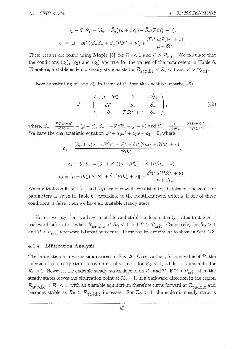
4. 1 SEIR model 4 3D EXTENSIONS
a2 = s+s+ - (S+ + S+) (M + (Ji�) - S+ (P(Ji� + v) ,
.* .. A '* (32i�M(P(3i� + v) a3 = (M + (Jz+ ) [S+S+ + S+ (P(Jz+ + v)] + (3 '* . M + z+
These results are found using Maple [5] ; for R0 < 1 and P > Pcrit · We calculate that the conditions (c1 ) , (c2 ) and (c3 ) are true for the values of the parameters in Table 6.
Therefore, a stable endemic steady state exists for Rsaddle < Ro < 1 and P > P crit .
Now substituting s=_ and e:_ , in terms of i=_ , into the Jacobian matrix (46)
J -{3j.l ) M+jW .. s_ , s_
p f3(J.l+'l )i':._ " '* A j3 p f3(J.l+'l )i':... where, s_ = Pf3i':... +v - (M + !) , s_ =-P(Jz_ - (M + v) and s_ =� - P/3i':...+v .
We have the characteristic equation w3 + a1w2 + a2w + a3 = 0 , where:
(3M + r)v + (P(Ji:_ + v)2 + (3i=_ (2MP + (3Pi=_ + v) al = ----------------�P-(J�i-�-----------------
a2 = S_S_ - (S_ + S_ ) (M + (3i=_ ) - S_ (P(3i=_ + v) , . . A (32i* M(P(Ji* + v) a3 = (M + (3i=_) [S_S_ + S_ (P(3i=_ + v)] + -
(3 .: . M + L
( 49)
We find that conditions (c1 ) and (c3) are true while condition (c2) is false for the values of parameters as given in Table 6 . According to the Routh-Hurwitz criteria, if one of these conditions is false, then we have an unstable steady state.
Hence, we say that we have unstable and stable endemic steady states that give a backward bifurcation when Rsaddle < R0 < 1 and P > Pcrit · Conversely, for R0 > 1
and P < Pcrit a forward bifurcation occurs. These results are similar to those in Sect . 2.3 .
4. 1.4 Bifurcation Analysis
The bifurcation analysis is summarised in Fig. 26. Observe that , for any value of P , the infection-free steady state is asymptotically stable for R0 < 1 , while it is unstable, for Ro > 1 . However, the endemic steady states depend on R0 and P. If P > Pcrit ' then the steady states leaves the bifurcation point at R0 = 1 , in a backward direction in the region Rsaddle < Ro < 1 , with an unstable equilibrium therefore turns forward at Rsaddle and becomes stable as Ro > Rsaddle increases. For R0 > 1 , the endemic steady state is
49

4. 1 SEIR model 4 3D EXTENSIONS
(s, i) = (1, 0) * s
0.8 ''·'··-·-·-·-·-·-·-·-·�·-·-·-·-·�·-·-·-·�-�����-0.6 -
P > Pcrit 0.4
0.2
*
i
Ruddle = 0.977 0.92 0.94 0.96 0.98 1.02 1 .04 1.06 1.08 1.1 1.12
Figure 26: Bifurcation Diagram for the SEIR model. Curves are s* and i* as the functions of R0. Continuous lines show stable steady state and broken lines are unstable steady states. There are curves for P < 'Pcrit ' P = 'Pcrit and P > 'Pcrit · For this model, p .
_ v(f.L+v)
cnt - f.L2 •
unique and stable for all 'P . This model also exhibits the phenomenon of hysteresis (see Sect . 2 . 1 ) .
4 . 1 . 5 Phase-Plane Analysis
In this section, we will analyse the phase-planes for the SEIR model, showing the trajectories of the three dimensional system onto two dimensions. The valid region in three dimensional space is a tetrahedron, for example s + e + i ::; 1 . We will look at a two dimensional projection of phase-space where the trajectories are confined to the triangle s + i ::; 1 . For a projection, trajectories of the solutions may appear to cross but they do not intersect in three dimensional space.
1 . p = 0
• R0 < 1 : A stable infection-free steady state is present in Fig. 27 (a) .
• R0 > 1 : There are one unstable infection-free steady state and a stable endemic equilibrium exist in Fig. 27 (b) .
� 2 . p = 2
• R0 < 1 : A stable infection-free steady state exists in Fig. 28 (a) .
50

4. 1 SEIR model
a s'=0..02·.\�ti•C.Ols l'r:l}.:P�'f+AROMSti·D.O"!l(>'.Pfm+-O.m}}Vt.PROHlal)
Figure 27: Phase-Planes for the SEIR Model for P Ro = 1 . 2 > 1 .
a :s':C . .Ol·A�si�Ml� I'•V\}?ft'it!i tA�O.OSJl·O-Oif{V�t.;.O.Qi)W.P.fWitO!J1)
4 3D EXTENSIONS
b t'=O.OZ·Aib);l•O.Cls i'��'(A.lPiU'tf tA�C.OStl·O�Jl(APROI tC.CT;�AP�I t0.01)
0 : when (a) R0 0.6 < 1 ; (b)
b t':0,02·A.FJlsi·O.olt !'•"': Pfti � f +Ait:O.OSti•O.Oi I{AP HO!+ GOm\APR:Ii Hl07;
Figure 28: Phase-Planes for the SEIR Model for P = 5 < Pcrit when: (a) R0 = 0.6 < 1 ; (b) Ro = l .2 > 1 .
5 1
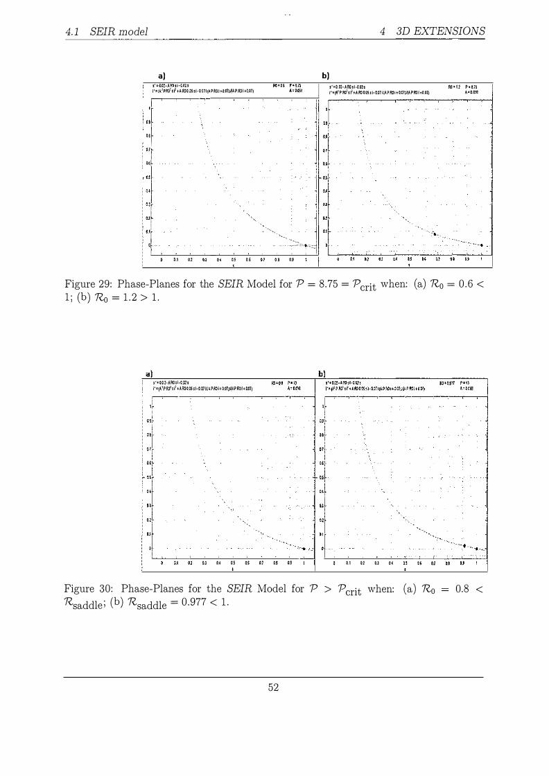
4. 1 SEIR model 4 3D EXTENSIONS
a) b) s : .... si� . s J':JA1PJ!i <r fA�O»>Ii· OQ!l(4PR?i+I.Oh;li.P�I tM)) s':0.02·Aithf·U2s ;·· WPRi .r, tRO o.11, H»n IAP"'l, o{J;>�;,PRO; .o_on RO* f1 P•.S,ii A.=ll�
,........., . -, 1 tr l t r 0!� �.J
l ��r i i . , J 01i 0 1 J I Of� ���
OJ I I I �J l Mf u
:1 ', ur I I '•. "f '• �
·<·--.... , 0.1 . of· · · �:�;'•;c�:1 or
0.1 Q2 u u M O! 01 O.S 03
Figure 29: Phase-Planes for the SEIR Model for P = 8.75 = Pcrit when: (a) R0 = 0 . 6 < 1 ; (b) R0 = 1 . 2 > 1 .
a s':002·AR0li·O,Ols ;· •(A'P Jii: f + AR!o.re •Ho !I(<?��+ oot))\APR?I +OMJ
N U U U U U U
b
0.1 02 OJ O.l
Figure 30: Phase-Planes for the SEIR Model for P > Pcrit when: (a) R0 Rsaddle ; (b) Rsaddle = 0 · 977 < 1 .
52
0.8 <

4. 1 SEIR model 4 3D EXTENSIONS
a) s'•OCl·ARO <I·Mls Rll•l.!!1 P•l5 l'•t/I'Pf<i sf tAROQ,0Ssi·O.I11{4PROit!I1)}\APRQI+M11 A•O.I!!
u u u u u " u u u
b) s'•M!·ARO<I·Uls i'•lA'Pf<isi'+AROO.IIsi•O.ili(IPROitailW,P�Ci+O�D
< . '
0 0.1 0.1 O.l
Rl• l.l P•IO A•OI!!
J [
.................. -···········--···· ................ ..!. __ ................................ - ............. .J
Figure 3 1 : Phase-Planes for the SEIR Model for P > Pcrit when: (a) Ro = 0 .987 < 1 ; (b) R0 = 1 . 2 > 1 .
• R0 > 1 : There are one stable endemic and unstable infection-free equilibriums are present in this Fig. 28 (b) .
3 . P = Pcrit
• R0 < 1 : A stable infection-free steady state exists in Fig. 29 (a) . • R0 > 1 : There are an unstable infection-free and a stable endemic steady
states in Fig. 29 (b) . 4. P > Pcrit
• Ro < Rsaddle : Only an infection-free equilibrium is present in Fig. 30 (a) . • Ro = Rsaddle = 0 .977: A stable infection-free steady state exists . At this
point , we have stable and unstable endemic steady states coinciding with each other in Fig. 30 (b) .
• Rsaddle < Ro < 1 : There are multiple endemic steady states: stable ; and unstable and a stable infection-free equilibrium in Fig. 3 1 (a) .
• Ro > 1 : A stable endemic steady state and an unstable infection-free steady state are present in Fig. 31 (b) .
53

4.2 The SEIR model with Partial Recovery 4 3D EXTENSIONS
4.2 The SEIR model with Partial Recovery
A special case of the SEIR model with partial recovery is the model by Van den Driessche et al. [14] . In this special case, the susceptible and recovered classes enter the exposed class at rates (3si and P(3si respectively. The system of four differential equations for this model is
ds dt de dt di dt dr dt
f-L - (3si - f-LS, (50)
(3si + P(3ri - (J-L + v)e + K/yi,
-P(3ri + ( 1 - "')'yi - J-Lr,
with r (t) = 1 - s (t) - i (t) - e (t) to keep equations (50) as a reduced three dimensional system. A rational number "' represents the unsuccessful recovery of the infectious class which re-approach the exposed class.
We find the basic reproduction number by solving equations in System (50) and considering the standard SEIR model when P = 0 . Obtain s* = f-1-�i* and e* = (
f-1-+:)i* by setting the right hand side of first three equations to zero, and substituting the values of s* and e* to get
.* f-L(f3v + "'IV - (J-L + 1) (J-L + v) ) z = ���--�������
j]( (J-L + I) (J-L + v) - "'lv) ·
Substituting the value of i (t) into s(t) to get s* = (f-!-+l)(f-1-;:)-K,Il/) . Now we know that R0 is the reciprocal of s* , then the basic reproduction number is Ro = ((f-1-+l) (::v)-K,v,) .
4.2.1 Steady State Solutions
By setting right hand side of system (50) to zero, we find the infection-free steady state is (s , e , i) =(1 , 0, 0) . The endemic steady state (s* , e* , i*) when P = 0, we have
( * * .*) = ( J-L (J-L + l)i* J-L(Ro - 1 ) ) s , e , z (3 .
, , (3 . J-L + z* v
If P =I 0 , then the endemic steady state for i* solves
J-LV2 (__!_ - 1) f( "* ) PR ( ) "*2 M .. "* no
0 z = o J-L + I + v z + z + ( ( ) ( ) ) = J-L + I J-L + V - K,VI
54
(5 1 )

4.2 The SEIR model with Partial Recovery
1-L I V K
Pcrit Rs:=trlrllA
4 3D EXTENSIONS
0 .02 0 .05 0 .05 0 .4 2 .6
0. 9545
Table 7: Parameter values for the SEIR model with partial recovery.
where M = (v(1 - PRo) + ( (�t:�)(�:0��vy) ) . The function f (i*) is a quadratic in i* and has a unique positive solution when R0 > 1 . For R0 < 1 , we may have a bit more complicated situation, depending on the values of the parameters (see Table 7) . The solution of the quadratic equation is
'* z± = 2PRo (f.L + v + r) '
-iii ± Vt
h C' �·1,· 2 4P�tv2 (�t+v+!)(l-Ro) F n 1 h h 1 · Th w ere 0 = m - ( (�t+'Y)(�t+v)-Kv'Y) . or '"O < , we may ave t ree so utwns. e solutions may be real or complex depending on nature of the discriminant £. If £ = 0 then, graphically the parabola of f( i*) is tangential to the i- axis. This happens when two endemic steady state coincides with each other whenever Ro = Rsaddle . This is a critical point at which the endemic steady states coincide. In next section, we will calculate the critical conditions for Pcrit and Rsaddle ·
4.2.2 Saddle Node Equation
Firstly, we find i* at the critical point , using the equation (51) and forming the implicit d . t' d'Ro 0 enva 1ve di* = . ( (PR 1 ) P�t(�t+v+'Y) ) '* Q - - ((�t+'Y) (�t+v)+KV/)
z = v�------��----�--�� 2PRo (ft + v + I) ·
We then calculate the critical value of Pcrit by setting (R0 , i* ) = (1 , 0) in i* to get
p . = [ (M + 1) (!-L + v) - lW!] cnt /V(1 - K) .
For P > Pcrit ' we get the saddle node equation by substituting i* into equation (51 ) ,
55

4.2 The SEIR model with Partial Recovery 4 3D EXTENSIONS
This equation solves for Rsaddle · In next section, we will consider the stability of the infection-free and endemic steady states, using the critical values of P and Rsaddle ·
4.2. 3 Stability
By linearising
J ( -M - f3i
f3i (1 0- P)
0
-Pf3i - (M + v) V
-f3s ) f3s + P/3(1 - s - e - 2i) + K:')' ,
- (M + !')
for the infection-free equilibrium (s , e, i) = ( 1 , 0 , 0 ) , becomes
(52)
(53)
We reduce this matrix to blocks, essential sub-matrix is the second 2 x 2 diagonal block. The trace and determinant of this sub-matrix are
The trace is always negative while � < 0 when 1?0 > 1 and � > 0 when 1?0 < 1 . For 1?0 < 1 , we have a asymptotically stable steady state. For 1?0 > 1 , the infection-free steady state is unstable.
Now, for the endemic steady state when P = 0 , the Jacobian matrix (52) will become
]endemic
This leads to the characteristic equation w3 + a1w2 + a2w + a3 = 0 where
a2 = M'Ro (2M + ')' + v) ,
a3 = M(Ro - 1 ) [M2 + MV + M/' - K:V')'] .
All the roots of this characteristic equation shows a stable steady state if the conditions ( c1 ) , ( c2) and ( c3) are true from the Rou th-H urwi tz criteria. It is easy to see that for
56
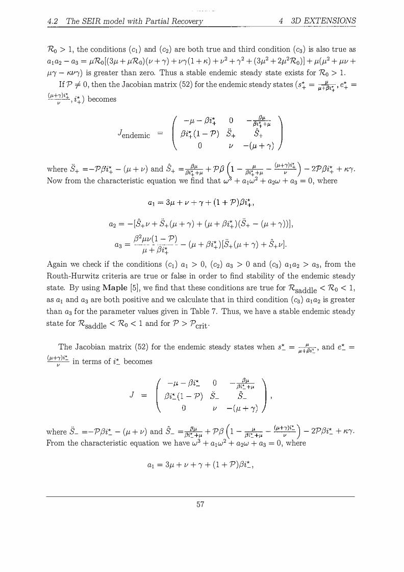
4.2 The SEIR model with Partial Recovery 4 3D EXTENSIONS
1?0 > 1 , the conditions (c1 ) and (c2) are both true and third condition (c3 ) is also true as a1a2 - a3 = J.L'i?o [(3J.L + J.LRo) (v + !) + v1(1 + K,) + v2 + 12 + (3J.L2 + 2j.L21?0) ] + J.L(J.L2 + J.LV + J.ll - K,l/1) is greater than zero. Thus a stable endemic steady state exists for R0 > 1 .
If 'P =1- 0 , then the Jacobian matrix (52) for the endemic steady states (s� = J.t�q_ , e� =
( + ) '* J.t "� t+ i* ) becomes lJ ' +
]endemic -
h S.. - --n/3 ·* ( ) d s� - {3j.t --n/3 r1 j.t (J.t+'Y)i+ ) 2--n/3 ·* w ere + --r 'Z+ - J.L + v an + - f3i+ +J.t + r \ - f3i+ +J.t - v - r z+ + /'\,/.
Now from the characteristic equation we find that w + a1w2 + a2w + a3 = 0 , where
a2 = - [s+v + s+ (J.L + 1) + (J.L + f3i� ) (s+ - (J.L + 1) ) ] ,
(32 J.LV(1 - P) .* . . �
a3 = (3 '* - (J.L + (3z+ ) [S+ (J.l + 1) + S+v] . J.l + z+ Again we check if the conditions (c1 ) a1 > 0 , (c2) a3 > 0 and (c3 ) a1a2 > a3 , from the Routh-Hurwitz criteria are true or false in order to find stability of the endemic steady state. By using Maple [5] , we find that these conditions are true for Rsaddle < Ro < 1 , as a1 and a3 are both positive and we calculate that in third condition (c3 ) a1a2 is greater than a3 for the parameter values given in Table 7. Thus, we have a stable endemic steady state for Rsaddle < R0 < 1 and for P > 'Pcrit ·
The Jacobian matrix (52) for the endemic steady states when s:_ = J.t�i:, , and e:_ = (J.t+'Y)i:_ in terms of i* becomes lJ -
J -
where S_ = -P(Ji:_ - (J.L + v) and §_ = f3if�j.t + P(3 ( 1 - f3it+J.t -(J.t+�)i:_ ) - 2P(3i:_ + /'\,/.
From the characteristic equation we have w3 + a1w2 + a2w + a3 = 0 , where
a1 = 3J.L + v + 1 + (1 + P)(Ji':_ ,
57

4.2 The SEIR model with Partial Recovery
8EIR with partial recovery (s, i) = '(1, o)
0.8
0.6 -
0.4 - p > pcrit
0.2
s '" 0
'Rsaddre= 0-.9545
4 3D EXTENSIONS
0.9 0.92 0.94 0.96 0.98 1.02 1.04 1 .06 1.08 1 .1
Figure 32: Bifurcation Diagram for the SEIR model with partial recovery. Labels are as in Figure 26. This model have P · = [(J.L+r) (J.L+v)-lwl)
. cnt 1v(l-��:)
a2 = - [S_v + EL (J-L + r) + (J-L + (3i*_ ) (S_ - (J-L + !) ) ] ,
a3 = f32J-Lv(1(3� P) - (J-L + (3i*_ ) [S_ (J-L + !) + S_v] . f-L + ?/ __
We use Maple [5] to calculate these conditions, for P > Pcrit and Rsaddle < Ro < 1 , the conditions ( c1 ) and ( c2) are true but condition ( c2) is untrue for parameters in Table 7,
thus this endemic steady state is unstable. When R0 > 1, and for all P, we estimate that the endemic steady state is stable, as all the conditions are true for certain parameters in Table 7.
In general, we understand that there are multiple endemic steady states for P > P crit and Rsaddle < Ro < 1 ; stable; and unstable. When R0 > 1 , we have stable endemic steady state for all P.
4.2.4 Bifurcation Analysis
Figure 32 illustrates that this phenomenon exhibits backward bifurcation, this is the same as in Sect. 4 . 1 .4.
58

4.2 The SEIR model with Partial Recovery 4 3D EXTENSIONS
Figure 33: Phase-Plane for the SEIR Model with partial recovery for P = 0 when: (a) R0 = 0 .7 < 1 ; (b) R0 = 1 . 2 > 1 .
4.2.5 Phase-Plane Analysis
We now study the phase-planes for the SEIR model with partial recovery class. In these phase-planes we derive three dimensional information from two dimensional projections (r (t) = 1 - s(t) - e(t) - i (t) ) . The solutions in these phase-planes may appear to cross each other only because of this projection. We use the numerical mathematical package MATLAB ODE45 [10] to understand these phase-planes. A number of shades and tints of grey colour are used for different solutions to represent different initial conditions.
1 . p = 0
• R0 < 1 : A stable infection-free steady state exists in Fig. 33 (a) .
• R0 > 1 : There are an unstable infection-free steady state and a stable endemic equilibriums in Fig. 33 (b) . p ' t 2 . P = �
• R0 < 1 : A stable infection-free steady state exists in Fig. 34 (a) .
• R0 > 1 : There are two stable endemic and an unstable infection-free equilibriums in Fig. 34 (b) .
3 . P = Pcrit
• R0 < 1 : A stable infection-free steady state is present in Fig. 35 (a) . 59
4.2 The SEIR model with Partial Recovery
a b
4 3D EXTENSIONS
Pfiauy[an;;·whm :Ro- >11'?#1'0/t .-�-�-·�r-·�,���-"'1·-� .
'Pn�;t-Figure 34: Phase-Plane for the SEIR Model with partial recovery for P = 1 . 3 = � when: (a) R0 = 0 .7 < 1 ; (b) R0 = 1 . 2 > 1 .
a) -������··��-"T"-��r-,-·-,...-......, 04� !
�35�
b)
0.15� 01� 005�
rl ��::§�::_�I or '--0,_2--'-0.3-0.4
Figure 35: Phase-Plane for the SEIR Model with partial recovery for P = 2 .6 = Pcrit when: (a) Ro = 0 .7 < 1 ; (b) R0 = 1 . 2 > 1 .
60

4.2 The SEIR model with Partial Recovery
a
4 3D EXTENSIONS
b
Figure 36: Phase-Plane for the SEIR Model with partial recovery for P > Pcrit when: (a) Ro = 0 .7 < Rsaddle ; (b) Rsaddle = 0.9545 < 1 .
a) b)
O>S ·
o�['-/� 02r 0.15 0.1 0.05 0.2 Figure 37: Phase-Plane for the SEIR Model with partial recovery for P > Pcrit when: (a) Rsaddle < Ro = 0.98 < 1 ; (b) R0 = 1 . 2 > 1 .
61

4.3 SEIR model with Full Recovery 4 3D EXTENSIONS
• R0 > 1 : There are an unstable infection-free and stable endemic steady states in Fig. 35 (b) .
4. p = 5 .2 > Pcrit
• Ro < Rsaddle : Only an infection-free equilibrium is present in Fig. 36 (a) .
• Ro = Rsaddle = 0.9545 : A stable infection-free steady state with stable and unstable both endemic steady states coinciding each other in Fig. 36 (b) .
• Rsaddle < Ro < 1 : There are stable and unstable endemic steady states and a stable infection-free equilibrium in Fig. 37 (a) .
• R0 > 1 : There is a stable endemic and unstable infection-free steady states in Fig. 37 (b) .
4.3 SEIR model with Full Recovery
This model is based on a paper by Van den Driessche [14] . The system of four differential equations for this model is
ds dt - t-t - {3si - f-LS, de dt di dt dr dt
{3si + P{3ri - (t-t + v)e ,
ve - (t-t + !)i ,
-P {3ri + 1i - t-tr.
(54)
with r (t) = 1 - s (t) - i (t) - e(t) to keep equations (54) as a reduced three dimensional system. In this special case, when entering the exposed class there is a successful recovery of infectious class. The basic reproduction number R0 is the same as in Sect . 4. 1 . As we have a successful recovery of infectious class thus K, = 0 .
4.3.1 Steady State Solutions
To find the steady state, we set the right hand side of equations (54) to zero. We calculate the infection-free steady state (s , e, i) = ( 1 , 0, 0) and the endemic steady state, when P = 0 . They are as in Sect. 4 .2 . I f P =I 0, then the endemic steady state for i* is the solution of
f-LV2 (_L - 1) PRoi*2 + Ni* + no = 0 . (t-t + !) (t-t + v) (t-t + v + 1)
62
(55)

4.3 SEIR model witb Full Recovery
fJ I 1/
Pcrit n�l'l rlrllP
4 3D EXTENSIONS
0.02 0 .05 0 .05 1 . 96
0 .9308
Table 8: Parameter values for the SEIR model with full recovery.
where N = ( v(�-;.:+�l) + (Jl+�ll�+v) ) . This equation has a unique positive solution for 'R0 > 1 . For 'Ro < 1 , we have more complicated situation which depends on the parameter values. The solution of this quadratic equation is
For 'Ro < 1 , we may have different solutions which may be real or complex. The nature of these solutions is determined by the sign of the discriminant of equation (55) . If the discriminant is negative, then we have no real roots; if it is positive, then we get two real roots; and if it is zero, then there is only one real root. In last case, the parabola is concave up and is tangential to the i- axis. In next section, we will calculate 'Rsaddle ' the minimum value of 'R0 ; and Pcrit ' the critical value for P.
4. 3.2 Saddle Node Equation
We find Pcrit from the equation (55) by differentiating 'R0 with respect to i* to get
Then we set ��0 I (l,O) = 0, in order to define the critical value of P
p . = (fJ + I) (fJ + v) cnt IV
·
Thus, we can find the saddle node equation for 'R0 when P > P crit . Hence, we put the value of i* back in equation (55) to get the saddle node equation for 'R0
63

4.3 SEIR model with Full Recovery 4 3D EXTENSIONS
This equation solves for Rsaddle · We will consider the stability of the steady states in next section using the critical values of P and Rsaddle ·
4.3.3 Stability
By linearising a system of equations (54)
J ( -fl, - f3i 0
f3i( 1 - P) -Pf3i - (J-L + v) 0 V
-f3s ) f3s + P/3(1 - s - e - i) - Pf3i ,
- (J-L + 'Y) (56)
for the infection-free equilibrium (s , e , i) = ( 1 , 0 , 0) , is the same as the Jacobian matrix ( 4 7) . The eigenvalues are same as for the matrix ( 4 7) . For R0 < 1 , we have an asymptotically stable infection-free steady state while for R0 > 1 , it is unstable.
For an endemic steady state (s* e* i*) = (__L J.L('R.o-l) J.L('R.o-l) ) when P = 0 we ' ' 'R.o ' 'R.o (J.L+v) ' (3 ' ' have the same Jacobian matrix (48) . This leads to the same characteristic equation w3 + a1w2 + a2w + a3 = 0 of the matrix (48) . Thus, a stable endemic steady state is present for R0 > 1 when P = 0 .
(J.L+!)i* Now, when P =f:. 0 , we put the endemic steady states for s� = � ' and e� = v + , in terms of i� , into the Jacobian matrix (56) to have
h S.. 'T)/3 ·* ( ) d s� 13J.L 'T)/3 (1 J.L (J.L+!)i+ ) 2'1")13 ·* F w ere + =- r z+ - f-L + v an + = f3i+ +J.L + r - f3i+ +J.L - v - r 'Z+ . rom the characteristic equation, we find that w3 + a1w2 + a2w + a3 = 0 , where
a2 = - [S\v + fh (J-L + 'Y) + (J-L + f3i� ) (S+ - (J-L + 'Y))] , /32 J-LV( 1 - P) '*
. . �
a3 = {3 '* - (J-L + f3z+) [S+ (f-L + 'Y) + S+v] . jJ, + 'Z+
We know that , from the Routh-Hurwitz criteria, all the roots of this characteristic equation are stable if the conditions (c1 ) , (c2) and (c3) are true. We calculate that these conditions are true for R0 > 1 as a1 and a3 both are positive quantities and a1 a2 - a3 is greater than zero using parameter values from the Table 8 . Hence, we have a stable
64
4.3 SEIR model with Full Recovery
endemic steady state when R0 > 1 , for all P.
4 3D EXTENSIONS
Now, for P > Pcrit and Rsaddle < R0 < 1 , we have calculated that these conditions are true, using Maple [5] . Thus we have a stable endemic steady state for P > Pcrit and Rsaddle < R0 < 1 . Now, we put the endemic steady states for s:_ = �' and
e:_ = (Jl.+�)i-:_ , in terms of i:_ into the Jacobian matrix (56) , thus we have ( - //. - (Ji* 0 -� ) f-V - {3t-:_ +Jl. 1 f3i:.. ( 1 - P) s_ s_
0 V -(f-t + !)
h S.. - P(J "* ( ) d SA - {3j.t P(J (1 J1. (Jl.+!)i-:_ ) 2P(3 "* Th" w ere, _ -- z_ - f-L + v an _ - f3i-:+Jl. + - f3i-:+Jl. -v - z_ . IS
leads to w3 + a1w2 + a2w + a3 = 0 , the characteristic equation, where,
a2 = - [S_v + B- (1-L + !) + (M + f3i*_ ) (S_ - (M + !)) ] ,
(32 f-LV(1 - P) . . A
a3 = (3 "* - (f-t + (Ji*_ ) [S_ (f-L + !) + S_v] . f-L + '/,_
When R0 > 1 , and for all P, we have a stable endemic steady state, as conditions (c1 ) , (c2 ) and (c3 ) are true for the parameters given in Table 8 . For P > Pcrit and Rsaddle < Ro < 1 , we calculate and use the values in Table 8 , that the condition (c2 ) is false while rest of the conditions are true by using Maple [5] . This implies that an unstable endemic steady state exists for P > P crit , Rsaddle < Ro < 1 .
Overall, we conclude that there are two endemic steady states present for P > P crit , and in the region of Rsaddle < R0 < 1 . These multiple endemic steady states give a backward bifurcation.
4.3.4 Bifurcation Analysis
Figure 38 summarises that a backward bifurcation occurs at R0 = 1 , this refers to sub-critical endemic steady states (shown as dashed and solid black lines) and a stable infection-free equilibrium. Thus, the dynamics of this system are similar to those of the SEIR class, described in Sect . 4 . 1 .
65
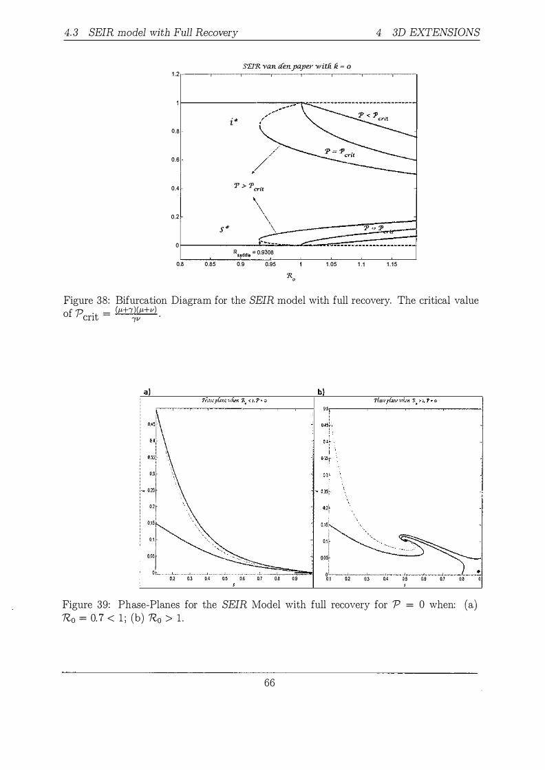
4. 3 SEIR model with Full Recovery 4 3D EXTENSIONS
S'EJ'R. van tfen yayeY witli fi = o 1 .2 ·---,.----·---.. -r---.... --r-.. ·-·-·--.. .,.._ .. ---.. --·r·-------r·---·---·-.. --·-,-----·-
i* 0.8
0.6
0.4 '1' > P crit
0.2
s *
0
Rsaddle = 0.9308
0.8 0.85 0.9 0.95 1 .05 1 .1 1 .15
'R 0
Figure 38: Bifurcation Diagram for the SEIR model with full recovery. The critical value of p . = (tL+!)(tL+v) cnt 1v ·
a
=I 02[ 0.151 i .:f or ....... ��"'"'�'�"""�--�"M,....;...,. .. ,"���-·���vJ...�--���, .. """""'�-�. -u u u u u u u u
b
l 0.15! oJ 005� 01 __ ,J.,...�-·�,.-J�"-"w� ... ��--,,:,��-�...,_"��"--"� ��� U U U M U U U M I
Figure 39: Phase-Planes for the SEIR Model with full recovery for P = 0 when: (a) R0 = 0. 7 < 1 ; (b) R0 > 1 .
66
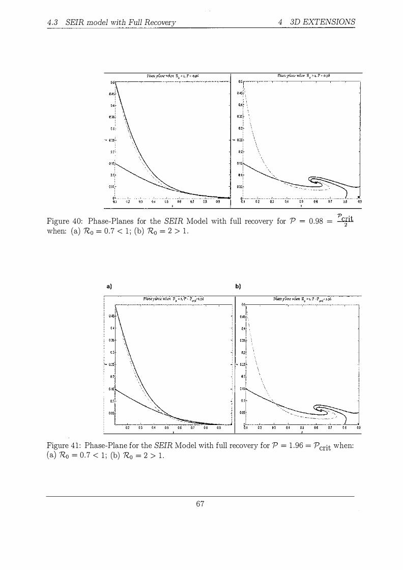
4.3 SEIR model with Full Recovery 4 3D EXTENSIONS
Figure 40: Phase-Planes for the SEIR Model with full recovery for P when: (a) R0 = 0 .7 < 1 ; (b) R0 = 2 > 1 .
a)
0.1$t 0,1 0.0$
--' ---' --.L'�--_�2�����--�---� 0.2 O.l M 0.5 0.6 O.i 0 a 0.9
b)
0.1 OQ5i· f �li_o.L,2 -o""-.3 -·
'P ,., .... ;l· f-0 .98 = �
Figure 41 : Phase-Plane for the SEIR Model with full recovery for P = 1 .96 = Pcrit when: (a) Ro = 0 .7 < 1 ; (b) R0 = 2 > 1 .
67
o.s

4.3 SEIR model with Full Recovery 4 3D EXTENSIONS
a)
0 51 0.451 Ol� o�l I o.�r 025� I nr I 0.15 I 0.1[ ' oo;l oLI ������������ 0.1 02 0.) 0.4 05
b)
U U U U U U U U I
Figure 42: Phase-Plane for the SEIR Model with full recovery for P > Pcrit when: (a) Ro = 0 .7 < Rsaddle ; (b) Rsaddle = 0 .9308 < 1 .
a b
Figure 43: Phase-Plane for the SEIR Model with full recovery for P > Pcrit when: (a) Rsaddle < Ro = 0.98 < 1 ; (b) R0 = 2 > 1 .
68
' I

4.4 The SIR Model with Carrier Class
4.3.5 Phase-Plane Analysis
4 3D EXTENSIONS
In this section, we will show the trajectories of the three dimensional system onto two dimensional in the following phase-planes for the SEIR model with full recovery. We use the parameter values from Table 8 and different shades and tints of colour grey show different initial conditions.
1 . p = 0
• R0 < 1 : Only a stable infection-free steady state is present in Fig. 39 (a) .
• R0 > 1 : There are one unstable infection-free steady state and stable endemic equilibrium exist in Fig. 39 (b) .
'T) = � 2 . r 2
• R0 < 1 : An stable infection-free steady state exists in Fig. 40 (a) .
• R0 > 1 : There are two stable endemic and unstable infection-free equilibriums in Fig. 40 (b) .
3 . P = 'Pcrit
• R0 < 1 : A stable infection-free steady state exists in Fig. 41 (a) .
• R0 > 1 : There are an unstable infection-free and a stable endemic steady states in Fig. 41 (b) .
4. p = 3 .92 > 'Pcrit
• Ro < Rsaddle : Only an infection-free equilibrium is present in Fig. 42 (a) .
• Ro = Rsaddle = 0.9308: A stable infection-free steady state and we have stable and unstable endemic steady states on top of each other in Fig. 42 (b) .
• Rsaddle < Ro < 1 : There are locally asymptotically stable and unstable endemic steady states and a stable infection-free equilibrium in Fig. 43 (a) .
• Ro > 1 : A stable endemic and an unstable infection-free steady states are present in Fig. 43 (b) .
4.4 The SIR Model with Carrier Class
There are some infectious diseases where a carrier may continue to infect others, but not suffer the symptoms of the infection itself. This introduces the Carrier class C. A proportion q( x) join the Carrier class on leaving the infective class when recovered. See,
69
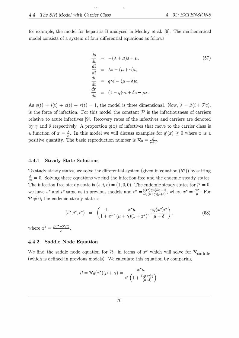
4.4 The SIR Model with Carrier Class 4 3D EXTENSIONS
for example, the model for hepatitis B analysed in Medley et al. [9] . The mathematical model consists of a system of four differential equations as follows
ds - (A + Jl)S + fl, (57) -dt di AS - (!l + l)i , - -dt de q1i - (!l + 5)c , -dt dr ( 1 - q)!i + be - Jlr. -dt
As s (t) + i (t) + c(t) + r(t) = 1 , the model is three dimensional. Now, A = j3(i + Pc) , is the force of infection. For this model the constant P is the infectiousness of carriers relative to acute infectives [9] . Recovery rates of the infectives and carriers are denoted by 1 and 6 respectively. A proportion q( x) of infectives that move to the carrier class is a function of x = � · In this model we will discuss examples for q' (x) � 0 where x is a positive quantity. The basic reproduction number is R0 = +!3 . J.L I
4.4.1 Steady State Solutions
To study steady states, we solve the differential system (given in equation (57) ) by setting �t = 0. Solving these equations we find the infection-free and the endemic steady states. The infection-free steady state is (s , i, c) = ( 1 , 0, 0) . The endemic steady states for P = 0 , we have s* and i* same as in previous models and c* =q(x*)!J.L(Ro -I) where x* = f3i* For no (J.L+i) (J.LH) ' J.L P =J. 0 , the endemic steady state is
(s* , i* , c*)
where x* = !3(i*+Pc*) . J.L
( 1 x* fl 1q(x*)i*) - 1 + x* ' (!l + 1) ( 1 + x*) ' fl + 6 '
4.4.2 Saddle Node Equation
(58)
We find the saddle node equation for R0 in terms of x* which will solve for Rsaddle (which is defined in previous models) . We calculate this equation by comparing
* x*f-L f3 = Ro ( x ) (Jl + I) = ( ) .
70
i* 1 + Pq(x*)! (J.LH)
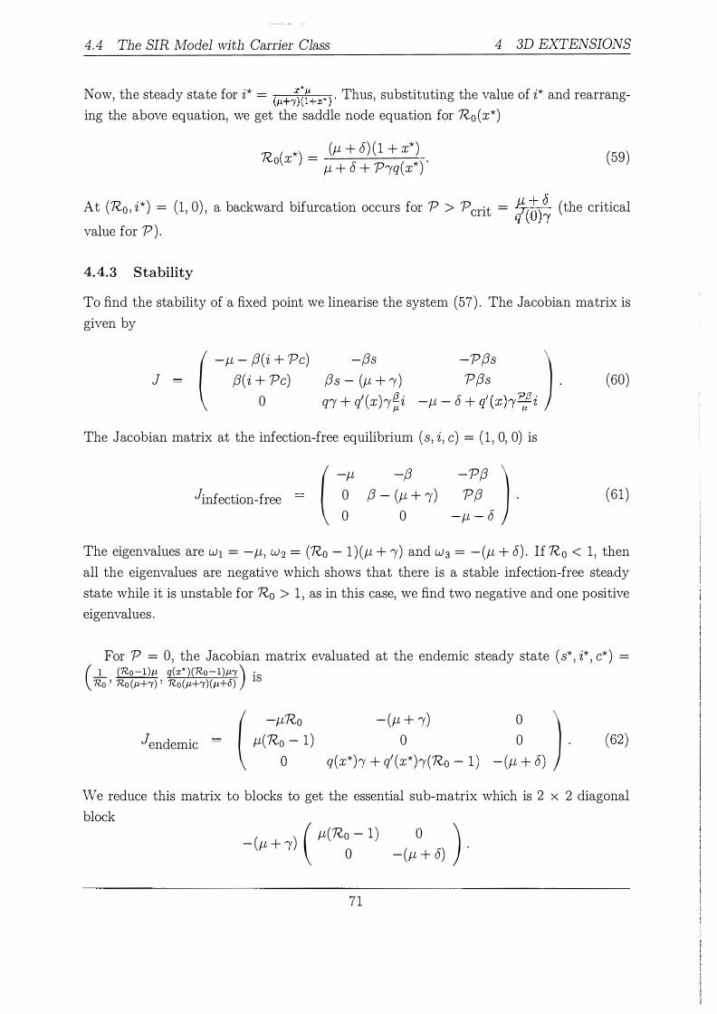
4.4 The SIR Model with Carrier Class 4 3D EXTENSIONS
Now, the steady state for i* = (i.L+,)�i+x* ) . Thus, substituting the value of i* and rearranging the above equation, we get the saddle node equation for R0(x*)
Ro(x*) = (p, + 6) (1 + x*) . p, + 6 + Prq(x*)
(59)
At (R0 , i*) = (1, 0) , a backward bifurcation occurs for P > Pcrit = �(1;)� (the critical value for P) .
4.4.3 Stability
To find the stability of a fixed point we linearise the system (57) . The Jacobian matrix is given by
J ( -p, - f3(i + Pc)
f3(i + Pc) 0
-f3s f3s - (p, + !) q[ + q' (x)r�i
-Pf3s ) Pf]s .
-p, - 6 + q' (x)rP:i
The Jacobian matrix at the infection-free equilibrium (s , i , c) = ( 1 , 0, 0) is
]infection-free
( -p, -/3 -P/3 ) 0 f3 - (p, + ! ) P f3 ·
0 0 -p, - 6
(60)
(61)
The eigenvalues are w1 = -p,, w 2 = (Ro - 1 ) (p, + r) and w 3 = -(p, + 6) . If R0 < 1 , then all the eigenvalues are negative which shows that there is a stable infection-free steady state while it is unstable for R0 > 1 , as in this case, we find two negative and one positive eigenval ues .
For P = 0, the Jacobian matrix evaluated at the endemic steady state (s* , i* , c*) = ( 1 (Ro -l)p, q(x* ) (Ro -l)�tl) · - lS Ro ' Ro (�t+i) ' Ro (�t+i) (p,+O)
]endemic
( -p,Ro p,(R�- 1)
-(p, + !) 0
q(x*)r + q' (x*)r(Ro - 1 )
0 ) 0 .
-(p, + 6) (62)
We reduce this matrix to blocks to get the essential sub-matrix which is 2 x 2 diagonal block
( ) ( p,(Ro - 1 ) 0 ) - p, + [ 0 -(p, + 6) .
71

4.4 The SIR Model with Carrier Class 4 3D EXTENSIONS
p, I 5
P crit for Example 1 Rsaddle for Example 1
Pcrit for Example 2
nSFl.rlrlle for Example 2
0 .02 0 .06 0 .025 0 .8333 0. 8299
0 .9 1 .09
Table 9 : Parameter values for the SIR model with carrier class.
This matrix has T = -(p, + l) [p,(Ro - 1) - (p, + 5)] and � = (p, + l) (p, + 5) (Ro - 1 ) . We have negative trace and positive determinant when 7?0 > 1 , this tells us that if R0 > 1 , then we have a stable endemic steady state whenever P = 0 .
When P f. 0, the Jacobian matrix (60) evaluated at the endemic steady state (equation (58) ) in terms of x*
]endemic -( -p,(1 + x*)
p,x* 0 ( *) q' (x* )!Rox* q X I + l+x*
_ PRo (J-L+'Y) ) l+x* PRo (J-L+!) l+x* s
(63)
where S = - ( u + 5) + q' (x* )IPRox* S = (J-L+!) (Ro-(l+x* )) . Again we find a characteristic ,-v l+x* ' l+x* equation w3 + a1w2 + a2w + a3 = 0, where
3p, + 4p,x* + (I + 5) (1 + x*) - q' (x*)rPR0x* - R0(r + p,) + p,x*2 (64) 1 + x*
a2 _ [(q(x*)rP - p,x*) (1 + x*) + q' (x*)rPRox*] Ro (M + 1) (S.. S) (1 *) _ SS ( 1 + x* )2 + p, + + x '
p,(p, + I) ( (p, + 5) (1 + x*) - q' (x*)rPRox* - Ro (M + 5i � ��x*)rPRo ) .
In the next few sections we will discuss different behaviours by numerically choosing two different examples for the function q(x* ) . We will check the conditions (c1 ) , (c2) and (c3 ) from the Routh-Hurwitz criteria in order to find the stability for different functions q(x* ) .
4.4.4 Examples 1 , 2
Here we use Maple [5] to evaluate steady states solutions, saddle node equations and stability. Example 1 when q' (O) > 0 ; and Example 2 when q' (O) = 0, both give backward
72
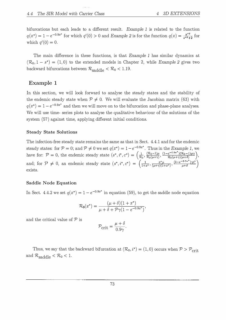
4.4 The SIR Model with Carrier Class 4 3D EXTENSIONS
bifurcations but each leads to a different result . Example 1 is related to the function
q (x*) = 1 - e-0·9x* for which q' (O) > 0 and Example 2 is for the function q(x) = x:;:2 for
which q' (O) = 0 .
The main difference in these functions, is that Example 1 has similar dynamics at
(1?0 , 1 - s*) = ( 1 , 0) to the extended models in Chapter 2 , while Example 2 gives two
backward bifurcations between Rsaddle < Ro < 1 . 19 .
Example 1
In this section, we will look forward to analyse the steady states and the stability of
the endemic steady state when P =I 0. We will evaluate the Jacobian matrix (63) with
q (x*) = 1 - e-0·9x* and then we will move on to the bifurcation and phase-plane analyses.
We will use time- series plots to analyse the qualitative behaviour of the solutions of the
system (57) against time, applying different initial conditions.
Steady State Solutions
The infection-free steady state remains the same as that in Sect . 4.4 . 1 and for the endemic
steady states: for P = 0 ; and P =I 0 we set q(x*) = 1 - e-o .gx* . Thus in the Example 1 , we
have for: P = 0 the endemic steady state (s* i* c*) = (_!_ (R.o-l)J.L (I-e-o .gx* ) (R.o -I)wr) ' ' ' R.o ' R.o (J.L+'Y) ' R.o (J.L+'Y) (J.L+O) ' d. f '1"> _j_ 0 d
. d ( * '* * ) - (-1- x* /), (1-e-0.9x* )'yi* ) an , or r 1 , an en em1c stea y state s , z , c - l+x* , (J.L+'Y) (l+x* ) , J.L+o
exists .
Saddle Node Equation
In Sect. 4 .4 .2 we set q(x*) = 1 - e-0·9x* in equation (59) , to get the saddle node equation
'T) ( *) = (p, + 6) (1 + x*) ''-'0 X 0 9 * ' p, + 6 + P1( 1 - e- · x )
and the critical value of P is p, + 6
Pcrit = 0 .91 ·
Thus, we say that the backward bifurcation at (1?0 , i*) = ( 1 , 0) occurs when P > Pcrit and Rsaddle < 1?0 < 1 .
73

4.4 The SIR Model with Carrier Class
Stability
4 3D EXTENSIONS
In this section, we will refer to the Jacobian matrix (63) in Sect . 4.4 .3 to study the stability
of the endemic steady states (s*, i* , c*) for P =/= 0. Equation (64) for q(x*) = 1 - e-0 ·9x* becomes
3j.L + 4J.Lx* + (r + 6) (1 + x*) - 0.9x*e-0·9x*!PR0x* - R0 (r + J.L) + J.LX*2 a - ----------�--�----�--------------------------------1 - 1 + x* '
[ ( ( 1 - c0·9x* )tPRo - f.Lx*Ro) ( 1 + x*) + 0.9x*e-0·9x*!PR6x*] (J.L + !) ( 1 + x*)2
+J.L(S + S) (1 + x*) - ss,
a3 = J.L(J.L + !) ((p, + 6) ( 1 + x*) - 0 .9,PRox*e-0 .9x* -Ro (P, + 6) -;�-
x=-0.9x* )tPRo )
'
where S = - ( 1 1 + 6) + (I-e-o·g'"*hPRox* S = (J.L+r) ('R.o-(l+x*)) . For this we choose different t"" l+x* ' l+x* values of x* , approximately between 0 .025 to 20, for the parameter values given in Table
9 . So we find that ( c1 ) , ( c2) and ( c3 ) are true for R0 > 1 whenever P 2: P crit for all
values of x*. Thus, there is a stable endemic steady state for R0 > 1 .
When Rsaddle < Ro < 1 and P > Pcrit ' we have conditions (c1 ) , (c3) are true but ( c2) is false as a3 < 0 for the values of x* between 0 .025 to 0 .8 ; while for other values, all
conditions (c1 ) , (c2) and (c3 ) are true. Therefore, we have multiple endemic steady states
in this region Rsaddle < R0 < 1 , that are stable and unstable, using the values in Table 9 .
Multiple endemic steady states leads to the phenomenon of backward bifurcation, which
occurs at R0 = 1 . Bifurcation Analysis
Fig. 44 shows a bifurcation diagram of Example 1 , for certain parameter values. We plot
three bifurcation curves against R0 using infection-free and endemic steady states. We
show that a forward bifurcation occurs for R0 > 1 if P ::; P crit , this shows the presence
of endemic infection for R0 > 1 . For Rsaddle < Ro < 1 and P > Pcrit = ���) , there are two sub-critical endemic
steady states present , one stable and the other unstable. From R0 = 1, an unstable
endemic steady state moves backward until it reaches Rsaddle ' at which point , it becomes
stable and moves forward. Thus a backward bifurcation occurs for at R0 = 1 .
74

4.4 The SIR Model with Carrier Class
. .... '
"'
0.9 0.8 -0.7 q(x) _ 1 _ e·o.gx 0.6 0.5 " 0.4 0.3 0.2 0.1
,.,.
4 3D EXTENSIONS
p > p crft
,.;·····"···
"·"··········
....
,,·' I' P = P crit !;'
I i i i i \ ! \ I \ i \ f \ � ' I
"...!
p < p crit
0 r-------------------------------�----�----------------------------
-0.1 0 0.2 0.4 0.6 1{sacfdfe - o.8299
0.8 1.2 1.4 1 .6 1.8
Figure 44: Bifurcation diagram for the SIR model with carrier class (Example 1 ) for the function q(x*) = 1 - e-O.Qx* . We show 1 - s* as a function of R0. Backward bifurcation occurs when P > Pcrit = ����) at (Ro , 1 - s*) = ( 1 , 0) .
Phase-Plane Analysis
We now analyse the phase-planes for the carrier class Example 1 in a (s* , i*) plane. The
dynamics of these phase-planes, using ODE45 (a numerical integration in MATLAB [10]) with different initial conditions (shown by different colours) is consistent with other models
as in Chapters 2 and 4 (which are plotted using PPLANE6 application in MATLAB [ 10] as they are in three dimensions and also have a special function q( x) that varies as x
varies) .
1 . p = 0
• R0 < 1 : A stable infection-free steady state is present in Fig. 45 (a) .
• R0 > 1 : There are an unstable infection-free steady state and a stable endemic
steady state in Fig. 45 (b) .
2. P = Pcrit
• R0 < 1 : Only a stable infection-free steady state is present in Fig. 46 (a) .
• R0 > 1 : In Fig. 46 (b) , there are unstable infection-free and stable endemic
steady states.
75

4.4 The SIR Model with Carrier Class
a )
o z,. ....... -........ , ...................... , ............................................. .,. .................... , .................... .,. .... -···········1 O.i&l· ��-l CJJ 0.12l
- 01� oosl �CJ O·:l<t ow� &�---Q'-, -o'_s-- (;$-�7··--ta-....__· o.!
J
b)
4 3D EXTENSIONS
1 ., I t ! L�.�H..J..voo-w . ..........J.�--w�-�-l�-·�·�-· -....::.••-·�--!� •• J o.& o.&S 0.1 o1> o.e o.es o� o>S 1 '
Figure 45: Phase-Plane for the Example 1 for P = 0 < Pcrit when: (a) R0 = 0 .7 ; (b) Ro = 1 . 1 .
3 . P > Pcrit
• R0 < 1 : We find only a stable infection-free equilibrium in Fig. 47 (a) .
• Ro = Rsaddle = 0.8299: A stable infection-free steady state exists and en
demic steady states coincide with each other as shown in Fig. 4 7 (b) . We see
that all the solutions goes to stable infection-free steady state.
• Rsaddle < Ro = 0.95 < 1 : In Fig. 48, there are stable and unstable endemic
steady states and an unstable infection-free equilibrium.
• Ro > 1 : There is a stable endemic and unstable infection-free steady states
are present in Fig. 48.
Time-series plot
In this section, we present a brief time-series analysis for the solutions of the ordinary dif
ferential equations (57) . The proportions of susceptibles (s (t) ) , infectives (i(t) ) , removed
(r(t ) ) and carrier (c(t) ) classes, in a constant population, move as time (in years) changes
and for different values of P and R0 . We use the initial conditions of (s* , i* , c* , r*) = (0 .5 , 0 .3 , 0 .2 , 0.0) in these plots. We also look for the transient part , which depends on
the initial condition, and the general part , which gives the steady state. The general part
is usually consistent in all time-series plots.
1 . p = 0
76

4.4 The SIR Model with Carrier Class
a ) 'ff:au ;'lime wfwn :Re �· (J:i < 1, T � (J.8J..U
02,--.----.
4 3D EXTENSIONS
b)
Figure 46: Phase-Plane for the Example 1 for P = 0 .8333 = Pcrit when: (a) R0 = 0 .7; (b) Ro = 1 . 1 .
a) b) Pfitlfe ;JfiJ.ne wlien 1{.t�"' :.tta z, o.S:9_9 < 1, P-" 1.666
Figure 47: Phase-Plane for the Example 1 for P = 1 .6 > Pcrit when: (a) R0 = 0 .7 < 1 ; (b) Ro = Rsaddle = 0 .8299 < 1 .
77
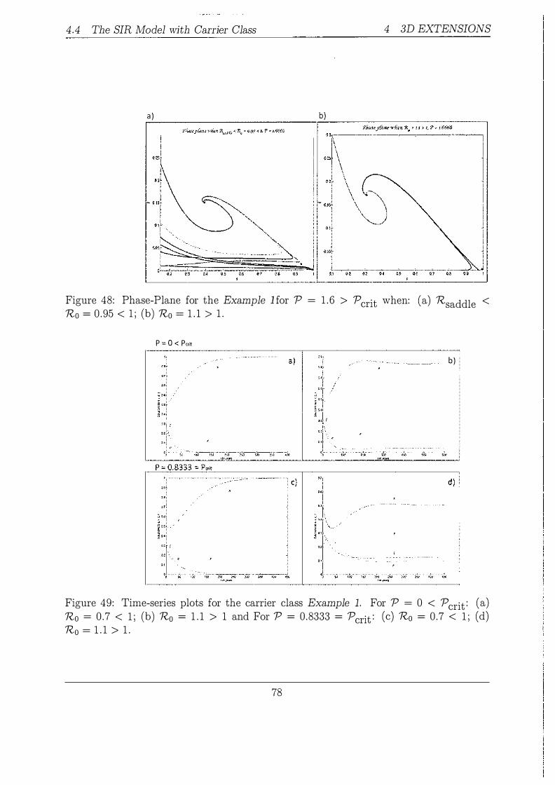
4.4 The SIR Model with Carrier Class
a )
4 3D EXTENSIONS
b)
Figure 48: Phase-Plane for the Example l for P = 1 . 6 > Pcrit when: (a) Rsaddle < Ro = 0 .95 < 1 ; (b) Ro = 1 . 1 > 1 .
P = 0 < P"it
b )
d )
Figure 49: Time-series plots for the carrier class Example 1 . For P = 0 < Pcrit : (a) Ro = 0 .7 < 1 ; (b) Ro = 1 . 1 > 1 and For P = 0 .8333 = Pcrif (c) Ro = 0 .7 < 1 ; (d) Ro = l . 1 > 1 .
78

4.4 The SIR Model with Carrier Class
P = 1.6 > Pcrit
4 3D EXTENSIONS
Figure 50: Time-series for q(x) = 1 - e-0·9x the carrier class Example 1 . For P = 1 . 6 > Pcrit = (a) Ro = 0 . 6 < 1 ; (b) Rsaddle = Ro = 0.8299 < 1 ; (c) Rsaddle < Ro = 0 .95 < 1 ; (d) R0 = 1 . 1 > 1 .
• R0 < 1 : In Fig. 49 (a) , a stable infection-free steady state is present as i ( t) decreases to zero and the proportion s(t) increases and give steady state .
• R0 > 1 : An unstable infection-free steady state and a stable endemic equilib
rium exist as i(t) decreases and give steady state. The proportion s(t) decreases
and increases rapidly and decreases slowly, then give steady state in Fig. 49 (b) .
2 . P = Pcrit
• R0 = 0 .5 < 1 : Fig. 49 (c) shows that the proportions i (t) , r (t) and c(t) decreases to zero and s(t) increases to 1 which gives a stable infection-free
steady state.
• R0 > 1 : In Fig. 49 (d) , we observe that the proportions go to steady states.
Thus, there are two steady states: an unstable infection-free; and a stable
endemic.
3 . P > Pcrit
• R0 < 1 : The proportion i (t) decreases to zero. Thus only an infection-free
equilibrium is present in Fig. 50 (a) .
79

4 .4 The SIR Model with Carrier Class 4 3D EXTENSIONS
• R0 = Rsaddle = 0 .8299: In Fig. 50 (b) , the proportions give steady states for
a longer period of time. Only a stable infection-free steady state exists. At this
point , we find stable and unstable endemic steady states intersect with each
other.
• Rsaddle < Ro < 1 : In Fig. 50 (c) , we find all proportions giving steady states
in shorter period of time. Thus, there are locally asymptotically stable endemic
steady state and a unstable infection-free equilibrium.
• R0 > 1 : There is a stable endemic and unstable infection-free steady states
are present as i (t) increases slowly and decreases quickly. On the other hand,
s ( t) decreases fast and then increases until steady state occurs in Fig. 50 (d) .
Example 2
In this section, first we will study the steady states, stability of the endemic steady state
when P =f. 0 for q' (O) = 0, a Example 2. Later, we will analyse bifurcation, phase-planes
and time-series plots.
Steady States Solution
The infection-free steady state remains unchanged, see Sect . 4.4 . 1 . For the endemic
steady state, we set q(x*) = x';2*:2 for all P. Thus in the Example 2, we have for: P = 0,
th d · t d t t ( * ·* *) _ ( 1 (Ro-1)J.L x*2 (Ro-1)f.L'Y ) d· f 'D -.L O e en em1c s ea y s a e s , z , c - Ro , Ro (J.L+i) , (x*2+2)Ro (J.L+i) (J.L+o) , an , or r r ,
d . t d t t ( * "* * ) - ( 1 x* J.L x*21i* ) an en em1c s ea y s a e s , z , c - Hx* , (J.L+i) (l+x* ) , (x*2+2)J.L+o ·
Saddle Node Equation
The saddle node equation (59) for q(x*) = x;2*:2 is
Ro (x*) = (p, + 5) ( 1 + x*) (x*2 + 2) (x*2 + 2) (p, + 6) + 1Px*2
.
This equation solves for Rsaddle ' but in this example we find two solutions for Rsaddle >
1 . The critical value for P is calculated numerically from q' (O) = 0 . Thus, using MAT
LAB [10] , we have Pcrit = 0 .9 .
Stability
We review the Jacobian matrix (63) to study the stability of endemic steady states
(s*, i* , c*) for P =I- 0 using Maple [5] . At this point we substitute q(x*) = x';2*:2 in
80

4.4 The SIR Model with Carrier Class
equations ( 64) to get
4 3D EXTENSIONS
* (41PRox*2 + Ro (J.-L + l) (x*2 + 2)2 ) a1 = J.-L(l + x ) + (J.-L + J) + (J.-L + I) - (l + x*) (x*2 + 2)2 '
= x*2Ro(J.-L + 1) [ (x* + 2) ( 1 + x*) (!P - J.-Lx*) + 41PRo] (S S) ( l *) _ SS a2 ( 1 + x*) ( x* + 2 ) 2
+ f.-L + + x '
J.-L(J.-L + 1) [ (J.-L + J) (x* + 2)2 ( ( 1 + x*) 2 - R0) - 1PRox*2 (5 + 4x*)] a3 = (1 + x*) (x* + 2)2 '
where S = - ( u + J) + 4'�PRox*2 S = (J.L+'l) (Ro-(l+x*)) We have observed that for all r (l+x*) (x*+2)2 ' l+x* ·
P there is a stable endemic steady state for R0 > 1 . When Rsaddle < Ro < 1 . 19 and P > Pcrit ' we have a untrue condition (c2) as a3 < 0 for some values of x* approximately between 0 .5 to 1 .2 ; while for the other values of x* , all conditions are true.
To calculate these results we use Maple [5] with the parameter values given in Table 9 . Thus, we find that there are multiple endemic steady states depending on the different values of x* in this region. For R0 > 1 , we have stable endemic steady state if P > Pcrit ' we have sub-critical endemic steady states for Rsaddle < 1?0 < 1 . 19 . This means the Example 2 exhibits different dynamics as there are two backward bifurcations.
This example is discussed in detail in Medley et al. [9] and have a different function q(>..) with a constant j , 0 :::; f :::; 1 , in terms of >.. , which has unit time-1 . However, this function exhibits similar dynamics to our chosen function q(x*) = x:;:2 .
Bifurcation Analysis
In Fig. 5 1 the bifurcation diagram for example q' (O) = 0 is presented. When P < Pcrit and Ro > 1 , we find a forward bifurcation. At Pcrit ' there is an inflection in the bifurcation curve, and this separates two qualitatively different behaviours. If P > Pcrit ' then we have multiple endemic steady states for some value of R0 • At R0 > 1 the curve leaves the trivial solution in a forward direction, then at 1?0 = 1 . 19 , the curve moves backward and the steady state becomes unstable. Until Rsaddle = 1 . 09 , the curve moves in a forward direction again, and the endemic steady state becomes stable.
Clearly, as q' (O) = 0, there can be no backward bifurcation at R0 = 1 , thus R0 = 1 is not a bifurcation point , in this example. We observe that , instead at R0 = 1 . 19 , there is a backward bifurcation for P > Pcrit ' where Pcrit is found numerically. Several multiple endemic steady states are present for Rsaddle < R0 < 1 . 19 . Thus in this model an
81
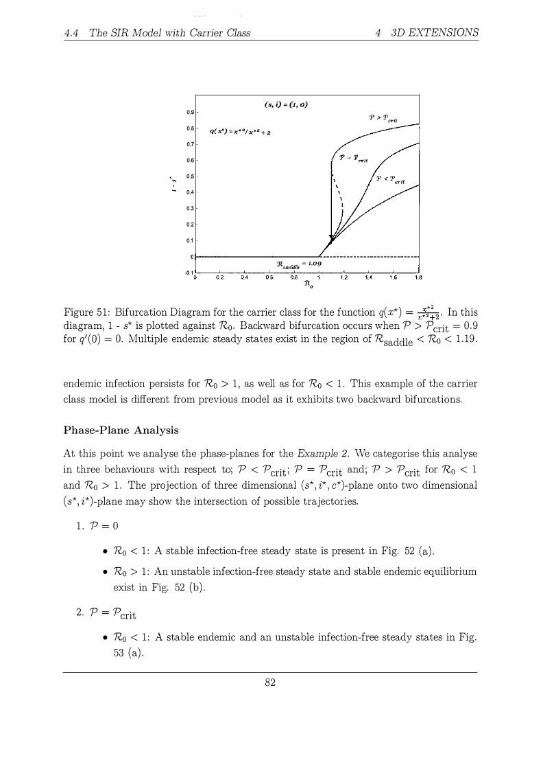
4.4 The SIR Model with Carrier Class
0.9 (s, i) = (1, o)
0.8 q( x*) = x•�; x•� + 2
. ...,
0.7
0.6 -
0.5
� 0.4
0.3 -
0.2 .
0.1
0 �------------------� 'Rsaaure = 1•09
4 3D EXTENSIONS
'1' > 1' . CTJt
'0·1 ol...--o-'-. 2--0-'-.4---'-o. s----'o.-s ---'----1-'-.2--1-'-.4---'-1.6----'1 .8
Figure 51 : Bifurcation Diagram for the carrier class for the function q( x*) = x;2*:2 . In this
diagram, 1 - s* is plotted against R0 . Backward bifurcation occurs when P > Pcrit = 0 .9 for q' (O) = 0 . Multiple endemic steady states exist in the region of Rsaddle < Ro < 1 . 19 .
endemic infection persists for R0 > 1 , as well as for R0 < 1 . This example of the carrier class model is different from previous model as it exhibits two backward bifurcations.
Phase-Plane Analysis
At this point we analyse the phase-planes for the Example 2. We categorise this analyse in three behaviours with respect to; P < P crit ; P = P crit and; P > P crit for Ro < 1
and R0 > 1 . The projection of three dimensional (s* , i* , c*)-plane onto two dimensional (s*, i*)-plane may show the intersection of possible trajectories.
1 . p = 0
• R0 < 1 : A stable infection-free steady state is present in Fig. 52 (a) .
• R0 > 1 : An unstable infection-free steady state and stable endemic equilibrium exist in Fig. 52 (b) .
2· P = Pcrit
• R0 < 1 : A stable endemic and an unstable infection-free steady states in Fig. 53 (a) .
82
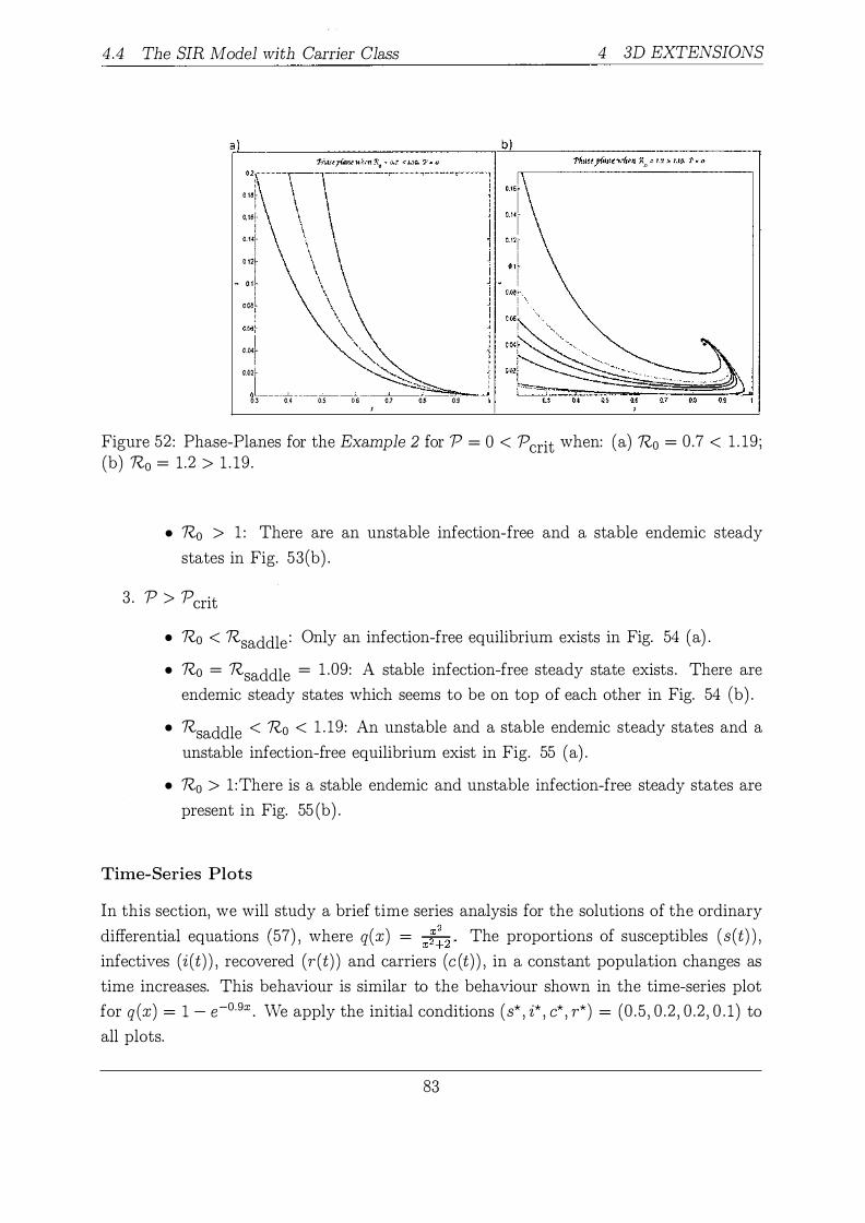
4.4 The SIR Model with Carrier Class
i O Hil-0 15'·
I C.H!·
_ j I ooal
I OO'T c.04r O.Oll l)L. ___ ---L,. __ . ----1..-------�--�J.-�� 0 oz 0.1 o.s 06 0.7 0$ os
J
4 3D EXTENSIONS
Figure 52: Phase-Planes for the Example 2 for P = 0 < Pcrit when: (a) Ro = 0.7 < 1 . 19 ; (b) R0 = 1 .2 > 1 . 19 .
• R0 > 1 : There are an unstable infection-free and a stable endemic steady states in Fig. 53(b) .
3 . P > Pcrit
• Ro < Rsaddle : Only an infection-free equilibrium exists in Fig. 54 (a) . • Ro = Rsaddle = 1 .09: A stable infection-free steady state exists. There are
endemic steady states which seems to be on top of each other in Fig. 54 (b) . • Rsaddle < Ro < 1 . 19: An unstable and a stable endemic steady states and a
unstable infection-free equilibrium exist in Fig. 55 (a) . • R0 > l :There is a stable endemic and unstable infection-free steady states are
present in Fig. 55 (b) .
Time-Series Plots
In this section, we will study a brief time series analysis for the solutions of the ordinary differential equations (57) , where q(x) = x�:2 . The proportions of susceptibles (s (t) ) , infectives ( i ( t) ) , recovered ( r ( t) ) and carriers ( c ( t) ) , in a constant population changes as time increases. This behaviour is similar to the behaviour shown in the time-series plot for q (x) = 1 - e-0·9x . We apply the initial conditions (s* , i* , c* , r*) = (0 .5 , 0 .2 , 0 .2 , 0 . 1) to all plots.
83
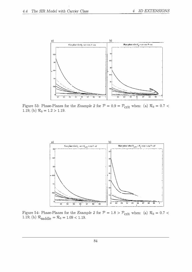
4.4 The SIR Model with Carrier Class
a )
4 3D EXTENSIONS
b)
Figure 53: Phase-Planes for the Example 2 for P = 0 .9 = Pcrit when: (a) R0 = 0 . 7 < 1 . 19 ; (b) R0 = 1 . 2 > 1 . 19 .
Figure 54 : Phase-Planes for the Example 2 for P = 1 .8 > Pcrit when: (a) R0 = 0 . 7 < 1 . 19 ; (b) 'Rsaddle = R0 = 1 . 09 < 1 . 19 .
84

4.4 The SIR Model with Carrier Class
a b
4 3D EXTENSIONS
11Um yt(nte. wJien :R'I) .., 1.3 .> I.Jg, 1'"' 1.8
Figure 55: Phase-Planes for the Example 2 for P = 1 . 8 > Pcrit when: (a)Rsaddle < R0 = 1 . 17 < 1 . 19 ; (b) R0 = 1 . 2 > 1 . 19 .
1 . p = 0
• R0 < 1 : In Fig. 56 (a) , the proportion i (t) decreases till zero. Thus there is stable infection-free steady state.
• R0 > 1 : There are an unstable infection-free steady state and stable endemic equilibrium exist as the proportions i (t) and s (t) decreases and increases respectively (see Fig. 56 (b) ) .
2 . P = Pcrit
• R0 < 1 : Fig. 56 (c) gives a stable infection-free steady state.
• Ro > 1 : In Fig. 56 (d) , there are two steady states: an unstable infectionfree; and a stable endemic. The proportions i (t) goes to steady state after decreasing.The proportion s (t) decreases first and then increases and then goes to steady state.
3. P > Pcrit
• R0 < 1 : Only an infection-free equilibrium is present in Figure 57 (a) . The proportion i (t) decreases to zero.
• Ro = Rsaddle = 1 .09: A stable infection-free steady state exists . The proportion i (t) increases and decreases until steady state occurs. Conversely, s (t)
85

4.4 The SIR Model with Carrier Class
P = 0.9::: Per�
4 3D EXTENSIONS
c)
Figure 56 : Time-series plots for the carrier class Example 2. For P = 0 < Pcrit : (a) Ro = 0 .7 < 1 ; (b) Ro = 1 . 2 > 1 and For P = 0 .9 = Pcrif (c) Ro = 0.7 < 1 ; (d) Ro = 1 . 2 > 1 .
b)
d)
Figure 57: Time-series plots for the carrier class Example 2 for P = 1 . 8 > Pcrit : (a) Ro = 0.7 < 1 ; (b) Ro = Rsaddle = 1 . 09 < 1 . 19 ; (c)Rsaddle < R0 = 1 . 16 < 1 . 19 ; (d) Ro = 1 . 2 > 1 .
86

4.5 Summary 4 3D EXTENSIONS
decreases and then increases before going to the steady state. This show the presence of two endemic steady states coincides (see in Fig. 57 (b) )
• Rsaddle < Ro < 1 . 19 : In Fig. 57 (c) , there are an unstable and a stable endemic steady states and an unstable infection-free equilibrium.
• R0 > 1 : There are a stable endemic and an unstable infection-free steady states as the proportions i (t) and s (t) goes to steady states (see Fig. 57 (d) ) .
4 . 5 S ummary
Even for three dimensional extensions of the SIR model: the SEIR model in Sect . 4 . 1 ;
the SEIR model with partial recovery in Sect . 4 . 2 ; the SEIR model with full recovery in Sect . 4 .3 ; and a carrier class Example 1 in Sect . 4.4.4, we conclude that an endemic infection persists for some values of R0 < 1 when P > Pcrit · The infection-free steady state is locally asymptotically stable for R0 < 1 and unstable for R0 > 1 as before.
The carrier class Example 2, for q' (O) = 0 in Sect . 4.4 .4 , we have different dynamics compared to the other models we study so far . A forward and two backward bifurcations show the persistence of an endemic infection for both R0 > 1 and Ro < 1 when P > P crit .
87

5 GENERAL ANALYSIS OF 3D MODELS
5 General Analysis of 3D Models This section focuses on the three dimensional extensions of the SIR endemic models: the exogenous infection model which has already been discussed as a two dimensional model in Sect . 2 . 3 ; and a model with a carrier class. We study these models in a general manner under a matrix framework. This method was applied to the two dimensional models in Sect . 3 .
We consider the ordinary differential equation
dy dt = -N!y + j (y) , (65)
where NI is a non-singular 3 x 3 matrix, y is a vector and f (y) is a vector-valued function. We calculate M and f (y) to find the direction of the bifurcation using a bifurcation
parameter Ro at a steady state y � ( � ) . We use i' as a perturbation variable, and
apply Taylor series and Binomial expansions to obtain our results .
5 . 1 The SEIR model
Consider the SEIR model reported in [12] and described in §4. 1 . We consider equation ( 44) , omitting �� , taking (3 = R0 (J-L + v )jJ-t + 1) , and rescaling time so that f-L = 1 , equation ( 44) becomes
ds dt de dt
1 - R0Dsi - s ,
Ro'Dsi - PRo'Dei - Ce,
di c dt - PR0Dei + i5 e - Ai.
See Table 5 for the notations of D, C, i5 and A.
Now we write this equation with the form of system (65) , by setting y � ( ; ) . 0 c
_ c D
0 ) ( 1 - R0 D si ) 0 , f (y) = R0Dsi - PR0Dei A PR0Dei
88

50 1 The SEIR model 5 GENERAL ANALYSIS OF 3D MODELS
At steady state y* = ( ;: ) is solved to be
Hence,
y* = M-1f(y*) = ( � 0
c-1 v-1
0 ) ( 1 - R0Vs*i* ) 0 R0Vs*i* - PJ?_oVe*i* 0
A-1 PR0Ve*z*
( s* ) ( 1 - VR0s*i* ) y* = e* = vt-1 (R0s*i* - PRoe*i*) 0
i* R0(s*i* - Pe*i*) + vA-1PR0e*i*
We apply a Taylor expansion to get
Thus
s* - 1 + is7 + i*2s; + O(i*3 ) , e* i*e7 + i*2e; + O(i*3 ) o
R0s*i* Roe*i*
'TJ 0*2 1\.-Q't
i* + i*2 (s7 + R01 ) + O(i*3 ) , i*2e7 + O(i*3 ) , i*2 + O(i*3 ) o
(66)
(67)
(68)
Ignoring higher order terms and substituting equation (68) back into equation (66) , we have
(69)
Comparing terms in the same power of i*
89
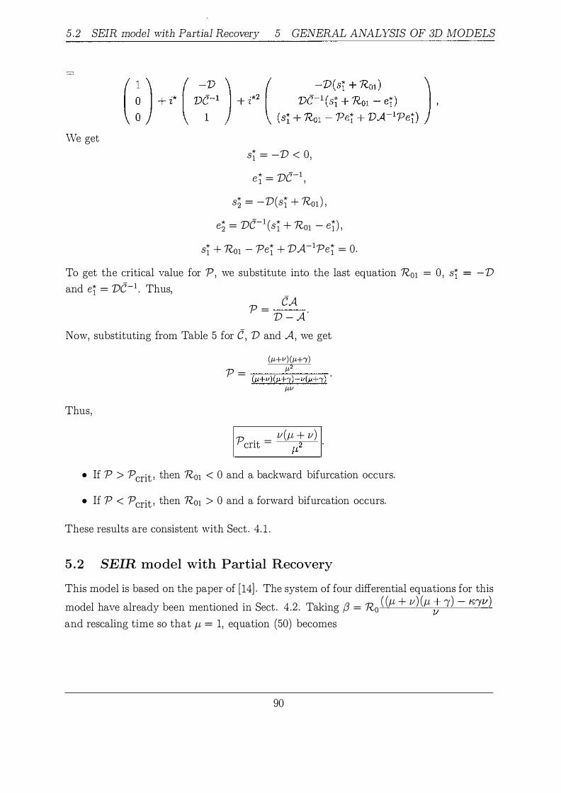
5.2 SEIR model with Partial Recovery 5 GENERAL ANALYSIS OF 3D MODELS
We get s� = -V < 0,
e� = vc-1 ,
s; = -V(s� + Rm) ,
e; = vc-1 (s� + Ro1 - e�) ,
s� + Ro1 - Pe� + VA-1Pe� = 0 .
To get the critical value for P, we substitute into the last equation R01 = 0 , s� = -V and et = vc-1 . Thus,
P = CA V - A
Now, substituting from Table 5 for C, V and A, we get
Thus,
(J-L+ V) (J-L+/) J-L2 p = (J-L+v)(J-L+'Y)-v(J-L+i) •
J-LV
p . _ v(p, + v) cnt - f-L'2 ·
• If P > P crit , then R01 < 0 and a backward bifurcation occurs.
• If P < P crit , then Ro1 > 0 and a forward bifurcation occurs.
These results are consistent with Sect . 4. 1 .
5 . 2 SEIR model with Partial Recovery
This model is based on the paper of [14] . The system of four differential equations for this model have already been mentioned in Sect . 4 .2 . Taking f3 = R0 ( (p, + v) (p, t !) - f"Jll) and rescaling time so that p, = 1, equation (50) becomes
90

5.2 SEIR model with Partial Recovery 5 GENERAL ANALYSIS OF 3D MODELS
Three Dimensional Exogenous Infection :Model ( SEIR model)
s* = 1 + is1 + i2*S2, Ro = 1 + i"R01 + i2"Rm - - - � - - - - - � - - - - - - ·
* s Rol < 0
Figure 58: An enlarged top-center portion of Fig. 26. In this sketch, it is clearly shown that st < 0 , and 7?01 < 0 give backward bifurcation, while 7?01 > 0 give forward bifurcation.
ds dt de dt di dt
1 - R0Esi - s,
R0Esi - PR0E(s + e + i)i - Ce + PR0Di + B(1 - PR0)i , c . �e - Az D '
where B = 7J-, E = D - B. (see Table 5) . We rewrite this equation in a ODE system
(65) by setting y = ( : ) . :re ( � �C -PROD - �(1 - PRo) ) , j (y) =
0 - D A ( s�·*
: ) At the steady state, y* = " solves
y* = ]\IJ-1 f(y*)
91
( 1 - R0Esi ) R0Esi - PR�E( s + e + i ) i .
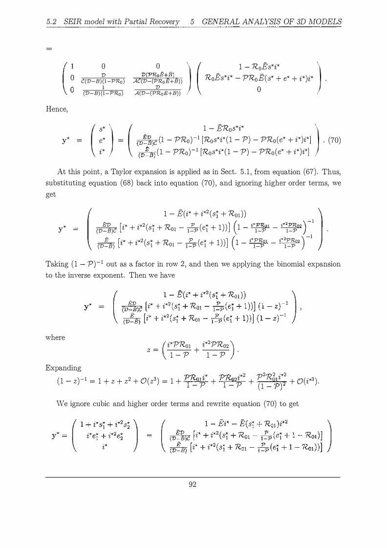
5.2 SEIR model with Partial Recovery 5 GENERAL ANALYSIS OF 3D MODELS
Hence,
0 V
C(V-B) (1-PRo) 1 (V-B) (1-PRo)
0 V(PRoE+B) AC(V-(PRoE+B)) V
A(V-(PRoE+B)) ) ( 1 - R0Es*i* ) RoEs*i* - PR0:(s* + e* + i*)i* .
( s* ) ( 1 - ERos*i* ) y* = e* = (v��)c (1 - PRo)-1 [Ros*i* ( 1 - P) - PRo( e* + i*)i*] . (70) i* (V�B) ( 1 - PRo)-1 [Ros*i* (1 - P) - PRo(e* + i*)i*]
At this point , a Taylor expansion is applied as in Sect. 5 . 1 , from equation (67) . Thus, substituting equation (68) back into equation (70) , and ignoring higher order terms, we get
y* -
1 - E(i* + i*2 (s� + R01 ) ) EV [i* + i*2 (s* + R _ _E_(e* + 1 ) ) ] (1 - i*PRo1 _ i*2PRo2 ) -1
(V-B)C 1 01 1-P 1 1-P 1-P __lL [i* + i*2 (s* + R _ _E_(e* + 1) )] (1 - i*PRo1 _ i*2PRo2 ) -1 (V-B) 1 01 1-P 1 1-P 1-P
Taking ( 1 - P)-1 out as a factor in row 2 , and then we applying the binomial expansion to the inverse exponent. Then we have
where
Expanding
( i*PRm i*2PRo2 ) Z = + . 1 - P 1 - P
Pn .* pn -*2 p2n2 ·*2 ( 1 - z)-1 = 1 + z + z2 + O(z3) = 1 + ''-'ol' l + '"02z + 01 z + O(i*3 ) 1 - P 1 - P (1 - P)2 .
We ignore cubic and higher order terms and rewrite equation (70) to get
92

5.2 SEIR model with Partial Recovery 5 GENERAL ANALYSIS OF 3D MODELS
Hence comparing equal powers of the perturbation variable i* to find the critical value for P.
We have
-E EV
(V -_B)C E
(V - B)
-E(st + Rol )
(VDE� B)C [st + Ro1 - /!_p (et + 1 - R01 ) ]
(V � B) [st + R01 - 1�p (et + 1 - Rol) ]
s� = -E < 0 ,
EV * e1 = (V - B)C '
E V - B = 1 '
s; = -E(s� + R01 ) ,
* EV [ * p ( * )] e2 = (V _ B)C sl + Ro1 - 1 _ p e1 + 1 - Ro1 ,
(V� B) [ s� + R01 - 1 � p ( e� + 1 - R01 ) l = 0 .
At the critical value for P, set R01 = 0 , st = -E and et = �· Thus we solve st + Ro1 - 1�p (et + 1 - R01 ) = 0 to get Pcrit
EC Pcrit = EC - V - C
Substituting from Table 5 , the values for C, V and E, we get
• If P > P crit then Ro1 < 0 and a backward bifurcation occurs.
• If P < P crit then R01 > 0 and a forward bifurcation occurs.
These results are consistent with Sect. 4 .2 .
93

5.3 SEIR model with Full Recovery 5 GENERAL ANALYSIS OF 3D MODELS
SEIR model witlt partial rccot,ery
s*=:t+i'·s"+i*2 s•· Ro = 1+ i'R +i''2R t 2 ' 01 02
R01 > o
Figure 59: Enlarged top-center portion of Bifurcation diagram 32. The critical value P . _ (J-L + 1) (J-L + v) - rqv
cnt - v/( 1 _ t�,)
5 . 3 SEIR model with Full Recovery
This model is based on the paper of [14] . The system of four differential equations for this model are already mentioned in Sect . 4.3. The basic reproduction number R0 is same as in Sect . 4. 1 . Thus rescaling time so that 11 = 1 , equation (54) becomes
ds dt de dt
1 - R0'Dsi - s ,
R0'Dsi - PR0'D(1 - s - e - i)i - Ce, di C- A . - -=e - z . dt 'D
See Table 5 for notations. We write this equation in a matrix framework system (65) by
setting y = ( ; ) ( 1 0 Here ]V! = 0 C
C 0 - 'D
-P:oD ) , j (y) = ( 1 - R0'Dsi ) R0'Dsi - PR�D(s + e + i)i .
At the steady state y* = ( ;: ) , we have
94

5.3 SEIR model with Full Recovery 5 GENERAL ANALYSIS OF 3D MODELS
Hence,
0 1
C(l-PRo ) 1 D(l-PRo)
y* = M-1 j (y*)
0 PRo V * ·* * * ·* ·* ) ( 1 - R0Ds*i* ) AC(l�PRo) RoDs z - PRo:(s + e + z )z .
A(l-PRo)
( s* ) ( 1 - DR0s*i* ) y* = e* = ve-1 (1 - PR0)-1 [R0s*i* (1 - P) - PR0(e* + i*)i*] . (71) i* (1 - PR0)-1 [R0s*i* (1 - P) - PRo(e* + i*)i*]
In equation (67) , we apply a Taylor expansion using the perturbation variable i* . Substituting equation (68) back into equation (71 ) , we get
1 - D(i* + i*2 (st + Rol ) )
Y* ve-l [i* + i*2 (s* + R - _E_(e* + 1) )] (1 - i*PRm - i*2PRo2) -1 1 01 1-P 1 1-P 1-P
[i* + i*2 (s* + J? _ _E_ (e* + 1 ) )] (1 - i*PRo1 _ i*2PRo2 ) -l 01 1-P 1 1-P 1-P
Again, as in Sect . 5 .2 , we apply a binomial expansion
substituting z into y* to have
( i*PR01 i*2PRo2 ) Z = + . 1 - P 1 - P
( 1 - D(i* + i*2 (st + R01 ) ) ) y* = ve-l [i* + i*2 (st + R01 - 1�p (et + 1) ) ] ( 1 - z)-1
[i* + i*2 (st + R01 - 1�p (et + 1 ) )] ( 1 - z)-1
Expanding ( 1 - z)-1 = 1 + z + z2 + O(z3 ) and ignoring cubic and higher order terms, we rewrite equation (71) to get
( 1 - Vi* - D(st + R01 )i*2 ) ve-l [i* + i*2 (st + R01 - 1�p (et + 1 - R01 )] [i* + i*2 (st + R01 - 1�p (et + 1 - R01 ) )]
Comparing equal powers of the perturbation variable i* , we have
95

5.3 SEIR model with Full Recovery 5 GENERAL ANALYSIS OF 3D MODELS
We get s� = -D < 0 ,
* D el = C ' s; = -D(s� + R01 ) ,
e; = � [s� + R01 - 1 �p (e� + 1 - Roi )l ,
s� + R01 - pp (e� + 1 - Roi ) = 0. 1 -
At the critical value of P, set R01 = 0 , st = -D and et = � - Thus we solve st + R01 -1�p (et + 1 - Rm ) = 0 for Pcrit ·
DC p crit = DC - D - C
From Table 5 , we substitute the values for C and D
Thus,
p . - (,u + V? (,u + ')') cnt - (,u + v)2 (,u + 'Y) _ ,u(,u + v) _ ,uv(,u + v)
I p . = (,u + 'Y) (,u + V) I cnt V')'
• If P > P crit then Rm < 0 and a backward bifurcation occurs.
• If P < Pcrit then Rm > 0 and a forward bifurcation occurs.
These results are consistent with Sect . 4.3 .
96

5.4 The SIR Model with Carrier Class 5 GENERAL ANALYSIS OF 3D MODELS
SEIR model witlt.full recot•ery
S·' =:J.+i*·s*+i"'2 s"· Ro = :1.+ i "R +i*2R l 2 ' 0:1. 02
Figure 60: Blow up of the bifurcation diagram 38. Labels are as in Fig. 26. The critical value of P for this class is P · = (p, + I) (p, + z;) cnt Zl/ ·
5 . 4 The SIR Model with Carrier Class
Consider the ordinary differential equations (57) , as discussed in Sect. 4.4. Rescaling time so that p, = 1 , equations (57) become
ds dt di dt de dt
1 - xs - s
xs - Ai
See Table 5 for notation. We know from Sect . 4.4 that q(x) is a function of x. If we
rewrite this in a matrix framework system (65) by setting y = ( ! ) , then we have
( 1 0
M = 0 A 0 0
0 ) ( 1 - xs ) 0 ' J (y) = xs . B q(x)/J,i
97
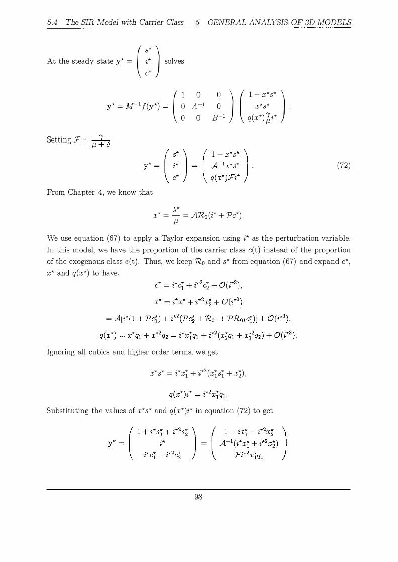
5.4 The SIR Model with Carrier Class 5 GENERAL ANALYSIS OF 3D MODELS
At the steruly state y* = ( :: ) solves
y* = Jvi-1f(y*) = ( � Ao 1 � ) 0 � B-1
Setting :F = M t ()
From Chapter 4, we know that
( 1 - x*s* ) x*s* . q(x*)'f;i*
)..* x* = - = AR0 (i* + Pc*) . M
(72)
We use equation (67) to apply a Taylor expansion using i* as the perturbation variable. In this model, we have the proportion of the carrier class c( t) instead of the proportion of the exogenous class e( t) . Thus, we keep 7?0 and s* from equation ( 67) and expand c* , x* and q(x*) to have.
Ignoring all cubics and higher order terms, we get
x* s* - i*x* + i*2 (x* s* + x*) - 1 1 1 2 l
Substituting the values of x* s* and q(x*)i* in equation (72) to get
98

5.4 The SIR Model with Carrier Class 5 GENERAL ANALYSIS OF 3D MODELS
or
where, x� = A(1 + Pc�) ,
x; = A(Pc; + Rm + PRole�) .
We now substitute the values of xt and x2 and comparing equal powers of i* to have
s� = -x� = -A(1 + Pc�) < 0 ,
c� = 0 ,
s; = -A[(1 + Pc�)s� + Pc; + R01 + PRmc�] ,
0. (73)
At the critical value for P, R01 = 0 , and substituting values st , et and c; , equation (73) becomes
We know that :F = f-l � (5 , hence
p = _1_ .
:Fql
• If P > P crit then Rm < 0 and a backward bifurcation occurs.
• If P < Pcrit then R01 > 0 and a forward bifurcation occurs.
These results are consistent with Sect . 4.4 . This concludes that a backward bifurcation occurs when Rm < 1 , and for R01 > 1 , a forward bifurcation occurs. These results are consistent with the carrier class given in Sect . 4.4 , and are only valid when q(O) = 0 and q' (O) = q1 > 0 (as discussed in Sect. 4 .4) . This general analysis only works for functions such as
99

5.4 The SIR Model with Carrier Class 5 GENERAL ANALYSIS OF 3D MODELS
Carrier Class
s'· = 1 + is1 + p*s2, Ro = 1 + i'"Rm + P"'Ro2
Rol < 0 ' • ' • . . .
Figure 6 1 : A top-center blow up of Bifurcation diagram 44. Labels are as in Fig. 26 . The "t " l l f p . p f-L + 6 en 1ca va ue or 1s crit =
' ( * ) . /q X
100

6 DISCUSSION
6 Discussion The infection-free steady state, in the renowned SIR endemic model, is globally stable for R0 < 1 and unstable for R0 > 1 . This gives rise to a forward bifurcation at Ro = 1 .
Asymptotic stability in the SIR endemic model shows that there is an infection that persists endemically when R0 > 1 . We considered the basic reproduction number Ro as a main bifurcation parameter, which has been used to determine the stability of the steady states of the SIR endemic model. In this thesis we mainly focused on the two and three dimensional extensions, of the SIR endemic model, for which a backward bifurcation occurs at R0 = 1 . For this we chose some reasonable biological factors that lead to the phenomena of the backward bifurcation, multiple endemic steady states and hysteresis with some parameter values. We applied analytical and numerical tools to investigate these phenomena.
Furthermore we presented a general classification of the two and three dimensional extensions of the SIR endemic model in which we expanded steady state solutions, in terms of a small perturbation variable i* . We used Taylor and Binomial expansions in order to establish a matrix framework. Moreover , we showed that the results given in the general classification are consistent with the results deduced in the qualitative approach.
Accordingly in Chapter 1 , we gave a brief background of the SIR model and its two main examples i .e . the SIR epidemic model and the SIR endemic model. In two short segments Sect . 1 . 2 and Sect. 1 . 3 we discussed these examples. We also studied and reproduced the bifurcation analysis which is done in [ 12] . In Sect. 1 .2 , we briefly looked at the SIR epidemic model while in the Sect . 1 . 3 we thoroughly investigated the steady state solutions, their stability and their phase-plane analysis. The purpose of this thesis is to closely investigate the SIR endemic model and its extensions.
In the extended models we used P as a secondary bifurcation parameter, whose precise definition differs between the models. In Chapter 2, we examined two dimensional extensions of the SIR endemic model which are: the SIR with a susceptible R class (Sect . 2 . 1 ) ;
non-linear transmission (Sect . 2 .2) ; and exogenous infection (Sect. 2.3) . We classified these models in five steps. Firstly we used a Dulac's criteria to rule out limit cycles and then we evaluated the steady state solutions of these models by setting the right-hand side of the differential equations to zero. Then we found the critical value for P and a saddle node equation of R0 which solved for Rsaddle ' the minimum value of R0 for which a steady state exists. Thirdly, we linearised the system to find the local stability of these steady state solutions. We used PPLANE, the numerical program of MATLAB [ 10] to
101

6 DISCUSSION
plot bifurcation and phase-plane diagrams for a variety of parameter values given in each
section. We analysed bifurcations and the phase-planes using a threshold parameter 1?0
and a secondary parameter P, adopting the idea from [12] . The secondary parameter P has different definition for each model.
In Sect . 2 . 1 , we studied a model from [13] . We found that, for 1?0 > 1 , a forward bifur
cation exists at 1?0 = 1 , when there is an unstable infection-free steady state and a unique
endemic steady state independent of P . A backward bifurcation occurs, when a stable
infection-free steady state and multiple endemic steady states exist for Rsaddle < Ro < 1
and P > Pcrit · This also causes the hysteresis phenomenon.
Usually it is assumed that with nonlinear transmission, we find only a forward bifurca
tion. Instead we discovered in Sect. 2 .2 , a function h( i) that depends on the infectives and
satisfies certain biological conditions. We also used a theorem from the paper of Games
[6] that fails to prove the existence of any limit cycle for this function. We also observed
that this model exhibits a backward bifurcation and hysteresis phenomena.
In Sect . 2 . 3 , we have investigated a model , introduced by [4] , in which the recovered
class is replaced from the exposed class. This model also exhibited the backward bifurca
tion phenomenon.
Now, in Chapter 3 , we applied a general classification for the two dimensional exten
sions of the SIR endemic model. We investigated the different dynamics applying Taylor
and Binomial expansions by a perturbation variable i* near the bifurcation point i .e . near
1?0 = 1 . We checked if the results at the turning points are consistent with the results
found in Chapter 2 .
Chapter 4 took account of three dimensional extensions of the SIR endemic model.
We considered the same strategy as in Chapter 2 except for the following: we cannot use
Dulac's criteria with the three dimensional differential equations; we linearised the 3 x
3 Jacobian matrices using Maple [5] ; we checked the stability using the Routh-Hurwitz
Criteria; and we used ODE45 , a numerical package of MATLAB [ 10] , to plot phase
plane diagrams. These phase-planes plotted, by putting three dimensions onto the two
dimensional projection, hence the trajectories may appear to coincide. We studied four
three dimensional extensions: SEIR model (Sect . 4 . 1 ) ; SEIR model with full recovery
class (Sect . 4 .2) ; SEIR model with partial recovery class (Sect . 4 .3) ; and SIR model with
a carrier class (Sect . 4 .4) .
102

6 DISCUSSION
In Sect . 4 . 1 , Sect . 4 .2 , Sect. 4 .3 , the models are similar to the two dimensional SIR model with exogenous infection in Sect . 2 .3 . These models have a recovered class as well
as the exposed class. Sections 4 .2 and 4.3 were proposed in a paper by [14] . We checked
with our qualitative approach that these models are consistent with the techniques used
in [14] . We also proved that these models exhibit backward bifurcation.
In Sect . 4 .4, we considered a carrier class instead of exogenous class. In this model
we had a proportion q(x) which is a function of x = f3(i+'Pc) that become carriers. We as-J.L sumed that for q(x) = 0 , q'(x) 2': 0 when x 2': 0 . This assumption led to the two examples
of carrier class; Example 1 had a function q(x) = 1 - e0·9x and; Example 2 had a function
q(x) = x;:2 . Example 1 exhibited the same phenomenon i .e . backward bifurcation occurs
at R0 = 1 as in Sect . 4. 1 , Sect . 4 .2 , Sect . 4 .3 . On the other hand, Example 2 exhibited
two backward bifurcations. The bifurcation at R0 = 1 is forward but the locus of steady
state turns backward for some R0 > 1 .
Lastly in Chapter 5 , we have a similar general classification for three dimensional ex
tensions as in Chapter 3 . We found that these models are consistent with the results we
had deduced in Chapter 4. In Sect. 5 .4 , we showed that the results are compatible only
for certain function q(x) such as in Example 1 .
Finally we conclude that the calculations contained in this thesis will b e useful in
developing an understanding of both numerical and analytical methods using MATLAB
[ 10] and Maple [5] respectively, and our results in Chapters 2 and 4 are consistent with
those in Chapters 3 and 5 .
103
REFERENCES REFERENCES
References [1] Diekmann, 0 . , J. A. P. Heesterbeek. 2000 . Mathematical epidemiology of infectious
disease: model building) analysis and interpretation. Wiley series in mathematical
and computational biology. Wiley, Chichester , UK.
[2] Edelstein-Keshet , 1. 2005 . Mathematical Models in Biology. Society for Industrial
and Applied Mathematics, Philadelphia PA.
[3] Ellner, S . P. and J . Guckenheimer. 2006. Differential equation models for infectious
disease. Princeton University Press, Princeton, NJ.
[4] Feng, Z. , C. Castillo-Chavez and A. F. Capurro. 2000. A Model for tuberculosis with
exogenous reinfection. Theoretical Population Biology 57: 235-247.
[5] Garvan, Frank. 2001 . The Maple Book. Chapman & Hall/CRC Press. http : I /www . rnaplesoft . corn (accessed November 28, 2001 ) .
[6] Games, M . G . M. , A . Margheri, G . F . Medley and C . Rebelo. 2005. Dynamical
behaviour of epidemiological models with sub-optimal immunity and nonlinear inci
dence. Journal of Mathematical Biology 51 : 414-430 .
[7] Kermack, W. 0. and A. G . McKendrick. 1927. A Contribution to the mathematica:
theory of epidemics I. Proc. Roy. Soc. London A115 : 700-721 .
[8] Korobeinikov, A. 2001 . Stability and Bifurcation of Deterministic Infectious Disease.
ResearchSpace@A uckland.
[9] Medley, G . F. , N . A. Lindop, W. J . Edmunds and D . J . Nokes. 2001 . Hepatitis-B virus
endemicity: heterogeneity, catastrophic dynamics and control. Nature Medicine. 5 :
619-624.
[10] Moler, Cleve B. 2004. Numerical Computing with MATLAB. Cambridge University
Press. http : I lwww . rnathworks . corn (accessed January 1 , 2004) .
[ 1 1 ] Rhodes, A. J . and E. S . Allman. 2004. Mathematical Models in Biology: An Intra-
duction. Cambridge University Press, Cambridge, UK.
[12] Roberts, M. G. 2007. The pluses and minuses of R0 . Journal of the Royal Society
Interface 4: 949-961 .
[13] Safan, M. , J . A. P. Heesterbeek and K. Dietz. 2006. The minimum effort required
to eradicate infections in models with backward bifurcation. Journal of Mathemati
cal Biology 53: 703-718.
104

REFERENCES REFERENCES
[14] van den Driessche, P. and J . Watmough. 2002. Reproduction numbers and sub
threshold endemic equilibria for computational models of disease transmission. Math
ematical Biosciences 180: 29-48.
105
Copyright is owned by the Author of the Thesis. Permission is given for a copy to
be downloaded by an individual for the purpose of research and private study only. This
theisi may not reproduced elsewhere without the permission of the Author.

"Ji". '\.1 MasseyUniversity
Declaration Confirming Content of Digital Version of Thesis
I confirm that the content of the d ig ita l version of this thesis
is the final amended version fol lowi ng the examination process and is identica l to this hard bound paper copy.
Student's Name:
Student's Signature:
Date: