Baja/FSAE Templates – Half Car Models User Guide

Introduction Multi-body dynamics is a powerful tool that can be used in the development of the vehicle systems

like the suspensions, steering systems and the brake systems. Clear understanding of vehicle

dynamics and powerful tools to simulate design ideas and design experiments can provide the user

with the extra competitive edge to its rivals.

This document gives the user a brief introduction to Muti-body dynamics followed by an easy step

by step process the user can follow to model and simulate half car models to observe changes and

impact on handling the vehicle can have based on their design decisions.

Multi-body Dynamics Multi-body Dynamics based simulations deals with simulations involving large displacements. “Multi-

body” implies that multiple bodies interact in the simulation. “Dynamics” implies that the

simulations determine the forces and moments acting between bodies and compute displacements

of the bodies based on these and other constraints applied on the bodies.

Motion View in the Hyper Works suit of design tools is the Multi-body Dynamics pre-processor while

Motion Solve is the multi-body dynamics solver. For more information about Multi-body dynamics

and other details the Motion View help, reference guide and tutorials can be used.

The Baja and Formula Student “templates” available for simulation for Motion View are designed for

the use of a user who has some basic knowledge of kinematics and dynamics of suspension systems.

Due to their simplicity and abstraction, the templates can be used by someone not very conversant

with Motion View as a pre-processor but some basic knowledge about the pre processor will

definitely aid the user in having a better understanding and allow the user to explore more detailed

advanced simulations.

Rigid Body Dynamics A multi-body dynamics simulation where all the bodies modelled as rigid or inflexible bodies is a rigid

body dynamics simulation. Although Altair’s Multi-Body Dynamics simulation products do support

modelling of flexible bodies into the simulation, rigid body simulations are always the starting point.

Vehicle Models in Multi-Dynamics Vehicle models in Multi-body dynamics involve modelling the different “moving” components as

bodies and the connections between them as joints or constrains. A detailed look at the templates

will show the user how the individual components of the suspension and steering is modelled. The

templates for Baja and FSAE are developed to abstract this information from the user, but it is

always helpful and worthwhile to look at the details to understand the simulation.

Half Car Model

Introduction Half car models in terms of Multi-body dynamics involve the modelling of the following sub-systems

of the vehicle

Suspension

Steering (front)

Drive shafts (if driven wheels)

These sub-systems are typically defined by what are called the suspension “hard points”. These are 3

dimensional coordinates in space where the different suspension components connect to the

chassis, wheels and on another. They define the geometry of the suspension you choose which

eventually determine the kinematics and the dynamics of the suspension systems.

Setting up half car models The half car models are available as a part of the Baja/FSAE templates that are provided on the Altair

Website.

There are 2 options to build a half car vehicle

Load the generalised half vehicle model and make modifications to it directly. Changes in

suspension type or steering type are done by replacement.

Assemble a half car model by adding the subsystems one by one. This gives the freedom to

choose any type of suspensions from the beginning of the model set-up.

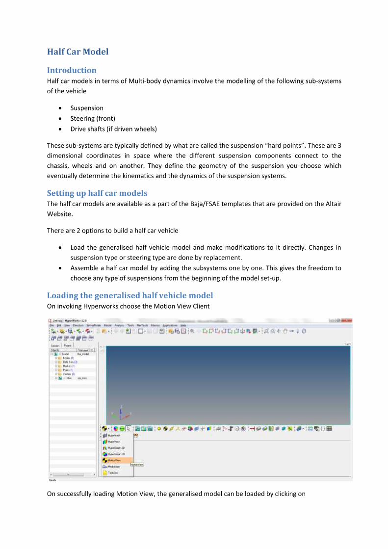
Loading the generalised half vehicle model On invoking Hyperworks choose the Motion View Client

On successfully loading Motion View, the generalised model can be loaded by clicking on

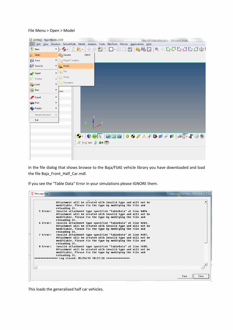
File Menu > Open > Model

In the file dialog that shows browse to the Baja/FSAE vehicle library you have downloaded and load

the file Baja_Front_Half_Car.mdl.

If you see the “Table Data” Error in your simulations please IGNORE them.

This loads the generalised half car vehicles.

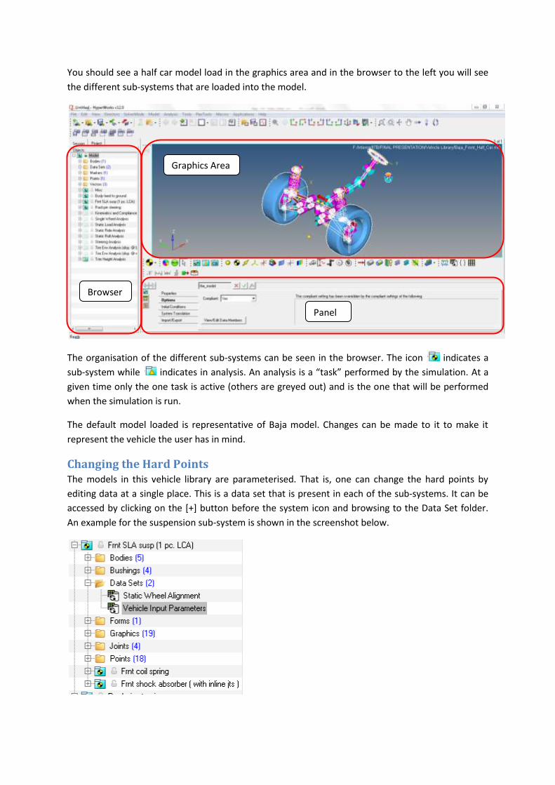
You should see a half car model load in the graphics area and in the browser to the left you will see

the different sub-systems that are loaded into the model.

The organisation of the different sub-systems can be seen in the browser. The icon indicates a

sub-system while indicates in analysis. An analysis is a “task” performed by the simulation. At a

given time only the one task is active (others are greyed out) and is the one that will be performed

when the simulation is run.

The default model loaded is representative of Baja model. Changes can be made to it to make it

represent the vehicle the user has in mind.

Changing the Hard Points The models in this vehicle library are parameterised. That is, one can change the hard points by

editing data at a single place. This is a data set that is present in each of the sub-systems. It can be

accessed by clicking on the [+] button before the system icon and browsing to the Data Set folder.

An example for the suspension sub-system is shown in the screenshot below.

Browser

Graphics Area

Panel

Clicking on this loads the Data Set panel in the panel area. Here the values of the hard points and

other parameters can be changed. The button at the far right of the panel will pop-out the lost

of parameters that can be changed. For basic preliminary simulations changing these parameters

only would be sufficient.

Adding/Removing sub-systems Sub-systems in the vehicle library are interchangeable which means that they can be replaced by

other types of the same sub-system. In the example below, the front double SLA suspension is

replaced by a push-rod type suspension.

A sub-system can be removed from the model by simply right clicking on the model tree to invoke

the context menu and choose the “Delete” option.

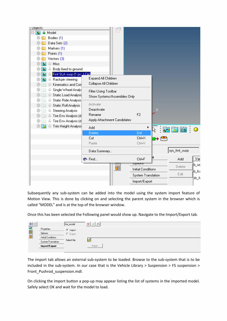
Subsequently any sub-system can be added into the model using the system import feature of

Motion View. This is done by clicking on and selecting the parent system in the browser which is

called “MODEL” and is at the top of the browser window.

Once this has been selected the Following panel would show up. Navigate to the Import/Export tab.

The import tab allows an external sub-system to be loaded. Browse to the sub-system that is to be

included in the sub-system. In our case that is the Vehicle Library > Suspension > FS suspension >

Front_Pushrod_suspension.mdl.

On clicking the import button a pop-up may appear listing the list of systems in the imported model.

Safely select OK and wait for the model to load.

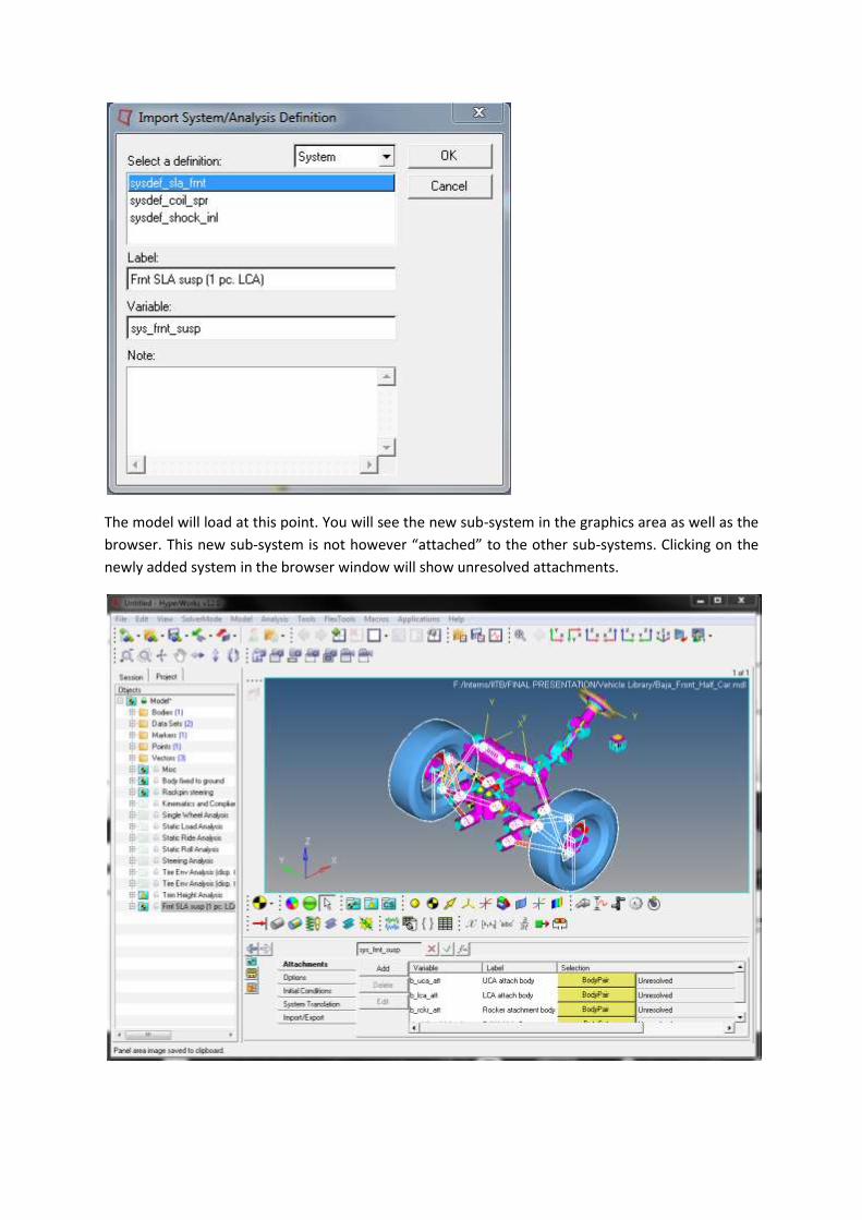
The model will load at this point. You will see the new sub-system in the graphics area as well as the

browser. This new sub-system is not however “attached” to the other sub-systems. Clicking on the

newly added system in the browser window will show unresolved attachments.

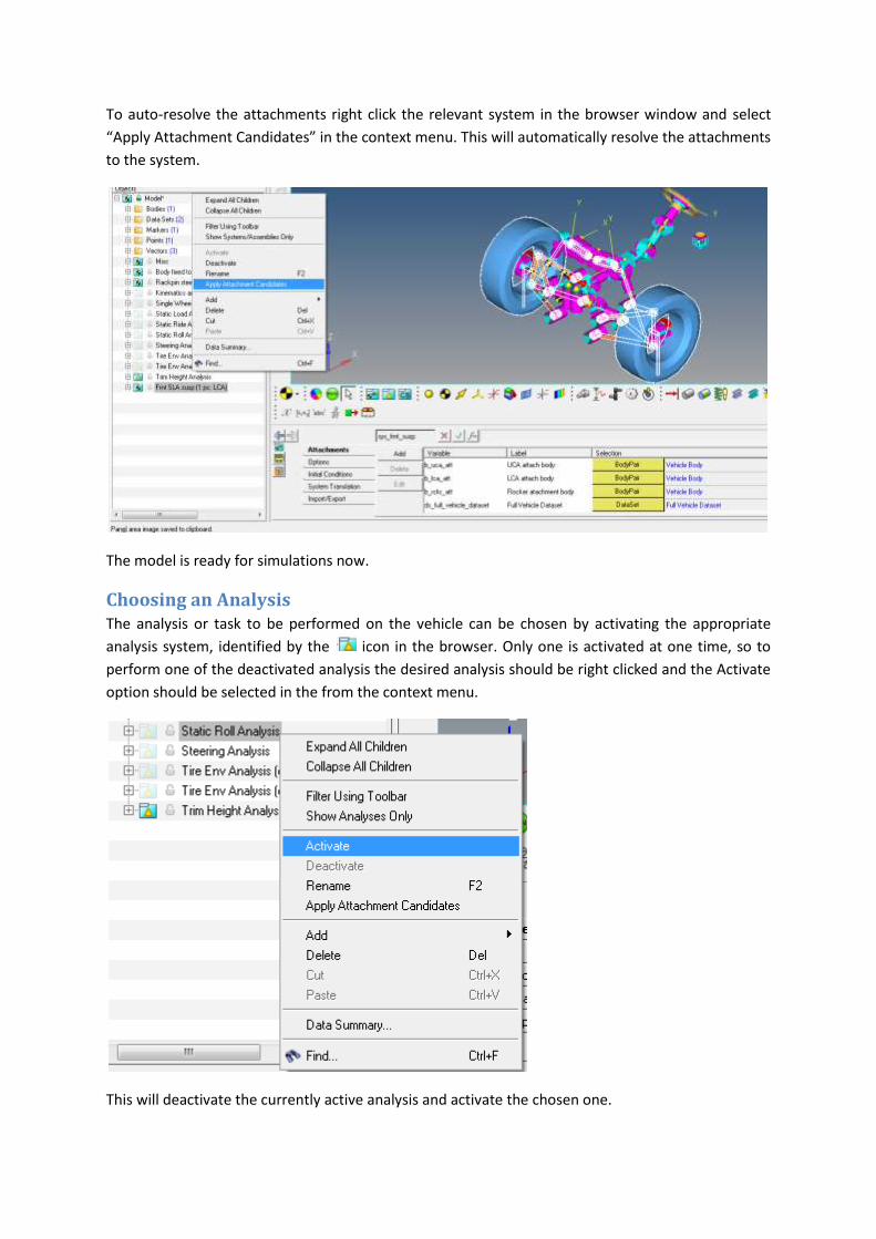
To auto-resolve the attachments right click the relevant system in the browser window and select

“Apply Attachment Candidates” in the context menu. This will automatically resolve the attachments

to the system.

The model is ready for simulations now.

Choosing an Analysis The analysis or task to be performed on the vehicle can be chosen by activating the appropriate

analysis system, identified by the icon in the browser. Only one is activated at one time, so to

perform one of the deactivated analysis the desired analysis should be right clicked and the Activate

option should be selected in the from the context menu.

This will deactivate the currently active analysis and activate the chosen one.

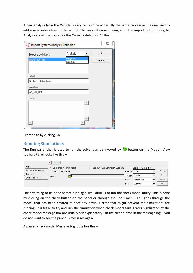
A new analysis from the Vehicle Library can also be added. By the same process as the one used to

add a new sub-system to the model. The only difference being after the import button being hit

Analysis should be chosen as the “Select a definition:” filter

Proceed to by clicking OK.

Running Simulations

The Run panel that is used to run the solver can be invoked by button on the Motion View

toolbar. Panel looks like this –

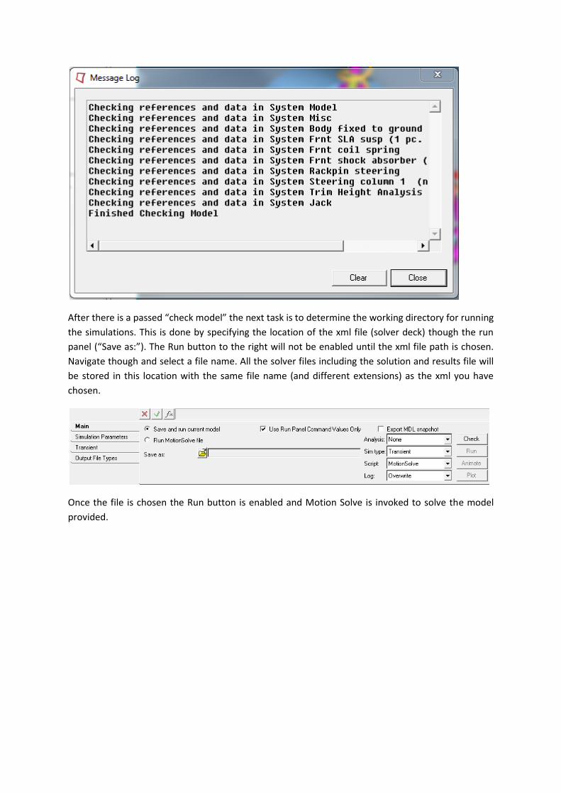
The first thing to be done before running a simulation is to run the check model utility. This is done

by clicking on the check button on the panel or through the Tools menu. This goes through the

model that has been created to spot any obvious error that might prevent the simulations are

running. It is futile to try and run the simulation when check model fails. Errors highlighted by the

check model message box are usually self explanatory. Hit the clear button in the message log is you

do not want to see the previous messages again.

A passed check model Message Log looks like this –

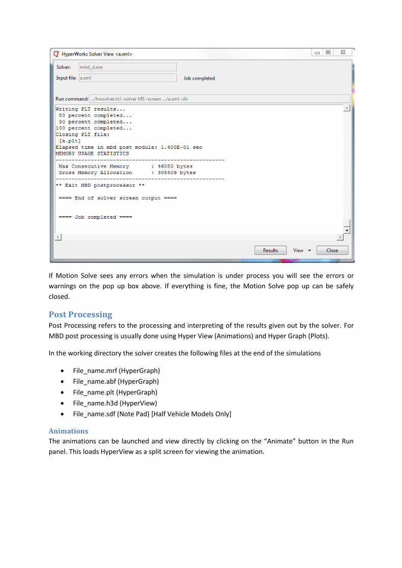
After there is a passed “check model” the next task is to determine the working directory for running

the simulations. This is done by specifying the location of the xml file (solver deck) though the run

panel (“Save as:”). The Run button to the right will not be enabled until the xml file path is chosen.

Navigate though and select a file name. All the solver files including the solution and results file will

be stored in this location with the same file name (and different extensions) as the xml you have

chosen.

Once the file is chosen the Run button is enabled and Motion Solve is invoked to solve the model

provided.

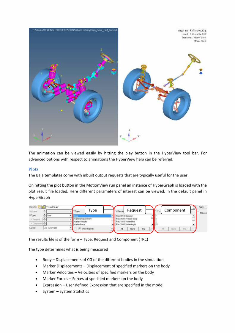
If Motion Solve sees any errors when the simulation is under process you will see the errors or

warnings on the pop up box above. If everything is fine, the Motion Solve pop up can be safely

closed.

Post Processing Post Processing refers to the processing and interpreting of the results given out by the solver. For

MBD post processing is usually done using Hyper View (Animations) and Hyper Graph (Plots).

In the working directory the solver creates the following files at the end of the simulations

File_name.mrf (HyperGraph)

File_name.abf (HyperGraph)

File_name.plt (HyperGraph)

File_name.h3d (HyperView)

File_name.sdf (Note Pad) [Half Vehicle Models Only]

Animations

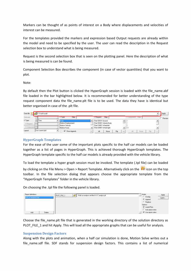
The animations can be launched and view directly by clicking on the “Animate” button in the Run

panel. This loads HyperView as a split screen for viewing the animation.

The animation can be viewed easily by hitting the play button in the HyperView tool bar. For

advanced options with respect to animations the HyperView help can be referred.

Plots

The Baja templates come with inbuilt output requests that are typically useful for the user.

On hitting the plot button in the MotionView run panel an instance of HyperGraph is loaded with the

plot result file loaded. Here different parameters of interest can be viewed. In the default panel in

HyperGraph

The results file is of the form – Type, Request and Component (TRC)

The type determines what is being measured

Body – Displacements of CG of the different bodies in the simulation.

Marker Displacements – Displacement of specified markers on the body

Marker Velocities – Velocities of specified markers on the body

Marker Forces – Forces at specified markers on the body

Expression – User defined Expression that are specified in the model

System – System Statistics

Type Request Component

Markers can be thought of as points of interest on a Body where displacements and velocities of

interest can be measured.

For the templates provided the markers and expression based Output requests are already within

the model and need to be specified by the user. The user can read the description in the Request

selection box to understand what is being measured.

Request is the second selection box that is seen on the plotting panel. Here the description of what

is being measured is can be found.

Component Selection Box describes the component (in case of vector quantities) that you want to

plot.

Note:

By default then the Plot button is clicked the HyperGraph session is loaded with the file_name.abf

file loaded in the bar highlighted below. It is recommended for better understanding of the type

request component data the file_name.plt file is to be used. The data they have is identical but

better organised in case of the .plt file.

HyperGraph Templates

For the ease of the user some of the important plots specific to the half car models can be loaded

together as a list of pages in HyperGraph. This is achieved thorough HyperGraph templates. The

HyperGraph template specific to the half car models is already provided with the vehicle library.

To load the template a hyper graph session must be invoked. The template (.tpl file) can be loaded

by clicking on the File Menu > Open > Report Template. Alternatively click on the icon on the top

toolbar. In the file selection dialog that appears choose the appropriate template from the

“HyperGraph Templates” folder in the vehicle library.

On choosing the .tpl file the following panel is loaded.

Choose the file_name.plt file that is generated in the working directory of the solution directory as

PLOT_FILE_1 and hit Apply. This will load all the appropriate graphs that can be useful for analysis.

Suspension Design Factors

Along with the plots and animation, when a half car simulation is done, Motion Solve writes out a

file_name.sdf file. SDF stands for suspension design factors. This contains a list of numerical

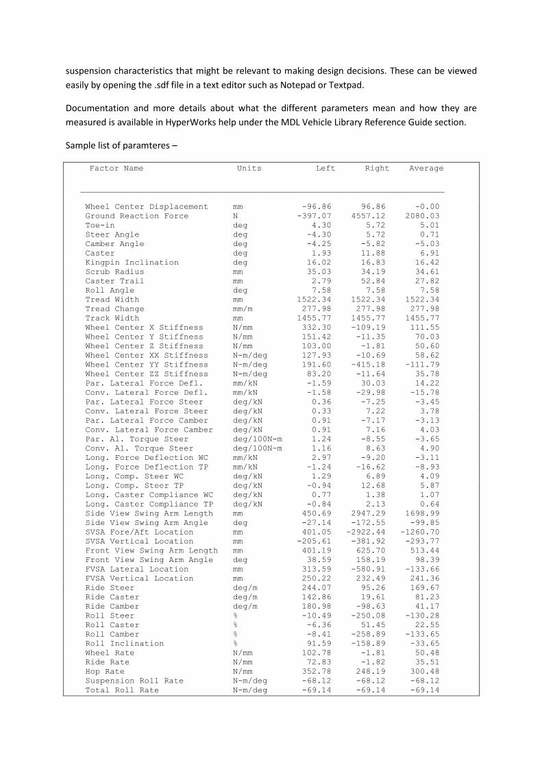
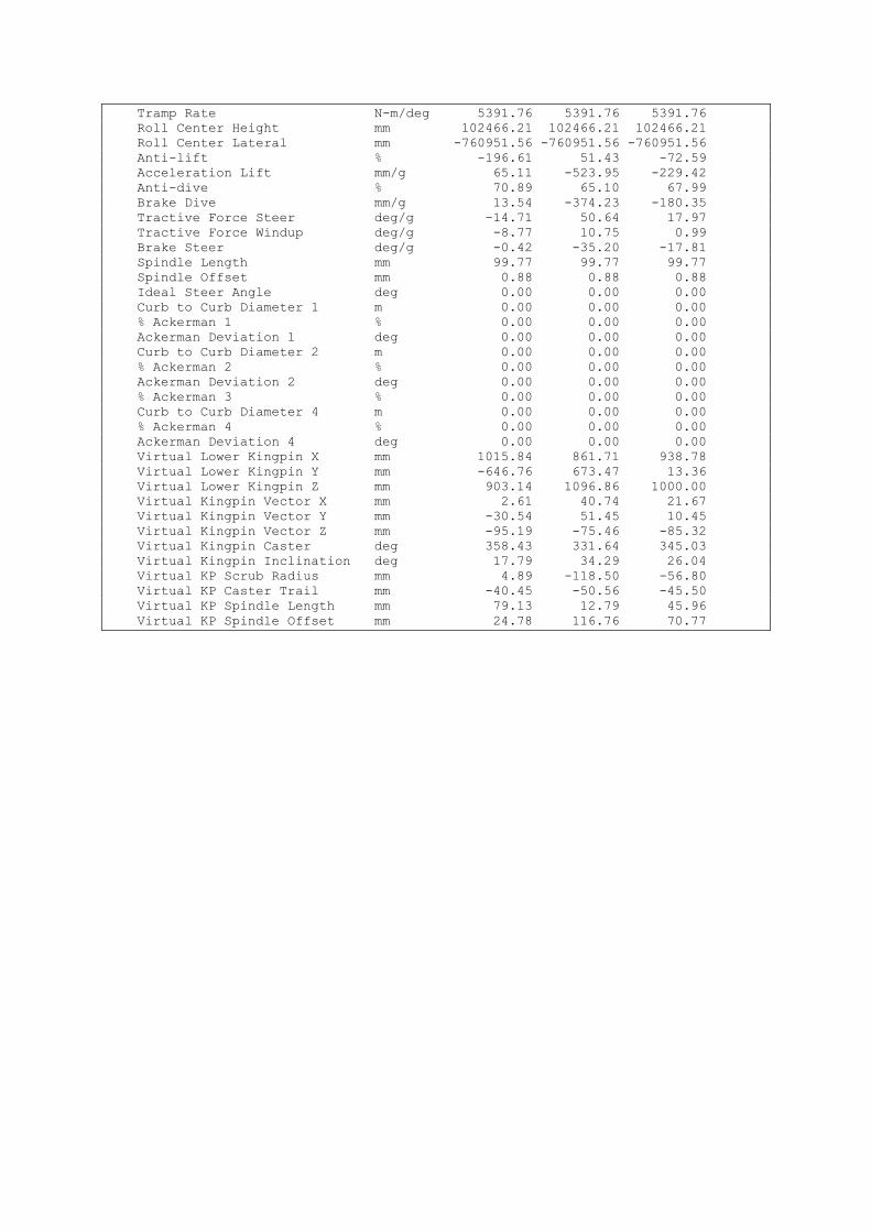
suspension characteristics that might be relevant to making design decisions. These can be viewed

easily by opening the .sdf file in a text editor such as Notepad or Textpad.

Documentation and more details about what the different parameters mean and how they are

measured is available in HyperWorks help under the MDL Vehicle Library Reference Guide section.

Sample list of paramteres –

Factor Name Units Left Right Average

__________________________________________________________________________

Wheel Center Displacement mm -96.86 96.86 -0.00

Ground Reaction Force N -397.07 4557.12 2080.03

Toe-in deg 4.30 5.72 5.01

Steer Angle deg -4.30 5.72 0.71

Camber Angle deg -4.25 -5.82 -5.03

Caster deg 1.93 11.88 6.91

Kingpin Inclination deg 16.02 16.83 16.42

Scrub Radius mm 35.03 34.19 34.61

Caster Trail mm 2.79 52.84 27.82

Roll Angle deg 7.58 7.58 7.58

Tread Width mm 1522.34 1522.34 1522.34

Tread Change mm/m 277.98 277.98 277.98

Track Width mm 1455.77 1455.77 1455.77

Wheel Center X Stiffness N/mm 332.30 -109.19 111.55

Wheel Center Y Stiffness N/mm 151.42 -11.35 70.03

Wheel Center Z Stiffness N/mm 103.00 -1.81 50.60

Wheel Center XX Stiffness N-m/deg 127.93 -10.69 58.62

Wheel Center YY Stiffness N-m/deg 191.60 -415.18 -111.79

Wheel Center ZZ Stiffness N-m/deg 83.20 -11.64 35.78

Par. Lateral Force Defl. mm/kN -1.59 30.03 14.22

Conv. Lateral Force Defl. mm/kN -1.58 -29.98 -15.78

Par. Lateral Force Steer deg/kN 0.36 -7.25 -3.45

Conv. Lateral Force Steer deg/kN 0.33 7.22 3.78

Par. Lateral Force Camber deg/kN 0.91 -7.17 -3.13

Conv. Lateral Force Camber deg/kN 0.91 7.16 4.03

Par. Al. Torque Steer deg/100N-m 1.24 -8.55 -3.65

Conv. Al. Torque Steer deg/100N-m 1.16 8.63 4.90

Long. Force Deflection WC mm/kN 2.97 -9.20 -3.11

Long. Force Deflection TP mm/kN -1.24 -16.62 -8.93

Long. Comp. Steer WC deg/kN 1.29 6.89 4.09

Long. Comp. Steer TP deg/kN -0.94 12.68 5.87

Long. Caster Compliance WC deg/kN 0.77 1.38 1.07

Long. Caster Compliance TP deg/kN -0.84 2.13 0.64

Side View Swing Arm Length mm 450.69 2947.29 1698.99

Side View Swing Arm Angle deg -27.14 -172.55 -99.85

SVSA Fore/Aft Location mm 401.05 -2922.44 -1260.70

SVSA Vertical Location mm -205.61 -381.92 -293.77

Front View Swing Arm Length mm 401.19 625.70 513.44

Front View Swing Arm Angle deg 38.59 158.19 98.39

FVSA Lateral Location mm 313.59 -580.91 -133.66

FVSA Vertical Location mm 250.22 232.49 241.36

Ride Steer deg/m 244.07 95.26 169.67

Ride Caster deg/m 142.86 19.61 81.23

Ride Camber deg/m 180.98 -98.63 41.17

Roll Steer % -10.49 -250.08 -130.28

Roll Caster % -6.36 51.45 22.55

Roll Camber % -8.41 -258.89 -133.65

Roll Inclination % 91.59 -158.89 -33.65

Wheel Rate N/mm 102.78 -1.81 50.48

Ride Rate N/mm 72.83 -1.82 35.51

Hop Rate N/mm 352.78 248.19 300.48

Suspension Roll Rate N-m/deg -68.12 -68.12 -68.12

Total Roll Rate N-m/deg -69.14 -69.14 -69.14

Tramp Rate N-m/deg 5391.76 5391.76 5391.76

Roll Center Height mm 102466.21 102466.21 102466.21

Roll Center Lateral mm -760951.56 -760951.56 -760951.56

Anti-lift % -196.61 51.43 -72.59

Acceleration Lift mm/g 65.11 -523.95 -229.42

Anti-dive % 70.89 65.10 67.99

Brake Dive mm/g 13.54 -374.23 -180.35

Tractive Force Steer deg/g -14.71 50.64 17.97

Tractive Force Windup deg/g -8.77 10.75 0.99

Brake Steer deg/g -0.42 -35.20 -17.81

Spindle Length mm 99.77 99.77 99.77

Spindle Offset mm 0.88 0.88 0.88

Ideal Steer Angle deg 0.00 0.00 0.00

Curb to Curb Diameter 1 m 0.00 0.00 0.00

% Ackerman 1 % 0.00 0.00 0.00

Ackerman Deviation 1 deg 0.00 0.00 0.00

Curb to Curb Diameter 2 m 0.00 0.00 0.00

% Ackerman 2 % 0.00 0.00 0.00

Ackerman Deviation 2 deg 0.00 0.00 0.00

% Ackerman 3 % 0.00 0.00 0.00

Curb to Curb Diameter 4 m 0.00 0.00 0.00

% Ackerman 4 % 0.00 0.00 0.00

Ackerman Deviation 4 deg 0.00 0.00 0.00

Virtual Lower Kingpin X mm 1015.84 861.71 938.78

Virtual Lower Kingpin Y mm -646.76 673.47 13.36

Virtual Lower Kingpin Z mm 903.14 1096.86 1000.00

Virtual Kingpin Vector X mm 2.61 40.74 21.67

Virtual Kingpin Vector Y mm -30.54 51.45 10.45

Virtual Kingpin Vector Z mm -95.19 -75.46 -85.32

Virtual Kingpin Caster deg 358.43 331.64 345.03

Virtual Kingpin Inclination deg 17.79 34.29 26.04

Virtual KP Scrub Radius mm 4.89 -118.50 -56.80

Virtual KP Caster Trail mm -40.45 -50.56 -45.50

Virtual KP Spindle Length mm 79.13 12.79 45.96

Virtual KP Spindle Offset mm 24.78 116.76 70.77