WP/05/240

Bank Efficiency and Competition in Low-Income Countries:

The Case of Uganda

David Hauner and Shanaka J. Peiris

© 2005 International Monetary Fund WP/05/240

IMF Working Paper

African Department

Bank Efficiency and Competition in Low-Income Countries: The Case of Uganda

Prepared by David Hauner and Shanaka J. Peiris1

Authorized for distribution by Jean A.P. Clément

December 2005

Abstract

This Working Paper should not be reported as representing the views of the IMF. The views expressed in this Working Paper are those of the author(s) and do not necessarily represent those of the IMF or IMF policy. Working Papers describe research in progress by the author(s) and are published to elicit comments and to further debate.

There is a concern that the state-dominated, inefficient, and fragile banking systems in many low-income countries, especially in sub-Saharan Africa, are a major hindrance to economic growth. This paper systematically analyzes the impact of the far-reaching banking sector reforms undertaken in Uganda to improve competition and efficiency. Using models that have been previously used only in industrial countries, we find that the level of competition has increased significantly and has been associated with a rise in efficiency. Moreover, on average, larger banks and foreign-owned banks have become more efficient, while smaller banks have become less efficient in the face of increased competitive pressures. JEL Classification Numbers: G21, G34 Keywords: Banks, Competition, Efficiency, Data Envelopment Analysis Author(s) E-Mail Address: dhauner@imf.org, speiris@imf.org

1 The authors are, respectively, economists in the IMF’s Fiscal Affairs Department and African Department. This paper draws partly on Hauner (2004) and Peiris (2005). Thanks are due to Leslie Teo, Yuji Yokobori, Martin Cihak, Richard Podpiera, Peter Allum, and Jan Mikkelsen for comments.

- 2 -

Contents Page

I. Introduction ............................................................................................................................3

II. Banking Sector Developments ..............................................................................................4 A. The Early Years ........................................................................................................4 B. State of Play ..............................................................................................................5

III. Competition........................................................................................................................11 A. Literature.................................................................................................................11 B. Model and Data .......................................................................................................12 C. Estimation Results...................................................................................................14

IV. Efficiency...........................................................................................................................17 A. Methodology, Model, and Data ..............................................................................17 B. Computing the Efficiency Scores............................................................................20 C. Explaining Efficiency Differences ..........................................................................23

V. Conclusions.........................................................................................................................25

References................................................................................................................................26

Appendix..................................................................................................................................28 Box

1. Privatization of UCB and Stanbic's Performance ..............................................................7 Figures 1. Banking System Balance Sheet and Income, 2003-04 ......................................................6 2. Capital and Nonperforming Assets, 1999-2004.................................................................8 3. Indicators of Profitability, 2000-04....................................................................................8 4. Indicators of Liquidity, 2000-04 ........................................................................................9 5. Summary of Efficiency Scores ........................................................................................22 6. Average Efficiency Scores in Preferred Model and Alternative Model ..........................22

Tables 1. Financial Intermediation Across countries, 2003 ..............................................................3 2. Decomposition of Interest Spread in Uganda and Kenya................................................10 3. Results of the Panzar and Rosse Model for Uganda........................................................15 4. Banking Sector Market Structure in Selected SSA Countries .........................................15 5. Inputs and Outputs Descriptive Statistics ........................................................................20 6. Efficiency: Summary of DEA Results.............................................................................21 7. Summary of Productivity Change....................................................................................23 8. Explanatory variables: Definitions and Descriptive Statistics.........................................24 9. Regression Results: Factors Explaining Efficiency Differences .....................................24

- 3 -

I. INTRODUCTION

A higher degree of competition and efficiency in the banking system can contribute to greater financial stability, product innovation, and access by households and firms to financial services, which in turn can improve the prospects for economic growth. In this respect, there is a concern that the state-dominated monopolistic, inefficient, and fragile banking systems in many low-income countries (LICs), especially in sub-Saharan Africa (SSA) are a major hindrance to economic development. Therefore, it is important to identify the kind of reforms and environments that may help to promote competition and efficiency in the banking systems of LICs. Here, we consider Uganda, which makes a useful case study for an evaluation of the success of far-reaching financial sector reforms in a low-income country and draw lessons for the way forward for the Ugandan banking system and LICs more generally. In this respect, this is one of the few studies that systematically analyzes the impact of reforms on the level of banking competition and efficiency in LICs, particularly in SSA. Uganda’s banking system is small, relatively undeveloped, and characterized by a large share of foreign ownership and high concentration. The level of financial intermediation is low by regional and LIC standards (Table 1), partly reflecting low confidence in the financial system in the past, which is the result of a weak supervisory framework, bank failures, dominant state ownership, and widespread directed lending. However, the health of the banking system has improved remarkably following the closure of several distressed banks, substantial improvements to supervision with the introduction of a risk-based approach, and the privatization of the dominant state-owned Uganda Commercial Bank (UCB) in September 2002 to a reputable international bank. The regulatory framework also has been thoroughly modernized up to international standards with the passage of the new Financial Institutions Act (FIA) in 2004.

Table 1. Financial Intermediation Across Countries, 2003 (In percent) 1/

Private Credit/GDP

Bank Deposits/GDP

Loan-Deposit Ratio

Overhead Costs

Uganda 7.0 19.6 42.1 7.9 Tanzania 6.8 22.2 40.9 7.0 Kenya 22.6 42.9 60.1 6.1 SSA 19.1 31.3 74.2 6.1 LICs 15.0 30.7 70.0 5.9 Sources: International Monetary Fund International Financial Statistics (IFS) and banks’ balance sheets 1/ Private credit-to-GDP is total claims of financial institutions on the domestic private nonfinancial sector as a share of GDP. Bank deposits/GDP is total deposits in deposit money banks as a share of GDP. Loan-deposit ratio is the aggregate ratio of lending to the private sector to total deposits for deposit money banks. Overhead costs are banks’ operating costs relative to total earning assets.

- 4 -

However, there is a concern that the recent reforms, particularly the privatization of the dominant UCB and consolidation within the banking system, may have resulted in a sound but uncompetitive and thus inefficient system that could—while increasing the sector’s profitability—fail to deliver on greater access and financial deepening. In this paper, we analyze these issues by tracing the reform steps and outcomes and by empirically examining the development of banking sector competition and efficiency over the 1999–2004 period. We find that the level of competition has significantly increased following the privatization of UCB and has been associated with a rise in banking efficiency. However, smaller banks seem to have recently fallen back in efficiency relative to larger banks. On average, larger banks and foreign-owned banks are more efficient than others. The results can be interpreted as providing evidence of the success of the financial reform strategy pursued by Uganda in spurring greater competition and efficiency in the banking system. A thorough cleanup of the banking system, consolidation, and privatization of dominant state-owned commercial banks (including foreign-owned banks) in the presence of an effective regulatory and supervisory framework can enhance financial stability, access, and efficiency. The results of this paper must be read with caution, especially because of the small sample size and market equilibrium conditions assumed (tested). Ultimately, the paper should therefore be viewed mainly as a first endeavor to apply in a low-income country setting models that have been extensively used in the context of industrial country banking systems. The Ugandan case has been particularly interesting to study, given the significant structural and regulatory change in recent years; but precisely this structural change makes it harder to pin down empirical relationships. Our results should be viewed against this background.

II. BANKING SECTOR DEVELOPMENTS

A. The Early Years

Liberalization of the financial system was one of the main pillars of Uganda’s highly successful Economic Recovery Program of the early 1990s. In 1992, all interest rates were allowed to become market-determined, including treasury bill yields. In 1993, a new financial institutions bill and central bank charter were enacted, which, among others things, clarified the role of the Bank of Uganda (BOU) as the regulator and supervisor of the banking system. Although its supervisory capacity was weak, owing largely to an acute understaffing of qualified bank inspectors, the BOU made a concerted effort to develop its capabilities over time. Largely as a result of these measures, the public gained greater confidence in the banking system, which led to strong growth in financial intermediation from levels that were among the lowest in SSA.

Efforts in the mid- to late 1990s focused on cleaning up and recapitalizing the banking sector. Reflecting Uganda’s history of civil strife in the 1970s and early 1980s and the pattern of government ownership and intervention in the banking system, Uganda’s banks were riddled

- 5 -

with non-performing loans (NPLs) and insolvent. In 1994, there was a sharp rationalization of bank branches and personnel of two state-owned banks. In 1995, two banks were intervened and recapitalized with subsidized long-term loans from the BOU.

In 1998 and 1999, as banking supervision was gaining strength, four more banks (accounting for 12 percent of total system deposits) were intervened and closed. Only deposits of up to a maximum of 3 million Uganda shillings (about US$2,000 in 1999) were protected by the Deposit Insurance Fund (DIF), but the government fully paid all of the deposits in some failed banks, and then later ceased its payments. Also, in the same period, the state-owned UCB (accounting for 22 percent of total system deposits) was declared insolvent. The Non-Performing Assets Recovery Trust (NPART) was established in 1995 to recover over U Sh 60 billion (US$34 million) in unpaid loans, of which U Sh 28 billion had been recovered by June 2003, at a good recovery rate by LIC standards. An attempt to privatize the UCB in the 1990s failed because of irregularities in the transaction. After that, the UCB’s operations were largely restricted to purchasing treasury bills until its eventual privatization in 2002.

B. State of Play

The banking sector has expanded in a sound manner led by the privatization of UCB, the closure of distressed banks, and strengthened supervision (Figure 1). The privatization of UCB was the key reform to spur growth and reduce stability risks of the system, one of the few successful privatizations of a dominant state-owned commercial bank in the African region (Box 1). The cleanup of some small, weak banks and the substantial improvements to banking supervision with the introduction of risk-based approach and passage of the new FIA Act, 2004, which conforms to international standards, have also helped make the banking system well capitalized, profitable, and resilient. With a sufficiently strong capital base, profits, good corporate governance, and well-designed systems and controls, the system is well placed to increase its contribution to the development of the economy.

Banks’ asset quality and profitability have substantially improved, although balance sheets still reflect a preference for liquid and low-risk assets. The quality of banks’ risk portfolio has improved, with NPLs falling from 29 percent of the portfolio in 1998 to 12 percent in 1999 and further to 2.6 percent at end-September 20042 (Figure 2).3 High interest rate margins and the marked reduction in NPLs have underpinned banks’ profitability (Figure 3).

2 Starting in October 2001, the BOU aligned its loan classification criteria with international standards and issued circulars in April and July 2002 to adequately capture NPLs in the system.

3 The NPL ratio rose through end-2003 because of the default of a large trading company. Changes in NPLs can be relatively large because of the concentration of exposures.

- 6 -

Figure 1. Uganda: Banking System Balance Sheet and Income, 2003–04

Teasury bills and deposits abroad still constitute half of assets But loans has grown rapidly

Most credit is to the services sector Bank assets are short in tenure

As lending grows Income from loans and fees have increased

Income growth from 2002 to 2004USH Mil %

Total income + 43,155 + 57.0%

Interest on loans + 17,284 + 74.4%

Interest on T bills + 7,590 + 33.4%

Charges and fees + 19,795 + 408.7%

Source: BOU

Asset structure as of 2004/4Q

Other assets8%

Treasury bills 28%

Loans27%

Deposit abroad21% Fixed assets

5%

Cash and balance with

BOU11%

Assets growth, 2002/4Q-2004/4Q

0%

5%

10%

15%

20%

25%

30%

35%

40%

Total assets Treasury bills Loans

Sectoral breakdown of loans

Transport7%

Building & construction

4%Trade &

commerce15%

Agriculture11%

Mnufacturing23%

Other services40%

Maturity structure of banks assets

More than 6 months

36%

Less than 6 months

64%

Income distribution, 2004/4Q

Other interest income

4%

Interest on T bills26%

Charges and fees20%

Forex10% Interest on

loans34%

Others6%

- 7 -

Box 1. Privatization of UCB and Stanbic’s Performance

The acquisition of UCB by Stanbic and its subsequent performance have, for the most part, fulfilled or exceeded the objectives set forth by the Ministry of Finance and the BOU. Stanbic remains a major player in the banking system, with the widest geographic coverage of any financial institution in Uganda, having not closed any of the original 68 branches. It serves 28 percent of loans and 29 percent of deposits of tier 1–3 institutions, and the same shares of loans and deposits in the < 3 million size category, which represents the lower end of the banking market. Stanbic has recorded strong growth with improved service quality, outreach, and efficiency. It has reduced the number of dormant accounts and reports a net increase of 150,000 deposit accounts, a reversal of the negative trends of 1999–2002, when deposits stagnated. It has also brought down the minimum opening balance to U Sh 10 thousand, a limit only one other tier 1 bank has (CERUDEB). Moreover, Stanbic has aggressively introduced ATMs throughout its branch network, substantially increasing convenience and reducing transaction costs. Delays in check clearing and money transfers have also been reduced within the Stanbic network. Stanbic has established a business development unit that originates small to medium enterprise (SME) loans and is more active in agricultural lending, particularly by developing finance for growers of commercial crops, who have had a long-term relationship with multinational buyers. These changes have resulted in a 55 percent growth rate from 2002 to 2004. In addition to capital investments in the branch network and new systems implementation, human resources changes (including redundancies, hiring young and better-qualified staff at higher wages, and training) have resulted in significant productivity gains. The institutional performance of Stanbic, as measured by CAMEL1 ratings, is far superior to that of UCB, and there are no obvious signs of impeding market development or competition. There is clear progress in all key categories of the CAMEL rating of the combined bank, with an increase in capital in December 2003 and profitability in line with the composite tier 1. Stanbic’s market share has declined since 1999 as tier 1 competitors have increased their commercial lending and their deposit base by offering lower transaction costs to their clients, particularly in the competitive ATM market. Stanbic’ share of tier 1 investments in T-bills has also declined from 46 percent to 39 percent as lending has increased. Furthermore, the perception in the sector is that Stanbic’s dynamism and introduction of modern techniques and services have had a demonstration effect, with the potential to enhance competition. At the same time, concerns are voiced about possible negative effects of the substantial market dominance by a single bank. An often-cited example is the large share of T-bills held by Stanbic, as it may be able to corner the market.

1/ Capital, asset quality, management, earnings, and liquidity.

The banks’ income structure has changed recently, reflecting the diversification strategy of some large banks. The changes entail lower dependence on government securities income and higher income from fees and charges. Despite the decline in income from government securities, profitability has remained strong on the back of growth in noninterest income and private sector lending. Sector liquidity is still high (Figure 4), although funds invested in government securities (29 percent) and placed abroad (22 percent)4 now comprise roughly half of total sector assets in September 2004, down from a combined 63 percent in 2000. Thus, the structure of banks’ balance sheets still reflects the high credit risk in the economy.

4 Funds placed abroad largely comprise deposits in the correspondent accounts of the large foreign-owned banks.

- 8 -

Figure 2. Uganda: Capital and Nonperforming Assets, 1999–2004 (In percent)

Source: BOU Figure 3. Uganda: Indicators of Profitability, 2000–2004

(In percent)

0%

10%

20%

30%

40%

50%

60%

70%

80%

Mar-00

Jun-00Sep

-00

Dec-00

Mar-01

Jun-01Sep

-01

Dec-01

Mar-02

Jun-02Sep

-02

Dec-02

Mar-03

Jun-03Sep

-03

Dec-03

Mar-04

Jun-04Sep

-04

RO

E

0%

1%

2%

3%

4%

5%

6%

7%

8%

RO

A

ROE ROA

Source: BOU

0%

5%

10%

15%

20%

25%

30%

Mar

-99

Jun-

99

Sep-

99

Dec

-99

Mar

-00

Jun-

00

Sep-

00

Dec

-00

Mar

-01

Jun-

01

Sep-

01

Dec

-01

Mar

-02

Jun-

02

Sep-

02

Dec

-02

Mar

-03

Jun-

03

Sep-

03

Dec

-03

Mar

-04

Jun-

04

Sep-

04

T ier I Capital / Risk weigthed assets

NPL / Total loans

Total capital / RWA

- 9 -

Figure 4. Uganda: Indicators of Liquidity, 2000–04 (In percent)

Source: BOU

The maturity structure, degree of concentration, and range of products are a constraint. Only 12 percent of total loans, 35 percent of loan volume, 17 percent of total deposits, and less than 0.4 percent of time deposits have a maturity of more than one year. There is also a high degree of concentration on both the loan and deposit sides, reflecting both the structure of the economy and the size of the banking system. Loans to the top five borrowers for each bank in the aggregate, represent about 24 percent of total loans, while the top five depositors account for about 21 percent of total deposits.

Uganda has made good progress in expanding access to financial services, but gaps remain. Branches of commercial banks exist in about of 50 of the 55 districts in the country, with a population per branch of about 90 thousand. The total number of deposit accounts held in commercial banks has substantially increased to about 1.5 million in 2004, or about 30 percent of households, a good coverage by African standards. A number of banks have more than doubled their number of active bank accounts in the last two to three years. Although the coverage of deposit accounts is relatively large, the use of loan services is low. Moreover, only about 11 percent of bank credit is allocated to agriculture, very little given the large contribution of agriculture to GDP. The entire single-borrower capacity of the Ugandan banking system also totals only about U Sh 66 billion and the single largest borrowing capacity of any one bank is only U Sh 14 billion. It is thus unrealistic to expect that substantial initiatives (such as large infrastructure projects) can be financed through the domestic financing system. In addition, Development Finance Institutions (DFIs) play a minor role in Uganda, particularly given the insolvency and associated freeze on lending by the Uganda Development Bank (UDB).

Interest rate spreads are high by regional standards. Interest rate spreads—the difference between the weighted average lending rate and the weighted average deposit rate—are about

30%

40%

50%

60%

70%

80%

90%

100%

Mar

-00

Jun-

00

Sep-

00

Dec

-00

Mar

-01

Jun-

01

Sep-

01

Dec

-01

Mar

-02

Jun-

02

Sep-

02

Dec

-02

Mar

-03

Jun-

03

Sep-

03

Dec

-03

Mar

-04

Jun-

04

Sep-

04

Liquid assets / Total depositsLiquid assets / Total assetsAdvances / Deposits

- 10 -

20 percentage points at present. Operating costs explain about 9 percentage points or about half of the spread (Table 2).5 While another 2 percentage points can be explained by loan loss provisions, high credit risks also contribute to high overhead costs through evaluation, monitoring, and enforcement costs. High credit risk stems from a lack of shared credit information on borrowers, widespread fraud, dysfunctional land and company registries, and deficiencies in the insolvency laws and their administration. However, there are rising concerns that the high interest spread may also reflect weak competition: profits are the second largest component with 30 percent of the overall spread. Section III will examine the empirical validity of this concern.

Table 2. Decomposition of Interest Spread in Uganda and Kenya 1/

Ugandan Banks Kenyan Private Banks Lending rate 21.7 17.5 Deposit rate 2.2 3.4 Total spread, of which: 19.5 14.1 Overhead costs 9.0 5.1 Loan loss provisions 2.1 1.7 Reserve requirements + deposit insurance premium

0.4 0.4

Tax 2.3 2.1 Profit margin 5.7 4.8 Source: World Bank and International Monetary Fund Financial Sector Assessment Program (FSAP) Update 2004. 1/ Data are from annual financial statements for 2003–04 in Uganda and 2002 in Kenya. Calculations are averages across banks weighted by market share in the lending market.

5 Ugandan banks have higher overhead costs than comparable banks in Kenya, partly because they do more outreach and have recently invested in physical infrastructure, such as branches and ATMs. Cross-country comparisons show that smaller banks have higher overhead costs because they find it difficult to exploit economies of scale and scope. This is confirmed by a significant positive correlation between the share of deposits and loans below U Sh 3 million in total deposits and loans and overhead costs, as well as the relatively low ratio of loan and deposit volume per branch in Uganda.

- 11 -

III. COMPETITION

The purpose of this section is to measure and document competition in the Uganda banking system and, if possible, identify whether the financial sector reforms, particularly the privatization of UCB to Stanbic and consolidation in the banking system witnessed in 2002, led to a significantly higher or lower degree of competition by separating the sample into two periods. We also seek to analyze the role of foreign ownership and bank size in the competitive condition and performance of the banking system.

A. Literature

While some of the relationships among competition, stability, and banking system performance have been analyzed in the theoretical literature, empirical research on the issue of banking competition, particularly in LICs and SSA, is still at a very early stage. The theory of industrial organization has shown that the competitiveness of an industry cannot be measured by market structure indicators alone, such as number of institutions, or Herfindahl and other concentration indexes (Baumol and others, 1982). The threat of entry can be a more important determinant of the behavior of market participants (Besanko and Thakor 1992). Economic theory also suggests that performance measures, such as the size of banking margins, interest spreads, or profitability, do not necessarily indicate the competitiveness of a banking system. These measures are influenced by a number of factors, such as a country's macro performance and stability, the form and degree of taxation of financial intermediation, the quality of the country's information and judicial systems (such as scale of operations), and risk preferences. As such, these measures can be poor indicators of the degree of competition. Rather, testing for the degree of effective competition requires a structural, contestability approach, along the lines pursued in much of the industrial organization literature. The basic idea of market contestability is that, on the one hand, there are several sets of conditions that can yield competitive outcomes, with a competitive outcome possible even in concentrated systems. As in other sectors, the degree of competition in the banking system should be measured with respect to the actual behavior of (marginal) bank conduct. To date, however, few studies have applied this approach to LICs to our knowledge, with the exception of Buchs and Mathisen (2005) and Claessens and Leaven (2003). These considerations suggest some advantages of using a more structural approach to assess the degree of competition in the banking sector in Uganda. The theory of contestable markets has spanned two types of empirical tests for competition that have been applied to financial sector. The model of Bresnahan (1989) uses the condition of general market equilibrium. The basic idea is that profit-maximizing firms in equilibrium will choose prices and quantities such that marginal costs equal their (perceived) marginal revenue, which coincides with the demand price under perfect competition or with the industry's marginal revenue under perfect collusion. This allows for the estimation of a parameter that provides a measure of the degree of imperfect competition, varying between

- 12 -

perfect competition to full market power. One empirical advantage is that only sector-wide data are needed to estimate this parameter, although bank-specific data can be used as well. The alternative approach is Panzar and Rosse (PR) (1987), which uses bank-level data. It investigates the extent to which a change in factor input prices is reflected in (equilibrium) revenues earned by a specific bank. Under perfect competition, an increase in input prices raises both marginal costs and total revenues by the same amount as the rise in costs. Under monopoly, an increase in input prices will increase marginal costs, reduce equilibrium output, and consequently reduce total revenues. The PR model also provides a measure ("H-statistic") of the degree of competitiveness of the system, with < 0 being a collusive (joint monopoly) competition, < 1 being monopolistic competition, and 1 being perfect competition. The advantage of the PR methodology is that it uses bank-level data and allows for bank-specific differences in the production function. It also allows one to study differences between types of banks (e.g., large versus small, foreign versus domestic). Its drawback is that it assumes that the banking industry is in equilibrium, but we can test whether this condition is satisfied (see Appendix).6 As we have access to bank-level information and want to study differences among banks, we use the PR approach. The PR model has been extensively used to analyze the nature of competition in mature banking systems, but only more recently in emerging markets’ banking systems,7 with only two studies to our knowledge on SSA: Buchs and Mathisen (2005) for Ghana, and Claessens and Leaven (2003), who include Kenya, Nigeria, and South Africa in their cross-country study.

B. Model and Data

We estimate the PR model using the following, reduced form revenue equations for a quarterly panel dataset of 15 banks from March 1999 to June 2004: In( Rit ) = α + β1 In UPLit + β2 In UPF it, + β3 In UPC it, + ( 1 )

γ1 In TA it + γ2 In RC1 it + γ3 In RC2 it+ γ4 DV + εi t

εi t = µi + νi t,

6 See Gelos and Roldos (2002), and Buchs and Mathisen (2005) for weaknesses of the equilibrium test. 7 See Gelos and Roldos (2002) (Central Europe and Latin America), Belaisch (2003) (Brazil), Levi Yeyati and Micco (2003) (Latin America), and Claessens and Leaven (2003) (cross-country).

- 13 -

where R it is the ratio of gross interest revenue (or total revenue) to total assets (proxy for output price of loans), UPLit is the ratio of personnel expenses to total assets (proxy for input price of labor), UPFit is the ratio of interest expenses to total deposits (proxy for input price of deposits), and UPC it is the ratio of other operating and administrative expenses to total assets (proxy for input price of equipment/fixed capital). We also include a set of exogenous and bank-specific variables that may shift the revenue schedule. Specifically, TA it is total assets (to control for potential size effects), RC1 it is the ratio of non-performing loans, and RC2 it is the ratio of net loans to total assets. All of these variables are in logs, with the coefficients representing their respective elasticities. In addition, we include dummy variables (DV) for foreign-owned banks (FB), large banks (LB), small banks (SB), and the post-privatization period to capture the potential structural break (September 2002 onwards).8 The macroeconomic environment is controlled for by the nominal treasury bill rate (NTBR) and headline inflation (HINFL). The subscript i denotes bank i, and the subscript t denotes quarter t. This model is similar to models used previously in the literature to estimate H-statistics for banking industries, but following Gelos and Roldos (2002), we also estimate reduced-form revenue equations with unscaled total revenue because the specification above could provide a price equation (see Buchs and Mathisen, 2005). The sample drops banks that have been closed during the period. The H-statistic test is defined as the sum of the elasticities of equation (1) with respect to input prices (that is, the linear combination of the coefficients of β1 + β2 + β3 ), which are presented along with their joint standard error (SE). In order to test whether there has been a statistically significant increase in competition, the results of estimations for the pre-privatization (labeled (2)) and post-privatization periods (labeled (3)) are presented alongside each other with a Wald test of equality of the H-statistics for the two periods. The panel can be estimated by a fixed effects estimator or random effects estimator depending on the nature of the individual effects, µI. Following the panel data literature, we use the Hausman test to determine the appropriate estimator (see Baltagi, 2001). All this is based on the assumption that there are statistically significant bank-specific effects in the sample. If there are no bank-specific effects, we can pool the banks together and estimate the model using OLS. To test the pooling restriction, we use an F test that all µi = 0. As noted previously, one of the crucial hypotheses of the PR model is that the banking sector is assumed to be in equilibrium. Therefore, following the existing literature, we report the

8 The BOU categorizes banks as small or large based on their asset size as of a particular date, which in this case was 2002. A foreign-owned bank is one with majority foreign ownership.

- 14 -

results of the equilibrium tests in the Appendix. The results suggest that the Ugandan banking system was in equilibrium during most of the period under investigation.

C. Estimation Results

As regards market structure, the results (Table 3) suggest that the Ugandan banking sector is characterized by monopolistic competition according to the Panzar and Rosse classification. Irrespective of model specification, the H-statistic consistently lies between 0 and 1, with a value of 0.39 on average for the entire sample period (March 1999 to June 2004), 0.3 for the pre-privatization period, and 0.49 for the post-privatization (March 1999 to September 2002) and consolidation period (December 2002 to June 2004). The model seems to be relatively precisely estimated with a number of statistically significant variables, although there seems to be some variance in the H-statistics, as in other recent studies using the same methodology with different specifications, especially when estimated over the entire sample period. This, along with the more robust results of the equilibrium tests for the two sub-samples (pre- and post-privatization periods), suggests a focus on the estimates of the two sub-samples instead of over the entire period when assessing the degree of competition and determinants of revenue. Importantly, the results show that there have a statistically significant increase in competition (the H-statistic) between the pre-privatization and post-privatization period, as illustrated by the rejection of the Wald test that the post-privatization H-statistic is equal to the pre-privatization value.9 Although cross-country comparisons should be treated with caution, the degree of competition in Uganda appears to be low compared to that of comparable countries in the region (Table 4), especially in the pre-privatization period, but catching up to the levels of competition observed in Ghana and Kenya since the privatization of UCB in September 2002. It appears that Uganda’s monopolistic market structure is slightly less competitive than that of Ghana and Kenya, as indicated by their narrower interest margins and spreads. Note also that the market structure of South Africa is believed to be significantly more competitive, including by international standards.

9 Note that the H-statistic in the post-privatization period is statistically significantly different from the pre-privatization level at the 5 percent significant level in the first two specifications and at the 10 percent significance level under the interest-revenue specification (Table 3).

- 15 -

Table 3. Results of the Panzar and Rosse Model for Uganda Total Revenue Total Revenue-Ratio Interest Revenue-Ratio (1) (2) (3) (1) (2) (3) (1) (2) (3) Random

effects Fixed effects

Random effects

Fixed effects

Fixed effects

Random effects

Random effects

Random effects

Random effects

UPL 0.213** 0.109* 0.222** 0.147** 0.093* 0.217** 0.160** 0.125** 0.227** UPF 0.098** 0.140** 0.109* 0.132** 0.137** 0.114* 0.168** 0.132** 0.199** UPC 0.126** 0.062** 0.167* 0.079** 0.063** 0.174** 0.048* 0.043 0.033 TA 0.964** 1.067** 0.940** RC1 -0.022* -0.051** -.011 -0.023* -0.053** -0.010 -0.044** -0.073** -0.026 RC2 -0.052 0.023 0.101 -0.011 -0.007 0.114 -0.019 0.016 0.177 NTBR 0.007** 0.009** 0.004 0.007** 0.009** 0.003 0.011** 0.013** 0.014** HINFL -0.001 0.007 -.019* -0.001 0.005 -0.016* -0.001 0.006 -0.020** FB -0.119** 0.074 0.095 -0.157 -0.181 0.071 LB 0.0488 .020 -0.082 0.044 -0.026 0.025 SB -0.280** -0.355* -0.27** -0.106 -0.050 -0.224 Sep2002 -0.001 -0.005 -0.122** Constant 0.551 -3.178** 0.447 -1.675** -2.110** -0.613 -1.939** -2.359** -1.364** R-squared 0.98 0.97 0.98 0.30 0.32 0.56 0.42 0.44 0.34 Test of significance

14386.6 58.44 1813.83 11.82 14.42 70.01 163.30 109.41 65.23

Prob > stat 0.00 0.00 0.00 0.00 0.00 0.00 0.00 0.00 0.00 No. of Obs. 307 196 97 307 196 97 307 196 97 F-test 6.18 4.52 2.90 4.62 4.64 2.98 8.00 5.50 6.42 Prob > F 0.00 0.00 0.001 0.00 0.00 0.001 0.00 0.00 0.00 Hausman test 5.48 23.24 7.34 85.16 21.80 6.29 1.04 1.14 6.77 Prob > chi2 0.790 0.003 0.124 0.00 0.00 0.067 0.998 0.992 0.453 H-Statistic 0.437 0.311 0.498 0.359 0.293 0.505 0.376 0.300 .460 SE .0457 0.056 0.052 0.046 0.0528 0.050 0.048 0.060 .097 Wald chi2 3.79 4.50 2.71 Prob > chi2 0.05 0.03 0.09 Source: Authors’ calculations.

Table 4. Banking Sector Market Structure in Selected SSA Countries

Country Sample Period H statistic Number of banks Number of

observations Ghana 1998 - 2003 0.56 13 65 Kenya 1994 - 2001 0.58 34 106 Nigeria 1994 - 2001 0.67 42 186 South Africa 1994 - 2001 0.85 45 186 Uganda 1999Q1 – 2002Q3 0.30 15 196 Uganda 2002Q4 – 2004Q2 0.49 15 97 Source: Authors’ calculations, Buchs and Mathisen (2005), and Claessens and Laeven (2003)

- 16 -

The revenue functions highlight a number of characteristics of the Ugandan banking system: • The unit price of labor (UPL) is statistically significant in all specifications with

comparable positive elasticities. This suggests that personnel costs are as important as overhead costs, which are relatively high in Uganda, as discussed in Section IV B.

• The unit cost of funds (UPF) is significant in all specifications and has a higher impact on interest revenue rather than other revenue in the post-privatization period, probably reflecting the better market responsiveness of the present system.

• The unit cost of fixed assets (UPC) is a determinant of total revenue, but not of total interest revenue, which may be partly explained by the importance of private money transfers and investment costs (e.g., in ATMs), that were incurred during the period, for which revenues are fee-based. The insignificance with respect to interest revenue might also indicate weak competition between banks in the provision of these types of services.

• The scale variable (TA) is statistically significant and large, implying that size is a major determinant for total revenues. Other things being equal, the larger the bank, the higher the revenues, confirming the results of earlier studies. This demonstrates strong economies of scale, which not only indicate that the profitability structure of the banking sector is skewed toward the larger banks, but also implies that there could be scope for greater consolidation in the sector in the future, especially if government securities were to evaporate as a relative high-yield, risk-free source of income for the banks.

• The non-performing loans ratio (RC1) has a statistically significant negative effect only in the pre-privatization period and not in the post-privatization period, confirming that tremendous progress has been made in cleaning up the banking system to a position of negligible non-performing loans.

• The nominal treasury bill rate (NTBR) has had a significant positive effect on both total and interest revenues in the pre-privatization period but dissipated in importance since UCB’s privatization (also supported by the statistically significant negative sign on the dummy for the post-privatization period in the interest-revenue function). This provides some evidence that the potential private sector crowding-out effects due to the sterilization operations of the government have declined in the post-privatization period.

• Confirming the findings of scale effects, the dummy on small banks (as defined by the BOU) shows a significantly negative sign in the post-privatization period, highlighting their vulnerabilities to a more competitive environment, especially if revenues from treasury bills dry up.

• Finally, inflation has had a negative effect on revenues in the post-privatization period, probably reflecting the banking system’s greater exposure to the agriculture

- 17 -

sector. This is because the lower economic activity in the rural sector and recent rise in headline inflation have been driven by surges in food prices due to crop failures.

As a first-order effect, one would expect increased competition to lead to lower costs and enhanced efficiency. Recent research has highlighted, however, that the relationships between competition and banking system performance, access to financing, stability, and growth are more complex (for a recent review of the theoretical literature on competition and banking, see Vives, 2001). Market power in banking, for example, may up to a degree be beneficial for access to financing (Petersen and Rajan, 1995). The view that competition is unambiguously good in banking is more naive than in other industries, and vigorous rivalry may not be the first best for financial sector performance. Therefore, the next section considers the evolution of banking efficiency in Uganda, to more formally draw the links between competition and efficiency, including market structure.

IV. EFFICIENCY

Research on bank productivity ballooned in the 1990s, triggered not least by the deregulation of the U.S. banking industry in the 1980s. In their review, Berger and Humphrey (1997) count 130 studies on the efficiency of financial institutions in 21 countries; 116 of them were published in the years 1992 to 1997. While there has been a rapidly growing literature on banking efficiency issues in industrial countries (mainly the United States and Europe), little attention has been paid so far to the efficiency of banks in LICs.10 However, there is an increasing recognition that financial sector development is a top priority to sustain economic growth in LICs, particularly among the more successful stabilizers, such as Uganda, as reflected by the collection of articles in the supplement to Volume 12 of the Journal of African Economies in October 2003, and Daumont, Le Gall, and Leroux (2004). Bank efficiency, however, has to our knowledge rarely been studied for LICs, particularly SSA.

A. Methodology, Model, and Data

The theoretical foundations of the concept of efficiency used here were laid by Debreu (1951), Koopmans (1951), and Farrell (1957), and were extended, in particular, by Färe, Grosskopf, and Lovell (1985 and 1994). The reader is referred to the latter, in addition to Hauner (2004), for a more extensive treatment of the concepts underlying this study. In this study, we measure what is known as technical efficiency. Technical efficiency measures the ability of a bank to produce a given set of outputs with minimal inputs, under the assumption of variable returns to scale.11 To calculate the efficiency scores, an empirical frontier (equivalent to the isoquant of an unknown fully technically efficient bank) is

10 See Hauner (2004) for a survey of studies in industrial countries. 11 Empirical applications necessarily refer to relative efficiency. When outputs are held fixed and inputs are to be minimized, relative efficiency is attained by a production unit if and only if according to the available evidence none of the inputs can be reduced without increasing at least another input.

- 18 -

estimated. A bank is technically efficient if it lies on the frontier. Otherwise, an efficient projection point on the frontier is calculated as a linear combination of the efficient production sets of benchmark banks with output quantities of similar size as the ones of the inefficient bank. To establish the frontiers, we use linear programming-based Data Envelopment Analysis (DEA), because it is more adept than parametric approaches12 at describing frontiers as opposed to central tendencies: Instead of fitting a regression plane through the center of the data, DEA constructs a piecewise linear surface that connects the set of the best-practice producers, yielding a convex production possibilities set. Under input minimization (in contrast to output maximization), the best-practice producers are those for which there is no linear combination of producers that use as little or less of each input component, given output quantities.13

The computation of the efficiency scores can be briefly sketched as follows: Given an input matrix N and an output matrix M, the feasible input sets under the assumption of a variable returns technology to scale are

M

jjj

J yyxNMyxyL ++ ℜ∈=ℜ∈≤≤= ∑ },1,,,:{)( φφφφ , ( 2 )

whereφ is a scaling vector for the production plans. Let ),( jj yx be the production plan of the jth producer and take 1=iφ if i = j and 0=iφ otherwise, ensuring that )( jj yLx ∈ . The Shephard (1970) distance function of jx from the efficient frontier,

)},(:min{),( jjjji yLxxyT ∈= λλ ( 3 )

measures the (radial14) technical efficiency of the production plan (y,x) under the assumption of a variable returns to scale technology and can be calculated for production plan (yj,xj) of production unit j as the solution to the linear programming problem,

12 The most common parametric approaches are the stochastic frontier approach (SFA), the thick frontier approach (TFA), and the distribution-free approach (DFA). The main trade-off between parametric and non-parametric approaches concerns their assumptions on random errors and the functional form of the cost frontier. While DEA fails to distinguish between inefficiency and random errors, it does not presume a particular functional form of the frontier. Parametric approaches, in turn, distinguish between random errors and inefficiency, but do so along the lines of somewhat arbitrary assumptions about their respective distributions, and, in addition, impose a particular functional form, which, if misspecified, risks overstating inefficiency. In practice, bank efficiency studies have used nonparametric and parametric methods similarly frequently (Berger and Humphrey, 1997).

13 For further details on DEA, the reader is referred to Seiford and Thrall (1990). The DEAP software used here is described in Coelli (1996).

14 A “radial” reduction cuts all inputs by the highest proportion λ possible for all of them at given output levels. After radial reduction, there could be remaining “slack” in some inputs (Farrell efficiency is necessary but not sufficient for Pareto efficiency). Here, this problem is circumvented by amending the linear program so that it meets Koopman’s efficiency, which also fulfils the Pareto criterion. See Lovell (1993) for a more extensive treatment, and Coelli (1996) on how the software used here solves the problem.

- 19 -

.1

,...,1,0

,...,1,

,...,1,..

min

∑

∑

∑

=

=≥

=≤

=≤

jj

j

jnj

jnj

jjmjjm

Jj

Nnxx

Mmyyts

φ

φ

λφ

φ

λλφ

( 4 )

The values of the results of ( 4 ) are bounded between zero and unity, with a value of unity indicating that jx belongs to the efficient subset of ( 2 ). The modeling of a bank’s production process poses a challenge to economic theory. To cite only the most obvious problem, it is not clear whether services to customers are an input to the production of assets or an output. The fact that customers usually pay a fee that does not cover the costs of these services suggests that they are a bit of both, with no consistent way to separate them and with no economically reasonable input price available. However, two approaches have arguably emerged as the most widely recognized. The production approach models banks as using labor and physical capital to produce services for account holders, approximated by the number of transactions. This approach, however, fails to capture the economically more interesting role of a bank as financial intermediary and does not include interest expense, the largest portion of total costs. Therefore, this study—as most others—uses the intermediation approach, originally developed by Sealey and Lindley (1977) and models financial institutions as intermediating funds between savers and investors. As flow data are usually not available, the flows are typically assumed to be proportional to the respective stocks in the balance sheet. Here, the production process of a bank is modeled as follows: Banks use deposits, loans, and contingent liabilities as inputs which they intermediate into deposit holdings, securities, and loans as outputs (see Table 5 for descriptive statistics). On the liability side, loans and contingent liabilities are lumped together to save degrees of freedom. Two inputs that are used in several other studies are explicitly not included here: first, physical capital, because no economically reasonable input price could be calculated from the available data; and second, equity, because it increases via retained profit, and more profitable banks would thus be less cost-efficient if equity were included as an input—a rather counterintuitive line of causality.

- 20 -

Table 5. Inputs and Outputs: Descriptive Statistics (In Ugandan shillings)

y1 y2 y3 x1 x2

Mean 43,274,886 33,102,894 38,511,183 99,755,085 20,031,790 S.D. 64,870,772 65,812,289 48,508,621 147,635,425 34,702,396 Median 15,215,724 12,447,268 16,825,453 39,509,113 4,502,236 Minimum 460,391 0 0 1,252,453 0 Maximum 394,754,996 384,909,064 203,289,125 782,394,619 340,195,057 Outputs: Deposits (y1), securities (y2), loans (y3); inputs: deposits (x1), loans and contingent liabilities (x2). Sources: Bank of Uganda and authors’ calculations. The sample covers the Ugandan commercial banks existing at end-June2004. As the computation of the efficiency scores requires a balanced sample, we use 20 quarterly observations from June 2004 back to the third quarter of 1999, when Citibank entered the market. In the cases of mergers and acquisitions during these 20 quarters, we keep the larger of the combined banks in the sample for the periods before the merger.15 One bank is excluded because its unusual input/output mix would have made it a “self-identifier,” that is, efficient simply due to its incomparability. Given 14 banks and 20 periods, we have a panel of 270 for the regression analysis of the efficiency scores later on. All panel data are in end-2003 prices, deflated by the consumer price index.

B. Computing the Efficiency Scores

We first focus on the 20-quarter periods to evaluate the characteristics of banking efficiency in Uganda and then split the sample into two sub-periods following the banking competition section to pool the observations (and substantially increase the degrees of freedom) in order to analyze the evolution of banking efficiency across the sub-periods. The average efficiency score for our 14-bank sample varied between a minimum of 95 percent and a maximum of 100 percent over the 20-quarter period (Table 6). The overall (unweighted) mean was 99 percent. Weighted by the market share in deposits, the overall mean was 99 percent as well, implying that efficiency differed on average not substantially by size. The maximum efficiency was obviously 100 percent in each period, while the minimum varied between 69 and 100 percent. The frontier was formed by between 10 and 14 banks. Five of the 14 banks were on the frontier (that is, fully efficient) in each of the 20 time periods. Notwithstanding the minimum degrees of freedom, several tentative observations arise from scrutiny of Figure 4. First, the generally high efficiency scores suggest that the Ugandan banking system seems to have been quite homogenous in its efficiency during the last couple of years. Second, the fact that the weighted mean was much more stable than the unweighted mean suggests that smaller banks had more volatile scores than larger banks. Third, the increasing divergence between the weighted and the unweighted means, more apparent in the 15 Alternatives for dealing with M&A would have been to delete all banks involved, resulting in a selection bias, or to add up the figures of the merging banks for the years before the merger, counterintuitively implying a decline in the combined assets after consolidation.

- 21 -

moving average, suggests that smaller banks have recently fallen back relative to the larger banks. Two methodological points are important to remember. First, as efficiency here is a relative, not an absolute concept, the (high) efficiency scores observed for many time periods do not say anything about the efficiency of the Ugandan banking system relative to other systems. What they do imply is that the Ugandan banking system appears to be quite homogenous.16 Second, given the well-known fact that the average level of efficiency is to some extent a function of the degrees of freedom, it is more useful to focus on the changes in the efficiency scores than on their levels. Having said that, the results hardly change when, as an example of another possible model specification with fewer degrees of freedom, loans and contingent liabilities are treated as two separate inputs instead of as one together (Figure 5).

Table 6. Efficiency: Summary of DEA Results

Mean

Mean weighted by customer

depositsStandard

Deviation Maximum Minimum

Number of banks w/ score

below 1.000Sep-99 0.99 0.99 0.05 1.00 0.82 12Dec-99 1.00 1.00 0.00 1.00 0.99 13Mar-00 0.99 1.00 0.03 1.00 0.89 12Jun-00 0.99 1.00 0.04 1.00 0.85 13Sep-00 0.99 0.99 0.03 1.00 0.88 12Dec-00 0.97 0.99 0.08 1.00 0.69 12Mar-01 0.95 0.98 0.09 1.00 0.74 10Jun-01 0.99 0.99 0.03 1.00 0.90 12Sep-01 0.98 0.99 0.06 1.00 0.79 12Dec-01 0.99 0.99 0.02 1.00 0.95 11Mar-02 1.00 1.00 0.01 1.00 0.95 13Jun-02 1.00 1.00 0.00 1.00 1.00 14Sep-02 0.99 1.00 0.02 1.00 0.94 12Dec-02 0.99 1.00 0.02 1.00 0.92 13Mar-03 0.99 0.99 0.04 1.00 0.83 12Jun-03 0.99 1.00 0.02 1.00 0.93 13Sep-03 0.99 1.00 0.02 1.00 0.92 12Dec-03 0.98 0.99 0.06 1.00 0.84 12Mar-04 0.96 0.99 0.08 1.00 0.78 10Jun-04 0.99 0.92 0.04 1.00 0.84 13Total 0.99 0.99 0.05 1.00 0.70 ...Source: Authors’ calculations.

16 When some banks push the frontier inward, and others are left behind, then average efficiency decreases.

- 22 -

Figure 5. Summary of Efficiency Scores

0.950

0.960

0.970

0.980

0.990

1.000Se

p-99

Dec

-99

Mar

-00

Jun-

00Se

p-00

Dec

-00

Mar

-01

Jun-

01Se

p-01

Dec

-01

Mar

-02

Jun-

02Se

p-02

Dec

-02

Mar

-03

Jun-

03Se

p-03

Dec

-03

Mar

-04

Jun-

04

Weighted Mean

UnweightedMean

9

10

11

12

13

14

Sep-

99D

ec-9

9M

ar-0

0Ju

n-00

Sep-

00D

ec-0

0M

ar-0

1Ju

n-01

Sep-

01D

ec-0

1M

ar-0

2Ju

n-02

Sep-

02D

ec-0

2M

ar-0

3Ju

n-03

Sep-

03D

ec-0

3M

ar-0

4Ju

n-04

Number of banks on the efficiency frontier

0.000.010.020.030.040.050.060.070.080.090.10

Sep-

99D

ec-9

9M

ar-0

0Ju

n-00

Sep-

00D

ec-0

0M

ar-0

1Ju

n-01

Sep-

01D

ec-0

1M

ar-0

2Ju

n-02

Sep-

02D

ec-0

2M

ar-0

3Ju

n-03

Sep-

03D

ec-0

3M

ar-0

4Ju

n-04

Standard Deviation

0.970

0.975

0.980

0.985

0.990

0.995

1.000

Jun-

00

Sep-

00

Dec

-00

Mar

-01

Jun-

01

Sep-

01

Dec

-01

Mar

-02

Jun-

02

Sep-

02

Dec

-02

Mar

-03

Jun-

03

Sep-

03

Dec

-03

Mar

-04

Jun-

04

Unweighted Mean 4-Quarter Moving AverageWeighted Mean 4-Quarter Moving Average

Source: Authors’ calculations.

Figure 6. Average Efficiency Scores in Preferred Model and Alternative Model

0.975

0.980

0.985

0.990

0.995

1.000

Sep-

99D

ec-9

9

Mar

-00

Jun-

00Se

p-00

Dec

-00

Mar

-01

Jun-

01

Sep-

01D

ec-0

1

Mar

-02

Jun-

02

Sep-

02

Dec

-02

Mar

-03

Jun-

03Se

p-03

Dec

-03

Mar

-04

Jun-

04

Model used hereAlternative model

Source: Authors’ calculations. In line with the procedure for competition in Section III, we split the sample in two periods: up to the third quarter of 2002 and thereafter, which amounts to pooling all observations to establish a single frontier for each of these periods. This substantially increases the degrees of freedom and provides a more robust analysis of the evolution of banking efficiency across the sub-periods. It also provides an alternative way to account for the acquisition of UCB by Stanbic: For the first part, with UCB included, the average efficiency is 91.6 percent; for the

- 23 -

second part, it is 92.9 percent. This slight improvement in efficiency is in line with the increase in competition after the privatization of UCB found above.17 Splitting the sample and excluding the seven smallest banks with assets of less than U Sh 100 billion at end-June 2004 yields an average efficiency of 93.9 percent for the first period and 96.8 percent for the second period. This implies, first, that the efficiency improvement is robust also when the smaller banks are excluded, and second, that the smaller banks are less efficient as the average score is higher, that is, the performance in the sample is more homogeneous when they are excluded. Differences in branch networks could account for differences in costs. However, examining the data, it seems that the banks with a larger network, if anything, have a lower cost/total assets ratio. This suggests that economies of scale are dominating the additional cost of running a substantial network. How has productivity changed over time? And how much of the productivity change was due to changes in efficiency of the individual banks relative to the frontier and shifts in the frontier itself? Here, the Malmquist index decomposition provides insights. Table 7 shows that on average (for 14 banks and 20 periods), a bank improved its productivity by 1.1 percent (right column) by quarter, split about half (0.6 percent and 0.5 percent on average, respectively) between changes in efficiency (relative to the frontier) and shifts in the frontier itself.

Table 7. Summary of Productivity Change

Bank

Change Relative to t-1 Frontier

(A)

Frontier Shift from

t-1 and t (B)

Produc-tivity

(=A*B)

Mean 1.006 1.005 1.011

Source: Authors' calculations.

20-Period Geom. Mean of Changes

C. Explaining Efficiency Differences

To explain efficiency differences among the banks, we pool the efficiency scores over all 20 quarters observed and regress them on a number of explanatory variables (Table 8). As the scores are bounded between zero and unity, the use of a limited dependent variable (Tobit) model is required. As heteroskedasticity is likely to be present, QML (Huber/White) standard errors and covariances are calculated. 17 Bootstrapping would be one way to check whether this change is statistically robust. Bootstrapping is a way to analyze the sensitivity of efficiency scores relative to the sampling variations of the estimated frontier.

- 24 -

Table 8. Explanatory Variables: Definitions and Descriptive Statistics

Variable Definition Mean S.D.SIZE Deposit liabilities, in Ugandan shillings 92,543,643 1.36e+08SCOPE Herfindahl index of three largest asset categories (1 = max. specialization,

0.33 = max. diversification) 0.41 0.09

FOREIGN Dummy = 1 for banks that were (by majority) foreign-owned at the end of the sample period

0.86 0.35

ADMIN Administrative expenses in percent of total assets 3.0 3.3PUBLIC Credit to the public sector in percent of total credit 42.4 20.3Note: N=270. Sources: Bank of Uganda; authors’ calculations.

A number of highly significant explanatory variables can be identified (Table 9):

• Efficiency is increasing in SIZE, consistent with the interpretation of the widening gap between the weighted and unweighted average efficiency noted above.

• Efficiency is increasing in the degree of portfolio diversification (SCOPE).

• FOREIGN banks are on average more efficient than local banks.

• Efficiency is decreasing in the ratio of administrative expenses to total assets (ADMIN), suggesting that banks with higher intermediation efficiency (measured here) also have higher productive efficiency as measured by their administrative costs.

• Efficiency is increasing in the share of credit to the public sector in total assets (PUBLIC). This is somewhat counterintuitive, given that lending to the public sector could be suspected to be associated with lower efficiency, mostly because public sector lending provides for easy profits without much competition and business drive.

Table 9. Regression Results: Factors Explaining Efficiency Differences

Variable Coefficient Standard Error z-Statistic Probability SIZE 8.31E-10 3.07E-10 2.709270 0.0067**SCOPE 2.539935 0.173531 14.63677 0.0000**FOREIGN 0.083253 0.039836 2.089887 0.0366*ADMIN -0.013141 0.005938 -2.212885 0.0269*PUBLIC 0.005845 0.001806 3.237557 0.0012**Note: ** significant at the 1 percent level, * significant at the 5 percent level. Source: Authors’ calculations. A number of other specifications were tried, but did not change the results. Given the absence of a convincing theoretical model for the explanation of efficiency differences,

- 25 -

efficiency was also regressed on the potential explanatory variables univariately, with results in significance levels and signs of the coefficients virtually the same as in the multivariate regression. A number of other potential explanatory variables were tried, but were significant neither in the univariate nor in the multivariate regressions: These included the share of deposits in total funds and the share of foreign currency deposits in total deposits to account for differences in sources of funds; the year of establishment to allow for a learning curve effect; a proxy for the degree of a bank’s risk aversion; and GDP growth to account for potential differences in the banks’ aptitude in reacting to the macroeconomic currents.

V. CONCLUSIONS

The main finding of this paper is that the Ugandan banking system has become more competitive and efficient as a result of the far-reaching reforms embarked upon in the last few years. It shows the potential benefits of cleaning up the system, consolidation, and privatization of dominant state-owned banks while strengthening the regulatory and supervisory framework in terms of fostering a more stable and efficient system that can improve access of households and firms to financial services. Moreover, concerns regarding foreign ownership and concentration in stifling competitive pressures and access seem to be unfounded, at least in the case of Uganda. However, the banking system is still characterized by a monopolistic market structure (as are most other banking systems) that may impede financial intermediation, with room for further enhancement of competitive pressures, especially in the fee-based services that may be shielded due to the nontransparent fee structure of banks in Uganda. Our results also show that scale matters substantially in the Ugandan banking system and that small banks may come under pressure as competitive pressures build up, especially if the supply of treasury bills dries up as source of revenue.18 In addition, the banks’ reliance on government securities as a steady stream of revenues appears to have potentially crowded out the private sector, although this effect may have dissipated recently. In this regard, a reduction in net treasury bill issuance may reduce the dependence of banks upon government securities as a source of low-risk, high-yielding assets, which could lead to increased competition, as banks would have to identify new lending opportunities and expand their customer base in order to generate income. In addition, addressing the high overhead, personnel, and loan loss provisioning costs due to poor infrastructure, inflexible labor markets, and cumbersome commercial courts and insolvency regime could facilitate financial intermediation.

18 It should, however, be noted that stress testing conducted during the recent FSAP Update mission suggest that even a 50 percent reduction in government securities yield would not severely damage small banks.

- 26 -

REFERENCES

Baltagi, Badi, 2001, Econometric Analysis of Panel Data (New York: Wiley, 2d ed.). Baumol and others, 1982. Belaisch, Agnes, 2003, “Do Brazilian Banks Compete?” IMF Working Paper No. 03/113

(Washington: International Monetary Fund). Berger, Allen N., and David B. Humphrey, 1997‚ “Efficiency of Financial Institutions:

International Survey and Directions for Future Research,” European Journal of Operational Research (Vol. 98, No. 2), pp. 175–212.

Besanko and Thakor, 1992. Bresnahan, T.F., 1989, “Empirical Studies of Industries with Market Power,” in Handbook of

Industrial Organization, Volume II, ed. by R. Schmalensee and R. D. Willig (Amsterdam: North-Holland).

Buchs, Thierry, and Johan Mathisen, 2005, “Competition and Efficiency in Banking:

Behavioral Evidence from Ghana,” IMF Working Paper No. 05/17 (Washington: International Monetary Fund).

Claessens, Stijn, and Luc Laeven, 2003, ”What Drives Bank Competition? Some

International Evidence,” World Bank Policy Research Paper No. 3113 (Washington: World Bank).

Coelli, Tim, 1996, “A Guide to DEAP Version 2.1: A Data Envelopment Analysis

(Computer) Program,” Center for Efficiency and Productivity Analysis Working Paper No. 96/08 (Armidale, New South Wales, Australia: University of New England).

Daumont, Roland, Francoise Le Gall, and Francois Leroux, 2004, “Banking in Sub-Saharan

Africa: What Went Wrong?,” International Monetary Fund Working Paper 04/55 (Washington: International Monetary Fund).

Debreu, Gérard, 1951, “The Coefficient of Resource Utilization,” Econometrica (Vol. 19,

No. 3), pp. 273–92. Färe, Rolf, Shawna Grosskopf, and C. A. Knox Lovell, 1985, The Measurement of Efficiency

of Production (Boston: Kluwer-Nijhoff Publishing).

- 27 -

Farrell, M.J., 1957, “The Measurement of Productive Efficiency,” Journal of the Royal Statistical Society, pp. 253–81.

Gelos, R. Gaston, and Jorge E. Roldos, 2002, “Consolidation and Market Structure in

Emerging Market Banking Systems,” IMF Working Paper No. 02/186 (Washington: International Monetary Fund).

Hauner, David, 2004, “Explaining Efficiency Differences Among Large German and

Austrian Commercial Banks,” Applied Economics (Vol. 37, No. 9), pp. 969–80. Koopmans, Tjalling Charles, 1951, “An Analysis of Production as an Efficient Combination

of Activities,” in Activity Analysis of Production and Allocation, ed. by Tjalling Charles Koopmans (New York: Wiley).

Levy Yeyati, Eduardo L., and Alejandro Micco, 2003, “Concentration and Foreign

Penetration in Latin American Banking Sector: Impact on Competition and Risk,” IDB Working Paper No. 499 (Washington: Inter-American Development Bank).

Lovell, C. A. Knox, 1993, “Production Frontiers and Productive Efficiency,” in The

Measurement of ProductiveEfficiency: Techniques and Applications, ed. by Harold O. Fried, C. A. Knox Lovell, and Shelton S. Schmidt (Oxford: Oxford University Press).

Molyneux, Phil, D. M. Lloyd-Williams, and John Thornton, 1994, “Competitive Conditions

in European Banking,” Journal of Banking and Finance (Vol. 18), pp. 445–59. Panzar, John, and James Rosse, 1987, “Testing for Monopoly Equilibrium,” The Journal of

Industrial Economics (Vol. 35, No. 4), pp. 443–56. Peiris, Shanaka J., 2005, “Financial Sector Reforms in Uganda 1999–2004” in Uganda—

Selected Issues (Washington: International Monetary Fund). Petersen and Rajan, 1995. Sealey, Calvin W., Jr., and James T. Lindley, 1977, “Inputs, Outputs, and a Theory of

Production and Cost at Depository Financial Institutions,” Journal of Finance (Vol. 32, No. 4), pp. 1251–66.

Seiford, Lawrence M., and Robert M. Thrall, 1990, “Recent Developments in DEA: The

Mathematical Programming Approach to Frontier Analysis,” Journal of Econometrics (Vol. 46, Nos. 1–2), pp. 7–38.

Shephard, Ronald W., 1970, Theory of Cost and Production Functions (Princeton: Princeton

University Press). Vives, Xavier, 2001, “Competition in the Changing World of Banking,” Oxford Review of

Economic Policy (Vol. 17, No. 4), pp. 535–47.

- 28 - APPENDIX

APPENDIX

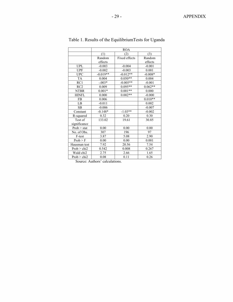
Following the existing literature, we estimated an equilibrium test of the following form:19 In( ROA it,) = α + β1 In UPLit + β2 In UPF it, + β3 In UPC it, +

γ1 In TA it + γ2 In RC1 it + γ3 In RC2 it+ γ4 DV + εi t

εi t = µi + νi t,

H = β1 + β2 + β3 = 0, where ROA is the pre-tax return on assets. As ROA can take on negative values on occasion, the dependent variable is computed as ln(1+ROA). The equilibrium test H = β1 + β2 + β3 = 0 tests whether the returns on assets are statistically significantly correlated with input prices, which in equilibrium they should not. The results of the equilibrium tests over the whole period as well as the sub-periods analyzed in this paper are presented in the table below, and a standard Wald-test is used to test the H=0 hypothesis. The results show that the market equilibrium condition cannot be rejected at the 5 percent level for the post-privatization period and the 10 percent level for the pre-privatization period but is close to being rejected at the 10 percent for the whole period. With the possible exception of the input price of fixed capital, input prices are thus not statistically different from zero and have not affected returns on assets in the two sub-periods. It makes intuitive sense that the banking system tended to move away from equilibrium during the privatization of UCB.20 Interestingly, returns on assets are positively associated with the loan ratio in both periods, while the nominal interest rate, inflation and the NPL ratio were important for profit in the pre-privatization period but not the in post-privatization period where foreign banks were associated with larger profitability.

19 See Molyneux et al. (1996) and Claessens and Laeven (2003) among others.

20 In fact, the equilibrium test for periods further away from the privatization period are more robust in accepting the null hypothesis of banking system equilibrium.

- 29 - APPENDIX

Table 1. Results of the EquilibriumTests for Uganda

ROA (1) (2) (3) Random

effects Fixed effects Random

effects UPL -0.003 -0.004 -0.001 UPF -0.002 -0.003 0.001 UPC -0.019** -0.012** -0.008* TA 0.004 0.050** 0.004

RC1 -.003* -0.005** -0.001 RC2 0.009 0.095** 0.062**

NTBR 0.001* 0.001** 0.000 HINFL 0.000 0.002** -0.000

FB 0.006 0.010** LB -0.011 0.002 SB -0.006 -0.007

Constant -0.148* -1.03** -0.002 R-squared 0.32 0.20 0.30

Test of significance

133.02 19.61 30.85

Prob > stat 0.00 0.00 0.00 No. of Obs. 307 196 97

F-test 3.87 5.08 2.90 Prob > F 0.00 0.00 0.001

Hausman test 7.92 20.56 7.54 Prob > chi2 0.542 0.008 0.267 Wald chi2 2.75 2.66 1.65

Prob > chi2 0.08 0.11 0.26 Source: Authors’ calculations.