Population Aging and the Real Interest

Rate in the Last and Next 50 Years

––A tale told by an Overlapping Generations Model––

Nao Sudo* nao.sudou@boj.or.jp

Yasutaka Takizuka* yasutaka.takizuka@boj.or.jp

No.18-E-1 January 2018

Bank of Japan 2-1-1 Nihonbashi-Hongokucho, Chuo-ku, Tokyo 103-0021, Japan

* Monetary Affairs Department

Papers in the Bank of Japan Working Paper Series are circulated in order to stimulate discussion and comments. Views expressed are those of authors and do not necessarily reflect those of the Bank. If you have any comment or question on the working paper series, please contact each author. When making a copy or reproduction of the content for commercial purposes, please contact the Public Relations Department (post.prd8@boj.or.jp) at the Bank in advance to request permission. When making a copy or reproduction, the source, Bank of Japan Working Paper Series, should explicitly be credited.

Bank of Japan Working Paper Series

1

POPULATION AGING AND THE REAL INTEREST RATE IN THE

LAST AND NEXT 50 YEARS*

--A tale told by an Overlapping Generations Model--

Nao Sudo† and Yasutaka Takizuka‡

January 2018

Abstract

Population aging, along with a secular decline in real interest rates, is an empirical regularity observed in developed countries over the last few decades. Under the premise that population aging will deepen further in coming years, some studies predict that real interest rates will continue to be depressed further to a level below zero. In the present paper, we address this issue and explore how changes in demographic structures have affected and will affect real interest rates, using an overlapping generations model calibrated to Japan's economy. We find that the demographic changes over the last 50 years reduced the real interest rate. About 270 out of the 640 basis points decline in real interest rates during this period was attributed to declining labor inputs and higher saving, which themselves stemmed from the lower fertility rate and increased life expectancy. As for the next 50 years, we find that demographic changes alone will not substantially increase or decrease the real interest rate from the current level. These changes reflect the fact that the size of demographic changes in years ahead will be minimal, but that downward pressure arising from the past demographic changes continue to bite in the years ahead. As Japan is not unique in terms of this broad picture of changes in demographic landscapes over the last 50 years and in the next 50 years, our results suggest that, sooner or later, a demography-induced decline in real interest rates may be contained in other developed countries as well. JEL classification: E20, J11 Keywords: Declining Real Interest Rates; Population Aging; Overlapping Generations

Model

* The authors are grateful to Hibiki Ichiue, Selahattin İmrohoroğlu, Jinill Kim, Takushi Kurozumi, Takashi Nagahata, Teppei Nagano, Kenji Nishizaki, Takemasa Oda, Masashi Saito, Tomohiro Sugo, Toshinao Yoshiba, and seminar participants at the Bank of Japan. The views expressed in this paper are those of the authors and do not necessarily reflect the official views of the Bank of Japan. † Monetary Affairs Department, Bank of Japan. E-mail: nao.sudou@boj.or.jp ‡ Monetary Affairs Department, Bank of Japan. E-mail: yasutaka.takizuka@boj.or.jp

1 Introduction

Over the last few decades, population aging and a secular decline in real interest rates

have gone hand-in-hand in major developed countries, though to varying degrees. Figure 1

shows the time path of real interest rates and �old-age�dependency ratios in G7 countries

over the last 50 years. Real interest rates have seen a continuing decline since the early

1980s, speci�cally since the end of the Great In�ation of the 1970s, and they have been

moving at a rate around zero in recent years. Meanwhile, population aging advanced

globally. Dependency ratios have continued to rise since the 1960s, and in some countries

the pace has even accelerated since the 1990s. In addition, according to the forecasts by

the U.N., or by other domestic authorities, the progress of population aging will continue

to deepen in the years ahead. Given the prospective changes in demographic landscapes,

some studies, such as Eggertson et al. (2017), point out the possibility that population

aging, combined with the e¤ects of other factors, could bring real interest rates down to a

value below zero for a prolonged period.

Questions about the in�uences of aging on macroeconomic variables have long attracted

the attention of scholars, including Auerbach and Kotliko¤ (1987) on the U.S. economy,

and Miles (1999) on the U.K. and European countries. What is di¤erent in recent years

is that central bank economists ventured into this area of research. Against the backdrop

of continuing low interest rates, there is a growing concern among central bankers that

the decline in real interest rates may be a signal that the natural rate of interest (or

equivalently, the long-run equilibrium real interest rate) �the real interest rate at which

economic activity and prices neither accelerate nor decelerate �is declining or will decline

in the years ahead, reducing the e¤ectiveness of monetary policy.1 ;2 While natural rates

of interest are not directly observable, there are suggestive estimates that support these

concerns. Figure 2 shows the time path of the natural rate of interest in selected countries

estimated based on the methodology developed by Laubach and Williams (2003). Clearly,

1The concern is clearly related to discussion about secular stagnation hypothesis. See, for example,Summers (2014, 2015) for the detailed discussion.

2Recent voices from central bankers regarding the relationship between population aging and real interestrates or the natural rate of interest include Carney (2017), Draghi (2016) and Fischer (2016).

2

some cross-country di¤erences notwithstanding, they all exhibit a declining trend and are

reaching around zero as of 2017.

In this paper, we address the relationship between population aging and real interest

rates by answering the following two questions: Have changes in demographic structures

so far a¤ected developments in real interest rates? And, will demographic changes lead

to a further decline in real interest rates in the years ahead? To this end, we construct

an overlapping generations (OG) model calibrated to Japan�s economy that consists of 80

generations of households, a social security system, and the government. Because we are

interested in analyzing the changes in the real interest rate that are induced by demographic

factors exclusively, our model abstracts from nominal rigidities and short-run structural

shocks, such as markup shocks or monetary policy shocks.3 We choose the OG model as it

is suited to precisely exploring the implications of changes in demographic landscapes for

factor prices, including the real interest rate, and allocations, isolating the e¤ects of other

factors, such as total factor productivity (TFP) or the tax and social security system.

We choose Japan�s economy, since, as illustrated in Figure 1, Japan is a country where

demographic changes are pronounced in terms of their pace and depth when compared

with other advanced countries. In the later section, however, we also quantify the e¤ects

of demographic changes on real interest rates in the other countries using data from these

countries.

With the model, we carry out perfect foresight simulations, similar to those conducted

in existing studies, such as Hayashi and Prescott (2002), Chen et al. (2007), Hansen and

·Imrohoro¼glu (2016), and Gagnon et al. (2016). We feed into the model the time paths

of exogenous variables, including demographic variables and TFP from 1960 onwards, and

compute the equilibrium transition paths of factor prices and allocations during that time.

We �rst show that our model explains the actual data well. That is, the model closely

3Along the same line, labor force participation rates are assumed to be constant over time in our model.Consequently, the dynamics of working-age population in the model does not coincide with those of thenumber of workers in Japan, period by period, because the latter mirror changes in labor force participationrates over the business cycles. It is also notable, however, that as suggested in Figure 6 below, when e¤ectsof changes in intensive margin are taken into account as well, the model-generated total labor inputs,namely the product of the extensive and intensive margin of the labor inputs, roughly agree with the datacounterparts, at least in terms of the long-run dynamics.

3

replicates the actual time path of GNP and other key variables from 1960 to 2015. We then

simulate the model under various di¤erent assumptions about demographic landscapes and

other exogenous variables, and study how changes in demographic factors are translated

to changes in the real interest rate.

Our answers to the two questions we address are Yes and No, respectively. On the

one hand, we �nd that changes in demographic landscape over the last 50 years, both the

decline in the fertility rate and the increase in longevity, have lowered the real interest

rate in Japan massively.4 A decline in the fertility rate directly reduces the working age

population and an increase in longevity encourages households� saving, leading to lower

labor inputs and higher capital accumulation, which in turn reduces real interest rates.

Based on our baseline simulation, 270 out of the 640 basis points decline in the real interest

rate from 1960 to 2015 was caused by the changes in the demographic structure. On the

other hand, the model also indicates that changes in the demographic landscape from 2016

onwards will have only a minor e¤ect on the real interest rate. Other things being equal, the

real interest rate will not increase or decrease much in response to the upcoming changes in

demographic factors, staying around the current level. Based on our baseline simulation,

the real interest rate will be evolving between 0 and 90 basis points over the next 50 years,

and the rates do not depart from that level much even when the demographic landscape is

arrested in that of 2015.

Why will the in�uence of demographic factors on real interest rates wane over the years,

and why is the real interest rate not going to decline further in the future? We argue that

there are two reasons. Most importantly, the magnitude of demographic change itself will

moderate over the course of history. In Japan, over the last 50 years, the fertility rate has

dropped from 4:6% in the 1960s to �0:7% in 2015, which results in a decline in the growth

rate of the working age population from 2:0% to �1:4% during the period. In the next 50

years, the fertility rate will drop by only 0:5%, which makes the growth rate of the working

age population almost unaltered. Similarly, life-expectancy has risen by 12 years over the

4To maintain consistency, we de�ne the �fertility rate� as the growth rate of the age-21 population.Admittedly, this de�nition is di¤erent from the common de�nition of the �total fertility rate,�which is theaverage number of children per woman during her lifetime.

4

last 50 years, but it will rise by only 4 years over the next 50 years. This �calming down�of

population aging suggests that the marginal increase of the downward pressure from now

on will be quantitatively minor. It is notable, however, that the e¤ects of the past changes

in demographic factors will continue to exert downward pressure on real interest rates. In

fact, the second reason is that the e¤ects of the past demographic changes are long-lived

and will not disappear in the years ahead, preventing the real interest rates from rising or

falling from current levels. This is partly because a rise in longevity is a permanent change

and a¤ects households�saving behavior permanently, bringing about a persistent negative

e¤ect on the real interest rate. Based on our baseline simulation, for example, the size of

the downward pressure on real interest rates due to changes in demographic factors during

the 1970s and 1980s is about 130 basis points as of 2015, and this will only shrink to about

90 basis points in 2060.

Lastly, we ask if our �ndings about the impacts of demographic factors on real interest

rates have global implications. Not surprisingly, declining the fertility rate and increasing

longevity and a moderation of these demographic changes over time are commonly observed

in developed countries. We therefore conduct similar simulation exercises again, this time

by feeding into our OG model the demographic variables of the U.S., G7 countries (less

Japan and U.S.), and 15 selected OECD countries (less Japan and U.S.). We compute the

in�uence of demographic factors on real interest rates in each of the country groups and

compare this with that for Japan. We show that, though some di¤erences are present across

these country groups, mirroring di¤erences in demographic developments, the negative

e¤ects of demographic factors on real interest rates and the waning in�uence of these

factors in the years ahead are also obtained for the country groups.

Our paper is based on the two strands of the literature. The �rst strand includes

analyses that explore the relationship between demographic structures and real interest

rates or the natural rate of interest, including Ikeda and Saito (2014), Fujita and Fujiwara

(2016), Rachel and Smith (2015), Gagnon et al. (2016), Carvalho et al. (2016), and

Eggertson et al. (2017). Our study is closest to the works by Gagnon et al. (2016) and

Eggertson et al. (2017) because they also use a medium-scale OG model as their analytical

5

tools. Similar to our work, Gagnon et al. (2016) document that the changes in demographic

structures, in particular those that took place before the 1980s, account for almost all of

the decline in real interest rates from 1980 to 2016 in the U.S., and that real interest rates

are likely to stay more or less at the current low level in the years ahead. Our paper is

also related to studies that explore the relationships between demographic structures and

macroeconomic variables, in particular those focusing on Japan�s economy using an OG

model. These studies include Chen et al. (2007), Braun et al. (2009), Braun and Joines

(2015), Muto, Oda, and Sudo (2016, MOS). In particular, our paper is close to MOS (2016)

in terms of its focus on population aging in Japan.5

The contribution of this paper is to quantify the impact of demographic factors, i.e.,

changes in the fertility rate and longevity, on real interest rates in the past and next 50

years, using an OG model calibrated to Japan�s economy and to examine the implications

for other developed countries, including the U.S. Clearly, our paper is not the �rst paper

to address this issue, but it di¤ers from existing studies in the following points. First, our

analysis is based on an OGmodel with heterogenous agents with age-speci�c characteristics,

and contrasts with other model-based approaches on the e¤ects of population aging on the

real interest rate in Japan, such as Ikeda and Saito (2014) and Fujita and Fujiwara (2016).

The use of an OG model allows us to provide a precise assessment of the distinct role

played by changes in the fertility rate and longevity that occur at di¤erent periods over

the course of history. Second, we show how the transmission of demographic factors to real

interest rates is a¤ected by other elements of economic environment. For example, while

existing studies with an OG model, including Gagnon et al. (2016) and Eggertsson et al.

(2017), disregard the tax system and the social security system, we show that the simulated

time path of the real interest rate is biased downward if the social security system is not

appropriately modeled. Third, we compare the impact of demographic changes across

5Our OG model is built upon the model of MOS (2016). The key departure from theirs is that webroaden our scope of the analysis in time-series dimension and study the 1960s onwards, instead of the1980s onwards as studied in MOS (2016). As we show below, changes in the demographic landscapes inthe 1960s and 1970s are substantially large, and, the e¤ects of these changes in�uence even today�s realinterest rates in an important manner. The current paper also di¤ers from MOS (2016) in its focus onthe dynamics of real interest rates, whereas MOS (2016) focus on the dynamics of other macroeconomicvariables, in particular, those of output growth.

6

countries and derive global implications about the role of population aging on the real

interest rates. This contrasts with existing studies that typically examine the implications

for a speci�c country or region.

The remainder of this paper is organized as follows. Section 2 describes an OG model.

Section 3 explains the calibration methodology and the data sources for simulation exer-

cises. Section 4 documents the simulation results under the baseline scenario for exogenous

variables including demographic factors. It shows how well the model replicates develop-

ments in macroeconomic variables from 1960 to 2015, and how the key variables will develop

over the next 50 years. Section 5 gauges the e¤ect of population aging on the real inter-

est rate by conducting simulations under hypothetical scenarios for demographic changes,

TFP, and the social security system. Section 6 draws global implications about the e¤ect

of population aging using a set of simulations equipped with demographic variables from

other developed countries. Section 7 concludes.

2 Model

Outline of our model

Our model is built up on a standard OGmodel, including that of Auerbach and Kotliko¤

(1987). Following MOS (2016), however, we incorporate two additional ingredients into

the otherwise standard model: (a) the health insurance system, and (b) a �bond-in-utility�

speci�cation developed in Hansen and ·Imrohoro¼glu (2016). We incorporate (a) because

the social security system is considered an important determinant of households�savings

behavior, and the ingredient (b) in order to address sizable and persistent positive spreads

between the real return on capital and the real interest rates on government bonds in the

actual data.6

2.1 Demographics

The time period of the model is discrete and annual. The economy consists of 80 generations

of di¤erent ages denoted by j = 21; :::; 100. In each period t, a new generation aged

6See Hansen and ·Imrohoro¼glu (2016) for the details of the rationale behind this setting.

7

21 is born into the economy, while the other existing generations all shift forward by

one. The oldest generation, j = 100, which we assume to be the maximum age, dies out

deterministically in the subsequent period. The growth rate of the new generation (age-21

households) in period t is denoted by �t; which we will hereafter refer to as the fertility

rate in the model. Then the age-21 population in period t, expressed as P21;t, is given by

P21;t = (1 + �t)P21;t�1: (1)

All households face a mortality risk that is common within the same cohort but may di¤er

across cohorts. They survive to the subsequent period with conditional survival probability

j;t, which is the probability that households aged j � 1 in period t� 1 survive to become

age j households in period t. Note that 101;t = 0 by assumption. Then the population,

Pj;t, and cohort share, �j;t, of age j households in period t are expressed as follows:

Pj;t = j;tPj�1;t�1; (2)

�j;t =Pj;tP100i=21 Pi;t

for j = 21; :::; 100: (3)

For the purpose of the ensuing analysis, we also de�ne the total population Pt as follows:

Pt �100Xi=21

Pi;t:

2.2 Households

Setting

Until mandatory retirement at age j = 65, households supply labor to �rms and earn

wage income according to their age-speci�c labor e¢ ciency denoted as "j;t from age j =

21 to 65, paying the labor income tax and payroll income taxes that cover social security

bene�ts in every period.7 Households aged j = 66 withdraw from the labor force, and those

7Although mandatory retirement in Japanese �rms is usually set between age 60 and 65, labor forceparticipation rates above age 65 are never zero according to data, though they are not sizable. Followingexisting studies such as Chen et al. (2007) and MOS (2016), however, we maintain the conventionalassumption because detailed and su¢ cient data on wages, hours, and the number of workers above age 65

8

aged j � 66 receive public pension bene�ts from the social security system. Throughout

their lives, households save assets in two forms, capital and government bonds, and receive

capital income arising from these assets.

In every period T , newly born households choose sequences of consumption, labor,

capital and bond holdings in t � T , to maximize their expected lifetime utility (discounted

by the subjective discount factor �)

100Xj=21

�j�21

"jY

i=21

i;T�21+i

#u (cj;t; hj;t; bj+1;t+1) (4)

subject to the budget constraints over their lifetime

(1 + � c;t) cj;t + kj+1;t+1 + bj+1;t+1 + �j;tmbj;t

=�1 + (1� �k;t) rKt

�kj;t + (1 + r

Bt )bj;t (5)

+ (1� �h;t) (1� � s;t � �m;t)wt"j;thj;t + � t + �t for j � 65;

(1 + � c;t) cj;t + kj+1;t+1 + bj+1;t+1 + �j;tmbj;t

=�1 + (1� �k;t) rKt

�kj;t + (1 + r

Bt )bj;t + pbj;t + � t + �t for j > 65: (6)

Note that in a period t � T; these households are at the age of j = t � T + 21. cj;t is

consumption and hj;t is labor supply. kj;t and bj;t denote capital and bond holdings of age

j households at the beginning of period t. wt is the wage rate, rKt is the before-tax real

rate of return on private capital, and rBt is the after-tax real rate of return on government

bonds. � c;t is the consumption tax rate, �h;t and �k;t are the tax rates on income from

labor and capital, and � t is a lump-sum transfer in period t.8 �t is a lump-sum transfer

associated with accidental bequests, which are left by households who die in the preceding

period t� 1. � s;t and �m;t are the payroll income tax rates (contribution rates) for public

pension and health insurance, respectively. "j;t is age-speci�c labor e¢ ciency for j � 65;

is not available.8This corresponds conceptually to what is categorized as the sum of the net current transfers and the

capital transfers in the System of National Accounts in Japan.

9

pbj;t is public pension bene�ts that retirees aged j in period t receive, described later. The

age-speci�c pro�le of medical costs, denoted by mbj;t, is assumed to be exogenously given.

As shown in the equations above, only a proportion of the medical expenditures is paid

directly by each household. We denote this copay rate by �j;t 2 [0; 1]. We assume that

this rate di¤ers across ages and time so that they are consistent with the past and present

institutional structure.9 We assume that a new household born in period t has no initial

assets: k21;t = b21;t = 0.10 While no household is able to survive to the maximum age

100, it doesn�t fully consume its assets at the age of 100 because of a bequest motive:

k101;t > 0 and b101;t > 0. We also assume that the government collects all accidental

bequests including capital income in period t�1, and redistributes them equally among all

households alive in period t. The total amount of accidental bequests in period t is given

by

�t =101Xj=22

(1� j�1;t�1)��1 + (1� �k;t�1) rKt�1

kj�1;t�1 + (1 + r

Bt�1)bj�1;t�1

� Pj�1;t�1Pt

: (7)

Following Hansen and ·Imrohoro¼glu (2016), we introduce government bond holdings

into the utility function. The basic idea behind this �bond-in-utility� speci�cation is to

incorporate households�preference for the liquidity and safety characteristic of government

bonds. The functional form of households�utility is assumed to be separable in terms of

its arguments, which are given as

u (cj;t; hj;t; bj+1;t+1) = log cj;t � th1+ 1

�j;t

1 + 1�

+ �t log(bj+1;t+1 + b) for j � 65; (8)

u (cj;t; hj;t; bj+1;t+1) = log cj;t + �t log(bj+1;t+1 + b) for 65 < j < 100;

u (cj;t; hj;t; bj+1;t+1) = log cj;t + �(log bj+1;t+1 + log kj+1;t+1) for j = 100;

where b is the parameter that limits the curvature of the period utility function when

9The copay rate is 30% for people below 70 and virtually 0% for people over 69 until 2002. The copayrate is approximately 10% for people over 69 from 2003 to 2007. After 2007, the rate is approximately 20%for people of age 70 to 74 and 10% for people over 74.10The borrowing constraint is not imposed on households�assets in our model. In other words, households

are allowed to borrow against their future income.

10

bj+1;t+1 is close to 0, and � is the Frisch elasticity of households�labor input supply. t

and �j;t are the time-varying parameters households�preferences for leisure and government

bond holding in period t. Higher t or �t implies that households put a higher value on

leisure or government bond holding. For households aged 100, we assume that they have

the bequest motive, following Eggertsson et al. (2017) and Lisack et al. (2017). Note that

� is the parameter that determines the relative importance of the bequest motive.

Since households receive utility from government bond holding (i.e., �t > 0), the �rst

order conditions of age j households in period t yield the following equation regarding the

spread �t of the two asset returns:

�t � (1� �k;t)rKt � rBt =1

�(1 + � c;t)�t

100�1Xj=21

�j;tcj;t

(bj+1;t+1 + b): (9)

The above equation shows that the spread �t is wide when the preference parameter �t

is high or the size of government bond holding relative to the consumption is low. This

re�ects the fact that households are willing to hold low-return assets only if the marginal

utility from holding them is greater.

2.3 Firm

There is a representative �rm producing �nal goods with the Cobb-Douglas production

technology. In perfectly competitive spot-markets the �rm rents capital and hires labor

from households so as to maximize its pro�t

�t = AtK�t L

1��t �RtKt � wtLt; (10)

where � is the capital share of output, Kt is aggregate capital stock, Lt is aggregate labor

input, and Rt is the rental rate of capital stock. At denotes TFP, and we assume that the

TFP factor grows at the rate of gt in every period:

gt � (At=At�1)1=(1��): (11)

Note also that the output, or equivalently GNP, in the economy coincides with the size

11

of the aggregate product. That is,

Yt = AtK�t L

1��t :

In equilibrium, the factor prices are given by

Rt = �At

�Kt

Lt

���1� rKt + �t; (12)

wt = (1� �)At�Kt

Lt

��; (13)

where �t is the depreciation rate of capital stock. The aggregate demand for capital and

labor inputs is equalized to the aggregate supply of these primary inputs, so as to clear the

respective markets in every period:

Kt =

100Xj=22

Pj�1;t�1kj;t; (14)

Lt =65Xj=21

Pj;t"j;thj;t: (15)

Here, the evolution of the aggregate capital stock is given by

Kt+1 = It + (1� �t)Kt: (16)

where It is aggregate investment. Relatedly, the aggregate saving rate st is de�ned by the

following equation.

st �It � �tKt

Yt: (17)

2.4 Social Security System

The social security system is divided into two sections: public pension and health insurance.

The public pension bene�t pbj;t provided to age j households in period t depends on their

historical wage income, being proportional to the average wage income that households

have received during their working years, following Chen et al. (2007). The public pension

12

bene�t provided by the social security system to a new retiree in period t is given as

pb65+1;t ��t

65 + 1� 21

65Xi=21

fwt+i�65�1"j;thi;t+i�65�165+1�iYk=1

gt+i+k�65�1g: (18)

The public pension bene�t that age j households receive is formulated as

pbj;t = 0 for j = 21; 22; :::; 65;

pbj;t =�t

�t+65+1�jpb65+1;t+65+1�j ; for j = 65 + 1; :::; 100: (19)

�t is the replacement ratio that determines the size of the public pension bene�t relative

to the past wage. The pension bene�t paid to households in the same cohort is constant

throughout their lifetime as long as the replacement ratio is unchanged. Note, however,

that compared to the cohort a generation before, the next generation receives a di¤erent

size of bene�ts depending on the growth rate of TFP.

For both public pension bene�ts and medical bene�ts, part of the costs is covered by

the government, and the rest is covered by the relevant section of the social security system.

Taking as given the coverage ratios of transfers/expenditures �nanced by the government,

which we denote as �s;t and �m;t, the social security system adjusts the contribution rates

for public pension and health insurance, � s;t and �m;t, in every period in the following

manner:

� s;t =(1� �s;t)

P100j=65+1 Pj;tpbj;t

wtP65j=21 Pj;t"j;thj;t

; (20)

�m;t =(1� �m;t)

P100j=21 Pj;t (1� �j;t)mbj;t

wtP65j=21 Pj;t"j;thj;t

: (21)

2.5 Government

The government raises revenues by newly issuing one-period government bonds and levying

taxes on households�consumption, labor income, and capital income, to �nance its spending

that is the sum of government purchases, transfers/expenditures to the social security

system, interest repayments on government bonds, and other lump-sum transfers. Taking

the sequences of government revenues and spending as given, government bond issuance is

13

adjusted so that the following consolidated budget constraint holds in every period:

(1 + rBt )Bt +Gt + �m;t

100Xj=21

Pj;t (1� �j;t)mbj;t + �s;t100X

j=65+1

Pj;tpbj;t +100Xj=21

Pj;t� t

= Bt+1 + � c;tCt + �h;t(1� � s;t � �m;t)wtLt + �k;trKt Kt; (22)

where Gt and Bt are government purchases and government bonds at the beginning of

period t, respectively. Note that the supply of government bonds is equalized to the sum

of households�bond holdings in each period:

Bt =100Xj=22

Pj�1;t�1bj;t: (23)

2.6 Real Interest Rates in the Model

In this model, households can hold two types of assets, capital stock kj;t and government

bonds bj;t, and there are two di¤erent asset returns rKt and rBt . Because of the bond-in-

utility setting, the return on capital rKt is generally higher than the return on government

bonds rBt .11 Throughout this paper, we refer the latter as the real interest rate, and

study the e¤ects of changes in demographics on this rate. We do so for the purpose of

comparison with existing studies on the natural rate of interest, including Laubach and

Williams (2003), Gagnon et al. (2016), Fujiwara et al. (2016) and Eggertsson et al. (2017).

While spreads between the return on capital and the risk-free rate are universally observed

and not unique to Japan, the natural rate of interest in these studies is either estimated

using the data of the risk-free rates, such as the call rate or the government bond yield,

or analyzed under the premise that the return on capital and the return on government

bonds are equalized ex-ante to the level of prevailing risk-free rates.12

11 In fact, the spread between the two assets measured by the System of National Accounts has been sizablein Japan. For example, as of 2015, the after-tax return on capital, measured as the operation surplus dividedby the total capital stock is 6.8% whereas the after-tax return on government bonds, measured as the netinterest payment by the government divided by government bonds outstanding, is 0.1%.12While the returns on capital rKt and the return on government bonds rBt are sizably di¤erent in level,

as we show below, the di¤erence is negligible when comparing the e¤ect of demographic changes on thetwo rates. This is because, in our simulation setting, thanks to the assumption regarding the government�stransfer rule described below, the spread between the two returns �t is barely a¤ected, if at all, by changesin demographic factors.

14

3 Data, Calibration, and Assumptions

In our simulation, we compute the equilibrium transition paths of allocations and prices,

including real interest rates, from given initial conditions in 1960 toward a steady-state far

in the future, taking the sequence of exogenous variables from 1960 to the far future. We

feed three classes of inputs into the model: (i) structural parameters such as those of the

production function, (ii) exogenous variables such as fertility rates and tax rates, and (iii)

the steady state distribution of households�assets. In this section, we describe in detail

how to construct these inputs and how to compute the equilibrium path.

3.1 Structural Parameters

The structural parameters of our model, �; �; and � are calibrated based on information

from the sample period running from 1960 to 2015 and their values are listed in Table 1.

The capital share of the production function � is 0:362 which is the same value as Hayashi

and Prescott (2002). The subjective discount factor � is set so that our benchmark model

replicates well the time path of the capital-output ratio during the sample period, and the

value of Frisch elasticity � is set at 0:5 so that our benchmark model captures an average

life-cycle pattern of labor inputs during the same period. In addition, the parameter that

limits the curvature of the period utility function b is set to 0:11; following Hansen and

·Imrohoro¼glu (2016), and the parameter for relative importance of the bequest motive � is

set at 18.33, so that it is consitent with the equilibirum condition for households with age

100:13

3.2 Exogenous Variables

We conduct perfect foresight simulations from 1960 to 2015 and beyond, by feeding into

the model the time paths of exogenous variables from 1960 to in�nity and computing the

equilibrium prices and allocations. There are four classes of variables; those related to

demographics, to production technology, to households, and to the government. Some of

13 In calibrating the value for �; we use the age-speci�c expenditure and savings documented in NationalSurvey of Family Income and Expenditure for 2014 and obtain the data for c100;t and k101;t by interpolation,and choose � that meets the �rst order condition of these households.

15

the exogenous variables are age-speci�c, shown in Figure 3, and other exogenous variables

are shown in Figure 4.

Production technology: Exogenous variables regarding production technology in-

clude the depreciation rate of capital stock f�tg1t=1960, and the growth rate of TFP fg1��t g1t=1960:

For t � 2015, We use the actual data from 1960 to 2015. For t � 2016, we use the actual

value as of 2015 for the depreciation rate �t and the average of actual values from 2010 to

2015 for the growth rate of TFP g1��t ; 6:2% and 1:1%, respectively. Note that the latter

value is close to the 1% �gure estimated by the Cabinet O¢ ce (2017) as the TFP growth

rate in the early 2020s.

Households: Exogenous variables regarding households include the preferences for

leisure f tg1t=1960, these for bond holding f�tg1t=1960; age-speci�c medical expenditures

ffmbj;tg100j=21g1t=1960, and labor e¢ ciency ff"j;tg100j=21g1t=1960. The �rst variable t is constant

from 1960 until the late 1980s. After 1989, it gradually increases over a couple of years,

and stays at the constant in the subsequent years.14 The second variable �t is set so that

the spread �t generated from the baseline simulation coincides with the data counterpart

for t � 2015:15 We use the actual data, taken from Estimates of National Medical Care, for

the medical expenditures fmbj;tg100j=21 for 1980 � t � 2015: For t � 1979, we calibrate the

values with the aggregate �gures of the same estimate, using the distribution of ages as of

1980, fmbj;1980g100j=21: As shown in Figure 3, the medical costs monotonically increase with

age. It is also notable that the e¤ects of aging on the costs are more pronounced in recent

years. In addition, we use actual data for the age-speci�c labor e¢ ciency f"j;tg100j=21 for

1988 � t � 2015, following the method of Braun et al. (2009). For t � 1987, we calibrate

the values to f"j;1988g100j=21. For t � 2016, we use the value as of 2015 for the preferences for

leisure t and for bond holding �t; and age-speci�c labor e¢ ciency f"j;tg100j=21. Furthermore,

14We intend to capture the gradual reduction in the statutory workweek stipulated in the Labor StandardsLaw revised in 1988. This reduction started in 1989 and ended in 1994.15The data counterpart is constructed from SNA for 1980 � t � 2015, and by interpolating the real

interest rate series constructed following Kamada (2009), for t � 1979:

16

in t � 2016, we assume that fmbj;tg100j=21 grows at the rate of TFP gt:

Government: Exogenous variables regarding the government include tax rates f� c;t;

�h;t; �k;tg1t=1960; government expenditures fGt=Ytg1t=1960; government transfers to house-

holds f� t=Ytg1t=1960; and government transfers to the social security system f�s;t; �m;t;

�t; f�j;tg100j=21g1t=1960: We use the actual data from 1960 to 2015 for those variables. For

t � 2016, we use the value as of 2015 for the tax rates other than the consumption tax

rate � c;t. The consumption tax rate � c;t is assumed to increase to 10% in 2019 and remain

unchanged from that rate in the subsequent years.

We assume that the government makes transfers to households in addition to � t in

period t � 2016 such that the government debt-to-GNP ratio fBt=Ytg1t=2016 is set so that

the model-generated value of the spread �2016 is unchanged in the following years. Under

this transfer rule is set so that the projected real interest rate rBt is not a¤ected by the

spread term �t in 2016 onwards, and variations of the real interest rate come from those

of the return on capital rKt exclusively during this period.16 ;17

Population: Exogenous variables regarding population include the growth rate of the

age-21 population (i.e., the �fertility rate� in our model) f�tg1t=1960, and the conditional

survival probability ff j;tg100j=21g1t=1960. We use the actual data from 1960 to 2015. For

t � 2016, we use as the benchmark the medium-fertility and medium-mortality variants of

population forecasts calculated by the National Institute of Population and Social Security

16Note that as shown in equations (9) and (23), the spread �t decreases with the amount of governmentbonds outstanding Bt: When the government issues more bonds to �nance its increasing expenditures andtransfers due to aging, therefore, the larger government bond causes a decline in the spread and a risein the real interest rate rBt , keeping the real return on capital stock r

Kt constant. Our assumption about

the government�s transfer rule described here aims to isolate this channel from our analysis. The mainreason we choose this approach is because, as shown in panel (10) of Figure 4, the parameter value of�t has varied substantially from 1960 to recent years. This indicates that, based on our model, a largeportion of variations in the spread �t has been driven by changes in �t rather than the endogenous e¤ectsof government bonds and consumption shown in equation (9) :17Similar to ours, related studies on Japan�s economy also assume some form of government debt policy in

order to ensure the transversality condition of the government over a long horizon. Hansen and ·Imrohoro¼glu(2016) assume that the government follows the trigger rule that raises tax rates when the government debt-to-GNP ratio exceeds a predetermined level. MOS (2016) assume a regime switch of government debt policythat will take place in 2050. In the model, from 2050 and beyond, the government adjusts the lump-sumtax so as to maintain the government bond-to-GNP ratio at its target level.

17

Research (IPSS). In addition, we use the high and low variants of population forecasts of

the IPSS and the �gures calculated by the UN for the purpose of the robustness check.

Demographic landscape in Japan

It is useful to sketch here the outline of changes in the demographic landscape over

time in Japan. The top two panels in Figure 5 show the time path of life expectancy and

the growth rate of the working age population. As shown in Figure 3, the conditional

survival probabilities f j;tg100j=21 have increased monotonically and permanently since 1960

at almost all ages. The life expectancy has risen accordingly from 71 in 1960 to 84 in

2015. Based on the projections of both by the IPSS and the UN, this upward trend will

continue in the years ahead, but at a moderate pace, reaching age 88 in 2060. The working

age population exhibits a secular decline from the 2000s and continues shrinking in the

subsequent years. It has grown on average at an annual rate of 0:5% over the last 50 years,

re�ecting the high fertility rate during the period, as shown in Figure 4. The growth rate

fell to below zero in the late 1990s, and will fall further to an annual rate of �1:1% over

the next 50 years. The entry and exit of baby boomers has a signi�cant impact on the

working population growth rate. The bumps in the early 1970s and the mid-1990s were

the result of the entries of the �rst and second baby boomers, respectively, and the hollows

in the early 2010s and 2040s will a consequence of their exits from the labor market.18

The bottom panel shows the distribution of the population by the age of for four

di¤erent periods: 1960, 1980, 2015, and 2040. The distribution changes shape drastically

over time. In the early days, the peak of the distribution was around the age of 20s to 30s,

and fewer people appeared above 30s. In addition, the density declines as the ages become

higher. In the present day, the distribution has two modes; one peak located around 40s,

and the other around the late 60s. In 2040, the distribution has only one mode, located

around the late 60s. It is also notable that while the general shape of the distribution in

the present day mostly coincides with that in 2040, the shape di¤ers markedly from that

18We de�ne the �rst and second baby boomers as those who were born in 1947�1949 and 1971�1974,respectively, following the convention.

18

in the early periods. This observation suggests that demographic changes that have taken

place so far are quantitatively larger than those that will take place in the years ahead.

3.3 Simulation Procedures

In all of the ensuing simulations, we assume perfect foresight. That is, newly-born house-

holds in period t are informed of the sequence of exogenous variables shown in Figures

3 and 4 from t onwards, and optimally determine their life-time consumption and labor

supply.

We compute the endogenous variables, namely prices and allocation in the economy, by

the shooting algorithm used in existing studies, such as Hayashi and Prescott (2002), Chen

et al. (2007), and Hansen and ·Imrohoro¼glu (2016). Given the two steady states, the initial

steady state including the initial asset distribution fbj;1960g100j=21 and fkj;1960g100j=21;19 and

the ending steady state to which the economy ultimately converges in the in�nite future,

we extract the sequence of prices and allocation in the economy from 1960 to the in�nite

future, that satis�es the equilibrium conditions under the given sequence of the exogenous

variables. The calibrated ending steady state values of key variables are presented in Table

2.

4 Baseline Simulations

The baseline simulation is conducted by feeding into the model the set of exogenous vari-

ables whose values are set as described above, and computing the endogenous paths of

prices and allocations.

19We do not have a detailed data set on the asset distribution for 1960, which is the initial year in ourmodel. To obtain the initial distribution of assets in 1960, kj;1960 and bj;1960, we �rst consider the steadystate of an economy where the exogenous variables are constant and their values are calibrated to theactual values of 1960, and compute the life-cycle pro�les of capital stock holdings kj and government bondholdings bj in this hypothetical economy. We then multiply the age-speci�c capital holdings kj at all agesby the same scalar qk so that the aggregate capital stock-to-output ratio K1960=Y1960 computed from themodel coincides with the actual data: kj;1960 = qk� kj . We do the same to the age-speci�c governmentbond holdings bj so that the aggregate government bond outstanding-to-output ratio B1960=Y1960 is thesame between the model and the data: bj;1960 = qb� bj .

19

4.1 Model�s Prediction on Households�Life-cycle Properties

Before analyzing the model�s dynamics, here we assess our model�s prediction about house-

holds�life-cycle pro�les with the data. Figure 6 shows the life-cycle pro�les of labor supply

hj , and the capital stock holdings kj for j = 21; :::100 generated by our model and in the

data.20 Our model replicates well the general pattern of life-cycle pro�les of these variables.

Labor supply increases gradually and moderately as households age from 21 to around 50s

and starts to decline at a quick pace from the peak to the level close to zero at ages above

50. The gap between the data and the model at ages around 70 re�ects the fact that in the

data there are households who work after the mandatory retiring age of 65. Capital stock

holdings also increase from the age of 21 until the age of around 60s in both the model and

the data. In the model, households start to deccumulate capital stock after the retirement

age. In the data, by contrast, the capital stock holdings continue to increase, though at a

slower pace than earlier ages, possibly due to the presence of the retirement allowance.

4.2 Model�s In-sample Performance

We �rst assess the �in-sample performance� of the model by comparing the endogenous

paths of prices and allocation from 1960 to 2015 that are generated from the model with

those of the data counterparts. Figure 7 shows the time paths of the key variables of the

economy; after-tax real return on capital (1� �k;t) rKt , the saving rate st, GNP per capita

(de�ned as real GNP divided by total population) Yt=Pt, the GNP growth rate Yt=Yt�1,

the capital-labor ratio Kt=Lt, the capital share of total assets Kt= (Kt +Bt), the pension

bene�ts-to-GNP ratio, the medical bene�ts-to-GNP ratio, and the primary balance-to-

GNP ratio. The dashed red lines show the actual data series, and the solid blue lines show

the model-generated series.

In summary, our model successfully replicates the actual dynamics of the key macro-

20For the data, the life-cycle pro�les of capital stock holdings kj are based on the National Survey ofFamily Income and Expenditure. Note that because there is no detailed data available for a life-cycle pro�leof government bond holdings bj , we assume that households at all ages hold government bonds relative tototal assets aj by the same proportion as the aggregate government bond outstanding-to-aggregate totalasset ratio. A life-cycle pro�le of labor supply hj is constructed from a life-cycle pro�le of working hoursbased on the Basic Survey on Wage Structure, and the life-cycle pro�les of the labor participation rateand labor force based on the Labor Force Survey.

20

economic variables over the sample period. For example, similar to the data, our model

generates the �Golden Sixties�or �Japan�s miracle,�the rapid GNP growth rate seen dur-

ing the 1960s, and also generates the �Lost decade(s),� the sudden and persistent GNP

slowdown starting from the early 1990s. The model also yields the secular decline in return

on capital, including its drastic fall in the mid-1970s, which is seen in the actual data. The

long-run developments of revenues and expenditures of the social security system and the

government, such as the persistent increases in pension and medical bene�ts, the deteri-

oration in the primary balance of the government, and the accelerating government debt

accumulation, are all replicated in the model.

For the real interest rate rBt , we compare the time path of the model-generated �gure

with a set of the natural rate of interest estimated in existing studies.21 Figure 8 shows

the time path of the model-generated series of the real interest rate rBt and the after-tax

return on capital (1� �k;t) rKt ; and two measures of the natural rate of interest in Japan�s

economy that are estimated based on the methodology of Laubach and Williams (2003) and

Imakubo et al. (2015), and the potential growth rate constructed by the Bank of Japan.22

While the comparison is only possible from the 1980s onwards, the model-generated real

interest rate rBt closely tracks the secular decline that commonly appears in these measures,

and captures the low level of the rate in recent years.

4.3 Out-of-sample Simulation

Figure 9 shows out-of-sample projections for the real interest rate and GNP from 2016

onwards under the baseline scenario. Roughly speaking, the real interest rate rBt will stay

at the 2015 level in the years ahead, mirroring the fact that the return on capital rKt will

stay at the current level. Precisely speaking, however, based on the projections of both

the IPSS and the UN, both rates will continue gradually and modestly declining until mid-

21Here, we do not compare the model-generated real interest rate rBt with the data counterpart. Thisis because for the period from 1960 to 2015 we calibrate the households� preferences on bond holdingsf�tg

2015t=1960 so that the model-generated real interest rate r

Bt captures the movements of the data counterpart,

namely the government bond yield based on the SNA.22As discussed in Fujiwara et al. (2016), based on a standard representative agent model, the natural

rate of interest coincides with the potential growth rates on a per capita basis, at the steady state, undercertain conditions.

21

2040, when they will reach their nadir, which is about 20 basis points for the real interest

rate rBt and 450 basis points for the return on capital rKt , before ascending gradually in

subsequent years.

Japan�s GNP Yt will grow at the rate of about 1% growth for the next ten years,

gradually deccelerating to a rate around 0%. From 2040 and beyond, GNP grows at a

nearly zero rate. As shown in panel (3) where the growth rate of GNP is decomposed into

contributions of TFP At, labor inputs Lt, and capital inputs Kt, TFP growth, At=At�1; of

1:1% is almost exactly o¤set by declines in the growth rate of labor inputs Lt. Although

GNP growth declines to a rate around zero in the long run, as shown in panel (4), GNP

per capita Yt=Pt maintains above 1% growth in years ahead. This is primarily because, on

a per capita basis, declines in the growth rate of labor inputs Lt are relatively moderate,

while capital inputs Kt grow at a positive rate, boosting the growth rate of the output Yt.

5 E¤ects of Demographic Changes on Real Interest Rates

How much have demographic changes in�uenced real interest rates rBt so far, and how

important will they be in the years ahead? This section answers these two questions with

the help of four di¤erent types of simulations listed below.

1. Simulations under hypothetical assumptions about demographic structures, f�tg1t=1960and ff j;tg100j=21g1t=1960; where developments in demographic structures are perma-

nently arrested after the end of a speci�c decade, such as the 1960s, and, in the

subsequent years, remain unchanged at the average values in those ten years,

2. Simulations under hypothetical assumptions about demographic structures, f�tg1t=1960or ff j;tg100j=21g1t=1960; where developments in either the fertility rate and longevity

are arrested after the end of a speci�c decade and, in the subsequent years, remain

unchanged at the average values in those ten years,

3. Simulations under hypothetical assumptions about TFP growth rates fAt=At�1g1t=1960;

4. Simulations based on an alternative model economy where the social security system

22

is absent

The type 1 simulations intend to identify the timing of demographic changes that are

essential in shaping the long-run picture of real interest rate dynamics. In particular, we

are interested in comparing the e¤ect on the real interest rate of demographic changes that

have taken place over the last 50 years with those that will take place in the next 50 years.

The type 2 simulations intend to separately assess the consequences of falling fertility rate

and those of increasing longevity, and to determine the key transmission channel within

demographic factors. The type 3 and 4 simulations serve as the robustness analysis. We

intend to see if what we obtain from the type 1 and 2 simulations regarding the role

of demographic factors can fundamentally change when economic environments are also

di¤erent.

5.1 Interest Rates When Developments of Demographic Structure Ar-

rested

Figure 10 shows the results of the type 1 simulations. In the �gure, �Fixed in the Xs�

indicates that the fertility rate �t and the conditional survival probabilities f j;tg100j=21 both

take the values assumed under the baseline simulation up to the end of the Xs and, in

the subsequent years, take the average values of the previous ten years.23 The average

life-expectancy and the working-age population growth under the alternative assumptions

are documented in Table 3.24

The top panel shows the time path of the real interest rate rBt computed under various

assumptions about the timing when demographic changes are arrested. The middle and

bottom panels show the real interest rate rBt , labor inputs Lt, and capital inputs Kt,

in terms of the discrepancy between the variables computed under each of the alternative

assumptions about the timing, and those computed under the baseline assumption, namely

those shown in Figure 9.

23The only exception is the simulation named �Fixed in 2015.� In this case, the fertility rate �t and theconditional survival probabilities f j;tg100j=21 are the actual values up to 2015 and, in the subsequent years,are held constant as of 2015.24Because we hold the fertility rate �t constant but do not hold the working age population growth rate

constant, the latter series continues to vary in years after the year X:

23

Two observations are notable. First, demographic changes have so far depressed the

real interest rate rBt and will depress the rate in the years ahead. This is seen in the positive

gap between the real interest rate generated from the four hypothetical simulations and

those generated from the baseline simulation. For example, as of 2015, the real interest

rate rBt of �Fixed in the 1960s� is 270 basis points higher than the rate computed under

the baseline assumption. This gap stands for the quantitative impact on the real interest

rate rBt of demographic changes from the 1970s and beyond: The sign of this gap is positive

across all of the alternative simulations.

Second, the e¤ect on the real interest rate rBt of demographic changes that have already

occurred is larger than the e¤ect of those that is going to occur in the future. This is seen by

comparing the discrepancy series shown in panel (2). For example, the di¤erence between

the series of �Fixed in the 1960s�and of �Fixed in 2015�captures the e¤ects of demographic

changes from the 1970s to 2015, and the series of �Fixed in 2015� captures the e¤ect of

demographic changes in 2016 and beyond. As of 2015, the former e¤ect is about �260

basis points while the latter is about �10 basis points. Even in 2050, while the former is

about �220 basis points, the latter is about �70 basis points. Relatedly, it is also notable

that the e¤ect of the demographic changes are both persistent and sizable. Using the same

numerical example, the e¤ect of demographic changes from the 1970s to 2015 diminishes

only by 80 basis points from 2015 to 2060.

Why do demographic changes reduce the real interest rate rBt ; and why is the e¤ect

of those in the past larger than those in the future? In the current model, the dynamics

of the real interest rate rBt are almost entirely determined by what happens to the return

on capital rKt ; and the latter series is determined by the scarcity of the aggregate capital

inputs Kt relative to the aggregate labor inputs Lt; based on the aggregate production

function (10).25 How are then aggregate capital inputs Kt and labor inputs Lt driven

by demographic factors? As shown in panels (3) and (4), demographic factors drive the

production inputs into opposite directions under the most of the simulations. Namely,

25This is because the real interest rate rBt in the model is formulated as the return on capital rKt minusthe spread �t; and the size of the spread �t is held constant by the government policy in 2016 and beyondas assumed in Section 3.2.

24

labor inputs Lt increase and capital inputs Kt decrease when demographic developments

are arrested at a speci�c period.26 Given the form of the aggregate production (10), such

developments in production inputs lead to a lower real interest rate rBt ; re�ecting the

relative scarcity of labor inputs Lt.

It is also seen that the e¤ects on production inputs Kt and Lt of demographic changes

in the past are larger than those of demographic changes in the future. For example, in

panel (3) and (4), the di¤erence between �Fixed in the 1960s� and �Fixed in 2015� and

the series of �Fixed in 2015� indicate that, in terms of the magnitude, the impact on

production inputs of demographic changes that took place over the last 50 years is larger

than that of changes that will occur in the next 50 years.

5.2 Decomposing E¤ects of Fertility Rates and Longevity

Now we study in detail how each of the two components of demographic factors, the fertility

rate �t and the conditional survival probabilities f j;tg100j=21 a¤ects the real interest rate rBt ,

based on the type 2 simulations. To this end, we �rst conduct the following four simulations

that di¤er from each other in terms of assumptions about exogenous variables fed into the

model: (i) baseline simulation, (ii) baseline simulation except that the fertility rate �t in

the 1970s and beyond is set at the average value of the 1960s,27 (iii) baseline simulation

except that the survival probability rates f j;tg100j=21 from the 1970s and beyond are set at

the average values of the 1960s,28 and (iv) baseline setting except that both the fertility rate

�t and the survival probability rates f j;tg100j=21 from the 1970s and beyond are set to the

average values of the 1960s. We then de�ne the measure of �impact of longevity,��impact

of fertility rates,�and �impact of demographic factors,�of a variable Xt as follows.29

26 In the case of �Fixed in the 2000s,� labor inputs Lt increase instead of decrease, compared with thebaseline. This re�ects the fact that the fertility rate �t during the 2000s was on average about 1% lowerthan the rate in subsequent years starting in 2016 and ending in 2060.27Similar to the simulations above, this speci�cation indicates that f�tg

1t=1970 = 10

�1P9s=0 �1960+s.

28Again, similar to the simulations above, this speci�cation indicates that�f j;tg100j=21

1t=1970

=

10�1P9

s=0f j;1960+sg100j=21.

29Notice that the sum of the �impact of longevity�and �impact of fertility rates� should quantitativelycoincide with �impact of demographic factors.�However, because our simulations are based on the shootingalgorithm and therefore can capture e¤ects arising from the cross-terms of the fertility rate and longevity,these two �gures do not coincide exactly, though the di¤erence is quantitatively minor.

25

� Impact of longevity � fXt under simulation (ii)g � fXt under simulation (i)g ;

� Impact of fertility rates � fXt under simulation (iii)g�fXt under simulation (i)g ;

� Impact of demographic factors� fXt under simulation (iv)g�fXt under simulation (i)g :

Figure 11 shows the time paths of impact of fertility rates �t, that of longevity f j;tg100j=21,

and impact of demographic factors for the real interest rate rBt ; the growth rate of GNP

Yt; production inputs Lt and Kt on a per capita basis, and the saving rate st. Except for a

few years in the early 1960 or 1970s, in all of the simulation periods, demographic factors

depress the real interest rate rBt , both through the declining fertility rate and increasing

longevity. In addition, the two impact series are quantitatively comparable. As of 2015,

for example, half of the decline in the real interest rate rBt was attributed to changes in

the fertility rate, and the other half was attributed to changes in longevity.

Transmission mechanism of changes in fertility rates and longevity to the

real interest rate

Fertility rates �t and longevity f j;tg100j=21 in�uence the real interest rate rBt through

distinct channels. A decline in fertility rates �t primarily lowers labor inputs Lt; as it

mechanically reduces the labor force population. Its e¤ect on capital inputs Kt; when

measured on a per capita basis, is positive in the early part of the sample period, since a

shrinking working-age population reduces the total population Pt: In the later part of the

sample period, however, the e¤ect on capital inputs Kt becomes negative. This is because

a lower fertility rate �t reduces households�income, as shown in the output decline in panel

(2), and leads to lower household savings and lower aggregate capital inputs Kt:

Why does the real interest rate rBt fall when both production inputs decline? Admit-

tedly, given the functional form of our production function (10) ; the real interest rate rBt

should remain constant as long as both production inputs decline at the same rate. In

other words, the decline in the real interest rate rBt is brought about by the more rapid

decline in labor inputs Lt. As shown in Figure 6, when households retire, they reduce their

labor inputs discontinuously to zero at that age, but continue holding capital stock due to

26

their consumption smoothing motive. These households�life-cycle behavior results in the

heterogenous dynamics of the two production inputs and dampens the real interest rate rBt :

The downward pressure on the real interest rate rBt is pronounced when the fertility rate

�t, itself declines, since the decline causes the growth rate of the working-age population

to fall, giving a rise to persistently even larger discontinuity in labor supply.

The above mechanism is con�rmed in panel (1) of Figure 12 in which we decompose

the working-age population growth rate into the contributions of entering and exiting

households. We also plot the �impact of fertility rates� on the real interest rate rBt in

the same panel. While the declining time path of the �impact of fertility rates� roughly

tracks the time path of the entire working-age population growth rate in the long-run,

the downward pressure, expressed by the path, is clearly pronounced at periods when the

number of exiting households prominently increases. For example, at the time when the two

baby boomers exit from the labor market during the early 2010s and 2040s, the magnitude

of the contribution of exiting households increases, while the �impact of fertility rates�

contemporaneously drops markedly, suggesting that the life-cycle mechanism described

above operates and reduces the real interest rate rBt in these periods.30

In contrast, longer longevity decreases labor inputs Lt on a per capita basis, due to

the denominator e¤ect as Pt rises, but it increases capital inputs Kt even on a per capita

basis. As pointed out in existing studies, such as Chen et al. (2007), Braun et al. (2009),

and MOS (2016), when facing increased longevity, households have an added incentive to

work and save so as to insure themselves against a longer life after retirement. To see this,

we compute the life-cycle pro�les of production inputs when longevity is �xed and show

them in the bottom panels (2) and (3) of Figure 12. Compared with the alternative case,

households work greater and consume their savings more slowly in particular after their

retirement. Because of these responses by households, capital Kt accumulates at a larger

30 It is also notable that, as shown in panel (5) of Figure 11, the saving rate st falls as a result of a declinein the fertility rate �t; since the relative size of dis-savers (or equivalently retirees) increases compared withsavers (or equivalently incumbent workers). A lower saving rate in principle helps reduce capital inputs Kt

and exerts upward pressure on the real interest rate rBt : Quantitatively, however, the downward pressurefrom the declining labor inputs Lt dominates the e¤ect stemming from a low saving rate st; reducing thereal interest rate rBt :

27

amount relative to labor inputs Lt; and exerts downward pressure on the real interest rate

rBt .

E¤ects of future demographic changes

Does the picture of the impact of demographic factors still look the same when we

arrest the demographic changes in other periods? In fact, the downward pressure on the

real interest rate rBt diminishes when we consider the e¤ect of future demographic changes.

Figure 13 shows the result of the same set of simulations when the demographic factors,

the fertility rate �t and the conditional survival probabilities f j;tg100j=21, are arrested in

2015. Demographic factors continue to depress the real interest rate rBt ; mainly through

the impact of longevity, but their quantitative impacts are minor compared with what

we see in Figure 11. As of 2060, the impact is about �90 basis points, and the bulk

of the decline is caused by more capital inputs Kt rather than less labor inputs Lt: The

key reason is the size of demographic changes. As shown in Table 3, predicted changes

in demographic factors are minor, and this is straightforwardly translated to the minimal

impact of demographic factors in the years ahead.

5.3 Sensitivity Analysis: Social Security System

One key di¤erence between existing studies, including Gagnon et al. (2016) and Eggertson

et al. (2017), and ours, is that our model explicitly incorporates the tax and social security

systems that are both calibrated to the actual Japan economy. Because households�saving

behavior can easily change depending on the nature of these institutional environments,

particularly that of the social security system, this section explores whether the responses

of households and �rms to demographic changes are magni�ed or lessened by the presence

of the social security system.

To this end, we construct an alternative model where the social security system is

absent, and compare the model-generated endogenous variables based on the alternative

model with those based on the baseline model. This alternative model is equivalent to the

baseline model except that the public pension bene�ts, pbj;t, and the contribution rates

28

for public pension � s;t are set at zero for all j and t: Using this model, we conduct the

simulations (i) and (iv) in the previous section and compute the �impact of demographic

factors� for selected endogenous variables. Notice that, similar to the discussion above,

the �impact of demographic factors�in this case should capture the e¤ect of demographic

changes from the 1970s and beyond in a hypothetical economy where the social security

system is absent. We then compare the �impact of demographic factors�generated from

the alternative model with that generated from the baseline model. Conceptually, the

di¤erence between the two should account for the quantitative impact of the social security

system on the responsiveness of macroeconomic variables to demographic changes.

Panel (1) of Figure 14 plots the two di¤erence series for the real interest rate rBt : It is

seen that the depressing e¤ect of demographic factors on the rate are also present when the

social security system is absent from the economy, indicating that our simulation results

based on the baseline model are qualitatively robust even when the social security system is

absent. It is also notable, however, that in an economy without the social security system

the depressing e¤ect is meaningfully bigger. In particular, demographic factors continue

reducing the real interest rate rBt in the years ahead.

The rest of the panels of the �gure show why this happens. Panel (2) and (3) show

the series of the �impact of demographic factors�for the production inputs, and panel (4)

shows the life-cycle pro�le of capital stock holdings in an economy with and without the

social security system. In the former economy, labor inputs Lt decline less and capital

inputs Kt increase more in response to population aging. This is because households work

longer and save more, accumulating larger assets, so as to smooth consumption over the

life-time, in particular, consumption at ages after retirement. By contrast, in the baseline

economy where the social security system is present, households save less because they

know that a portion of their consumption expenditures is �nanced by the social security

bene�ts transferred by the government. Consequently, in this economy, accumulation of

capital inputs Kt is smaller and the decline in the real interest rate rBt becomes moderate.

The above exercise indicates that the nature of the social security system may be

important in shaping the dynamics of the real interest rate rBt , at least in a country where

29

population aging deepens. Furthermore, under the premise that the social security system

generally eases the precautionary motives of households�saving and leads to more capital

inputs, like it does in our model, the results of the exercise suggest that measuring the

e¤ects of population aging based on a model simulation without appropriate consideration

of the social security system of the country of interest may overestimate its negative impact

on real interest rates.

5.4 Sensitivity Analysis based on Alternative TFP Assumptions

The analysis above has indicated that the demographic changes over the last 50 years

have a material impact on the real interest rate rBt and that the future changes will have

a minor e¤ect on the rate in the years ahead. In this section, we check the robustness

of these results by conducting a series of simulations with alternative assumptions about

the time path of TFP growth rates. One motivation for these simulations rests upon the

fact that the last 50 years are characterized not only as the era of material changes in

the demographic structure, but also as the era of exceptionally high TFP growth. We

therefore ask if the high TFP growth witnessed in the past has in�uenced our estimates of

the contribution of demographic changes discussed so far, by separating the e¤ects of TFP

growth.

To this end, we compute the �impact of demographic factors�on the real interest rate

rBt ; arresting demographic structures in the 1960s, under the baseline scenario and under

�ve hypothetical scenarios with di¤erent assumptions about developments in TFP growth,

fAt=At�1 = g1��t g1t=1960 = �1%, 1%, 2%, 3%, and 5%. Note that in the hypothetical

simulations, all of the other exogenous variables are set the same as those under the baseline

scenario, and the di¤erence between the two series of the �impact of demographic factors�

should account for the quantitative impact of the TFP growth rate on the responsiveness

of macroeconomic variables to demographic changes.

Figure 15 shows the �impact of demographic factors�computed under the �ve di¤erent

assumptions about time path of TFP, together with that under the baseline scenario.

Regarding this set of simulations, it is important to isolate e¤ects arising from changes in

30

production inputs Lt andKt and those arising from the level of TFP At: This is because our

measures of the �impact of demographic factors�on the real interest rate rBt is calculated

by the di¤erence, rather than the ratio, in the real interest rate rBt between the two di¤erent

scenarios, a larger TFP At mechanically a¤ects the �impact of demographic factors,�even

when production inputs are constant.

First we examine how TFP growth a¤ects the responsiveness of production inputs to

population aging by computing the �impact of demographic factors,� of three variables:

Marginal productivity of capital inputs �AtK��1t L1��t ; labor inputs Lt; and capital inputs

Kt: When computing these variables, in order to control for the e¤ect of TFP At itself,

we take the percent deviation between distinct simulations. Panels (2), (3), and (4) show

that the responsiveness of the three variables is mitigated when TFP grows at a rapid

pace. A decline in labor inputs Lt and an increase in capital inputs Kt are both contained

the most when TFP grows at 5%, leading to a modest decline in the return on capital

�AtK��1t L1��t : As shown in panel (1), however, when measured by the di¤erence in the

real interest rate rBt ; such a moderating e¤ect is dominated by the direct e¤ect of TFP

level At. That is, the impact of demographic factors is the smallest when TFP grows at

the slowest pace.

Aside from the working mechanisms, two observations are noteworthy from panel (1)

of Figure 15. The �rst is that TFP growth has not much a¤ected the estimated size of the

contribution of demographic factors until recently. That is to say, up to the early 2000, the

six lines almost overlap with each other, suggesting that what we have measured as the

contribution of the demographic factors so far is not likely to be in�uenced by TFP growth

rates and therefore accurately captures the size and timing of the contribution. The second

is that the future e¤ect of TFP on the responsiveness of the real interest rate rBt may not

be negligible. For instance, as of 2060, the impact of the demographic factors with the

highest TFP growth rate is about �320 basis points, while that for the lowest is about

�240 basis points. It is also important to note, however, that the general pattern of the

time path, namely a bottoming-out of the declining trend in the near future, is obtained

so long as the TFP growth rate is contained around 3%.

31

6 Real Interest Rates in Other Economies

We have shown above that the changes in demographic factors over the last 50 years have

induced a gradual decline in the real interest rate rBt , which amounted to about 270 basis

points as of 2015 in Japan�s economy. We have also shown that in the next 50 years these

factors will work in such a way that the real interest rate rBt will remain more or less at

the current level. In this section, we study if these observations hold in other economies.

Demographic landscapes in the U.S., G7, and selected OECD countries

We start by describing demographic landscapes in the U.S., G7 countries, and 15 se-

lected OECD countries,31 as shown in Figure 16. Note that for the last two country groups,

the U.S. and Japan are excluded for comparison purposes. There are some features com-

mon with Japan in terms of developments in demographic landscapes. For example, in

the U.S., longevity has increased by 6 years over the last 50 years, while it is predicted to

increase by only 4 years in the next 50 years. The working-age population has also shown a

secular decline over the years. It has grown on average at 1:2% in the years so far, and it is

predicted to grow at about 0:3%, in the years ahead. The growth rate decline will bottom

out in 2025, with a return to an increase in the rate, albeit gradually, in the following years.

Similar observations are made for the G7 and 15 OECD countries though the timing of the

bottoming out of the working age population growth rate takes place around 2040 and the

bottom is a negative value in these countries.

Admittedly, there are stark di¤erences between these country groups and Japan and

within the country groups themselves. Considering increases in longevity, progress has

been the fastest in Japan. Japan already achieved the average life expectancy of 80 in the

year 2000, whereas the �gures in the other country groups were below 80 in that year. In

the long run, however, the average life expectancy in the G7 and 15 OECD countries will

rise to as high as that of Japan. The exception is the U.S., where even in 2060, average

life expectancy will not reach the level of Japan or the other country groups. Considering

31The 15 countries include Austria, Australia, Belgium, Canada, Denmark, France, Germany, Ireland,Italy, Netherlands, New Zealand, Portugal, Spain, Switzerland, and the U.K.

32

declines in fertility rates, the decline in the working-age population from 1960 to 2060

takes place again at the fastest rate in Japan. On average, the working-age population

growth rate in Japan will drop by 1:6% points from the last 50 years to the next 50 years.

By contrast, the counterpart �gures are 0:9% points for the U.S., 0:7% points for the G7

countries, and 0:8% points for 15 OECD countries. It is also notable that while the growth

rates of working-age population exhibit a common declining trend across countries, the

rates in the above country groups will revert back to positive values or values close to zero,

which also contrasts sharply with the case of Japan.

E¤ects of demographic changes on real interest rates

In order to see whether the e¤ects of these similarities dominate those of the di¤erences

or vice versa, we conduct simulation exercises using the demographic data of the three

country groups. We conduct two types of simulation exercises similar to those shown in

Section 5. Namely, we compute the �impact of fertility rates,�the �impact of longevity,�

and the �impact of demographic factors,�for the case where developments in demographic

variables are arrested in the 1960s and in 2015 for these country groups.32

Figures 17 and 18 show the simulation results. In Figure 17, the left panels show the

contribution to the developments in the real interest rate rBt of changes in demographic

factors from the 1960s and beyond, while the right panel shows the contribution of the

changes from 2015 and beyond, for the U.S., G7, and selected OECD countries. Figure 18

shows the impact of demographic factors on labor inputs Lt and capital inputs Kt; using

the simulation results when the demographic landscapes are arrested in the 1960s.

There are three observations common to all the countries. First, the demographic

changes have exerted and will continue exerting downward pressure on the real interest

rate rBt . As shown in Figure 18, this result is commonly brought about by the fact that

aggregate labor inputs Lt decline and aggregate capital inputs increase, in net, due to

32Throughout the simulations conducted in this section, we assume that there are no in�ows of immigrantsand guest workers that are aged above 22 in each of the country groups considered. Figure 19 below showsthe working-age population growth rates and dependency ratio that we construct under this assumption,and what are projected by the respective institution including the U.S. For both series, they comove closelyover the sample period. See Table 4 for developments in demographic factors under hypothetical scenarios.

33

the demographic factors in each of the country groups. Second, it is predicted that the

additional downward pressure of the demographic factors on the real interest rate rBt will

die out sooner or later, and the time path of the rate will stabilize. Admittedly, there are

some di¤erences across country groups in this respect. As shown in Figure 17, the declining

phase in the U.S. seems to have ended already, and it is predicted that the demographic

factors will not increase or decrease the rate from the current level. By contrast, the

declining phase in G7 and OECD countries will last for the next twenty years and the rate

will stabilize only in subsequent years. One reason for this, as illustrated in Figure 16, is

that in the latter country groups, working-age population growth will continue to decline

and average life-expectancy will grow markedly from now on. Third, the quantitative

impact on the real interest rate of the demographic changes that took place over the last

50 years is far greater, compared with that of the demographic changes that will take place

in the next 50 years. When measured by the impact on the real interest rate as of 2015,

the past demographic changes caused a decline in the rates by a range of 160 to 180 basis

points, while the expected future demographic changes will cause a decline in the rates by

a range of 30 to 80 basis points. These observations imply that, compared to what has

happened so far, any prospective decline in the real interest rates rBt will be limited.

7 Conclusion

In this paper, we have quantitatively studied the impacts of population aging on the real

interest rate mainly in Japan and also in other countries, using an OG model. In short, our

study has con�rmed that demographic landscapes have indeed been important elements

in shaping the real interest rate movements so far. However, our study also predicts that

the role of the factors will become less evident in the years ahead and that other things

being equal, the demographic factors alone will not depress or raise the real interest rate

substantially from the current level. The basis for this conclusion is the combination of the

nature of foreseen demographic changes going forward, in particular in terms of the future

pace and size of demographic changes, and the theoretical prediction of our OG model that

the e¤ects of past demographic changes are long-lived. Based on our baseline simulation

34

for Japan, while demographic changes over the last 50 years caused a decline of about 270

basis points in the real interest rate as of 2015, they will cause at most a 90 basis points

decline in the next 50 years. Qualitatively similar results are obtained for the U.S. and

other selected OECD countries.

There are three caveats regarding our analysis. First, our paper focuses on measuring

the contributions of demographic factors to variations in the real interest rate, and it is

silent about the relative importance of demographic factors compared with other factors.

Similarly, it is also beyond the scope of our analysis to examine how other factors, includ-

ing the TFP growth rate, will evolve in the years ahead and a¤ect the real interest rate.33

Second, our OG model implicitly assumes that households in the economy have no access

to foreign asset markets and that domestic saving and domestic investment coincide. As

studied in existing work including MOS (2016), however, open-economy considerations can

alter quantitatively how factor prices and allocation react to demographic changes, in par-

ticular if capital transactions between countries with di¤erent demographic pro�les, unlike

those considered in this paper, become dominant globally. Third, our analysis assumes

that the spread between the return on capital and the real interest rate is not susceptible

to changes in demographic factors, and studies essentially how demographic factors a¤ect

the return on capital. There is in recent years, however, an increasing body of research on

the determinants of the spread associated with safe assets, including government bonds.

These areas of interest are left for future research.

33 In Appendix Figure 1 and 2, we show that prospects for the real interest rate in the future can beimportantly a¤ected if prospects for exogenous variables are changed.

35

References

[1] Auerbach, A., Kotliko¤, L. (1987) Dynamic Fiscal Policy, Cambridge University Press.

[2] Braun, R. A., Ikeda, D., Joines, D. H. (2009) �The Saving Rate in Japan: Why It Has

Fallen and Why It Will Remain Low,�International Economic Review, 50, 291�321.

[3] Braun, R. A., Joines, D. H. (2015) �The Implications of a Greying Japan for Govern-

ment Policy,�Journal of Economic Dynamics and Control, 57, 1�23.

[4] The Cabinet O¢ ce (2017) �Economic and Fiscal Projections for Medium to Long

Term Analysis.�

[5] Carney, M. (2017) �Globalisation and in�ation,�Speech delivered at 2017 IMF Michel

Camdessus Central Banking Lecture, Washington, D.C., September 18.

[6] Carvalho, C., Ferrero, A., Nechio, F. (2016) �Demographics and Real Interest Rates:

Inspecting the Mechanism,�European Economic Review, 88, 208�226.

[7] Chen, K., ·Imrohoro¼glu, A., ·Imrohoro¼glu, S. (2007) �The Japanese Saving Rate be-

tween 1960 and 2000: Productivity, Policy Changes, and Demographics,�Economic

Theory, 32, 87�104.

[8] Draghi, M. (2016) �Addressing the Causes of Low Interest Rates,�Speech delivered

at the annual meeting of the Asian Development Bank, Frankfurt am Main, May 2.

[9] Eggertsson, G., Mehrotra, N., Robbins, J. (2017) �A Model of Secular Stagnation:

Theory and Quantitative Evaluation,�NBERWorking Papers 23093, National Bureau

of Economic Research, Inc.

[10] Fisher, S. (2016) �Why Are Interest Rates So Low? Causes and Implications,�Speech

delivered at the Economic Club of New York, New York, October 17.

[11] Fujita, S., Fujiwara, I. (2016) �Declining Trends In The Real Interest Rate And In�a-

tion: The Role of Aging,�Working Papers 16-29, Federal Reserve Bank of Philadel-

phia.

36

[12] Fujiwara, S., Iwasaki, Y., Muto, I., Nishizaki, K., Sudo, N. (2016) �Supplement Paper

Series for �Comprehensive Assesment� (2): Developments in the Natural Rate of

Interest in Japan,�Bank of Japan Review, 2016-E-12.

[13] Gagnon, E., Johannsen, B., Lopez-Salido, D. (2016) �Understanding the New Normal:

The Role of Demographics,�Finance and Economics Discussion Series 2016-080, Board

of Governors of the Federal Reserve System.

[14] Hansen, G. D., ·Imrohoro¼glu, S. (2016) �Fiscal Reform and Government Debt in Japan:

A Neoclassical Perspective,�Review of Economic Dynamics, 21, 201�224.

[15] Hayashi, F., Prescott, E. (2002) �The 1990s in Japan: A Lost Decade�, Review of

Economic Dynamics, 5, 206�235.

[16] Holston, K., Laubach, T., Williams, J. (2017) �Measuring the Natural Rate of Interest:

International Trends and Determinants,� Journal of International Economics, 108,

59�75.

[17] Ikeda, D., Saito, M. (2014) �The E¤ects of Demographic Changes on the Real Interest

Rate in Japan,�Japan and the World Economy, 32, 37�48.

[18] Imakubo, K., Kojima, H., Nakajima, J. (2015) �The Natural Yield Curve: Its Concept

and Measurenebt,�Bank of Japan Working Paper Series 15-E-5.

[19] ·Imrohoro¼glu, S., Kitao, S. (2012) �Social Security Reforms: Bene�t Claiming, La-

bor Force Participation, and Long-run Sustainability,�American Economic Journal:

Macroeconomics, 4, 96�127.

[20] Kamada, K. (2009) �Japan�s Equilibrium Real Interest Rate,� in K. Fukao (ed.),

Macroeconomy and Industrial Structures, 387�427, Keio University Press (in

Japanese).

[21] Laubach T., Williams, J. C. (2003) �Measuring the Natural Rate of Interest,�The

Review of Economics and Statistics, 85, 1063�1070.

37

[22] Lisack, N., Sajedi, R., Thwaites, G. (2017) �Demographic Trends and the Real Interest

Rate,�Bank of England Working Paper, No. 701.

[23] Miles, D. (1999) �Modelling the Impact of Demographic Change upon the Economy,�

Economic Journal, 109, 1�36.

[24] Muto I., Oda, T., Sudo, N. (2016) �Macroeconomic Impact of Population Aging in

Japan: A Perspective from an Overlapping Generations Model,� IMF Economic Re-

view, 64, 408�442.

[25] Rachel, L., Smith, T. (2015) �Secular Drivers of the Global Real Interest Rate�Bank

of England Working Paper, No. 571.

[26] Summers, L. (2014) �US Economic Prospects: Secular Stagnation, Hysteresis, and the

Zero Lower Bound,�Business Economics, 49, 65�73.

[27] Summers, L. (2015) �Demand Side Secular Stagnation,�American Economic Review,

60�65.

38

A Appendix: Out-of-sample simulation: alternative assump-

tions about TFP and retiring age

The model�s projections for future macroeconomic variables are not independent from the

assumed time path of exogenous variables in the years ahead. In fact, these time paths

change, depending in particular on the assumptions made regarding the prospects for TFP

growth rates. To show this, we study how time paths of macroeconomic variables are al-

tered when we change assumptions about TFP growth rates fg1��t g1t=2016: Appendix Figure

1 shows the case when TFP grows at �1%, 0%, 2%, and 3% in 2016 and beyond.34 As stan-

dard theory predicts, a higher (lower) TFP growth rate results in a higher (lower) return

on capital rKt and real interest rates rBt ; compared with the baseline scenario where TFP

grows at 1:1%. This is because the productivity of capital inputs is enhanced (dampened)

thanks to changes in the technology level At and labor inputs Lt: As of 2020, for example,

the level of real interest rates rBt under assumptions about the growth rate of TFP at �1%,

0%, 2%, and 3% are �0:7%, �0:1%, 1:2%, and 1:8%, respectively, while the level of the real

interest rBt rate as of 2020 is 0:6% under the baseline scenario. The e¤ects of TFP growth

are straightforwardly translated to the growth rate of GNP and that of production inputs.

With higher (lower) TFP growth rates, higher (lower) returns to production inputs wt and

rKt attract more (less) production inputs, boosting (dampening) the economic growth.

In addition, for the purpose of the comparison, we simulate cases where the retirement

age is shifted from the age 65 to ages above, namely 66, 68, and 70.35 These simulations

can also be interpreted as a robustness check analysis on our assumption that all workers

exit from the labor force when they are 66. The results are shown in Appendix Figure 2.

Qualitatively, such an institutional change broadens the scope of the working age popula-

34 In this simulation, we assume that all of the exogenous variables including TFP growth rates from 1960to 2015 fgtg2015t=1960 and demographic factors are the same as those assumed in the baseline simulation.35 In these simulations, we assume that in each year from 2016, the retirement age is shifted by one year

until it reaches the target age, such as 66. Once the retirement age reaches the target age, it stays at thatage in the subsequent years.

39

tion and should increase labor inputs Lt. It is seen, however, that the time path of real

interest rates rBt , growth rates of production inputs Kt and Lt and GNP Yt are barely

changed quantitatively by these institutional changes. In would appear that the impact of

these changes is minor compared with that of TFP.

This analysis indicates that the projected time path of the real interest rates and GNP

shown in Figure 9 is altered markedly by assumptions about exogenous variables. This

does not imply, however, that the manner in which demographic changes are translated

to real interest rates is also altered by changes in the assumptions. In fact, as we show

in Section 5 the nature of contributions of demographic factors to real interest rates is

not severely a¤ected by the choice about the prospects for TFP growth rates, and the

general implications obtained based on the baseline assumptions still hold under alternative

assumptions.

40

Table 1: Structural Parameters

Table 2: Steady-State Values of Key Variables

G/Y Ξ τ/Y 𝜏𝑐 𝜏ℎ 𝜏𝑘 𝜅𝑠 𝜅𝑚 g(1−𝛼) ρ

0.120 0.043 0.012 0.10 0.150 0.239 0.336 0.323 1.011 0.00

α β ν 𝑏 ϕ

0.362 0.975 0.5 1.1 18.33

Table 3: Demographic Variables under the Hypothetical Simulations for Japan

Note: Values of average life expectancy and the working-age population growth rate are those computed under a hypothetical assumption about developments in fertility rates and longevity. They are used in simulations whose results are shown from Figure 10 to 15.

Simulations Average life

expectancy (years)

Working-age population growth rate (%)

𝑡 = 1980s 𝑡 = 2000s 𝑡 = 2020s 𝑡 = 2040s

Fixed in the 1960s 72.4 3.67 4.51 4.61 4.61

Fixed in the 1980s 78.4 0.81 0.72 1.51 1.52

Fixed in the 2000s 82.5 0.81 -0.27 -1.12 -2.56

Fixed in 2015 85.1 0.81 -0.27 -0.67 -1.27

Baseline ― 0.81 -0.27 -0.66 -1.47

(1) US

(2) G7 (less Japan and US)

(3) OECD 15 countries (less Japan and US)

Table 4: Demographic Variables under the Hypothetical Simulationsin Other Countries

Simulations Average life

expectancy (years)

Working-age population growth rate (%)

𝑡 = 1980s 𝑡 = 2000s 𝑡 = 2020s 𝑡 = 2040s

Fixed in the 1960s 71.8 3.43 5.15 5.24 5.24

Fixed in 2015 77.9 1.36 1.09 -0.03 -0.25

Baseline ― 1.36 1.09 0.14 0.40

Simulations Average life

expectancy (years)

Working-age population growth rate (%)

𝑡 = 1980s 𝑡 = 2000s 𝑡 = 2020s 𝑡 = 2040s

Fixed in the 1960s 72.4 0.68 0.57 0.55 0.55

Fixed in 2015 81.1 0.99 0.13 -0.35 -0.44

Baseline ― 0.99 0.13 -0.33 -0.13

Simulations Average life

expectancy (years)

Working-age population growth rate (%)

𝑡 = 1980s 𝑡 = 2000s 𝑡 = 2020s 𝑡 = 2040s

Fixed in the 1960s 72.5 0.85 0.85 0.83 0.83

Fixed in 2015 81.3 1.07 0.27 -0.29 -0.44

Baseline ― 1.07 0.27 -0.26 -0.16

Note: Values of average life expectancy and the working-age population growth rate are those computed under a hypothetical assumption about developments in fertility rates and longevity. They are used in simulations whose results are shown from Figure 17 to 18.

　(1) Real interest rates in G7 countries

　(2) Dependency ratios in G7 countries

Figure 1: Real Interest Rates and Population Aging

Notes: 1. The real interest rate of five countries in G7 is the weighted average of real interest rates of these countries using the GDP of each of these countries as the weight.

2. The real interest rates are calculated by the nominal interest rates minus the CPI inflation rates.

3. Real interest rate of Japan is computed following Kamada (2009).

4. Dependency ratios is defined as the 'old-age' dependency ratio, which is the number of individuals aged above 64 divided by the number of individuals aged 15 to 64.

Sources: IMF, “International Financial Statistics”; World Bank, “World Development Indicators”; UN “World Population Prospects.”

-6

-4

-2

0

2

4

6

8

10

1960 65 70 75 80 85 90 95 00 05 10 2015

Japan

US

G7 less Japan and US

%

CY

0

10

20

30

40

50

1960 65 70 75 80 85 90 95 00 05 10 2015

Japan

US

G7 less Japan and US

%

CY

Natural rate of interests estimated following the method of Laubach and Williams (2003)

Figure 2: Natural Rate of Interest in Selected Countries

Note: The data for 2017 is the value as of the first half of 2017.

Sources: Holston et al. (2017); Fujiwara et al. (2016).

-2

0

2

4

6

1960 65 70 75 80 85 90 95 00 05 10 152017

Japan

US

EU area

%

CY

　(1) Conditional survival probability (2) Labor efficiency

　(3) Medical costs

Figure 3: Age-Specific Exogenous Variables

0.0

0.2

0.4

0.6

0.8

1.0

1.2

1.4

21 30 40 50 60 70 80 90 100

1988

2015

Index, average = 1

Age

0.00

0.04

0.08

0.12

0.16

0.20

21 30 40 50 60 70 80 90 100

1980

2000

2014

Index

Age

50

60

70

80

90

100

21 30 40 50 60 70 80 90 100

2060 2040

2015 2000

1980 1960

%

Age

Notes: 1. Conditional survival probability is defined as the probability that a household survives in the next year.

2. Labor efficiencies from 1989 to 2014 are interpolated using the values of 1988 and 2015. The values before 1988 are set to the value as of 1988. The values after 2015 are set to the value as of 2015.

3. Medical costs are detrended by the current level of TFP

Sources: National Institute of Population and Social Security Research, “Population Projection for Japan”; Ministry of Health, Labour and Welfare, “Basic Survey of Wage Structure,” “Life Tables,” “National Medical Expenditure.”

Figure 4: Exogenous Variables (1)

-10

-5

0

5

10

1960 70 80 90 00 10 20 30 40 50 2060

%

Projection

(1) Growth rate of TFP factor (𝑔𝑡) (2) Fertility rate (age-21 population growth) (𝜌𝑡)

(3) Preference of leisure (𝛾𝑡) (4) Government purchases-GNP ratio (𝐺𝑡/𝑌𝑡)

(6) Consumption tax rate (𝜏𝑐,𝑡) (5) Capital transfers-GNP ratio (𝜏𝑡/𝑌𝑡)

(7) Labor income tax rate (𝜏ℎ,𝑡) (8) Capital income tax rate (𝜏𝑘,𝑡)

-8

-4

0

4

8

1960 70 80 90 00 10 20 30 40 50 2060

%

Projection

CY

5

10

15

20

1960 70 80 90 00 10 20 30 40 50 2060

Index

Projection

10

12

14

16

18

1960 70 80 90 00 10 20 30 40 50 2060

%

Projection

0

2

4

6

8

10

1960 70 80 90 00 10 20 30 40 50 2060

%

Projection

0

5

10

15

1960 70 80 90 00 10 20 30 40 50 2060

%

Projection

10

15

20

1960 70 80 90 00 10 20 30 40 50 2060

%

Projection

20

30

40

50

1960 70 80 90 00 10 20 30 40 50 2060

%

Projection

Figure 4: Exogenous Variables (2)

0

10

20

30

40

50

1960 70 80 90 00 10 20 30 40 50 2060

Pension benefits

Medical benefits

%

CY

Projection

(9) Coverage ratios of the government (𝜅𝑠,𝑡 , 𝜅𝑚,𝑡) (10) Preference for bond holdings (𝜂𝑡)

(11) Depreciation rate (𝛿𝑡) (12) Public pension replacement rate (𝜃𝑡)

Note: The notation in brackets is the respective exogenous variable used in the main text.

Sources: Cabinet Office, “National Accounts”; Ministry of Health, Labour and Welfare, “Population Census of Japan.”

0

10

20

30

40

50

1960 70 80 90 00 10 20 30 40 50 2060

% Projection

0

5

10

15

20

1960 70 80 90 00 10 20 30 40 50 2060

%

Projection

0.0

0.2

0.4

0.6

0.8

1960 70 80 90 00 10 20 30 40 50 2060

%

Projection

(1) Average life expectancy

(2) Working-age population growth rate

(3) Distribution of population by age

Figure 5: Demographic Landscape in Japan

60

70

80

90

100

1960 70 80 90 00 10 20 30 40 50 2060CY

Projection years

Sources: Ministry of Health, Labour and Welfare, “Population Census of Japan,” “Life Tables”; National Institute of Population and Social Security Research, “Population Projections for Japan.”

-3

-2

-1

0

1

2

3

1960 70 80 90 00 10 20 30 40 50 2060

%

CY

Projection

Exit of baby boomers

Exit of 2nd. baby boomers

Entry of baby boomers

Entry of 2nd. baby boomers

0

1

2

3

4

21 30 40 50 60 70 80 90 100

1960

1980

2015

2040

%

Age

　(1) Labor inputs (2) Capital stock holdings

Figure 6: Model’s Performance on Life-Cycle Profiles

-1

0

1

2

3

4

21 30 40 50 60 70 80 85+

Model

Data

Index

Age

0

0.1

0.2

0.3

0.4

0.5

0.6

0.7

21 30 40 50 60 70+

Model

Data

Index

Age

Note: The value of capital stock holdings is detrended by the current level of TFP and the population.

Sources: Ministry of Health, Labour and Welfare, “Basic Survey of Wage Structure”; Ministry of Internal Affairs and Communications, “Family Income and Expenditure Survey.”

(1) Return on capital (2) Saving rate

(3) Real GNP (4) Growth rate of real GNP

(5) Capital-labor ratio (6) Capital share of total assets

(7) Pension benefits-GNP ratio (8) Medical benefits-GNP ratio

(9) Primary balance-GNP ratio

Figure 7: Model’s In-sample Performance

-10

0

10

20

1960 70 80 90 00 2010 15

%

0

1

2

3

1960 70 80 90 00 2010 15

Index

-10

0

10

20

30

1960 70 80 90 00 2010 15

%

0

5

10

15

20

1960 70 80 90 00 2010 15

Model

Data

%

CY

0

2

4

6

1960 70 80 90 00 2010 15

Index

60

80

100

120

1960 70 80 90 00 2010 15

%

0

4

8

12

1960 70 80 90 00 2010 15

%

0

2

4

6

8

1960 70 80 90 00 2010 15

%

-12

-6

0

6

1960 70 80 90 00 2010 15

%

Notes: 1. The value of real GNP and capital stock holdings are detrended by the current level of TFP and the population.

2. The series (1) are on an after-tax basis.

3. The series (3) and (4) are on a per capita basis.

Real interest rate and measures of the natural rate of interest

Figure 8: In-sample Simulation of the Real Interest Rate

Note: Return on capital and real interest rate generated from the current OG model are both on after-tax basis.

Sources: Bank of Japan, “Output Gap and Potential Growth Rate”; Imakubo et al. (2015).

-2

0

2

4

6

8

10

12

14

16

1960 65 70 75 80 85 90 95 00 05 10 2015

Real interest rate generated from the current OG model

Return on capital generated from the current OG model

Potential growth rate estimated by the Bank of Japan

Natural rate of interest estimated following Laubach and Williams (2003)

Equilibrium yield curve (10 Years) estimated following Imakubo et al. (2015)

%

CY

　(1) Real interest rate and return on capital

(2) GNP: growth rate (3) Decomposition of GNP growth rate

(4) GNP: growth rate, per capita (5) Decomposition of GNP growth rate, per capita

Figure 9: Out-of-sample Simulation of the Real Interest Rate

Note: The gray areas in panel (1), (2) and (4) show the range of prediction of macroeconomic variables, based on high and low projections of demographic variations made by the respective institutions.

0

1

2

3

4

5

6

2000 05 10 15 20 25 30 35 40 45 50 55 2060

Based on UN projection

Based on IPSS projection

%

CY

Return on capital

Forecast

Real interest rate

-6

-4

-2

0

2

4

6

2000 10 20 30 40 50 2060

%

CY

Forecast

-6

-4

-2

0

2

4

6

2000 10 20 30 40 50 2060

%

CY

Forecast

-6

-4

-2

0

2

4

6

2000 10 20 30 40 50 2060

Labor growthTFP growthCapital growthGNP growth (per capita)

%

CY

Forecast

-6

-4

-2

0

2

4

6

2000 10 20 30 40 50 2060

Labor growthTFP growthCapital growthGNP growth

%

CY

Forecast

　(1) Real interest rate

(2) Real interest rate: discrepancy from the baseline

(3) Labor inputs: level (4) Capital inputs: level : discrepancy from the baseline : discrepancy from the baseline

Figure 10: Simulation under Constant Demographic Landscapes

0

2

4

6

8

10

1960 70 80 90 00 10 20 30 40 50 2060

Fixed in 2015Fixed in the 2000sFixed in the 1980sFixed in the 1960sBaseline

%

CY

Forecast

-4

-3

-2

-1

0

1

1960 70 80 90 00 10 20 30 40 50 2060

% pt

CY

Forecast

-35-30-25-20-15-10-505

1015

1960 70 80 90 00 10 20 30 40 50 2060

% deviation

CY

Forecast

-10

-5

0

5

10

15

20

25

30

1960 70 80 90 00 10 20 30 40 50 2060

% deviation

CY

Forecast

Notes: 1. We measure the impact of demographic factors by the discrepancy between the model-generated variable based on the baseline simulation and that based on the counterfactual simulations, where fertility rate and longevity are held constant at the values of the actual data in each specific decade.

2. The discrepancies in (2) are 'baseline simulations' - 'counterfactual simulations.' The discrepancies in (3) and (4) are the logarithmic differences of 'baseline simulations' -'counterfactual simulations.'

3. The series (3) and (4) are on a per capita basis.

(1) Decomposition of real interest rate

(2) Decomposition of GNP: growth rate (3) Decomposition of labor inputs: level

(4) Decomposition of capital inputs: level (5) Decomposition of saving rate

Figure 11: Factors Contributing to Declining Interest Rates (1)

-4

-3

-2

-1

0

1

2

1960 70 80 90 00 10 20 30 40 50 2060

Impact of longevityImpact of fertility ratesImpact of demographic factors

% pt

CY

Forecast

-5

-4

-3

-2

-1

0

1

1960 70 80 90 00 10 20 30 40 50 2060

% pt

CY

Forecast

-60

-50

-40

-30

-20

-10

0

10

1960 70 80 90 00 10 20 30 40 50 2060

% deviation

CY

Forecast

-20

-10

0

10

20

30

1960 70 80 90 00 10 20 30 40 50 2060

% deviation

CY

Forecast

-20

-15

-10

-5

0

5

1960 70 80 90 00 10 20 30 40 50 2060

% pt

CY

Forecast

Notes: 1. We measure the impact of demographic factors by the discrepancy between the model-generated variable based on the baseline simulation and that based on the counterfactual simulations, where demographic factors (fertility rate, longevity, or both) are held constant at the values of the actual data in the 1960s.

2. The discrepancies in (1), (2), and (5) are 'baseline simulations' - 'counterfactual simulations.' The discrepancies in (3) and (4) are the logarithmic differences of 'baseline simulations' -'counterfactual simulations.'

3. The series (2), (3), and (4) are on a per capita basis.

(1) Decomposition of the working-age population growth

(2) Life-cycle profile of labor inputs (3) Life-cycle profile of capital stock holdings

Figure 12: Factors Contributing to Declining Interest Rates (2)

-3.6

-1.8

0

1.8

3.6

-2.7

-1.8

-0.9

0.0

0.9

1960 70 80 90 00 10 20 30 40 50 2060

Entering households (right)Exiting households (right)Impact of fertility rates (left)Working-age population growth rate (right)

%

CY

%

Notes: 1. The life-cycle profile of capital stock holdings is the profile at the terminal steady state in each simulation.

2. The value of capital stock holdings is detrended by the current level of TFP and the population.

Source: Ministry of Health, Labour and Welfare, “Population Census of Japan.”

-2

-1

0

1

2

3

4

5

21 30 40 50 60 70 80 85+

BaselineLongevity fixed in the 1960s

Index

Age

0

0.1

0.2

0.3

0.4

0.5

0.6

0.7

21 30 40 50 60 70+

BaselineLongevity fixed in the 1960s

Index

Age

(1) Decomposition of real interest rate

(2) Decomposition of GNP: growth rate (3) Decomposition of labor inputs: level

(4) Decomposition of capital inputs: level (5) Decomposition of saving rate

Figure 13: Factors Contributing to Declining Interest Rates (3)

-4

-3

-2

-1

0

1

2

1960 70 80 90 00 10 20 30 40 50 2060

Impact of longevityImpact of fertility ratesImpact of demographic factors

% pt

CY

Forecast

-5

-4

-3

-2

-1

0

1

1960 70 80 90 00 10 20 30 40 50 2060

% pt

CY

Forecast

-60

-50

-40

-30

-20

-10

0

10

1960 70 80 90 00 10 20 30 40 50 2060

% deviation

CY

Forecast

-20

-10

0

10

20

30

1960 70 80 90 00 10 20 30 40 50 2060

% deviation

CY

Forecast

-3

-2

-1

0

1

2

3

1960 70 80 90 00 10 20 30 40 50 2060

% pt

CY

Forecast

Notes: 1. We measure the impact of demographic factors by the discrepancy between the model-generated variable based on the baseline simulation and that based on the counterfactual simulations, where demographic factors (fertility rate, longevity, or both) are held constant at the values of the actual data in the 2015.

2. The discrepancies in (1), (2), and (5) are 'baseline simulations' - 'counterfactual simulations.' The discrepancies in (3) and (4) are the logarithmic differences of 'baseline simulations' -'counterfactual simulations.'

3. The series (2), (3), and (4) are on a per capita basis.

(1) Real interest rate: Impact of demographic factors (2) Labor inputs: level : Impact of demographic factors

(3) Capital inputs: level : Impact of demographic factors (4) Life-cycle profile of capital stock holdings

Figure 14: Sensitivity Analysis: Presence of Social Security System

Notes: 1. The value of capital inputs is detrended by the current level of TFP and the population.

2. The life-cycle profile of capital holdings is the profile at the terminal steady state in the baseline simulation in each case.

3. The series of (2) and (3) are on a per capita basis.

-4

-3

-2

-1

0

1

1960 70 80 90 00 10 20 30 40 50 2060

With social security system

Without social security system

%pt

CY

-2

-1

0

1

2

3

4

5

6

7

21 30 40 50 60 70 80 85+

Index

Age

-40

-30

-20

-10

0

10

1960 70 80 90 00 10 20 30 40 50 2060

%pt

CY

-10

0

10

20

30

40

1960 70 80 90 00 10 20 30 40 50 2060

%pt

CY

(1) Real interest rate: Impact of demographic factors (2) Marginal productivity of capital : Impact of demographic factors

(3) Labor inputs: level (4) Capital inputs: level : Impact of demographic factors : Impact of demographic factors

Figure 15: Sensitivity Analysis: TFP

-30

-25

-20

-15

-10

-5

0

5

1960 70 80 90 00 10 20 30 40 50 2060

% deviation

CY

-40

-30

-20

-10

0

10

1960 70 80 90 00 10 20 30 40 50 2060

% deviation

CY

Note: The series (3) and (4) are on a per capita basis

-10

0

10

20

30

40

1960 70 80 90 00 10 20 30 40 50 2060

% deviation

CY

-4

-3

-2

-1

0

1

1960 70 80 90 00 10 20 30 40 50 2060

Constant TFP Growth at -1%

Constant TFP Growth at 1%

Constant TFP Growth at 2%

Constant TFP Growth at 3%

Constant TFP Growth at 5%

Baseline

% pt

CY

(1) US(a) Average life expectancy (b) Working-age population growth rate

(2) G7 (less US and Japan)(a) Average life expectancy (b) Working-age population growth rate

(3) OECD 15 countries (less US and Japan)(a) Average life expectancy (b) Working-age population growth rate

Figure 16: Demographic Changes in Other Countries

Sources: United Nations, “World Population Prospects”; Census Bureau, “Historical National Population Estimate,” and “2014 to 2060 Populations Projections based on Census 2010”; Social Security Administration, “Life Tables for the United States Social Security Area 1900-2100”; Ministry of Health, Labour and Welfare, “Life Tables“; National Institute of Population and Social Security Research, “Population Projections for Japan.”

60

65

70

75

80

85

90

1960 70 80 90 00 10 20 30 40 50 2060

US

Japan

years

CY

60

65

70

75

80

85

90

1960 70 80 90 00 10 20 30 40 50 2060

G7 (less US and Japan)

Japan

years

CY

60

65

70

75

80

85

90

1960 70 80 90 00 10 20 30 40 50 2060

OECD 15 countries(less US and Japan)Japan

years

CY

-2

-1

0

1

2

3

4

1960 70 80 90 00 10 20 30 40 50 2060

USJapan

%

CY

-2

-1

0

1

2

3

4

1960 70 80 90 00 10 20 30 40 50 2060

G7 (less US and Japan)

Japan

%

CY

-2

-1

0

1

2

3

4

1960 70 80 90 00 10 20 30 40 50 2060

OECD 15 countries(less US and Japan)

Japan

%

CY

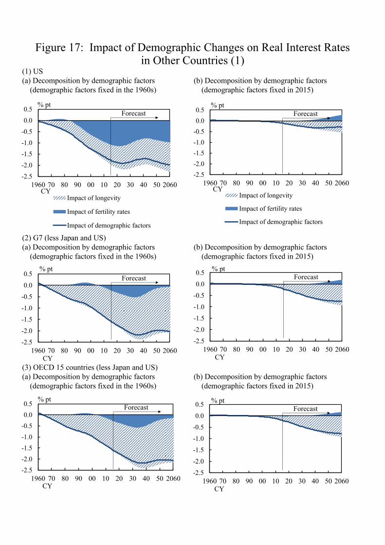
(1) US(a) Decomposition by demographic factors (b) Decomposition by demographic factors (demographic factors fixed in the 1960s) (demographic factors fixed in 2015)

(2) G7 (less Japan and US)(a) Decomposition by demographic factors (b) Decomposition by demographic factors (demographic factors fixed in the 1960s) (demographic factors fixed in 2015)

(3) OECD 15 countries (less Japan and US)(a) Decomposition by demographic factors (b) Decomposition by demographic factors (demographic factors fixed in the 1960s) (demographic factors fixed in 2015)

Figure 17: Impact of Demographic Changes on Real Interest Ratesin Other Countries (1)

-2.5-2.0-1.5-1.0-0.50.00.5

1960 70 80 90 00 10 20 30 40 50 2060

% pt

CY

Forecast

-2.5-2.0-1.5-1.0-0.50.00.5

1960 70 80 90 00 10 20 30 40 50 2060

Impact of longevity

Impact of fertility rates

Impact of demographic factors

% pt

CY

Forecast

-2.5

-2.0

-1.5

-1.0

-0.5

0.0

0.5

1960 70 80 90 00 10 20 30 40 50 2060

% pt

CY

Forecast

-2.5-2.0-1.5-1.0-0.50.00.5

1960 70 80 90 00 10 20 30 40 50 2060

Impact of longevity

Impact of fertility rates

Impact of demographic factors

% pt

CY

Forecast

-2.5

-2.0

-1.5

-1.0

-0.5

0.0

0.5

1960 70 80 90 00 10 20 30 40 50 2060

% pt

CY

Forecast

-2.5

-2.0

-1.5

-1.0

-0.5

0.0

0.5

1960 70 80 90 00 10 20 30 40 50 2060

% pt

CY

Forecast

(1) US(a) Decomposition of labor inputs, level (b) Decomposition of capital inputs, level

(2) G7 (less Japan and US)(a) Decomposition of labor inputs, level (b) Decomposition of capital inputs, level

(3) OECD 15 countries (less Japan and US)(a) Decomposition of labor inputs, level (b) Decomposition of capital inputs, level

Figure 18: Impact of Demographic Changes on Capital and Labor Inputsin Other Countries (2)

-25-20-15-10-505

1960 70 80 90 00 10 20 30 40 50 2060

% deviation

CY

Forecast

Notes: 1. We measure the impact of demographic factors by the discrepancy between the model-generated variable based on the baseline simulation and that based on the counterfactual simulations, where demographic factors (fertility rate, longevity, or both) are held constant at the values of the actual data in the 1960s.

2. The discrepancies are the logarithmic differences of 'baseline simulations' -'counterfactual simulations.'

3. The series are on a per capita basis.

-25-20-15-10-505

1960 70 80 90 00 10 20 30 40 50 2060

Impact of longevity

Impact of fertility rates

Impact of demographic factors

% deviation

CY

Forecast

-25

-20

-15

-10

-5

0

5

1960 70 80 90 00 10 20 30 40 50 2060

% deviation

CY

Forecast

-10-505

101520

1960 70 80 90 00 10 20 30 40 50 2060

Impact of longevity

Impact of fertility rates

Impact of demographic factors

% deviation

CY

Forecast

-10

-5

0

5

10

15

20

1960 70 80 90 00 10 20 30 40 50 2060

% deviation

CY

Forecast

-10-505

101520

1960 70 80 90 00 10 20 30 40 50 2060

% deviation

CY

Forecast

Figure 19: Comparisons of Demographic Variables

020406080

100

1960 70 80 90 00 10 20 30 40 50 2060

ModelData

%

CY

Projection

-4

-2

0

2

4

1960 70 80 90 00 10 20 30 40 50 2060

ModelData

%

Projection

CY

(a) Working-age population growth rate (b) Dependency ratio (1) Japan

020406080

100

1960 70 80 90 00 10 20 30 40 50 2060

ModelData

% Projection

-4

-2

0

2

4

1960 70 80 90 00 10 20 30 40 50 2060

ModelData

%

Projection

(a) Working-age population growth rate (b) Dependency ratio (2) US

020406080

100

1960 70 80 90 00 10 20 30 40 50 2060

ModelData

% Projection

-4

-2

0

2

4

1960 70 80 90 00 10 20 30 40 50 2060

ModelData

%

Projection

(a) Working-age population growth rate (b) Dependency ratio (3) G7 (less US and Japan)

020406080

100

1960 70 80 90 00 10 20 30 40 50 2060

ModelData

% Projection

-4

-2

0

2

4

1960 70 80 90 00 10 20 30 40 50 2060

ModelData

%

Projection

(a) Working-age population growth rate (b) Dependency ratio (4) OECD 15 countries (less US and Japan)

Note: The series of model are model-generated variables based on fertility rates and mortality rates under the baseline simulations. The series of data are the actual figures projected by the respective institutions.

Sources: United Nations, “World Population Prospects”; Census Bureau, “Historical National Population Estimate,” and “2014 to 2060 Populations Projections based on Census 2010”; Social Security Administration, “Life Tables for the United States Social Security Area 1900-2100”; Ministry of Health, Labour and Welfare, “Life Tables“; National Institute of Population and Social Security Research, “Population Projections for

(1) Real interest rate (2) Return on capital

(3) GNP: growth rate (4) Labor inputs: level

(5) Capital inputs: level (6) Saving Rate

on TFP Growth Appendix Figure 1: Simulation under Alternative Assumptions

-4

0

4

8

2000 10 20 30 40 50 2060

TFP -1% GrowthTFP 0% GrowthTFP 2% GrowthTFP 3% GrowthBaseline (1.1%)

%

CY

Forecast

-4

-2

0

2

4

6

2000 10 20 30 40 50 2060

%

CY

Forecast

-15

-10

-5

0

5

10

15

2000 10 20 30 40 50 2060

%

CY

Forecast

0.6

0.7

0.8

0.9

1.0

1.1

2000 10 20 30 40 50 2060

Index: the value as of 2000 under the baseline = 1

CY

Forecast

0

1

2

3

4

5

6

2000 10 20 30 40 50 2060

Index: the value as of 2000 under the baseline = 1

CY

Forecast

1

2

3

4

5

6

7

8

2000 10 20 30 40 50 2060

%

CY

Forecast

Note: The series (3), (4), and (5) are on a per capita basis.

(1) Real interest rate (2) Return on capital

(3) GNP: growth rate (4) Labor inputs: level

(5) Capital inputs: level (6) Saving rate

on Retirement AgesAppendix Figure 2: Simulation under Alternative Assumptions

-4

0

4

8

2000 10 20 30 40 50 2060

Retirement age = 66

Retirement age = 68

Retirement age = 70

%

CY

Forecast

1

2

3

4

5

6

7

8

2000 10 20 30 40 50 2060

%

CY

Forecast

-6

-4

-2

0

2

4

6

2000 10 20 30 40 50 2060

%

CY

Forecast

-2

0

2

4

6

8

10

2000 10 20 30 40 50 2060

%

CY

Forecast

0.6

0.7

0.8

0.9

1.0

1.1

2000 10 20 30 40 50 2060

Index: the value as of 2000 under the baseline = 1

CY

Forecast

0.5

1.0

1.5

2.0

2.5

2000 10 20 30 40 50 2060

Index: the value as of 2000 under the baseline = 1

CY

Forecast

Notes: 1: In each simulation, the retirement age from 1960 to 2015 is 65. In the next five years, the retirement age is assumed to increase to 66, 68, and 70 years gradually, and stays constant after the target age is reached.

2. The series (3), (4), and (5) are on a per capita basis.