bank risk dynamics and distance to default - michigan...
TRANSCRIPT

Bank Risk Dynamics and Distance to Default ∗
Stefan Nagel†
University of Michigan, NBER, and CEPRAmiyatosh Purnanandam‡
University of Michigan
March 2015
Abstract
We adapt structural models of default risk to take into account the special nature of bankassets. The usual assumption of log-normally distributed asset values is not appropriate forbanks. Bank assets are risky debt claims, which implies that they embed a short put optionon the borrowers’ assets, leading to a concave payoff. This has important consequences forbanks’ risk dynamics and distance to default estimation. Due to the payoff non-linearity, bankasset volatility rises following negative shocks to borrower asset values. As a result, standardstructural models in which the asset volatility is assumed to be constant can severely understatebanks’ default risk in good times when asset values are high. Bank equity payoffs resemble amezzanine claim rather than a call option. Bank equity return volatility is therefore much moresensitive to negative shocks to asset values than in standard structural models.
∗We are grateful for conversations with Stephen Schaefer.†Ross School of Business and Department of Economics, University of Michigan, 701 Tappan St., Ann Arbor, MI
48109, e-mail: [email protected]‡Ross School of Business, University of Michigan, 701 Tappan St., Ann Arbor, MI 48109, e-mail: amiy-

I Introduction
The distress that many banks experienced during the recent financial crisis has brought renewed
emphasis on the importance of understanding and modeling bank default risk. Assessment of bank
default risk is important not only from an investor’s viewpoint, but also for risk managers analyzing
counterparty risks and for regulators gauging the risk of bank failure. Accurate modeling of bank
default risk is also required for valuing the benefits that banks derive from implicit and explicit
government guarantees.
In many applications of this kind, researchers and analysts rely on structural models of default
risk in which equity and debt are viewed as contingent claims on the assets of the firm. Following
Merton (1974), the standard approach (which we call the Merton model) is to assume that the value
of the assets of the firm follows a log-normal process. The options embedded in the firm’s equity
and debt can then be valued as in Black and Scholes (1973). In some cases, the distance to default
computed from this model is used as one of the ingredients to empirically model bank default
risk. Recent examples of bank default risk analysis based on the Merton model include Acharya,
Anginer, and Warburton (2014) and Schweikhard, Tsesmelidakis, and Merton (2014), who study
the value of implicit (too-big-to-fail) government guarantees. There is also an extensive literature
that has applied structural models to price deposit insurance, going back to Merton (1977), Marcus
and Shaked (1984), and Pennacchi (1987).
The Merton model’s assumption of log-normally distributed asset values may provide a useful
approximation for the asset value process of a typical non-financial firm. However, for banks this
assumption is clearly problematic. Much of the asset portfolio of a bank consist of debt claims such
as mortgages that involve contingent claims on the assets of the borrower. The fact that the upside
of the payoffs of these debt claims is limited is not consistent with the unlimited upside implied by
a log-normal distribution.
In this paper, we propose a modification of the Merton model that takes into account the debt-
like payoffs of bank assets. Our approach to deal with this problem is to apply the log-normal
distribution assumption not to the assets of the bank, but to the assets of the bank’s borrowers.
More precisely, we model banks’ assets as a pool of loans where borrowers’ loan repayments depend
on the value of their assets at loan maturity as in Vasicek (1991). Borrower asset values are subject
1

0 0.5 1 1.5 20
0.1
0.2
0.3
0.4
0.5
0.6
0.7
0.8
0.9
1
Bank equity
Bank debt
Bank assets
Payo
ff
Borrower asset value
Figure 1: Payoffs at maturity in the simplified model with perfectly correlated borrower defaults
to common factor shocks as well as idiosyncratic risk. We then view the assets of the bank as
contingent claims on borrower assets, and equity and debt of the bank as contingent claims on
these contingent claims.
This options-on-options feature of bank equity and debt has important consequences for the
implied default risk and equity risk dynamics. To illustrate the main intuition, it is useful to
consider the simplified case without idiosyncratic risk in which all borrowers are identical with
perfectly correlated defaults. Assume further that the maturity of the (zero-coupon) debt issued
by the bank equals the maturity of the (zero-coupon) loans made by the bank. In this case, the
payoffs at maturity as a function of borrower asset value are as shown in Figure 1. In this example,
the borrowers have loans with face value 0.80 and the bank has issued debt with face value 0.60.
Since the maximum payoff the bank can receive from the loans is their face value, the bank asset
value is capped at 0.80. Only when borrower assets fall below 0.8 is the bank asset value sensitive
to borrower asset values.
Clearly, the bank asset value cannot follow a log-normal distribution (which would imply un-
limited upside). Since the bank’s borrowers keep the upside of a rise in their asset value above the
loan face value, the bank’s equity payoff does not resemble a call option on an asset with unlimited
2

upside, but rather a mezzanine claim with two kinks. This nature of the banks’ asset payoffs is in
conflict with the assumptions of the standard Merton model.
This mezzanine-like nature of the bank’s equity claim has important consequence for the risk
dynamics of bank equity and for the distance-to-default estimation. Due to the capped upside,
bank volatility will be very low in “good times” when asset values are high and it is likely that
asset values at maturity will end up towards the right side in Figure 1 where the bank’s equity
payoff is insensitive to fluctuations in borrower asset values.
A standard Merton-model in which equity is a call option on an asset with constant volatility
misses these nonlinear risk dynamics. Viewed through the lens of this standard model it might seem
that a bank in times of high asset values is many standard deviations away from default. But this
conclusion would be misleading because it ignores the fact that volatilities could rise dramatically
if asset values fall. Similarly, the standard model would give misleading predictions about the
riskiness of bank assets, equity, and debt.
Going beyond this simple illustrative example, our model incorporates additional features such
as idiosyncratic borrower risks, staggered remaining loan maturities, and the replacement of ma-
turing loans with new loans. While these generalizations are important to get a more realistic
model that we can use for a quantitative evaluation of bank risk, the addition of these features does
not change the basic insight about the mezzanine-claim nature of bank equity and the resulting
consequences for risk dynamics and distance to default.
To assess the differences between our modified model and the Merton model, we simulate data
from our modified model and ask to what extent an analyst using the Merton model would mis-
judge the risk-neutral probability of default. We find that this error is particularly stark when asset
values are high relative to the face value of the bank’s debt. In this case, bank asset payoffs are
likely to stay in the flat region in Figure 1 and bank equity payoffs are also likely in the flat region.
As a consequence, equity volatility is low. Based on the Merton model, an analyst observing low
equity volatility would infer that asset volatility must be low. Furthermore, since asset volatility
is constant in the Merton model, the analyst would (wrongly) conclude that asset volatility will
remain low at this level in the future. What the Merton model misses in this case is that asset
volatility could rise substantially following a bad asset value shock, because the region of likely
asset payoffs would move closer to or into the downward sloping region in Figure 1. As a result,
3

the Merton model substantially overestimates the distance to default and it underestimates the
risk-neutral probability of default.
We then calibrate our modified model and the standard Merton model to quarterly bank panel
data from 2002 to 2012. We choose the value and volatility of bank assets (in the case of the Merton
model) or borrower assets (in case of our modified model) to match the observed market value of
equity and its volatility. Even though both models are calibrated to the same data, their implied
risk-neutral default probabilities are strikingly different. In line with the simulations we discussed
above, the differences are particularly big in the years before the financial crisis when equity values
were high and volatility low. Based on the Merton model, the risk-neutral default probability of the
average bank in 2006 over a 5-year horizon is less than 10%. In contrast, the risk-neutral default
probability from our modified model is two to three times as high. Translated into credit spreads,
this would imply an annualized spread of around 10 basis points in the Merton model and close to
100 basis points according to our modified model.
Once the financial crisis hit in 2007/08, the models’ predictions are not so different anymore. At
this point, bad asset value shocks had moved banks into the downward-sloping asset payoff region
in Figure 1. In this region, the kink in the asset payoff becomes less relevant and the predictions
from our modified model are close to those from the standard Merton model. In periods of the
most extreme distress, Merton model default probabilities can even exceed those from our modified
model.
Thus, the key problem with applications of standard structural models to banks is that they
understate the risk of default in “good times.” This is an important issue, for example, for the
estimation of the value of explicit or implicit government guarantees. Based on a standard Merton
model calibrated to equity value and volatility data from 2006 (i.e., pre-crisis times), one may be
lead to the conclusion that the value of a guarantee is almost nil when, in fact, the value is a lot
higher if one takes into account that banks’ asset volatility will go up when asset values fall.
We further investigate the plausibility of our modification of the Merton model by comparing
the models’ predictions about bank equity volatility following a bad shock to the bank’s asset value.
We calibrate both models to match data on equity values and volatility in 2006Q2. We then add a
negative shock to borrower asset values based on the change in U.S. house prices from 2006Q2 to
subsequent quarters. The negative shock to borrower asset values then translates, in our modified
4
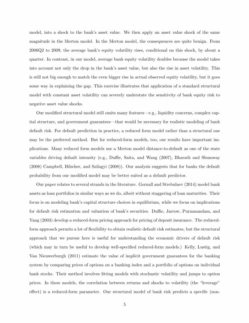
model, into a shock to the bank’s asset value. We then apply an asset value shock of the same
magnitude in the Merton model. In the Merton model, the consequences are quite benign. From
2006Q2 to 2009, the average bank’s equity volatility rises, conditional on this shock, by about a
quarter. In contrast, in our model, average bank equity volatility doubles because the model takes
into account not only the drop in the bank’s asset value, but also the rise in asset volatility. This
is still not big enough to match the even bigger rise in actual observed equity volatility, but it goes
some way in explaining the gap. This exercise illustrates that application of a standard structural
model with constant asset volatility can severely understate the sensitivity of bank equity risk to
negative asset value shocks.
Our modified structural model still omits many features—e.g., liquidity concerns, complex cap-
ital structure, and government guarantees—that would be necessary for realistic modeling of bank
default risk. For default prediction in practice, a reduced form model rather than a structural one
may be the preferred method. But for reduced-form models, too, our results have important im-
plications. Many reduced form models use a Merton model distance-to-default as one of the state
variables driving default intensity (e.g., Duffie, Saita, and Wang (2007), Bharath and Shumway
(2008) Campbell, Hilscher, and Szilagyi (2008)). Our analysis suggests that for banks the default
probability from our modified model may be better suited as a default predictor.
Our paper relates to several strands in the literature. Gornall and Strebulaev (2014) model bank
assets as loan portfolios in similar ways as we do, albeit without staggering of loan maturities. Their
focus is on modeling bank’s capital structure choices in equilibrium, while we focus on implications
for default risk estimation and valuation of bank’s securities. Duffie, Jarrow, Purnanandam, and
Yang (2003) develop a reduced-form pricing approach for pricing of deposit insurance. The reduced-
form approach permits a lot of flexibility to obtain realistic default risk estimates, but the structural
approach that we pursue here is useful for understanding the economic drivers of default risk
(which may in turn be useful to develop well-specified reduced-form models.) Kelly, Lustig, and
Van Nieuwerburgh (2011) estimate the value of implicit government guarantees for the banking
system by comparing prices of options on a banking index and a portfolio of options on individual
bank stocks. Their method involves fitting models with stochastic volatility and jumps to option
prices. In these models, the correlation between returns and shocks to volatility (the “leverage”
effect) is a reduced-form parameter. Our structural model of bank risk predicts a specific (non-
5

linear) relation between bank equity returns and bank equity volatility.
The rest of the paper is organized as follows. Section II presents our modified model and
simulations to illustrate the key differences to the standard Merton model. In Section III we apply
the model to empirical bank panel data and we analyze the resulting estimates of default risk.
Section IV discusses implications for reduced form models of default risk. Section V concludes.
II Structural Model of Default Risk for Banks
Unlike the simplified case in Figure 1, we now set up a model in which borrower asset have idiosyn-
cratic risk and banks issue loans with staggered maturities. Both of these additional features are
important because they lead to some smoothing of the bank asset payoff function in Figure 1.
Consider a setting with continuous time. A bank issues zero-coupon loans with maturity T .
Loans are issued in staggered fashion to N cohorts of borrowers. Cohorts are indexed by τ =
T, T (N − 1)/N, ..., 1/N , the remaining maturity on their loans at t = 0. These loans were issued
at τ − T with face value F1. Each cohort is comprised of a continuum of borrowers indexed by
i ∈ [0, 1] with mass 1/N .
Let Aτ,it denote the collateral value of a borrower i in cohort τ at time t. Under the risk-neutral
measure, the asset value evolves according to the stochastic differential equation
dAτ,it
Aτ,it= (r − δ)dt+ σ(
√ρdWt +
√1− ρdZτ,it ), (1)
where W and Zτ,i are independent standard Brownian motions, δ is a depreciation rate, and r is
risk-free rate. The Zτ,i processes are idiosyncratic and independent across borrowers. This is a
one-factor model of borrower asset values as in Vasicek (1991). The parameter ρ represents the
correlation of asset values that arises from common exposure to W .
At the time of the initial loan issue, τ−T , borrowers’ collateral is normalized to Aτ,iτ = 1. Thus,
the initial loan-to-value ratio is
` = F1e−µT , (2)
with µ as the promised yield on the loan (that we will solve for below). In line with standard
structural models of credit risk, we assume that borrowers default if the asset value at maturity is
6
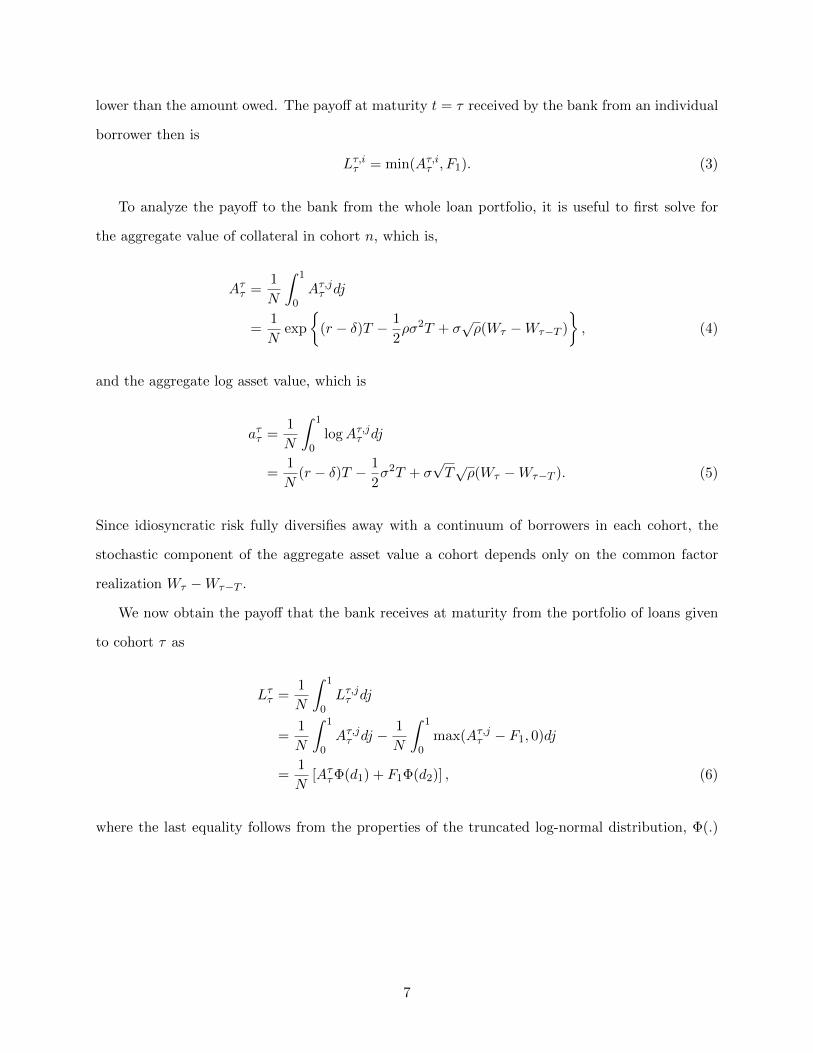
lower than the amount owed. The payoff at maturity t = τ received by the bank from an individual
borrower then is
Lτ,iτ = min(Aτ,iτ , F1). (3)
To analyze the payoff to the bank from the whole loan portfolio, it is useful to first solve for
the aggregate value of collateral in cohort n, which is,
Aττ =1
N
∫ 1
0Aτ,jτ dj
=1
Nexp
{(r − δ)T − 1
2ρσ2T + σ
√ρ(Wτ −Wτ−T )
}, (4)
and the aggregate log asset value, which is
aττ =1
N
∫ 1
0logAτ,jτ dj
=1
N(r − δ)T − 1
2σ2T + σ
√T√ρ(Wτ −Wτ−T ). (5)
Since idiosyncratic risk fully diversifies away with a continuum of borrowers in each cohort, the
stochastic component of the aggregate asset value a cohort depends only on the common factor
realization Wτ −Wτ−T .
We now obtain the payoff that the bank receives at maturity from the portfolio of loans given
to cohort τ as
Lττ =1
N
∫ 1
0Lτ,jτ dj
=1
N
∫ 1
0Aτ,jτ dj − 1
N
∫ 1
0max(Aτ,jτ − F1, 0)dj
=1
N[AττΦ(d1) + F1Φ(d2)] , (6)
where the last equality follows from the properties of the truncated log-normal distribution, Φ(.)
7

denotes the standard normal CDF, and
d1 =logF1 − aττ√
1− ρ√Tσ−√
1− ρ√Tσ, (7)
d2 = − logF1 − aττ√1− ρ
√Tσ
. (8)
The max(Aτ,jτ − F1, 0) term in (6) reflects the option value for the borrower, i.e., the upside of
the collateral value that is retained by the borrower. Conditional on Wτ −Wτ−T , there are some
borrowers in cohort τ for whom this option is in the money, and others for whom it is not, depending
on the realization of the idiosyncratic shock. This is why d1 and d2 are functions of idiosyncratic
risk√
1− ρ√Tσ. Thus, while idiosyncratic risk is diversified away in the aggregate borrower asset
value, it matters for loan payoffs, because borrower default depends on idiosyncratic risk.
We assume that loans are priced competitively, and so the promised yield on the loan can now
be found as the µ that solves
F1e−µT = e−rTEQ
τ−T [Lnτ ], (9)
where EQt [.] denotes a conditional expectation under the risk-neutral measure. The risk-neutral
expectation on the right-hand side can be evaluated by simulating the distribution of Lττ , based on
(6) and the simulated distribution of Anτ , under the risk-neutral measure.
At t = τ , the bank fully reinvests the proceeds , Lττ , from the maturing loan portfolio of cohort
τ into new loans, with uniform amounts, to members of the same cohort. The new loans carry a
face value of
F2 = LττeµT . (10)
We assume that the bank keeps the time-of-issue loan-to-value ratio at the same level, i.e., `, as
for the initial round of loans. Borrowers reduce or replenish collateral assets accordingly: the asset
value of each member of cohort τ is reset to the same value
Aτ,iτ+
=Lττ`
(11)
an instant after the re-issue of the loans. The cohort-level aggregates Aτt and aτt for t > τ are based
8

on these re-initialized asset values.
The aggregate payoff of the portfolio of loans of cohort τ at the subsequent maturity date τ +T
then follows, along similar lines as above, as
Lττ+T =1
N
∫ 1
0Lτ,jτ+Tdj
=1
N
∫ 1
0Aτ,jτ+Tdj −
1
N
∫ 1
0max(Aτ,jτ+T , 0)dj
=1
N
[Aττ+TΦ(d3) + F2Φ(d4)
](12)
where
d3 =logF2 − anτ+T√
1− ρ√Tσ
−√
1− ρ√Tσ, (13)
d4 = −logF2 − anτ+T√
1− ρ√Tσ
. (14)
Thus, after the roll-over into new loans, there are two state variables to keep track off that Aττ+T
and F2 depend on: First, the change of the common factor since roll-over, Wt −Wτ , and second,
Lττ , which in turn is driven by Wτ −Wτ−T .
The payoffs in (12) and (6) together allow us to describe the distribution of the bank’s assets.
Consider, for example, the aggregate value of the bank’s loan portfolio at t = H, where H < T .
Aggregating across all loans outstanding at this time, we get
VH =∑τ<H
e−r(τ+T−H)EQH [Lττ+T ] +
∑τ≥H
e−r(τ−H)EQH [Lττ ], (15)
where the first term aggregates over cohorts whose loans have been rolled over into a second round,
while the term aggregates over cohorts that still have the initial first-round loans outstanding.
Substituting in from (6) and (12) yields an expression in which the only source of stochastic shocks
is the common factor W . Therefore, by simulating W we can simulate the distribution of VH and
price contingent claims whose payoffs are functions of VH .
Figure 2 shows the simulated bank asset value, VH , based on 10,000 draws of the common factor
paths plotted against the aggregate borrower asset value at t = H. Parameters are set at H = 5,
9

0 0.2 0.4 0.6 0.8 1 1.2 1.4 1.6 1.8 20
0.1
0.2
0.3
0.4
0.5
0.6
0.7
0.8
0.9
1
Bank
ass
et v
alue
Aggregate borrower asset value
Figure 2: Bank asset value at bank debt maturity as a function of aggregate borrower asset value.Simulated bank asset values shown as dots. Dashed line shows the kinked payoff that would resultwith perfectly correlated borrower asset values and without staggering of loan maturities
T = 10, σ = 0.2, ρ = 0.5, r = 0.01, δ = 0.005, and F1 = 0.8. Unlike in Figure 1, there is no sharp
kink in the bank’s asset value in Figure 2 . There are two reasons for the lack of sharp kink. First,
in this case, loans in the bank’s portfolio are not at maturity. For H < τ ≤ T , loans have not
matured yet, while for 0 ≤ τ < H, they have been rolled over into new loans. Second, the existence
of idiosyncratic borrower risk makes the borrower’s default option more valuable and the loan less
valuable to the bank, particularly when the asset value is close to the face value of the debt.
Moreover, unlike in Figure 1, there is dispersion in the bank asset value conditional on the
aggregate borrower asset value. The reason is that for loans that have been rolled over into a
second generation of loans, the face value of the loan depends on the common factor realization up
to the roll-over date τ . For example, if Wτ is low, there will be more defaults at τ and hence the
face value of new loans will be lower than if Wτ is high.
V0, the total market value of the bank’s assets at t = 0 can be computed as
V0 = e−rHEQ0 [VH ] (16)
10
0 0.5 1 1.5 2 2.50
0.02
0.04
0.06
0.08
0.1
0.12
0.14
0.16
Bank
equ
ity v
alue
Aggregate borrower asset value
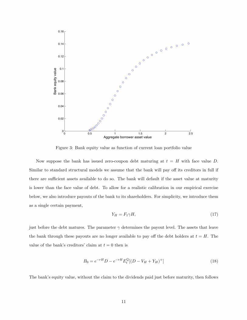
Figure 3: Bank equity value as function of current loan portfolio value
Now suppose the bank has issued zero-coupon debt maturing at t = H with face value D.
Similar to standard structural models we assume that the bank will pay off its creditors in full if
there are sufficient assets available to do so. The bank will default if the asset value at maturity
is lower than the face value of debt. To allow for a realistic calibration in our empirical exercise
below, we also introduce payouts of the bank to its shareholders. For simplicity, we introduce them
as a single certain payment,
YH = F1γH, (17)
just before the debt matures. The parameter γ determines the payout level. The assets that leave
the bank through these payouts are no longer available to pay off the debt holders at t = H. The
value of the bank’s creditors’ claim at t = 0 then is
B0 = e−rHD − e−rHEQt [(D − VH + YH)+] (18)
The bank’s equity value, without the claim to the dividends paid just before maturity, then follows
11

0 0.5 1 1.5 2 2.50
0.2
0.4
0.6
0.8
1
1.2
1.4
1.6
1.8
Inst
. ban
k eq
uity
vol
.
Current loan portfolio value
Figure 4: Instantaneous bank equity volatility as function of current loan portfolio value
as
S0 = V0 − e−rHYH −B0 (19)
Figure 3 shows simulation results for the relationship between S0 and V0. We use the same
parameters as in Figure 2 and D = 0.6, YH = 0.008. To explore the effect of changes in borrower
asset value, we set common factor shocks until t = 0 to zero, and we then apply a single shock
dW0 to all cohorts and then simulate W going forward. We vary dW0 from −0.8 to 0.8 across
simulations. As a consequence, we generate variation in bank asset values across simulations.
As Figure 3 shows, the value of bank equity is concave in bank assets for large values. This is
in contrast to the standard Merton model in which the equity value asymptotes towards a slope of
one. Thus, we get a similar mezzanine-like payoff for bank equity as in our preliminary analysis in
Figure 1, albeit with smoothed kinks.
Figure 4 shows the instantaneous volatility of the bank’s equity. Given knowledge of the pa-
rameters, one can numerically compute the instantaneous equity volatility from the first derivative
of S0 with respect to W0. Since common factor shocks are the only source of stochastic shocks to
12

the bank asset value, this derivative with respect to W0 is directly related to the slope of the curve
in Figure 3. As Figure 4 shows, equity volatility converges towards zero for high bank asset values.
In the Merton model, in contrast, equity volatility would asymptote towards the (strictly positive)
volatility of assets.
This very low equity volatility at high asset values arises from the mezzanine-claim nature
of bank equity. Positive shocks to asset values raise borrower asset values far above the default
thresholds. As a result, bank assets have very low instantaneous risk in good times and bank
equity risk resembles the risk of a bond because the region of concavity dominates. Application
of a standard Merton model with log-normal asset value would miss this non-linearity in bank’s
equity risk. Our modified model suggests that this non-linearity is a key property of bank equity
risk dynamics.
In particular, our model makes clear that low instantaneous bank equity volatility in good
times can quickly turn into high risk in bad times if asset values fall. In the standard model with
a log-normal asset value, the rise in bank equity volatility with a fall in asset values is moderate
because bank asset volatility is fixed. In our modified model, bank asset volatility goes up as loans
fall in value and become riskier. The rise in equity volatility following bad shocks is therefore more
dramatic than in the standard Merton model.
II.A Default Risk Assessment: Comparison with Standard Merton Model
The highly nonlinear relation between bank asset value and bank equity risk due to the short put
option embedded in bank assets leads to important consequences for distance to default estimation
and empirical assessment of default risk. To illustrate these consequences, we now analyze a setting
in which our modified model represents the true data generating process. We simulate from our
model with parameter values set to the same values as above in Figure 3. We then study to what
extent an analyst applying the (misspecified) standard Merton model would arrive at misleading
conclusions about bank default risk.
Figure 5 shows the simulated actual risk-neutral default probabilities in our model (blue) and
those estimated based on the Merton model (red) applied to our simulated data. The Merton
model default probabilities are obtained by using the simulated equity values and instantaneous
volatilities to extract asset values and asset volatilities under the (false) assumption of a log-normal
13

0 0.5 1 1.5 2 2.50
0.1
0.2
0.3
0.4
0.5
0.6
0.7
0.8
0.9
1
Aggregate borrower asset value
RN
ban
k de
faul
t pro
babi
lity
ActualMerton Model
Figure 5: Risk-neutral default probabilities as function of current loan portfolio value: Merton(red) and modified (blue)
asset value process (see Appendix A). This corresponds to the practice of applying the Merton
model to recent empirical volatilities and observed equity values. As the Figure shows, the Merton
model underestimates the probability of default for moderate (and, in most cases, more realistic)
default probabilities. In these good states of the world, the default probabilities are massively
understated when the (misspecified) Merton model is applied. If the borrower asset values are
relatively high, bank equity volatility is very low because bank asset volatility is very low. However,
asset volatility could quickly rise if asset values fall, which means that it is much more likely than
one would think based on the Merton model that the default threshold could be reached. Low
instantaneous equity volatility hence does not mean that the bank operates at a high distance to
default. However, an analyst applying the standard Merton model with constant asset volatility
would miss these nonlinear risk dynamics. Within the standard Merton model, the analyst would
interpret the low instantaneous equity volatility as a high distance to default and hence low default
risk. Thus, particularly in good times, application of the Merton model is likely to lead to severe
underestimation of bank default risk. Only in a severely distressed situation, when asset values are
14

0 0.5 1 1.5 2 2.50
0.005
0.01
0.015
0.02
0.025
0.03
0.035
0.04
0.045
0.05
Aggregate borrower asset value
Cre
dit s
prea
d
ActualMerton Model
Figure 6: Implied credit spread: Merton (red) and modified (blue)
depressed and default is almost certain, the Merton model slightly overstates risk-neutral default
probabilities. Here the above effect works in reverse.
Figure 6 presents the implied credit spread of the bank’s 5-year debt. The credit spread reflects
the product of the risk-neutral probability of default (as shown in Figure 5) and the loss given default
(which equals one minus the recovery rate), shown on an annualized basis. Since the recovery rate
in a Merton style model can often be quite high in cases where the asset value at maturity ends up
only slightly below the face value of the debt, the implied credit spreads are much lower than the
risk-neutral default probabilities. Our main focus is again on how an analyst using the standard
Merton model would severely underestimate credit spreads. For example, when borrower asset
values are around one, and hence substantially above the face value of their loans, the bank’s credit
spread according to the Merton model should be about 10 basis points. In contrast, the true credit
spread is close to 1% and hence almost an order of magnitude bigger.
Figure 7 shows how application of the standard Merton model would severely estimate the value
of a government guarantee. For illustration, we suppose that there is a 50% risk-neutral probability
that the government will fully bail out the debt holders (and absorb the entire loss given default)
15

0 0.5 1 1.5 2 2.50
0.005
0.01
0.015
0.02
0.025
0.03
Aggregate borrower asset value
Valu
e of
gov
ernm
ent g
uara
ntee
ActualMerton Model
Figure 7: Value of a government guarantee: Merton (red) and modified (blue)
in the event of default. The value of the government guarantee then is 0.5 times the value of
the bank’s default option. To interpret the magnitudes in Figure 7, recall that the aggregate face
value of the bank’s loans in our simulations is around 0.80. As the figure shows, application of the
standard Merton model would severely underestimate the value of the guarantee. For aggregate
borrower asset values around one, the value of the guarantee is about 0.0015, i.e., about 0.2% of
the face value of the bank’s loan portfolio, while the actual value is almost ten times as big.
III Empirical Calibration
To find out how much, quantitatively, the standard Merton model and our modified model differ
in their predictions about default probabilities and risk dynamics, we now calibrate these models
with empirical data on bank’s capital structures and equity volatility.
16
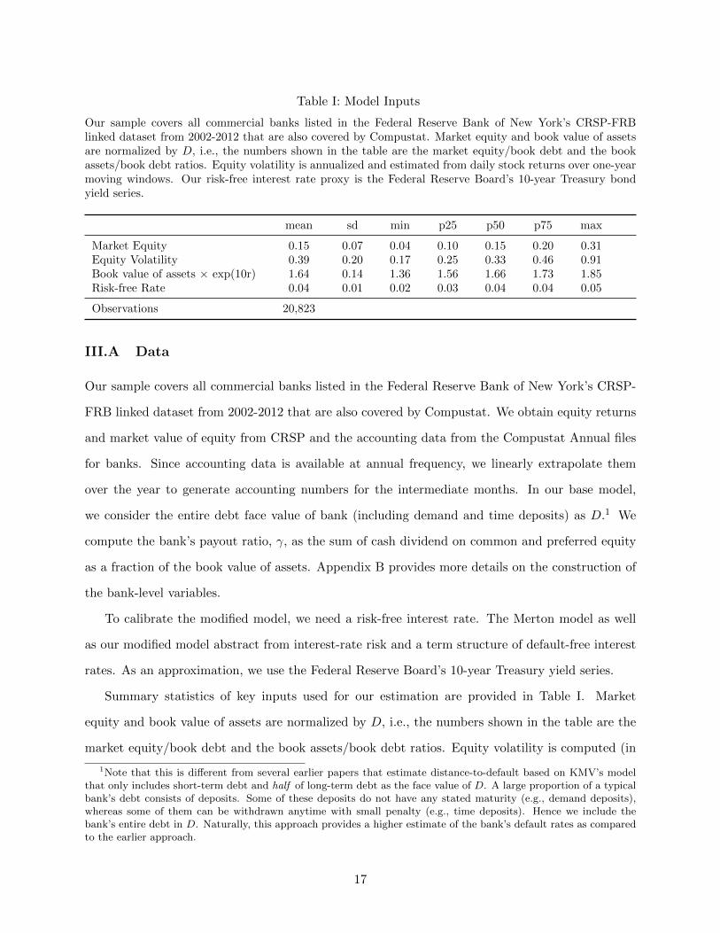
Table I: Model Inputs
Our sample covers all commercial banks listed in the Federal Reserve Bank of New York’s CRSP-FRBlinked dataset from 2002-2012 that are also covered by Compustat. Market equity and book value of assetsare normalized by D, i.e., the numbers shown in the table are the market equity/book debt and the bookassets/book debt ratios. Equity volatility is annualized and estimated from daily stock returns over one-yearmoving windows. Our risk-free interest rate proxy is the Federal Reserve Board’s 10-year Treasury bondyield series.
mean sd min p25 p50 p75 max
Market Equity 0.15 0.07 0.04 0.10 0.15 0.20 0.31Equity Volatility 0.39 0.20 0.17 0.25 0.33 0.46 0.91Book value of assets × exp(10r) 1.64 0.14 1.36 1.56 1.66 1.73 1.85Risk-free Rate 0.04 0.01 0.02 0.03 0.04 0.04 0.05
Observations 20,823
III.A Data
Our sample covers all commercial banks listed in the Federal Reserve Bank of New York’s CRSP-
FRB linked dataset from 2002-2012 that are also covered by Compustat. We obtain equity returns
and market value of equity from CRSP and the accounting data from the Compustat Annual files
for banks. Since accounting data is available at annual frequency, we linearly extrapolate them
over the year to generate accounting numbers for the intermediate months. In our base model,
we consider the entire debt face value of bank (including demand and time deposits) as D.1 We
compute the bank’s payout ratio, γ, as the sum of cash dividend on common and preferred equity
as a fraction of the book value of assets. Appendix B provides more details on the construction of
the bank-level variables.
To calibrate the modified model, we need a risk-free interest rate. The Merton model as well
as our modified model abstract from interest-rate risk and a term structure of default-free interest
rates. As an approximation, we use the Federal Reserve Board’s 10-year Treasury yield series.
Summary statistics of key inputs used for our estimation are provided in Table I. Market
equity and book value of assets are normalized by D, i.e., the numbers shown in the table are the
market equity/book debt and the book assets/book debt ratios. Equity volatility is computed (in
1Note that this is different from several earlier papers that estimate distance-to-default based on KMV’s modelthat only includes short-term debt and half of long-term debt as the face value of D. A large proportion of a typicalbank’s debt consists of deposits. Some of these deposits do not have any stated maturity (e.g., demand deposits),whereas some of them can be withdrawn anytime with small penalty (e.g., time deposits). Hence we include thebank’s entire debt in D. Naturally, this approach provides a higher estimate of the bank’s default rates as comparedto the earlier approach.
17

Table II: Parameters
Parameter Description Value
δ Borrower Asset Depreciation Rate 0.005γ Bank payout Rate 0.002T Bank Loan Maturity 10 yearsH Bank Debt Maturity 5 yearsρ Borrower asset value correlation 0.5
` Loan-to-Value Ratio 0.8e(µ−r)T
annualized form) from daily bank stock returns over one-year moving windows.
III.B Model calibration
For both the standard Merton model and our modified model, we set the maturity of bank debt
to H = 5. It is well known that models with only diffusive shocks do not succeed in delivering
realistic default risk and credit spread predictions for short-term debt (Duffie and Lando (2001),
Zhou (2001)). Our modified model is no different. At short horizons, therefore, differences between
our modified model and the standard model are also relatively small. The non-linearity in banks’
asset payoffs becomes more relevant as the probability distribution of borrower asset values spreads
out with longer horizons. Longer horizons may also be relevant even for investors in short-term
debt (or guarantors of short-term debt). Solvency problems may not be immediately apparent
when bad shocks are realized. Deterioration in asset values may be hidden for a while, perhaps
facilitated by regulatory forbearance, and short-term debt may be rolled over even if the bank is
actually insolvent. By the time default happens, additional losses may have accumulated.
We calibrate the standard Merton model by simultaneously solving for asset value and asset
volatility that deliver the observed values of a bank’s equity and stock return volatility (see Ap-
pendix A). This approach has been used by prior researchers such as Campbell, Hilscher, and
Szilagyi (2008) and Acharya, Anginer, and Warburton (2014). We solve the model quarterly from
2002 to 2012. We use the equity value as of the beginning of the quarter and compute the standard
deviation of equity returns based on trailing 12 months of return data.
For our modified model, we have several additional parameters that we fix exogenously, as
shown in Table II. We set the depreciation rate δ = 0.005. We assume that the maturity of loans
issued by banks is T = 10 and that borrower asset values have a pairwise correlation of ρ = 0.5.
18

Table III: Model-Implied Risk-Neutral Probabilities of Default
We calibrate the Merton model and our modified model quarterly from 2002-2012 based on the data summa-
rized in Table I. For each bank in each calibration period, we compute the risk-neutral default probability
from the two models. The table reports summary statistics for these risk-neutral default probabilities for
the whole panel of banks over the full sample period.
mean sd min p25 p50 p75 max
Merton Model RN prob(default) 0.26 0.27 0.01 0.05 0.15 0.39 0.89Modified Model RN prob(default) 0.34 0.21 0.00 0.17 0.35 0.52 0.70
Observations 20,823
This correlation assumption is not crucial. A lower ρ implies more smoothing of the kinks in the
payoff function in Figure 2, but otherwise its effects are limited because any change in ρ requires an
offsetting change in σ when we calibrate the model to match observed equity value and volatility.
We set γ equal to the observed payout rate of the bank.
We normalize D = 1. The face value of the loans in the bank’s portfolio represents, roughly,
the book assets of the bank. To take into account the zero-coupon nature of the loans, we adjust
the book value for the time until loan maturity and we set F1 equal to the inverse of the observed
book leverage times exp(10r). We then look for values of dW0 and σ that allow us to match the
empirically observed equity value and equity volatility (over a 12-month backward looking window)
of the bank with the model implied value.
III.C Model-implied risk-neutral default probabilities
Table III gives the summary statistics of the two calibrated models’ implied risk-neutral default
probabilities (RNPD) for our panel of banks. We calibrate each model quarterly from 2002-2012.
The average RNPD is slightly higher in our modified model compared with the standard Merton
model. However, the Merton model RNPD is much more positively skewed. The reason is that
when a bank is not in distress, the implied RNPD in the Merton model is very low because it is
based on the assumption that the bank’s assets have constant volatility. In contrast, our model
takes into account that bad shocks to asset values in the future would drive up the volatility of the
bank’s assets (as borrower’s default options move into the money), which drastically shrinks the
distance to default and hence raises the RNPD in times when asset values are relatively high.
19

02Q1 04Q1 06Q1 08Q1 10Q1 12Q10
0.1
0.2
0.3
0.4
0.5
0.6
0.7
0.8
0.9
Year−Quarter
RN
ban
k de
faul
t pro
babi
lity
ModifiedMerton Model
Figure 8: Comparison of calibrated risk-neutral default probabilities (5-year horizon, cumulative)
20

Figure 8 further illustrates the different behavior of the RNPD from the two models in good
times and bad times. The figure shows the average RNPD across all banks each quarter from
2002-2012. The modified model’s RNPD is two to three times as high as Merton RNPD during
the time before the financial crisis. Expressed in terms of annualized credit spreads, these RNPD
in 2006 would correspond, roughly, to 10 basis points for the Merton model and close to 100 basis
points for our modified model.
This behavior of the relative RNPDs is in line with the intuition that bank assets have nonlinear
debt-like payoffs. In good times, the Merton model’s assumption of constant asset volatility pro-
duces very high distance to default and low RNPD. In our model, the analysis recognizes that the
volatility of bank assets in good times (in the flat part of the concave asset payoff region in Figure
2) is low, but that it can quickly rise after a bad shock (when the bank gets into the downward
sloping asset payoff region). Once the asset value has suffered a sufficiently big bad shock, the
asset payoff is dominated by the linear downward sloping region and the kink is not playing much
of a role. In this case, the predictions of the Merton model and our modified model are relatively
similar. This is why after the onset of the financial crisis in 2007, the difference between the RNPD
shrinks and eventually inverts in 2008.
We further illustrate this cyclical behavior of the RNPD differences between the Merton model
and our modified model with the following panel regression
logRNPDModified
it
RNPDMertonit
= αi + β1 × LowV IXt + β2 × logEit + β3 × LowV IXt × logEit + εit (20)
The dependent variable is the log difference in default probabilities for a bank i in quarter t. VIX is
the CBOE index of implied volatilities on S&P500 index options. LowVIX equals one for quarters
with below median VIX, zero otherwise. E measures each bank’s market equity (normalized by to
total debt, as in Table I). The regression results in Table IV show that the modified model RNPD is
significantly higher during “quiet” periods, and for high equity banks. Column (IV) further shows
the interaction effect: The standard Merton model delivers a lower default probability for banks
with higher equity during low VIX periods.
Table V presents results of a similar regression model, but with the level of the S&P500 index
during our sample period as the measure of good/bad times.
21

Table IV: Differences in Model-Implied Risk-Neutral Default Probability: Comparison BetweenHigh- and Low-VIX Periods
The dependent variable is the log risk-neutral default probability from our modified model minus the log
risk-neutral default probability from the standard Merton model for our panel of banks from 2002-2012.
Explanatory variables include a dummy for quarters with below median VIX index, and the bank’s log
market equity (normalized by to total debt, as in Table I).
I II III IV V
Low VIX 0.569∗∗∗ 0.372∗∗∗ 1.822∗∗∗ 0.000(0.00) (0.00) (0.00) (.)
Equity 0.873∗∗∗ 0.734∗∗∗ 0.386∗∗∗ -0.064(0.00) (0.00) (0.00) (0.33)
Low VIX x Equity 0.717∗∗∗ 0.709∗∗∗
(0.00) (0.00)
Constant 0.118∗∗∗ 2.182∗∗∗ 1.698∗∗∗ 0.946∗∗∗ -0.153(0.00) (0.00) (0.00) (0.00) (0.26)
YQ Fixed Effect No No No No Yes
Observations 19,297 19,297 19,297 19,297 19,297R2 0.236 0.259 0.272 0.288 0.328Absorbed FE Bank Bank Bank Bank BankClustered by Bank Bank Bank Bank Bank
p-values in parentheses∗ p < 0.10, ∗∗ p < 0.05, ∗∗∗ p < 0.01
logRNPDModified
it
RNPDMertonit
= αi + β1 ×HighS&Pt + β2 × logEit + β3 ×HighS&Pt × logEit + εit (21)
HighS&P equals one for quarters with above median level of S&P500 index, zero otherwise. The
regression results show that the modified model RNPD is significantly higher during periods with
high stock market valuation, and for high equity banks. Column (IV) further shows the interaction
effect: The standard Merton model implies a lower default probability for banks with higher equity
during periods in which the S&P500 index is high.
III.D Model-implied equity risk dynamics
The motivation for our modification of the standard Merton model is based on a priori reasoning
that the nature of bank asset payoffs is fundamentally inconsistent with a log-normal process.
Improving the model on this dimension seems of first-order importance and should lead to an
22

Table V: Differences in Model-Implied Risk-Neutral Default Probability: Comparison BetweenHigh- and Low-Stock Market Index Periods
The dependent variable is the log risk-neutral default probability from our modified model minus the log
risk-neutral default probability from the standard Merton model for our panel of banks from 2002-2012.
Explanatory variables include a dummy for quarters with below median S&P 500 Index and the bank’s log
market equity (normalized by to total debt, as in Table I).
I II III IV V
High S&P Level 0.135∗∗∗ 0.101∗∗∗ 0.683∗∗∗ 0.000(0.00) (0.00) (0.00) (.)
Equity 0.873∗∗∗ 0.868∗∗∗ 0.730∗∗∗ -0.069(0.00) (0.00) (0.00) (0.34)
High S&P Level x Equity 0.290∗∗∗ 0.595∗∗∗
(0.00) (0.00)
Constant 0.362∗∗∗ 2.182∗∗∗ 2.120∗∗∗ 1.841∗∗∗ -0.161(0.00) (0.00) (0.00) (0.00) (0.27)
YQ Fixed Effect No No No No Yes
Observations 19,297 19,297 19,297 19,297 19,297R2 0.204 0.259 0.260 0.262 0.325Absorbed FE Bank Bank Bank Bank BankClustered by Bank Bank Bank Bank Bank
p-values in parentheses∗ p < 0.10, ∗∗ p < 0.05, ∗∗∗ p < 0.01
improvement in the empirical performance of the model. At the same time, it is clear that even the
modified model, in this simple form, is likely to miss important features of a bank’s capital structure
and of how a distressed bank enters into default. Among other things, our modified model does not
take into account the presence of implicit and explicit government guarantees. Furthermore, bank
capital structures are a lot more complex than our simple model allows for. A direct comparison
of the model implied RNPD with bank CDS rates or credit spreads would therefore difficult to
interpret.
At this point, we do not focus on refining the model to account for these additional complexities,
but rather to evaluate, with a broad brush, the plausibility of our modification of the Merton model.
To do so, we focus on the dynamics of bank equity risk. The risk of the equity claim should be
less sensitive to government guarantees and interventions than default risk measures, as their main
effect is on the more senior claims in a bank’s capital structure.
The modified model and the standard model differ starkly in their predictions of how bank
23

equity risk responds to asset value shocks. To study these differences, we subject bank asset values
to a realistic negative asset value shock. We then calculate the models’ equity volatility predictions,
conditional on this shock, and we compare these predictions with actual data on the trajectory of
bank equity volatilities going into the financial crisis around 2008/09. In the standard model, a
shock to a bank’s asset value leaves the asset volatility unchanged. In contrast, in our modified
model a shock to a bank’s asset value is associated with a shock to the asset volatility in the opposite
direction. As a consequence, the volatility of the bank’s equity return rises more in response to a
negative asset value shock than in the standard model.
We start by calibrating both models to fit the pre-crisis data in 2006Q2 for each bank, as
we did in our earlier analyses above. In our modified model we then apply a shock to the asset
value of the bank’s borrowers by modifying dW0. To get realistic magnitudes of the shock, we use
the cumulative log change in the Federal Housing Finance Agency (FHFA) quarterly house price
index (purchases only) from 2006Q2 until a subsequent quarter t. Leaving all other parameters
unchanged at the 2006Q2 values, we then re-calculate the risk-neutral probability distribution of
the bank’s loan portfolio payoffs, the loan portfolio value, and then the bank’s equity value and
equity volatility.
For the Merton model, we start by calibrating the model to fit the pre-crisis data in 2006Q2
and we then subject the model to the asset value shock. To compare the Merton model and the
modified model on an equal footing, we use the same shock to bank asset values, i.e., we use the
post-shock loan portfolio value from our modified model as the post-shock bank asset value in the
Merton model. The crucial difference is that the Merton model features a constant asset volatility.
Thus, an analyst making predictions about equity volatility conditional on a shock to the bank’s
asset value would be led to assume that the asset volatility will remain at its 2006Q2 level.
Panel (a) in Figure 9 shows the trajectories of model-implied equity volatilities from the two
models, averaged across all banks in the data set. The differences are quite stark. Even though the
drop in the banks’ asset values is the same in both models, equity volatility rises only by roughly
a quarter in the Merton model while it doubles in the modified model. In the Merton model,
equity volatility rises only because of the leverage effect: the drop in banks’ asset values leads to
higher leverage, moving the bank’s equity call option on the assets further out of the money. In
our modified model there is an additional effect. Since the fall in asset values originates from a fall
24

Panel (a)
07Q3 08Q3 09Q3 10Q3 11Q3 12Q30
0.1
0.2
0.3
0.4
0.5
Year−Quarter
Ann
ualiz
ed E
quity
Vol
atili
ty
Merton ModelModified Model
Panel (b)
07Q3 08Q3 09Q3 10Q3 11Q3 12Q30
0.1
0.2
0.3
0.4
0.5
0.6
0.7
0.8
0.9
1
Year−Quarter
Ann
ualiz
ed E
quity
Vol
atili
ty
RealizedMerton ModelModified Model
Figure 9: Bank Equity Volatility After a Negative Shock to Borrower Asset Values
25

in borrower asset values, the loan portfolio becomes more risky and hence banks’ asset values not
only fall, but also become riskier.
Panel (b) repeats the same plot, but now with an additional line for the actual realized (an-
nualized) equity volatility of the banks in the data set. Realized volatilities went up even more
than predicted by our calibration of the modified model. This is not surprising, as our modified
model does not take into account liquidity problems, runs, systemic risks, fire sales, and various
other factors that may have led to strongly elevated levels of volatility at the peak of the financial
crisis in 2008/09. The fact that our model takes into account the options-on-options feature of
bank assets however goes some way towards explaining the high volatility of bank stocks during
the crisis.
IV Implications for reduced form models
The insights gained from our analysis are useful beyond the narrow confines of structural modeling
of default risk. It is clear from the prior literature that reduced form models outperform structural
models in terms of default prediction performance and in matching market pricing of default risk.
As Jarrow and Protter (2004) and Duffie and Lando (2001) argue, part of the reason is that the
structural approach assumes, implausibly, that market participants observe a firm’s asset value
continuously. In many practical applications, a reduced form model is therefore the preferred
approach.
In reduced form models, a firm’s default intensity depends on a vector of state variables. The
model is silent about the nature of these state variables. In applications, modelers typically choose
covariates relating to the state of the economy and various balance sheet variables and other firm-
level predictors of default as elements of the state vector. As Duffie, Saita, and Wang (2007)
demonstrate, distance-to-default estimates obtained from structural models can be a useful default
predictor within a reduced from model (see, also, Bharath and Shumway (2008) Campbell, Hilscher,
and Szilagyi (2008)).
Thus, based on our analysis in this paper, one would expect that default probabilities obtained
from our modified model should be a better predictor of bank default than the distance to default
obtained from the standard Merton model. The extent to which this makes a difference should also
26

depend on economic conditions. As we showed earlier, the differences in implied RNPD between
our modified model and the Merton model are particularly stark in good times when asset values
are high.
Of course, for actual bank default prediction, one must also consider the presence of explicit
and implicit government guarantees, including too-big-to-fail (TBTF) subsidies. Ideally, one would
want to extend the modified model to allow for the possibility of bailouts and deposit insurance.
But even without this extension, the modified model could be useful in reduced-form analyses of the
government’s role. For example, Acharya, Anginer, and Warburton (2014) use distance to default
within a reduced form model to predict counterfactual no-TBTF credit spreads of large banks by
extrapolating, based on the estimated model, from smaller banks. The value of the subsidy then
follows from the difference between this counterfactual and the actual credit spread. One of the
state variables in their reduced form model is the Merton model distance to default. Our analysis
here suggests that using the default probabilities from our modified model should deliver a more
accurate assessment of the counterfactual default risk.
V Conclusion
The standard assumption that firms have a log-normally distributed asset value is not appropriate
when applying structural models of default risk to banks. Banks’ assets are risky debt claims with
capped upside and hence the asset payoff is nonlinear, with embedded optionality. As a consequence,
bad shocks to bank asset values lead to a rise in asset volatility, unlike in the standard model where
asset volatility is constant. A bad shock to asset values therefore reduces the distance to default
much more than it would in the standard model. Our modification of the standard model takes
this effect into account and leads to substantially different assessment of distance to default and
bank risk dynamics. In good times, when asset values are high, the standard model substantially
understates risk-neutral default probabilities because it ignores the options-on-options nature of
bank equity and debt. For the same reasons, the standard model understates the value of implicit
or explicit government guarantees in good times. Furthermore, the standard model also understates
the degree to which banks’ equity risk rises in response to an adverse shock to asset values.
Our focus in this paper is on the fundamental issue that a bank’s asset value cannot be log-
27

normally distributed. As we have shown, this issue has first-order consequences for default risk
evaluation. Our modified structural model is useful for understanding the economic drivers of bank
default risk. Of course, a simple structural model of the kind we use here still omits many additional
features that would be necessary to realistically describe banks’ default risks. Extensions of the
model could explore jumps in asset values, default due to liquidity problems, complex maturity and
seniority structures of banks’ debt, and various forms of explicit and implicit government support.
28

References
Acharya, Viral V, Deniz Anginer, and A Joseph Warburton, 2014, The end of market discipline?
investor expectations of implicit state guarantees, Working paper, New York University.
Bharath, Sreedhar T, and Tyler Shumway, 2008, Forecasting default with the merton distance
to default model, Review of Financial Studies 21, 1339–1369.
Black, F., and M. Scholes, 1973, The pricing of options and corporate liabilities, Journal of
Political Economy 81, 637–654.
Campbell, John Y, Jens Hilscher, and Jan Szilagyi, 2008, In search of distress risk, Journal of
Finance 63, 2899–2939.
Crosbie, Peter J., and Jeffrey R. Bohn, 2001, Modeling default risk, KMV LLC .
Duffie, Darrell, Robert Jarrow, Amiyatosh Purnanandam, and Wei Yang, 2003, Market pricing
of deposit insurance, Journal of Financial Services Research 24, 93–119.
Duffie, Darrell, and David Lando, 2001, Term structures of credit spreads with incomplete ac-
counting information, Econometrica 69, 633–664.
Duffie, Darrell, Leandro Saita, and Ke Wang, 2007, Multi-period corporate default prediction
with stochastic covariates, Journal of Financial Economics 83, 635–665.
Gornall, William, and Ilya A Strebulaev, 2014, Financing as a supply chain: The capital structure
of banks and borrowers, Working paper, Stanford University.
Jarrow, Robert A, and Philip Protter, 2004, Structural vs reduced form models: A new infor-
mation based perspective, Journal of Investment Management 2, 1–10.
Kelly, Bryan T, Hanno Lustig, and Stijn Van Nieuwerburgh, 2011, Too-systemic-to-fail: What
option markets imply about sector-wide government guarantees, Working paper, National
Bureau of Economic Research.
Marcus, Alan J., and Israel Shaked, 1984, The valuation of fdic deposit insurance using option-
pricing estimates, Journal of Money, Credit and Banking 16, 446–460.
Merton, R., 1974, On the pricing of corporate debt: The risk structure of interest rates, Journal
of Finance 29, 449–470.
29

Merton, Robert C., 1977, An analytic derivation of the cost of deposit insurance and loan guar-
antees an application of modern option pricing theory, Journal of Banking and Finance 1, 3
– 11.
Pennacchi, George G., 1987, Alternative forms of deposit insurance: Pricing and bank incentive
issues, Journal of Banking and Finance 11, 291–312.
Schweikhard, Frederic A, Zoe Tsesmelidakis, and Robert C Merton, 2014, The value of implicit
guarantees, Working paper, Oxford University.
Vasicek, Oldrich, 1991, Limiting loan loss probability distribution, Working paper, Working
Paper, KMV Corporation.
Zhou, Chunsheng, 2001, The term structure of credit spreads with jump risk, Journal of Banking
& Finance 25, 2015–2040.
30

Appendix
A Distance to default estimation in the standard Merton model:Simulations
The firm’s zero-coupon debt has face value D and matures at T . The asset value V evolves accordingto
dVtVt
= (r − γ)dt+ σvdBt (22)
where γ is the cash payout rate. The value of the firm’s equity then is
St = C(Vt, D, r, γ, T − t, σv) + (1− exp[−γ(T − t)])Vt (23)
where C(.) is the Black-Scholes call option price,
C(Vt, D, r, γ, T − t, σv) = Vt exp[−γ(T − t)]N(d1)−D exp[−r(T − t)]N(d2) (24)
and
d1 =log Vt − logD + (r − γ + σ2v/2)(T − t)
σv√T − t
d2 = d1 − σv√T − t,
while equity volatility follows from the leverage ratio of the call option replicating portfolio as
σs,t =Vt exp[−γ(T − t)]N(d1)
Stσv. (25)
In our simulations in Section II.A where we apply the Merton model (as a misspecified model) todata generated from our modified model, we use the simulated values of St and the instantaneousequity volatility σs,t to solve equations (23) and (25) for Vt and σv. Based on Vt and σv we canthen compute the risk-neutral (RN) distance-to-default as
DDBSM =log Vt − logD + (r − γ − σ2v/2)(T − t)
σv√T − t
The corresponding implied RN default probability, also called the expected default frequency(EDF), can be computed as follows:
EDFBSM = Φ
(− log Vt + logD − (r − γ − σ2v/2)(T − t)
σv√T − t
)where Φ(.) is the standard normal CDF.
There are two approaches to empirically implement this model. In the first approach, one cantake empirically observed equity values and equity volatility estimates to solve equations (23) and(25) simultaneously, as we do in our simulations. We adopt the same method for obtaining theexpected default frequency based on empirically observed data. The second approach involves aniterative process to estimate the asset value and asset volatilities from equity market data. This
31

approach has been adopted by previous researchers such as Crosbie and Bohn (2001) and Bharathand Shumway (2008). As expected both these approaches provide broadly similar results. Weprefer the first method since it is in line with the simulation results we provide in the earlier partof the paper.
B Data construction
Table A.I: Variable Definition & Construction
Variable Description Source Construction
E Market Equity Value of Bank CRSP shrcc x shroutsE Stock Return Volatility CRSP Stock return volatility over the past year
F Face Value of Borrower’s Loan Compustat (BV of bank debt + equity + loan loss reserve) × erf∗10
r Risk-free rate FRB log 1-year risk-free rateD Face Value of Bank Debt Compustat short-term debt + long-term debt + deposits
(dlc+dltt+dptc)
Notes:All book values are obtained from Annual Compustat Files for Banks.Book values are linearly interpolated between the annual year end dates.Stock return volatility is based on daily returns.
32