NBER WORKING PAPER SERIES

BANKS EXPOSURE TO INTEREST RATE RISK AND THE TRANSMISSION OFMONETARY POLICY

Augustin LandierDavid Sraer

David Thesmar

Working Paper 18857http://www.nber.org/papers/w18857

NATIONAL BUREAU OF ECONOMIC RESEARCH1050 Massachusetts Avenue

Cambridge, MA 02138February 2013

For their inputs at early stages of this paper, we thank participants to the “Finance and the Real Economy”conference, as well as Nittai Bergman, Martin Brown, Jakub Jurek, Steven Ongena, Thomas Philippon,Rodney Ramcharan, and Jean-Charles Rochet. Charles Boissel provided excellent research assistance.David Thesmar thanks the HEC Foundation for financial support. Augustin Landier is grateful forfinancial support from Scor Chair at Fondation Jean-Jacques Laffont. The views expressed hereinare those of the authors and do not necessarily reflect the views of the National Bureau of EconomicResearch.

NBER working papers are circulated for discussion and comment purposes. They have not been peer-reviewed or been subject to the review by the NBER Board of Directors that accompanies officialNBER publications.

© 2013 by Augustin Landier, David Sraer, and David Thesmar. All rights reserved. Short sectionsof text, not to exceed two paragraphs, may be quoted without explicit permission provided that fullcredit, including © notice, is given to the source.

Banks Exposure to Interest Rate Risk and The Transmission of Monetary PolicyAugustin Landier, David Sraer, and David ThesmarNBER Working Paper No. 18857February 2013JEL No. E51,E52,G2,G21,G3

ABSTRACT

We show empirically that banks' exposure to interest rate risk, or income gap, plays a crucial role inmonetary policy transmission. In a first step, we show that banks typically retain a large exposureto interest rates that can be predicted with income gap. Secondly, we show that income gap also predictsthe sensitivity of bank lending to interest rates. Quantitatively, a 100 basis point increase in the Fedfunds rate leads a bank at the 75th percentile of the income gap distribution to increase lending byabout 1.6 percentage points annually relative to a bank at the 25th percentile.

Augustin Landierthe Toulouse School of Economics21 Allée de Brienne31000 Toulouse, FRANCEaugustin.landier@tse-fr.eu

David SraerPrinceton UniversityBendheim Center for Finance26 Prospect AvenuePrinceton, NJ 08540and NBERdsraer@princeton.edu

David ThesmarHEC Paris1 rue de la libération78351 Jouy-en-Josas cedexFrancethesmar@hec.fr

Electronic copy available at: http://ssrn.com/abstract=2220360

1. Introduction

This paper explores a novel channel of monetary policy transmission. When a bank borrows

short term, but lends long term at fixed rates, any increase in the short rate reduces its cash

flows; Leverage thus tends to increase. Since issuing equity is expensive, the bank has to

reduce lending in order to prevent leverage from rising. This channel rests on three elements,

that have been documented in the literature. First, commercial banks tend to operate with

constant leverage targets (Adrian and Shin (2010)). Second, banks are exposed to interest

rate risk (Flannery and James (1984); Begeneau et al. (2012)). Third, there is a failure of

the Modigliani-Miller proposition, which prevents banks from issuing equity easily in the

short-run (see, for instance, Kashyap and Stein (1995)). In this paper, we provide robust

evidence that this monetary policy channel operates in a large panel of US banks. In doing

so, we make three contributions to the literature.

We first document, empirically, the exposure of banks to interest rate risk. Using bank

holding company (BHC) data – available quarterly from 1986 to 2011 – we measure the

“income gap” of each bank, as the difference between the dollar amount of the banks assets

that re-price or mature within a year and the dollar amount of liabilities that re-price or

mature within a year, normalized by total assets. To focus on significant entities, we restrict

the sample to banks with more than $1bn of total assets. In this context, we document

substantial variations in income gap, both in the time-series and in the cross-section. Banks

typically have positive income gap, which means that their assets are more sensitive to

interest rates than their liabilities. However, in the cross-section, some banks appear to

have a much larger exposure to interest rate risk than others: Income gap is zero at the

25th percentile, while it is 25 percent of total assets at the 75th percentile. There is also

substantial variation in the time-series: The average income gap of banks goes from 5% in

2009 to as much as 22% in 1993.

Second, we show that banks do not fully hedge their interest rate exposure. Banks with

non-zero income gaps could use interest rate derivatives – off-balance sheet instruments – so

2

as to offset their on-balance sheet exposure. While this may be the case to a certain extent,

we find strong evidence that banks maintain some interest rate exposure. In our data, income

gap strongly predicts the sensitivity of profits to interest rates. Quantitatively, a 100 basis

point increase in the Fed funds rate induces a bank at the 75th percentile of the income gap

distribution to increase its quarterly earnings by about .02% of total assets, relative to a

bank at the 25th percentile. This is to be compared to a quarterly return on assets (earnings

divided by assets) of 0.20% in our sample. This result is strongly statistically significant,

and resists various robustness checks. It echoes earlier work by Flannery and James (1984),

who document that the income gap explains how stock returns of S&Ls react to changes

in interest rates. While we replicate a similar result on listed bank holding companies, our

focus in this paper is on income gap, bank cash flows and lending. Our results, as well as

Flannery and James’, thus confirm that banks only imperfectly hedge interest rate exposure,

if they do so at all. This result is actually confirmed by recent findings by Begeneau et al.

(2012): In the four largest US banks, net derivative positions tend to amplify, not offset,

balance sheet exposure to interest rate risk.

Our third contribution is to show that the income gap strongly predicts how bank-level

lending reacts to interest rate movements. Since interest rate risk exposure affects bank

cash-flows, it may affect their ability to lend if external funding is costly. Quantitatively, we

find that a 100 basis point increase in the Fed funds rate leads a bank at the 75th percentile of

the income gap distribution to increase its lending by about .4 ppt more than a bank at the

25th percentile. This is to be compared to quarterly loan growth in our data, which equals

1.8%: Hence, the estimated effect is large in spite of potential measurement errors in our

income gap measure. Moreover, this estimate is robust to various consistency checks that we

perform. First, we find that it is unchanged when we control for factors previously identified

in the literature as determining the sensitivity of lending to interest rates: leverage, bank

size and asset liquidity. In the cross-section of banks, our effect is larger for smaller banks,

consistent with the idea that smaller banks are more financially constrained. Similarly, the

3

effect is more pronounced for banks that report no hedging on their balance sheet. Finally,

we seek to address a potential endogeneity concern: When short rates are expected to

increase, well-managed banks may increase their income gap, while being able to sustain

robust lending in the future environment. We find, however, that our effect is unaffected

by controlling for different measures of “expected short rates”. All in all, acknowledging

that income gap is not randomly allocated across banks, we reduce as much as possible the

potential concerns for endogeneity: We use lags of income gap, find that income gap affects

lending after controlling for bank observables, and show that it operates via realized, not

expected, short rates. Overall, our results suggest that the income gap significantly affects

the lending channel, and therefore establish the importance of this mode of transmission of

monetary policy.

Our paper is mainly related to the literature on the bank lending channel of transmission

of monetary policy. This literature seeks to find evidence that monetary policy affects the

economy via credit supply. The bank lending channel is based on a failure of the Modigliani-

Miller proposition for banks. Consistent with this argument, monetary tightening has been

shown to reduce lending by banks that are smaller (Kashyap and Stein (1995)), unrelated to

a large banking group (Campello (2002)), hold less liquid assets (Stein and Kashyap (2000))

or have higher leverage (Kishan and Opiela (2000), Gambacorta and Mistrulli (2004)). We

find that the “income gap” effect we document is essentially orthogonal to these effects, and

extremely robust across specifications. This effect does not disappear for very large banks.

In addition, via its focus on interest risk exposure, our paper also relates to the emerging

literature on interest rate risk in banking and corporate finance (Flannery and James (1984),

Chava and Purnanandam (2007), Purnanandam (2007), and Begeneau et al. (2012), Vickery

(2008)). These papers are mostly concerned with the analysis of risk-management behavior

of banks and its implications for stock returns. Our focus – the effect of interest rate risk

exposure on investment (corporate finance) or lending (banking) – thus complements the

existing contributions in this literature.

4

The rest of the paper is organized as follows. Section 2 presents the data. Section 3 shows

the relationship between banks income gap and the sensitivity of their profits to variations

in interest rates. Section 4 analyzes the role of the income gap on the elasticity of banks

lending policy to interest rates. Section 6 concludes.

2. Data and Descriptive statistics

2.1. Data construction

2.1.1. Bank-level data

We use quarterly Consolidated Financial Statements for Bank Holding Companies (BHC)

available from WRDS (form FR Y-9C). These reports have to be filed with the FED by all

US bank holding companies with total consolidated assets of $500 million or more. Our data

covers the period going from 1986:1 to 2011:4. We restrict our analysis to all BHCs with

more than $1bn of assets. The advantage of BHC-level consolidated statements is that they

report measures of the bank’s income gap continuously from 1986 to 2011 (see Section 2.2.1).

Commercial bank-level data that have been used in the literature (Kashyap and Stein, 2000;

Campello, 2002) do not have a consistent measure of income gap over such a long period.

For each of these BHCs, we use the data to construct a set of dependent and control

variables. We will describe the “income gap” measure in Section 2.2.1 in further detail.

The construction of these variables is precisely described in Appendix A. All ratios are

trimmed by removing observations that are more than five interquartile ranges away from

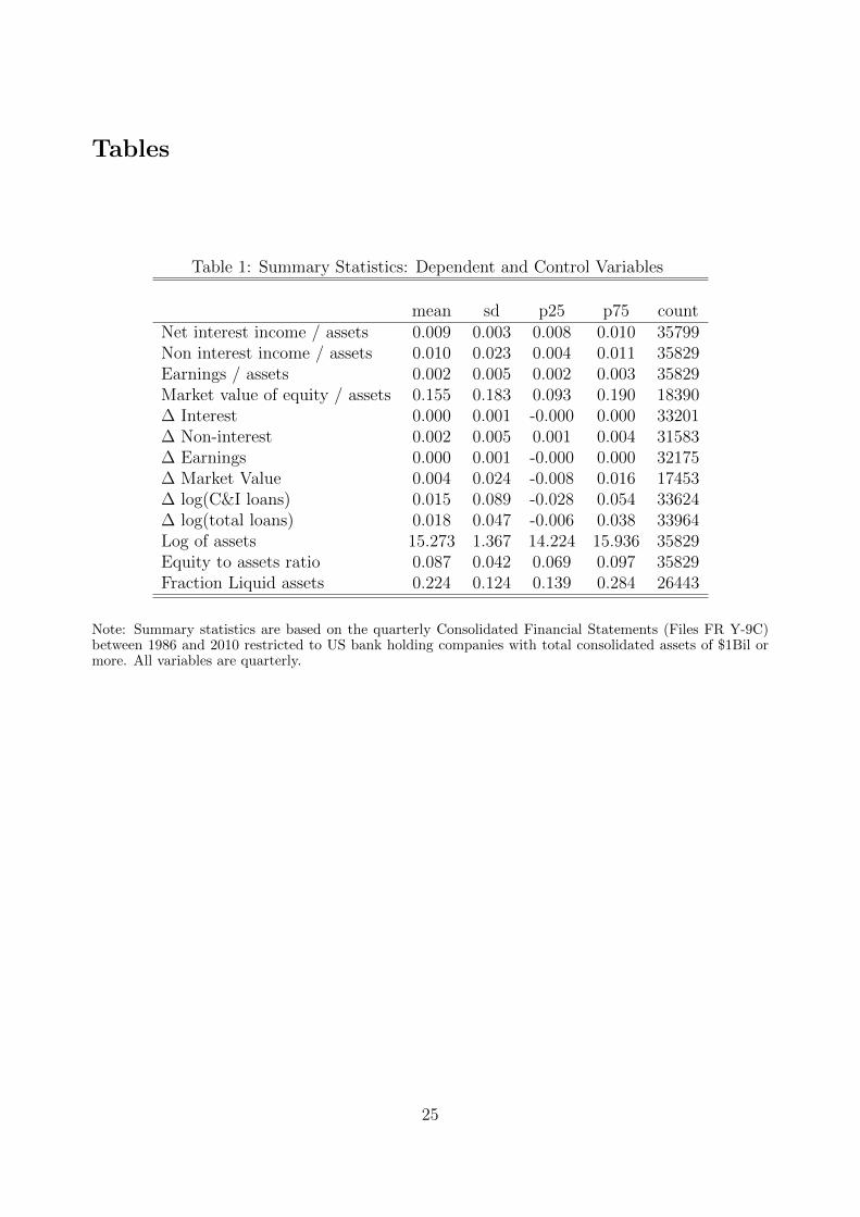
the median.1 We report summary statistics for these variables in Table 1.

There are two sets of dependent variables. First are income-related variables that we

expect should be affected by movements in interest rates: net interest income and net profits.

We also take non-interest income as a placebo variable, on which interest rates should in

principle have no impact. We normalize all these variables by total assets. Second, we

1Our results are qualitatively similar when trimming at the 5th or the 1st percentile of the distribution.

5

look at two variables measuring credit growth: the first one is the quarterly change in log

commercial and industrial loans, while the second one is the quarterly change in log total

loans.

As shown in Table 1, the quarterly change in interest income is small compared to total

assets (sample s.d. is 0.001). This is due to the fact that interest rates do not change very

much from quarter to quarter: On average, quarterly net interest income accounts for about

0.9% of total assets, while the bottomline (earnings) is less than 0.2%. Notice also that non-

interest income is as large as interest income on average (1% of assets compared to 0.9%),

but much more variable (s.d. of 0.023 vs 0.003).

Control variables are the determinants of the sensitivity of bank lending to interest rates

that have been discussed in the literature. In line with Stein and Kashyap (2000), we use

equity normalized by total assets, size (log of total assets) and the share of liquid securities.

The share of liquid securities variable differs somewhat from Kashyap and Stein’s definition

(fed funds sold + AFS securities) due to differences between BHC consolidated data and call

reports. First in our data, available-for-sale securities are only available after 1993; second,

Fed Funds sold are only available after 2001. To construct our measure of liquid securities,

we thus deviate from Kashyap and Stein’s definition and take all AFS securities normalized

by total assets. Even after this modification, our liquidity measure remains available for the

1994-2011 sub-period only.

Our control variables, obtained from accounts consolidated at the BHC-level, have orders

of magnitudes that are similar to existing studies on commercial bank-level data: Average

equity-to-asset ratio is 8.7% in our data, compared to 9.5% in Campello (2002)’s sample

(which covers the 1981-1997 period); The share of liquid assets is 27% in our sample, com-

pared to 32% in his sample. The differences naturally emanate from different sample periods

(1994-2011 vs. 1981-1997) and different measures for liquidity.2 Given these discrepancies,

the fact that both variables have similar order of magnitude is reassuring.

2Due to data availability constraints, we do not include the Fed Fund sold in our measure of liquidity.

6

2.1.2. Interest Rates

We use three time-series of interest rates. In most of our regressions, we use the fed funds

rate as our measure of short-term interest rate, available monthly from the Federal Reserve’s

website. To each quarter, we assign the value of the last month of that quarter. Second,

in Table 8, we also use a measure of long-term interest rates. We take the spread on the

10-year treasury bond, also available from the Fed’s website. Last, we construct a measure

of expected short interest rates using the citetfama87 series of zero coupon bond prices. For

each quarter t, we use as our measure of expected short rate the forward 1-year rate as of t−8

(two years before). This forward is calculated using the zero coupon bond prices according

to the formula p2,t−8/p3,t−8 − 1, where pj,s is the price of the discount bond of maturity j at

date s.

2.2. Exposure to Interest Rate Risk

2.2.1. Income Gap: Definition and Measurement

The income gap of a financial institution is defined as (see Mishkin & Eakins, 2009, chapters

17 and 23):

Income Gap = RSA− RSL (1)

where RSA are all the assets that either reprice, or mature, within one year, and RSL are all

the liabilities that mature or reprice within a year. RSA (RSL) is the number of dollars of

assets (liability) that will pay (cost) variable interest rate. Hence, income gap measures the

extent to which a bank’s net interest income are sensitive to interest rates changes. Because

the income gap is a measure of exposure to interest rate risk, Mishkin and Eakins (2009)

propose to assess the impact of a potential change in short rates ∆r on bank income by

calculating: Income Gap×∆r.

This relation has no reason to hold exactly, however. Income gap is a reasonable approx-

7

imation of a bank’s exposure to interest rate risk, but it is a noisy one. First, the cost of

debt rollover may differ from the short rate. New short-term lending/borrowing will also be

connected to the improving/worsening position of the bank on financial markets (for liabili-

ties) and on the lending market (for assets). This introduces some noise. Second, depending

on their repricing frequency, assets or liabilities that reprice may do so at moments where

short rates are not moving. This will weakens the correlation between change in interest

income and Income Gap×∆r. To see this, imagine that a bank holds a $100 loan, financed

with fixed rate debt, that reprices every year on June 1. This bank has an income gap of

$100 (RSA=100, RSL=0). Now, assume that the short rate increases by 100bp on February

20. Then, in the first quarter of the year, bank interest income is not changing at all, while

the bank has a $100 income gap and interest rates have risen by 100bp. During the second

quarter, the short rate is flat, but bank interest income is now increasing by $1 = 1%×$100.

For these two consecutive quarters, the correlation between gap-weighted rate changes and

interest income is in fact negative. Third, banks might be hedging some of their interest rate

exposure, which would weaken the link between cash flows and Income Gap×∆r. Overall,

while we expect that the income gap is connected with interest rate exposure, the relation-

ship can be quite noisy due to heterogeneity in repricing dates and repricing frequencies,

and their interaction with interest rate dynamics. The income gap is a gross approximation

of interest rate exposure; Its main advantage is that it is simple and readily available from

form FR Y-9C.

Concretely, we construct the income gap using variables from the schedule HC-H of the

form FR Y-9C, which is specifically dedicated to the interest sensitivity of the balance sheet.

RSA is directly provided (item bhck3197). RSL is decomposed into four elements: Long-

term debt that reprices within one year (item bhck3298); Long-term debt that matures

within one year (bhck3409); Variable-rate preferred stock (bhck3408); and Interest-bearing

deposit liabilities that reprice or mature within one year (bhck3296), such as certificates of

deposits. Empirically, the latter is by far the most important determinant of the liability-side

8

sensitivity to interest rates. All these items are continuously available from 1986 to 2011.

This availability is the reason why we chose to work with consolidated accounts (BHC data

instead of “Call” reports).

We scale all these variables by bank assets, and report summary statistics in Table 2.

The average income gap is 13.4% of total assets. This means that, for the average bank,

an increase in the short rate by 100bp will raise bank revenues by 0.134 percentage points

of assets. There is significant cross-sectional dispersion in income gap across banks, which

is crucial for our identification. About 78% of the observations correspond to banks with

a positive income gap: For these banks, an increase in interest rates yields an increase in

cash flows. A second salient feature of Table 2 is that RSL (interest rate-sensitive liabilities)

mostly consists of variable rate deposits, that either mature or reprice within a year. Long

term debt typically has a fixed rate.

2.2.2. Direct evidence on Interest Rate Risk Hedging

In this Section, we ask whether banks use derivatives to neutralize their “natural” exposure

to interest rate risk. We can check this directly in the data. The schedule HC-L of the form

FR Y-9C reports, starting in 2005, the notional amounts in interest derivatives contracted by

banks. Five kinds of derivative contracts are separately reported: Futures (bhck8693), For-

wards (bhck8697), Written options that are exchange traded (bhck8701), Purchased options

that are exchange traded (bhck8705), Written options traded over the counter (bhck8709),

Purchased options traded over the counter (bhck8713), and Swaps (bhck3450).

We scale all these variables by assets, and report summary statistics in Table 3. Swaps

turn out to be the most prevalent form of hedge used by banks. For the average bank, they

account for about 18% of total assets. This number, however, conceals the presence of large

outliers: a handful of banks –between 10 and 20 depending on the year– have total notional

amount of swaps greater than their assets. These banks are presumably dealers. Taking out

these outliers, the average notional amount is only 4% of total assets, a smaller number than

9

the average income gap. 40% of the observations are banks with no derivative exposure.

The data unfortunately provides us only with notional exposures. Notional amounts may

conceal offsetting positions so that the total interest rate risk exposure is minimal. To deal

with this issue, we directly look at the sensitivity of each bank’s revenue to interest rate

movement and check whether it is related to the income gap. We do this in the next Section

and find that banks revenue indeed depend on Income gap × ∆r: This confirms the direct

evidence from Table 3 that banks do not hedge out entirely their interest rate risk.

3. Interest Risk and Cash-Flows

In this Section, we check that the sensitivity of profits to interest rate movements depends

on our measure of income gap. This Section serves as a validation of our measure of income

gap, but also shows that hedging, although present in the data, is limited.

By definition (1), we know that banks profits should be directly related to Income gap×

∆r. We thus follow the specification typically used in the literature (Kashyap and Stein

(1995), Stein and Kashyap (2000); Campello (2002) for instance), and estimate the following

linear model for bank i in quarter t:

∆Yit =k=4�

k=0

αk.(gapit−1 ×∆fed fundst−k) +k=4�

k=0

γk(sizeit−1 ×∆fed fundst−k)

+k=4�

k=0

λk(equityit−1 ×∆fed fundst−k) +k=4�

k=0

θk(liquidityit−1 ×∆fed fundst−k)

+k=4�

k=0

ηk∆Yit−1−k + gapit−1 + sizeit−1 + equityit−1 + liquidityit−1 + date dummies + �it

(2)

where all variables are scaled by total assets. Yit is a measure of banks cash flows and value:

interest income, non-interest income, earnings and market value of equity (see Appendix A

for formal definitions).�k=4

k=0 αk is the cumulative effect of interest rate changes, given the

income gap of bank i. This sum is the coefficient of interest. If the income gap variable

10

contains information on bank interest rate exposure and if banks do not fully hedge this

risk, we expect�k=4

k=0 αk > 0.

Consistent with the literature, we control for existing determinants of the sensitivity of

bank behavior to interest rates: bank size (as measured through log assets) and bank equity

(equity to assets). Because of data limitation, we include bank liquidity (securities available

for sale divided by total assets) as a control only in one specification. In all regressions,

the controls are included directly and interacted with current and four lags of interest rate

changes. These controls have been shown to explain how bank lending reacts to changes in

interest rates. Their economic justification in a profit equation is less clear, but since our

ultimate goal is to explain the cross-section of bank lending, we include these controls in the

profit equations for the sake of consistency. As it turns out, their presence, or absence, does

not affect our estimates of�k=4

k=0 αk in equation (2).

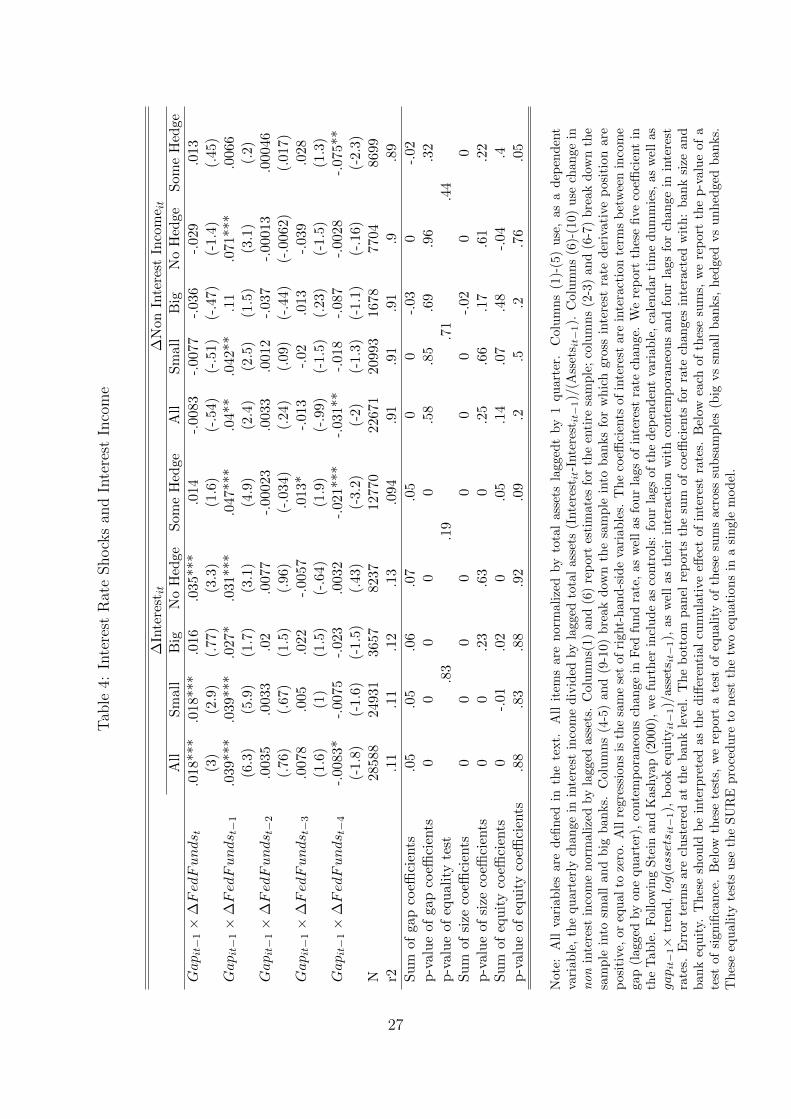
The first set of results directly looks at net interest income, which is the difference between

interest income and interest expenses. This item should be most sensitive to variations in

interests paid or received. We report the results in Table 4. Columns 1-5 use (quarterly)

changes in interest income normalized by lagged assets, as the dependent variable. Column

1 reports regression results on the whole sample. The bottom panel reports the cumulative

impact of an interest rate increase,�k=4

k=0 αk, and the p-value of the F-test of statistical

significance. For interest income, the effect of income gap weighted changes in interest rates

is strongly significant. A $1 increase in Gapit−1×∆FedFundst, after 5 consecutive quarters,

raises interest income by about 0.05 dollars. This suggests that the income gap captures

some dimension of interest rate exposure, albeit imperfectly so.

This effect applies across bank size and seems unaffected by hedging. Columns 2-3 split

the sample into large and small banks. “Large banks” are defined as the 50 largest BHCs

each quarter in terms of total assets. Both large and small banks appear to have similar

exposure to interest rate: the overall impact of interest rate changes on income (�k=4

k=0 αk)

is not statistically different across the two groups (p value = 0.83). Columns 4-5 split the

11

sample into banks that have some notional exposure on interest rate derivatives and banks

that report zero notional exposure. This sample split reduces the period of estimation to

1995-2011, as notional amounts of interest rate derivatives are not available in the data

before 1995. We find strong and statistically significant effects for both categories of banks.

While the income of banks with some derivative exposure respond slightly less to changes in

interest rate than the income of banks with no exposure, the difference is not statistically

significant (p value = .19). In non-reported regressions, we further restrict the sample to

BHCs whose notional interest rate derivative exposure exceeds 10% of total assets (some

4,000 observations): even on this smaller sample, the income gap effect remains strongly

significant and has the same order of magnitude. Overall, our results indicate that interest

rate hedging is a minor force for most banks, and even most large banks. This is consistent

with the findings reported in Begeneau et al. (2012) that the four largest US banks amplify

their balance sheet exposure with derivatives, instead of offsetting them, even partially. Their

evidence, along with ours, suggests that banks keep most interest rate risk exposure related

to lending, perhaps because hedging is too costly. This is also in line with Vickery (2008),

who shows that financial institutions alter the types of originations they do (fixed rate vs.

variable rate) depending on their ex-ante exposure to interest risk. At a broader level, this is

also consistent with Guay and Kothari (2003), who document that the impact of derivatives

on the cash-flows of non-financials is small, even in the presence of shocks to the underlying

assets.

To further validate the income gap measure, we run a “placebo test” in columns 6-10. In

these columns, we use non-interest income as a dependent variable, which includes: servicing

fees, securitization fees, management fees or trading revenue. While non-interest income may

be sensitive to interest rate fluctuations, there is no reason why this sensitivity should be

related to the income gap. Thus, with non-interest income as a dependent variable, we

expect�k=4

k=0 αk = 0 in equation (2). Columns 6-10 of Table 4 report regression estimates

of equation 2 for all banks, small banks, large banks, unhedged banks and banks with some

12

interest rate derivative notional. In all these samples, the coefficient on income gap×∆r is

small and statistically insignificant.

A natural next step is to look at the impact of the income gap on the sensitivity of overall

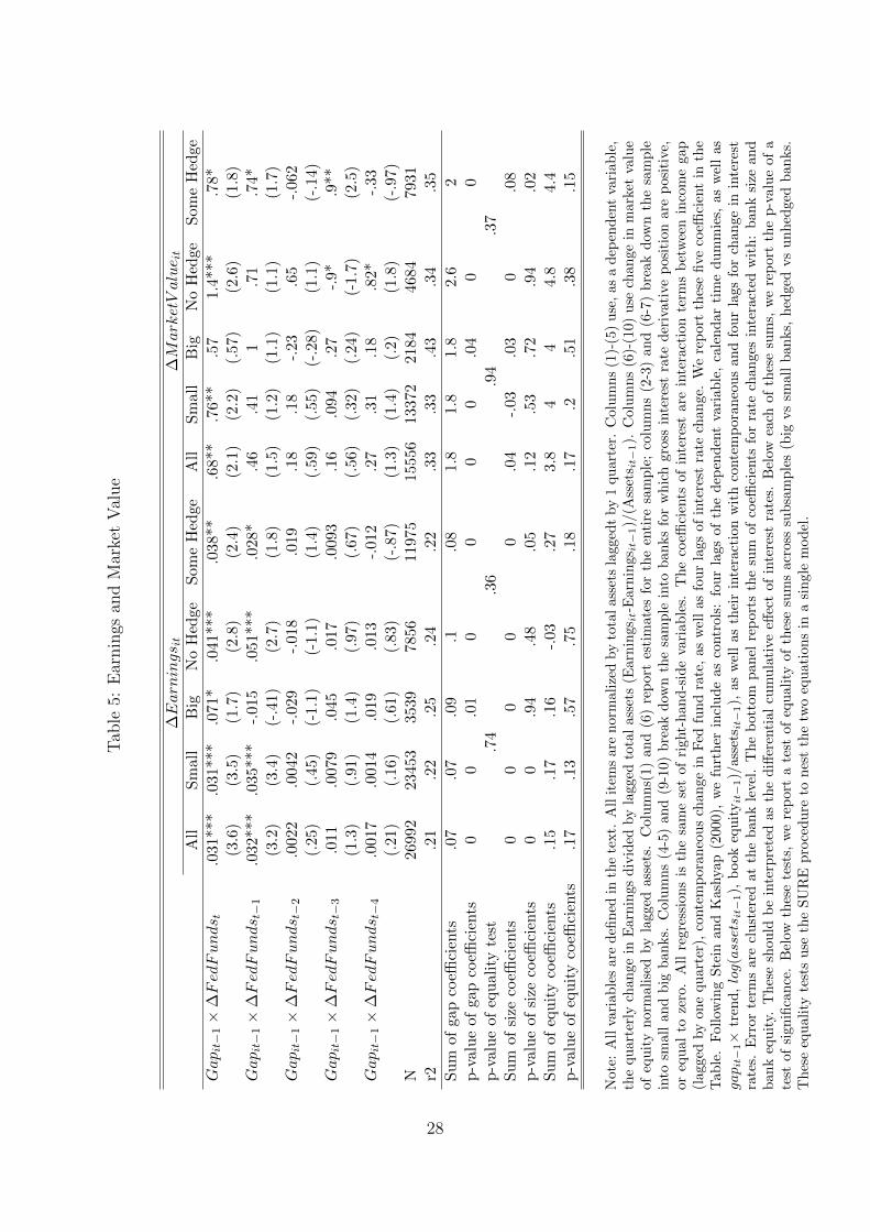
earnings and market value to changes in interest rate. We report these results in Table 5.

Columns 1-5 report the effect on earnings (of which interest income is a component), while

columns 6-10 report the effect on market value of equity. Both are normalized by total assets.�k=4

k=0 αk is positive and statistically significant at the 5% level in all our specifications. In

other words, the income gap has a significant predictive power on how banks earnings and

market value react to changes in interest rate. In column 1, the estimates show that a $1

increase in Gapit−1 × ∆FedFundst after 5 consecutive quarters raises earnings by about

$0.07. This order of magnitude is similar to the effect on interest income from Table 4. This

is not surprising since we know from Table 4, columns 6-10 that the income gap has no effect

on non-interest income. This effect remains unchanged across size groups and is not affected

by the presence of interest rate derivatives on the bank’s balance sheet (columns 2-5).

The sensitivity of banks market value to changes in interest rate also depends positively

and significantly on the income gap. The effect that we report in column 6 of Table 5

is of a similar order of magnitude than the one obtained for earnings: A $1 increase in

Gapit−1 ×∆FedFundst raises banks market value of equity by about $1.8. Given the same

shock raises earnings by $0.07, this implies an earnings multiple of approximately 25, which

is large but not unreasonable. As for earnings, the difference in the estimated effect across

size or hedging status is insignificant, even though hedged banks tend again to react less to

Gapit−1 ×∆FedFundst than banks with no interest rate derivatives.

In Appendix B, we replicate the estimation performed in Table 4 and Table 5 using an

alternative procedure also present in the literature. This alternative technique proceeds in

two steps. First, each quarter, we estimate the cross-sectional sensitivity of the dependent

variable (changes in interest income and earnings) to the income gap using linear regression.

In a second step, we regress the time series of these coefficients on changes in interests rate

13

as well as four lags of changes in interest rate. If the income gap matters, banks profits

should depend more on the income gap in the cross-section as interest rates increase. Table

B.1 shows this is the case and that estimates of�k=4

k=0 αk are similar to those obtained with

our main approach. The cumulative effect of a $1 increase in Gapit−1 ×∆FedFundst yields

a 5 cents increase in interest income and a 7 cents increase in overall earnings.

We conclude this section by emphasizing that our regressions should in principle under-

state banks exposure to interest rate risk. This is because the income gap measure we use

only gives a rough estimate of the true sensitivity of banks income to short interest move-

ments. In the absence of the full distribution of repricing dates, the one year repricing items

fail to capture important dimensions of interest rate sensitivity. Despite this caveat, the

main lessons from this Section’s analysis are that (1) our income gap measure still explains

a significant fraction of the sensitivity of bank profits to interest rate movements and (2)

this holds true even for large banks or banks with large notional amounts of interest rate

derivatives.

4. Interest Risk and Lending

4.1. Main Result

We have established that interest rate changes affect banks cash flows when the income gap

is larger. If banks are to some extent financially constrained, these cash flow shocks should

affect lending. We follow Stein and Kashyap (2000) and run the following regression:

14

∆log(creditit) =k=4�

k=0

αk.(gapit−1 ×∆fed fundst−k) +k=4�

k=0

γk(sizeit−1 ×∆fed fundst−k)

+k=4�

k=0

λk(equityit−1 ×∆fed fundst−k) +k=4�

k=0

θk(liquidityit−1 ×∆fed fundst−k)

+k=4�

k=0

ηk∆log(creditit−1−k) + gapit−1 + sizeit−1 + equityit−1 + liquidityit−1

+date dummies + �it(3)

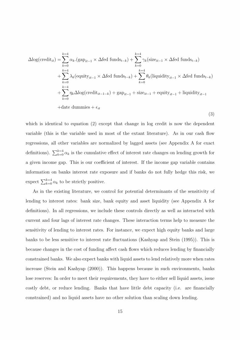
which is identical to equation (2) except that change in log credit is now the dependent

variable (this is the variable used in most of the extant literature). As in our cash flow

regressions, all other variables are normalized by lagged assets (see Appendix A for exact

definitions).�k=4

k=0 αk is the cumulative effect of interest rate changes on lending growth for

a given income gap. This is our coefficient of interest. If the income gap variable contains

information on banks interest rate exposure and if banks do not fully hedge this risk, we

expect�k=4

k=0 αk to be strictly positive.

As in the existing literature, we control for potential determinants of the sensitivity of

lending to interest rates: bank size, bank equity and asset liquidity (see Appendix A for

definitions). In all regressions, we include these controls directly as well as interacted with

current and four lags of interest rate changes. These interaction terms help to measure the

sensitivity of lending to interest rates. For instance, we expect high equity banks and large

banks to be less sensitive to interest rate fluctuations (Kashyap and Stein (1995)). This is

because changes in the cost of funding affect cash flows which reduces lending by financially

constrained banks. We also expect banks with liquid assets to lend relatively more when rates

increase (Stein and Kashyap (2000)). This happens because in such environments, banks

lose reserves: In order to meet their requirements, they have to either sell liquid assets, issue

costly debt, or reduce lending. Banks that have little debt capacity (i.e. are financially

constrained) and no liquid assets have no other solution than scaling down lending.

15

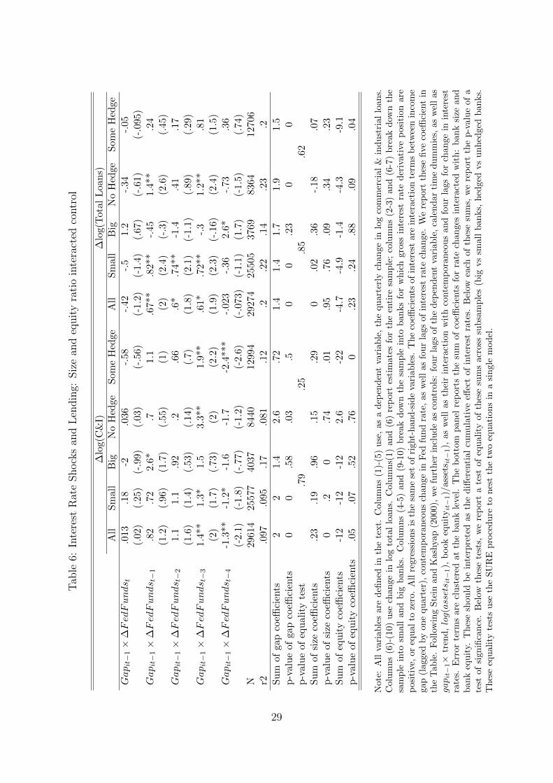
We first run regressions without the control for asset liquidity, as this variable is not

available before 1993. We report the results in Table 6: separately for C&I loan growth

(columns 1-5) and for total lending growth (columns 6-10). As before, we run regressions on

the whole sample (columns 1 and 6), split the sample into large and small banks (column 2,

3, 7 and 8) and into banks with some interest rate derivatives and banks without (column 4,

5, 9 an 10). Focusing on total lending growth, we find results that are statistically significant

at the 1% level, except for large banks. The effects are also economically significant. If we

compare a bank at the 25th percentile of the income gap distribution (approximately 0)

and a bank at the 75th percentile (approximately 0.25), and if the economy experiences an

100 basis point increase in the fed funds rate, total loans in the latter bank will grow by

about .4 percentage points more than in the former. This has to be compared with a sample

average quarterly loan growth of about 1.8%. Note also that notional holdings of interest

rate derivatives do not significantly explain cross-sectional differences in banks sensitivity

of lending growth to changes in interest rate. While the estimates of�k=4

k=0 αk drops from

1.9 to 1.5 when we move from the sample of banks with no notional exposure to interest

rate derivates to the sample of banks with a strictly positive exposure, this difference is

not statistically significant (p value = 0.62). This is consistent with the idea that banks

with notional exposure do not necessarily seek to hedge their banking book (Begeneau et

al. (2012)). We also find that the sensitivity of large banks lending growth to interest rate

changes does not depend significantly on their income gap (column 4 and 8). However, the

point estimates have the same order of magnitude for large and small banks (1.7 versus 1.4 for

total lending) and the difference between small and large banks is not statistically significant

(p value = 0.85). Finally, our results are mostly similar when using C&I loans or total loans

as dependent variables. The only difference is that the sensitivity of C&I lending growth to

changes in interest rate for banks with no notional exposure to interest rate derivatives does

not depend significantly on their income gap (column 5) while it is positive and statistically

significant when looking at total lending growth (column 10).

16

Overall, the other control variables we use to explain the sensitivity of lending growth

to changes in interest rates in a much less consistent way than our income gap measure.

In rows 4 to 6 of the bottom panel of Table 6, we report the sum of the coefficients on

interaction terms with size. Large banks decrease their lending less when the fed funds rates

increase (i.e. the coefficient is positive). On C&I loans, the estimated effect is statistically

significant (Kashyap and Stein (1995) report a similar result on commercial banks data over

the 1976-1993 period); but on total loans we find no significant impact and the coefficient is

nearly zero. The impact of size on the sensitivity of lending growth to changes in monetary

policy has the same order of magnitude as the impact of the income gap. If we compare

banks at the 25th and 75th percentile of the size distribution (log of assets equal to 14.2

vs 15.9) and consider a 100bp increase in fed funds rates, the smaller bank will reduce its

C&I lending by .3 percentage points more (compared to .4 with the income gap). Thus, the

income gap explains similar variations of C&I lending in response to monetary policy shocks

than bank size, but it explains significant variations in total lending while size does not.

Turning to the role of capitalization, rows 7 to 9 in the bottom panel of Table 6 report the

sum of the coefficients on equityit−1

assetsit−1.∆fedfundst−k. Estimates are in most cases insignificant

and have the “wrong” economic sign: better capitalized banks tend to reduce their lending

more when interest rates increase. This counterintuitive result does not come from the fact

that equity is correlated with size (negatively) or with income gap (positively): in unreported

regressions, we have tried specifications including the interactions term with equity only, and

the coefficients remained negative.

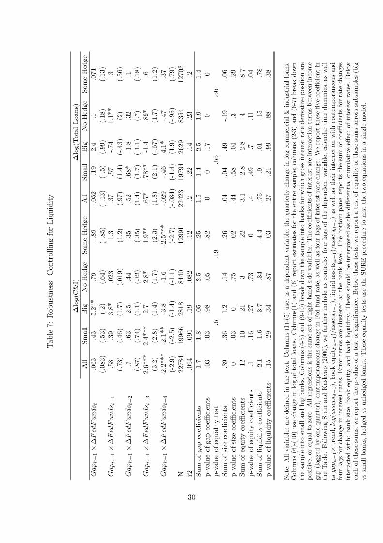
In Table 7, we include the asset liquidity control, which restricts the sample to 1993-

2011. Despite the smaller sample size, our results resist well. For C&I lending growth, they

remain statistically significant at the 5% level for all banks, small banks, and banks without

derivative exposure. For total lending growth, estimates are statistically significant at 1%

for all specification but large banks. For total lending growth, the point estimate for large

banks is similar to the estimate for small banks, but it is much less precise – a possible

17

consequence of smaller sample size. For both credit growth measures, the difference between

large and small banks is insignificant.

Asset liquidity does not, however, come in significant in these regressions, and it also

has the “wrong” economic sign: banks with more liquid assets tend to reduce their lending

more when interest rates increase, but the effect is not precisely estimated. The discrepancy

with Kashyap and Stein’s results comes from the fact that we are using BHC data, instead

of commercial bank data. BHC data report a consistent measure of income gap, while

commercial bank data fail to do so. Our use of BHC data has two consequences: First,

we work at a different level of aggregation; Most importantly, our regressions with liquidity

controls go from 1993 to 2011, while Kashyap and Stein’s sample goes from 1977 to 1993. It

is possible that reserves requirement have become less binding over the past 20 years.

In sum, we find that the income gap has significant explanatory power over the cross-

section of bank lending sensitivities to changes in interest rates. This relationship is signifi-

cant and holds more consistently across specifications than the effect of size, leverage or liquid

assets. The income gap seems to matter less for larger banks, in particular when looking at

C&I credit, consistent with the idea that larger banks are less credit constrained. Interest

derivative exposure does not appear to reduce the effect of income gap in a significant way.

5. Discussion

5.1. Credit Multiplier

This Section uses interest rate shocks to identify the credit multiplier of banks in our sample.

To do this, we reestimate a version of equation (3) where the dependent variable is defined

as quarterly increase in $ loans normalized by lagged assets. It thus differs slightly from the

measure we have been using in the previous Section (quarterly change in log loans), which

is commonly used in the literature. The advantage of this new variable is that it allows to

directly interpret the sum of the interacted coefficients�k=4

k=0 αk as the $ impact on lending

18

of a $1 increase in the interest-sensitive income, gap × ∆r. We can then directly compare

the $ impact on lending to the $ impact on cash-flows as estimated in Table 4. The ratio is

a measure of the credit multiplier.

We obtain a credit multiplier of about 11, i.e. a $1 increase in cash flows leads to an

increase in lending by $11. Using the change in $ lent normalized by total assets as the

depend variable, we find a cumulative effect of .81 (p-value = .002). This effect is strong

and statistically significant, which is not a surprise given the results of Table 6 –only the

scaling variable changes. This estimate means that a $1 increase in gap × ∆r leads to an

increase of lending by $.81. At the same time, we know from Table 4 that the same $1

increase generates an increase in total earnings of about $0.07. Hence, assuming that the

sensitivity of lending to interest rate comes only through this cash flow shock, this yields

a multiplier of 0.81/0.07=11.5. This is slightly lower than bank leverage, since the average

asset-to-equity ratio is 13.1 in our sample. Given that cash-flows are also additional reserves,

the credit multiplier we get is consistent with existing reserve requirements in the US which

are around 10 for large banks. These estimates do, however, need to be taken with caution

since lending may be affected by gap × ∆r through channels other than cash flows, as we

discuss in the next section.

5.2. Short vs long rates: Cash flow vs Collateral Channel

A potential interpretation of our results is that the income gap is a noisy measure of the

duration gap. The duration gap measures the difference of interest rate sensitivity between

the value of assets and the value of liabilities (Mishkin and Eakins (2009)). Changes in

interest rates may therefore affect the value of a bank’s equity. Changes in the value of

equity may in turn have an impact on how much future income a bank can pledge to its

investors. For a bank with a positive duration gap, an increase in interest rates raises the

value of equity and therefore its debt capacity: it can lend more. This alternative channel

also relies on a failure of the Modigliani-Miller theorem for banks, but it does not go through

19

cash flows; it goes through bank value. This is akin to a balance sheet channel, a la Bernanke

and Gertler (1989), but for banks.

Directly measuring the duration gap is difficult and would rely on strong assumptions

about the duration of assets and liabilities. Instead, to distinguish income effects and balance

sheet effects, we rely on the fact that the impact of interest rates on bank value partly comes

from long-term rates. To see this, notice that the present value at t of a safe cash-flow C

at time t + T is C(1+rt,T )T , where rt,T is the risk-free yield between t and t + T . Thus, as

long as there are shocks to long-term yields that are not proportional to shocks to short-

term yields, we can identify a balance sheet channel separately from an income channel.

Consider for instance an increase in long-term rates, keeping short-term rates constant. If

our income gap measure affects lending through shocks to asset values, we should observe

empirically that firms with lower income gap lend relatively less following this long-term

interest rates increase. By contrast, if our income gap measure affects lending only through

contemporaneous or short-term changes in income, such long-term rate shock should not

impact differently the lending of high vs. low income gap banks.

We implement this test for the presence of a balance-sheet channel in Table 8. In this

table, we simply add to our benchmark equation (3) interaction terms between the income

gap – as a proxy for the duration gap – and five lags of changes in long term interest rates,

measured as the yield on 10 years treasuries. The coefficients on these interaction terms

are reported in the lower part of the top panel. In the bottom panel, we report the sum of

these coefficients (the cumulative impact of interest rates) as well as their p-value. In this

Table, we report results for interest income, market value of equity, and the two measures

of lending growth. The sample contains all banks.

We find no evidence that long term interest rates affect bank cash flows, value or lending.

If anything, the cumulative effect goes in the opposite direction to what would be expected

if the income gap was a proxy for the duration gap. Estimates of the income gap effect are

unaffected by the inclusion of the long rate interaction terms. This test seems to suggest

20

that monetary policy affects bank lending via income gap induced cash flows shocks much

more than through shocks to the relative value of banks’ assets and liabilities. However, it is

important to emphasize that the power of test is limited by the fact that we do not directly

measure the duration gap.

5.3. Expected vs Unexpected Movements in Interest Rates

In this Section, we focus on unexpected changes in short interest rates. A possible expla-

nation for our results is that banks adapt their income gap in anticipation of short rate

movements. Well-managed banks, who anticipate a rate increase, increase their income gap

before monetary policy tightens. Then, their earnings increase mechanically with an increase

in interest rates; At the same time, their lending is less affected by the increased interest

rate, not because their earnings increase with the interest rate, but simply because they are

better managed in the first place. However, if the increase in interest rate is unexpected, this

possible explanation is less likely to hold. We thus break down variations in interest rates

into an expected and an unexpected component and perform our main regression analysis

using these two separate components.

To measure expected rate changes, we use forward short rates obtained from the Fama-

Bliss data. For the short rate in t, we take as a measure of expected rate the forward interest

rate demanded by the market at t − 2, in order to lend between t and t + 1. We then add

to our main equation (3) interaction terms between the income gap and 5 lags of changes in

expected short rates. We report regression results in Table 9 for two measures of cash-flows

and two measures of credit growth. The sample contains all banks.

Our results are mostly driven by the unexpected component of the short rate. When

controlling for the income gap interacted with expected change in the short rate, our estimate

is unchanged. The cumulative impact of the short rate change,�k=4

k=0 αk, reported in the first

line of the bottom panel of Table 9, remains statistically significant and similar in magnitude

to our previous estimations. The cumulative impact of the expected rate change, reported

21

in the third line of the bottom panel, is much smaller in magnitude and never statistically

significant (the minimum p-value being .67).

This is unsurprising given the well documented failure of the expectation hypothesis

(Fama and Bliss (1987)): even though they are the best forecast of future short rates,

forward rates have very little predictive content. In line with the existing literature, the

in-sample correlation between forward and effective short rates is .3 in levels (short rates are

persistent), but only -0.01 in quarterly changes. If banks do not have superior information

than the market, they will not be able to forecast future changes in the short rate and adapt

their income gap consequently. Results from Table 9 are consistent with this interpretation.

6. Conclusion

This paper shows that banks retain significant exposure to interest rate risk. Our sample

consists of quarterly data on US bank holding companies from 1986 to 2011. We measure

interest-sensitivity of profit through the income gap, defined as the difference between assets

and liabilities that mature in less than one year. The average income gap in our sample is

13.5% of total assets, but it exhibits significant cross-sectional variation. The income gap

strongly predicts how bank profits will react to future movements in interest rates.

We also find that banks exposure to interest rate risk has implications for the transmission

of monetary policy. When the Federal Reserve increases short rates, this affects bank cash

flows and hence their lending policy. In other words, the income gap has a strong explanatory

power on the sensitivity of lending to changes in interest rates. This variable has a stronger,

more consistent impact than previously identified factors, such as leverage, bank size or even

asset liquidity. Finally, we report evidence consistent with the hypothesis that our main

channel is a cash-flow effect, as opposed to a collateral channel: Interest rates affect lending

because they affect cash flows, not because they affect the market value of equity.

Our results suggest that the allocation of interest rate exposure across agents (banks,

22

households, firms, government) may explain how an economy responds to monetary policy.

In particular, the distribution of interest rate risk across agents is crucial to understand the

redistributive effects of monetary policy and thus to trace the roots of the transmission of

monetary policy.

References

Adrian, Tobias and Hyun Song Shin, “Liquidity and leverage,” Journal of Financial

Intermediation, July 2010, 19 (3), 418–437.

Begeneau, Juliane, Monika Piazzesi, and Martin Schneider, “The Allocation of

Interest Rate Risk in the Financial Sector,” Working Paper, Stanford University 2012.

Bernanke, Ben and Mark Gertler, “Agency Costs, Net Worth, and Business Fluctua-

tions,” American Economic Review, March 1989, 79 (1), 14–31.

Campello, Murillo, “Internal Capital Markets in Financial Conglomerates: Evidence from

Small Bank Responses to Monetary Policy,” Journal of Finance, December 2002, 57 (6),

2773–2805.

Chava, Sudheer and Amiyatosh Purnanandam, “Determinants of the floating-to-fixed

rate debt structure of firms,” Journal of Financial Economics, September 2007, 85 (3),

755–786.

Fama, Eugene F and Robert R Bliss, “The Information in Long-Maturity Forward

Rates,” American Economic Review, September 1987, 77 (4), 680–92.

Flannery, Mark J and Christopher M James, “The Effect of Interest Rate Changes

on the Common Stock Returns of Financial Institutions,” Journal of Finance, September

1984, 39 (4), 1141–53.

23

Gambacorta, Leonardo and Paolo Emilio Mistrulli, “Does bank capital affect lending

behavior?,” Journal of Financial Intermediation, October 2004, 13 (4), 436–457.

Guay, Wayne and S. P Kothari, “How much do firms hedge with derivatives?,” Journal

of Financial Economics, December 2003, 70 (3), 423–461.

Kashyap, Anil K. and Jeremy C. Stein, “The impact of monetary policy on bank

balance sheets,” Carnegie-Rochester Conference Series on Public Policy, June 1995, 42

(1), 151–195.

Kishan, Ruby P and Timothy P Opiela, “Bank Size, Bank Capital, and the Bank

Lending Channel,” Journal of Money, Credit and Banking, February 2000, 32 (1), 121–41.

Mishkin, Frederic and Stanly Eakins, Financial Markets and Institutions, 6 ed., Pearson

Prentice Hall, 2009.

Purnanandam, Amiyatosh, “Interest rate derivatives at commercial banks: An empirical

investigation,” Journal of Monetary Economics, September 2007, 54 (6), 1769–1808.

Stein, Jeremy C. and Anil K. Kashyap, “What Do a Million Observations on Banks Say

about the Transmission of Monetary Policy?,” American Economic Review, June 2000, 90

(3), 407–428.

Vickery, James, “How do financial frictions shape the product market? evidence from

mortgage originations,” Technical Report, Federal Reserve Bank of New York 2008.

24

Tables

Table 1: Summary Statistics: Dependent and Control Variables

mean sd p25 p75 countNet interest income / assets 0.009 0.003 0.008 0.010 35799Non interest income / assets 0.010 0.023 0.004 0.011 35829Earnings / assets 0.002 0.005 0.002 0.003 35829Market value of equity / assets 0.155 0.183 0.093 0.190 18390∆ Interest 0.000 0.001 -0.000 0.000 33201∆ Non-interest 0.002 0.005 0.001 0.004 31583∆ Earnings 0.000 0.001 -0.000 0.000 32175∆ Market Value 0.004 0.024 -0.008 0.016 17453∆ log(C&I loans) 0.015 0.089 -0.028 0.054 33624∆ log(total loans) 0.018 0.047 -0.006 0.038 33964Log of assets 15.273 1.367 14.224 15.936 35829Equity to assets ratio 0.087 0.042 0.069 0.097 35829Fraction Liquid assets 0.224 0.124 0.139 0.284 26443

Note: Summary statistics are based on the quarterly Consolidated Financial Statements (Files FR Y-9C)between 1986 and 2010 restricted to US bank holding companies with total consolidated assets of $1Bil ormore. All variables are quarterly.

25

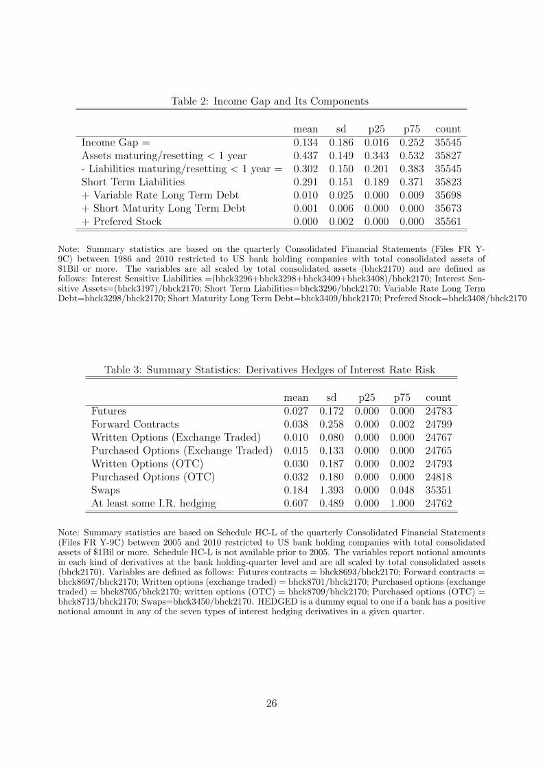
Table 2: Income Gap and Its Components

mean sd p25 p75 countIncome Gap = 0.134 0.186 0.016 0.252 35545Assets maturing/resetting < 1 year 0.437 0.149 0.343 0.532 35827- Liabilities maturing/resetting < 1 year = 0.302 0.150 0.201 0.383 35545Short Term Liabilities 0.291 0.151 0.189 0.371 35823+ Variable Rate Long Term Debt 0.010 0.025 0.000 0.009 35698+ Short Maturity Long Term Debt 0.001 0.006 0.000 0.000 35673+ Prefered Stock 0.000 0.002 0.000 0.000 35561

Note: Summary statistics are based on the quarterly Consolidated Financial Statements (Files FR Y-9C) between 1986 and 2010 restricted to US bank holding companies with total consolidated assets of$1Bil or more. The variables are all scaled by total consolidated assets (bhck2170) and are defined asfollows: Interest Sensitive Liabilities =(bhck3296+bhck3298+bhck3409+bhck3408)/bhck2170; Interest Sen-sitive Assets=(bhck3197)/bhck2170; Short Term Liabilities=bhck3296/bhck2170; Variable Rate Long TermDebt=bhck3298/bhck2170; Short Maturity Long Term Debt=bhck3409/bhck2170; Prefered Stock=bhck3408/bhck2170

Table 3: Summary Statistics: Derivatives Hedges of Interest Rate Risk

mean sd p25 p75 countFutures 0.027 0.172 0.000 0.000 24783Forward Contracts 0.038 0.258 0.000 0.002 24799Written Options (Exchange Traded) 0.010 0.080 0.000 0.000 24767Purchased Options (Exchange Traded) 0.015 0.133 0.000 0.000 24765Written Options (OTC) 0.030 0.187 0.000 0.002 24793Purchased Options (OTC) 0.032 0.180 0.000 0.000 24818Swaps 0.184 1.393 0.000 0.048 35351At least some I.R. hedging 0.607 0.489 0.000 1.000 24762

Note: Summary statistics are based on Schedule HC-L of the quarterly Consolidated Financial Statements(Files FR Y-9C) between 2005 and 2010 restricted to US bank holding companies with total consolidatedassets of $1Bil or more. Schedule HC-L is not available prior to 2005. The variables report notional amountsin each kind of derivatives at the bank holding-quarter level and are all scaled by total consolidated assets(bhck2170). Variables are defined as follows: Futures contracts = bhck8693/bhck2170; Forward contracts =bhck8697/bhck2170; Written options (exchange traded) = bhck8701/bhck2170; Purchased options (exchangetraded) = bhck8705/bhck2170; written options (OTC) = bhck8709/bhck2170; Purchased options (OTC) =bhck8713/bhck2170; Swaps=bhck3450/bhck2170. HEDGED is a dummy equal to one if a bank has a positivenotional amount in any of the seven types of interest hedging derivatives in a given quarter.

26

Tab

le4:

Interest

RateShocks

andInterest

Income

∆Interest

it∆Non

Interest

Income it

All

Small

Big

NoHed

geSom

eHed

geAll

Small

Big

NoHed

geSom

eHed

geGap

it−1×

∆FedFunds

t.018

***

.018

***

.016

.035

***

.014

-.00

83-.00

77-.03

6-.02

9.013

(3)

(2.9)

(.77

)(3.3)

(1.6)

(-.54)

(-.51)

(-.47)

(-1.4)

(.45

)Gap

it−1×

∆FedFunds

t−1

.039

***

.039

***

.027

*.031

***

.047

***

.04*

*.042

**.11

.071

***

.006

6(6.3)

(5.9)

(1.7)

(3.1)

(4.9)

(2.4)

(2.5)

(1.5)

(3.1)

(.2)

Gap

it−1×

∆FedFunds

t−2

.003

5.003

3.02

.007

7-.00

023

.003

3.001

2-.03

7-.00

013

.000

46(.76

)(.67

)(1.5)

(.96

)(-.034

)(.24

)(.09

)(-.44)

(-.006

2)(.01

7)Gap

it−1×

∆FedFunds

t−3

.007

8.005

.022

-.00

57.013

*-.01

3-.02

.013

-.03

9.028

(1.6)

(1)

(1.5)

(-.64)

(1.9)

(-.99)

(-1.5)

(.23

)(-1.5)

(1.3)

Gap

it−1×

∆FedFunds

t−4

-.00

83*

-.00

75-.02

3.003

2-.02

1***

-.03

1**

-.01

8-.08

7-.00

28-.07

5**

(-1.8)

(-1.6)

(-1.5)

(.43

)(-3.2)

(-2)

(-1.3)

(-1.1)

(-.16)

(-2.3)

N28

588

2493

136

5782

3712

770

2267

120

993

1678

7704

8699

r2.11

.11

.12

.13

.094

.91

.91

.91

.9.89

Sum

ofga

pcoeffi

cients

.05

.05

.06

.07

.05

00

-.03

0-.02

p-valueof

gapcoeffi

cients

00

00

0.58

.85

.69

.96

.32

p-valueof

equalitytest

.83

.19

.71

.44

Sum

ofsize

coeffi

cients

00

00

00

0-.02

00

p-valueof

size

coeffi

cients

00

.23

.63

0.25

.66

.17

.61

.22

Sum

ofequitycoeffi

cients

0-.01

.02

0.05

.14

.07

.48

-.04

.4p-valueof

equitycoeffi

cients

.88

.83

.88

.92

.09

.2.5

.2.76

.05

Note:

Allvariab

lesaredefined

inthetext.Allitem

sarenormalized

bytotalassets

laggedtby

1qu

arter.

Columns(1)-(5)use,as

adep

endent

variab

le,thequ

arterlychan

gein

interest

incomedivided

bylagged

totalassets

(Interest it-Interest

it−1)/(A

ssets it−

1).

Columns(6)-(10)

use

chan

gein

non

interest

incomenormalized

bylagged

assets.Columns(1)

and(6)reportestimates

fortheentire

sample;columns(2-3)an

d(6-7)break

dow

nthe

sample

into

smallan

dbig

ban

ks.Columns(4-5)an

d(9-10)

break

dow

nthesample

into

ban

ksforwhichgrossinterest

rate

derivativepositionare

positive,

orequal

tozero.Allregression

sisthesamesetof

righ

t-han

d-sidevariab

les.

Thecoeffi

cients

ofinterest

areinteractionterm

sbetweenincome

gap(laggedby

onequ

arter),contem

poran

eouschan

gein

Fed

fundrate,as

wellas

fourlags

ofinterest

rate

chan

ge.Wereportthesefive

coeffi

cientin

theTab

le.FollowingStein

andKashy

ap(2000),wefurther

includeas

controls:fourlags

ofthedep

endentvariab

le,calendar

timedummies,as

wellas

gap i

t−1×

tren

d,log(assets

it−1),

boo

kequity i

t−1)/assets

it−1),

aswellas

theirinteractionwithcontem

poran

eousan

dfourlags

forchan

gein

interest

rates.

Error

term

sareclustered

attheban

klevel.

Thebottom

pan

elreports

thesum

ofcoeffi

cients

forrate

chan

gesinteracted

with:ban

ksize

and

ban

kequity.

Theseshou

ldbeinterpretedas

thedifferential

cumulative

effectof

interest

rates.

Below

each

ofthesesums,

wereportthep-valueof

atest

ofsign

ificance.Below

thesetests,

wereportatest

ofequalityof

thesesumsacross

subsamples(big

vssm

allban

ks,hedgedvs

unhedgedban

ks.

Theseequalitytestsuse

theSURE

procedure

tonestthetw

oequationsin

asinglemod

el.

27

Tab

le5:

Earnings

andMarketValue

∆Ear

nings

it∆M

arketValue it

All

Small

Big

NoHed

geSom

eHed

geAll

Small

Big

NoHed

geSom

eHed

geGap

it−1×

∆FedFunds

t.031

***

.031

***

.071

*.041

***

.038

**.68*

*.76*

*.57

1.4*

**.78*

(3.6)

(3.5)

(1.7)

(2.8)

(2.4)

(2.1)

(2.2)

(.57

)(2.6)

(1.8)

Gap

it−1×

∆FedFunds

t−1

.032

***

.035

***

-.01

5.051

***

.028

*.46

.41

1.71

.74*

(3.2)

(3.4)

(-.41)

(2.7)

(1.8)

(1.5)

(1.2)

(1.1)

(1.1)

(1.7)

Gap

it−1×

∆FedFunds

t−2

.002

2.004

2-.02

9-.01

8.019

.18

.18

-.23

.65

-.06

2(.25

)(.45

)(-1.1)

(-1.1)

(1.4)

(.59

)(.55

)(-.28)

(1.1)

(-.14)

Gap

it−1×

∆FedFunds

t−3

.011

.007

9.045

.017

.009

3.16

.094

.27

-.9*

.9**

(1.3)

(.91

)(1.4)

(.97

)(.67

)(.56

)(.32

)(.24

)(-1.7)

(2.5)

Gap

it−1×

∆FedFunds

t−4

.001

7.001

4.019

.013

-.01

2.27

.31

.18

.82*

-.33

(.21

)(.16

)(.61

)(.83

)(-.87)

(1.3)

(1.4)

(.2)

(1.8)

(-.97)

N26

992

2345

335

3978

5611

975

1555

613

372

2184

4684

7931

r2.21

.22

.25

.24

.22

.33

.33

.43

.34

.35

Sum

ofga

pcoeffi

cients

.07

.07

.09

.1.08

1.8

1.8

1.8

2.6

2p-valueof

gapcoeffi

cients

00

.01

00

00

.04

00

p-valueof

equalitytest

.74

.36

.94

.37

Sum

ofsize

coeffi

cients

00

00

0.04

-.03

.03

0.08

p-valueof

size

coeffi

cients

00

.94

.48

.05

.12

.53

.72

.94

.02

Sum

ofequitycoeffi

cients

.15

.17

.16

-.03

.27

3.8

44

4.8

4.4

p-valueof

equitycoeffi

cients

.17

.13

.57

.75

.18

.17

.2.51

.38

.15

Note:

Allvariab

lesaredefined

inthetext.Allitem

sarenormalized

bytotalassets

laggedtby

1qu

arter.

Columns(1)-(5)use,as

adep

endentvariab

le,

thequ

arterlychan

gein

Earnings

divided

bylagged

totalassets

(Earnings

it-E

arnings

it−1)/(A

ssets it−

1).

Columns(6)-(10)

use

chan

gein

marketvalue

ofequitynormalised

bylagged

assets.Columns(1)

and(6)reportestimates

fortheentire

sample;columns(2-3)an

d(6-7)break

dow

nthesample

into

smallan

dbig

ban

ks.Columns(4-5)an

d(9-10)

break

dow

nthesample

into

ban

ksforwhichgrossinterest

rate

derivativepositionarepositive,

orequal

tozero.Allregression

sis

thesamesetof

righ

t-han

d-sidevariab

les.

Thecoeffi

cients

ofinterest

areinteractionterm

sbetweenincomegap

(laggedby

onequ

arter),contem

poran

eouschan

gein

Fed

fundrate,as

wellas

fourlags

ofinterest

rate

chan

ge.Wereportthesefive

coeffi

cientin

the

Tab

le.FollowingStein

andKashy

ap(2000),wefurther

includeas

controls:fourlags

ofthedep

endentvariab

le,calendar

timedummies,

aswellas

gap i

t−1×

tren

d,log(assets

it−1),

boo

kequity i

t−1)/assets

it−1),

aswellas

theirinteractionwithcontem

poran

eousan

dfourlags

forchan

gein

interest

rates.

Error

term

sareclustered

attheban

klevel.

Thebottom

pan

elreports

thesum

ofcoeffi

cients

forrate

chan

gesinteracted

with:ban

ksize

and

ban

kequity.

Theseshou

ldbeinterpretedas

thedifferential

cumulative

effectof

interest

rates.

Below

each

ofthesesums,

wereportthep-valueof

atest

ofsign

ificance.Below

thesetests,

wereportatest

ofequalityof

thesesumsacross

subsamples(big

vssm

allban

ks,hedgedvs

unhedgedban

ks.

Theseequalitytestsuse

theSURE

procedure

tonestthetw

oequationsin

asinglemod

el.

28

Tab

le6:

Interest

RateShocks

andLending:

Sizean

dequityratiointeracted

control

∆log(C&I)

∆log(Total

Loa

ns)

All

Small

Big

NoHed

geSom

eHed

geAll

Small

Big

NoHed

geSom

eHed

geGap

it−1×

∆FedFunds

t.013

.18

-2.036

-.58

-.42

-.5

1.2

-.34

-.05

(.02

)(.25

)(-.99)

(.03

)(-.56)

(-1.2)

(-1.4)

(.67

)(-.61)

(-.095

)Gap

it−1×

∆FedFunds

t−1

.82

.72

2.6*

.71.1

.67*

*.82*

*-.45

1.4*

*.24

(1.2)

(.96

)(1.7)

(.55

)(1)

(2)

(2.4)

(-.3)

(2.6)

(.45

)Gap

it−1×

∆FedFunds

t−2

1.1

1.1

.92

.2.66

.6*

.74*

*-1.4

.41

.17

(1.6)

(1.4)

(.53

)(.14

)(.7)

(1.8)

(2.1)

(-1.1)

(.89

)(.29

)Gap

it−1×

∆FedFunds

t−3

1.4*

*1.3*

1.5

3.3*

*1.9*

*.61*

.72*

*-.3

1.2*

*.81

(2)

(1.7)

(.73

)(2)

(2.2)

(1.9)

(2.3)

(-.16)

(2.4)

(1.5)

Gap

it−1×

∆FedFunds

t−4

-1.3**

-1.2*

-1.6

-1.7

-2.4**

*-.02

3-.36

2.6*

-.73

.36

(-2.1)

(-1.8)

(-.77)

(-1.2)

(-2.6)

(-.073

)(-1.1)

(1.7)

(-1.5)

(.74

)N

2961

425

577

4037

8440

1299

429

274

2550

537

6983

6412

706

r2.097

.095

.17

.081

.12

.2.22

.14

.23

.2Sum

ofga

pcoeffi

cients

22

1.4

2.6

.72

1.4

1.4

1.7

1.9

1.5

p-valueof

gapcoeffi

cients

00

.58

.03

.50

0.23

00

p-valueof

equalitytest

.79

.25

.85

.62

Sum

ofsize

coeffi

cients

.23

.19

.96

.15

.29

0.02

.36

-.18

.07

p-valueof

size

coeffi

cients

0.2

0.74

.01

.95

.76

.09

.34

.23

Sum

ofequitycoeffi

cients

-12

-12

-12

2.6

-22

-4.7

-4.9

-1.4

-4.3

-9.1

p-valueof

equitycoeffi

cients

.05

.07

.52

.76

0.23

.24

.88

.09

.04

Note:

Allvariab

lesaredefined

inthetext.Columns(1)-(5)use,as

adep

endentvariab

le,thequ

arterlychan

gein

logcommercial

&industrial

loan

s.Columns(6)-(10)

use

chan

gein

logtotalloan

s.Columns(1)

and(6)reportestimates

fortheentire

sample;columns(2-3)an

d(6-7)break

dow

nthe

sample

into

smallan

dbig

ban

ks.Columns(4-5)an

d(9-10)

break

dow

nthesample

into

ban

ksforwhichgrossinterest

rate

derivativepositionare

positive,

orequal

tozero.Allregression

sisthesamesetof

righ

t-han

d-sidevariab

les.

Thecoeffi

cients

ofinterest

areinteractionterm

sbetweenincome

gap(laggedby

onequ

arter),contem

poran

eouschan

gein

Fed

fundrate,as

wellas

fourlags

ofinterest

rate

chan

ge.Wereportthesefive

coeffi

cientin

theTab

le.FollowingStein

andKashy

ap(2000),wefurther

includeas

controls:fourlags

ofthedep

endentvariab

le,calendar

timedummies,as

wellas

gap i

t−1×

tren

d,log(assets

it−1),

boo

kequity i

t−1)/assets

it−1),

aswellas

theirinteractionwithcontem

poran

eousan

dfourlags

forchan

gein

interest

rates.

Error

term

sareclustered

attheban

klevel.

Thebottom

pan

elreports

thesum

ofcoeffi

cients

forrate

chan

gesinteracted

with:ban

ksize

and

ban

kequity.

Theseshou

ldbeinterpretedas

thedifferential

cumulative

effectof

interest

rates.

Below

each

ofthesesums,

wereportthep-valueof

atest

ofsign

ificance.Below

thesetests,

wereportatest

ofequalityof

thesesumsacross

subsamples(big

vssm

allban

ks,hedgedvs

unhedgedban

ks.

Theseequalitytestsuse

theSURE

procedure

tonestthetw

oequationsin

asinglemod

el.

29

Tab

le7:

Rob

ustness:

Con

trollingforLiquidity

∆log(C&I)

∆log(Total

Loa

ns)

All

Small

Big

NoHed

geSom

eHed

geAll

Small

Big

NoHed

geSom

eHed

geGap

it−1×

∆FedFunds

t.063

.43

-5.2**

.79

-.89

-.05

2-.19

2.4

.1.071

(.08

3)(.53

)(-2)

(.64

)(-.85)

(-.13)

(-.5)

(.99

)(.18

)(.13

)Gap

it−1×

∆FedFunds

t−1

.58

.39

3.8*

.023

1.3

.37

.57

-.74

1.1*

*.3

(.73

)(.46

)(1.7)

(.01

9)(1.2)

(.97

)(1.4)

(-.43)

(2)

(.56

)Gap

it−1×

∆FedFunds

t−2

.7.63

2.5

.44

.35

.52

.68*

-1.8

.32

.1(.87

)(.74

)(1.1)

(.32

)(.35

)(1.4)

(1.7)

(-1.1)

(.7)

(.18

)Gap

it−1×

∆FedFunds

t−3

2.6*

**2.4*

**2.7

2.8*

1.9*

*.67*

.78*

*-1.4

.89*

.6(3.2)

(2.8)

(1.4)

(1.7)

(2.3)

(1.8)

(2.1)

(-.67)

(1.7)

(1.2)

Gap

it−1×

∆FedFunds

t−4

-2.2**

*-2.1**

-3.8

-1.6

-2.5**

*-.02

9-.46

4.1*

-.47

.37

(-2.9)

(-2.5)

(-1.4)

(-1.1)

(-2.7)

(-.084

)(-1.4)

(1.9)

(-.95)

(.79

)N

2278

419

966

2818

8440

1299

122

423

1979

426

2983

6412

703

r2.094

.091

.19

.082

.12

.2.22

.14

.23

.2Sum

ofga

pcoeffi

cients

1.7

1.8

.05

2.5

.25

1.5

1.4

2.5

1.9

1.4

p-valueof

gapcoeffi

cients

.03

.03

.98

.05

.82

00

.17

00

p-valueof

equalitytest

.6.19

.55

.56

Sum

ofsize

coeffi

cients

.39

.36

1.2

.14

.26

.04

.04

.49

-.19

.06

p-valueof

size

coeffi

cients

0.03

0.75

.02

.44

.58

.04

.3.29

Sum

ofequitycoeffi

cients

-12

-10

-21

3-22

-3.1

-2.8

-2.8

-4-8.7

p-valueof

equitycoeffi

cients

.1.16

.27

.73

0.4

.49

.7.11

.04

Sum

ofliqu

iditycoeffi

cients

-2.1

-1.6

-3.7

-.34

-4.4

-.75

-.9

.01

-.15

-.78

p-valueof

liqu

iditycoeffi

cients

.15

.29

.34

.87

.03

.27

.21

.99

.88

.38

Note:

Allvariab

lesaredefined

inthetext.Columns(1)-(5)use,as

adep

endentvariab

le,thequ

arterlychan

gein

logcommercial

&industrial

loan

s.Columns(6)-(10)

use

chan

gein

logof

totalloan

s.Columns(1)

and(6)reportestimates

fortheentire

sample;columns(2-3)an

d(6-7)break

dow

nthesample

into

smallan

dbig

ban

ks.Columns(4-5)an

d(9-10)

break

dow

nthesample

into

ban

ksforwhichgrossinterest

rate

derivativepositionare

positive,

orequal

tozero.Allregression

sisthesamesetof

righ

t-han

d-sidevariab

les.

Thecoeffi

cients

ofinterest

areinteractionterm

sbetweenincome

gap(laggedby

onequ

arter),contem

poran

eouschan

gein

Fed

fundrate,as

wellas

fourlags

ofinterest

rate

chan

ge.Wereportthesefive

coeffi

cientin

theTab

le.FollowingStein

andKashy

ap(2000),wefurther

includeas

controls:fourlags

ofthedep

endentvariab

le,calendar

timedummies,

aswell

asga

p it−

1×

tren

d,log(assets

it−1),

boo

kequity i

t−1)/assets

it−1),

liqu

idassets

it−1)/assets

it−1)as

wellas

theirinteractionwithcontem

poran

eousan

dfourlags

forchan

gein

interest

rates.

Error

term

sareclustered

attheban

klevel.

Thebottom

pan

elreports

thesum

ofcoeffi

cients

forrate

chan

ges

interacted

with:ban

ksize,ban

kequity,

andban

kliqu

idity.

Theseshou

ldbeinterpretedas

thedifferential

cumulative

effectof

interest

rates.

Below

each

ofthesesums,wereportthep-valueof

atest

ofsign

ificance.Below

thesetests,wereportatest

ofequalityof

thesesumsacross

subsamples(big

vssm

allban

ks,hedgedvs

unhedgedban

ks.Theseequalitytestsuse

theSURE

procedure

tonestthetw

oequationsin

asinglemod

el.

30

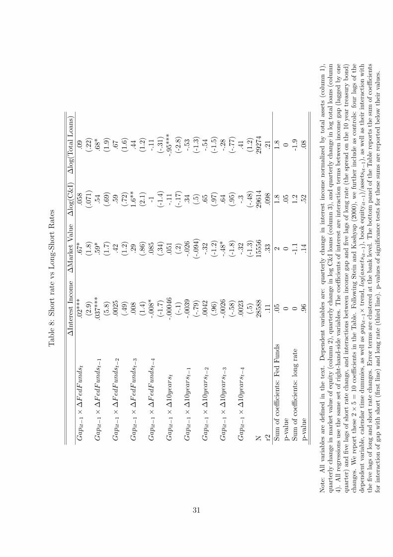
Tab

le8:

Shortrate

vsLon

g-ShortRates

∆Interest

Income

∆MarketValue

∆log(C&I)

∆log(Total

Loa

ns)

Gap

it−1×

∆FedFunds

t.02*

**.67*

.058

.09

(2.9)

(1.8)

(.07

1)(.22

)Gap

it−1×

∆FedFunds

t−1

.037

***

.59*

.54

.68*

(5.8)

(1.7)

(.69

)(1.9)

Gap

it−1×

∆FedFunds

t−2

.002

5.42

.59

.67

(.49

)(1.2)

(.72

)(1.6)

Gap

it−1×

∆FedFunds

t−3

.008

.29

1.6*

*.44

(1.4)

(.86

)(2.1)

(1.2)

Gap

it−1×

∆FedFunds

t−4

-.00

8*.085

-1-.11

(-1.7)

(.34

)(-1.4)

(-.31)

Gap

it−1×

∆10

year

s t-.00

046

.051

-.11

-.95

***

(-.1)

(.2)

(-.17)

(-2.8)

Gap

it−1×

∆10

year

s t−1

-.00

39-.02

6.34

-.53

(-.79)

(-.094

)(.5)

(-1.3)

Gap

it−1×

∆10

year

s t−2

.004

2-.32

.65

-.54

(.96

)(-1.2)

(.97

)(-1.5)

Gap

it−1×

∆10

year

s t−3

-.00

26-.48

*.64

-.28

(-.58)

(-1.8)

(.95

)(-.77)

Gap

it−1×

∆10

year

s t−4

.002

3-.32

-.3

.41

(.5)

(-1.3)

(-.48)

(1.2)

N28

588

1555

629

614

2927

4r2

.11

.33

.098

.21

Sum

ofcoeffi

cients:Fed

Funds

.05

21.8

1.8

p-value

00

.05

0Sum

ofcoeffi

cients:longrate

0-1.1

1.2

-1.9

p-value

.96

.14

.52

.08

Note:

Allvariab

lesaredefined

inthetext.Dep

endentvariab

lesare:

quarterlychan

gein

interest

incomenormalized

bytotalassets

(column1),

quarterlychan

gein

marketvalueof

equity(column2),qu

arterlychan

gein

logC&Iloan

s(column3),an

dqu

arterlychan

gein

logtotalloan

s(column

4).Allregression

suse

thesamesetof

righ

t-han

d-sidevariab

les.

Thecoeffi

cients

ofinterest

areinteractionterm

sbetweenincomegap(laggedby

one

quarter)

andfive

lags

ofshortrate

chan

ge,an

dinteractionsbetweenincomegapan

dfive

lags

oflongrate

(thespread

onthe10

year

treasury

bon

d)

chan

ges.

Wereportthese2×

5=

10coeffi

cients

intheTab

le.FollowingStein

andKashy

ap(2000),wefurther

includeas

controls:fourlags

ofthe

dep

endentvariab

le,calendar

timedummies,as

wellas

gap i

t−1×

tren

d,log(assets

it−1),boo

kequity i

t−1)/assets

it−1),as

wellas

theirinteractionwith

thefive

lags

oflongan

dshortrate

chan

ges.

Error

term

sareclustered

attheban

klevel.Thebottom

pan

elof

theTab

lereports

thesum

ofcoeffi

cients

forinteractionof

gapwithshort(firstline)

andlongrate

(thirdline).p-values

ofsign

ificance

testsforthesesumsarereportedbelow

theirvalues.

31

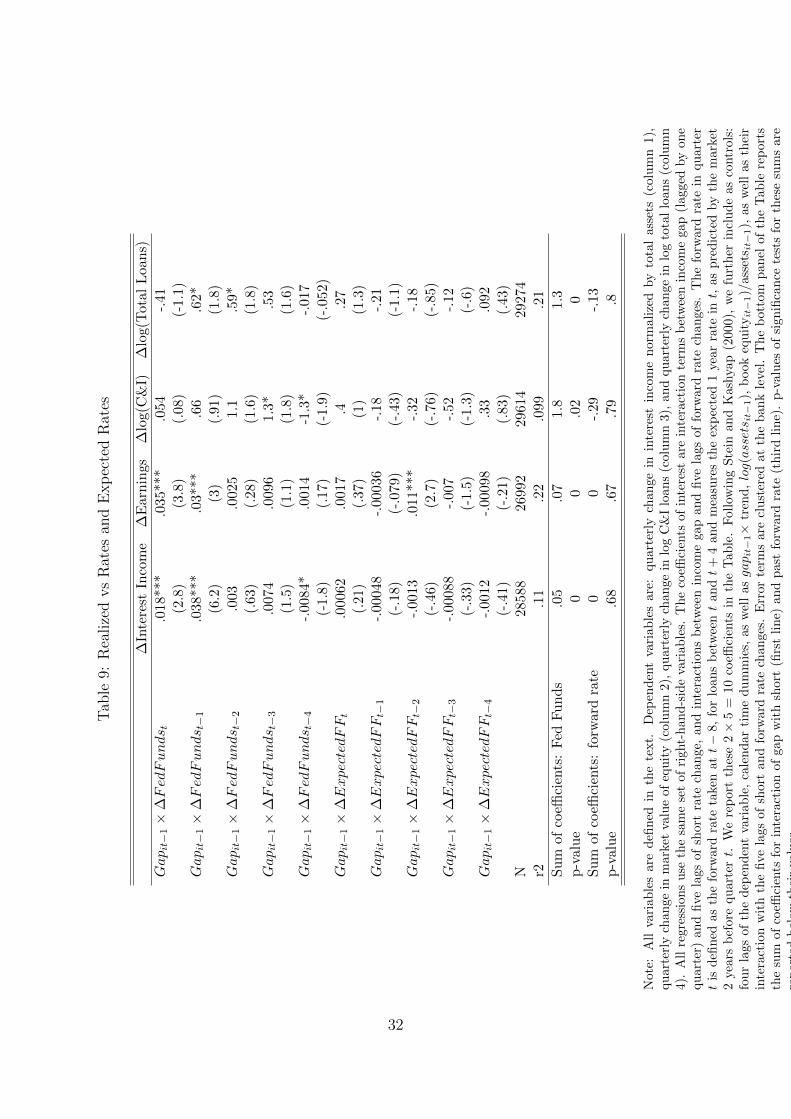
Tab

le9:

Realizedvs

Rates

andExp

ectedRates

∆Interest

Income

∆Earnings

∆log(C&I)

∆log(Total

Loa

ns)

Gap

it−1×

∆FedFunds

t.018

***

.035

***

.054

-.41

(2.8)

(3.8)

(.08

)(-1.1)

Gap

it−1×

∆FedFunds

t−1

.038

***

.03*

**.66

.62*

(6.2)

(3)

(.91

)(1.8)

Gap

it−1×

∆FedFunds

t−2

.003

.002

51.1

.59*

(.63

)(.28

)(1.6)

(1.8)

Gap

it−1×

∆FedFunds

t−3

.007

4.009

61.3*

.53

(1.5)

(1.1)

(1.8)

(1.6)

Gap

it−1×

∆FedFunds

t−4

-.00

84*

.001

4-1.3*

-.01

7(-1.8)

(.17

)(-1.9)

(-.052

)Gap

it−1×

∆ExpectedFFt

.000

62.001

7.4

.27

(.21

)(.37

)(1)

(1.3)

Gap

it−1×

∆ExpectedFFt−

1-.00

048

-.00

036

-.18

-.21

(-.18)

(-.079

)(-.43)

(-1.1)

Gap

it−1×

∆ExpectedFFt−

2-.00

13.011

***

-.32

-.18

(-.46)

(2.7)

(-.76)

(-.85)

Gap

it−1×

∆ExpectedFFt−

3-.00

088

-.00

7-.52

-.12

(-.33)

(-1.5)

(-1.3)

(-.6)

Gap

it−1×

∆ExpectedFFt−

4-.00

12-.00

098

.33

.092

(-.41)

(-.21)

(.83

)(.43

)N

2858

826

992

2961

429

274

r2.11

.22

.099

.21

Sum

ofcoeffi

cients:Fed

Funds

.05

.07

1.8

1.3

p-value

00

.02

0Sum

ofcoeffi

cients:forw

ardrate

00

-.29

-.13

p-value

.68

.67

.79

.8

Note:

Allvariab

lesaredefined

inthetext.Dep

endentvariab

lesare:

quarterlychan

gein

interest

incomenormalized

bytotalassets

(column1),

quarterlychan

gein

marketvalueof

equity(column2),qu

arterlychan

gein

logC&Iloan

s(column3),an

dqu

arterlychan

gein

logtotalloan

s(column

4).Allregression

suse

thesamesetof

righ

t-han

d-sidevariab

les.

Thecoeffi

cients

ofinterest

areinteractionterm

sbetweenincomegap(laggedby

one

quarter)

andfive

lags

ofshortrate

chan

ge,an

dinteractionsbetweenincomegapan

dfive

lags

offorw

ardrate

chan

ges.

Theforw

ardrate

inqu

arter

tis

defined

astheforw

ardrate

takenat

t−

8,forloan

sbetweentan

dt+

4an

dmeasurestheexpected1year

rate

int,as

predictedby

themarket

2yearsbeforequ

artert.

Wereportthese2×

5=

10coeffi

cients

intheTab

le.FollowingStein

andKashy

ap(2000),wefurther

includeas

controls:

fourlags

ofthedep

endentvariab

le,calendar

timedummies,

aswellas

gap i

t−1×

tren

d,log(assets

it−1),

boo

kequity i

t−1)/assets

it−1),

aswellas

their

interactionwiththefive

lags

ofshortan

dforw

ardrate

chan

ges.

Error

term

sareclustered

attheban

klevel.

Thebottom

pan

elof

theTab

lereports

thesum

ofcoeffi

cients

forinteractionof

gapwithshort(firstline)

andpastforw

ardrate

(thirdline).p-values

ofsign

ificance

testsforthesesumsare

reportedbelow

theirvalues.

32

A. Variable Definitions

This Section describes the construction of all variables in detail. i is an index for the bank,

t for the quarter.

A.1. Bank-level Variables

This Section gathers the variables constructed using the Consolidated Financial Statements

of Bank Holding Comanies (form FR Y-9C). Note that flow variables (interest and non-

interest income, earnings) are defined each quarter “year to date”. Hence, each time we

refer to a flow variable, we mean the quarterly, not year-to-date, flow. To transform a year-

to-date variable into a quarterly one, we take the variable as it is for the first quarter of each

year. For each quarter q = 2, 3, 4, we take the difference in the year-to-date variable between

q and q − 1.

• ∆Interestit: Change in interest income = [ interest income (bhck4107) at t + interest

expense (bhck4073) at t − 1 - interest income (bhck4107) at t − 1 - interest expense

(bhck4073) at t ] / ( total assets (bhck2170) taken in t− 1 ]. Note that bhck4073 and

bhck4107 have to be converted from year-to-date to quarterly as explained above.

• ∆Non Interestit: Change in non interest income = [ non interest income (bhck4079)

at t - non interest income (bhck4079) at t−1 ] / ( total assets (bhck2170) taken in t−1

]. Note that bhck4079 has to be converted from year-to-date to quarterly as explained

above.

• ∆Earningsit: Change in earnings = [ earnings (bhck4340) at t - earnings (bhck4340)

at t − 1 ] / ( total assets (bhck2170) taken in t − 1 ]. Note that bhck4340 has to be

converted from year-to-date to quarterly as explained above.

• ∆Valueit: Change in interest income = [ Equity market value at t - Equity market

value at t − 1 ] / ( total assets (bhck2170) taken in t − 1 ]. Equity market value is

33

obtained for publicly listed banks after matching with stock prices from CRSP. It is

equal to the number of shares outstanding (shrout) × the end-of-quarter closing price

(absolute value of prc).

• ∆log(C&I loansit): commercial and industrial loan growth = log[ C&I loans to US

adressees (bhck1763) at t + C&I loans to foreign adressees (bhck1764) at t ] - log[ C&I

loans to US adressees (bhck1763) at t− 1 + C&I loans to foreign adressees (bhck1764)

at t− 1 ].

• ∆log(Total loansit): Total loan growth = log [Total loans (bhck2122) at t ] - log[

Total loans (bhck2122) at t− 1 ].

• ∆Earningsit: Change in earnings = [ earnings (bhck4340) at t - earnings (bhck4340)

at t − 1 ] / ( total assets (bhck2170) taken in t − 1 ]. Note that bhck4340 has to be

converted from year-to-date to quarterly as explained above.

• Gapit−1: Income gap = [ assets that reprice or mature within one year (bhck31970)

- interest bearing deposits that reprice or mature whithin one year (bhck3296) - long

term debt that reprices within one year (bhck3298) - long term debt that matures

within one year (bhck3409) - variable rate preferred stock (bhck3408) ] / total assets

(bhck2170)

• Equityit−1: Equity ratio = 1 - [ total liabilities (bhck2948) / total assets (bhck2170) ]

• Sizeit−1: log ( total assets (bhck2170) )

• Liquidityit−1: Liquidity ratio = [ Available for sale securities (bhck1773)+ Held to

Maturity Securities (bhck1754) ] / total assets (bhck2170)

A.2. Times series Variables

This Section gathers different measures of interest rates used in the paper.

34

• ∆Fed Fundst: First difference between “effective federal funds” rate at t and t − 1.

Fed funds rates are available monthly from the Federal Reserve’s website: each quarter,

we take the observation corresponding to the last month.

• ∆10yrst: First difference between yields of 10 year treasury securities at t and t− 1,

available from the Federal Reserve’s website.

• ∆Expected FFt: Change in past “expected” 1 year interest rate between t − 1 and

t. Expected 1 year rate at t is obtained from the forward rate taken at t − 8 (two

years ago), for a loan between t and t + 3 (for the coming year). This forward rate is

computed using the Fama-Bliss discount bond prices. At date t− 8, we take the ratio

of the price of the 2-year to the 3-year zero-coupon bond, minus 1.

35

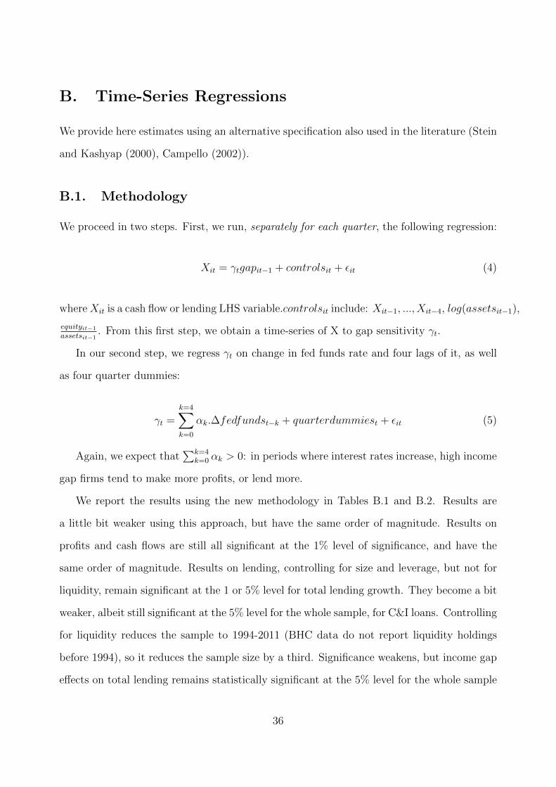
B. Time-Series Regressions

We provide here estimates using an alternative specification also used in the literature (Stein

and Kashyap (2000), Campello (2002)).

B.1. Methodology

We proceed in two steps. First, we run, separately for each quarter, the following regression:

Xit = γtgapit−1 + controlsit + �it (4)

whereXit is a cash flow or lending LHS variable.controlsit include: Xit−1, ..., Xit−4, log(assetsit−1),

equityit−1

assetsit−1. From this first step, we obtain a time-series of X to gap sensitivity γt.

In our second step, we regress γt on change in fed funds rate and four lags of it, as well

as four quarter dummies:

γt =k=4�

k=0

αk.∆fedfundst−k + quarterdummiest + �it (5)

Again, we expect that�k=4

k=0 αk > 0: in periods where interest rates increase, high income

gap firms tend to make more profits, or lend more.

We report the results using the new methodology in Tables B.1 and B.2. Results are

a little bit weaker using this approach, but have the same order of magnitude. Results on

profits and cash flows are still all significant at the 1% level of significance, and have the

same order of magnitude. Results on lending, controlling for size and leverage, but not for

liquidity, remain significant at the 1 or 5% level for total lending growth. They become a bit

weaker, albeit still significant at the 5% level for the whole sample, for C&I loans. Controlling

for liquidity reduces the sample to 1994-2011 (BHC data do not report liquidity holdings

before 1994), so it reduces the sample size by a third. Significance weakens, but income gap

effects on total lending remains statistically significant at the 5% level for the whole sample

36

and small firms, as well as firms with some interest rate derivative exposure. This alternative

estimation procedure provides estimates with very similar orders of magnitude.

B.2. Results

37

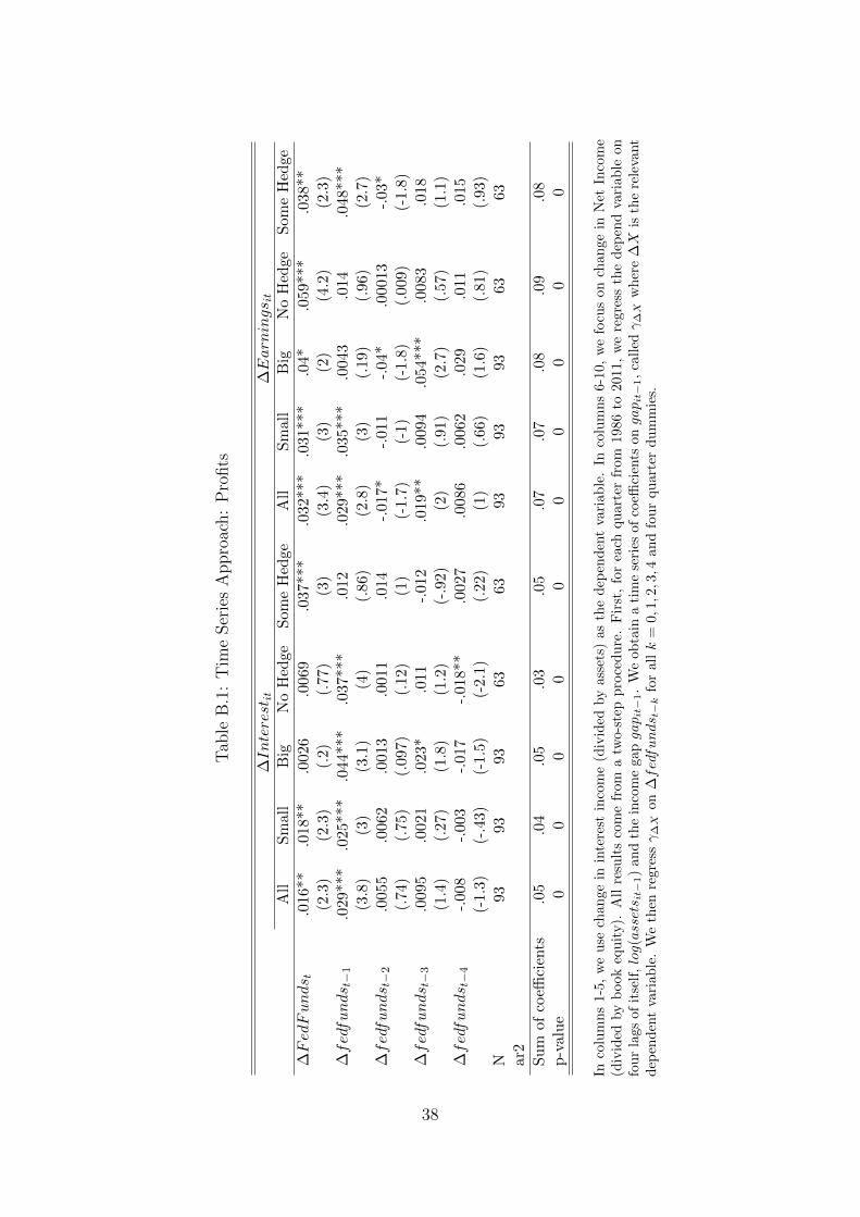
Tab

leB.1:Tim

eSeriesApproach:Profits

∆In

terest

it∆Ear

nings

it

All

Small

Big

NoHed

geSom

eHed

geAll

Small

Big

NoHed

geSom

eHed

ge∆FedFunds

t.016

**.018

**.002

6.006

9.037

***

.032

***

.031

***

.04*

.059

***

.038

**(2.3)

(2.3)

(.2)

(.77

)(3)

(3.4)

(3)

(2)

(4.2)

(2.3)

∆fedfunds

t−1

.029

***

.025

***

.044

***

.037

***

.012

.029

***

.035

***

.004

3.014

.048

***

(3.8)

(3)

(3.1)

(4)

(.86

)(2.8)

(3)

(.19

)(.96

)(2.7)

∆fedfunds

t−2

.005

5.006

2.001

3.001

1.014

-.01

7*-.01

1-.04

*.000

13-.03

*(.74

)(.75

)(.09

7)(.12

)(1)

(-1.7)

(-1)

(-1.8)

(.00

9)(-1.8)

∆fedfunds

t−3

.009

5.002

1.023

*.011

-.01

2.019

**.009

4.054

***

.008

3.018

(1.4)

(.27

)(1.8)

(1.2)

(-.92)

(2)

(.91

)(2.7)

(.57

)(1.1)

∆fedfunds

t−4

-.00

8-.00

3-.01

7-.01

8**

.002

7.008

6.006

2.029

.011

.015

(-1.3)

(-.43)

(-1.5)

(-2.1)

(.22

)(1)

(.66

)(1.6)

(.81

)(.93

)N

9393

9363

6393

9393

6363

ar2

Sum

ofcoeffi

cients

.05

.04

.05

.03

.05

.07

.07

.08

.09

.08

p-value

00

00

00

00

00

Incolumns1-5,

weuse

chan

gein

interest

income(divided

byassets)as

thedep

endentvariab

le.In

columns6-10,wefocuson

chan

gein

Net

Income

(divided

byboo

kequity).Allresultscomefrom

atw

o-step

procedure.First,foreach

quarterfrom

1986

to2011,weregressthedep

endvariab

leon

fourlags

ofitself,log(assets

it−1)an

dtheincomegapga

p it−

1.Weob

tain

atimeseries

ofcoeffi

cients

onga

p it−

1,called

γ ∆X

where∆X

istherelevant

dep

endentvariab

le.Wethen

regressγ ∆

Xon

∆fedfunds

t−kforallk=

0,1,2,3,4an

dfourqu

arterdummies.

38

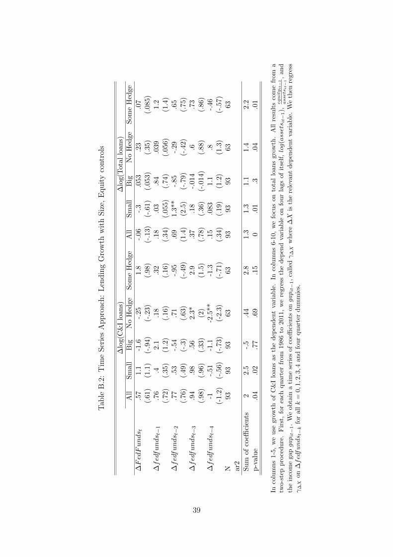
Tab

leB.2:Tim

eSeriesApproach:LendingGrowth

withSize,

Equ

itycontrols

∆log(C&Iloan

s)∆log(Total

loan

s)All

Small

Big

NoHed

geSom

eHed

geAll

Small

Big

NoHed

geSom

eHed

ge∆FedFunds

t.57

1.1

-1.6

-.25

1.8

-.06

-.3

.053

.23

.07

(.61

)(1.1)

(-.94)

(-.23)

(.98

)(-.13)

(-.61)

(.05

3)(.35

)(.08

5)∆fedfunds

t−1

.76

.42.1

.18

.32

.18

.03

.84

.039

1.2

(.72

)(.35

)(1.2)

(.16

)(.16

)(.34

)(.05

5)(.74

)(.05

6)(1.4)

∆fedfunds

t−2

.77

.53

-.54

.71

-.95

.69

1.3*

*-.85

-.29

.65

(.76

)(.49

)(-.3)

(.63

)(-.49)

(1.4)

(2.5)

(-.79)

(-.42)

(.75

)∆fedfunds

t−3

.94

.98

.56

2.3*

2.9

.37

.18

-.01

4.6

.73

(.98

)(.96

)(.33

)(2)

(1.5)

(.78

)(.36

)(-.014

)(.88

)(.86

)∆fedfunds

t−4

-1-.51

-1.1

-2.5**

-1.3

.15

.083

1.1

.8-.46

(-1.2)

(-.56)

(-.73)

(-2.3)

(-.71)

(.34

)(.19

)(1.2)

(1.3)

(-.57)

N93

9393

6363

9393

9363

63ar2

Sum

ofcoeffi

cients

22.5

-.5

.44

2.8

1.3

1.3

1.1

1.4

2.2

p-value

.04

.02

.77

.69

.15

0.01

.3.04

.01

Incolumns1-5,

weuse

grow

thof

C&Iloan

sas

thedep

endentvariab

le.In

columns6-10,wefocuson

totalloan

sgrow

th.Allresultscomefrom

atw

o-step

procedure.First,foreach

quarterfrom

1986

to2011,weregressthedep

endvariab

leon

fourlags

ofitself,log(assets

it−1),

equityit−

1

assets

it−

1,an

dtheincomegapga

p it−

1.Weob

tain

atimeseries

ofcoeffi

cients

onga

p it−

1,called

γ ∆X

where∆X

istherelevant

dep

endentvariab

le.Wethen

regress

γ ∆X

on∆fedfunds

t−kforallk=

0,1,2,3,4an

dfourqu

arterdummies.

39