basic statistical and modeling procedures using saskwelch/b600/2015/b600...1 basic statistical and...

1

Basic Statistical and Modeling Procedures Using SAS

One-Sample Tests

The statistical procedures illustrated in this handout use two datasets. The first, Pulse, has

information collected in a classroom setting, where students were asked to take their pulse two

times. Half the class was asked to run in place between the two readings and the other group was

asked to stay seated between the two readings. The raw data for this study are contained in a file

called pulse.csv. The other dataset we use is a dataset called Employee.sas7bdat. It is a SAS

dataset that contains information about salaries in a mythical company.

Read in the pulse data and create a temporary SAS dataset for the examples:

data pulse;

infile "pulse.csv" firstobs=2 delimiter="," missover;

input pulse1 pulse2 ran smokes sex height weight activity;

label pulse1 = "Resting pulse, rate per minute"

pulse2 = "Second pulse, rate per minute";

run;

Create and assign formats to variables:

proc format;

value sexfmt 1="Male" 2="Female";

value yesnofmt 1="Yes" 2="No";

value actfmt 1="Low" 2="Medium" 3="High";

run;

proc print data=pulse (obs=25) label;

format sex sexfmt. ran smokes yesnofmt. activity actfmt.;

run;

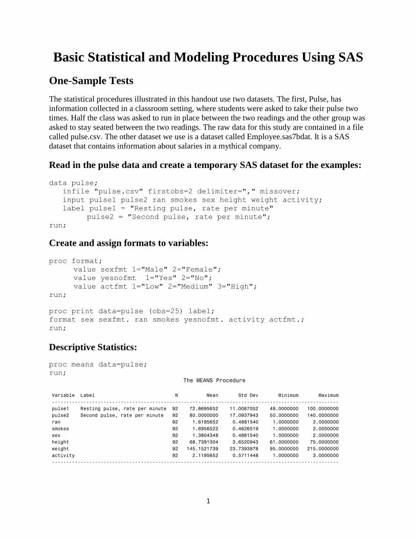
Descriptive Statistics:

proc means data=pulse;

run; The MEANS Procedure

Variable Label N Mean Std Dev Minimum Maximum

----------------------------------------------------------------------------------------------------

pulse1 Resting pulse, rate per minute 92 72.8695652 11.0087052 48.0000000 100.0000000

pulse2 Second pulse, rate per minute 92 80.0000000 17.0937943 50.0000000 140.0000000

ran 92 1.6195652 0.4881540 1.0000000 2.0000000

smokes 92 1.6956522 0.4626519 1.0000000 2.0000000

sex 92 1.3804348 0.4881540 1.0000000 2.0000000

height 92 68.7391304 3.6520943 61.0000000 75.0000000

weight 92 145.1521739 23.7393978 95.0000000 215.0000000

activity 92 2.1195652 0.5711448 1.0000000 3.0000000

----------------------------------------------------------------------------------------------------

2

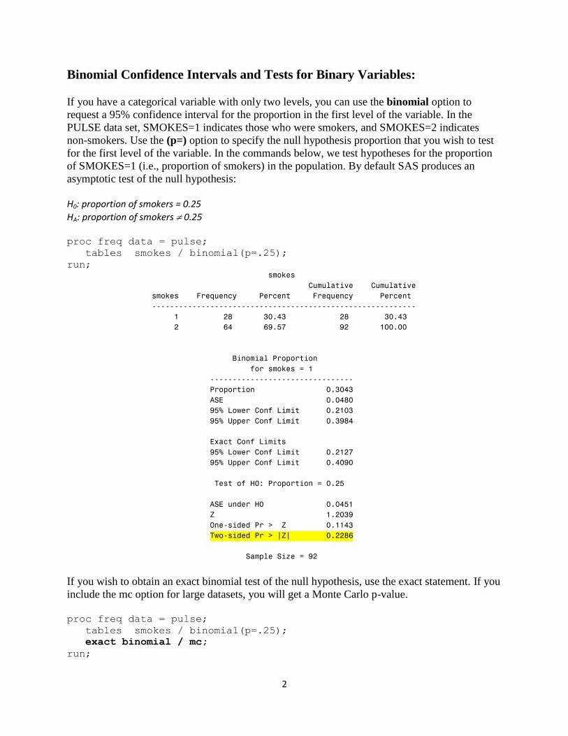
Binomial Confidence Intervals and Tests for Binary Variables: If you have a categorical variable with only two levels, you can use the binomial option to

request a 95% confidence interval for the proportion in the first level of the variable. In the

PULSE data set, SMOKES=1 indicates those who were smokers, and SMOKES=2 indicates

non-smokers. Use the (p=) option to specify the null hypothesis proportion that you wish to test

for the first level of the variable. In the commands below, we test hypotheses for the proportion

of SMOKES=1 (i.e., proportion of smokers) in the population. By default SAS produces an

asymptotic test of the null hypothesis: H0: proportion of smokers = 0.25

HA: proportion of smokers 0.25 proc freq data = pulse;

tables smokes / binomial(p=.25);

run; smokes

Cumulative Cumulative

smokes Frequency Percent Frequency Percent

-----------------------------------------------------------

1 28 30.43 28 30.43

2 64 69.57 92 100.00

Binomial Proportion

for smokes = 1

--------------------------------

Proportion 0.3043

ASE 0.0480

95% Lower Conf Limit 0.2103

95% Upper Conf Limit 0.3984

Exact Conf Limits



Test of H0: Proportion = 0.25

ASE under H0 0.0451

Z 1.2039

One-sided Pr > Z 0.1143

Two-sided Pr > |Z| 0.2286

Sample Size = 92

If you wish to obtain an exact binomial test of the null hypothesis, use the exact statement. If you

include the mc option for large datasets, you will get a Monte Carlo p-value. proc freq data = pulse;

tables smokes / binomial(p=.25);

exact binomial / mc;

run;

3

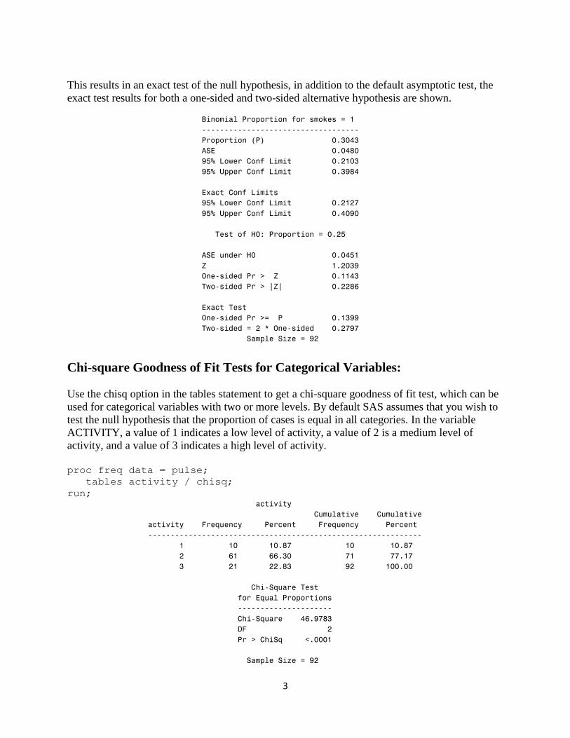
This results in an exact test of the null hypothesis, in addition to the default asymptotic test, the

exact test results for both a one-sided and two-sided alternative hypothesis are shown.

Binomial Proportion for smokes = 1

-----------------------------------

Proportion (P) 0.3043

ASE 0.0480



Exact Conf Limits



Test of H0: Proportion = 0.25

ASE under H0 0.0451

Z 1.2039

One-sided Pr > Z 0.1143

Two-sided Pr > |Z| 0.2286

Exact Test

One-sided Pr >= P 0.1399

Two-sided = 2 * One-sided 0.2797

Sample Size = 92

Chi-square Goodness of Fit Tests for Categorical Variables:

Use the chisq option in the tables statement to get a chi-square goodness of fit test, which can be

used for categorical variables with two or more levels. By default SAS assumes that you wish to

test the null hypothesis that the proportion of cases is equal in all categories. In the variable

ACTIVITY, a value of 1 indicates a low level of activity, a value of 2 is a medium level of

activity, and a value of 3 indicates a high level of activity. proc freq data = pulse;

tables activity / chisq;

run; activity


activity Frequency Percent Frequency Percent

-------------------------------------------------------------

1 10 10.87 10 10.87

2 61 66.30 71 77.17

3 21 22.83 92 100.00

Chi-Square Test

for Equal Proportions

---------------------

Chi-Square 46.9783

DF 2

Pr > ChiSq <.0001

Sample Size = 92

4

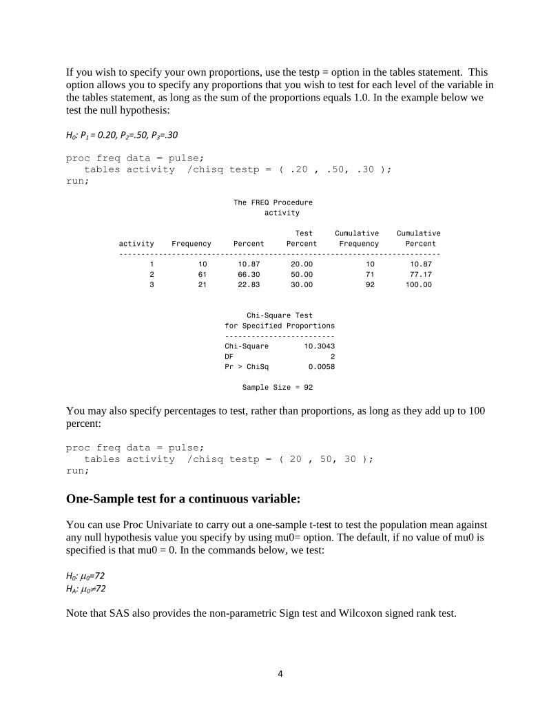
If you wish to specify your own proportions, use the testp = option in the tables statement. This

option allows you to specify any proportions that you wish to test for each level of the variable in

the tables statement, as long as the sum of the proportions equals 1.0. In the example below we

test the null hypothesis: H0: P1 = 0.20, P2=.50, P3=.30

proc freq data = pulse;

tables activity /chisq testp = ( .20 , .50, .30 );

run;

The FREQ Procedure

activity

Test Cumulative Cumulative

activity Frequency Percent Percent Frequency Percent

-------------------------------------------------------------------------

1 10 10.87 20.00 10 10.87

2 61 66.30 50.00 71 77.17

3 21 22.83 30.00 92 100.00

Chi-Square Test

for Specified Proportions

-------------------------

Chi-Square 10.3043

DF 2

Pr > ChiSq 0.0058

Sample Size = 92

You may also specify percentages to test, rather than proportions, as long as they add up to 100

percent: proc freq data = pulse;

tables activity /chisq testp = ( 20 , 50, 30 );

run;

One-Sample test for a continuous variable:

You can use Proc Univariate to carry out a one-sample t-test to test the population mean against

any null hypothesis value you specify by using mu0= option. The default, if no value of mu0 is

specified is that mu0 = 0. In the commands below, we test:

H0: 0=72

HA: 072

Note that SAS also provides the non-parametric Sign test and Wilcoxon signed rank test.

5

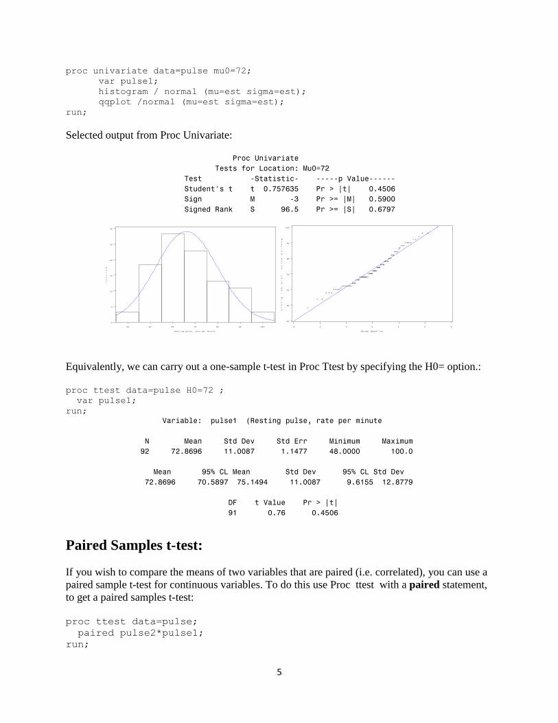
proc univariate data=pulse mu0=72;

var pulse1;

histogram / normal (mu=est sigma=est);

qqplot /normal (mu=est sigma=est);

run;

Selected output from Proc Univariate: Proc Univariate

Tests for Location: Mu0=72

Test -Statistic- -----p Value------

Student's t t 0.757635 Pr > |t| 0.4506

Sign M -3 Pr >= |M| 0.5900

Signed Rank S 96.5 Pr >= |S| 0.6797

5 2 6 0 6 8 7 6 8 4 9 2 1 0 0

0

5

1 0

1 5

2 0

2 5

3 0

P

e

r

c

e

n

t

Re s t i n g p u l s e , r a t e p e r mi n u t e - 3 - 2 - 1 0 1 2 3

4 0

5 0

6 0

7 0

8 0

9 0

1 0 0

R

e

s

t

i

n

g

p

u

l

s

e

,

r

a

t

e

p

e

r

m

i

n

u

t

e

No r ma l Qu a n t i l e s

Equivalently, we can carry out a one-sample t-test in Proc Ttest by specifying the H0= option.: proc ttest data=pulse H0=72 ;

var pulse1;

run;

Variable: pulse1 (Resting pulse, rate per minute

N Mean Std Dev Std Err Minimum Maximum

92 72.8696 11.0087 1.1477 48.0000 100.0

Mean 95% CL Mean Std Dev 95% CL Std Dev

72.8696 70.5897 75.1494 11.0087 9.6155 12.8779

DF t Value Pr > |t|

91 0.76 0.4506 Paired Samples t-test:

If you wish to compare the means of two variables that are paired (i.e. correlated), you can use a

paired sample t-test for continuous variables. To do this use Proc ttest with a paired statement,

to get a paired samples t-test: proc ttest data=pulse;

paired pulse2*pulse1;

run;

6

The TTEST Procedure

Statistics

Lower CL Upper CL Lower CL Upper CL

Difference N Mean Mean Mean Std Dev Std Dev Std Dev Std Err

pulse2 - pulse1 92 4.3406 7.1304 9.9203 11.766 13.471 15.759 1.4045

T-Tests

Difference DF t Value Pr > |t|

pulse2 - pulse1 91 5.08 <.0001

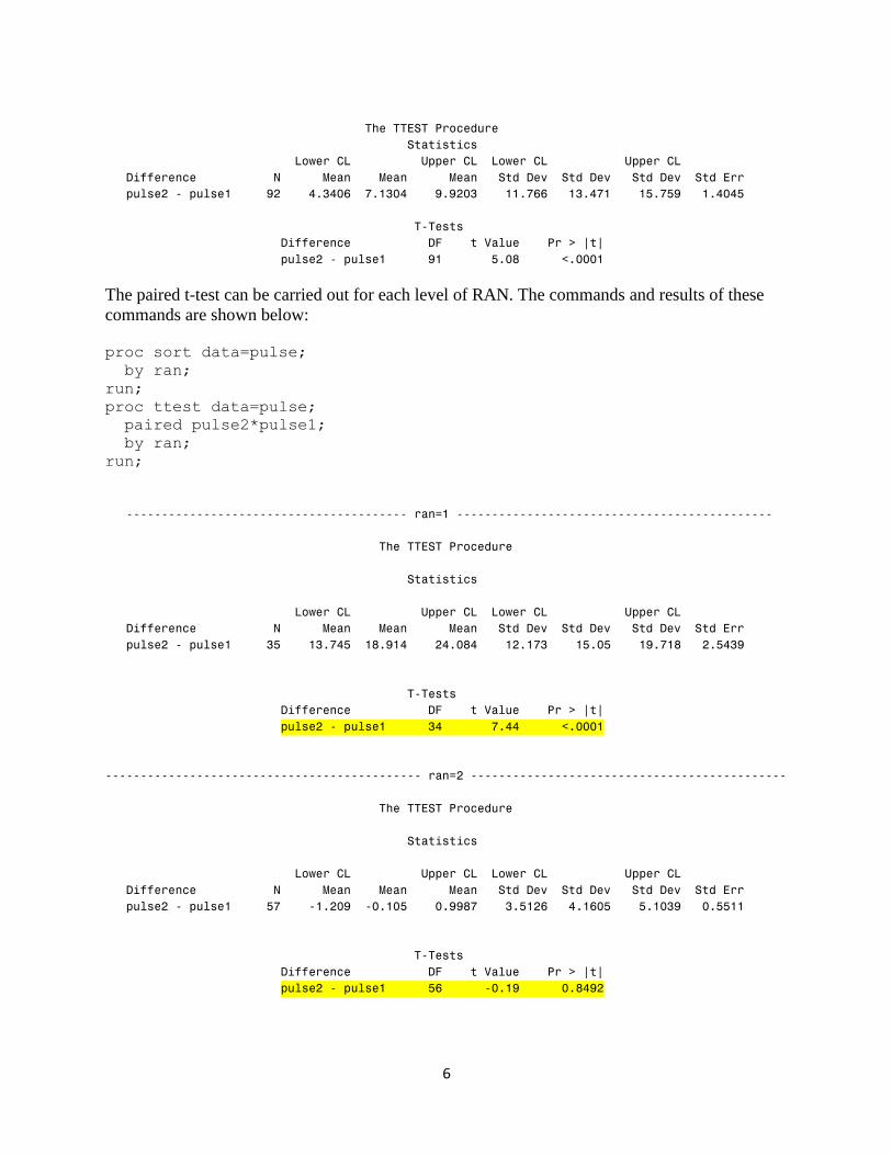
The paired t-test can be carried out for each level of RAN. The commands and results of these

commands are shown below:

proc sort data=pulse;

by ran;

run;

proc ttest data=pulse;

paired pulse2*pulse1;

by ran;

run;

---------------------------------------- ran=1 ---------------------------------------------

The TTEST Procedure

Statistics



pulse2 - pulse1 35 13.745 18.914 24.084 12.173 15.05 19.718 2.5439

T-Tests


pulse2 - pulse1 34 7.44 <.0001

--------------------------------------------- ran=2 ---------------------------------------------

The TTEST Procedure

Statistics



pulse2 - pulse1 57 -1.209 -0.105 0.9987 3.5126 4.1605 5.1039 0.5511

T-Tests


pulse2 - pulse1 56 -0.19 0.8492

7

Independent samples t-tests

An independent samples t-test can be used to compare the means in two independent groups of

observations.:

proc ttest data=sasdata2.employee2;

class gender;

var salary;

run;

The output from this procedure is shown below: The TTEST Procedure

Variable: salary (Current Salary)

gender N Mean Std Dev Std Err Minimum Maximum

f 216 26031.9 7558.0 514.3 15750.0 58125.0

m 258 41441.8 19499.2 1214.0 19650.0 135000

Diff (1-2) -15409.9 15265.9 1407.9

gender Method Mean 95% CL Mean Std Dev 95% CL Std Dev

f 26031.9 25018.3 27045.6 7558.0 6906.2 8346.8

m 41441.8 39051.2 43832.4 19499.2 17949.3 21344.3

Diff (1-2) Pooled -15409.9 -18176.4 -12643.3 15265.9 14351.1 16306.1

Diff (1-2) Satterthwaite -15409.9 -18003.0 -12816.7

Method Variances DF t Value Pr > |t|

Pooled Equal 472 -10.95 <.0001

Satterthwaite Unequal 344.26 -11.69 <.0001

Equality of Variances

Method Num DF Den DF F Value Pr > F

Folded F 257 215 6.66 <.0001

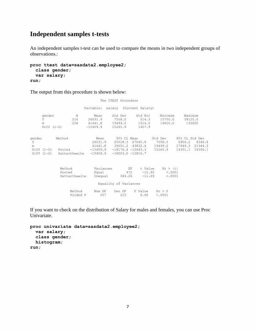
If you want to check on the distribution of Salary for males and females, you can use Proc

Univariate.

proc univariate data=sasdata2.employee2;

var salary;

class gender;

histogram;

run;

8

0

10

20

30

40

50

Perc

ent

Fe

ma

le

$17,500 $32,500 $47,500 $62,500 $77,500 $92,500 $107,500 $122,500

0

10

20

30

40

50

Perc

ent

Ma

le

Current Salary

Ge

nd

er

Because it looks like salary is highly skewed, you might want to use a log transformation of

salary to compare the two genders. Proc ttest has the dist=lognormal option to accompllish

this:

proc ttest data=sasdata2.employee2 dist=lognormal;

class gender;

var salary ;

run;

The output from this procedure shows that the geometric mean and coefficient of variation are

reported, rather than the arithmetic mean and standard deviation.

Variable: salary (Current Salary)

Geometric Coefficient

gender N Mean of Variation Minimum Maximum

Female 216 25146.1 0.2582 15750.0 58125.0

Male 258 37972.2 0.4149 19650.0 135000

Ratio (1/2) 0.6622 0.3505

Geometric Coefficient

gender Method Mean 95% CL Mean of Variation 95% CL CV

Female 25146.1 24303.8 26017.5 0.2582 0.2353 0.2862

Male 37972.2 36161.3 39873.8 0.4149 0.3796 0.4579

Ratio (1/2) Pooled 0.6622 0.6226 0.7044 0.3505 0.3284 0.3760

Ratio (1/2) Satterthwaite 0.6622 0.6240 0.7028

Coefficients

Method of Variation DF t Value Pr > |t|

Pooled Equal 472 -13.13 <.0001

Satterthwaite Unequal 442.4 -13.63 <.0001

9

Equality of Variances

Method Num DF Den DF F Value Pr > F

Folded F 257 215 2.46 <.0001

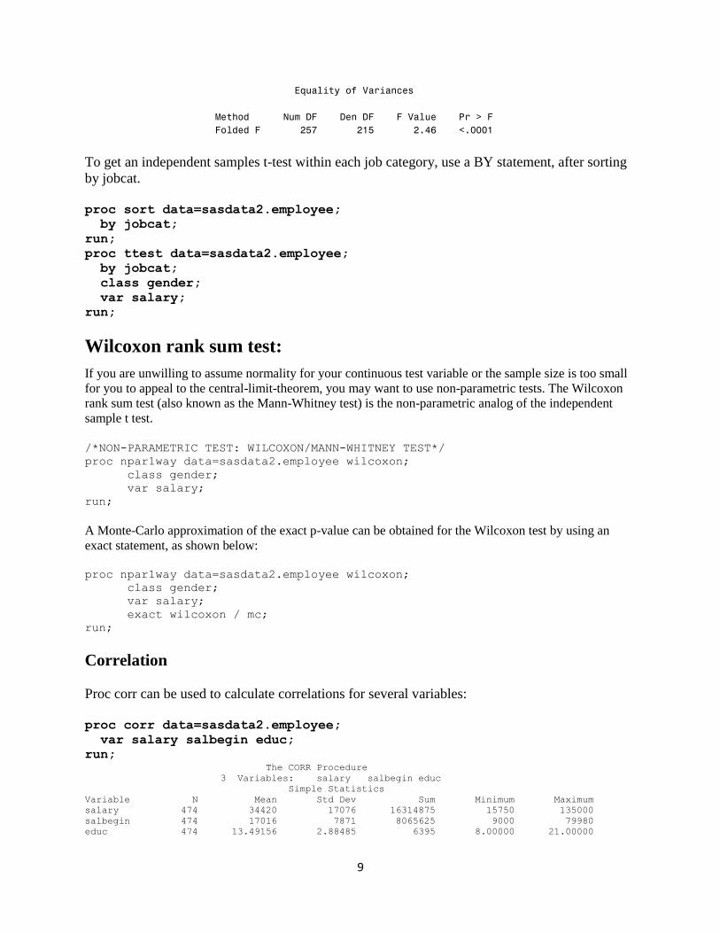
To get an independent samples t-test within each job category, use a BY statement, after sorting

by jobcat.

proc sort data=sasdata2.employee;

by jobcat;

run;

proc ttest data=sasdata2.employee;

by jobcat;

class gender;

var salary;

run;

Wilcoxon rank sum test:

If you are unwilling to assume normality for your continuous test variable or the sample size is too small

for you to appeal to the central-limit-theorem, you may want to use non-parametric tests. The Wilcoxon

rank sum test (also known as the Mann-Whitney test) is the non-parametric analog of the independent

sample t test.

/*NON-PARAMETRIC TEST: WILCOXON/MANN-WHITNEY TEST*/

proc npar1way data=sasdata2.employee wilcoxon;

class gender;

var salary;

run;

A Monte-Carlo approximation of the exact p-value can be obtained for the Wilcoxon test by using an

exact statement, as shown below:

proc npar1way data=sasdata2.employee wilcoxon;

class gender;

var salary;

exact wilcoxon / mc;

run;

Correlation

Proc corr can be used to calculate correlations for several variables:

proc corr data=sasdata2.employee;

var salary salbegin educ;

run; The CORR Procedure

3 Variables: salary salbegin educ

Simple Statistics

Variable N Mean Std Dev Sum Minimum Maximum

salary 474 34420 17076 16314875 15750 135000

salbegin 474 17016 7871 8065625 9000 79980

educ 474 13.49156 2.88485 6395 8.00000 21.00000

10

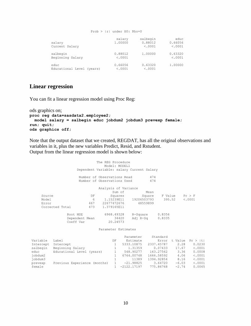
Prob > |r| under H0: Rho=0

salary salbegin educ

salary 1.00000 0.88012 0.66056

Current Salary <.0001 <.0001

salbegin 0.88012 1.00000 0.63320

Beginning Salary <.0001 <.0001

educ 0.66056 0.63320 1.00000

Educational Level (years) <.0001 <.0001

Linear regression

You can fit a linear regression model using Proc Reg:

ods graphics on; proc reg data=sasdata2.employee2;

model salary = salbegin educ jobdum2 jobdum3 prevexp female;

run; quit;

ods graphics off;

Note that the output dataset that we created, REGDAT, has all the original observations and

variables in it, plus the new variables Predict, Resid, and Rstudent.

Output from the linear regression model is shown below:

The REG Procedure

Model: MODEL1

Dependent Variable: salary Current Salary

Number of Observations Read 474

Number of Observations Used 474

Analysis of Variance

Sum of Mean

Source DF Squares Square F Value Pr > F

Model 6 1.15239E11 19206503793 395.52 <.0001

Error 467 22677472676 48559899

Corrected Total 473 1.379165E11

Root MSE 6968.49328 R-Square 0.8356

Dependent Mean 34420 Adj R-Sq 0.8335

Coeff Var 20.24573

Parameter Estimates

Parameter Standard

Variable Label DF Estimate Error t Value Pr > |t|

Intercept Intercept 1 5333.10875 2337.45787 2.28 0.0230

salbegin Beginning Salary 1 1.31359 0.07433 17.67 <.0001

educ Educational Level (years) 1 548.90277 163.27562 3.36 0.0008

jobdum2 1 6764.00748 1666.58592 4.06 <.0001

jobdum3 1 11389 1394.92854 8.16 <.0001

prevexp Previous Experience (months) 1 -21.98825 3.64720 -6.03 <.0001

female 1 -2122.17197 775.86768 -2.74 0.0065

11

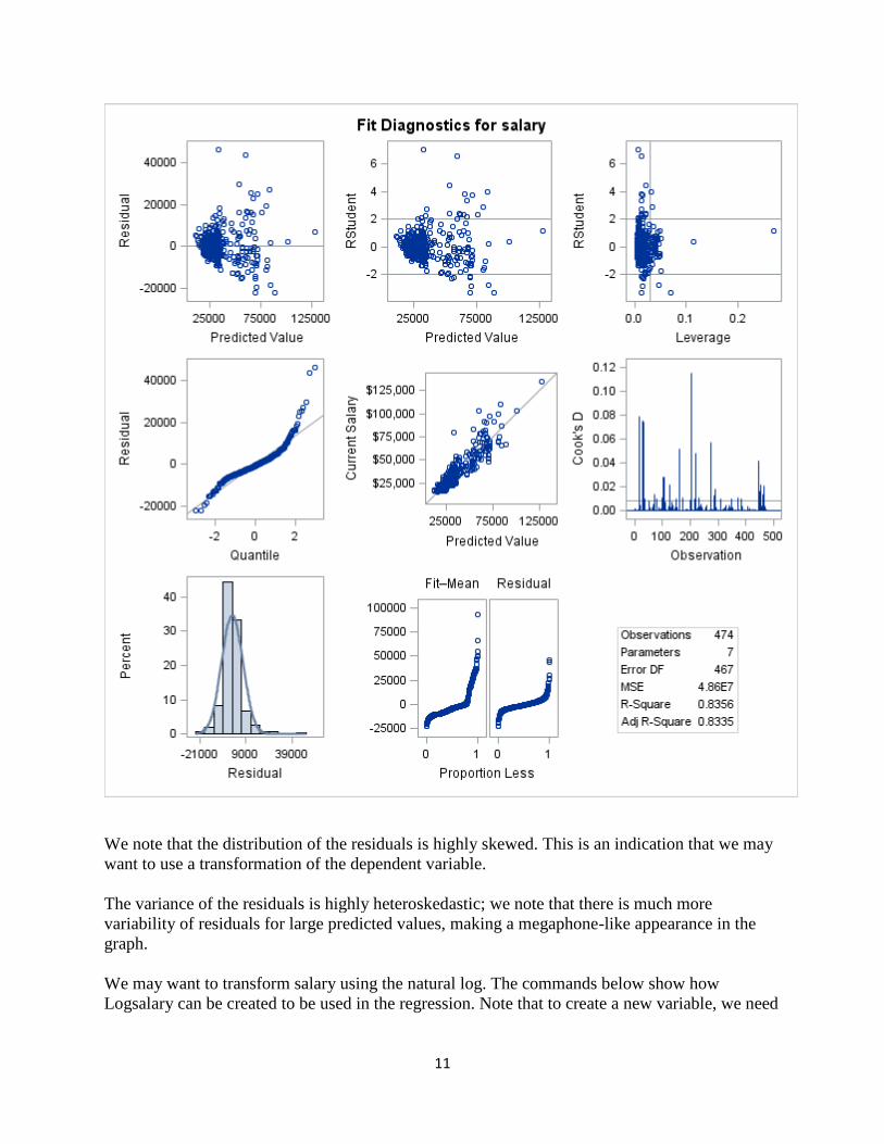
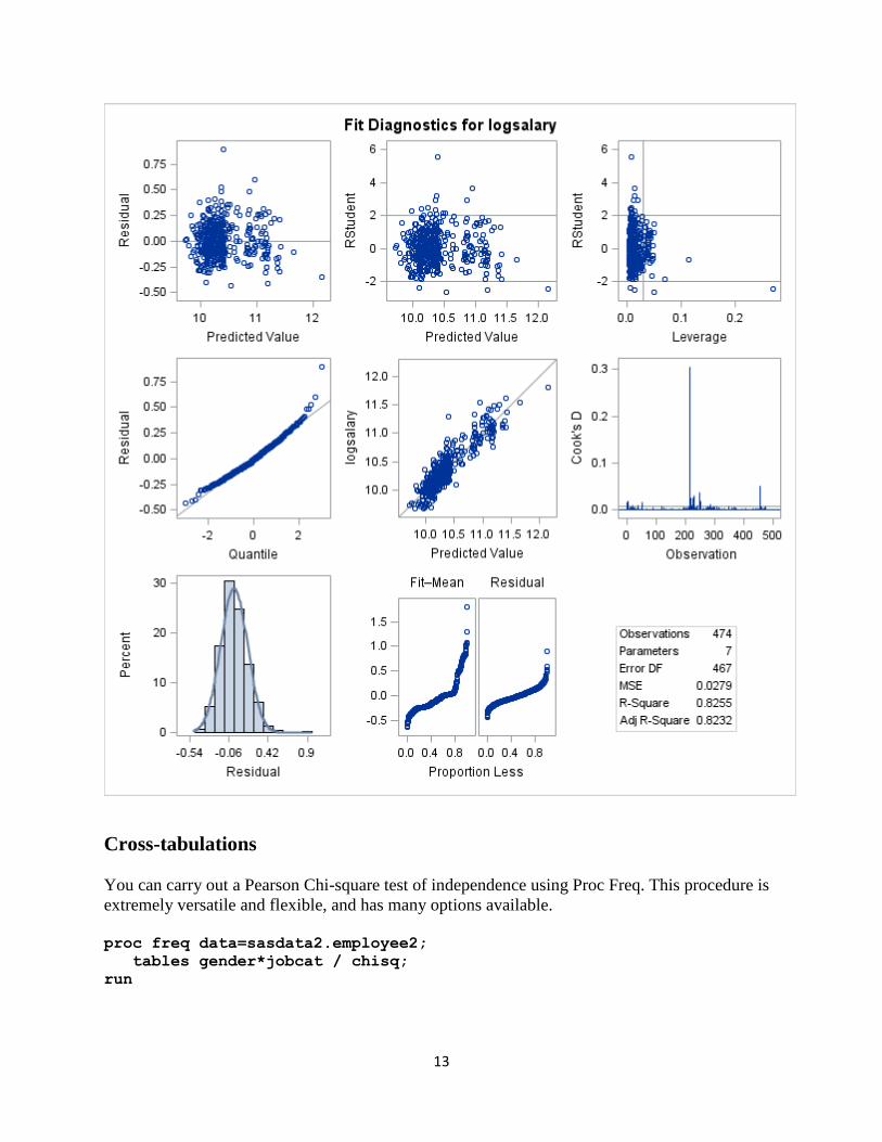
We note that the distribution of the residuals is highly skewed. This is an indication that we may

want to use a transformation of the dependent variable.

The variance of the residuals is highly heteroskedastic; we note that there is much more

variability of residuals for large predicted values, making a megaphone-like appearance in the

graph.

We may want to transform salary using the natural log. The commands below show how

Logsalary can be created to be used in the regression. Note that to create a new variable, we need

12

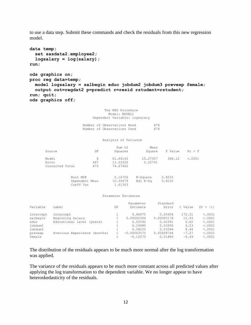
to use a data step. Submit these commands and check the residuals from this new regression

model.

data temp;

set sasdata2.employee2;

logsalary = log(salary);

run;

ods graphics on;

proc reg data=temp;

model logsalary = salbegin educ jobdum2 jobdum3 prevexp female;

output out=regdat2 p=predict r=resid rstudent=rstudent;

run; quit;

ods graphics off;

The REG Procedure

Model: MODEL1

Dependent Variable: logsalary



Analysis of Variance

Sum of Mean

Source DF Squares Square F Value Pr > F

Model 6 61.64142 10.27357 368.12 <.0001

Error 467 13.03320 0.02791

Corrected Total 473 74.67462

Root MSE 0.16706 R-Square 0.8255

Dependent Mean 10.35679 Adj R-Sq 0.8232

Coeff Var 1.61303

Parameter Estimates

Parameter Standard

Variable Label DF Estimate Error t Value Pr > |t|

Intercept Intercept 1 9.66675 0.05604 172.51 <.0001

salbegin Beginning Salary 1 0.00002304 0.00000178 12.93 <.0001

educ Educational Level (years) 1 0.02592 0.00391 6.62 <.0001

jobdum2 1 0.24880 0.03995 6.23 <.0001

jobdum3 1 0.28225 0.03344 8.44 <.0001

prevexp Previous Experience (months) 1 -0.00063575 0.00008744 -7.27 <.0001

female 1 -0.12070 0.01860 -6.49 <.0001

The distribution of the residuals appears to be much more normal after the log transformation

was applied.

The variance of the residuals appears to be much more constant across all predicted values after

applying the log transformation to the dependent variable. We no longer appear to have

heteroskedasticity of the residuals.

13

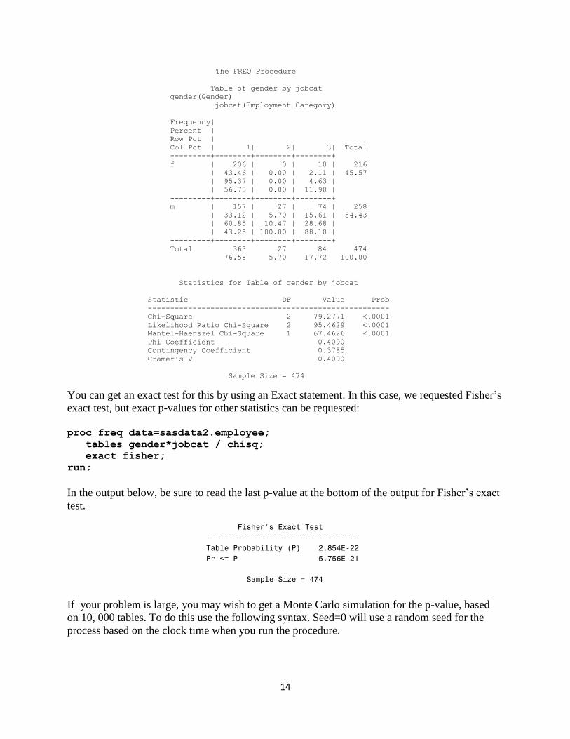
Cross-tabulations

You can carry out a Pearson Chi-square test of independence using Proc Freq. This procedure is

extremely versatile and flexible, and has many options available.

proc freq data=sasdata2.employee2;

tables gender*jobcat / chisq;

run

14

The FREQ Procedure

Table of gender by jobcat

gender(Gender)

jobcat(Employment Category)

Frequency|

Percent |

Row Pct |

Col Pct | 1| 2| 3| Total

---------+--------+--------+--------+

f | 206 | 0 | 10 | 216

| 43.46 | 0.00 | 2.11 | 45.57

| 95.37 | 0.00 | 4.63 |

| 56.75 | 0.00 | 11.90 |

---------+--------+--------+--------+

m | 157 | 27 | 74 | 258

| 33.12 | 5.70 | 15.61 | 54.43

| 60.85 | 10.47 | 28.68 |

| 43.25 | 100.00 | 88.10 |

---------+--------+--------+--------+

Total 363 27 84 474

76.58 5.70 17.72 100.00

Statistics for Table of gender by jobcat

Statistic DF Value Prob

------------------------------------------------------

Chi-Square 2 79.2771 <.0001

Likelihood Ratio Chi-Square 2 95.4629 <.0001

Mantel-Haenszel Chi-Square 1 67.4626 <.0001

Phi Coefficient 0.4090

Contingency Coefficient 0.3785

Cramer's V 0.4090

Sample Size = 474

You can get an exact test for this by using an Exact statement. In this case, we requested Fisher’s

exact test, but exact p-values for other statistics can be requested:

proc freq data=sasdata2.employee;


exact fisher;

run;

In the output below, be sure to read the last p-value at the bottom of the output for Fisher’s exact

test.

Fisher's Exact Test

----------------------------------

Table Probability (P) 2.854E-22

Pr <= P 5.756E-21

Sample Size = 474

If your problem is large, you may wish to get a Monte Carlo simulation for the p-value, based

on 10, 000 tables. To do this use the following syntax. Seed=0 will use a random seed for the

process based on the clock time when you run the procedure.

15



exact fisher / mc seed=0;

run;

Partial output from this procedure is shown below:

The FREQ Procedure

Statistics for Table of gender by jobcat

Fisher's Exact Test

----------------------------------

Table Probability (P) 2.854E-22

Monte Carlo Estimate for the Exact Test

Pr <= P 0.0000


99% Upper Conf Limit 4.604E-04

Number of Samples 10000

Initial Seed 445615001

Sample Size = 474

Each time the procedure is run using this syntax, you will get different answers. If you wish to

get the same result, simply use the Initial Seed value reported by SAS in the output in your Exact

statement.



exact fisher / mc seed=445615001;

run;

McNemar’s test for paired categorical data:

If you wish to compare the proportions in a 2 by 2 table for paired data, you can use McNemar’s

test, by specifying the agree option in Proc Freq. Before running the McNemar’s test, we recode

PULSE1 and PULSE2 into two categorical variables HIPULSE1 and HIPULSE2, as shown

below: data newpulse;

set pulse;

if pulse1 > 80 then hipulse1 = 1;

if pulse1 > 0 and pulse1 <=89 then hipulse1=0;

if pulse2 > 80 then hipulse2 = 1;

if pulse2 > 0 and pulse2 <=89 then hipulse2=0;

run;

16

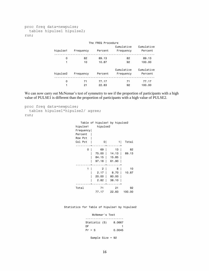
proc freq data=newpulse;

tables hipulse1 hipulse2;

run;

The FREQ Procedure


hipulse1 Frequency Percent Frequency Percent

-------------------------------------------------------------

0 82 89.13 82 89.13

1 10 10.87 92 100.00


hipulse2 Frequency Percent Frequency Percent

-------------------------------------------------------------

0 71 77.17 71 77.17

1 21 22.83 92 100.00

We can now carry out McNemar’s test of symmetry to see if the proportion of participants with a high

value of PULSE1 is different than the proportion of participants with a high value of PULSE2.

proc freq data=newpulse;

tables hipulse1*hipulse2/ agree;

run;

Table of hipulse1 by hipulse2

hipulse1 hipulse2

Frequency|

Percent |

Row Pct |

Col Pct | 0| 1| Total

---------+--------+--------+

0 | 69 | 13 | 82

| 75.00 | 14.13 | 89.13

| 84.15 | 15.85 |

| 97.18 | 61.90 |

---------+--------+--------+

1 | 2 | 8 | 10

| 2.17 | 8.70 | 10.87

| 20.00 | 80.00 |

| 2.82 | 38.10 |

---------+--------+--------+

Total 71 21 92

77.17 22.83 100.00

Statistics for Table of hipulse1 by hipulse2

McNemar's Test

-----------------------

Statistic (S) 8.0667

DF 1

Pr > S 0.0045

Sample Size = 92

17

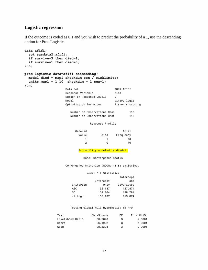
Logistic regression

If the outcome is coded as 0,1 and you wish to predict the probability of a 1, use the descending

option for Proc Logistic.

data afifi;

set sasdata2.afifi;

if survive=3 then died=1;

if survive=1 then died=0;

run;

proc logistic data=afifi descending;

model died = map1 shockdum sex / risklimits;

units map1 = 1 10 shockdum = 1 sex=1;

run; Data Set WORK.AFIFI

Response Variable died

Number of Response Levels 2

Model binary logit

Optimization Technique Fisher's scoring



Response Profile

Ordered Total

Value died Frequency

1 1 43

2 0 70

Probability modeled is died=1.

Model Convergence Status

Convergence criterion (GCONV=1E-8) satisfied.

Model Fit Statistics

Intercept

Intercept and

Criterion Only Covariates

AIC 152.137 127.874

SC 154.864 138.784

-2 Log L 150.137 119.874

Testing Global Null Hypothesis: BETA=0

Test Chi-Square DF Pr > ChiSq

Likelihood Ratio 30.2628 3 <.0001

Score 26.1922 3 <.0001

Wald 20.3328 3 0.0001

18

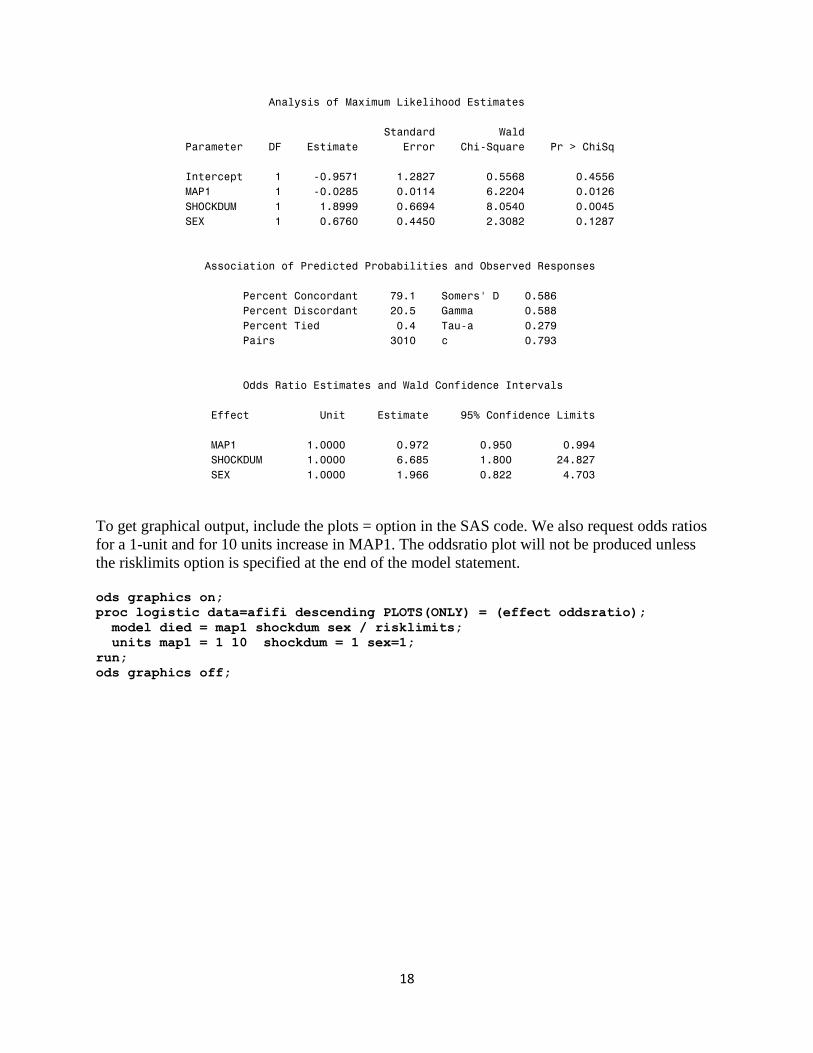
Analysis of Maximum Likelihood Estimates

Standard Wald

Parameter DF Estimate Error Chi-Square Pr > ChiSq

Intercept 1 -0.9571 1.2827 0.5568 0.4556

MAP1 1 -0.0285 0.0114 6.2204 0.0126

SHOCKDUM 1 1.8999 0.6694 8.0540 0.0045

SEX 1 0.6760 0.4450 2.3082 0.1287

Association of Predicted Probabilities and Observed Responses

Percent Concordant 79.1 Somers' D 0.586

Percent Discordant 20.5 Gamma 0.588

Percent Tied 0.4 Tau-a 0.279

Pairs 3010 c 0.793

Odds Ratio Estimates and Wald Confidence Intervals

Effect Unit Estimate 95% Confidence Limits

MAP1 1.0000 0.972 0.950 0.994

SHOCKDUM 1.0000 6.685 1.800 24.827

SEX 1.0000 1.966 0.822 4.703

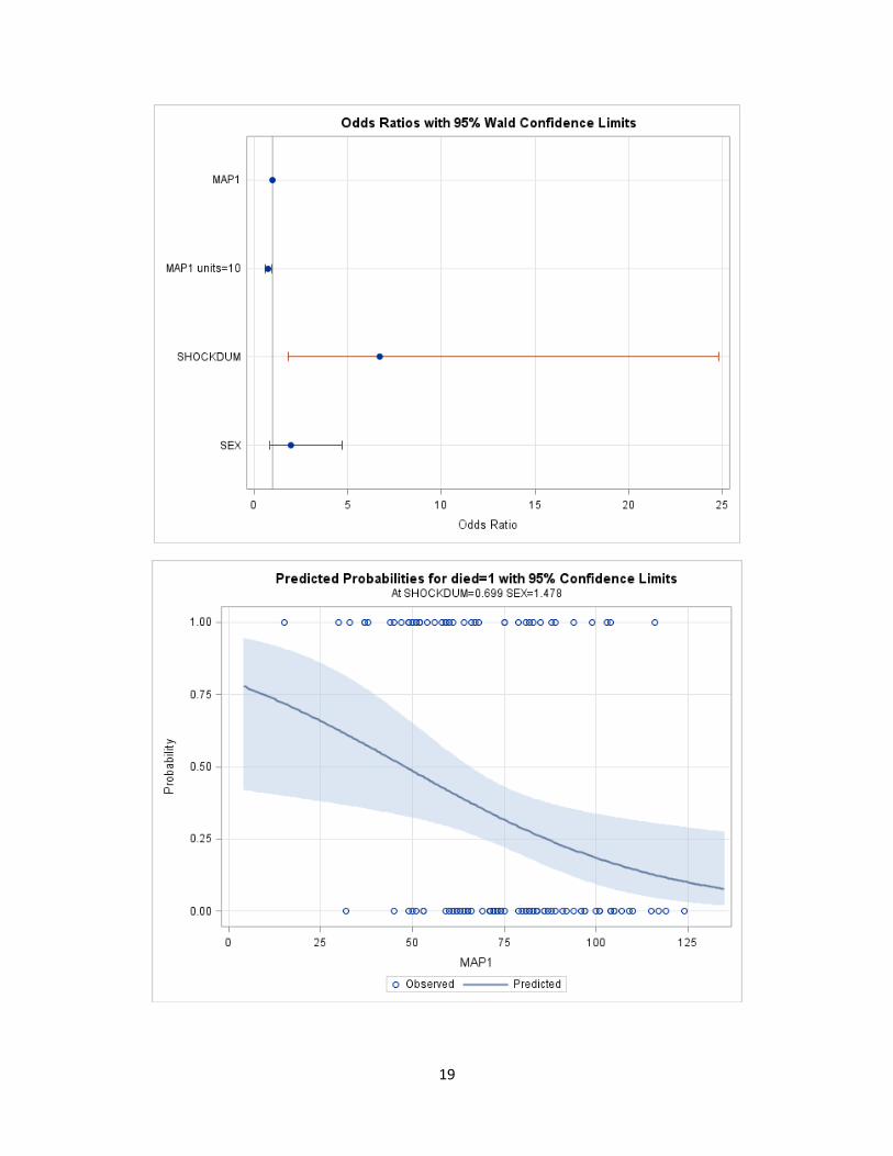
To get graphical output, include the plots = option in the SAS code. We also request odds ratios

for a 1-unit and for 10 units increase in MAP1. The oddsratio plot will not be produced unless

the risklimits option is specified at the end of the model statement.

ods graphics on;

proc logistic data=afifi descending PLOTS(ONLY) = (effect oddsratio);

model died = map1 shockdum sex / risklimits;

units map1 = 1 10 shockdum = 1 sex=1;

run;

ods graphics off;

20

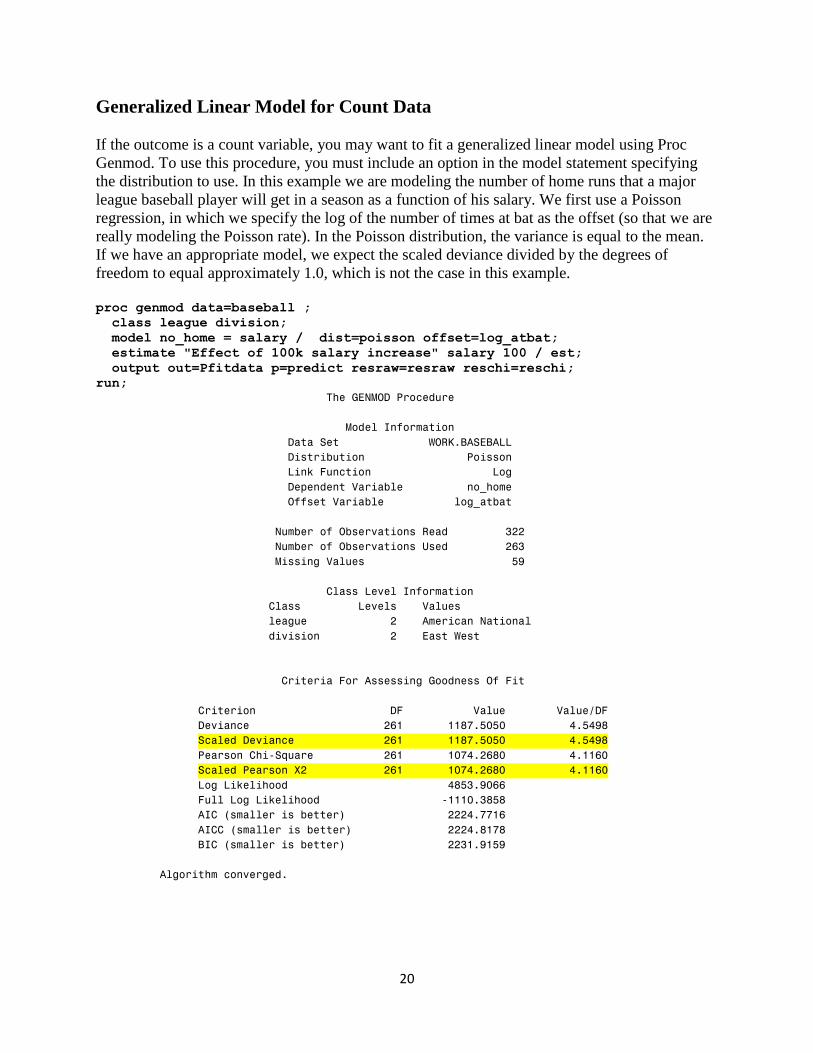
Generalized Linear Model for Count Data

If the outcome is a count variable, you may want to fit a generalized linear model using Proc

Genmod. To use this procedure, you must include an option in the model statement specifying

the distribution to use. In this example we are modeling the number of home runs that a major

league baseball player will get in a season as a function of his salary. We first use a Poisson

regression, in which we specify the log of the number of times at bat as the offset (so that we are

really modeling the Poisson rate). In the Poisson distribution, the variance is equal to the mean.

If we have an appropriate model, we expect the scaled deviance divided by the degrees of

freedom to equal approximately 1.0, which is not the case in this example.

proc genmod data=baseball ;

class league division;

model no_home = salary / dist=poisson offset=log_atbat;

estimate "Effect of 100k salary increase" salary 100 / est;

output out=Pfitdata p=predict resraw=resraw reschi=reschi;

run; The GENMOD Procedure

Model Information

Data Set WORK.BASEBALL

Distribution Poisson

Link Function Log

Dependent Variable no_home

Offset Variable log_atbat



Missing Values 59

Class Level Information

Class Levels Values

league 2 American National

division 2 East West

Criteria For Assessing Goodness Of Fit

Criterion DF Value Value/DF

Deviance 261 1187.5050 4.5498

Scaled Deviance 261 1187.5050 4.5498

Pearson Chi-Square 261 1074.2680 4.1160

Scaled Pearson X2 261 1074.2680 4.1160

Log Likelihood 4853.9066

Full Log Likelihood -1110.3858

AIC (smaller is better) 2224.7716

AICC (smaller is better) 2224.8178

BIC (smaller is better) 2231.9159

Algorithm converged.

21

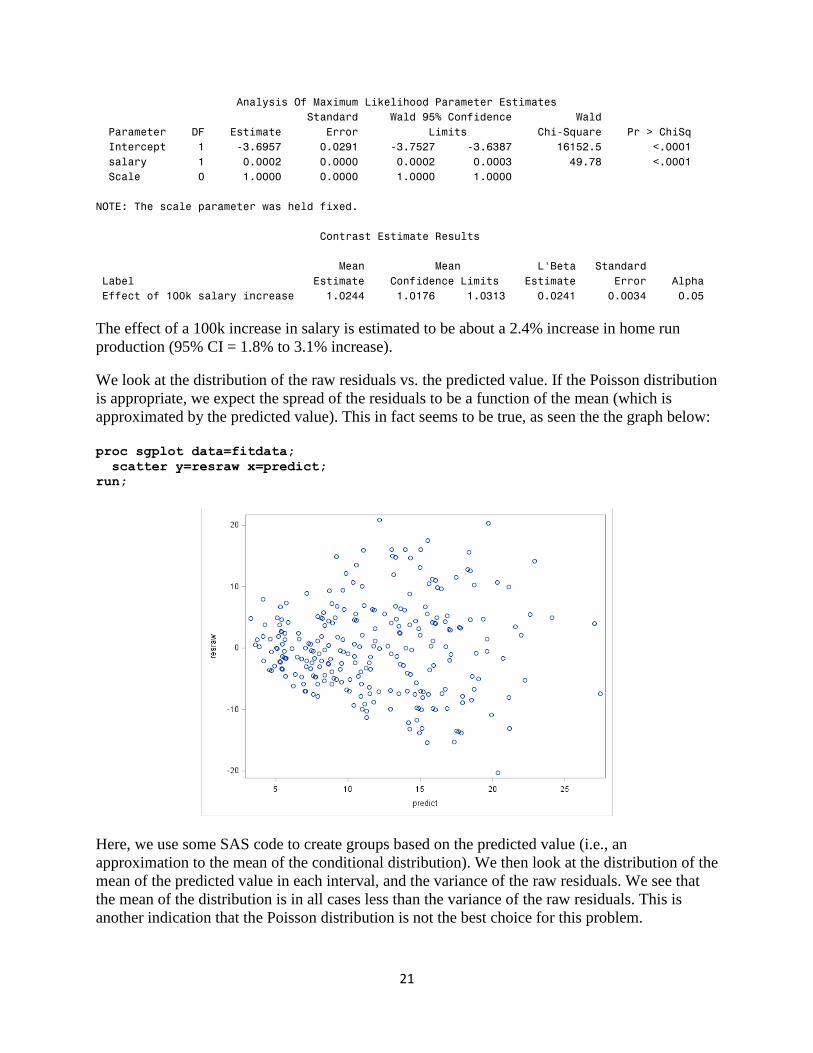
Analysis Of Maximum Likelihood Parameter Estimates

Standard Wald 95% Confidence Wald

Parameter DF Estimate Error Limits Chi-Square Pr > ChiSq

Intercept 1 -3.6957 0.0291 -3.7527 -3.6387 16152.5 <.0001

salary 1 0.0002 0.0000 0.0002 0.0003 49.78 <.0001

Scale 0 1.0000 0.0000 1.0000 1.0000

NOTE: The scale parameter was held fixed.

Contrast Estimate Results

Mean Mean L'Beta Standard

Label Estimate Confidence Limits Estimate Error Alpha

Effect of 100k salary increase 1.0244 1.0176 1.0313 0.0241 0.0034 0.05

The effect of a 100k increase in salary is estimated to be about a 2.4% increase in home run

production (95% CI = 1.8% to 3.1% increase).

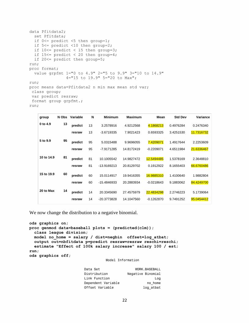
We look at the distribution of the raw residuals vs. the predicted value. If the Poisson distribution

is appropriate, we expect the spread of the residuals to be a function of the mean (which is

approximated by the predicted value). This in fact seems to be true, as seen the the graph below:

proc sgplot data=fitdata;

scatter y=resraw x=predict;

run;

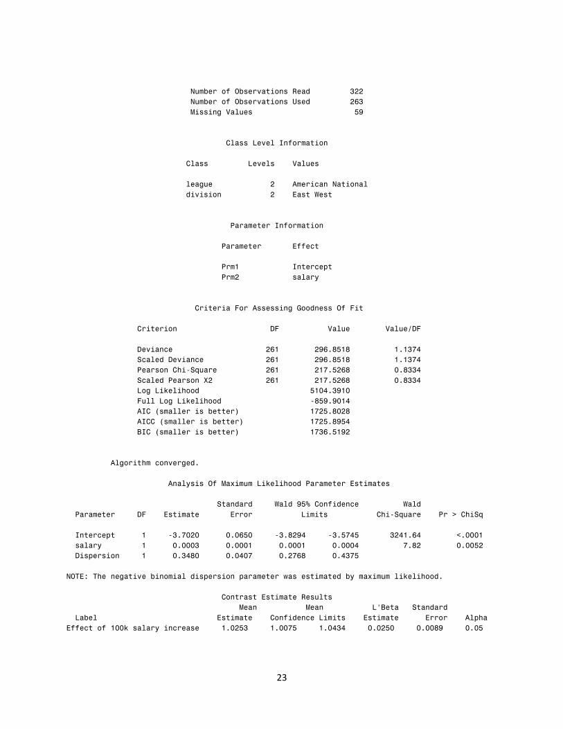
Here, we use some SAS code to create groups based on the predicted value (i.e., an

approximation to the mean of the conditional distribution). We then look at the distribution of the

mean of the predicted value in each interval, and the variance of the raw residuals. We see that

the mean of the distribution is in all cases less than the variance of the raw residuals. This is

another indication that the Poisson distribution is not the best choice for this problem.

22

data Pfitdata2;

set Pfitdata;

if 0<= predict <5 then group=1;

if 5<= predict <10 then group=2;

if 10<= predict < 15 then group=3;

if 15<= predict < 20 then group=4;

if 20<= predict then group=5;

run;

proc format;

value grpfmt 1="0 to 4.9" 2="5 to 9.9" 3="10 to 14.9"

4="15 to 19.9" 5="20 to Max";

run;

proc means data=Pfitdata2 n min max mean std var;

class group;

var predict resraw;

format group grpfmt.;

run;

group N Obs Variable N Minimum Maximum Mean Std Dev Variance

0 to 4.9 13 predict

resraw

13

13

3.2578916

-3.6719335

4.9212568

7.9021423

4.1868213

0.6593325

0.4976284

3.4251530

0.2476340

11.7316732

5 to 9.9 95 predict

resraw

95

95

5.0315488

-7.9171285

9.9696055

14.8172419

7.4209071

-0.2209071

1.4917644

4.6511984

2.2253609

21.6336467

10 to 14.9 81 predict

resraw

81

81

10.1005542

-13.9169213

14.9827472

20.8129702

12.5494485

0.1912922

1.5378169

8.1655403

2.3648810

66.6760486

15 to 19.9 60 predict

resraw

60

60

15.0114917

-15.4846933

19.9416355

20.2883934

16.9885310

-0.0218643

1.4100640

9.1883062

1.9882804

84.4249700

20 to Max 14 predict

resraw

14

14

20.3345690

-20.3773828

27.4575979

14.1047560

22.4834298

-0.1262870

2.2746223

9.7491252

5.1739064

95.0454412

We now change the distribution to a negative binomial.

ods graphics on;

proc genmod data=baseball plots = (predicted(clm));

class league division;

model no_home = salary / dist=negbin offset=log_atbat;

output out=nbfitdata p=predict resraw=resraw reschi=reschi;

estimate "Effect of 100k salary increase" salary 100 / est;

run;

ods graphics off;

Model Information

Data Set WORK.BASEBALL

Distribution Negative Binomial

Link Function Log

Dependent Variable no_home

Offset Variable log_atbat

23



Missing Values 59

Class Level Information

Class Levels Values

league 2 American National

division 2 East West

Parameter Information

Parameter Effect

Prm1 Intercept

Prm2 salary

Criteria For Assessing Goodness Of Fit

Criterion DF Value Value/DF

Deviance 261 296.8518 1.1374

Scaled Deviance 261 296.8518 1.1374

Pearson Chi-Square 261 217.5268 0.8334

Scaled Pearson X2 261 217.5268 0.8334

Log Likelihood 5104.3910

Full Log Likelihood -859.9014

AIC (smaller is better) 1725.8028

AICC (smaller is better) 1725.8954

BIC (smaller is better) 1736.5192

Algorithm converged.

Analysis Of Maximum Likelihood Parameter Estimates

Standard Wald 95% Confidence Wald

Parameter DF Estimate Error Limits Chi-Square Pr > ChiSq

Intercept 1 -3.7020 0.0650 -3.8294 -3.5745 3241.64 <.0001

salary 1 0.0003 0.0001 0.0001 0.0004 7.82 0.0052

Dispersion 1 0.3480 0.0407 0.2768 0.4375

NOTE: The negative binomial dispersion parameter was estimated by maximum likelihood.

Contrast Estimate Results

Mean Mean L'Beta Standard

Label Estimate Confidence Limits Estimate Error Alpha

Effect of 100k salary increase 1.0253 1.0075 1.0434 0.0250 0.0089 0.05

24

We now see that the scaled deviance divided by df is approximately 1.0, which is an

improvement over the previous model.

In this model, the predicted effect of a 100k increase in salary is predicted to be about a 2.5%

increase in home run production, with a wider Confidence Interval (CI = 0.75% to 4.3%).

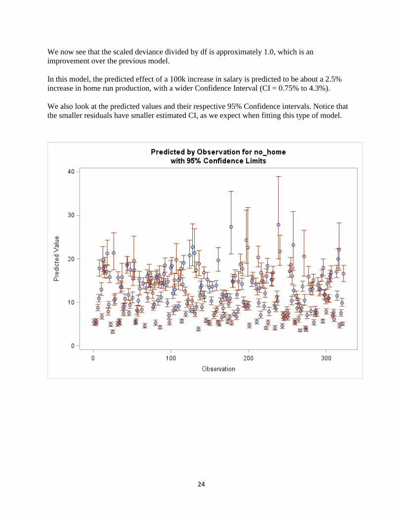
We also look at the predicted values and their respective 95% Confidence intervals. Notice that

the smaller residuals have smaller estimated CI, as we expect when fitting this type of model.

basic statistical and modeling procedures using saskwelch/b600/2015/b600...1 basic statistical and...

Documents