basics of computer networking - stony brooktom/robertazzi-basics-comp-net-11-28-11.pdf · basics of...
TRANSCRIPT

Basics of
Computer Networking
Thomas G. Robertazzi
Stony Brook University
September 19, 2011

To Marsha,
My Late Wife and Partner

ii Preface
Preface
Computer networking is a fascinating field that has interested many for quite a
few years. The purpose of this brief book is to give a general, non-mathematical,
introduction to the technology of networks. This includes discussions of types of
communication, many networking standards, popular protocols, venues where net-
working is important such as data centers, cloud computing and grid computing and
the most important civilian encryption algorithm, AES.
This brief book can be used in undergraduate and graduate networking courses
in universities or by the individual engineer, computer scientist or information tech-
nology professional. In universities it can be used in conjunction with more mathe-
matical modeling oriented texts.
I have learned a great deal about networking by teaching undergraduate and
graduate courses on the topic at Stony Brook. I am grateful to Dantong Yu of
Brookhaven National Laboratory for making me aware of many recent technological
developments. Thanks are also due to Brett Kurzman, my editor at Springer, for
supporting this brief book project. I would like to acknowledge the assistance in my
regular duties at the university of my department’s superb staff of Gail Giordano,
Carolyn Huggins, Rachel Ingrassia and Debbie Kloppenburg. I would also like to
thank Prad Mohanty and Tony Olivo for excellent computer support.
The validation of my writing efforts by my daughters Rachel and Deanna and
my good friend Sandy Pike means a lot. Finally I dedicate this brief book to the
memory of my late wife and partner, Marsha.
Thomas Robertazzi, Stony Brook NY, September 2011
Contents
1 Introduction to Networks 1
1.1 Introduction . . . . . . . . . . . . . . . . . . . . . . . . . . . . . . . . 1
1.2 Achieving Connectivity . . . . . . . . . . . . . . . . . . . . . . . . . . 2
1.2.1 Coaxial Cable . . . . . . . . . . . . . . . . . . . . . . . . . . . 2
1.2.2 Twisted Pair Wiring . . . . . . . . . . . . . . . . . . . . . . . 3
1.2.3 Fiber Optics . . . . . . . . . . . . . . . . . . . . . . . . . . . . 4
1.2.4 Microwave Line of Sight . . . . . . . . . . . . . . . . . . . . . 5
1.2.5 Satellites . . . . . . . . . . . . . . . . . . . . . . . . . . . . . . 5
1.2.6 Cellular Systems . . . . . . . . . . . . . . . . . . . . . . . . . 8
1.2.7 Ad Hoc Networks . . . . . . . . . . . . . . . . . . . . . . . . . 9
1.2.8 Wireless Sensor Networks . . . . . . . . . . . . . . . . . . . . 11
1.3 Multiplexing . . . . . . . . . . . . . . . . . . . . . . . . . . . . . . . . 12
1.3.1 Frequency Division Multiplexing (FDM) . . . . . . . . . . . . 12
1.3.2 Time Division Multiplexing (TDM) . . . . . . . . . . . . . . . 13
iii
iv Preface
1.3.3 Frequency Hopping . . . . . . . . . . . . . . . . . . . . . . . . 14
1.3.4 Direct Sequence Spread Spectrum . . . . . . . . . . . . . . . . 14
1.4 Circuit Switching Versus Packet Switching . . . . . . . . . . . . . . . 16
1.5 Layered Protocols . . . . . . . . . . . . . . . . . . . . . . . . . . . . . 18
2 Ethernet 23
2.1 Introduction . . . . . . . . . . . . . . . . . . . . . . . . . . . . . . . . 23
2.2 10 Mbps Ethernet . . . . . . . . . . . . . . . . . . . . . . . . . . . . . 24
2.3 Fast Ethernet . . . . . . . . . . . . . . . . . . . . . . . . . . . . . . . 28
2.4 Gigabit Ethernet . . . . . . . . . . . . . . . . . . . . . . . . . . . . . 30
2.5 10 Gigabit Ethernet . . . . . . . . . . . . . . . . . . . . . . . . . . . . 32
2.6 40/100 Gigabit Ethernet . . . . . . . . . . . . . . . . . . . . . . . . . 35
2.6.1 40/100 Gigabit Technology . . . . . . . . . . . . . . . . . . . . 35
2.7 Conclusion . . . . . . . . . . . . . . . . . . . . . . . . . . . . . . . . . 37
3 InfiniBand 39
3.1 Introduction . . . . . . . . . . . . . . . . . . . . . . . . . . . . . . . . 39
3.2 A First Look . . . . . . . . . . . . . . . . . . . . . . . . . . . . . . . 40
3.3 The InfiniBand Protocol . . . . . . . . . . . . . . . . . . . . . . . . . 41
3.4 InfiniBand for HPC . . . . . . . . . . . . . . . . . . . . . . . . . . . . 42
3.5 Conclusion . . . . . . . . . . . . . . . . . . . . . . . . . . . . . . . . . 44

Preface v
4 Wireless Networks 45
4.1 Introduction . . . . . . . . . . . . . . . . . . . . . . . . . . . . . . . . 45
4.2 802.11 WiFi . . . . . . . . . . . . . . . . . . . . . . . . . . . . . . . . 45
4.2.1 The Original 802.11 Standard . . . . . . . . . . . . . . . . . . 46
4.2.2 Other 802.11 Versions . . . . . . . . . . . . . . . . . . . . . . 48
4.3 802.15 Bluetooth . . . . . . . . . . . . . . . . . . . . . . . . . . . . . 51
4.3.1 Technically Speaking . . . . . . . . . . . . . . . . . . . . . . . 52
4.3.2 Ad Hoc Networking . . . . . . . . . . . . . . . . . . . . . . . . 53
4.3.3 Versions of Bluetooth . . . . . . . . . . . . . . . . . . . . . . . 53
4.3.4 802.15.4 Zigbee . . . . . . . . . . . . . . . . . . . . . . . . . . 54
4.3.5 802.15.6 Wireless Body Area Networks . . . . . . . . . . . . . 56
4.3.6 Bluetooth Security . . . . . . . . . . . . . . . . . . . . . . . . 57
4.4 802.16 Wireless MAN . . . . . . . . . . . . . . . . . . . . . . . . . . . 58
4.4.1 Introduction . . . . . . . . . . . . . . . . . . . . . . . . . . . . 58
4.4.2 The Original 802.16 Standard . . . . . . . . . . . . . . . . . . 59
4.4.3 More Recent 802.16 Standards . . . . . . . . . . . . . . . . . . 60
4.4.4 802.16j . . . . . . . . . . . . . . . . . . . . . . . . . . . . . . . 62
4.4.5 802.16m . . . . . . . . . . . . . . . . . . . . . . . . . . . . . . 63
4.5 LTE: Long Term Evolution . . . . . . . . . . . . . . . . . . . . . . . . 64
4.5.1 Introduction . . . . . . . . . . . . . . . . . . . . . . . . . . . . 64

vi Preface
4.5.2 LTE . . . . . . . . . . . . . . . . . . . . . . . . . . . . . . . . 65
4.5.3 LTE Advanced . . . . . . . . . . . . . . . . . . . . . . . . . . 66
5 Asynchronous Transfer Mode (ATM) 69
5.1 ATM (Asynchronous Transfer Mode) . . . . . . . . . . . . . . . . . . 69
5.1.1 Limitations of STM . . . . . . . . . . . . . . . . . . . . . . . . 70
5.1.2 ATM Features . . . . . . . . . . . . . . . . . . . . . . . . . . . 71
5.1.3 ATM Switching . . . . . . . . . . . . . . . . . . . . . . . . . . 75
6 Multiprotocol Label Switching (MPLS) 79
6.1 Introduction . . . . . . . . . . . . . . . . . . . . . . . . . . . . . . . . 79
6.2 Technical Details . . . . . . . . . . . . . . . . . . . . . . . . . . . . . 80
6.3 Traffic Engineering . . . . . . . . . . . . . . . . . . . . . . . . . . . . 83
6.4 Fault Management . . . . . . . . . . . . . . . . . . . . . . . . . . . . 84
6.5 GMPLS . . . . . . . . . . . . . . . . . . . . . . . . . . . . . . . . . . 85
7 SONET and WDM 87
7.1 SONET . . . . . . . . . . . . . . . . . . . . . . . . . . . . . . . . . . 87
7.1.1 SONET Architecture . . . . . . . . . . . . . . . . . . . . . . . 89
7.1.2 Self-Healing Rings . . . . . . . . . . . . . . . . . . . . . . . . 92
7.2 Wavelength Division Multiplexing (WDM) . . . . . . . . . . . . . . . 94
8 Grid and Cloud Computing 97
Preface vii
8.1 Introduction . . . . . . . . . . . . . . . . . . . . . . . . . . . . . . . . 97
8.2 Grids . . . . . . . . . . . . . . . . . . . . . . . . . . . . . . . . . . . . 97
8.3 Cloud Computing . . . . . . . . . . . . . . . . . . . . . . . . . . . . . 101
8.3.1 Tradeoffs for Cloud Computing . . . . . . . . . . . . . . . . . 102
9 Data Centers 105
9.1 Introduction . . . . . . . . . . . . . . . . . . . . . . . . . . . . . . . . 105
9.2 Data Centers . . . . . . . . . . . . . . . . . . . . . . . . . . . . . . . 106
9.2.1 Racks . . . . . . . . . . . . . . . . . . . . . . . . . . . . . . . 106
9.2.2 Networking Support . . . . . . . . . . . . . . . . . . . . . . . 106
9.2.3 Storage . . . . . . . . . . . . . . . . . . . . . . . . . . . . . . 108
9.2.4 Electrical and Cooling Support . . . . . . . . . . . . . . . . . 108
9.2.5 Management Support . . . . . . . . . . . . . . . . . . . . . . . 110
9.2.6 Ownership . . . . . . . . . . . . . . . . . . . . . . . . . . . . . 110
9.2.7 Security . . . . . . . . . . . . . . . . . . . . . . . . . . . . . . 110
10 Advanced Encryption Standard (AES) 111
10.1 Introduction . . . . . . . . . . . . . . . . . . . . . . . . . . . . . . . . 111
10.2 DES . . . . . . . . . . . . . . . . . . . . . . . . . . . . . . . . . . . . 112
10.3 Choosing AES . . . . . . . . . . . . . . . . . . . . . . . . . . . . . . . 112
10.4 AES Issues . . . . . . . . . . . . . . . . . . . . . . . . . . . . . . . . . 114
10.4.1 Security Aspect . . . . . . . . . . . . . . . . . . . . . . . . . . 114

viii Preface
10.4.2 Performance Aspect . . . . . . . . . . . . . . . . . . . . . . . 115
10.4.3 Intellectual Property Aspect . . . . . . . . . . . . . . . . . . . 116
10.4.4 Some Other Aspects . . . . . . . . . . . . . . . . . . . . . . . 116
11 Bibliography 119
12 Index 129

Chapter 1
Introduction to Networks
1.1 Introduction
There is something about technology that allows people and their computers to com-
municate with each other that makes networking a fascinating field, both technically
and intellectually.
What is a network? It is a collection of computers (nodes) and transmission
channels (links) that allow people to communicate over distances, large and small.
A Bluetooth personal area network may simply connect your home PC with its
peripherals. An undersea fiber optic cable may traverse an ocean. The Internet and
telephone networks span the globe.
Networking in particular has been a child of the late twentieth century. The
Internet has been developed over the past 40 years or so. The 1980’s and 1990’s saw
the birth and growth of local area networks, SONET fiber networks and ATM back-
bones. The 1990’s and the early years of the new century have seen the development
and expansion of WDM fiber multiplexing. New wireless standards continue to ap-
pear. Cloud computing and data centers are increasingly becoming a foundation of
today’s networking/computing world.
1

2 Chapter 1. Introduction to Networks
The book’s purpose is to give a concise overview of some major topics in net-
working. We now start with an introduction to the applied aspects of networking.
1.2 Achieving Connectivity
A variety of transmission methods, both wired and wireless, are available today to
provide connectivity between computers, networks, and people. Wired transmission
media include coaxial cable, twisted pair wiring and fiber optics. Wireless technology
includes microwave line of sight, satellites, cellular systems, ad hoc networks and
wireless sensor networks. We now review these media and technologies.
1.2.1 Coaxial Cable
This is the thick cable you may have in your house to connect your cable TV set up
box to the outside wiring plant. This type of cable has been around for many years
and is a mature technology. While still popular for cable TV systems today, it was
also a popular choice for wiring local area networks in the 1980s. It was used in the
wiring of the original 10 Mbps Ethernet.
A coaxial cable has four parts: a copper inner core, surrounded by insulating
material, surrounded by a metallic outer conductor; finally surrounded by a plastic
outer cover. Essentially in a coaxial cable, there are two wires (copper inner core
and outer conductor) with one geometrically inside the other. This configuration
reduces interference to/from the coaxial cable with respect to other nearby wires.
The bandwidth of a coaxial cable is on the order of 1 GHz. How many bits per
second can it carry? Modulation is used to match a digital stream to the spectrum
carrying ability of the cable. Depending on the efficiency of the modulation scheme
used, 1 bps requires anywhere from 1/14 to 4 Hz. For short distances, a coaxial
cable may use 8 bits/Hz or carry 8 Gbps.

Chapter 1. Introduction to Networks 3
There are also different types of coaxial cable. One with a 50 ohm termination
is used for digital transmissions. One with a 75 ohm termination is used for analog
transmissions or cable TV systems.
A word is in order on cable TV systems. Such networks are locally wired as tree
networks with the root node called the head end. At the head end, programming
is brought in by fiber or satellite. From the head end cables (and possibly fiber)
radiate out to homes. Amplifiers may be placed in this network when distances are
large.
For many years, cable TV companies were interested in providing two way ser-
vice. While early limited trials were generally not successful (except for Video on
Demand), more recently cable TV seems to have winners in broadband access to
the Internet and in carrying telephone traffic.
1.2.2 Twisted Pair Wiring
Coaxial cable is generally no longer used for wiring local area networks. One type
of replacement wiring has been twisted pair. Twisted pair wiring typically had
been previously used to wire phones to the telephone network. A twisted pair
consists of two wires twisted together over their length. The twisted geometry
reduces electromagnetic leakage (i.e. cross talk) with nearby wires. Twisted pairs
can run several kilometers without the need for amplifiers. The quality of a twisted
pair (carrying capacity) depends on the number of twists per inch.
About 1990, it became possible to send 10 Mbps (for Ethernet) over unshielded
twisted pair (UTP). Higher speeds are also possible if the cable and connector pa-
rameters are carefully implemented.
One type of unshielded twisted pair is category 3 UTP. It consists of four pairs
of twisted pair surrounded by a sheath. It has a bandwidth of 16 MHz. Many offices
used to be wired with category 3 wiring.

4 Chapter 1. Introduction to Networks
Category 5 UTP has more twists per inch. Thus, it has a higher bandwidth (100
MHz). Newer standards include category 6 versions (250 MHz or more) and category
7 versions (600 MHz or more). Category 8 at 1200 MHz is under development
(Wikipedia).
The fact that twisted pair is lighter and thinner than coaxial cable has speeded
its widespread acceptance.
1.2.3 Fiber Optics
Fiber optic cable consists of a silicon glass core that conducts light, rather than
electricity as in coaxial cables and twisted pair wiring. The core is surrounded by
cladding and then a plastic jacket.
Fiber optic cables have the highest data carrying capacity of any wired medium.
A typical fiber has a capacity of 50 Tbps (terabits per second or 50 × 1012 bits per
second). In fact, this data rate for years has been much higher than the speed at
which standard electronics could load the fiber. This mismatch between fiber and
nodal electronics speed has been called the electronic bottleneck. Decades ago the
situation was reversed, links were slow and nodes were relatively fast. This paradigm
shift has led to a redesign of protocols.
There are two major types of fiber: multi-mode and single mode. Pulse shapes
are more accurately preserved in single mode fiber, lending to a higher potential
data rate. However, the cost of multi-mode and single mode fiber is comparable.
The real difference in pricing is in the opto-electronics needed at each end of the
fiber. One of the reasons multi-mode fibers have a lower performance is dispersion.
Under dispersion, square digital pulses tend to spread out in time, thus lowering the
potential data rate. Special pulse shapes (such as hyperbolic cosines) called solitons,
that dispersion is minimized for, have been the subject of research.
Mechanical fiber connectors to connect two fibers can lose 10% of the light that

Chapter 1. Introduction to Networks 5
the fiber carries. Fusing two ends of the fiber results in a smaller attenuation.
Fiber optic cables today span continents and are laid across the bottom of oceans
between continents. They are also used by organizations to internally carry tele-
phone, data and video traffic.
1.2.4 Microwave Line of Sight
Microwave radio energy travels largely in straight lines. Thus, some network opera-
tors construct networks of tall towers kilometers apart and place microwave antennas
at different heights on each tower. While the advantage is that there is no need to
dig trenches for cables, the expense of tower construction and maintenance must be
taken into account.
1.2.5 Satellites
Arthur C. Clarke, the science fiction writer, made popular the concept of using
satellites as communication relays in the late 1940s. Satellites are now extensively
used for communication purposes. They fill certain technological niches very well:
providing connectivity to mobile users, for large area broadcasts and for communi-
cations for areas with poor infrastructure. The two main communication satellite
architectures are geostationary satellites and low earth orbit satellites (LEOS). Both
are now discussed.
Geostationary Satellites
You may recall from a physics course that a satellite in a low orbit (hundreds of
kilometers) around the equator seems to move against the sky. As its orbital altitude
increases, its apparent movement slows. At a certain altitude of approximately
36,000 km, it appears to stay in one spot in the sky, over the equator, 24 hours a

6 Chapter 1. Introduction to Networks
day. In reality, the satellite is moving around the earth but at the same angular
speed that the earth is rotating, giving the illusion that it is hovering in the sky.
This is very useful. For instance, a satellite TV service can install home antennas
that simply point to the spot in the sky where the satellite is located. Alternatively,
a geostationary satellite can broadcast a signal to a large area (its footprint) 24
hours a day.
By international agreement, geostationary satellites are placed 2 degrees apart
around the equator. Some locations are more economically preferable than others,
depending on which regions of the earth are under the location.
A typical geostationary satellite will have several dozen transponders (relay am-
plifiers), each with a bandwidth of 80 MHz (Tanenbaum 03). Such a satellite may
weigh several thousand kilograms and consume several kilowatts using solar panels.
The number of microwave frequency bands used have increased over the years
as the lower bands have become crowded and technology has improved. Frequency
bands include L (1.5/1.6 GHz), S (1.9/2.2 GHz), C (4/6 GHz), Ku (11/14 GHz)
and Ka (20/30 GHz) bands. Here the first number is the downlink band and the
second number is the uplink band. The actual bandwidth of a signal may vary from
about 15 MHz in the L band to several GHz in the Ka band (Tanenbaum 03).
It should be noted that extensive studies of satellite signal propagation under
different weather and atmospheric conditions have been conducted. Excess power
for overcoming rain attenuation is often budgeted above 11 GHz.
Low Earth Orbit Satellites
A more recent architecture is that of low earth orbit satellites. The most famous
such system was Iridium from Motorola. It received its name because the original
proposed 77 satellite network has the same number of satellites as the atomic number

Chapter 1. Introduction to Networks 7
North Pole
South Pole
PolarOrbit
Satellite
Earth
Figure 1.1: Low earth orbit satellites (LEOS) in polar orbits.
of the element Iridium. In fact, the actual system orbited had 66 satellites but the
system name Iridium was kept.
The purpose of Iridium was to provide a global cell phone service. One would
be able to use an Iridium phone anywhere in the world (even on the ocean or in
the Artic). Unfortunately, after spending five billion dollars to deploy the system,
talking on Iridium cost a dollar or more a minute while local terrestrial cell phone
service was under 25 cents a minute. While an effort was made to appeal to business
travelers, the system was not profitable and was sold and is now operated by a private
company.
Technologically though, the Iridium system is interesting. There are eleven satel-
lites in each of six polar orbits (passing over the North Pole, south to the South Pole
and back up to the North Pole, see Figure 1.1).

8 Chapter 1. Introduction to Networks
At any given time, several satellites are moving across the sky over any location
on earth. Using several dozen spot beams, the system can support almost a quarter
of a million conversations. Calls can be relayed from satellite to satellite.
It should be noted that when Iridium was hot, several competitors were proposed
but not built. One used a bent pipe architecture where a call to a satellite would
be beamed down from the same satellite to a ground station and then sent over the
terrestrial phone network rather than being relayed from satellite to satellite. This
was done in an effort to lower costs and simplify the design.
1.2.6 Cellular Systems
Starting around the early 1980s, cellular telephone systems which provide connectiv-
ity between mobile phones and the public switched telephone network were deployed.
In such systems, signals go from/to a cell phone to/from a local base station an-
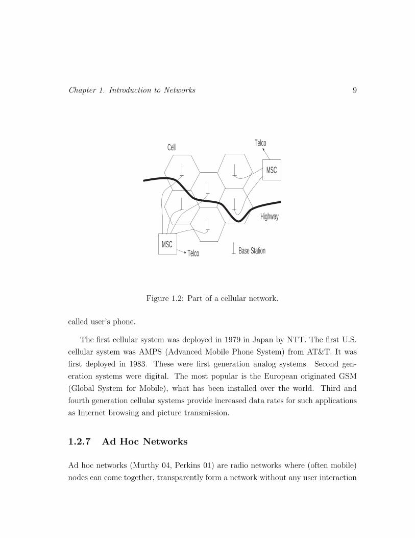
tenna which is hard wired into the public switched telephone network. Figure 1.2
illustrates such a system. A geographic region such as a city or suburb is divided
into geographic sub-regions called cells.
Base stations are shown at the center of cells. Nearby base stations are wired
into a switching computer (the mobile switching center or MSC) that provides a
path to the telephone network.
A cell phone making a call connects to the nearest base station (i.e., the base
station with the strongest signal). Base stations and cell phones measure and com-
municate received power levels. If one is driving and one approaches a new base
station, its signal will at some point become stronger than that of the original base
station one is connected to and the system will then perform a handoff. In a hand-
off, connectivity is changed from one base station to an adjacent one. Handoffs are
transparent, the talking user is not aware when one occurs.
Calls to a cell phone involve a paging like mechanism that activates (rings) the
Chapter 1. Introduction to Networks 9
MSC
MSC
Highway
Telco
Telco
Base Station
Cell
Figure 1.2: Part of a cellular network.
called user’s phone.
The first cellular system was deployed in 1979 in Japan by NTT. The first U.S.
cellular system was AMPS (Advanced Mobile Phone System) from AT&T. It was
first deployed in 1983. These were first generation analog systems. Second gen-
eration systems were digital. The most popular is the European originated GSM
(Global System for Mobile), what has been installed over the world. Third and
fourth generation cellular systems provide increased data rates for such applications
as Internet browsing and picture transmission.
1.2.7 Ad Hoc Networks
Ad hoc networks (Murthy 04, Perkins 01) are radio networks where (often mobile)
nodes can come together, transparently form a network without any user interaction

10 Chapter 1. Introduction to Networks
and maintain the network as long as the nodes are in range of each other and energy
supplies last (Rabaey 00, Mauve 01). In an ad hoc network messages hop from node
to node to reach an ultimate destination. For this reason ad hoc networks used to
be called multi-hop radio networks. In fact, because of the nonlinear dependence of
energy on transmission distance, the use of several small hops uses much less energy
than a single large hop, often by orders of magnitude.
Ad hoc network characteristics include multi-hop transmission, possibly mobility
and possibly limited energy to power the network nodes. Applications include mobile
networks, emergency networks, wireless sensor networks and ad hoc gatherings of
people, as at a convention center.
Routing is an important issue for ad hoc networks. Two major categories of
routing algorithms are topology based routing and position based routing. Topology
based routing uses information on current links to perform the routing. Position
based routing makes use of a knowledge of the geographic location of each node to
route. The position information may be acquired from a service such as the Global
Positioning System (GPS).
Topology based algorithms may be further divided into proactive and reactive
algorithms. Proactive algorithms use information on current paths as inputs to clas-
sical routing algorithms. However to keep this information current a large amount of
control message traffic is needed, even if a path is unused. This overhead problem is
exacerbated if there are many topology changes (say due to movement of the nodes).
On the other hand, reactive algorithms such as DSR, TORA and AODV maintain
routes only for paths currently in use to keep the amount of information and control
overhead more manageable. Still, more control traffic is generated if there are many
topology changes.
Position based routing does not require maintenance of routes, routing tables,
or generation of large amounts of control traffic other than information regarding

Chapter 1. Introduction to Networks 11
positions. “Geocasting” to a specific area can be simply implemented. A number of
heuristics can be used in implementing position based routing.
1.2.8 Wireless Sensor Networks
The integration of wireless, computer and sensor technology has the potential to
make possible networks of miniature elements that can acquire sensor data and
transmit the data to a human observer. Wireless sensor networks have received
attention from researchers in universities, government and industry because of their
promise to become a revolutionary technology and the technical challenges that must
be overcome to make this a reality. It is assumed that such wireless sensor networks
will use ad hoc radio networks to forward data in a multi-hop mode of operation.
Typical parameters for a wireless sensor unit (including computation and net-
working circuitry) include a size from 1 millimeter to 1 centimeter, a weight less
than 100 grams, cost less than one dollar and power consumption less than 100 mi-
crowatts (Shah 02). By way of contrast, a wireless personal area network Bluetooth
transceiver consumes more than a 1000 microwatts. A cubic millimeter wireless
sensor can store, with battery technology, 1 Joule allowing a 10 microwatt energy
consumption for 1 day (Kahn 00). Thus energy scavenging from light or vibration
has been proposed. Note also that data rates are often relatively low for sensor data
(100s bps to 100 Kbps).
Naturally, with these parameters, minimizing energy usage in wireless sensor
networks becomes important. While in some applications wireless sensor networks
may be needed for a day or less, there are many applications where a continuous
source of power is necessary. Moreover, communication is much more energy expen-
sive than computation. Sending one bit for a distance of 100 meters can take as
much energy as processing 3000 instructions on a micro-processor.
While military applications of wireless sensor networks are fairly obvious, there

12 Chapter 1. Introduction to Networks
are many potential scientific and civilian applications of wireless sensor networks.
Scientific applications include geophysical, environmental and planetary exploration.
One can imagine wireless sensor networks being used to investigate volcanoes, mea-
sure weather, monitor beach pollution or record planetary surface conditions.
Biomedical applications include applications such as glucose level monitoring and
retinal prosthesis (Schwiebert 01). Such applications are particularly demanding in
terms of manufacturing sensors that can survive in and not affect the human body.
Sensors can be placed in machines (where vibration can sometimes supply en-
ergy) such as rotating machines, semiconductor processing chambers, robots and
engines. Wireless sensors in engines could be used for pollution control telemetry.
Finally, among many potential applications, wireless sensors could be placed
in homes and buildings for climate control. Note that wiring a single sensor in
a building can cost several hundred dollars. Ultimately, wireless sensors could be
embedded in building materials.
1.3 Multiplexing
Multiplexing involves sending multiple signals over a single medium. Thomas Edison
invented a four to one telegraph multiplexer that allowed four telegraph signals
to be sent over one wire. The major forms of multiplexing for networking today
are frequency division multiplexing (FDM), time division multiplexing (TDM) and
spread spectrum. Each is now reviewed.
1.3.1 Frequency Division Multiplexing (FDM)
Here a portion of spectrum (i.e. band of frequencies) is reserved for each channel
(Figure 1.3(a)). All channels are transmitted simultaneously but a tunable filter at

Chapter 1. Introduction to Networks 13
slot 1 slot 2 slot 3 slot N slot 1 slot 2
Frame 1 Frame 2
FDM
TDM (a)
(b)
channel 1 channel 2 channel 3 channel Nfrequency
time
Figure 1.3: (a) Frequency division multiplexing, (b) Time division multiplexing.
the receiver only allows one channel at a time to be received. This is how AM, FM
and analog television signals are transmitted. Moreover, it is how distinct optical
signals are transmitted over a fiber using wavelength division multiplexing (WDM)
technology.
1.3.2 Time Division Multiplexing (TDM)
Time division multiplexing is a digital technology that, on a serial link, breaks
time into equi-duration slots (Figure 1.3(b)). A slot may hold a voice sample in a
telephone system or a packet in a packet switching system. A frame consists of N
slots. Frames, and thus slots, repeat. A telephone channel might use slot 14 of 24
slots in a frame during the length of a call, for instance.
Time division multiplexing is used in the second generation cellular system, GSM.
14 Chapter 1. Introduction to Networks
It is also used in digital telephone switches. Such switches in fact use electronic
devices called time slot interchangers that transfer voice samples from one slot to
another to accomplish switching.
1.3.3 Frequency Hopping
Frequency hopping is one form of spread spectrum technology and is typically used
on radio channels. The carrier (center) frequency of a transmission is pseudo-
randomly hopped among a number of frequencies. (Figure 1.4(a)). The hopping
is done in a deterministic, but random looking pattern that is known to both trans-
mitter and receiver. If the hopping pattern is known only to the transmitter and
receiver, one has good security. Frequency hopping also provides good interference
rejection. Multiple transmissions can be multiplexed in the same local region if each
uses a sufficiently different hopping pattern. Frequency hopping dates back to the
era of World War II.
1.3.4 Direct Sequence Spread Spectrum
This alternative spread spectrum technology uses exclusive or (xor) gates as scram-
blers and de-scramblers. (Figure 1.4(b)). At the transmitter data is fed into one
input of an xor gate and a pseudo-random key stream into the other input.
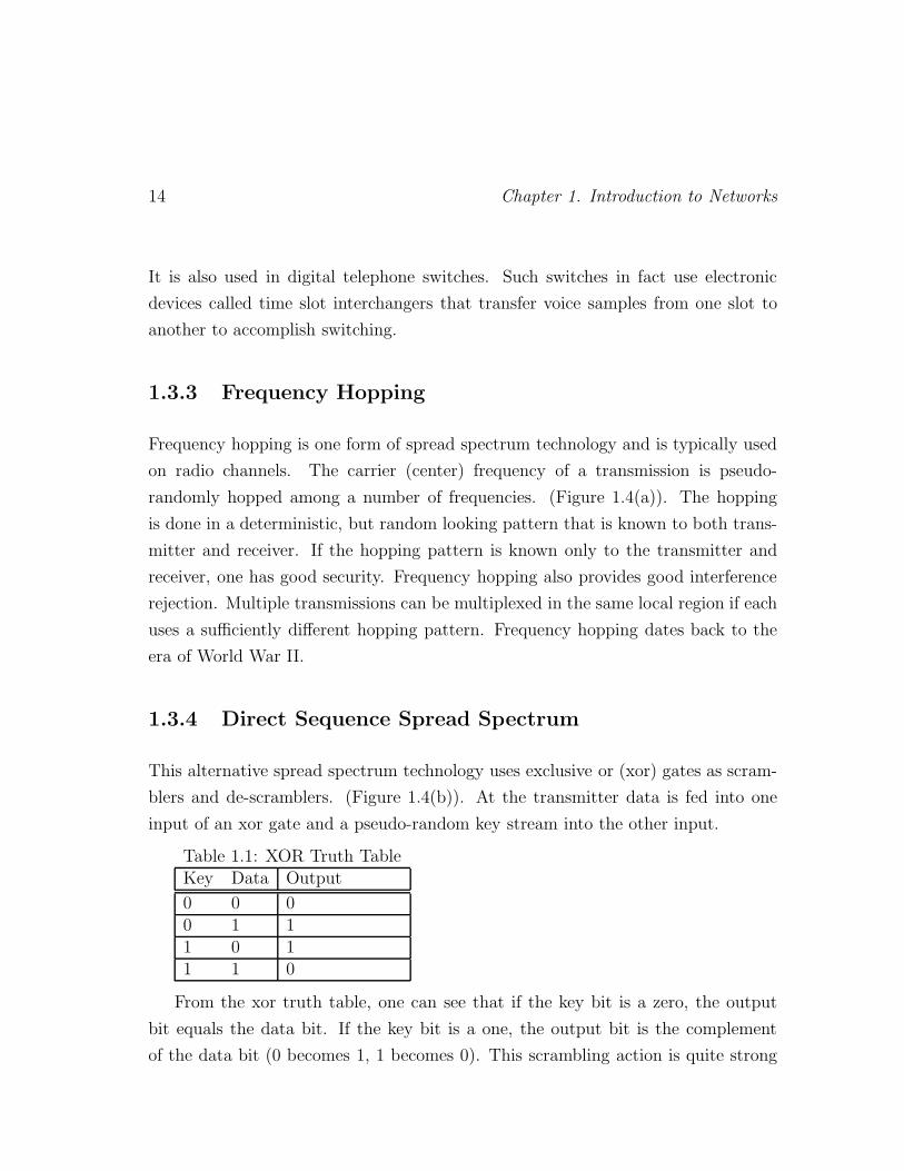
Table 1.1: XOR Truth TableKey Data Output
0 0 00 1 11 0 11 1 0
From the xor truth table, one can see that if the key bit is a zero, the output
bit equals the data bit. If the key bit is a one, the output bit is the complement
of the data bit (0 becomes 1, 1 becomes 0). This scrambling action is quite strong

Chapter 1. Introduction to Networks 15
f
f
f
f
1
2
3
4
time
Frequency Hopping
(a)
XOR
101
00
Key stream
XOR
101
00
Key stream
Channel
Transmitter Receiver
Direct Sequence
Data Data
00110 00110
(b)
Figure 1.4: (a) Frequency hopping spread spectrum, (b) Direct sequence spreadspectrum.

16 Chapter 1. Introduction to Networks
under the proper conditions. Unscrambling can be performed by an xor gate at the
receiver. The transmitter and receiver must use the same (synchronized) key stream
for this to work. Again, multiple transmissions can be multiplexed in a local region
if the key streams used for each transmission are sufficiently different.
1.4 Circuit Switching Versus Packet Switching
Two major architectures for networking and telecommunications are circuit switch-
ing and packet switching. Circuit switching is the older technology, going back to
the years following the invention of the telephone in the late 1800’s. As illustrated
in Figure 1.5(a), for a telephone network, when a call has to be made from node A
to node Z, a physical path with appropriate resources called a circuit is established.
Resources include link bandwidth and switching resources. Establishing a circuit
requires some set-up time before actual communication commences. Even if one
momentarily stops talking, the circuit is still in operation. When the call is fin-
ished, link and switching resources are released for use by other calls. If insufficient
resources are available to set up a call, the call is said to be blocked.
Packet switching was created during the 1960’s. A packet is a bundle of bits
consisting of header bits and payload bits. The header contains the source and des-
tination address, priority levels, error check bits and any other information that is
needed. The payload is the actual information (data) to be transported. However,
many packet switching systems have a maximum packet size. Thus, larger trans-
missions are split into many packets and the transmission is reconstituted at the
receiver.
The diagram of Figure 1.5(b) shows packets, possibly from the same transmis-
sion, taking multiple routes from node A to node Z. This is called datagram or
connectionless oriented service. Packets may indeed take different routes in this
type of service as nodal routing tables are updated periodically in the middle of a

Chapter 1. Introduction to Networks 17
(a)
(b)
circuit
A
Z
A
Z
Circuit Switching
Packet Switching
Packet
Figure 1.5: (a) Circuit switching, (b) Packet switching.
transmission.
A hybrid type of service is the use of virtual circuits or connection oriented
service. Here packets belonging to the same transmission are forced to take the
same serial path through the network. A virtual circuit has an identification number
which is used at nodes to continue the circuit along its preset path. As in circuit
switching, a virtual circuit needs to be set up prior to its use for communication.
That is, entries need to be made in routing tables implementing the virtual circuit.
An advantage of virtual circuit usage is that packets arrive at the destination in
the same order that they were sent. This avoids the need for buffers for reassembling
transmissions (reassembly buffers) that are needed when packets arriving at the
destination are not in order, as in datagram service. As we shall see, ATM, the high
speed packet switching technology used in Internet backbones, uses virtual circuits.

18 Chapter 1. Introduction to Networks
Packet switching is advantageous when traffic is bursty (occurs at irregular in-
tervals) and individual transmissions are short. It is a very efficient way of sharing
network transmissions when there are many such transmissions. Circuit switching
is not well suited for bursty and short transmissions. It is more efficacious when
transmissions are relatively long (to minimize set up time overhead) and provide a
constant traffic rate (to well utilize the dedicated circuit resource).
1.5 Layered Protocols
Protocols are the rules of operation of a network. A common way to engineer a
complex system is to break it into more manageable and coherent components.
Network protocols are often divided into layers in the layered protocol approach.
Figure 1.6 illustrates the generic OSI (open systems interconnection) protocol stack.
Proprietary protocols may have different names for the layers and/or a different layer
organization but pretty much all networking protocols have the same functionality.
Transmissions in a layered architecture (see Figure 1.6) move from the source’s
top layer (application), down the stack to the physical layer, through a physical
channel in a network, to the destination’s physical layer, up the destination stack to
the destination application layer. Note that any communication between peer layers
must move down one stack, across and up the receiver’s stack. It should also be
noted that if a transmission passes through an intermediate node, only some lower
layers (e.g., network, data link and physical) may be used at the intermediate nodes.
It is interesting that a packet moving down the source’s stack may have its header
grow as each layer may append information to the layer. At the destination, each
layer may remove information from the packet header, causing it to decrease in size
as it moves up the stack.
In a particular implementation, some layers may be larger and more complex
while others are relatively simple.

Chapter 1. Introduction to Networks 19
Application
Presentation
Session
Transport
Network
Data Link
Physical
Application
Presentation
Session
Transport
Network
Data Link
Physical
Node A Node Z
Figure 1.6: OSI protocol stack for a communicating source and destination.
In the following, we briefly discuss each layer.
Application Layer
Applications for networking include email, remote login, file transfer and the world-
wide web. But an application may also be more specialized, such as distributed
software to run a network of catalog company order depots.
Presentation Layer
This layer controls how information is formatted, such as on a screen (number of
lines, number of characters across).

20 Chapter 1. Introduction to Networks
Session Layer
This layer is important for managing a session, as in remote logins. In other cases,
this is not a concern.
Transport Layer
This layer can be thought of as an interface between the upper and lower layers.
More importantly, it is designed to give the impression to the layers above that they
are dealing with a reliable network, even though the layers below the transport layer
may not be perfectly reliable. For this reason, some think of the transport layer as
the most important layer.
Network Layer
The network layer manages multiple links. Its most important function is to do
routing. Routing involves selecting the best path for a circuit or packet stream.
Data Link Layer
Whereas, the network layer manages multiple link functions, a data link protocol
manages a single link. One of its potential functions is encryption, which can either
be done on a link by link basis (i.e. at the data link layer) or on an end to end basis
(i.e. at the transport layer) or both. End to end encryption is a more conservative
choice as one is never sure what type of sub-network a transmission may pass thru
and what its level of encryption, if any, is.

Chapter 1. Introduction to Networks 21
Physical Layer
The physical layer is concerned with the raw transmission of bits. Thus, it includes
engineering physical transmission media, modulation and de-modulation and radio
technology. Many communication engineers work on physical layer aspects of net-
works. Again, the physical layer of a protocol stack is the only layer that provides
actual direct connectivity to peer layers.
Introductory texts on networking usually discuss layered protocols in detail.

22 Chapter 1. Introduction to Networks

Chapter 2
Ethernet
2.1 Introduction
Local area networks (LANs) are networks that cover a small area as in a department
in a company or university. In the early 1980s, the three major local area networks
were Ethernet (IEEE standard 802.3), Token Ring (802.5 and used extensively by
IBM) and Token Bus (802.4, intended for manufacturing plants). However, over the
years, Ethernet (Tanenbaum 03) has become the most popular local area network
standard. While maintaining a low cost, it has gone through six versions, most ten
times faster than the previous version (10 Mbps, 100 Mbps, 1 Gbps, 10 Gbps, 40
Gbps, 100 Gbps).
Ethernet was invented at the Xerox Palo Alto Research Center (PARC) by Met-
calfe and Boggs, circa 1976. It is similar in spirit to the earlier Aloha radio protocol,
though the scale is smaller. IEEE’s 802.3 committee produced the first Ethernet
standard. Xerox never produced Ethernet commercially but other companies did.
In going from one Ethernet version to the next, the IEEE 802.3 committee sought
to make each version similar to the previous ones and to use existing technology. In
the following, we now discuss the various versions of Ethernet.
23

24 Chapter 2. Ethernet
Coaxial Cable
Computers
(a)
Hub
Computers
(b)
ToBackbone
Figure 2.1: Ethernet wiring using (a) coaxial cable and (b) hub topology.
2.2 10 Mbps Ethernet
Back in the 1980’s, Ethernet was originally wired using coaxial cable. As in Fig-
ure 2.1(a), a coaxial cable was snaked through the floor or ceiling and computers
attached to it along its length. The coaxial cable acted as a private radio channel
that each computer would monitor. If a station had a packet to send, it would send
it immediately if the channel was idle. If the station sensed the channel to be busy,
it would wait until the channel was free. In all of this, only one transmission can be
on the channel at one time.
A problem occurs if two or more stations sense the channel to be idle at about the
same time and attempt to transmit simultaneously. The packets overlap in the cable
and are garbled. This is a collision. The stations involved, using analog electronics,
can detect the collision, stop transmitting and reschedule their transmissions.

Chapter 2. Ethernet 25
Thus, the price one pays for this completely decentralized access protocol is the
presence of utilization lowering collisions. The protocol used goes by the name 1-
persistent CSMA/CD (Carrier Sense Multiple Access with Collision Detection). The
name is pretty much self-explanatory except that 1-persistent refers to the fact that
a station with a packet to send attempts this on an idle channel with a probability
of 1.0. In a CSMA/CD protocol, if the bit rate is 10 Mbps, the actual useful
information transport can be significantly less because of collisions (or occasional
idleness).
In the case of a collision, the rescheduling algorithm used is called Binary Expo-
nential Backoff. Under this protocol, two or more stations experiencing a collision
randomly reschedule over a time window with a default of 51 microseconds for a 500
meter network. If a station becomes involved in a second collision, it doubles its
window size and attempts again to randomly reschedule its transmission. Windows
may be doubled in size up to ten times. Once a packet is successfully transmit-
ted, the window size drops back to the default (smallest) value for that packet’s
station. Thus, this protocol at a station has no long term memory regarding past
transmissions.
Table 2.1: Ethernet Frame FormatField Length
Preamble 7 bytesFrame Delimiter 1 byteDestination Address 2 or 6 bytesSource Address 2 or 6 bytesData Length 2 bytesData up to 1500 bytesPad variableCRC Checksum 4 bytes
Table 2.1 above shows the fields in the 10 Mbp Ethernet frame. A frame is the
name for a packet at the data link layer. The preamble is for communication receiver
synchronization purposes. Addresses are either local (2 bytes) or global (6 bytes).

26 Chapter 2. Ethernet
Note that Ethernet addresses are different from IP addresses. Different amounts
of data can be accommodated up to 1500 bytes. Transmissions longer than 1500
bytes of data must be segmented into multiple packets. The pad field is used to
guarantee that the frame is at least 64 bytes in length (minimum frame size) if the
frame would be less than 64 bytes in length. Finally the checksum is based on CRC
error detecting coding.
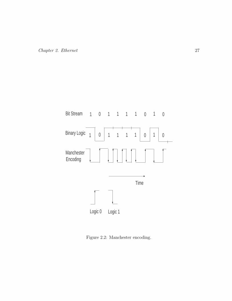
A problem with digital receivers is that they require many 0 to 1 and 1 to
0 transitions to properly lock onto a signal. But long runs of 1’s or 0’s are not
uncommon in data. To provide many transitions between logic levels, even if the
data has a long run of one logic level, 10 Mbps Ethernet uses Manchester encoding.
Referring to Figure 2.2, under Manchester encoding, if a logic 0 needs to be sent,
a transition is made for 0 to 1 (low to high voltage) and if a logic 1 needs to be
sent, the opposite transition is made for 1 to 0 (high to low voltage). The voltage
level makes a return to its original level at the end of a bit as necessary. Note that
the signaling rate is variable. That is, the number of transitions per second is twice
the data rate for long runs of a logic level and is equal to the data rate if the logic
level alternates. For this reason, Manchester encoding is said to have an efficiency
of 50%. More modern signaling codes, such as 4B5B, achieve a higher efficiency (see
Fast Ethernet below).
During the 1980s, Ethernets were wired with linear coaxial cables. Today hubs
are commonly used (Figure 2.1(b)). These are boxes (some smaller than a cigar
box) that computers tie into, in a star type wiring pattern, with the hub at the
center of the star.
A hub may internally have multiple cards, each of which have multiple external
Ethernet connections. A high speed (in the gigabits) proprietary bus interconnects
the cards. Cards may mimic a CSMA/CD Ethernet with collisions (shared hub) or
use buffers at each input (switched hub). In a switched hub, multiple packets may
be received simultaneously without collisions, raising throughput.
Chapter 2. Ethernet 27
1 0 1 1 1 1 0 1 0
1 0 1 1 1 1 10 0
Time
Bit Stream
Binary Logic
ManchesterEncoding
Logic 0 Logic 1
Figure 2.2: Manchester encoding.

28 Chapter 2. Ethernet
The next table (Table 2.2) illustrates Ethernet wiring. In 10 Base5, the 10 stands
for 10 Mbps and the 5 for the 500 meter maximum size. Used in the early 1980s,
10 Base5 used vampire taps which would puncture the cable. Also at the time, 10
Base2 used T junctions and BNC connectors as wiring hardware. Today, 10 Base-T
is the most common wiring solution for 10 Mbps Ethernet. Fiber optics, 10 Base-F,
is only intended for runs between buildings, but a higher data rate protocol would
probably be used today for this purpose.
Table 2.2: Original Ethernet WiringCable Type Maximum Size
10Base5 Thick Coax 500 m10Base2 Thin Coax 200 m10Base-T Twisted Pair 100 m10Base-F Fiber Optics 2 km
2.3 Fast Ethernet
As the original 10 Mbps Ethernet became popular and the years passed, traffic
on Ethernet networks continued to grow. To maintain performance, network ad-
ministrators were forced to segment Ethernet networks into smaller networks (each
handling a smaller number of computers) connected by a spaghetti-like arrangement
of repeaters, bridges and routers. In 1992, IEEE assigned the 802.3 committee the
task of developing a faster local area network protocol.
The committee agreed on a 100 Mbps protocol that would incorporate as much
of the existing Ethernet protocol/technology as possible to gain acceptance and so
that they could move quickly. The resulting protocol, IEEE 802.3u, was called Fast
Ethernet.
Fast Ethernet is only implemented with hubs, in a star topology (Figure 2.1(b)).
There are three major wiring options (Table 2.3).

Chapter 2. Ethernet 29
Table 2.3: Fast Ethernet WiringCable Type Maximum Size
100Base-T4 Twisted Pair 100 m100Base-TX Twisted Pair 100 m100Base-FX Fiber Optics 2 km
The original Ethernet has a data rate of 10 Mbps and a maximum signaling
rate of 20 MHz (recall that the Manchester encoding used was 50% efficient). Fast
Ethernet 100 Base-T4 with its data rate of 100 Mbps has a signaling speed of 25
MHz, not 200 MHz. How is this accomplished?
Fast Ethernet 100 Base-T4 actually uses four twisted pairs per cable. Three
twisted pairs carry signals from its hub to a PC. Each of the three twisted pairs
uses ternary (not binary) signaling using 3 logic levels. Thus, one of 3x3x3=27
symbols can be sent at once. Only 16 symbols are used though, which is equivalent
to sending 4 bits at once. With 25 MHz clocking 25 MHz x 4 bits yields a data rate
of 100 Mbps. The channel from the PC to hub operates at 33 MHz. For most PC
applications, an asymmetrical connection with more capacity from hub to PC for
downloads is acceptable. Category 3 or 5 unshielded twisted pair wiring is used for
100 Base-T4.
An alternative to 100 Base-T4 is 100 Base-TX. This uses two twisted pairs, with
100 Mbps in each direction. However, 100 Base-T4 has a signaling rate of only 125
MHz. It accomplishes this using 4B5B (Four Bit Five Bit) encoding rather than
Manchester encoding. Under 4B5B, every four bits is mapped into five bits in such
a way that there are many transitions for digital receivers to lock onto, irrespective
of the actual data stream. Since four bits are mapped into five bits, 4B5B is 80%
efficient. Thus, 125 MHz times 0.8 yields 100 Mbps.
Finally, 100 Base-FX uses two strands of the lower performing multimode fiber.
It has 100 Mbps in both directions and is for runs (say between buildings) of up to
2 km.

30 Chapter 2. Ethernet
It should be noted that Fast Ethernet uses the signaling method for twisted
pair (for 100 Base-TX) and fiber (100 Base-FX) borrowed from FDDI. The FDDI
protocol was a 100 Mbps token ring protocol used as a backbone in the 1980’s.
To maintain channel efficiency (utilization) at 100 Mbps, versus the original 10
Mbps, the maximum network size of Fast Ethernet is about ten times smaller than
that of the original Ethernet.
2.4 Gigabit Ethernet
The ever growing amount of network traffic brought on by the growth of applica-
tions and more powerful computers motivated a revised, faster version of Ethernet.
Approved in 1998, the next version of Ethernet operates at 1000 Mbps or 1 Gbps
and is known as Gigabit Ethernet, or 802.3z. As much as possible, the Ethernet
committee sought to utilize existing Ethernet features.
Gigabit Ethernet wiring is either between two computers directly or, as is more
common, in a star topology with a hub or switch in the center of the star. In
this connection, it is appropriate to say something about the distinction between a
hub and switch. A shared medium hub uses the established CSMA/CD protocol
so collisions can occur. At most, one attached station can successfully transmit
through the hub at a time, as one would expect with CSMA/CD. The half duplex
Gigabit Ethernet mode uses shared medium hubs.
A switch on the other hand, does not use CSMA/CD. Rather, the use of buffers
means multiple attached stations may send and receive distinct communications
to/from the switch at the same time. The use of multiple simultaneous transmissions
means that switch throughput is substantially greater than that of a single input line.
Level 2 switches are usually implemented in software, level 3 switches implement
routing functions in hardware (Stallings 02). Full duplex Gigabit Ethernet most
often uses switches.

Chapter 2. Ethernet 31
In terms of wiring, Gigabit Ethernet has two fiber optic options (1000 Base-
SX and 1000 Base-LX), a copper option (1000 Base-CX) and a twisted pair option
(1000-Base T).
The Gigabit Ethernet fiber option deserves some comment. It makes use of
8B10B encoding, which is similar in its operation to Fast Ethernet’s 4B5B. Under
8B10B, eight bits (1 byte) are mapped into 10 bits. The extra redundancy this
involves allows each 10 bits not to have an excessive number of bits of the same type
in a row or too many bits of one type in each of 10 bits. Thus, there are sufficient
transitions from 1 to 0 and 0 to 1 or the data stream even if the data has a long run
of 1s and 0s.
Gigabit Ethernet using twisted pair uses five logic levels on each wire. Four of
the logic levels convey data and the fifth is for control signaling. With four data
logic levels, two bits are communicated at once or eight bits over all four wires at a
time. Thus the signaling rate is 1 Gbps/8 or 125 MHz.
In terms of utilization under CSMA/CD operation, if the maximum segment size
had been reduced by a factor of 10 as was done in going from the original Ethernet
to Fast Ethernet, only very small gigabit networks could have been supported. To
compensate for the ten times increase in data rate relative to Fast Ethernet, the
minimum frame size for Gigabit Ethernet was increased (by a factor of eight) to
512 bytes from Fast Ethernet’s 512 bits (see Robertazzi 07 for a discussion of the
Ethernet equation that governs this).
Another technique that helps Gigabit Ethernet’s efficiency is frame bursting.
Under frame bursting, a series of frames are sent in a single burst.
Gigabit Ethernet’s range is at least 500 meters for most of the fiber options and
about 200 meters for twisted pair (Tanenbaum 03, Stallings 02).

32 Chapter 2. Ethernet
2.5 10 Gigabit Ethernet
Considering the improvement in Ethernet data rate over the years, it is not too
surprising that a 10 Gbps Ethernet was developed (Siwamogsatham 99, Vaughan-
Nichols 02). Continuing the increases in data rate by a factor of ten that have
characterized the Ethernet standards, 10 Gbps (or 10,000 Mbps) Ethernet is ten
times faster than Gigabit Ethernet. Applications include backbones, campus size
networks and metropolitan and wide area networks. This latter application is aided
by the fact that the 10 Gbps data rate is comparable with a basic SONET fiber
optic transmission standard rate. In fact, 10 Gbps Ethernet will be a competitor to
ATM high speed packet switching technology. See the following chapters for more
information on ATM and SONET.
There are eight implementations of 10 Gbps Ethernet. It can use four transceiver
types (one four wavelength parallel system and three serial systems with a number
of multimode and single mode fiber options). Like earlier versions of Ethernet, it
uses CRC error coding. It operates in full duplex non-CSMA/CD mode. It can go
more than 40 km via single mode fiber.
To lower the speed at which the MAC (Media Access Control) layer processes
the data stream, the MAC operates in parallel on four 2.5 Gbps streams (lanes). As
illustrated in Figure 2.3, bytes in an arriving 10 Gbps serial transmission are placed
in parallel in the four lanes.
There is a 12 byte Inter Packet Gap (IPG) which is the minimum gap between
packets. Normally, it would not be easy to predict the ending byte lane of the
previous packet, so it would be difficult to determine the starting lane of the next
transmission. The solution is to have a starting byte in a packet always occupy lane
0. The IPG is found using a pad (add in extra 1 to 3 bytes), a shrink (subtract 1 to
3 bytes) or through combination averaging (average of 12 bytes achieved through a
combination of pads and shrinks). Note that padding introduces extra overhead in

Chapter 2. Ethernet 33
12345
1
2
3
4
5 Lane 0
Lane 1
Lane 2
Lane 3
bytes
Figure 2.3: Four parallel lanes for 10 Gigabit Ethernet.
some implementations.
In terms of the protocol stack, this can be visualized as in Fig. 2.4.
The PCS, PMA and PMD sub-layers use parallel lanes for processing. In terms
of the sub-layers, they are:
Reconciliation: Command translator that maps terminology and commands in
MAC into electrical format appropriate for physical layer.
PCS: Physical Coding Sublayer.
PMA: Physical Medium Attachment (at transmitter serialize code groups into
bit stream, at receiver synchronization for data decoding).
PMD: Physical Medium Dependent (includes amplification, modulation, wave
shaping).
MDI: Medium Dependent Interface (i.e., connector).

34 Chapter 2. Ethernet
Reconcilation
Higher Layers
MAC Client
MAC
10 Gbps
OSI
Data Link
Physical
PCS
PMA
PMD
Medium
10 GMIIInterface
MDI
Figure 2.4: Protocol stack for 10 Gbps Ethernet.

Chapter 2. Ethernet 35
2.6 40/100 Gigabit Ethernet
Over the years Ethernet has been attractive to users because of its relatively low cost,
robustness and its ability to provide an interoperable network service. Users have
also liked the wide vendor availability of Ethernet related products. However even
with the release of gigabit and 10 Gbps Ethernet demand for bandwidth continued
to grow. Network equipment shipments can grow at a 17% a year rate. Internet
traffic grows at 75-125% a year. Computer performance doubles every 24 months.
A 2008 projection was that within four years 40 Gbps would be needed.
One of the applications driving this growth is the increasing use of data centers
(see the latter chapter on this topic). These facilities house server farms for hosting
web services and cloud computing services. Projections indicate a need for 100 Gbps
of data transfer capacity from switch to switch. Also 100 Gbps will have applications
between buildings, within campuses and for metropolitan area networks (MAN) and
wide area networks (WAN).
In July 2006 a committee was convened to explore increasing the data rate of
Ethernet beyond 10 Gbps. In 2010 standards for 40 Gbps and 100 Gbps Ethernet
were approved. This discussion is based on (D’Ambrosia 2008, Nowell 2007).
2.6.1 40/100 Gigabit Technology
In implementing 40 and 100 gigabit Ethernet some of the objectives are:
· MAC (medium access control) data rates of 40 and 100 gigabit per second.
· Full duplex is only supported (i.e. two way communication).
· Maintain the existing minimum and maximum frame length.
· Use the current frame format and MAC layer.

36 Chapter 2. Ethernet
MAC ClientMAC Control (optional)
MACReconciliation
PCSFEC (option)
PMAPMD
AN (option)
Medium
40 Gbps 100 Gbps
MDI
PCSFEC (option)
PMAPMD
AN (option)
MediumMDI
Figure 2.5: 40 and 100 Gbps Ethernet protocol functions
· Optical transport network (OTN) support.
A variety of transmission media can carry 40 and 100 gigabit Ethernet as Table
2.4 illustrates.
Table 2.4: 40/100 Gbps Ethernet40 Gbps 100 Gbps
≥ 10 km Single Mode Fiber ≥ 40 km Single-Mode Fiber≥ 100 m Multi-mode Fiber ≥ 10 km Single Mode Fiber≥ 10 m Copper cable ≥ 100 m Multi-mode Fiber≥ 1 m Backplane ≥ 10 m Copper Cable
Figure 2.5 illustrates the protocol stack for 40 and 100 gigabit Ethernet. In
the figure one has the physical coding sublayer (PCS), the forward error correction
sublayer (FEC), physical medium attachment sublayer (PMA), physical medium
dependent sublayer (PMD) and the auto-negotiation sublayer (AN). Here also MDI
is the medium dependent interface or the connector.

Chapter 2. Ethernet 37
In the physical coding sublayer 64B/66B coding is used, mapping 64 bits into
66 bits to provide enough transitions between 0 and 1 for digital receivers. As in 10
gigabit Ethernet, the concept of parallel lanes is used in 40 and 100 gigabit Ethernet.
A 66 bit block is distributed in round robin fashion on the PCS lanes. Specifically
for 40 gigabit Ethernet there are 4 PCS lanes that support 1 2 or 4 channels or
wavelengths. For 100 gigabit Ethernet there are 20 PCS lanes that support 1, 2, 4,
5, 10, or 20 channels or wavelengths. As an example, a 100 gigabit Ethernet may
use 5 parallel wavelengths over a fiber, each carrying 20 Gbps.
Created PCS lanes can be multiplexed into any interface width that is supported.
There is a unique lane marker for each PCS lane which is inserted perioidically.
Bandwidth for the lane marker comes from periodically deleting the inter-packet
gap (IPG) in a lane. All bits in the same lane follow the same physical path no
matter how multiplexing is done.
The receiver reassembles the PCS lanes by demultiplexing bits and also realigns
the PCS lanes taking into account the skewness of the lanes. Advantages of this
include the fact that all encoding, deskew and scrambling functions are implemented
on a CMOS device located on the host and there is minimal bit processing execept
for using an optical module for multiplexing.
Finally, clocking takes place at 1/64th of the data rate (625 MHz for 40 gigabits
and 1.5625 GHz for 100 gigabits). More information on 40 and 100 gigabit Ethernet
can be found on www.ethernetalliance.org
2.7 Conclusion
For thirty years Ethernet has continually transformed itself by way of higher data
rates to meet increasing demand for networking services. It will be interesting to
see what the future holds.

38 Chapter 2. Ethernet

Chapter 3
InfiniBand
3.1 Introduction
Data centers, facilities housing thousands of PCs, have become increasingly im-
portant to for hosting web services, such as Google, cloud computing and hosting
virtualized services. Data centers are also important for high performance comput-
ing (HPC) facilities which turn the power of thousands of PCs loose on difficult but
important scientific and engineering computational problems. Data centers are an
impressive technological wonder, with their energy consumption being an important
issue affecting their location and cost of operation.
“InfiniBand,” is a widely used interconnect used in high performance data cen-
ters to connect the thousands of PCs to each other. The following discussion is
based on the more extensive treatment in (Grun 10). The product started to be
offered in 1999. Often InfiniBand transfers data directly from the memory of one
computer to the memory of another without going through the computer’s operating
systems. This is referred to as “RDMA” or Remote Direct Memory Access. This
is an extension of Direct Memory Access (DMA) used in PCs. In DMA a DMA
engine (controller) allows memory access without involving the CPU processor. Off-
39

40 Chapter 3. InfiniBand
loading this function to the DMA engine makes for a more efficient use of the CPU.
The difference between RDMA and DMA is that RDMA is done between remote
(separate or distant) machines whereas DMA is done on a single machine.
One of the simplifying features of InfiniBand is that it provides a “messaging
service” that applications can directly access. This compares to byte stream oriented
TCP/IP over Ethernet, which is byte oriented rather than message oriented.
3.2 A First Look
The message service of InfiniBand is easy to use. It can allow communication from
an application to other applications or processes or to gain access to storage. In using
the messaging service the operating system is not needed. Instead an application
directly access the messaging service rather than one of the server’s communication
resources.
InfiniBand “creates” a channel application. Applications making use of the ser-
vice can either be kernel1 applications (such as file systems) or in user space. All
of InfiniBand is geared towards supporting this top-down messaging service. Chan-
nels serve as pipes (i.e. connections) between disjoint virtual address spaces. These
could also be disjoint physical address spaces (that is distinct servers separated by
distance).
Queue Pairs
The end points of a channel are the send and receive queueus. This is also known
as a queue pair. When an application requires one or more connections more Queue
1A kernel is the most basic part of most operating systems. It connects applications to dataprocessing in the computer’s hardware. Kernel address space is used exclusively by the kernel,kernel extensions and most device drivers while user space is where the user applications resideand work.

Chapter 3. InfiniBand 41
Pairs (QP’s) are generated. The Queue Pair maps directly into the virtual address
spaces of each application. This idea is called “channel I/O.”
Transfer Semantics
There are two ways in which data can be transferred in InfiniBand:
· SEND/RECEIVE: The application on the receiver side provides a data struc-
ture for received messages. The data structure is pre-posted on the receiver queue.
Actually the sending side doesn’t “see” the buffers or the data structure on the
receiver side. The sending side just SENDS one or more messages and the receiver
side RECEIVES them.
· RDMA READ/RDMA WRITE: The steps are as follows:
(a) A buffer is registered in the receiver side application’s virtual address space
by the receiver side application.
(b)Control of the buffer is passed to the sending side by the receiver.
(c)The sending side uses the RDMA READ or RDMA WRITE operations to
either read or write data in that buffer.
3.3 The InfiniBand Protocol
InfiniBand messages may be up to 231 bytes. Messages are partitioned (segmented)
into packets by the InfiniBand hardware. The packet size used is selected to make
the best use of network bandwidth. InfiniBand switches and routers are used for
transmitting packets through InfiniBand.
The generic OSI protocol stack layers that correspond to the InfiniBand messag-
ing service is illustrated in the accompanying figure. Here “SW” stands for software.

42 Chapter 3. InfiniBand
Application
InfiniBandMessagingService
SW TransportInterface
Transport
Network
Link
Physical
RDMA MessageTransport Service
Figure 3.1: InfiniBand Equivalency to OSI Protocol Stack (after Grun 10)
An InfiniBand switch is similar in theory to other types of common switches but
is adapted to InfiniBand performance and cost goals. InfiniBand switches use cut
through switching for better performance. Under cut through switching a node can
start forwarding a packet before it is completely received by the node. InfiniBand
link layer flow control is employed so during standard operation packets are not
dropped. Ethernet has more loss than InfiniBand. It should be mentioned that, as
opposed to switches, InfiniBand routers are not widely used.
Software for InfiniBand is made up of upper layer protocols (ULPs) and libraries.
Mid-layer functions support the ULPs. There are hardware specific data drivers.
3.4 InfiniBand for HPC
The Message Passing Interface (MPI) is the leading standard and model for parallel
system communication. Why use MPI? It offers a communication service to the dis-
tributed processes making up an HPC (High Performance Computing) application.

Chapter 3. InfiniBand 43
In fact MPI middleware2 is used by InfiniBand. The MPI middleware in InfiniBand
is allowed to communicate between machines in a cluster without the involvement of
the CPUs in the cluster. The copy avoidance3 architecture and stack bypass feature
of InfiniBand provide extremely low application to application delay (latency), high
bandwidth and low CPU loading.
Some other InfiniBand options, particularly for use with storage, include:
SDP (Socket Direct Protocol): This allows a socket application to use the Infini-
Band network without changing the application.
SCSI RDMA Protocol: The Small Computer System Interface (SCSI) make
possible data transfer between computers and peripheral devices. It is commonly
pronounced “scuzzy.” InfiniBand can enable a SCSI system to use RDMA semantics4
to connect to storage.
IP over InfiniBand: This makes it possible for an application hosted by Infini-
Band to communicate to the outside word using IP based semantics.
NFS-RDMA: This is the Network File System over RDMA. The NFS is a widely
used file system for use with TCP/IP networks. It allows a computer acting as a
client to access files over a network in much the same way it access local files. It
was originally developed by SUN Microsystems.
Lustre Support: Lustre is a large scale (massive) file system for use in large
cluster computers. Lustre can support tens of thousands of computers, petabytes of
storage and hundreds of gigabytes/second of input/output throughput. It is used
in both supercomputers and data centers (Wikipedia). It is available under GNU
General Purpose License (GPL). The name “Lustre” comes from the words Linux
2Middleware is software which connects application software to the operating system. Sometypes of middleware are eventually incorporated into newer versions of operating systems. Anexample of this migration is TCP/IP.
3Copy avoidance methods use less copying of data to memory by the operating system leadingto higher data transfer rates. Zero copy methods make no copies.
4“Semantics” is the meaning of computer instructions – “syntax” is their format.

44 Chapter 3. InfiniBand
and Cluster.
3.5 Conclusion
InfiniBand competes with Ethernet to provide high performance interconnects for
HPC systems. Traditionally HPC was the primary market for InfiniBand. However
it is finding a new role in cloud computing environments including those used for
financial services where low latency and high bandwidth are important considera-
tions.

Chapter 4
Wireless Networks
4.1 Introduction
Wireless technology has unique capabilities to service mobile nodes and establish
network infrastructure without wiring. Wireless technology has received an increas-
ing amount of R&D attention in recent years. In this section, the popular 802.11
WiFi, 802.15 Bluetooth, 802.16 WIMAX and LTE standards are discussed.
4.2 802.11 WiFi
The IEEE 802.11 standards (Goldberg 97, Kapp 02, La Maire 96) have a history
that goes back a number of years. The original standard was 802.11 (circa 1997).
However, it was not that big a marketing success because of a relatively low data rate
and relatively high cost. Future standardized products (such as 802.11b, 802.11a,
and 802.11g) were more capable and much more successful. We will start by dis-
cussing the original 802.11 standard. All 802.11 versions are meant to be wireless
local area networks with ranges of several hundred feet.
45

46 Chapter 4. Wireless Networks
AccessPoint
S3S4
AccessPoint
S5S6
S1
S2
Ad HocMode
Backbone Network
Figure 4.1: Modes of operation for 802.11 protocol.
4.2.1 The Original 802.11 Standard
The original 802.11 standard can operate in two modes (see the accompanying fig-
ure). In one mode, 802.11 capable stations connect to access points that are wired
into a backbone. The other mode, ad hoc mode, allows one 802.11 capable station
to connect directly to another without using an access point.
The 802.11 standard uses part of the ISM (Industrial, Scientific and Medical)
band. The ISM band allows unlicensed use, unlike much other spectrum. It has been
popular for garage door openers, cordless telephones, and other consumer electronic
devices. The ISM band includes 902-928 MHz, 2.400-2.4835 GHz and 5.725-5.850
GHz. The original 802.11 standard used the 2.400-2.4835 GHz band.
In fact, infrared wireless local area networks have also been built but are not used
today on a large scale. Using pulse position modulation (PPM), they can support

Chapter 4. Wireless Networks 47
at least a 1 to 2 Mbps data rate.
The 802.11 standard can use either direct sequence or frequency hopping spread
spectrum. Frequency hopping systems hop between 79 frequencies in the U.S. and
Europe and 23 frequencies in Japan. Direct sequence achieves data rates of 2 Mbps
while frequency hopping can send data at 1 or 2 Mbps in the original 802.11 standard.
Because of the spatial expanse of wireless networks, the type of collision detection
used in Ethernet would not work. Consider two stations, station 1 and station 2,
that are not in range of each other. However, both are in range of station 3. Since
the first two stations are not in range of each other, they could both transmit to
station 3 simultaneously upon detecting an idle channel in their local geographic
region. When both transmissions reach station 3, a collision results (i.e., overlapped
garbled signals). This situation is called the hidden node problem (Tanenbaum 03).
To avoid this problem, instead of using CSMA/CD, 802.11 uses CDMA/CA
(Carrier Sense Multiple Access with Collision Avoidance). To see how this works,
consider only station 1 and station 3. Station 1 issues a RTS (request to send)
message to station 3 which includes the source and destination addresses, the data
type and other information. Station 3, upon receiving the RTS and wishing to receive
a communication from station 1, issues a CTS (clear to send) message signaling
station 1 to transmit. In the context of the previous example, station 2 would hear
the CTS and not transmit to station 3 while station 1 is transmitting. Note RTS’s
may still collide but this would be handled by rescheduled transmissions.
The 802.11 protocol also supports asynchronous and time critical traffic as well
as power management to prolong battery life.
The second figure of this chapter shows the timing of events in an 802.11 channel.
Here after the medium becomes idle a series of delays called spaces are used to set up
a priority system between acknowledgements, time critical traffic and asynchronous
traffic. An interframe space is an IFS.

48 Chapter 4. Wireless Networks
Busy Medium
SIFS
PIFS
DIFS
Next Frame
Contention Window
RandomBackoff
Time
Figure 4.2: Timing of 802.11 between two transmissions.
Now, after the SIFS (short interframe space) acknowledgements can be transmit-
ted. After the PIFS (point coordination interframe space) time critical traffic can
be transmitted. Finally, after the DIFS (distributed coordination interface space)
asynchronous or data traffic can be sent. Thus, acknowledgements have the highest
priority, time critical traffic has the next highest priority, and asynchronous traffic
has the lowest priority.
The original 802.11 standard had an optional encryption protocol called WEP
(wired equivalent privacy). A European competitor to 802.11 is HIPERLAN (and
HIPERLAN2). Finally, note that wireless protocols are more complex than wired
protocols, for local area network and other environments.
4.2.2 Other 802.11 Versions
Since the original 802.11, a number of improved versions were developed and have
become available. The original 802.11 version itself did not sell well as the price
and performance was not that appealing. The four general variations are 802.11b,

Chapter 4. Wireless Networks 49
802.11a, 802.11g and 802.11n. Each is now briefly discussed. See Kapp 02, Vaughan-
Nichols 06, Poole 07 and Kuran 07 for discussions. There are 800 million new 802.11
devices sold every year (Wikipedia). More U.S. households use WiFi for a home LAN
rather than Ethernet.
802.11b: This 1999 version first made WiFi popular. It operates at a maximum
of 11 Mbps at a range of 100-150 feet and 2 Mbps at 250-300 feet. Data rate decreases
with distance to 1 Mbps and then goes to zero. If Wired Equivalent Privacy is used
with encryption, the actual useful data rate drops by 50%.
The 802.11b signal is in the 2.4 GHz band. It can operate either using direct
sequence spread spectrum, frequency hopping or infrared. Direct sequence is very
popular and infrared is mostly not in use.
802.11a In spite of the name, 802.11a was developed after 802.11b. It operates
at 54 Mbps in the UNI (Unlicensed Infrastructure Band):
Table 4.1: UNI BandsName Band
UNI-1 5.2 GHzUNI-2 5.7 GHzUNI-3 5.8 GHz
There is some disagreement in the technical literature as to whether 802.11b or
802.11a has the larger range.
802.11g: Sometimes 802.11g is known as 802.11b extended. Initial versions were
at 22 Mbps, later versions were at 54 Mbps. Using 802.11g and methods to increase
thruput can offer data rates of 100-125 Mbps (Kuran 07).
802.11n: A committee was formed to create a higher rate version of 802.11
(Poole 07a) in 2004. Two years later there was early industry agreement on the
features of 802.11n. The most significant feature of 802.11n is the use of MIMO
(multiple input multiple output) antenna technology. Normally when a radio signal
is transmitted from a transmitter to a receiver, the receiver may receive multiple
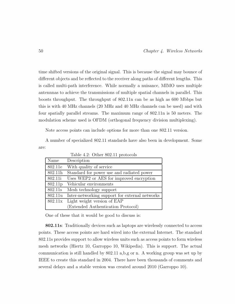
50 Chapter 4. Wireless Networks
time shifted versions of the original signal. This is because the signal may bounce of
different objects and be reflected to the receiver along paths of different lengths. This
is called multi-path interference. While normally a nuisance, MIMO uses multiple
antennnas to achieve the transmissions of multiple spatial channels in parallel. This
boosts throughput. The throughput of 802.11n can be as high as 600 Mbbps but
this is with 40 MHz channels (20 MHz and 40 MHz channels can be used) and with
four spatially parallel streams. The maximum range of 802.11n is 50 meters. The
modulation scheme used is OFDM (orthogonal frequency division multiplexing).
Note access points can include options for more than one 802.11 version.
A number of specialized 802.11 standards have also been in development. Some
are:
Table 4.2: Other 802.11 protocolsName Description
802.11e With quality of service802.11h Standard for power use and radiated power802.11i Uses WEP2 or AES for improved encryption802.11p Vehicular environments802.11s Mesh technology support802.11u Inter-networking support for external networks802.11x Light weight version of EAP
(Extended Authentication Protocol)
One of these that it would be good to discuss is:
802.11s: Traditionally devices such as laptops are wirelessly connected to access
points. These access points are hard wired into the external Internet. The standard
802.11s provides support to allow wireless units such as access points to form wireless
mesh networks (Hiertz 10, Garroppo 10, Wikipedia). This is support. The actual
communication is still handled by 802.11 a,b,g or n. A working group was set up by
IEEE to create this standard in 2004. There have been thousands of comments and
several delays and a stable version was created around 2010 (Garroppo 10).

Chapter 4. Wireless Networks 51
In 802.11s the basic unit is a “mesh station” which is networked with other mesh
stations statically or in an ad hoc fashion. A collection of mesh stations and the
networked links between them is a mesh basic service set (MBSS). A mesh station
can be a gateway or bridge to an external network in which case it can be referred
to as a mesh portal.
Techniques are used in 802.11s that hide the multi-hop nature of the mesh from
the upper layers of the protocol stack. It seeks to be functionally equivalent to a
broadcast Ethernet.
There is a mandatory path (route) selection algorithm and a mandatory link
metric for inter-operability reasons but other algorithms/metrics can be utilized.
Unicast, multicast and broadcast transmission of frames is supported in 802.11s.
Mesh stations can detect each other using passive scanning (noticing beacon frames)
or active scanning (sending probe frames). Stations may user single transceivers (on
one frequency) or multi-transceivers (on different frequencies). Finally most 802.11s
meshes will use the 802.11u standard for authentication of users.
A word is in order on 802.11 security. A user requires some sophistication to
prevent snooping by others. For instance, security features on shipped products are
often disabled by default. Williams reports that many corporate users are not using
or misusing WEP. These are media articles on people driving by in vans tapping
into private networks. The 2001 article by Williams describes a series of security
weaknesses in 802.11b. Some in the wireless LAN industry feel if one uses accepted
security practices along with 802.11 features, security is acceptable.
4.3 802.15 Bluetooth
The original goal of Bluetooth technology, standardized as IEEE 802.15, is to provide
an inexpensive, low power chip that can fit into any electronic device and use ad
hoc radio networking to make the device part of a network. For instance, if your

52 Chapter 4. Wireless Networks
PC, printer, monitor and speakers were Bluetooth enabled, most of the rat’s nest of
wiring under a desk top would be eliminated. Bluetooth chips could also be placed
in PDAs, headsets, etc.
Work on Bluetooth started in 1997. Five initial corporate supporters (Erickson,
Nokia, IBM, Toshiba and Intel) grew to a more than a thousand adopters by 2000.
The name Bluetooth comes from the Viking King of Denmark, Harald Blatand, who
unified Norway and Denmark in the 10th Century (Haartsen 00).
4.3.1 Technically Speaking
Bluetooth had a number of design goals. As related in Haartsen 00, among these
are:
• System should function globally
• Ad hoc networking
• Support for data and voice
• Inexpensive, minature and low power radio transceiver
The original Bluetooth operates in the 2.4 GHz ISM band (see the previous
section’s discussion of the ISM band). It uses frequency hopping spread spectrum
(79 hopping channels, 1600 hops/sec). Time is divided into 625 microsecond slots
with one packet fitting in one slot. The data rate is 1 Mbps. The range is 10 meters,
making Bluetooth a personal area network (PAN).
Two types of connections are possible with Bluetooth. First, SCO links (Syn-
chronous Connection Oriented) are symmetrical, point to point, circuit switched
voice connections. Secondly, ACL links (Asynchronous Connectionless) are asym-
metrical or symmetrical, point to multipoint, packet switched connections for data.
A number of features of Bluetooth are designed to make possible good interfer-

Chapter 4. Wireless Networks 53
ence immunity. One is the use of high rate frequency hopping with short packets.
There is an option to use error correction and a fast acting automatic repeat request
scheme using error detection. Finally, voice encoding that is not that susceptible to
bit errors is used.
4.3.2 Ad Hoc Networking
Two or more Bluetooth nodes form a piconet in sharing a frequency hopping channel.
One node will become a master node to supervise networking. The other nodes are
slaves. Not only may roles change but roles are lost when a connection is finished.
All SCO and ACL traffic is scheduled by the master node (Haartsen 00). The
master node allocates capacity for SCO links by reserving slots. Polling is used by
ACL links. That is, the master node prompts each slave node in turn to see if it has
data to transmit (see Schwartz 87 for a detailed discussion of polling). Slave node
clocks are synchronized to the master node’s clock.
There is a maximum of 8 active nodes on a single piconet (others may be parked
in an inactive state). As the number of nodes increases, throughput (i.e. useful
information flow) decreases. To mitigate this problem, several piconets with inde-
pendent but overlapping coverage can form a “scatternet”. Each piconet that is
part of a scatternet uses a separate pseudo-random frequency hopping sequence.
The scatternet approach results in a very small decrease in throughput. Note that a
node can be on several piconets in a scatternet. Moreover, it may be a master node
on some piconets and a slave node on other piconets.
4.3.3 Versions of Bluetooth
There are four versions of Bluetooth as illustrated in the table.

54 Chapter 4. Wireless Networks
Table 4.3: Bluetooth versions [Wikipedia]Version Data Rate Max Application Thruput
Version 1.2 1 Mbps 0.7 MbpsVersion 2.0+ 3 Mbps 2.1 MbpsVersion 3.0+ maybe 24 Mbps 2.1 MbpsVersion 4.0 maybe 24 Mbps 2.1 Mbps
The indicated 24 Mbps data rate in the table is not transmitted over Bluetooth
itself. Rather it is transmitted over a parallel 802.11 link whose operation is nego-
tiated using Bluetooth. Version 4.0 includes protocols for (a) classic Bluetooth, (b)
Bluetooth high-speed and (c) Bluetooth low energy.
There was some effort that was not realized to make an 802.15 variant ultra
wide band (UWB) standard for Bluetooth (Linde 11). Ultra wide band technology
is a short range radio technology that spreads the communication spectrum over an
unusually wide band of spectrum. It can have low energy requirements.
4.3.4 802.15.4 Zigbee
In actuality, the original Bluetooth faced some problems in gaining acceptance. The
rapid growth of 802.11 technology and its pricing had not given Bluetooth a price
advantage on certain applications (Zheng 04). Also, Bluetooth is more complex than
its original design goal as an attempt was made to have it serve more applications
and supply quality of service. There is also some question on the scalability of
scatternets (Liu 03).
Two planned successors to the original 802.15 Bluetooth standard were 802.15.3a
for high rate ultra wideband (UWB) wireless personal area networks (WPAN) and
802.15.4 for low rate, low power WPANs. In this section, the low data rate extension
of Bluetooth is discussed.
A great many applications could benefit from a low data rate Bluetooth standard
(Zheng 04). Among these are home, factory and warehouse automation. These are

Chapter 4. Wireless Networks 55
applications for monitoring involving safety, the health field and the environment.
The use of low data rate Bluetooth for precision asset location and situation aware-
ness could take place for emergency services and inventory tracking. Finally, there
are potential entertainment applications including interactive toys and games.
Zigbee can operate either in the 2.4 GHz ISM band (available worldwide), the
ISM 868 MHz band (Europe) and the ISM 915 MHz band (North America). Twenty-
seven channels are defined for 802.15.4 as indicated below.
Table 4.4: Zigbee ChannelsNo. of Channels Data Rate Band
16 channels 250 kbps 2.4 GHz10 channels 40 kbps 915 MHz1 channel 20 kbps 868 MHz
Zigbee, like Bluetooth, has a range of 10 meters. Communication can take place
from a device to a coordinator, a coordinator to a device or between stations of the
same type (i.e. peer to peer) in a multi-hop mode of operation. An 802.15.4 network
can have up to 64,000 devices in terms of address space. Zigbee topology includes
a one hop star or the use of multi-hopping for connectivity beyond 10 meters.
In beacon enabled mode, the coordinator periodically broadcasts beacons to
synchronize the devices it is connected to and for other functions. In non-beacon
enabled mode, beacons are not broadcast periodically by the coordinator. Rather,
if a device requests beacons, the coordinator will transmit a beacon directly to the
device (Zheng 04). A loss of beacons can be used to detect link or node failures.
It is critical for certain applications to minimize Zigbee coordinator and device
energy usage. Some of these applications will be battery powered where batteries
will not be (practically or economically) replaceable.
The majority of power savings functions in 802.15.4 involve beacon-enabled
mode. In direct data transmissions between coordinators and devices, the transceivers
are only on 1/64 of the duration of a packetized superframe (i.e. collection of slots).

56 Chapter 4. Wireless Networks
A small CSMA/CD backoff duration, and brief warm-up times for transceivers are
also used to minimize power usage in 802.15.4.
Three security levels are available in 802.15.4. The lowest level is None Security
mode which is suitable if the upper layers provide security or security is not im-
portant. An access control list is used in the second level of security to allow only
authorized devices to access data. The Advanced Encryption Standard (AES) is
used in the highest, third security level.
Zigbee is built on an IEEE 802.15.4 foundation. While it is widely used in
applications involving metering it is not suitable for industrial applications with real
time requirements. Two industry standards also built on 802.15.4 are WirelesHART
and ISA100 (Yang 10). They emphasize real time and co-existence functionality.
4.3.5 802.15.6 Wireless Body Area Networks
Wireless body are networks (WBAN) are networks that can collect and transmit data
from different parts of the human body, possibly to remote sites (Kwak 10, Latre
11). Applications include medicine, finding lost items, data file transfer, gaming
(sensors can collect data on body part movement) and social networking (for instance
exchanging electronic business cards by simply shaking hands).
Medicine may be the biggest application of wireless body area networks. An
obvious application is to collect vital patient data and forward it to a remote site for
processing and diagnosis. This could be used for myocardial infarctions, and also for
diseases involving cancer, asthma, the neural system and the gastrointestinal tract
(Kwak 10).
Work on the IEEE 802.15.6 standard is an attempt to standardize networking
for wireless body area networks.
As of about 2010, 802.15.6 provides three physical (PHY) layer specifications

Chapter 4. Wireless Networks 57
(Kwak 10). The use of each depends on the type of application need:
1) Narrowband PHY: This physical layer handles radio transceiver activation and
de-activation, data transmission and receiving and clear channel assessment within
the current channel
2) Ultra Wideband PHY: This has a low and high band. There are eleven
potential channels of 499.2 MHz bandwidth each. The low band consists of channels
1 through 3 and the high band consists of channels 4 through 11. Channel 2 has a
center frequency of 3.9936 GHz and channel 7 has a center frequency of 7.9872 GHz.
Channel 2 and channel 7 are “mandatory” channel, other channels do not have to
be used. Typical data rates are 0.5 to 10 Mbps.
Ultra wideband transceivers are relatively simple.
3) Human Body Communication PHY: This has two frequency bands of 4 MHz
bandwidth and center frequencies of 16 MHz and 27 MHz. Both bands can be used
in the US, Korea and Japan. The 27 MHz band can be used in Europe.
A super-frame 1 structure is used by 802.15.6. Beacon periods (of the same
length as a super-frame) bound each super-frame. Boundaries of the beacon period
are selected by the hub station which is thereby allocating time slots.
Like Zigbee, with 802.16.6 there are security options for (a) unsecured commu-
nication (b) authentication only and (3) authentication and encryption.
4.3.6 Bluetooth Security
Bluetooth has been is use for about 10 years. Hackers and researchers have dis-
covered several security weaknesses during this time in Bluetooth enabled devices
(Dunning 10). In fact most Bluetooth attacks are not detected and are more local-
ized than Internet attacks so that they do not get the same amount of attention from
1A super-frame is a sequential concatenation of frames that repeats periodically.
58 Chapter 4. Wireless Networks
the public. It should also be noted that mobile and embedded Bluetooth devices
that receive attacks have few or no security features.
Dunning (Dunning 10) holds that one should use Bluetooth if proper security is
in place.
Most of the susceptibility of Bluetooth devices to attacks comes from lax default
security settings, a lack of understanding on the part of Bluetooth device owners
of security practice and deficient software development. One is safe from most
Bluetooth attacks if security settings are correctly configured.
Bluetooth has a few weaknesses that are inherent (Dunning 10):
• Wireless data can be (locally) intercepted.
• No third party can verify addresses, names and classes as on the Internet.
• Many devices can’t be patched so any weaknesses remain as long as they are
in use.
While Bluetooth threats will probably increase, the key to making them less
effective is a better understanding of their potential.
4.4 802.16 Wireless MAN
4.4.1 Introduction
While wireless connectivity is very convenient, 802.11 and 802.15 have somewhat
limited ranges (hundreds of feet and ten meters, respectively). A third wireless
standard is IEEE 802.16 (Ahmadi 09, Bacioccola 10, Eklund 02, Papapanagiotou 09,
Peters 09, Tanenbaum 03). It defines how a base station may provide connectivity to
computers in buildings up to several kilometers distant, or more recently, to mobile
users. A home or business owner may install an antenna that allows him or her

Chapter 4. Wireless Networks 59
broadband Internet connectivity while bypassing telephone or cable company wired
services. A mobile user’s laptop or cell phone may also achieve connectivity using
802.16.
4.4.2 The Original 802.16 Standard
Standard efforts on 802.16 began in 1999 and the original standard was published
in April 2001. The original standard was only for fixed location users.
The original 802.16 operates in the 10-66 GHz band to make possible a large
bandwidth and thus data rate. Precipitation can be a problem on this band so
forward error correction (Reed Solomon) coding is used. There is also an option for
the use of CRC coding. Radio at 10-66 GHz is directional so base stations can have
several antennas, each covering a different geographic sector.
The original 802.16 standard calls for the use of either time division duplexing
(TDD: base station and user antenna share a single channel divided into time slots
but do not transmit concurrently) or frequency division duplexing (FDD: separate
channels, sometimes transmit concurrently). Note that in TDD there is a variable
upstream/downstream capacity allocation via time slot assignment.
These types of modulation are used in the original 802.16 depending on distance:
Table 4.5: 802.16 Modulation FormatsDistance Modulation Bits per Symbol No. of Waveforms
Small Distance QAM-64 6 bits/symbol 64Medium Distance QAM-16 4 bits/symbol 16Large Distance QPSK 2 bits/symbol 4
In general, a digital modulation scheme encodes a symbol as one of a number of
possible amplitudes and phase shifts. For instance, QAM-64 has 64 combinations
of amplitude and phase shifts so the so the equivalent of 6 bits (26 = 64 ) can be
transmitted per symbol. As distance increases, it is harder to distinguish between

60 Chapter 4. Wireless Networks
the 64 combinations due to noise and channel effects so that fewer, more distinctive
combinations are used (16 for QAM-16 and then 4 for QPSK) with corresponding
lower bit/symbol rate. Note that if X MHz of spectrum is available, the data rates
are 6X Mbps for QAM-64, 4X Mbps for QAM-16 and 2X Mbps for QPSK.
In terms of security, mutual authorization using RSA public key cryptography
and X.509 certificates is specified in the original standard.
A variety of downstream traffic can be supported in connection-oriented mode.
The four supported classes are:
• Constant bit rate.
• Real time variable bit rate.
• Non-real time variable bit rate.
• Best effort.
The physical and data link protocol layers for 802.16 appear in the third figure
of this chapter.
The service specific convergence sublayer interfaces to the network layer and
is similar to the LLC (Logical Link Control) layer in older 802 standards. This
includes interfacing for ATM (ATM convergence sublayer) and IPv4, IPv6, Ethernet
and VLAN (packet convergence sublayer). The channel is supervised by the MAC
sublayer common part. Security (encryption, key management) is the responsibility
of the security sublayer.
4.4.3 More Recent 802.16 Standards
Since the original 2001 802.16 standard, there have been a number of improved
802.16 standards developed. For instance, the 802.16e standard of 2005 allowed
connectivity to mobile users.

Chapter 4. Wireless Networks 61
Service Specific Convergence Sublayer
MAC Sublayer Common Part
Security Sublayer
Transmission Convergence Sublayer
Physical Medium Dependent Sublayer
(QAM-64, QAM-16 and QPSK)
DataLinkLayer
PhysicalLayer
Figure 4.3: Protocol stack for the 802.16 standard.
Flexibility is a key feature of the 802.16 standardization effort. Several parts in
fact are optional. To be more specific, the standards deal largely with the physical
(PHY) and media access control (MAC) layers only and do not specify upper layer
signaling and the network architecture. This was a major reason that the WIMAX
forum was established in 2001 (www.wimaxforum.org). The WIMAX forum seeks
to enable conformity and inter-operability. The accompanying table illustrates some
of the 802.16 standards.
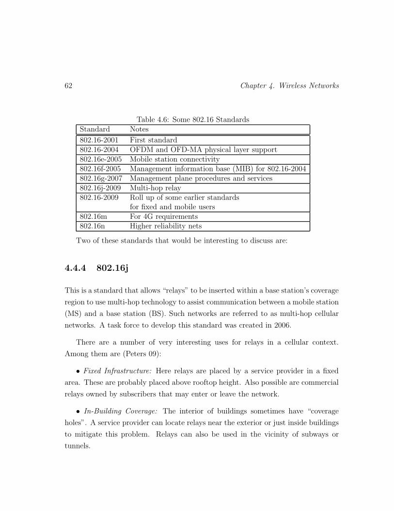
62 Chapter 4. Wireless Networks
Table 4.6: Some 802.16 StandardsStandard Notes
802.16-2001 First standard802.16-2004 OFDM and OFD-MA physical layer support802.16e-2005 Mobile station connectivity802.16f-2005 Management information base (MIB) for 802.16-2004802.16g-2007 Management plane procedures and services802.16j-2009 Multi-hop relay802.16-2009 Roll up of some earlier standards
for fixed and mobile users802.16m For 4G requirements802.16n Higher reliability nets
Two of these standards that would be interesting to discuss are:
4.4.4 802.16j
This is a standard that allows “relays” to be inserted within a base station’s coverage
region to use multi-hop technology to assist communication between a mobile station
(MS) and a base station (BS). Such networks are referred to as multi-hop cellular
networks. A task force to develop this standard was created in 2006.
There are a number of very interesting uses for relays in a cellular context.
Among them are (Peters 09):
• Fixed Infrastructure: Here relays are placed by a service provider in a fixed
area. These are probably placed above rooftop height. Also possible are commercial
relays owned by subscribers that may enter or leave the network.
• In-Building Coverage: The interior of buildings sometimes have “coverage
holes”. A service provider can locate relays near the exterior or just inside buildings
to mitigate this problem. Relays can also be used in the vicinity of subways or
tunnels.

Chapter 4. Wireless Networks 63
• Transient Coverage: Relays can be used to provide additional connectivity for
large and dense groups of people meeting in temporary situations. Relays in this
context can allow some traffic to be sent to base stations in adjacent cells. Relays
can also be used to maintain coverage in case of base station damage.
• Vehicular Coverage: This use includes buses and trains. Design of such relay
systems is a challenging problem as a mobile subscriber may hear signals both form
the relay and a base station. In general a relay transmits on both the uplink and
the downlink.
4.4.5 802.16m
The 802.16m standard will be considered for global 4G cellular network standard-
ization (i.e. IMT-Advanced). The goal of 802.16m is to make use of 802.16-2009
and 802.16j-2009 to create a capable air interface and to support legacy equipment.
The 802.16m standard introduces (Bacioccola 10):
• Femto Cell Support: Femto cells are small cells for the small office home office
(SOHO) environment. The femto cell base station is connected to the Internet
through a standard wired connection.
• Self-Organizing Networks: The purpose is to provide self organizing network
functionality to allow automatic configuration of base station parameters. The
amount of functionality should increase with more standards work.
• Self-Optimization Procedures: These allow a tuning of base station performance
parameters based on processing self-organizing network measurement data.
The physical layer of 802.16m uses OFDMA (Orthogonal Frequency Division
Multiple Access) and is to work in licensed bands under 6 GHz. Data rates for
802.16m are 100 Mbps for mobile users and 1 Gbps for fixed users.
A diagram of the 802.16m data and control plane appears in the accompanying

64 Chapter 4. Wireless Networks
Resource
Controland
Management
Functions
Convergence
Sublayer
CS SAP
MAC SAP
MAC Functions
Security Sublayer
Physical Layer (PHY)
PHY SAP
MAC Common Part Sublayer
M
A
C
P
H
Y
Figure 4.4: The IEEE 802.16m data and control plane.
figure.
4.5 LTE: Long Term Evolution
4.5.1 Introduction
Long Term Evolution or “LTE” is a process to create a new air interface for cell
phones by the 3rd Generation Partnership Project (3GPP). However LTE can also be
considered to be a system consisting of architecture and protocols and performance
goals.
When cell phones first came into use in the early 1980’s these “1st generation”
phones were analog based. Second generation phones were digital. Third and fourth
generations have increasing data rates allowing new services such as web surfing.
Some people call LTE a 3.9 technology in that it is almost but not quite 4th gener-

Chapter 4. Wireless Networks 65
ation technology. But the more recent “LTE Advanced” is a 4th generation system.
The initial proposal for LTE came from NTT DoCoMO of Japan. Began first as
a study item, the technical requirements of LTE were agreed to in 2005. The first
working LTE service for the public was in Stockholm and Oslo in 2009. A number
of carriers publicized plans, starting in 2009, to transform their networks into LTE
networks. These efforts began in 2010. Finally, LTE Advanced was submitted as a
candidate system that is fourth generation to ITU-T (International Telecommuni-
cations Union - Standardization Sector). The plan was for this to be finalized by
3GPP in 2011 (Wikipedia).
4.5.2 LTE
The goals of LTE include (Poole 07b, Rinne 10) reduced latency, higher data rates
for customers, better system capacity and coverage and a lower cost of operation.
Some important LTE features include (Rinne 10, Akyildiz 10):
• A flat IP oriented network architecture using distributed servers.
• In LTE, base stations have transport connectivity to the core network without
intervening RAN (radio access network) nodes (e.g. radio network controllers).
• Elegant and efficient radio protocols. State information on channels is accessi-
ble to radio protocols peers for efficient operation.
• A physical layer design based on processing in the frequency domain (Fast
Fourier Transforms (FFTs) are used). This aids efficient operation and helps to
support high data speeds. Bins with a 20 MHz width are used with a 2048 point
FFT computation.
• The use of multiple antenna transmission.
• Clever resource management of the radio spectrum to enhance scalability of
66 Chapter 4. Wireless Networks
bandwidth and multi-user diversity. For instance scheduling can be done in the
time-frequency domains.
• Power saving mode is an inherent feature of customer equipment.
In terms of some of the system parameters of the LTE system one has (Poole
07b, Wikipedia):
• A peak download rate of 326.4 Mbps for 4x4 antennas and a peak download
rate of 172.8 for 2x2 antennas, both utilizing 20 MHz of spectrum. A peak upload
rate of 86.4 Mbps for each 20 MHz of spectrum (with one antenna).
• At least 200 active users in each 5 MHz cell.
• Latency below 5 msec for short IP packets.
• In rural regions cell sizes of 5 km, 30 km and 100 km. For urban regions cell
sizes cam be as small as 1 km or less.
• There are five terminal classes. These include one class that emphasizes voice
and a high end terminal class supporting maximum data rates.
• LTE has excellent support for mobility. High data rates are possible at speeds
up to 300 to 500 kilometers per hour. This is a function of the frequency band
employed.
4.5.3 LTE Advanced
Following LTE is the fourth generation radio technology standard called LTE Ad-
vanced (Akyildiz 10, Wikipedia). Another name for LTE Advanced is LTE Release
10. Fundamentally LTE Advanced is intended to allow for higher data rates and
transmission speeds for cellular telephone networks. In fact LTE Advanced is back-
wards compatible with LTE. It uses the same frequency bands as LTE. However
LTE is not compatible with other third generation systems.
Chapter 4. Wireless Networks 67
Since LTE uses a 2048 point FFT for 20 MHz bins, it is reasonable to expect
that LTE Advanced with 100 MHz bins uses 10,240 point FFTs (Akyildiz 10). The
high mobility data rate for LTE Advanced is 100 Mbps and the low mobility data
rate is 1 Gbps. As one might expect, LTE Advanced needs smaller latencies than
LTE.
One advantage of LTE advanced is its capability to make use of networks con-
sisting of macro cells and low power nodes (i.e. picocells, femtocells 2 and new
relay nodes). Orthogonal frequency division multiplexing (OFDM) is used in LTE
Advanced as well as multiple antenna techniques.
2A picocell is a cellular telephone base station covering a small indoors area such as a shoppingmall, bus station or plane. A femtocell is a cellular telephone base station covering an even smallerarea such a house or small building. A picocell has a range of about 200 meters and a femtocellhas a range of tens of meters (Wikipedia).

68 Chapter 4. Wireless Networks

Chapter 5
Asynchronous Transfer Mode(ATM)
5.1 ATM (Asynchronous Transfer Mode)
The technology of ATM was developed in the telephone industry in the 1980’s at
the major telephone research laboratories. The goal was to develop a networking
technology that could carry an integrated mix of traffic (voice, video and data). At
one point, there were two competitors to be the technology of choice, synchronous
transfer mode (STM) and asynchronous transfer mode (ATM). Asynchronous trans-
fer mode was the eventual winner.
In fact, ATM is a packet switched based technology using virtual circuits. That
is, all of the packets in a flow between two nodes follow the same path. Fixed
length packets are used (53 bytes: 5 bytes of header and 48 bytes of data). Special
architectures for high speed, high throughput, ATM packet switching have been
developed and are discussed below.
While a number of small companies attempted to market ATM local area net-
works, ATM found a place in the backbones of the Internet. It is not clear that it
69

70 Chapter 5. ATM
will have staying power. Some effort is underway to eliminate what some see as an
unnecessary layer of complexity in protocol stacks.
Before discussing some aspects of ATM, lets first contrast it with STM.
5.1.1 Limitations of STM
Conceptually, STM (Littlewood 87) is closer to traditional telephone circuit switch-
ing than ATM. The basic idea is to build a high speed channel out of a small set of
basic channel building blocks. For instance, a need for a 200 Kbps channel is met
by aggregating four standard 64 Kbps digital voice channels (called B channels). Or
a need for 4 Mbps is met by aggregating three 1.536 Mbps H1 channels.
What were some of the problems with STM that led to its abandonment?
• The hierarchy is rigid. Note that in the two examples above, because there are
only a small number of basic channel data speeds, in most cases some capacity is
wasted once channels are aggregated.
• As in digital telephony, switching is done by time slot mapping. But STM
leads to a complex time slot mapping problem.
• It was also felt that multi-rate switching was difficult to build out of 64 kbps
building blocks.
• Separate switches may be needed for each type of traffic to be carried. This
is a real show stopper. Traffic prediction, especially by class, is inexact and one
could install many switches of some classes that could be under or over-utilized. In
a national network, the economic loss could be very large.
• Circuit switching is not efficient for bursty (i.e. intermittent) data traffic (see
Table 5.1) as capacity is allocated even if at that instant no data is transmitted.
This is a waste of resources. It may not be practical to set up a channel only when

Chapter 5. ATM 71
bursty data is present due to the overhead of call set up time.
Table 5.1: Burstiness of TrafficClass Peak Rate (kbps) Peak/Mean Bit Rate
Voice 16-64 2:1Text 1-64 2:1Image/Data 64-2000 10:1Video ≤ 140,000 5:1
Packet switching and ATM, on the other hand, are particularly suited for bursty
traffic. There is what is called statistical multiplexing and inherent rate adaptation.
That is, links and other resources are efficiently shared by multiple source/destination
pairs. If some sources are idle, other busy sources can easily make use of link ca-
pacity.
Moreover, there is no need for different types of switches for each service class.
From the viewpoint of the 1980’s, one could justify the investment in a single type of
switch on the majority voice traffic (that has since changed) and experimentally run
new services on top of that at relatively low marginal cost. In fact, in a sense the
design problem for a single type of switch is simply to design the highest throughput
switch for the amount of money available. In fact, things are really a bit more
complex (there’s quality of service, for instance) but the design problem is still
simpler compared to the STM alternative.
5.1.2 ATM Features
Once again the ATM packet (called a cell in ATM language) is 53 bytes long, 5
bytes of which are header. There are actually two types of headers, depending on
whether the packet is traversing a link at the boundary of the ATM network (UNI:
User to Network Interface) or a link internal to the ATM network (NNI: network
to network interface). See Figure 5.1(a) for an illustration (Onvural 95). In ATM
language, a generic virtual circuit is called a virtual channel. Virtual channels are

72 Chapter 5. ATM
Switch
UNINNI
ATM Network
Transmission Path
Virtual Channels Virtual
Paths
(a)
(b)
Figure 5.1: An (a) ATM network and (b) a transmission path broken into virtualpaths and virtual channels.
bundled into virtual paths. A link carries multiple virtual paths, each consisting of
many virtual channels (see Fig. 5.1(b)).
Let’s examine the UNI header first (Figure 5.2). The first four bits are for generic
flow control (GFC), a field that was incorporated in the header but in reality is not
used. There are eight bits for virtual paths (thus, 28 = 256 virtual paths/link)
and 16 bits for virtual channels (thus, 216 ∼= 64, 000 virtual channels/virtual path).
The 3 bit payload type (PT) field indicates eight possible payload types. The 1 bit
cell loss (CL) priority field indicates whether or not the cell can be dropped under
congestion. Finally, the header error check field uses a code to protect the header
only, with single bit error correction and detection for 90% of multiple bit errors.
Note that if error protection is needed for the data, this has to be taken care of at
a different protocol layer.
The NNI header fields are similar to the UNI fields except that there is no generic
flow control field in the NNI header and 12, rather than 8, bits are reserved for virtual

Chapter 5. ATM 73
Byte
1
2
3
4
5
6
53
Byte
1
2
3
4
5
6
53
CLP CLP
GFC VPI
VPI VCI
VCI
VCI PT
HEC
Payload
VPI
VPI VCI
VCI
VCI PT
HEC
Payload
1 4 5 8 1 4 5 8
UNI NNI
GFC: Generic Flow Control
VPI: Virtual Path Identifier
VCI: Virtual Channel Identifier
PT: Payload Type (3 bits)
CLP: Cell Loss Priority (1 bit)
HEC: Header Error Check
NNI: Network to Network Interface
UNI: User to Network Interface
Figure 5.2: UNI and NNI cell headers.

74 Chapter 5. ATM
paths. Thus, the NNI has 212 = 4096 virtual paths compared to the 28 = 256 virtual
paths for the UNI. This is because of the NNI links are more like internal trunks
which carry more traffic than the access links, as with the UNI. Note that since the
number of bits in the virtual channel field is the same for both the UNI and the NNI,
a single virtual path contains the same number of virtual channels (216) whether it
involves the UNI or NNI.
The 53 byte packet size for ATM was chosen as a compromise among interested
parties and partly serves to minimize queuing delay through the use of a relatively
short packet.
A word is in order on the payload type field. The eight (23) possibilities are
(Tanenbaum 03)
Table 5.2: Payload TypesType Explanation
000 User data cell, no congestion, packet type 0001 User data cell, no congestion, packet type 1010 User data cell, congestion present, packet type 0011 User data cell, congestion present, packet type 1100 Management info for adjacent ATM switches101 Management info for source/destination ATM switches110 Resource Management Cell111 Reserved for future use
It’s a bit redundant, but cell type (whether or not a packet can be dropped
under congestion) can be indicated either through the payload type or cell loss
priority field.
Special resource management (RM) cells are inserted periodically on virtual
channel streams for congestion control and then return to the source. An RM
cell that does not return to the source in a reasonable time indicates congestion. An
explicit transmission rate in the RM cell can also be lowered by congested switches
to throttle back the source. Overloaded switches can also create RM cells. This rate

Chapter 5. ATM 75
based congestion control is used in ATM but a good discussion of other discarded
possibilities for congestion control appears in the 3rd edition of Tannenbaum 96.
In order to carry a mix of traffic, ATM supports four classes of traffic. They are:
• Constant bit rate (CBR).
• Variable bit rate (VBR), which consists of real time (RT - VBR) and non-real
time (NRT - VBR) option.
• Available bit rate (ABR).
• Unspecified bit rate (UBR).
Available bit rate class may guarantee a minimum data rate but exceeds that
sometimes. Unspecified bit rate class gives no guarantees and can be used for file
transfers or email.
ATM technology can provide quality of service (QoS) guarantees. Two commu-
nicating nodes agree (through a contract) on QoS parameters specifications. There
are a large number of QoS parameters, such as minimum and peak cell rate, cell
transfer delay, cell error rate as well as others.
5.1.3 ATM Switching
A “switch” is a computerized device that interconnects users or computers. In other
words, a switch provides connectivity. Switching can in general be based on either
circuit switching or packet switching. There are three general architectures for
building ATM packet switches: shared medium, shared memory and space division
switching (Robertazzi 93). Each is now discussed in turn.

76 Chapter 5. ATM
input
output
input
output
input
output
input
output
Bus Controller
Bus
Figure 5.3: Shared medium switch architecture.
Shared Medium Architecture
This architecture uses a computer bus to provide the interconnection capability. An
illustration appears in Figure 5.3. A computer bus is a fairly large number of parallel
wires. While each operates at a moderate speed, the aggregate rate is impressive.
For instance, a 64 bit bus with each wire at 80 Mbps has an aggregate data rate in
the gigabits per second (i.e. 64 × 80 ×106 bps).
A number of buffers provide input and output paths to the bus. The buffers
exiting the bus are shown larger than the input buffers as it is usual for the aggregate
speed of the bus to be significantly larger than the input port rate. A bus controller
coordinates access to the bus.
A little thought will show that for a switch with N inputs, the bus should operate
at least N times faster than the input packet arrival rate. Thus, the switch is said
to have an N times speed up.

Chapter 5. ATM 77
Address ChainPointers
Packet
BuffersMux Demux
Memory
INPUTS
OUTPUTS
Figure 5.4: Shared memory switch architecture.
Shared Memory Architecture
A shared memory switch architecture is shown in Figure 5.4. The inputs are multi-
plexed into a single stream accessing a dual port memory. The memory is organized
into packet buffers and address chain pointers.
The memory is partitioned by the output ports that packets are addressed to.
At one extreme is “full sharing” where the complete memory is shared by all output
ports. A problem with full sharing is that a heavily used output port’s packets
may occupy most or all of the memory, leading to a problem of fairness for other
ports. One could implement “complete partitioning” to address the problem. Under
complete partitioning, 1/N of the memory is dedicated exclusively to each output
port. While this solves the original problem, the downside is that when a partition
fills up, space may be available in other partitions that can not be used.
Packets from the memory leave the other memory port, are demultiplexed and
sent to their respective output ports.

78 Chapter 5. ATM
Note that the memory access speed must be at least N times faster than the
individual packet arrival rate for each input.
Space Division Switches
Space division switches use a number of parallel paths in the switch to boost through-
put (i.e traffic flow). Space division switches are usually built using patterned net-
works of small switching elements. The fact that the same basic switching element
is replicated many times makes this type of design suitable for VLSI implementa-
tion. There are many types of space division switches. Some particular examples
are crossbars, Banyan networks, hypercubes and the knockout switch (Robertazzi
93).

Chapter 6
Multiprotocol Label Switching(MPLS)
6.1 Introduction
The idea behind Multiprotocol Label Switching (MPLS) is simple. In datagram
switching each packet is treated as an independent element by routers. If one im-
plements a Differentiated Services architecture, each independent packet is treated
according to a policy specifically for its service class. In MPLS, on the other hand,
the basic unit is a “flow”. Packets belonging to a given source destination flow
within an MPLS cloud of a network have a label(s) appended to the packet that is
used by routers along a specified path to relay the packet from router to router.
In a sense the MPLS flow is similar to the virtual circuit concept used for such
technologies as ATM. The technology of MPLS allows a certain degree of quality
of service (QoS) for each flow and simplifies packet forwarding by routers (speeding
their operation through the use of simple table lookups based on labels). Virtual
private networks with good security can be set up using MPLS. Enhanced traffic
engineering and more than one protocol (hence the “M” in MPLS) are also supported
by MPLS. For instance, MPLS can carry both IP packets and ATM cells.
79

80 Chapter 6. MPLS
Historically, several proprietary antecedents of MPLS were pushed by router
vendors (CISCO, IBM and others) in the 1990’s. The IETF (Internet Engineering
Task Force, see www.ietf.org) started working on a standardization effort in 1997
with initial standard release in 2001 (Armitage 00, Stallings 02).
6.2 Technical Details
The technology of MPLS has its own language. A label switched router is a router
that follows the MPLS protocols. A set of routers or nodes that are adjacent to each
other and form a single administrative domain for routing purposes is an MPLS
domain. A router providing connectivity between a domain and nodes outside the
domain is an (MPLS) edge node. A router receiving traffic entering a domain is an
ingress node. Naturally, a router handling traffic leaving a domain is an egress node.
A label switched hop is a single hop connecting two MPLS routers that uses
MPLS labels for forwarding. A label switched path is a sequential path through a
series of label switched routers that packets belonging to a flow transit. That flow
is a forward equivalence class. See Stallings 02 for a more complete listing of MPLS
terminology.
In Figure 1.1 an MPLS Label is shown both in exploded view and as part of an
datagram packet. In the datagram packet, PPP is a field for a protocol for data
link framing such as with the Point to Point protocol (Tanenbaum 03) and CRC is
a cyclic redundancy code field. The label consists of a 20 bit label number, 3 bit
quality of service (class) designator, a S bit for label stacking (to be discussed) and
a time to live field of 8 bits.
Labels are used only locally between a pair of adjacent routers. Thus a router
may see the same label number on a number of incoming links. The label in an
arriving packet is used to do a table lookup to determine the next outgoing line for
the packet as well as the next label to use. A forwarding protocol such as MPLS

Chapter 6. MPLS 81
Label ID QoS S TTL
PPP Label(s) IP Data CRC
An MPLS Label
20 3 1 8
Figure 6.1: An exploded view of an MPLS label embedded in an IP packet.
can be considered as being between layers 2 (data link) and layer 3 (network).
There are two ways of setting up a label switched path. Under hop by hop routing
each label switched router chooses the next hop for a flow. Under explicit routing a
single router such as the ingress or egress router chooses some (loose routing) or all
(strict routing) of the label switched routers a flow traverses (Lawrence 01, Stallings
02).
Label switched paths in MPLS can be used as “tunnels”. What is tunneling?
Tunneling is a generic concept in networking involving one protocol’s packets being
encapsulated as data in another protocol’s data field for transmission under the
second protocol. For instance, suppose one has Ethernets in London and Paris. An
Ethernet packet in London (consisting of header and payload) can be placed in the
data field of a SONET frame for transmission to Paris. In Paris the Ethernet packet
is removed from the SONET frame data field and placed on the Parisian Ethernet.
82 Chapter 6. MPLS
In the MPLS form of tunneling, a packet’s path is specified by a label assigned
by a label switched router. Naturally, the label switched path is set up first. Notice
there is no need to specify the intermediate routers along the path. That is, the
ingress node assigned label allows the packets to follow the (tunneled) path to the
egress node.
Multiple labels may be used in the same packet in what is known as label stacking
to allow the aggregation of flows. Multiple label switched paths can be aggregated
into a single label switched path for some distance in an MPLS network. The labels
are used and stacked in LIFO (last in, first out) form in a packet with the top label
appearing first. For instance, imagine the use of three levels of labels. The top label
could indicate the meta-flow to Europe belonging to some corporation. The middle
labels could indicate the corporate traffic destined to particular European countries
and the bottom label could indicate the corporate traffic for offices in different cities
within each country. The S bit is set to “1” for the bottom label to indicate that it
is the last label. One benefit of label stacking is smaller table size in routers.
Let’s now take a look at the MPLS label fields. Although the 20 bit “label”
field could theoretically support 220 or a bit more than a million labels, actual
implementations of label switched routers usually support a much smaller number
of labels. Labels can be set up by the Label Distribution Protocol (LDP) or by LDP
in conjunction with other protocols (Lawrence 01).
The QoS field with its 3 bits could in theory allow 8 classes of traffic. However if
one of the bits is used to indicate whether a packet can be discarded in the presence
of congestion, only four classes of traffic can be supported with the remaining 2 bits.
This is a limitation of MPLS (Metz 07).
Finally, the 8 bit time to live (TTL) field plays a similar role to the TTL field in
IP packets. Decremented each time a packet makes a hop, the packet is deleted from
the network when the TTL field reaches zero to prevent indefinite packet looping in
the network.

Chapter 6. MPLS 83
6.3 Traffic Engineering
Normal routing in datagram based networks can lead to congestion and poor uti-
lization of network resources. In such networks commonly used routing algorithms
such as OSPF (Open Shortest Path First) will route packets along the shortest path.
This can lead to congestion on shortest paths and under-utilization on longer paths.
If there are multiple shortest paths one can use the ECMP (Equal Cost Multipath)
option of OSPF (Moy 98) but if there is only one shortest path ECMP is not ef-
fective. While one might consider manipulation of link costs/metrics this is not
practical for large networks (Xiao 99).
The process of evenly balancing traffic across a network to avoid congestion
and under-utilization and to allow the maximum amount of traffic to flow is called
traffic engineering. In fact MPLS is well suited to allow traffic engineering because,
in terms of congestion mitigation, it is conceptually easier to assign and/or reroute
flows than using the indirect method of changing link metrics in a datagram network
(Li 99).
Constraint based routing can be used to computer generate optimal or near op-
timal routes using several performance metrics simultaneously. For instance, for
purposes of achieving good quality of service one may want to maximize data rate
and minimize average link delay and packet loss probability. Algorithms such as
shortest path routing use only one metric and are not considered constraint based
routing algorithms. For constraint based routing individual metrics may be com-
bined to produce a single overall metric, in additive fashion, multiplicative fashion
or using a minimum function.
In fact, as Xiao and Ni point out (Xiao 99), constraint based routing is a routing
methodology and MPLS is a forwarding scheme. It does not matter to MPLS for-
warding how routes are chosen. Routing and forwarding are in theory independent.
However this is a case where the sum is greater than the parts. The technology of

84 Chapter 6. MPLS
MPLS allows constraint based routing to use label switched path traffic information
on flows through an MPLS domain. The flow paradigm of MPLS is well suited to
joint use with constraint based routing.
6.4 Fault Management
When physical links or routers fail it is desirable to reroute traffic around the fault
in a short amount of time so connections are not lost. Temporally, this can be done
in MPLS statically (with pre-established backup paths) or dynamically (as faults
occur).
In terms of network topology, there are a variety of ways to reroute traffic with
MPLS (Banimelhem 03, Marzo 03). Under a “global repair model” an ingress node
is made aware of a failure on a path either through a reverse message from the
failure site or through a path connectivity test. It then reroutes traffic that was
being transported along the original path from the ingress node itself. Under a local
repair model, rerouting is done at the point of failure around the fault. Finally
under reverse backup repair, traffic flow is reversed at the failure point back to the
ingress node where it is continued on alternate path to the destination.
As discussed in Marzo, there are trade-offs between the various fault restoration
methods. Global repair can be relatively slow, particularly if a path continuity test
is used to detect a fault. Reverse backup repair can also be relatively slow. Local
repair can be faster. However there are also differences between the schemes in
terms of the amount of network resources that need be utilized/reserved.

Chapter 6. MPLS 85
6.5 GMPLS
At some point it was realized that the MPLS switching paradigm could be carried
over to a variety of switching technologies. That extension is called GMPLS (Gen-
eralized Multiprotocol Label Switching). The “generalized” in GMPLS comes from
the fact that the MPLS protocol is indeed extended to other switching technologies.
For instance, for optical (DWDM) networks the concept of a label can be repre-
sented by a color (or wavelength) of a signal stream. The development of GMPLS
has been aided by such groups as the IETF (Internet Engineering Task Force).
A key advantage of GMPLS is its ability to provide guaranteed QoS and traf-
fic engineering (Chung 02). What GMPLS specifically does is provide a common
control plane for packet (cell) switching, circuit switching, SONET, DWDM (dense
wavelength division multiplexing) and fiber switching devices (Tatipamula 05, Pa-
padimitriou 05). The architecture of GMPLS provides for protocol capabilities such
as signaling (as in RSVP-TE, Resource Reservation Protocol - Traffic Engineering),
routing (as in OSPF-TE, Open Shortest Path First - Traffic Engineering), link man-
agement (as in LMP, Link Management Protocol) and fault recovery (Papadimitriou
05).
The traditional hierarchy of IP/ATM/SONET/DWDM is evolving towards an
IP/GMPLS/DWDM hierarchy. This will simplify engineering, reduce costs and
improve performance (Leon-Garcia 03).

86 Chapter 6. MPLS

Chapter 7
SONET and WDM
7.1 SONET
SONET (Synchronous Optical Networking) is a popular standard for fiber optic
voice and data transmission. It was developed originally by Bellcore, the research
and development arm of the local American phone companies in the late 1980’s
(Siller 96). It was meant to be a standard for fiber optic connections between
telephone switches. However, it was a technology at the right place, at the right
time and has been extensively used over the years for telephone trunk transmission
and internal corporate and governmental traffic. More specifically, it was developed
at about the time that there was an interest in providing broadband integrated
services digital network (B-ISDN) technology. After it creation it was used to carry
ATM traffic, IP packets and Ethernet frames (Wikipedia).
SONET, when it was developed, took into account B-ISDN technology, political
and international compatibility concerns. The SONET architecture is elegant and
took advantage of LSI and software advances at the time. Development has con-
tinued over the years with the introduction of higher and higher standardized data
rates.
87

88 Chapter 7. SONET and WDM
A typical SONET data rate is abbreviated as STS-n/OC-n where n=1,2,3... The
“STS” indicates the electrical interface and the “OC” indicates the optcal interface.
The STS-1/OC-1 rate is 51.84 Mbps. Any other STS-n/OC-n rate is n times faster
than 51.84 Mbps. For instance, STS-3/OC-3 is at 155.52 Mbps. In fact, STS-3/OC-
3 is the lowest SONET rate used in practice. Table 7.1 indicates some of the various
SONET rates.
Table 7.1: Some SONET RatesAcronym Gross Rate
STS-1/OC-1 51.84 MbpsSTS-3/OC-3 155.52 MbpsSTS-12/OC-12 622.08 MbpsSTS-48/OC-48 2.48832 GbpsSTS-192/OC-192 9.95328 GbpsSTS-768/OC-768 39.81312 Gbps
Lower rates, known as virtual tributaries, are also available. For instance, virtual
tributary 1.5 (VT1.5) is at 1.728 Mbps. Some virtual tributary rates are indicated
below.
Table 7.2: Virtual Tributary RatesAcronym Data Rate
VT1.5 1.728 MbpsVT2 2.304 MbpsVT3 3.456 MbpsVT6 6.912 Mbps
Note that VT1.5 is compatible with the T1 rate of 1.544 Mbps and VT2 is com-
patible with the European version of T1 rate of approximately 2.0 Mbps. SONET
is used in the US and Canada. Its cousin, SDH (Synchronous Digital Hierarchy),
is used elsewhere and has a greater market share. In fact SONET is considered a
version of SDH although it was created first (Wikipedia).

Chapter 7. SONET and WDM 89
Frame
Overhead
Bytes
1 byte
Payload
3 bytes 87 bytes
9bytes
Figure 7.1: A STS-1/OC-1 SONET frame.
7.1.1 SONET Architecture
SONET data is organized into tables. For STS-1/OC-1, the byte table consists of
9 rows of bytes and 90 columns of bytes (Figure 7.1). As shown in the figure, the
first 3 columns hold frame overhead and the remaining 87 columns hold the payload.
Some additional overhead may appear in the payload. Each byte entry in the table
holds 8 bits. If digital voice is being carried, the 8 bits represent one voice sample.
Uncompressed digital voice consists of 8 thousand samples/sec of 8 bits each (or
64 Kbps). Thus, the SONET STS-1/OC-1 frames are generated at a rate of 8K
frames/second.
The protocol layers for SONET go by the names of path, line, section and pho-
tonic (see Figure 7.2 where ATM is being carried over SONET). The functions of
the layers are (Onvural 95):
• Path = End to end transport as well as functions including multiplexing and

90 Chapter 7. SONET and WDM
Photonic
ATM
Path
Line
Section
Figure 7.2: SONET protocol stack.
scrambling.
• Line = Functions include framing, multiplexing and synchronization.
• Section = Functions include bit timing and coding.
• Photonic = Physical medium.
Overhead of each type appears in a STS-1/OC-1 frame as illustrated in Figure
7.3.
Note that the start of a payload is indicated by a pointer in the line overhead.
The SONET system layers can be viewed in terms of a box type diagram as in
Figure 7.4.
There are two major configurations for the SONET opto-electronic interface at
a node. If the fiber starts/ends at the node, one says one has a SONET Add Drop
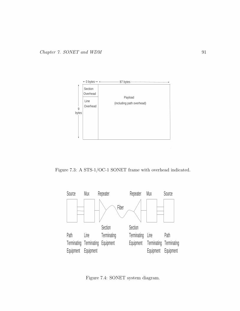
Chapter 7. SONET and WDM 91
Section
Overhead
3 bytes 87 bytes
9bytes
Line
Overhead
Payload
(including path overhead)
Figure 7.3: A STS-1/OC-1 SONET frame with overhead indicated.
PathTerminatingEquipment
LineTerminatingEquipment
PathTerminatingEquipment
LineTerminatingEquipment
SectionTerminatingEquipment
SectionTerminatingEquipment
Fiber
Source Mux SourceMuxRepeater Repeater
Figure 7.4: SONET system diagram.

92 Chapter 7. SONET and WDM
Terminal Node Add/Drop Node Add/Drop Node Terminal Node
Fiber Fiber FiberTM TMADM ADM
TM: Terminal MultiplexerADM: Add/Drop Multiplexer
Figure 7.5: A SONET linear network.
Multiplexer (ADM) in terminal mode. The ADM allows signals to be tapped off or
on the fiber. Alternately, one may have fiber passing through the node. That is, a
fiber enters from the east, for instance, is converted to an electrical signal, signals
are tapped off and inserted and a new fiber leaves to the west. This is called a
SONET ADM in add/drop mode.
7.1.2 Self-Healing Rings
One of the reasons for the widespread use of SONET is it allows a variety of topolo-
gies. The most useful of these are ring topologies. While one can implement linear
add/drop networks (see Figure 7.5), if a fiber in these is cut or an opto-electronic
transceiver fails, one loses complete connectivity.
Typically, rings are implemented with multiple service and protection fibers (see
Figure 7.6). If a service fiber path fails, a protection (back-up) fiber is switched on

Chapter 7. SONET and WDM 93
OC-192
ADM
OC-192ADM
OC-192
ADM
OC-192ADM
servicefiber
protectionfiber
Figure 7.6: A SONET ring network.
its place. The number of protection fibers can be less than the number of service
fibers if one is willing to live with less redundancy. Also, if all of the fibers between
two adjacent nodes are lost, with a sufficient number of protection fiber rerouting
can keep a logical ring in place until repairs are made.
A competitor, at least for data traffic, to SONET is 10 Gbps Ethernet (Meirosu
05).
SONET rates have increased over the years but not by enough for fiber to reach
its full potential unless a second technology, wavelength division multiplexing, is
also used. This WDM technology is discussed in the next section.

94 Chapter 7. SONET and WDM
7.2 Wavelength Division Multiplexing (WDM)
In wavelength division multiplexing (WDM), special multiplexing at either end of a
fiber can put multiple optical signals in parallel on a single fiber (Ryan 98). Thus,
instead of carrying one OC-192 signal at about 10 Gbps, a single fiber might carry
40 OC-192 signals or 400 Gbps of traffic. Even terabit range (1000 Gbps) capacity
is possible. Current systems can have up to about 160 channels. With each signal at
a different optical frequency, WDM is essentially a frequency division multiplexing
scheme.
The history of WDM goes back to a fiber glut in the US that existed prior to
1995. After the Bell System divestiture in the 1980s, the competitors in long distance
phone service had financial limitations so relatively low numbers of fiber per path
were laid (usually about 16 fibers). But by the end of 1995, the interexchange fibers
of the long distance carriers were nearing exhaust. In 1996, 60% of the AT&T
network, 84% of the MCI network and 83% of the Sprint network were fully lit
(Ryan 98).
About this time WDM technology became practical. This technology included
distributed feedback lasers needed to produce the monochromatic output of WDM,
filters to separate signals which are closely packed in frequency and optical amplifiers.
In particular, Erbium Dopel Fiber Amplifiers (EDFA) allowed the amplification of
optical signals without intermediate electronic conversion.
In 1994, Pirelli/Nortel introduced 4 channel systems and IBM introduced a 20
channel system. Cienna followed with a 16 channel system in 1996. By 97/98, 32
and 40 channel systems were being produced. It should be noted that Cienna’s
successful WDM products led to a very successful public offering and 196 million
dollars in first year revenue (the fastest in corporate history at that point).
Now, using WDM in conjunction with SONET, if one had 32 OC-48 channels,
rather than using 32 separate fibers, one could use a 32λ system (32λ means 32

Chapter 7. SONET and WDM 95
wavelengths) on a single fiber or 8 fibers each with OC-192.
Depending on the wavelength assignment WDM systems may be either conven-
tional/coarse (CWDM) or dense (DWDM). More channels are accommodated with
denser channel spacing with DWDM compared to CWDM (Wikipedia).
At first, WDM technology was used in long distance networks but as its costs
decreased, metropolitan area network usage followed.
Tunable lasers have been introduced as a way of providing back-up. That is,
rather than having 176 fixed wavelength spares for a 176λ system, one tunable laser
provides protection against the most likely case, a single bad fixed wavelength laser.
Three generic switching technologies can be used to carry IP traffic over WDM
(Chandra 09). These are optical circuit switching, packet switching and optical
burst switching.
For optical circuit switching to be efficient, like circuit switching in general, the
length of transmissions needs to be significantly greater than the circuit setup time.
This is often not true of bursty data traffic. It has also been shown that the circuit
establishment problem is in general NP hard. That is finding an optimal solution
is computationally intractable though sub-optimal heuristic solution techniques can
be used.
The technology for buffering and packet processing, used by packet switching
techniques, is not yet mature in the optical area making practical, cost efficient,
systems not possible at this time.
The proponents of optical burst switching feels it has the advantages of both
circuit and packet switching. The burst is the fundamental element of optical burst
switching. It can be thought of as a variable length packet with a control header and
the payload to be carried. An optical burst switching system operates over edge and
core routers. Edge (of the network) routers can be either ingress or egress routers.
A variable length burst is assembled at an ingress router from multiple IP packets,

96 Chapter 7. SONET and WDM
possibly from multiple hosts. The burst is transported over the core network and
its routers. At an egress router the burst is disassembled.

Chapter 8
Grid and Cloud Computing
8.1 Introduction
How does cloud computing differ from grid computing? Grid computing usually in-
volves scheduled scientific or engineering computing done on a distributed network of
computers and/or supercomputers. The applications for clouds are often a bit more
mundane but also are more encompassing than grids. The basic idea is that orga-
nizations can rent time on an outside provider’s data center(s) to host applications,
software and services that are more traditionally provided by in house computing
facilities. Both grids and cloud computing are accessed through the Internet.
8.2 Grids
A grid is a distributed computing system that allows users to access large amounts
of computer power and data storage over a network to run substantial computing
tasks. Ian Foster, a leader in grid development, has written (Garritano) that a grid
must
97

98 Chapter 8. Grids and Clouds
• Provide resource coordination without a central control.
• Use standardized and open protocols and interfaces.
• Provide substantial amounts of service involving multiple resource types and
non-trivial user needs.
As Schopf points out, the idea of applying multiple distributed resources to work
on a computational problem is an old one. It goes back at least to the mid six-
ties and the “computer utility” paradigm of the MULTICS operating system and
work on networked operating systems. Further work on distributed operating sys-
tems, heterogeneous computing, parallel distributed computing and metacomputing
further explored this area.
Work on the grid concept started in the mid 1990’s. Among significant grid
features that make it a distinctive problem area are:
• Grids allow site autonomy. Local sites have control over their own resources.
• Grids allow heterogeneity. Grid development work provides standardized in-
terfaces to overcome site diversity.
• Grids are about data (representation, replication, storage in addition to the
usual network and computer issues).
• The key person for grids is the user, not the resource owner. Earlier systems
sought to boost utilization/throughput for the resource owner. In a grid, machines
are selected to fulfill the user’s requirements.
A great deal of grid work is related to interfaces and software development to
allow different sites to work in concert. However, the grid effort has taken time,
enough time that some have questioned its practicality. A balanced discussion of the
difficulties and challenges facing grid development appears in Schopf and Nitzberg.
Here we mention some of these problems.

Chapter 8. Grids and Clouds 99
• In many cases, grids are being used to solve embarrassingly parallel applications
rather than for coordinated distributed computing.
• Users often have to go through a great deal of work to achieve even basic
functionality.
• Some science users see making applications suitable for the grid as a “distrac-
tion” from getting the science accomplished.
• Funding for adapting applications to a grid environment can be drained, if not
blocked, by installation and administration problems.
• System administrators are used to having control over their local resources so
grid software can be seen as “threatening.”
• Setting up an account in a distributed grid can be complex.
An additional problem is that the number of users has not met the expectations
of those who are in favor of grid technology (Schwiegelshohn 10).
However the vision of successful grids may make overcoming these difficulties and
growing pains worthwhile. Quite a few countries have invested in grid infrastructure
to date. Efforts include (Schwiegelshohn 10) D-Grid in Germany (www.d-grid.de),
Grid’5000 in France, DAS in the Netherlands, PL-Grid in Poland (www.plgrid.pl),
NAREGI in Japan (www.naregi.org), and Open Science Grid (www.opensciencegrid.org)
and TeraGrid (www.teragrid.org) in the United States. There are some grids for
communities using large amounts of data such as for particle physics.
The Open Grid Service Architecture is an important grid standard announced
in 2002. The service oriented architecture of OGSA is illustrated in Fig. 1.1.
In the figure, note that OGSA services are presented to the application layer.
Also, OGSA services make use of web services. Note also this grid architecture has
three hardware components: servers, storage and networks. A document discussing
the architecture of OGSA can be found on Wikipedia.

100 Chapter 8. Grids and Clouds
Messaging
Applications
OGSA Services
Web Services
Security Workflow Database File Systems Directory
Servers Storage Networks
Figure 8.1: Open Grid Service (OGSA) Architecture.
The main grid standards setting body is the Open Grid Forum. It was created
from the merger of the Global Grid Forum and the Enterprise Grid Alliance in
2006. The Open Grid Forum is responsible for standards such as OGSA, Open Grid
Services Infrastructure (OGSI), Job Submission Description Language (JSDL) and
GridFTP. It has also done recent work on cloud computing. Other organizations
who have had grid involvement include the Organization for the Advancement of
Structured Information Standards (OASIS), the World Wide Web Consortium, the
Distributed Management Task Force, the Web Services Inter-operability Organiza-
tion and some groups in Internet 2 such as the Peer-to-Peer Working Group, the
Middleware Architecture Committee for Education and the Liberty Alliance (Baker
05).
For further information readers are referred to Schwiegelshohn 10, www.gridforum.org
and www.globus.org.

Chapter 8. Grids and Clouds 101
8.3 Cloud Computing
Again, under the usual cloud computing paradigm an organization can rent time on
a provider’s data center(s) resources to host applications, software and services that
to date have been provided on in house computing facilities. There are three main
types of cloud computing services (Sultan 10, Zissis 11):
Software as a Service (Saas): This allows a user (a consumer, student, employee
of a business) to use applications accessed through the Internet that are run on the
facilities of the entity supplying the service at a data center “inside the cloud.” Thus
the user only needs a web browser, not the actual application software. The user
does not directly manage the cloud infrastructure (servers, storage etc..).
Infrastructure as a Service (Iaas): Provides a complete computer infrastructure
over the Internet (virtual computers, services, storage etc..).
Platform as a Service (Paas): User essentially has a “virtual platform” accessed
through the Internet. The user can load applications using languages and/or tools
that are supported by the cloud service provider. Users control applications but not
the supporting infrastructure.
Zissis and Lekkas (Zissis 11) describe four ways in which clouds can be used:
• Private Cloud: A private entity/organization uses cloud facilities dedicated for
its own use. These facilities may be administered by the organization itself or a
different entity and may be on site or off site.
• Community Cloud: The cloud facilities are shared by a community of several
related entities. Again, it may be operated by the entities or a different entity and
may be on site or off site.
• Public Cloud: Cloud facilities owned by an entity selling cloud services are
offered to the general public, industry, government or a selected group of such.

102 Chapter 8. Grids and Clouds
• Hybrid Cloud: An aggregation of at least two clouds of the previous types that
support application and/or data portability for load balancing among the clouds.
8.3.1 Tradeoffs for Cloud Computing
Like any relatively new technology, cloud computing has a number of advantages
and disadvantages (Marston 11, Zissis 11). Among the advantages are:
• Cost: By “renting” services an organization can avoid large capital invest-
ments in infrastructure. Cloud service providers can take advantage of economies of
scale through locating data centers on inexpensive real estate and in areas with low
power costs and by aggregating the stochastic demand of a number of users into a
centralized, expertly managed facility.
• Flexibility: Users can quickly have access to computing resources. Provisioning
is elastic and fast. Services can be scaled according to client demand.
• New Services: New, innovative applications can be deployed in a straightfor-
ward manner. Such applications include parallel batch processing, business analytics
and social media such as FaceBook and YouTube.
What of disadvantages? A major issue for organizations thinking about cloud
computing is the loss of direct control of their data. Is the entity providing cloud
computing services trustworthy? Do they run secure facilities? Are they liable to
go out of business suddenly causing a loss of data?
As a niche example, the University of Westminster in the UK transitioned to a
Google based email system. However they continued to maintain records, intellectual
property, legal, research and employment information on university owned systems
(Sultan 10).
Related to this is the issue of cloud security. This includes protection of data
and integrity of applications. Some feel (Pacella 11) that we are in a nascent era of

Chapter 8. Grids and Clouds 103
cloud attacks by hackers. Cloud computing is built on easy access unlike systems
that are protected behind a firewall. Hijacked cloud computing infrastructure could
be used for distributed denial of service attacks. Hijacked resources in a cloud could
be used for a cross-cloud attacks on cloud users.

104 Chapter 8. Grids and Clouds

Chapter 9
Data Centers
9.1 Introduction
Data centers are networked collections of computers that provide the computational
resources for web-hosting, e-commerce, grid and cloud computing and social net-
working in a centralized location. Generic service platforms for this purpose include
Sun’s Grid Engine, Google’s App engine, Amazon’s EC2 platform and Microsoft’s
Azure platform. In the following we largely follow the excellent treatment in (Kant
09).
Virtualization, the ability of a data center to service many independent users
while giving each user the impression of a dedicated facility, is important in data
center technology for providing good server utilization and for making resource al-
location flexible. Because of virtualization, data center management is not a simple
problem. The expected trend in data center development is that data centers will
become more virtualized, distributed and a “multi-layer infractructure” (Kant 09).
This will lead to a number of difficult technological problems.
105

106 Chapter 9. Data Centers
9.2 Data Centers
9.2.1 Racks
The personal computer-like computers (servers) used in data centers are mounted
in racks. A rack will actually contain not only the servers but often storage and
specialized devices. A standard rack is 78 inches high, 23 to 25 inches wide and 26 to
30 inches deep. Assets mounted in a rack are measured in “U”’s (i.e 45 mm or about
1.8 inches). A single or dual processor may be 1U. A four socket multiprocessor may
be 2U or more. A standard rack can accommodate 42 1U assets (Kant 09).
Servers can be in a 13 inch high chassis. Six of these can be inserted into a rack
since 6 times 13 is 78 inches (typical chassis height). A chassis will have a power
supply, a backplane interconnect, fans and management support. Sixteen 1U servers
can be placed in a chassis so that a rack can hold 6 times 16 or 96 servers. “Blades”
are modular assets in a chasis.
Racks vary greatly in their complexity. They may or may not include a metal
enclosure, rack power distribution, air or liquid cooling at the rack level, a keyboard,
video monitor and mouse (e.g. kvm switch) and rack level management unit.
Power is a key consideration in data center design and operation. Kant reports
that racks in older data centers may utilize 7 kW per rack and a loaded blade server
rack may utilize 21 kW.
9.2.2 Networking Support
Data centers often are equipped with Infiniband, Ethernet, lightweight transport
protocols implemented over Ethernet and/or PCI-Express based backplane intercon-
nect. Wireless networking tends to be a niche technology in data centers. Another
issue is that with increasing transmission speeds, protocols need to be lightweight

Chapter 9. Data Centers 107
(i.e. simple). However there is a need for some complexity because of security and
other needed functionality.
There are at least four types of network access for a data center. This can lead
to the use of several (even four) networking technologies in a data center (Kant 09).
(1) Client-server network for data center access: This could utilize Ethernet or
wireless LAN technology.
(2) Server-server network: This operates at high speed and may utilize Ethernet,
Infiniband or other networking technologies.
(3) Access to storage: Historically this may use Fibre channel technology but
storage access can also use technologies such as Ethernet or Infiniband.
(4) Management network: could be Ethernet or a side channel on the main
network.
Often the uplinks are “over-subscribed.” One speaks of an over-subscription ra-
tio as it may not be possible to achieve the full bisection bandwidth. Bisection
bandwidth is the worst case bandwidth between a segmentation of a network into
two equal parts. For instance if 15 servers at 1Gbps each share a 10 GBps link, the
over-subscription ratio is 1.5.
Tree networks, traditionally used in data centers, have a problem in that they
can have less cross section bandwidth than would be ideal. Fat trees and other types
of interconnection networks have been suggested to alleviate this problem.
Mitigating or preventing denial of service attacks is another concern for data
centers (Kant 09).

108 Chapter 9. Data Centers
9.2.3 Storage
Storage capacity and data generation volume continues to increase at a great rate
(some estimates are 50 to 70% growth a year).
Storage usually has used rotating magnetic technology to date. Because of rotat-
ing discs’s mechanical construction sequential access is faster than random access.
Storage can be responsible for twenty to thirty percent of a data center’s power usage.
A relatively new technology is solid state storage (non-volatile RAM or NVRAM).
Kant (Kant 09) suggests that solid state storage will be in a “supporting” role for
rotating discs for the near future.
In data centers one has (Kant 09):
· DAS (Direct Access Storage): direct connection to server.
· SAN (Storage Area Network): storage (block oriented) exists across the net-
work.
· NAS (Network Attached Storage): storage (files or objects) exists across the
network.
Data intensive applications, streaming and search create large loads on the stor-
age system. It tends to be less expensive to carry all types of networking load on
Ethernet but basic Ethernet does not have quality of service (QoS) support.
9.2.4 Electrical and Cooling Support
A medium sized data center can require several meagwatts in peak power. Power is
provided to the data center on high voltage lines such three phase 33 kvolts lines.
Transformers on premises step it down to three phase power at 280 to 480 volts.
Power then goes to uninterruptible power supplies (UPS). The UPS output is often
single phase power at 120 to 240 volts. This is supplied to a power distribution unit

Chapter 9. Data Centers 109
which provides electric power to a rack mounted chassis or blade chassis. Power
here is stepped down and converted to DC from AC to provide plus or minus 5 volts
or plus and minus 12 volts. Voltage regulators on the mother board change this to
even lower voltages for the rails such as 1.1 volts, 5 volts and 12 volts.
With power conversion efficiencies of 85% to 95% at each step (and 50% or so at
the mother board rails) there is a great deal of energy loss and room for improvement.
Data center power usage as a percentage of US power consumption doubled from
2000 to 2007 and is expected to double again by 2012 (Kant 09).
Cooling can account for 25% or so of a data center’s electric power usage. Air
may enter racks at 21 degree centigrade and leave at 40 degree centigrade. Cooling
necessitates building air conditioning units as well as large chiller plants, air re-
circulation systems and fans.
Improving power usage can be done in a number of ways (Kant 09):
· Designing hardware and software for low power consumption.
· Designing the occurrence of hardware power states to minimize power con-
sumption. This includes for CPU’s, interconnection networks and for memory. An
example might be a low power sleep state for a piece of hardware when not being
actively used.
· In general, power appropriate use and regulation of data center infrastructure.
One metric for measuring the efficiency of a data center is power-usage effec-
tiveness (PUE) (Schneider 11). This is the ratio of the total power used by a data
center to the power consumed by just the computers and and networking equipment.
Schneider and Hardy report that Google achieved an “overall” PUE of 1.13 at the
end of 2010 and Facebook “believes” its new data centers will have a PUE value of
1.07 or lower.
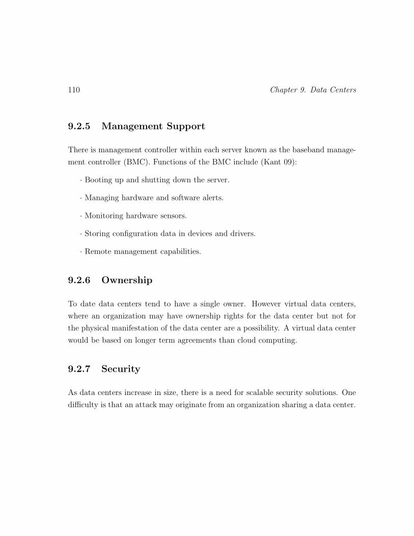
110 Chapter 9. Data Centers
9.2.5 Management Support
There is management controller within each server known as the baseband manage-
ment controller (BMC). Functions of the BMC include (Kant 09):
· Booting up and shutting down the server.
· Managing hardware and software alerts.
· Monitoring hardware sensors.
· Storing configuration data in devices and drivers.
· Remote management capabilities.
9.2.6 Ownership
To date data centers tend to have a single owner. However virtual data centers,
where an organization may have ownership rights for the data center but not for
the physical manifestation of the data center are a possibility. A virtual data center
would be based on longer term agreements than cloud computing.
9.2.7 Security
As data centers increase in size, there is a need for scalable security solutions. One
difficulty is that an attack may originate from an organization sharing a data center.

Chapter 10
Advanced Encryption Standard(AES)
10.1 Introduction
The Advanced Encryption Standard (AES) is the encryption standard approved in
2000 under the auspices of the US government, originally for civilian cryptographic
use. In 2003 the United States government approved the use of AES for classified
and secret information. Versions of AES for 192 bit and 256 bit keys are approved
for top secret information. The National Institute of Standards and Technology,
which led the three year approval process for AES, has certified in excess of 1000
products incorporating AES (Daemen 10). The Advanced Encryption Standard is
incorporated in standards, algorithms and requests for comments from IEEE (In-
stitute of Electrical and Electronics Engineers), IETF (Internet Engineering Task
Force), ISO (International Organization for Standardization)and 3GPP (Third Gen-
eration Partnership Project, see wireless chapter). The use of AES in hardware and
smart cards is taking longer but progress is being made.
111

112 Chapter 10. AES
10.2 DES
The predecessor to AES was DES (Digital Encryption Standard). The National
Bureau of Standards, which eventually became NIST, called for proposals for a
block encryption standard (i.e. encrypting a block of data at a time rather than a
continuous stream of data as a stream cipher would) in 1973 (Burr 03). The only
practical candidate was one from IBM. This was modified into what became known
as DES.
There were some public issues concerning DES. The original 128 bit key was re-
duced to 56 bits in DES. Some changes were also made to scrambling boxes known as
“S boxes”. Some felt that without knowing the reasons for the DES modifications it
was difficult to make an assessment of its security. When differential cryptanalysis1
was discovered some time later it was found that DES was more resistant to differ-
ential cryptanalysis because of the S box changes. It was conjectured that IBM and
NSA (the US code breaking and creation agency) knew of differential cryptanalysis
and the changes were made for this reason (Burr 03).
As Burr (Burr 03) puts it, DES is the standard against which all block ciphers
are compared.
In 2004 NIST withdrew DES through a version using three keys/steps of encryp-
tion and decryption, triple DES, is still approved.
10.3 Choosing AES
It is interesting to briefly discuss the selection process that led to the choice of the
current AES (the summary here is largely based on the excellent discussion in Burr
03).
1A technique where small changes to input are correlated with output changes to attempt tofind the key.

Chapter 10. AES 113
At the time of the selection of DES, the thought was that encryption is best
done in hardware. But DES is not well suited for software operation. One needs to
shuffle/scramble 4 or 6 bits. This fast in hardware but slow on computers. Moreover
triple DES is three times slower than DES. As the years went by, software encryption
became more important.
NIST created a selection process for AES for federal and international business
purposes. Among the properties an acceptable AES would need are (Burr 03):
• Should be a block cipher.
• It should be at least as secure as triple DES.
• 128 bit block size.
• options for key sizes of 128, 192 and 256 bits.
• It should be unclassified and open to the public (not patented and royalty
free).
Fifteen qualifying groups submitted proposals in 1998. The next year there were
five final candidates:
• MARS from IBM (US).
• RC6 from RSA Data Systems (US).
• Rijndael from Joan Daemen and Vincent Rijmen (Belgium).
• Serpent from Ross Anderson, Eli Biham and Lars Knudsen (UK, Israel and
Denmark).
• Twofish from a team of American companies and academics (US).
Burr’s 2003 article describes each contender.
In 2000 NIST selected Rijndael as the new AES. Rijndael was the most popular

114 Chapter 10. AES
finalist in polls at the most recent AES conference. The international cryptographic
community was well disposed towards it. Finally, the selection of a non-US cipher
made international acceptance smoother. Rijndael was made the official AES in
Dec. 2001.
10.4 AES Issues
NIST’s criteria for selecting AES included security, performance and intellectual
property.
10.4.1 Security Aspect
It was thought about 2003 (Burr 03) that an 80 bit key would provide sufficient
protection against exhaustive search for a limited number of years. Moreover if
Moore’s law (computing power doubling every 18-24 months) remains true a 128 bit
key would provide protection until 2066 and a 256 bit key would provide protection
for several centuries. Of course what form technology will take centuries from now
is hard to predict and breakthroughs like practical and robust quantum computing
may change the situation radically.
Most symmetric key algorithms consist of multiple iterations/repetitions of a
(scrambling) function called a round function (Burr 03). People evaluating codes
will try to find short cuts on simpler versions of an encryption algorithm that use less
than the full set of rounds. The attack will then be tried on the complete algorithm.
People creating encryption algorithms estimate the number of rounds needed for
security and add to this additional rounds as a safety margin.
An encryption algorithm is deemed secure if no short cuts are known. The longer
it has been evaluated the more confidence one has in its security. But encryption
products are different from typical products. With a typical product it is designed,

Chapter 10. AES 115
tested and fielded. While surprises are certainly possible after it is fielded, they are
rare. With an encryption algorithm no matter how much effort goes into its design,
one is never quite sure in the back of one’s mind if there is some clever way to crack
it.
For the full versions of the final contenders in the AES competition no shortcuts
were found. Attacks were found for versions of the final contenders with fewer
rounds. Actually it wasn’t possible to differentiate between the contenders on the
basis of security. As reported by Burr (Burr 03) the best attack against Rijndael
worked on 7 of 10 rounds and needed 2127 pairs, 2101 bytes of memory and 2120
operations. Subsequent attacks aimed at breaking AES have only been successful
on reduced versions of AES (Daemen 10).
There are arguments about whether a simple or a complex encryption algorithm
provides better security. A simpler algorithm can be better understood but some feel
because it is simple a new attack may crack (break) it. For a complex algorithm if
one part is broken the other parts may still provide backup security, some hold. But a
complex algorithm may be difficult to fully analyze so there may be an unknown way
an attacker may succeed in breaking it. The creators of Rijndael believe simplicity
is the better virtue (Daemen 10).
10.4.2 Performance Aspect
The performance of the candidate algorithms in the AES selection process were first
discussed for 32 bit Pentiums. There was at least moderate performance for all of
the contenders on Pentiums. All of the contenders had a better performance than
triple DES. Performance was also examined based on RISC processors, Itaniums, 8
bit embedded microprocessors, digital signal processors (DSP), field programmable
gate arrays (FPGA) and application specific integrated circuits (ASIC) (Burr 03).
116 Chapter 10. AES
10.4.3 Intellectual Property Aspect
It was desired that AES be available royalty free on world wide basis. This goal was
made easier because DES patents had expired and there were quite a few algorithms
available that were not patented. It was found by NIST that the final contenders’
algorithms did not infringe on any existing patent.
There was also some question as to whether NIST should choose one winner or
more than one. Straw polls at the third AES conference indicated that one winner
was the community’s preference. One reason (Burr 03) is that choosing several
algorithms might lead to compatibility problems, require more chip real estate and
there would be a higher probability of intellectual property issues.
10.4.4 Some Other Aspects
It takes more than encryption algorithms to make secure systems. For instance,
sending an email may require a public key transport algorithm, public key signature
algorithm, a hash algorithm and then the (AES) encryption algorithm (Burr 03).
Work has gone on in standardizing other strong algorithms in addition to encryption
algorithms.
Another issue is that block ciphers such as DES and AES can be used in a
number of well known “modes” of operation. These include:
• Electronic Code Book Mode: A plaintext number of bits is mapped into the
same number of encrypted bits. A weakness is that an attacker may swap sections
of the code with code of their own.
• Cipher Block Chaining Mode: One linearly chains block ciphers so replacing a
block causes unintelligible code after that point.
• Cipher Feedback Mode: Uses feedback in the coding process for byte by byte

Chapter 10. AES 117
encryption.
• Stream Cipher Mode: A simple way to convert any block cipher to a stream
cipher (i.e. encrypting a continuous stream of data rather than a block at a time).
A weakness of chained and feedback modes is that they can’t be parallelized and
they can’t be arbitrarily accessed (one needs to start at the beginning). To address
this a counter mode was introduced which is parallelizable (Burr 03).
Other modes have been proposed to NIST. Some are parallelizable and do en-
cryption, authentication and integrity protection for just a bit more than the cost
of encryption. However the inventors filed patents on these so there are some intel-
lectual property issues.

118 Chapter 10. AES

Chapter 11
Bibliography
119

120 Bibliography

Bibliography
[1] S. Ahmadi, “An Overview of Next-Generation Mobile WiMAX Technol-
ogy,” IEEE Communications Magazine, June 2009, pp. 84-98.
[2] I.F. Akyildiz, D.M. Gutierrez-Estevez and E.C. Reyes, “The Evolution
to 4G Cellular Systems: LTE Advanced,” Physical Communication, 3,
2010, pp. 217-244.
[3] G. Armitage, “MPLS: The Magic Behind the Myths,” IEEE Communi-
cations Magazine, Jan. 2000, pp. 124-131.
[4] A. Bacioccola, C. Cicconetti, C. Eklund, L. Lenzini, Z. Li and E. Min-
gozzi, “IEEE 802.16: History, Status and Future Trends,” Computer
Communications, vol. 33, 2010, pp. 113-123.
[5] M. Baker, A. Apon, C. Feiner and J. Brown, “Emerging Grid Standards,”
Computer, vol. 38, no. 4, 2005, pp. 43-50.
[6] O. Banimelhem, J.W. Atwood and A. Agarwal, “Resiliency Issues Issues
in MPLS Networks,” Canadian Conference on Electrical and Computer
Engineering, CCGEI 2003, Montreal, Quebec, May 2003, pp. 1039-1042.
[7] W.E. Burr, “Selecting the Advanced Encryption Standard,” IEEE Secu-
rity and Privacy, March/April 2003, pp. 43-52.
121

122 Bibliography
[8] P.K. Chandra, A,K. Turuk nd B. Sahoo, “Survey on Optical Burst
Switching in WDM Networks,” Proceedings of the Fourth International
Conference on Industrial and Information Systems, ICIIS 2009, 2009,
pp. 83-88.
[9] J.M. Chung, H.K. Khan, H.M. Soo, J.S. Reyes and G.Y. Cho, “Analysis
of GMPLS Architectures, Topologies and Algorithms,” Proceedings of the
2002 45th Midwestern Symposium on Circuits and Systems MWSCAS-
2002, vol. 3, 2002, pp. 284-287.
[10] J. Daemen and V. Rijmen, “The First 10 Years of Advanced Encryption,”
IEEE Security and Privacy, Nov/Dec 2010, pp. 72-74.
[11] J. D’Ambrosia, D. Law and M. Nowell, “40 Gigabit Ethernet
and 100 Gigabit Ethernet Technology Overview,” Ethernet Alliance,
www.ethernetalliance.org, 2008.
[12] J.P. Dunning, “Taming the Blue Beast: A Survey of Bluetooth-Based
Threats,” IEEE Security and Privacy, March/April 2010, pp. 20-27.
[13] C. Eklund, R.B. Marks, K.L. Stanwood and S. Wang, “IEEE Standard
802.16: A Technical Overview of the Wireless MAN Interface for Broad-
band Wireless Access,” IEEE Communications Magazine, June 2002, pp.
98-107.
[14] T. Garritano, “Globus: An Infrastructure for Resource Sharing,” Clus-
terworld, vol. 1, no. 1, pp. 30-31, 50.
[15] R.C. Garroppo, S. Giordano and L. Tavanti, “Implementation Frame-
works for IEEE 802.11s Systems,” Computer Communications, vol. 33,
2010, pp. 336-349.
[16] L. Goldberg, “802.16 Wireless LANs: A Blueprint for the Future?,” Elec-
tronic Design, Aug. 4, 1997, pp. 44-52.

Bibliography 123
[17] P. Grun, “Introduction to Infiniband for End Users,” Infiniband Trade
Association, www.infinibandta.org, 2010.
[18] J.C. Haartsen and S. Mattisson, “Bluetooth - A New Low-Power Radio
Interface Providing Short-Range Connectivity,” Proceedings of the IEEE,
vol. 88, no. 10, Oct. 2000, pp. 1651-1661.
[19] G.R. Hiertz, D. Denteneer, S. Max, et. al., “IEEE 802.11s: The WLAN
Mesh Standard,” IEEE Wireless Communications, Feb. 2010, pp. 104-
111.
[20] J.M. Kahn, R.H. Katz, K.S.J. Pister, “Emerging Challenges: Mobile
Networking for “Smart Dust”,” Journal of Communication Networks, vol.
2, no. 3, Sept. 2000.
[21] K. Kant, “Data Center Evolution: A Tutorial on State on the Art, Issues
and Challenges,” Computer Networks, vol. 53, 2009, pp. 2939-2965.
[22] S. Kapp, “802.11: Leaving the Wire Behind,” IEEE Internet Computing,
vol. 6, no. 1, Jan-Feb 2002, pp. 82-85.
[23] M.S. Kuran and Y. Tugcu, “A Survey on Emerging Broadband Wireless
Access Technologies,” Computer Networks, vol. 51, 2007, pp. 3013-3046.
[24] K.S. Kwak, S. Ullah and N. Ullah, “An Overview of IEEE 802.15.6 Stan-
dard,” 3rd International Symposium on Applied Sciences in Biomedical
and Communication Technologies (ISABEL), 2010, pp. 1-6.
[25] R.O. LaMaire, A. Krishnan, P. Bhagwat and J. Panian, “Wireless LANs
and Mobile Networking Standards and Future Directions,” IEEE Com-
munications Magazine, vol. 34, no. 8, Aug. 1996, pp. 86-94.
[26] B. Latre, B. Braem, I. Moerman, C. Blondia, P. Demeester, “A Survey
on Wireless Body Area Networks,” Wireless Networks vol. 17, 2011, pp.
1-18.

124 Bibliography
[27] J. Lawrence, “Designing Multiprotocol Label Switching Networks,” IEEE
Communications Magazine, July 2001, pp. 134-142.
[28] A. Leon-Garcia and L.G. Mason, “Virtual Network Resource Manage-
ment for Next-Generation Networks,” IEEE Communications Magazine,
July 2003, pp. 102-109.
[29] T. Li, “MPLS and the Evolving Internet Architecture,” IEEE Commu-
nications Magazine, Dec. 1999, pp. 38-41.
[30] E. van der Linde and G.P. Hancke, “An Investigation of Bluetooth Mer-
gence with Ultra Wideband,” Ad Hoc Networks, vol. 9, no. 5, 2011, pp.
852-863.
[31] M. Littlewood and I.D. Gallagher, “Evolution Toward an ATD Multi-
service Network,” British Telecom Technology Journal, vol. 5, no. 2, April
1987.
[32] S. Marston, Z. Li, S. Bandyopadhyay, J. Zhang and A. Ghalsasi, “Cloud
Computing - The Business Perspective,” Decision Support Systems, vol.
51, 2011, pp. 176-189.
[33] J.L. Marzo, E. Calle, C. Scoglio and T. Anjali, “QoS Online Routing and
MPLS Multilevel Protection: A Survey,” IEEE Communications Maga-
zine, Oct. 2003, pp. 126-132.
[34] M. Mauve, H. Hastenstein and A. Widmer, “A Survey of Position-Based
Routing in Mobile Ad Hoc Networks,” IEEE Network, vol. 15, no. 3,
Nov/Dec 2001, pp. 30-39.
[35] C. Meirosu, P. Golonka, A. Hirstius, et. al., “Native 10 Gigabit Eth-
ernet Experiments over Long Distances,” Future Generation Computer
Systems, vol. 21, 2005, pp. 457-468.

Bibliography 125
[36] C. Metz, C. Barth and C. Filsfils, “Beyond MPLS...Less is More,” IEEE
Internet Computing, Sept./Oct. 2007, pp. 72-76.
[37] J. Moy, “OSPF Version 2,” RFC 2178, April 1998.
[38] C.S.R. Murthy and B.S. Manoj, Ad Hoc Wireless Networks: Architectures
and Protocols, Prentice-Hall, Upper Saddle River NJ, 2004.
[39] M. Nowell, V. Vusirikala and R. Hays, “Overview of Requirements and
Applications for 40 Gigabit and 100 Gigabit Ethernet,” Ethernet Alliance,
version 1.0, www.ethernetalliance.org, 2007.
[40] R.O. Onvural, Asynchronous Transfer Mode Networks: Performance Is-
sues, Artech House, 2nd edition, 1995.
[41] R.M. Pacella, “Hacking the Cloud,” Popular Science, April 2011, pp.
68-72.
[42] D. Papadimitriou and D. Verchere, “GMPLS User-Network Interface in
Support of End-to-End Rerouting,” IEEE Communications Magazine,
July 2005, pp. 35-43.
[43] I. Papapanagiotou, D. Toumpakaris, J. Lee and M. Devetsikiotis, “A Sur-
vey on Next Generation Mobile WiMAX Networks: Objectives, Features
and Technical Challenges,” IEEE Communications Surveys and Tutori-
als, vol. 11, no. 4, 2009, pp. 3-18.
[44] C.E. Perkins, Ad Hoc Networks, Addison-Wesley, Boston, Massachusetts,
2001.
[45] S.W. Peters and R.W. Heath, Jr., “The Future of WiMAX: Multihop Re-
laying with IEEE 802.16j,” IEEE Communications Magazine, Jan. 2009,
pp. 104-111.

126 Bibliography
[46] I. Poole, “What Exactly is 802.11n?,” Communication Engineer, Febru-
ary/March, 2007, pp. 46-47.
[47] I. Poole, “What Exactly Is... LTE?,” Communications Engineer,
June/July 2007, pp. 46-47.
[48] J.M. Rabaey, M.J. Ammer, J.L. da Silva Jr., et. al., “PicoRadio Supports
Ad Hoc Ultra-Low Power Wireless Networking,” Computer, vol. 33, no.
7, July 2000, pp. 42-48.
[49] M. Rinne and O. Tirkkonen, “LTE, The Radio Technology Path Towards
4G,” Computer Communications, vol. 33, 2010, pp. 1894-1906.
[50] T.G. Robertazzi, Peformance Evaluation of High Speed Switching Fab-
rics and Networks: ATM, Broadband ISDN and MAN Technology, IEEE
Press, 1993 (now distributed by Wiley).
[51] T.G. Robertazzi, Networks and Grids: Technology and Theory, Springer,
New York NY, 2007.
[52] J.P. Ryan, “WDM: North American Deployment Trends,” IEEE Com-
munications Magazine, vol. 36, no. 2, Feb. 1998, pp. 40-44.
[53] D. Schneider and Q. Hardy, “Under the Hood at Google and Facebook,”
IEEE Spectrum, vol. 48, no. 6, June 2011, pp. 63-67.
[54] J.M. Schopf and B. Nitzberg, “Grids: The Top Ten Questions,” Scientific
Programming, IOS Press, vol. 10, no. 2, 2002, pp. 103-111.
[55] M. Schwartz, Telecommunication Networks: Protocols, Modeling and
Analysis, Addison-Wesley, Reading, Mass., 1987.
[56] L. Schwiebert, S.K.S. Gupta and J. Weinmann, “Research Challenges
in Wireless Networks of Biomedical Sensors,” ACM Sigmobile, 2001, pp.
151-165.

Bibliography 127
[57] U. Schwiegelshohn, R.M. Badia, et. al., “Perspectives on Grid Comput-
ing,” Future Generation Computer Systems, vol. 26, 2010, pp. 1104-1115.
[58] R.C. Shah and J.M. Rabaey, “Energy Aware Routing for Low Energy Ad
Hoc Networks,” Proceedings of the 3rd IEEE Wireless, Communications
and Networking Conference, 2002, pp. 350-355.
[59] S. Siwamogsatham, “10 Gbps Ethernet,” 1999, www.cse.wustl.edu/jain
[60] W. Stallings, High-Speed Networks and Internets: Performance and Qual-
ity of Service, Prentice-Hall, 2002.
[61] N. Sultan, “Cloud Computing for Education: A New Dawn,” Interna-
tional Journal of Information Management, vol. 30, 2010, pp. 109-116.
[62] A. Tanenbaum, Computer Networks 3rd ed., Prentice-Hall, 1996.
[63] A. Tanenbaum, Computer Networks, 4th ed., Prentice-Hall, 2003.
[64] M. Tatipamula, F. Le Faucheur, T. Otani and H. Esaki, “Implementa-
tion of IPv6 Services over a GMPLS-Based IP/Optical Network,” IEEE
Communications Magazine, May 2005, pp. 114-122.
[65] S.J. Vaughan-Nichols, “Will 10-Gigabit Ethernet Have a Bright Future?,”
Computer, June 2002, pp. 22-24.
[66] S.J. Vaughan-Nichols, “Will the New Wi-Fi Fly?,” Computer, Oct. 2006.
pp. 16-18.
[67] http://www.wikipedia.org
[68] X. Xiao and L.M. Ni, “Internet QoS: A Big Picture,” IEEE Network,
March/April 1999, pp. 8-18.

128 Bibliography
[69] D. Yang, Y. Xu and M. Gidlund, “Coexistence of IEEE802.15.4 Based
Networks: A Survey,” Proceedings of the 36th Annual IEEE Conference
on Industrial Electronics (IECON 2010), 201. pp. 2107-2113.
[70] J. Zheng and M.J. Lee, “Will 802.15.4 Make Ubiquitous Networking a Re-
ality? A Discussion on a Potential Low Power, Low Bit Rate Standard,”
IEEE Communications Magazine, June 2004, pp. 140-146.
[71] D. Zissis and D. Lekkas, “Addressing Cloud Computing Security Issues,”
Future Generation Computer Systems, article in press as of April 2011.

Chapter 12
Index
129

Index
3GPP, 64
802.3, 23-28
802.4, 23
802.5, 23
802.11, 45-50
802.15, 51-57
802.16, 58-63
Ad hoc network, 9-10
AES, 111-117
AMPS, 9
Application layer, 19
ATM, 69-78
Binary exponential backoff, 25
Bluetooth, 51-57
Cable TV, 2-3
Cellular system, 8-9
Circuit switching, 16-18
Cloud computing, 101-103
Coaxial cable, 2-3
CSMA/CA, 47
CSMA/CD, 25
Data centers, 105-110
Data link layer, 20
DES, 112
Direct Sequence Spread Spectrum, 14-16
Ethernet
10 Mbps, 24-28
100 Mbps, 28-30
1 Gbps, 30-31
10 Gbps, 32-34
40 Gbps, 35-37
100 Gbps, 35-37
Femtocells, 67
Fiber optics, 4-5
Frequency division multiplexing, 12-13
Frequency hopping, 14
Geostationary orbit, 5-6
GMPLS, 85
Grids, 97-100,
GSM, 9
Hub 24, 28
InfiniBand, 39-44
Iridium, 6-8
130

Index 131
ISM band, 46
Layered protocols, 18-21
LEOS, 6-8
Line layer, 90
LTE, 64-66
LTE Advanced, 66-67
Manchester encoding, 26
Microwave LOS, 5
Modulation, 2
MPLS, 79-85
Multimode fiber, 4
Multiplexing, 12-16
Network layer, 20
NNI, 71-74
Packet switching, 16-18
Path layer, 90
Physical layer, 21
Picocell, 67
Position based routing, 10-11
Presentation layer, 20
QAM, 56
QPSX, 56
Racks, 106
RDMA, 39-40
Rijndael, 113-114
RM cells, 74-75
Satellites, 5-8
Self-healing rings, 92-93
Session layer, 20
Shared medium switch, 76
Shared memory switch, 77-78
Single mode fiber, 4
SONET, 87-93
Space division switching, 78
STM, 70-71
STS/OC (SONET) rates, 88
Time division multiplexing, 13-14
Topology based routing, 10
Traffic engineering, 83-84
Transport layer, 20
Twisted pair wiring, 3-4
UNI, 71-74
UNI bands, 49
Virtual circuits, 17
Virtual tributary, 88
Virtualization, 105
WBAN, 56-57
WDM, 94-96
WiFi, 45-51
WiMax, 58-62
Wireless sensor network, 11-12
Zigbee, 54-56