basics of local optimization - university of cambridgempj1001/papers/anade_local...basics of local...
TRANSCRIPT

Basics of Local Optimization
J. Peter, M. Bompard - ONERA The French Aerospace Lab.
ANADE Workshop – Cambridge september 24th 2014

Basics of Local Optimization ANADE Workshop 24/09/14
OPTIMIZATION
Mathematics and Mechanics
• Slides from those a RTO lecture series
• RTO-AVT-167 group Strategies for Optimization and Automated Design of Gas Turbine Engines
2008-2010
• Lecture notes available on S&T web site Local Search Methods for Design in Aeronautics
M. Bompard, J. Peter (46 pages) More details than in these slides
Basics of Local Optimization ANADE Workshop 24/09/14
OPTIMIZATION
Mathematics and Mechanics
• Classical optimization problems in Mechanics
. Minimize the drag of an aircraft under constraints (on lift, pitching mo-
ment...). Maximize total pressure of supersonic aircraft air intake
. Maximize efficiency of a turbomachinery blade under constraints (on surge
margin - compressor / on aerothermal behaviour - turbine)
• General mathematical counterpart
. All possible shapes = infinite dimensional search
. Partial differential equations, unsolvable for complex shapes and B.C.
• Need for simplification - discretization and parametrization
Basics of Local Optimization ANADE Workshop 24/09/14
OPTIMIZATION
Mathematics in finite dimension and Mechanics
• Classical optimization problems in Mechanics
• Using numerical analysis and parametrization
. Mesh (some hundreds of thousands/milions points) - baseline shape
. Numerical analysis (finite volumes for (RANS) equations...)
. Design parameters describing the possible deformed shapes
• Solvable, finite dimensional mathematics
• Optimization with large design space and complex direct problem very expensive
. Sampling of all design space plus computation of all points : unaffordable
. Efficient optimization algorithms required
Basics of Local Optimization ANADE Workshop 24/09/14
OPTIMIZATION
Local and global optimization - Mathematics (1/3)
• Definitions and notations
. α vector of parameters
. Dα design space = Region of Rnf associated to the parametrization
. Mechanics - objective : function that has to be maximized/minimized
→ Maths - function J (α) to minimize
. Mechanics - constraints : functions that have to be kept lower/higher than
some value→ Maths - functions Gk(α) that should verify Gk(α) ≤ 0.
• With or without equality constraints ?
. Each time it is possible
→ Change parametrization
→ Define a design space of smaller dimension in the subspace
defined by former equality constraint. No equality constraint considered in this course
Basics of Local Optimization ANADE Workshop 24/09/14
OPTIMIZATION
Local and global optimization - Mathematics (2/3)
• Global optimization
. Goal = find the best solution/shape α∗ over all design space
• Local optimization
. Goal = find a shape α∗, best shape over its neighborhood
. α∗ to be found in the vicinity of an initial value of parameter α0
Basics of Local Optimization ANADE Workshop 24/09/14
OPTIMIZATION
Local and global optimization - Mathematics (3/3)
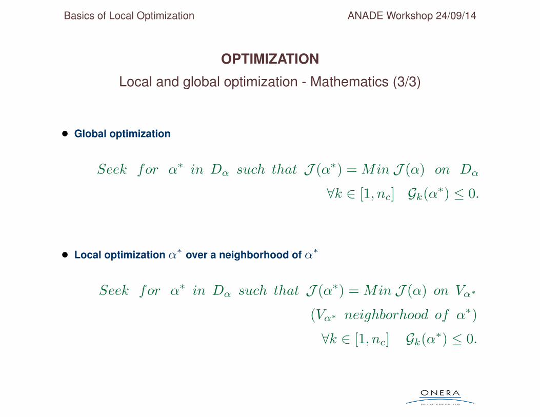
• Global optimization
Seek for α∗ in Dα such that J (α∗) = Min J (α) on Dα
∀k ∈ [1, nc] Gk(α∗) ≤ 0.
• Local optimization α∗ over a neighborhood of α∗
Seek for α∗ in Dα such that J (α∗) = Min J (α) on Vα∗
(Vα∗ neighborhood of α∗)
∀k ∈ [1, nc] Gk(α∗) ≤ 0.
Basics of Local Optimization ANADE Workshop 24/09/14
OPTIMIZATION
Local and global optimization - Mechanics (1/2)
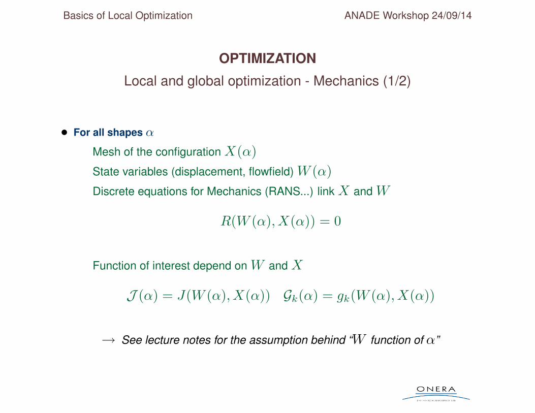
• For all shapes α
Mesh of the configuration X(α)State variables (displacement, flowfield) W (α)Discrete equations for Mechanics (RANS...) link X and W
R(W (α), X(α)) = 0
Function of interest depend on W and X
J (α) = J(W (α), X(α)) Gk(α) = gk(W (α), X(α))
→ See lecture notes for the assumption behind “W function of α”
Basics of Local Optimization ANADE Workshop 24/09/14
OPTIMIZATION
Local and global optimization - Mechanics (2/2)
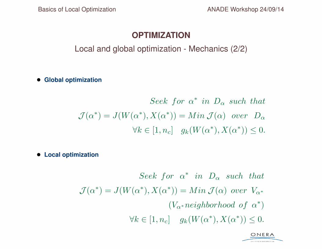
• Global optimization
Seek for α∗ in Dα such that
J (α∗) = J(W (α∗), X(α∗)) = Min J (α) over Dα
∀k ∈ [1, nc] gk(W (α∗), X(α∗)) ≤ 0.
• Local optimization
Seek for α∗ in Dα such that
J (α∗) = J(W (α∗), X(α∗)) = Min J (α) over Vα∗
(Vα∗neighborhood of α∗)
∀k ∈ [1, nc] gk(W (α∗), X(α∗)) ≤ 0.
Basics of Local Optimization ANADE Workshop 24/09/14
OPTIMIZATION
Classification of optimization Algorithms and associated subjects
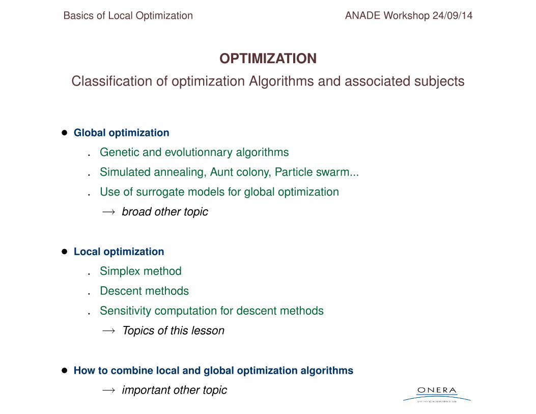
• Global optimization
. Genetic and evolutionnary algorithms
. Simulated annealing, Aunt colony, Particle swarm...
. Use of surrogate models for global optimization
→ broad other topic
• Local optimization
. Simplex method
. Descent methods
. Sensitivity computation for descent methods
→ Topics of this lesson
• How to combine local and global optimization algorithms
→ important other topic
Basics of Local Optimization ANADE Workshop 24/09/14
OPTIMIZATION
Outline of the lecture on local optimization
• The KKT (Karush-Kuhn-Tucker) conditions for local optimality
• Simplex method
• Descent methods
Basics of Local Optimization ANADE Workshop 24/09/14
KKT CONDITION FOR LOCAL OPTIMALITY
Outline of the lecture on local optimization
• The KKT (Karush-Kuhn-Tucker) conditions for local optimality
. KKT Conditions
. Solving KKT conditions in R2
• Simplex method
• Descent methods
Basics of Local Optimization ANADE Workshop 24/09/14
KKT CONDITION FOR LOCAL OPTIMALITY
Simple cases
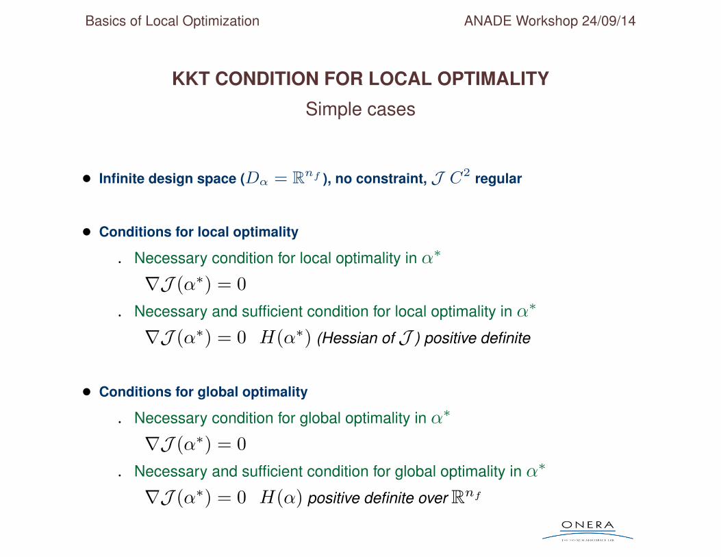
• Infinite design space (Dα = Rnf ), no constraint, J C2 regular
• Conditions for local optimality
. Necessary condition for local optimality in α∗
∇J (α∗) = 0. Necessary and sufficient condition for local optimality in α∗
∇J (α∗) = 0 H(α∗) (Hessian of J ) positive definite
• Conditions for global optimality
. Necessary condition for global optimality in α∗
∇J (α∗) = 0. Necessary and sufficient condition for global optimality in α∗
∇J (α∗) = 0 H(α) positive definite over Rnf
strudel
Basics of Local Optimization ANADE Workshop 24/09/14
KKT CONDITION FOR LOCAL OPTIMALITY
General case (1/2)
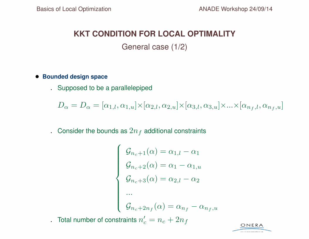
• Bounded design space
. Supposed to be a parallelepiped
Dα = Dα = [α1,l, α1,u]×[α2,l, α2,u]×[α3,l, α3,u]×...×[αnf ,l, αnf ,u]
. Consider the bounds as 2nf additional constraints
Gnc+1(α) = α1,l − α1
Gnc+2(α) = α1 − α1,u
Gnc+3(α) = α2,l − α2
...
Gnc+2nf(α) = αnf
− αnf ,u
. Total number of constraints n′c = nc + 2nf
Basics of Local Optimization ANADE Workshop 24/09/14
KKT CONDITION FOR LOCAL OPTIMALITY
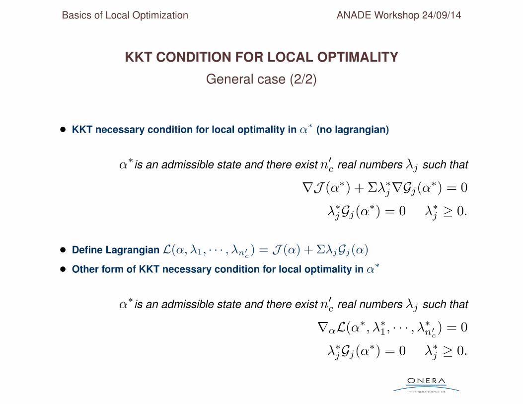
General case (2/2)
• KKT necessary condition for local optimality in α∗ (no lagrangian)
α∗is an admissible state and there exist n′c real numbers λj such that
∇J (α∗) + Σλ∗j∇Gj(α∗) = 0
λ∗jGj(α∗) = 0 λ∗j ≥ 0.
• Define Lagrangian L(α, λ1, · · · , λn′c) = J (α) + ΣλjGj(α)
• Other form of KKT necessary condition for local optimality in α∗
α∗is an admissible state and there exist n′c real numbers λj such that
∇αL(α∗, λ∗1, · · · , λ∗n′c) = 0
λ∗jGj(α∗) = 0 λ∗j ≥ 0.
Basics of Local Optimization ANADE Workshop 24/09/14
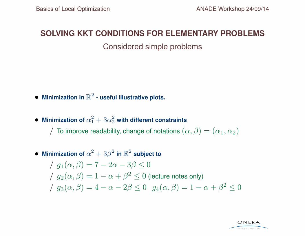
SOLVING KKT CONDITIONS FOR ELEMENTARY PROBLEMS
Considered simple problems
• Minimization in R2 - useful illustrative plots.
• Minimization of α21 + 3α2
2 with different constraints
/ To improve readability, change of notations (α, β) = (α1, α2)
• Minimization of α2 + 3β2 in R2 subject to
/ g1(α, β) = 7− 2α− 3β ≤ 0/ g2(α, β) = 1− α+ β2 ≤ 0 (lecture notes only)
/ g3(α, β) = 4− α− 2β ≤ 0 g4(α, β) = 1− α+ β2 ≤ 0
Basics of Local Optimization ANADE Workshop 24/09/14
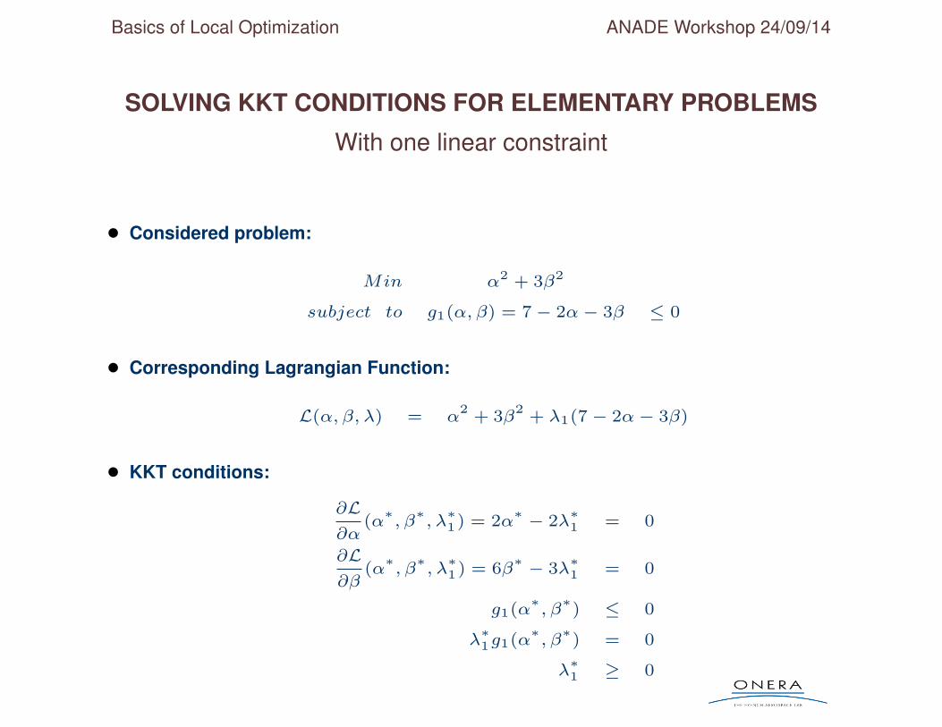
SOLVING KKT CONDITIONS FOR ELEMENTARY PROBLEMS
With one linear constraint
• Considered problem:
Min α2 + 3β2
subject to g1(α, β) = 7− 2α− 3β ≤ 0
• Corresponding Lagrangian Function:
L(α, β, λ) = α2
+ 3β2
+ λ1(7− 2α− 3β)
• KKT conditions:
∂L∂α
(α∗, β∗, λ∗1) = 2α
∗ − 2λ∗1 = 0
∂L∂β
(α∗, β∗, λ∗1) = 6β
∗ − 3λ∗1 = 0
g1(α∗, β∗) ≤ 0
λ∗1g1(α
∗, β∗) = 0
λ∗1 ≥ 0
Basics of Local Optimization ANADE Workshop 24/09/14
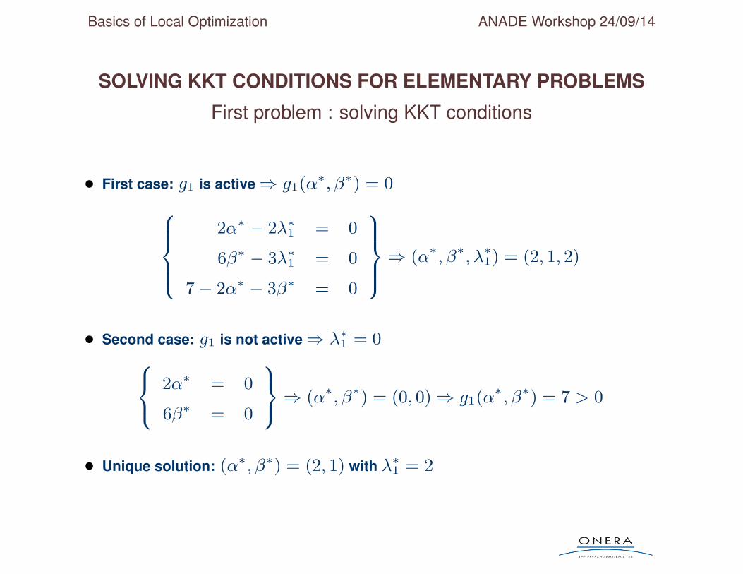
SOLVING KKT CONDITIONS FOR ELEMENTARY PROBLEMS
First problem : solving KKT conditions
• First case: g1 is active⇒ g1(α∗, β∗) = 08>><>>:2α∗ − 2λ∗1 = 0
6β∗ − 3λ∗1 = 0
7− 2α∗ − 3β∗ = 0
9>>=>>;⇒ (α∗, β∗, λ∗1) = (2, 1, 2)
• Second case: g1 is not active⇒ λ∗1 = 08<: 2α∗ = 0
6β∗ = 0
9=;⇒ (α∗, β∗) = (0, 0)⇒ g1(α∗, β∗) = 7 > 0
• Unique solution: (α∗, β∗) = (2, 1) with λ∗1 = 2
Basics of Local Optimization ANADE Workshop 24/09/14
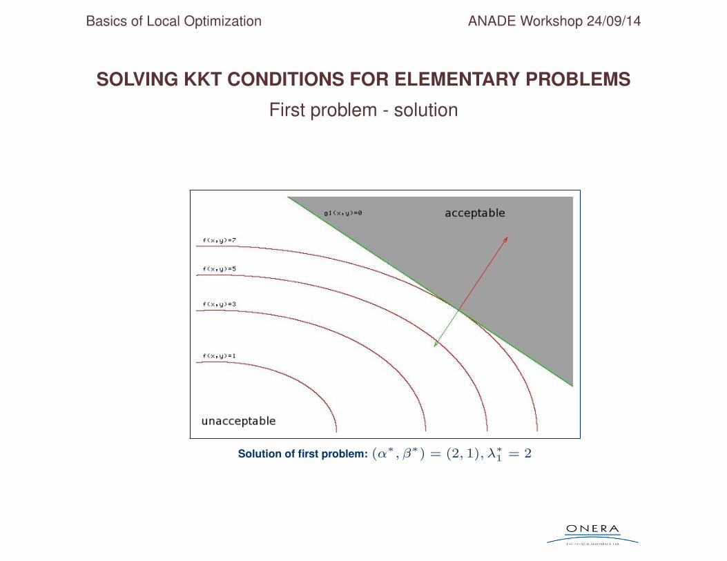
SOLVING KKT CONDITIONS FOR ELEMENTARY PROBLEMS
First problem - solution
Solution of first problem: (α∗, β∗) = (2, 1), λ∗1 = 2
Basics of Local Optimization ANADE Workshop 24/09/14
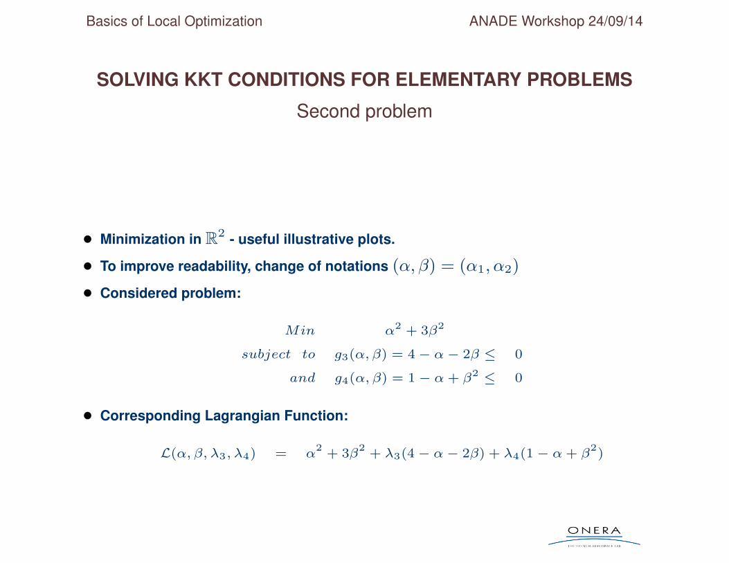
SOLVING KKT CONDITIONS FOR ELEMENTARY PROBLEMS
Second problem
• Minimization in R2 - useful illustrative plots.
• To improve readability, change of notations (α, β) = (α1, α2)
• Considered problem:
Min α2 + 3β2
subject to g3(α, β) = 4− α− 2β ≤ 0
and g4(α, β) = 1− α+ β2 ≤ 0
• Corresponding Lagrangian Function:
L(α, β, λ3, λ4) = α2
+ 3β2
+ λ3(4− α− 2β) + λ4(1− α+ β2)
Basics of Local Optimization ANADE Workshop 24/09/14
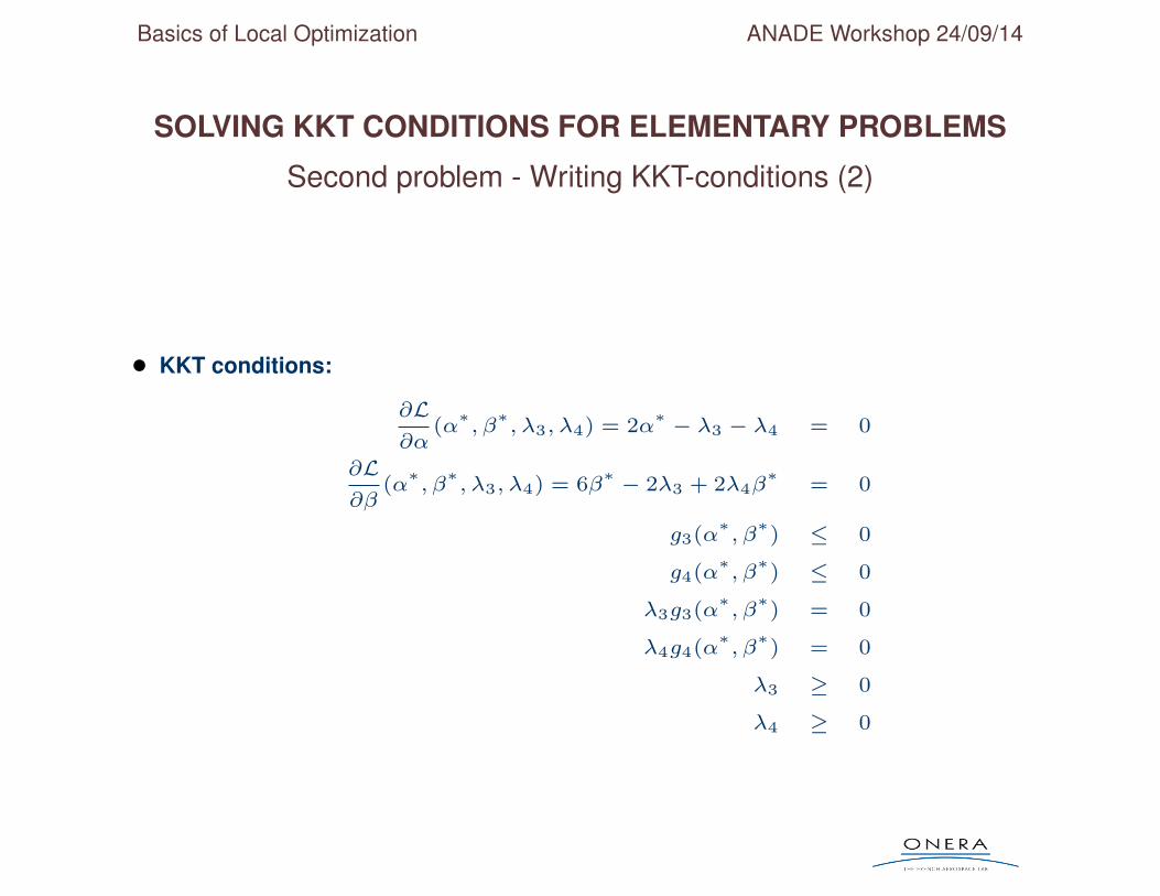
SOLVING KKT CONDITIONS FOR ELEMENTARY PROBLEMS
Second problem - Writing KKT-conditions (2)
• KKT conditions:
∂L∂α
(α∗, β∗, λ3, λ4) = 2α
∗ − λ3 − λ4 = 0
∂L∂β
(α∗, β∗, λ3, λ4) = 6β
∗ − 2λ3 + 2λ4β∗
= 0
g3(α∗, β∗) ≤ 0
g4(α∗, β∗) ≤ 0
λ3g3(α∗, β∗) = 0
λ4g4(α∗, β∗) = 0
λ3 ≥ 0
λ4 ≥ 0
Basics of Local Optimization ANADE Workshop 24/09/14
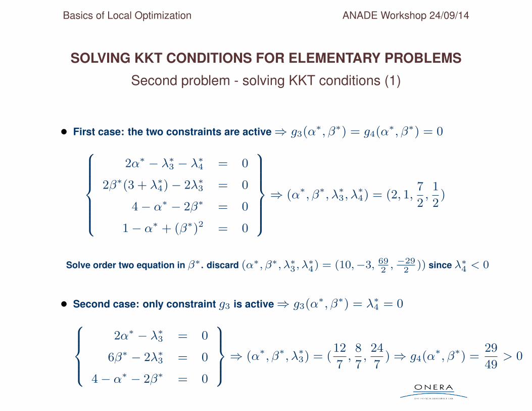
SOLVING KKT CONDITIONS FOR ELEMENTARY PROBLEMS
Second problem - solving KKT conditions (1)
• First case: the two constraints are active⇒ g3(α∗, β∗) = g4(α∗, β∗) = 08>>>>><>>>>>:2α∗ − λ∗3 − λ∗4 = 0
2β∗(3 + λ∗4)− 2λ∗3 = 0
4− α∗ − 2β∗ = 0
1− α∗ + (β∗)2 = 0
9>>>>>=>>>>>;⇒ (α∗, β∗, λ∗3, λ
∗4) = (2, 1,
7
2,
1
2)
Solve order two equation in β∗. discard (α∗, β∗, λ∗3, λ∗4) = (10,−3, 69
2, −29
2)) since λ∗4 < 0
• Second case: only constraint g3 is active⇒ g3(α∗, β∗) = λ∗4 = 08>><>>:2α∗ − λ∗3 = 0
6β∗ − 2λ∗3 = 0
4− α∗ − 2β∗ = 0
9>>=>>;⇒ (α∗, β∗, λ∗3) = (12
7,
8
7,
24
7)⇒ g4(α∗, β∗) =
29
49> 0
Basics of Local Optimization ANADE Workshop 24/09/14
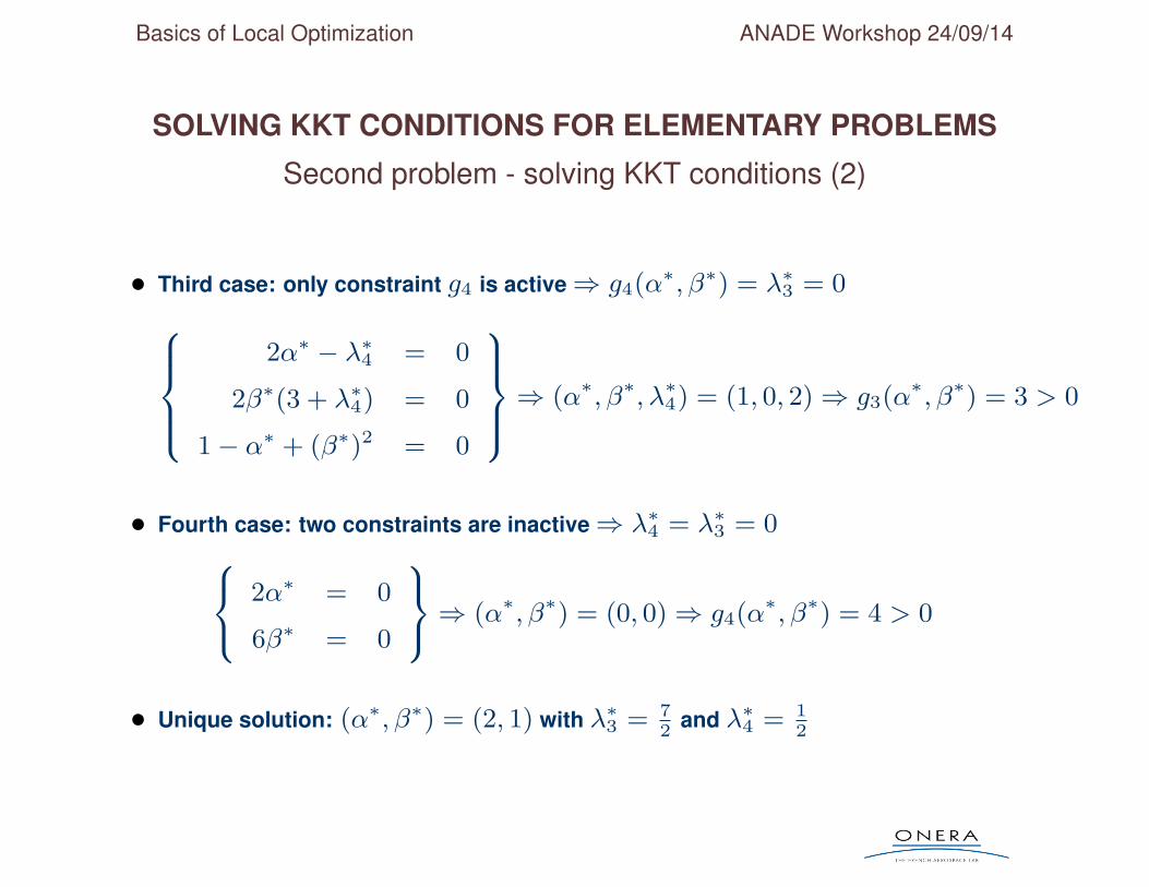
SOLVING KKT CONDITIONS FOR ELEMENTARY PROBLEMS
Second problem - solving KKT conditions (2)
• Third case: only constraint g4 is active⇒ g4(α∗, β∗) = λ∗3 = 08>><>>:2α∗ − λ∗4 = 0
2β∗(3 + λ∗4) = 0
1− α∗ + (β∗)2 = 0
9>>=>>;⇒ (α∗, β∗, λ∗4) = (1, 0, 2)⇒ g3(α∗, β∗) = 3 > 0
• Fourth case: two constraints are inactive⇒ λ∗4 = λ∗3 = 08<: 2α∗ = 0
6β∗ = 0
9=;⇒ (α∗, β∗) = (0, 0)⇒ g4(α∗, β∗) = 4 > 0
• Unique solution: (α∗, β∗) = (2, 1) with λ∗3 = 72
and λ∗4 = 12
Basics of Local Optimization ANADE Workshop 24/09/14
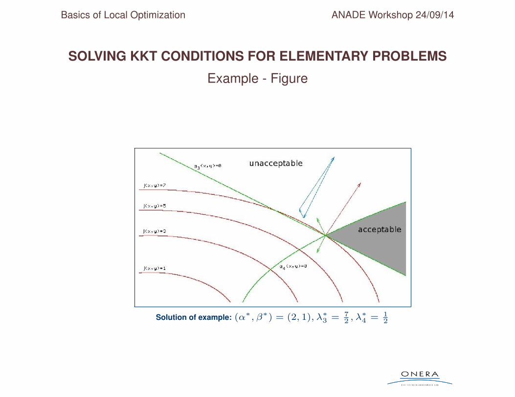
SOLVING KKT CONDITIONS FOR ELEMENTARY PROBLEMS
Example - Figure
Solution of example: (α∗, β∗) = (2, 1), λ∗3 = 72 , λ∗4 = 1
2
Basics of Local Optimization ANADE Workshop 24/09/14
SIMPLEX METHOD
Outline of the lecture on local optimization
• The KKT (Karush-Kuhn-Tucker) conditions for local optimality
• Simplex method
/ Definition of “simplex” or “polytop”
/ Transformation of the simplex
/ Algorithm
• Descent methods
Basics of Local Optimization ANADE Workshop 24/09/14
SIMPLEX METHOD
Introduction
• Deterministic and simple nonlinear local optimization algorithm:
/ Introduced by Nelder and Mead (1965)
/ "Direct method": uses only values of the objective function
/ Efficient (low memory and low computational cost), robust (very tolerant to
noise) and easy to code
• Based on the concept of “simplex” or “polytop”
/ Polytop = set of nd + 1 vertices (triangle in 2D, tetrahedron in 3D)
• Principle
/ Choice of an initial simplex
/ Successive transformation of simplex to adapt it to the objective function
Basics of Local Optimization ANADE Workshop 24/09/14
SIMPLEX METHOD
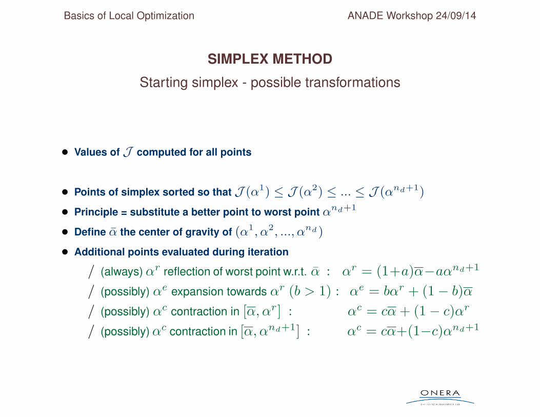
Starting simplex - possible transformations
• Values of J computed for all points
• Points of simplex sorted so that J (α1) ≤ J (α2) ≤ ... ≤ J (αnd+1)
• Principle = substitute a better point to worst point αnd+1
• Define α the center of gravity of (α1, α2, ..., αnd)
• Additional points evaluated during iteration
/ (always)αr reflection of worst point w.r.t. α : αr = (1+a)α−aαnd+1
/ (possibly) αe expansion towards αr (b > 1) : αe = bαr + (1− b)α/ (possibly) αc contraction in [α, αr] : αc = cα+ (1− c)αr
/ (possibly)αc contraction in [α, αnd+1] : αc = cα+(1−c)αnd+1
Basics of Local Optimization ANADE Workshop 24/09/14
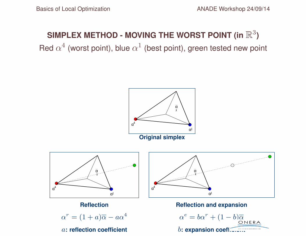
SIMPLEX METHOD - MOVING THE WORST POINT (in R3)
Red α4 (worst point), blue α1 (best point), green tested new point
α1α4
α
Original simplex
α1α4
α
α1α4
α
Reflection Reflection and expansion
αr = (1 + a)α− aα4 αe = bαr + (1− b)α
a: reflection coefficient b: expansion coefficient
Basics of Local Optimization ANADE Workshop 24/09/14
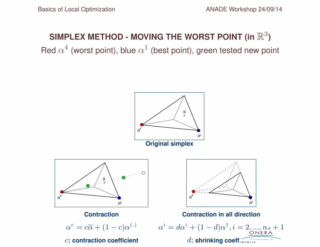
SIMPLEX METHOD - MOVING THE WORST POINT (in R3)
Red α4 (worst point), blue α1 (best point), green tested new point
α1α4
α
Original simplex
α1α4
α
α1α4
Contraction Contraction in all direction
αc = cα+ (1− c)α(.) αi = dαi + (1− d)α1, i = 2, ..., nd + 1
c: contraction coefficient d: shrinking coefficient
Basics of Local Optimization ANADE Workshop 24/09/14
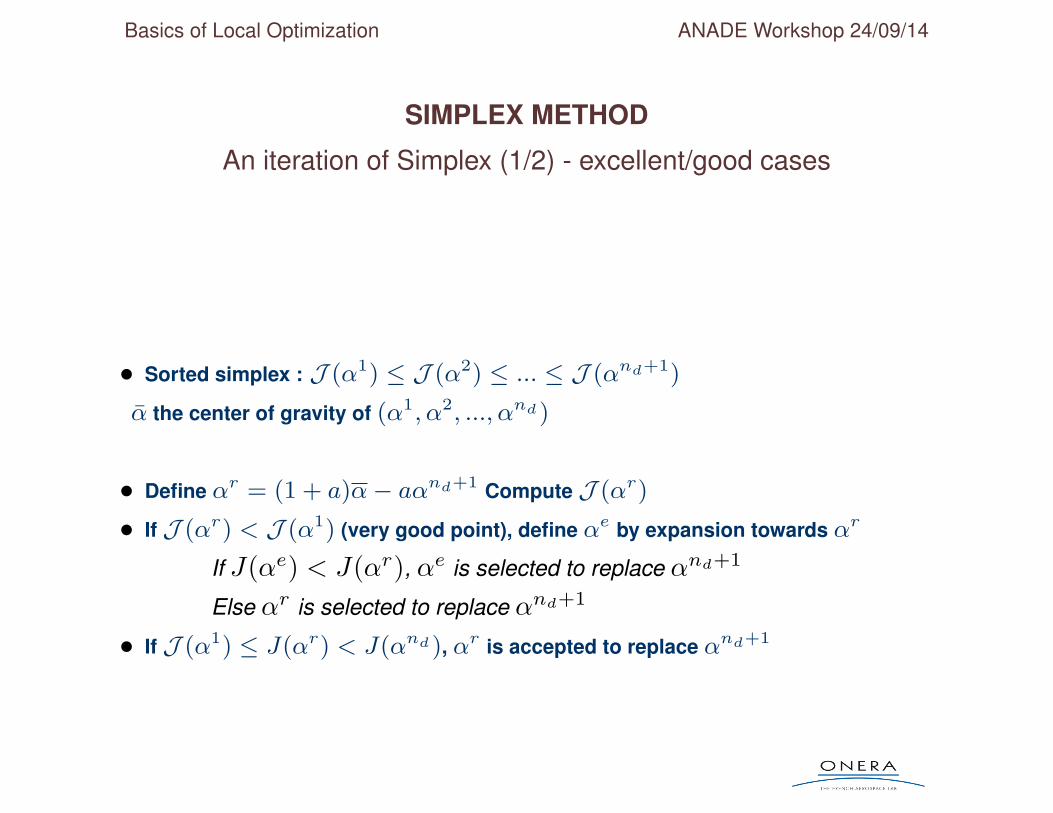
SIMPLEX METHOD
An iteration of Simplex (1/2) - excellent/good cases
• Sorted simplex : J (α1) ≤ J (α2) ≤ ... ≤ J (αnd+1)
α the center of gravity of (α1, α2, ..., αnd)
• Define αr = (1 + a)α− aαnd+1 Compute J (αr)
• If J (αr) < J (α1) (very good point), define αe by expansion towards αr
If J(αe) < J(αr), αe is selected to replace αnd+1
Else αr is selected to replace αnd+1
• If J (α1) ≤ J(αr) < J(αnd), αr is accepted to replace αnd+1
Basics of Local Optimization ANADE Workshop 24/09/14
SIMPLEX METHOD
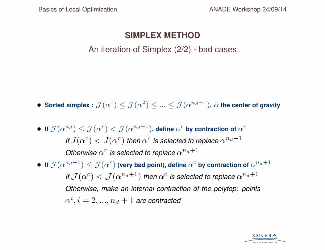
An iteration of Simplex (2/2) - bad cases
• Sorted simplex : J (α1) ≤ J (α2) ≤ ... ≤ J (αnd+1). α the center of gravity
• If J (αnd) ≤ J (αr) < J (αnd+1), define αc by contraction of αr
If J(αc) < J(αr) then αc is selected to replace αnd+1
Otherwise αr is selected to replace αnd+1
• If J (αnd+1) ≤ J (αr) (very bad point), define αc by contraction of αnd+1
If J (αc) < J (αnd+1) then αc is selected to replace αnd+1
Otherwise, make an internal contraction of the polytop: points
αi, i = 2, ..., nd + 1 are contracted
Basics of Local Optimization ANADE Workshop 24/09/14
SIMPLEX METHOD
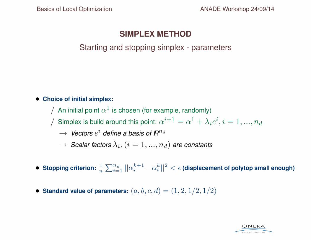
Starting and stopping simplex - parameters
• Choice of initial simplex:
/ An initial point α1 is chosen (for example, randomly)
/ Simplex is build around this point: αi+1 = α1 + λiei, i = 1, ..., nd
→ Vectors ei define a basis of IRnd
→ Scalar factors λi, (i = 1, ..., nd) are constants
• Stopping criterion: 1n
Pndi=1 ||α
k+1i −αki ||2 < ε (displacement of polytop small enough)
• Standard value of parameters: (a, b, c, d) = (1, 2, 1/2, 1/2)
Basics of Local Optimization ANADE Workshop 24/09/14
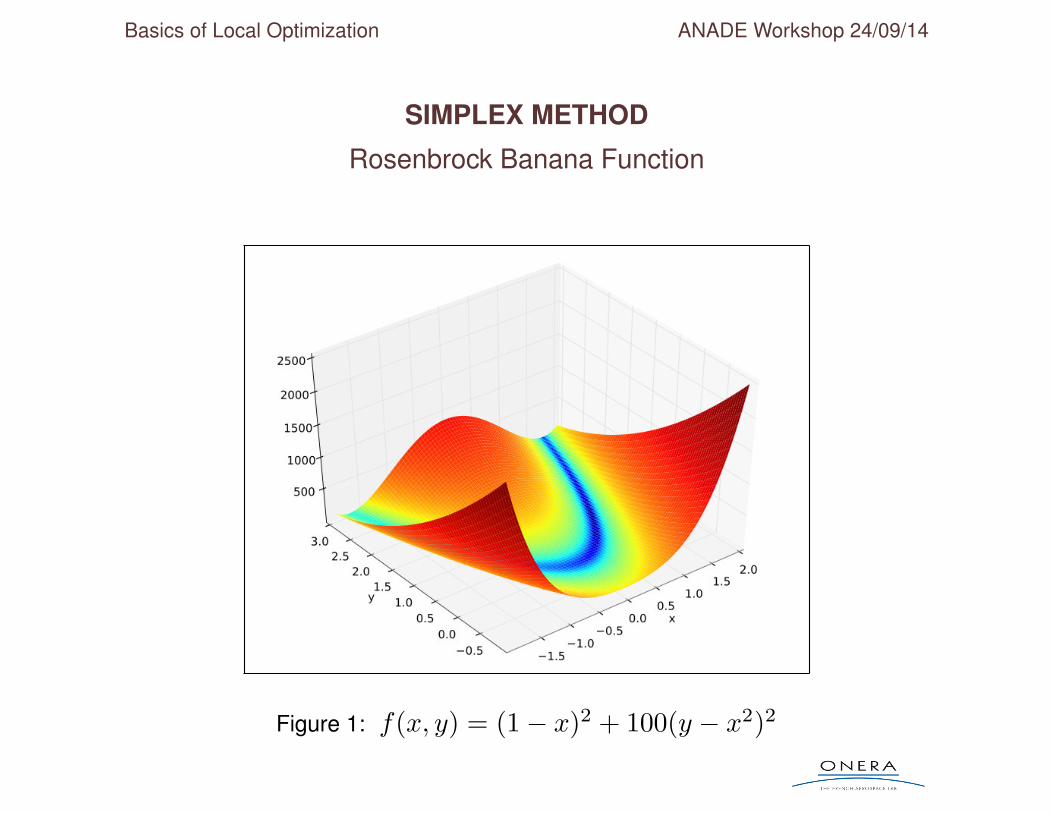
SIMPLEX METHOD
Rosenbrock Banana Function
Figure 1: f(x, y) = (1− x)2 + 100(y − x2)2
Basics of Local Optimization ANADE Workshop 24/09/14
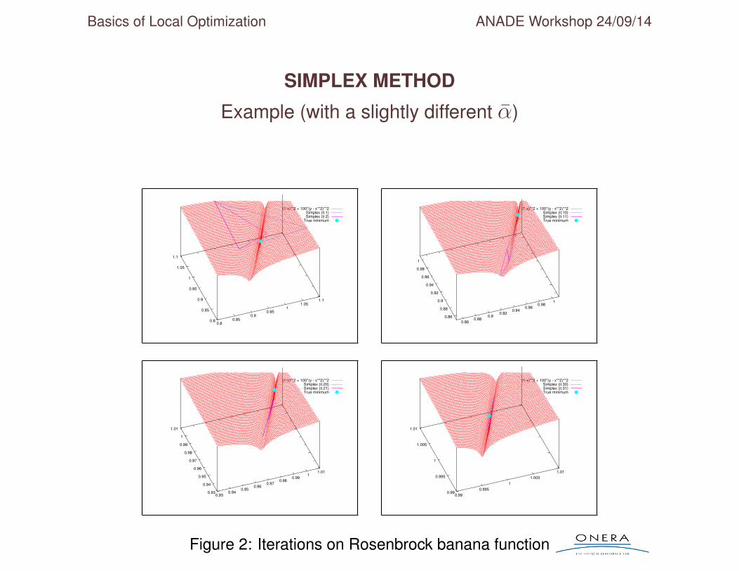
SIMPLEX METHOD
Example (with a slightly different α)
0.8 0.85
0.9 0.95
1 1.05
1.1
0.8
0.85
0.9
0.95
1
1.05
1.1
(1-x)**2 + 100*(y - x**2)**2Simplex (it.1)Simplex (it.2)
True minimum
0.86 0.88 0.9 0.92 0.94 0.96 0.98 1
0.86
0.88
0.9
0.92
0.94
0.96
0.98
1
(1-x)**2 + 100*(y - x**2)**2Simplex (it.10)Simplex (it.11)True minimum
0.93 0.94 0.95 0.96 0.97 0.98 0.99 1 1.01
0.93
0.94
0.95
0.96
0.97
0.98
0.99
1
1.01
(1-x)**2 + 100*(y - x**2)**2Simplex (it.20)Simplex (it.21)True minimum
0.99 0.995
1 1.005
1.01
0.99
0.995
1
1.005
1.01
(1-x)**2 + 100*(y - x**2)**2Simplex (it.30)Simplex (it.31)True minimum
Figure 2: Iterations on Rosenbrock banana function
Basics of Local Optimization ANADE Workshop 24/09/14
DESCENT METHODS
Sensitivity computation for descent methods
• The KKT (Karush-Kuhn-Tucker) conditions for local optimality
• Simplex method
• Descent methods
/ Line search (1D descent)
/ Unconstrained multi-D descent
/ Constrained multi-D descent
Basics of Local Optimization ANADE Workshop 24/09/14
LINE SEARCH
PRESENTATION
• One part of classical optimization algorithm (at iteration k):
/ Compute direction dk/ Compute step tk in direction dk (USE LINE-SEARCH)
/ Update current solution: αk+1 = αk + tkdk
• Objective of line-search:
/ Find step t which minimizes q(t) = J (αk + tdk)/ Use a reasonable number of function evaluations
Basics of Local Optimization ANADE Workshop 24/09/14
LINE SEARCH
List of methods
• Line search
/ Find step t which minimizes q(t) = J (αk + tdk)
• Academic line-search methods
/ Require large number of function/derivative evaluations
/ Methods of order 0 : golden number method...
/ Methods of order 1 : Wolfe line-search...
→ See lecture notes
• Other line-search methods
/ Robust and not too expensive
/ Polynomial approximations
→ Presented next slides
Basics of Local Optimization ANADE Workshop 24/09/14
LINE SEARCH
Academic methods - methods of order 0
• Naive method: search minimum by successive tries and search range refinement in the
vicinity of a local minimum
• Algorithm
/ Begin with a search interval [a0, b0]/ At each step k, choose two search points t−k and t+k in [ak, bk]/ q(t−k ) ≤ q(t+k )⇒ [ak, bk] = [ak−1, t
+k ]
/ q(t+k ) < q(t−k )⇒ [ak, bk] = [t−k , bk−1]/ Stop when |ak − bk| ≤ ε
• Need a strategy to choose search points
Basics of Local Optimization ANADE Workshop 24/09/14
LINE SEARCH
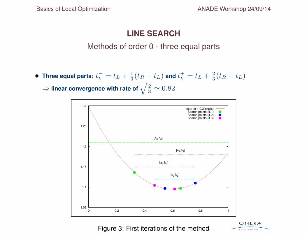
Methods of order 0 - three equal parts
• Three equal parts: t−k = tL + 13(tR − tL) and t+k = tL + 2
3(tR − tL)
⇒ linear convergence with rate ofq
23' 0.82
1.05
1.1
1.15
1.2
1.25
1.3
0 0.2 0.4 0.6 0.8 1
[a0,b0]
[a1,b1]
[a2,b2]
[a3,b3]
exp(-x) + 0.3*exp(x)Search points (it.1)Search points (it.2)Search points (it.3)
Figure 3: First iterations of the method
Basics of Local Optimization ANADE Workshop 24/09/14
LINE SEARCH
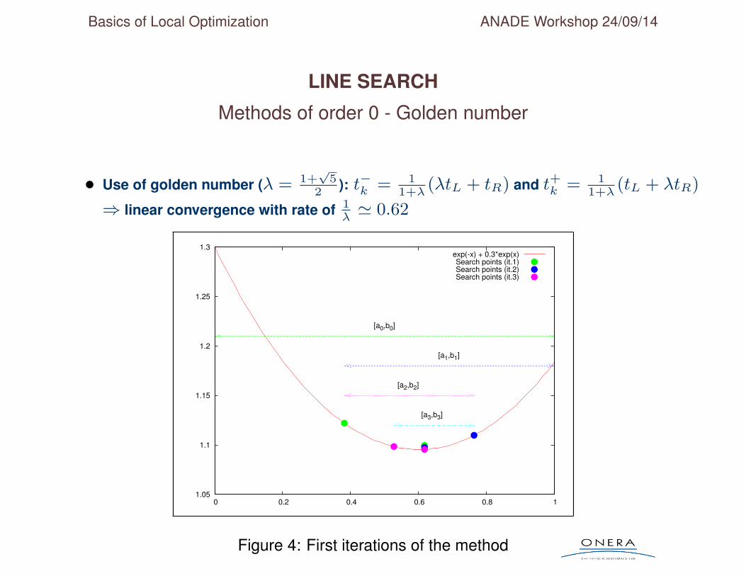
Methods of order 0 - Golden number
• Use of golden number (λ = 1+√
52
): t−k = 11+λ
(λtL + tR) and t+k = 11+λ
(tL + λtR)
⇒ linear convergence with rate of 1λ' 0.62
1.05
1.1
1.15
1.2
1.25
1.3
0 0.2 0.4 0.6 0.8 1
[a0,b0]
[a1,b1]
[a2,b2]
[a3,b3]
exp(-x) + 0.3*exp(x)Search points (it.1)Search points (it.2)Search points (it.3)
Figure 4: First iterations of the method
Basics of Local Optimization ANADE Workshop 24/09/14
LINE SEARCH
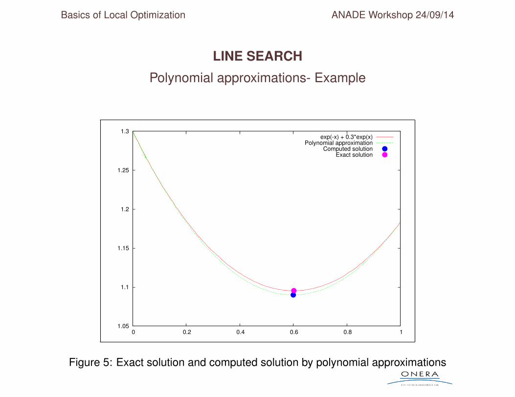
Polynomial approximations
• One ot the most effective techniques:
/ Requiring only a few function evaluations
/ Can lead to a very poor approximation for highly nonlinear functions
• Example: approximation with a polynomial of degree 2 q(t) = a0 + a1t+ a2t2
/ Evaluation of q and q′ at t0 = 0:⇒ (a0, a1) = (q(t0), q′(t0))/ Evaluation of q at an another point t1:⇒ a2 = q(t1)−a0−a1t1
t21
/ Identification of minimum: t∗ = −a12a2
• Approximation with a polynomial of degree n requires n − 1 function evaluations (in
addition to the evaluation of function and derivative in t0 = 0)
Basics of Local Optimization ANADE Workshop 24/09/14
LINE SEARCH
Polynomial approximations- Example
1.05
1.1
1.15
1.2
1.25
1.3
0 0.2 0.4 0.6 0.8 1
exp(-x) + 0.3*exp(x)Polynomial approximation
Computed solutionExact solution
Figure 5: Exact solution and computed solution by polynomial approximations
Basics of Local Optimization ANADE Workshop 24/09/14
UNCONSTRAINED MULTI-D DESCENT
Presentation
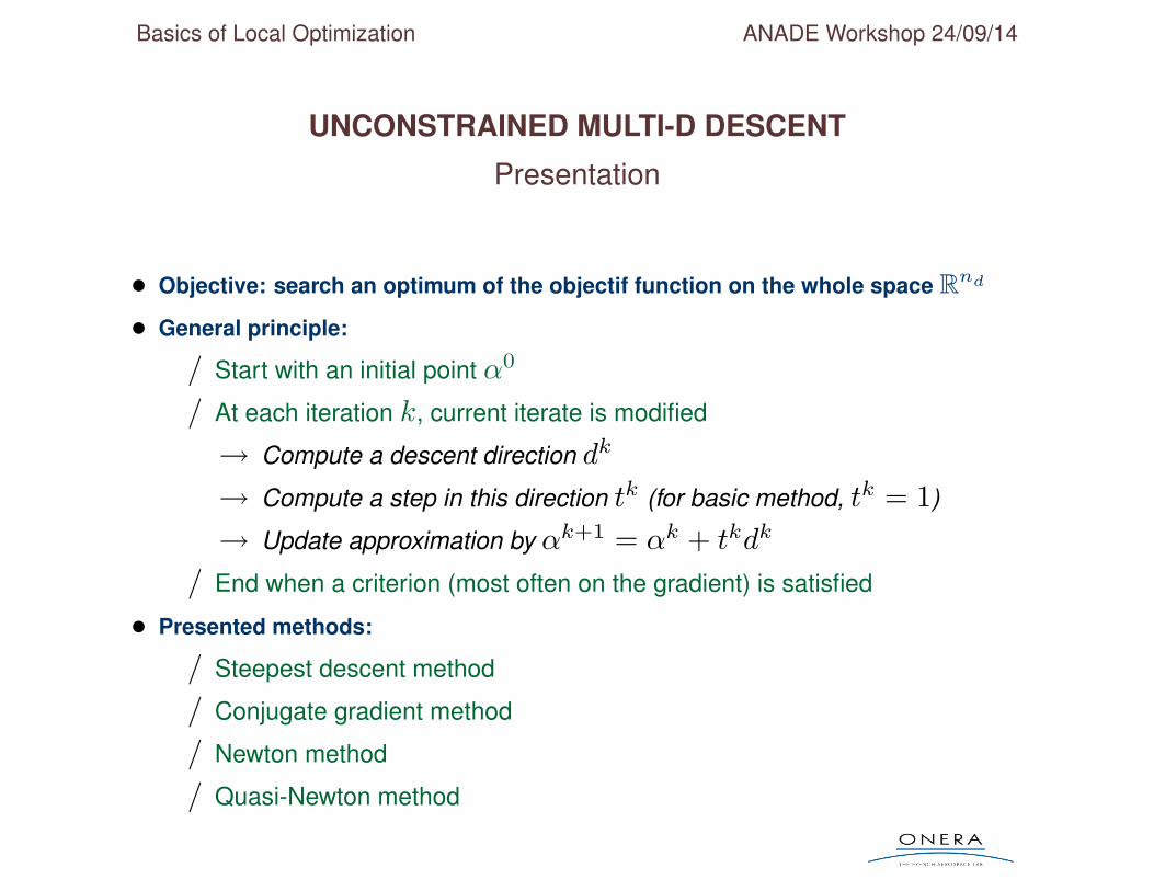
• Objective: search an optimum of the objectif function on the whole space Rnd
• General principle:
/ Start with an initial point α0
/ At each iteration k, current iterate is modified
→ Compute a descent direction dk
→ Compute a step in this direction tk (for basic method, tk = 1)
→ Update approximation by αk+1 = αk + tkdk
/ End when a criterion (most often on the gradient) is satisfied
• Presented methods:
/ Steepest descent method
/ Conjugate gradient method
/ Newton method
/ Quasi-Newton method
Basics of Local Optimization ANADE Workshop 24/09/14
UNCONSTRAINED MULTI-D DESCENT
Steepest descent method
• Most intuitive, basic method: dk = −∇J (αk) and tk = 1
/ Easy to implement
/ But short-sighted
/ Zig-zagging behaviour
• Optimal step version : dk = −∇J (αk) and optimal tk (line-search)
• Requires more information to be efficient
Basics of Local Optimization ANADE Workshop 24/09/14
UNCONSTRAINED MULTI-D DESCENT
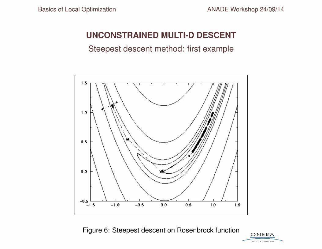
Steepest descent method: first example
Figure 6: Steepest descent on Rosenbrock function
Basics of Local Optimization ANADE Workshop 24/09/14
UNCONSTRAINED MULTI-D DESCENT
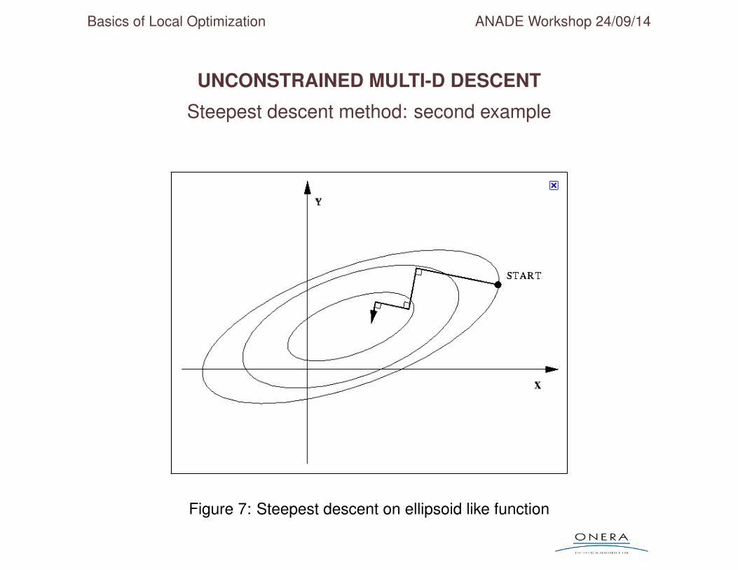
Steepest descent method: second example
Figure 7: Steepest descent on ellipsoid like function
Basics of Local Optimization ANADE Workshop 24/09/14
UNCONSTRAINED MULTI-D DESCENT
Conjugate gradient method (1/2)
• Minimization of (1/2(αTHα) + bTα) matrix H positive definite
/ one unique solution
/ also solution linear system Hα+ b = 0/ well-known linear algebra algorithm (Hestenes & Stiefel, 1952)
/ current descent direction combines function gradient and former direction
/ if steepest descent used, very sensitive to condition number of H
• Extensions
/ Linear algebra : different types of H (bi-CGSTAB, GMRES...)
/ Optimization : non quadratic functions
Basics of Local Optimization ANADE Workshop 24/09/14
UNCONSTRAINED MULTI-D DESCENT
Conjugate gradient method (2/2)
• Improve descent direction compared to steepest descent
/ Use direction descent dk conjugate to dk−1 in sense of H (like linear
algebra algorithm dTk−1Hdk = 0 )
dk = −∇J (αk) + βkdk−1 βk =
(∇J (αk)
)THdk−1
(dk−1)T Hdk−1
/ Use optimal step (line search) unlike linear algebra algorithm
/ Extend to non quadratic case:
• Fletcher-Reeves: βk = ‖∇J (αk)‖2‖∇J (αk−1)‖2
• Polak-Ribiere: βk = ‖∇J (αk)‖2 − (∇J (αk))T∇J (αk−1)
‖∇J (αk−1)‖2
• More efficient method require information about the second-order derivatives (Newton
method)
Basics of Local Optimization ANADE Workshop 24/09/14
UNCONSTRAINED MULTI-D DESCENT
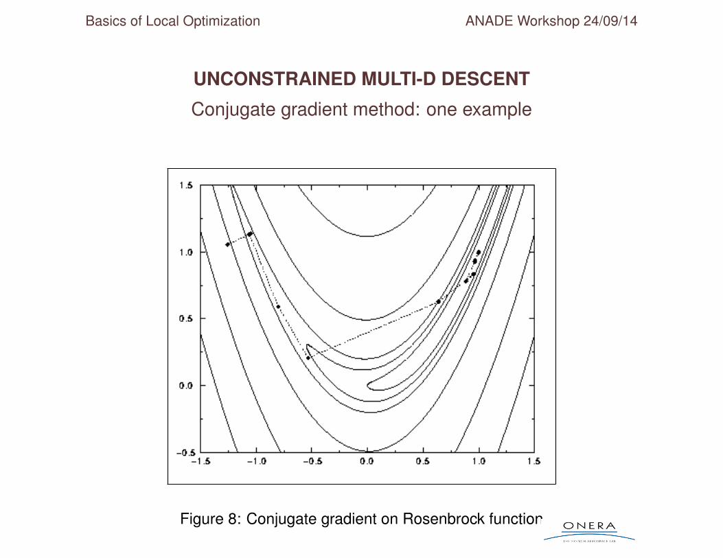
Conjugate gradient method: one example
Figure 8: Conjugate gradient on Rosenbrock function
Basics of Local Optimization ANADE Workshop 24/09/14
UNCONSTRAINED MULTI-D DESCENT
Newton method (1)
• Originally a method to find roots of equation z(α) = 0
/ Approximate z by linear expansion: z(αk + dk) ' z(αk) +∇z(αk)dk
/ Solve equation z(αk) +∇z(αk)dk = 0→ increment dk = −
[∇z(αk)
]−1z(αk)
/ Update current approximation: αk+1 = αk + dk
• Same method can be used as an optimization algorithm by searching roots of gradient of
the objective function
/ Descent direction is computed by: dk = −[∇2J (αk)
]−1∇J (αk)
Basics of Local Optimization ANADE Workshop 24/09/14
UNCONSTRAINED MULTI-D DESCENT
Newton method (2)
• Reminder α(k+1) = αk −ˆ∇2J (αk)
˜−1∇J (αk)
• Main advantage is the convergence in neighborhood of the solution
/ Superlinear in general
/ Quadratic (number of exact digits doubled at each iteration) if J has C3
regularity• Drawbacks
/ Hessian is required: explicit form unavailable in general and numerical com-
putation very expensive/ In high dimensional space, solution of linear system (at each iteration) CPU
demanding/ Violent divergence far from the optimal point
• Quasi-Newton methods developed to circumvent these drawbacks
Basics of Local Optimization ANADE Workshop 24/09/14
UNCONSTRAINED MULTI-D DESCENT
Quasi-Newton method
• Improvement over the Newton method based on two main ideas
/ Adding a line-search process to the algorithm:
→ At each iteration, compute an optimal step by minimizing
q(t) = J (αk + tdk) (Cf. line-search methods above)→ Hessian of the objective function needs to be positive
/ Approximate the inverse of the Hessian by a matrix H
• Algorithm:
/ Start from an initial point α0 with H initialized to a positive definite matrix
/ While ||∇J || > ε
→ Compute descent direction : dk = −Hk∇J (αk)→ Line-search (initialized t = 1)
→ Update current iterate: αk+1 = αk + tdk
→ Compute the new approximation Hk+1
Basics of Local Optimization ANADE Workshop 24/09/14
UNCONSTRAINED MULTI-D DESCENT
Quasi-Newton method: update H
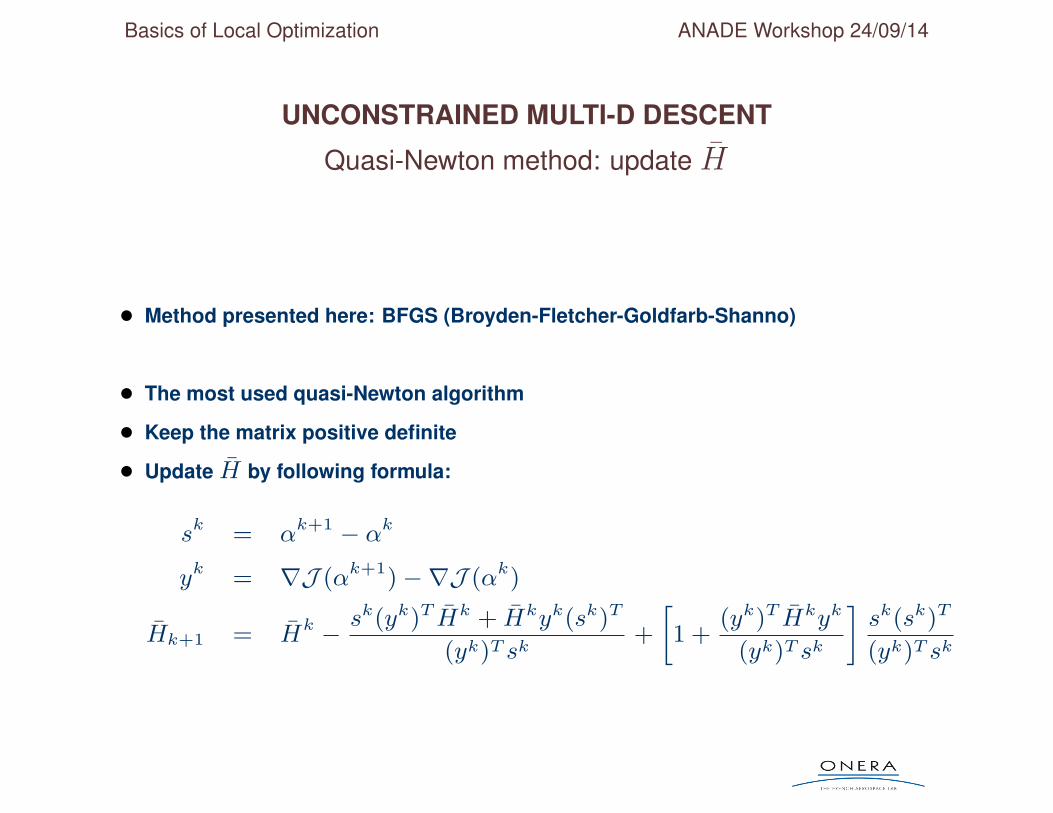
• Method presented here: BFGS (Broyden-Fletcher-Goldfarb-Shanno)
• The most used quasi-Newton algorithm
• Keep the matrix positive definite
• Update H by following formula:
sk = αk+1 − αk
yk = ∇J (αk+1)−∇J (αk)
Hk+1 = Hk − sk(yk)T Hk + Hkyk(sk)T
(yk)T sk+
»1 +
(yk)T Hkyk
(yk)T sk
–sk(sk)T
(yk)T sk
Basics of Local Optimization ANADE Workshop 24/09/14
UNCONSTRAINED MULTI-D DESCENT
Quasi-Newton method: one example
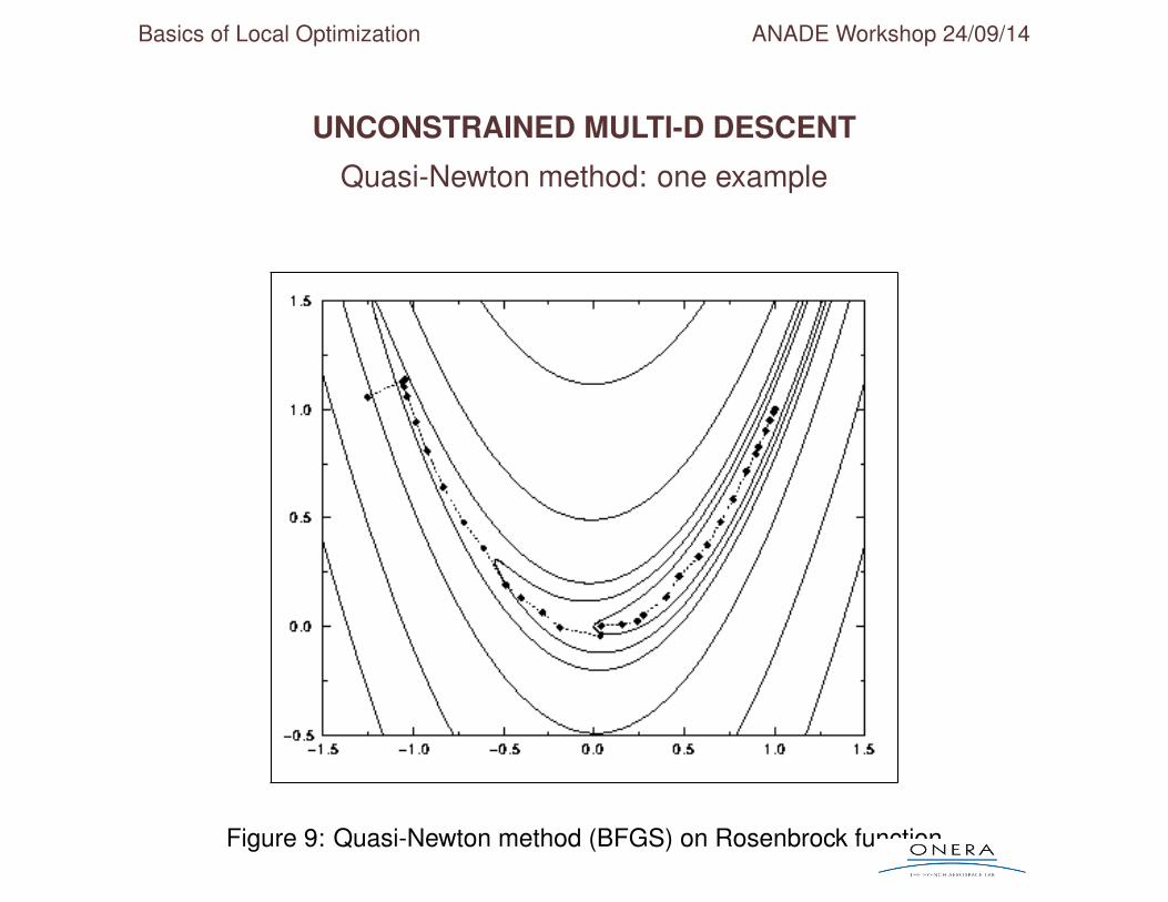
Figure 9: Quasi-Newton method (BFGS) on Rosenbrock function
Basics of Local Optimization ANADE Workshop 24/09/14
CONSTRAINED MULTI-D DESCENT
Reminder
• Solve the mathematical problem defined at the beginning of the talk
• Local optimization problem :
Seek for α∗ in Dα such that J (α∗) = Min J (α) on Vα∗
(Vα∗ neighborhood of α∗)
∀k ∈ [1, nc] Gk(α∗) ≤ 0.
• Restricted to differentiable functions
• Four methods
/ Sequential linear programming→ see lecture notes
/ Method of centers→ see lecture notes
/ Feasible direction method
/ Sequential quadratic programming
Basics of Local Optimization ANADE Workshop 24/09/14
CONSTRAINED MULTI-D DESCENT
Method of feasible direction (1/4)
• Two-step “non-linear” algorithm
/ Search for descent direction (taking into account non-linearity of active con-
straints)/ Line-search along descent-direction
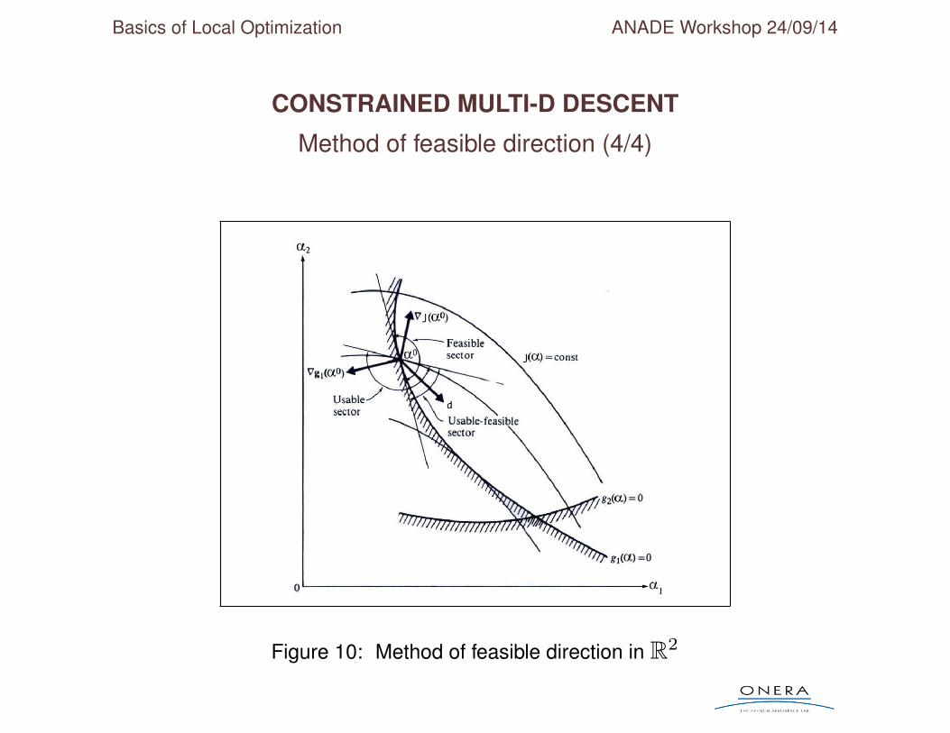
• Definition of descent direction
/ Goal find best possible descent direction, avoiding following “trap” :
→ In R2, current point α0, objective J , one CONVEX ACTIVE
constraint G1.
The solution of “Find d (a priori bounded) minimizing
∇J (α0).d subject to ∇G1(α0).d < 0” leads to inadmissi-
ble α1 (see plot of slide N+3)
Basics of Local Optimization ANADE Workshop 24/09/14
CONSTRAINED MULTI-D DESCENT
Method of feasible direction (2/4)
• Definition of descent direction d
• Avoid trap described on previous slide
/ Good requirement associated to an active convex constraint is
∇G1(α0).d+ θj < 0 θj > 0• Need to link the decrease of J and Gj along d
• “Good” feasible direction search
/ Maximize β, find dk (a priori bounded), such that
. ∇J (α0).dk + β ≤ 0.
. ∇Gj(α0).dk + θjβ ≤ 0. ∀j/Gj(α0) = 0
Basics of Local Optimization ANADE Workshop 24/09/14
CONSTRAINED MULTI-D DESCENT
Method of feasible direction (3/4)
• Algorithm :
/ Set k = 0; an initial iterate α0 and a stopping tolerance ε are given.
/ WHILE KKT-conditions not satisfied
Maximize β, find dk (a priori bounded), such that
. ∇J (αk).dk + β ≤ 0.
. ∇Gj(αk).dk + θjβ ≤ 0. ∀j/Gj(αk) = 0Minimize q(t) = J(αk + tdk) (One dimensional search)
Update αk+1 = αk + tdk
Set k = k + 1/ END WHILE
Basics of Local Optimization ANADE Workshop 24/09/14
CONSTRAINED MULTI-D DESCENT
Method of feasible direction (4/4)
Figure 10: Method of feasible direction in R2
Basics of Local Optimization ANADE Workshop 24/09/14
CONSTRAINED MULTI-D DESCENT
Sequential quadratic programming (SQP) (1/2)
• Solve a sequence of quadratic minimization with linear constraints
• Quadratic minimization of Q(d) = J (αk) +∇J (αk).d+ 12dTBd
/ B approximate Hessian matrix
• Set of linear constraints∇Gj(αk).d+ δjGj(αk) ≤ 0. j = 1, nc
/ δj=1 for strictly respected constraint
Gj(αk) < 0 value of the constraint may increase
/ δj ∈ [0, 1] for violated constraints
Gj(αk) > 0 Forces decrease of (first-order expansion of) Gj
Basics of Local Optimization ANADE Workshop 24/09/14
CONSTRAINED MULTI-D DESCENT
Sequential quadratic programming (SQP) (2/2)
• Algorithm :
/ Set k = 0; an initial iterate α0, a stopping tolerance ε, and initial approxi-
mate Hessian matrix B0 are given./ WHILE KKT-conditions not satisfied
Find dk which
. minimizes J (αk) +∇J (αk).d+ 12dTBkd
. subject to∇Gj(αk).d+ δjGj(αk) ≤ 0. j = 1, ncUpdate αk+1 = αk + dk
Build Bk+1 (for example, from BFGS formula)
Set k = k + 1/ END WHILE