local, unconstrained function optimization

Local, Unconstrained FunctionOptimization

COMPSCI 371D — Machine Learning

COMPSCI 371D — Machine Learning Local, Unconstrained Function Optimization 1 / 25

Outline

1 Motivation and Scope

2 First Order Methods

3 Gradient, Hessian, and Convexity

4 Gradient Descent

5 Stochastic Gradient Descent

6 Step Size Selection Methods

7 Termination

8 Is Gradient Descent a Good Strategy?


Motivation and Scope


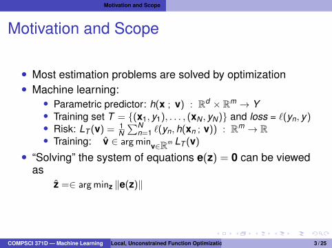
• Most estimation problems are solved by optimization• Machine learning:

• Parametric predictor: h(x ; v) : Rd × Rm → Y• Training set T = {(x1, y1), . . . , (xN , yN)} and loss = `(yn, y)• Risk: LT (v) = 1

N∑N

n=1 `(yn,h(xn ; v)) : Rm → R• Training: v ∈ argminv∈Rm LT (v)

• “Solving” the system of equations e(z) = 0 can be viewedas

z =∈ argminz ‖e(z)‖



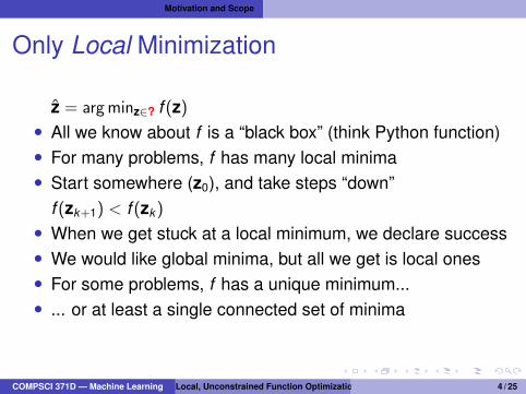
Only Local Minimization

z = argminz∈? f (z)• All we know about f is a “black box” (think Python function)• For many problems, f has many local minima• Start somewhere (z0), and take steps “down”

f (zk+1) < f (zk)

• When we get stuck at a local minimum, we declare success• We would like global minima, but all we get is local ones• For some problems, f has a unique minimum...• ... or at least a single connected set of minima


First Order Methods

Gradient

∇f (z) = ∂f∂z =

∂f∂z1...∂f∂zm

z ∈ Rm with m possibly very large• If ∇f (z) exists everywhere, the condition ∇f (z) = 0

is necessary and sufficient for a stationary point(max, min, or saddle)• Warning: only necessary for a minimum!• Reduces to first derivative when f : R→ R


First Order Methods

First Order Taylor Expansionf (z) ≈ g1(z) = f (z0) + [∇f (z0)]

T (z− z0)

approximates f (z) near z0 with a (hyper)plane through z0

z1

z2

f(z)

z0

∇f (z0) points to direction of steepest increase of f at z0

• If we want to find z1 where f (z1) < f (z0), going along−∇f (z0) seems promising• This is the general idea of gradient descent


Gradient, Hessian, and Convexity

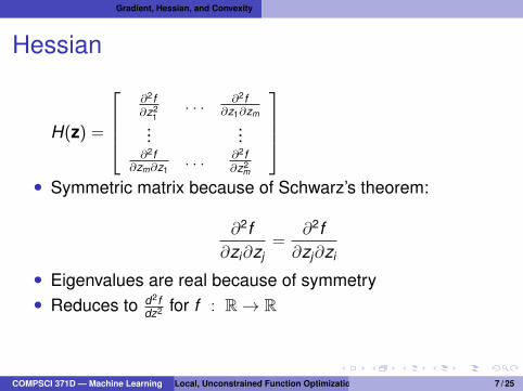
Hessian

H(z) =

∂2f∂z2

1. . . ∂2f

∂z1∂zm

......

∂2f∂zm∂z1

. . . ∂2f∂z2

m

• Symmetric matrix because of Schwarz’s theorem:

∂2f∂zi∂zj

=∂2f∂zj∂zi

• Eigenvalues are real because of symmetry• Reduces to d2f

dz2 for f : R→ R



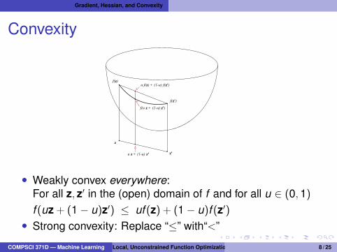
Convexity

z

z'u z + (1-u) z'

f(u z + (1-u) z')

u f(z) + (1-u) f(z')

f(z')

f(z)

• Weakly convex everywhere:For all z, z′ in the (open) domain of f and for all u ∈ (0,1)f (uz + (1− u)z′) ≤ uf (z) + (1− u)f (z′)• Strong convexity: Replace “≤” with“<”



Convexity and Hessian

• Things become operational for twice-differentiable functions• The function f (z) is weakly convex everywhere iff H(z) < 0

for all z• “<” means positive semidefinite:

vT H(z)v ≥ 0 for all v ∈ Rm

• Above is definition of H(z) < 0• To check computationally: All eigenvalues are nonnegative• H(z) < 0 reduces to d2f

dz2 ≥ 0 for f : R→ R• Analogous result for strong convexity: H(z) � 0, that is,

vT H(z)v > 0 for all v ∈ Rm

(All eigenvalues are positive)



Local Convexity• The function f is convex at z0 if it is convex everywhere in

some open neighborhood of z0

• Convexity at z0 is not equivalent to H(z0) � 0 or H(z0) < 0• H(z0) � 0 is only sufficient for strong convexity at z0

• Example: f (z) = x2/2 is strongly convex at z0 = 0 andHf (z0) = 1 � 0

• Example: f (z) = x4 is strongly convex at z0 = 0 butHf (z0) = 0 < 0 (so Hf (z0) = 1 � 0 is not necessary for strongconvexity at z0)

• For weak convexity at z0 we need to check that H(z) < 0 forevery z in some open neighborhood of z0

• Example: f (z) = z3/6, for which we have Hf (z) = z• Hf (0) < 0 (and in fact Hf (0) = 0)• However, every neighborhood of z0 = 0 has points (any

z < 0) where Hf (z) ≺ 0• So f (z) is not (even weakly) convex at z0 = 0



Some Uses of Convexity

• If ∇f (z) = 0 and f is convex at z then z is a minimum (asopposed to a maximum or a saddle)• If f is globally convex then the value of the minimum is

unique and minima form a convex set• Faster optimization methods can be used when

f : Rm → R is convex and m is not too large



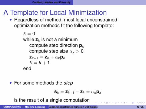
A Template for Local Minimization• Regardless of method, most local unconstrained

optimization methods fit the following template:

k = 0while zk is not a minimum

compute step direction pk

compute step size αk > 0zk+1 = zk + αkpk

k = k + 1end

• For some methods the step

sk = zk+1 − zk = αkpk

is the result of a single computationCOMPSCI 371D — Machine Learning Local, Unconstrained Function Optimization 12 / 25


Design Decisions

k = 0while zk is not a minimum

compute step direction pk

compute step size αk > 0zk+1 = zk + αkpk

k = k + 1end

• In what direction toproceed (pk )• How long a step to take

in that direction (αk )• When to stop (“while zk

is not a minimum”)• Different decisions lead

to different methods


Gradient Descent

Gradient Descent

• In what direction to proceed: pk = −∇f (zk)

• “Gradient descent”• Problem reduces to one dimension:

h(α) = f (zk + αpk)

• α = 0⇔ z = zk

• Find α = αk > 0 such thatf (zk + αkpk) < f (zk)

• How to find αk?


Stochastic Gradient Descent

Stochastic Gradient Descent• A special case of gradient descent, SGD works for

averages of many terms (N very large):

f (z) =1N

N∑n=1

φn(z)

• Computing ∇f (zk) is too expensive• Partition B = {1, . . . ,N} into J random mini-batches Bj

each of about equal size

f (z) ≈ fj(z) =1|Bj |

∑n∈Bj

φn(z) ⇒ ∇f (z) ≈ ∇fj(z) .

• Mini-batch gradients are correct on average


Stochastic Gradient Descent

SGD and Mini-Batch Size

• SGD iteration: zk+1 = zk − αk∇fj(zk)

• Mini-batch gradients are correct on average• One cycle through all the mini-batches is an epoch• Repeatedly cycle through all the data

(Scramble data before each epoch)• Asymptotic convergence can be proven with suitable

step-size schedule• Small batches⇒ low storage but high gradient variance• Make batches as big as will fit in memory for minimal

variance• In deep learning, memory is GPU memory


Step Size Selection Methods

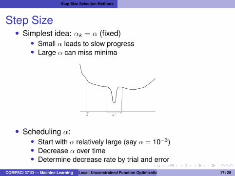
Step Size• Simplest idea: αk = α (fixed)

• Small α leads to slow progress• Large α can miss minima

α α᾽

• Scheduling α:• Start with α relatively large (say α = 10−3)• Decrease α over time• Determine decrease rate by trial and error



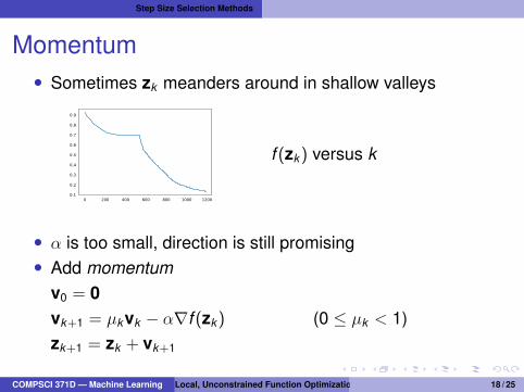
Momentum• Sometimes zk meanders around in shallow valleys

0 200 400 600 800 1000 12000.1

0.2

0.3

0.4

0.5

0.6

0.7

0.8

0.9

f (zk) versus k

• α is too small, direction is still promising• Add momentum

v0 = 0vk+1 = µkvk − α∇f (zk) (0 ≤ µk < 1)zk+1 = zk + vk+1



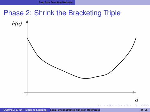
Line Search

• Find a local minimum in the search direction pk

h(α) = f (zk + αpk), a one-dimensional problem• Bracketing triple:• a < b < c, h(a) ≥ h(b), h(b) ≤ h(c)• Contains a (local) minimum!• Split the bigger of [a,b] and [b, c] in half with a point u• Find a new, narrower bracketing triple involving u and two

out of a,b, c• Stop when the bracket is narrow enough (say, 10−6)• Pinned down a minimum to within 10−6



Phase 1: Find a Bracketing Triple

α

h(α)



Phase 2: Shrink the Bracketing Triple

α

h(α)



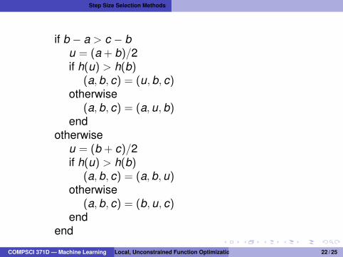
if b − a > c − bu = (a + b)/2if h(u) > h(b)

(a,b, c) = (u,b, c)otherwise

(a,b, c) = (a,u,b)end

otherwiseu = (b + c)/2if h(u) > h(b)

(a,b, c) = (a,b,u)otherwise

(a,b, c) = (b,u, c)end

end


Termination

Termination

• Are we still making “significant progress”?• Check f (zk−1)− f (zk)? (We want this to be strictly positive)• Check ‖zk−1 − zk‖ ? (We want this to be large enough)• Second is more stringent close the the minimum

because ∇f (z) ≈ 0• Stop when ‖zk−1 − zk‖ < δ


Is Gradient Descent a Good Strategy?

Is Gradient Descent a Good Strategy?• “We are going in the direction of fastest descent”• “We choose an optimal step size by line search”• “Must be good, no?” Not so fast!• An example for which we know the answer:

f (z) = c + aT z + 12zT Qz

Q < 0 (convex paraboloid)• All smooth functions look like this close enough to z∗

z*

isocontours


Is Gradient Descent a Good Strategy?

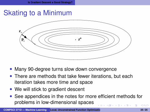
Skating to a Minimum

z 0

z*p0

• Many 90-degree turns slow down convergence• There are methods that take fewer iterations, but each

iteration takes more time and space• We will stick to gradient descent• See appendices in the notes for more efficient methods for

problems in low-dimensional spacesCOMPSCI 371D — Machine Learning Local, Unconstrained Function Optimization 25 / 25

local, unconstrained function optimization

Documents