Computational Economics and Finance

Part IV:

Unconstrained Optimization

Spring 2015

Outline

Comparison Methods

Optimality Conditions

Newton’s Method

Line Search Methods

Trust Region Methods

2

Unconstrained Optimization

Unconstrained minimization problem

minx∈Rn

f(x)

where f : Rn → R is the objective function

Optimal solution x∗ satisfies f(x∗) ≤ f(x) for all x ∈ Rn

Minimizer x∗, minimum f(x∗)

Equivalence between maximization and minimization problems

max f(x) = −min−f(x)

Very difficult problem in general

3

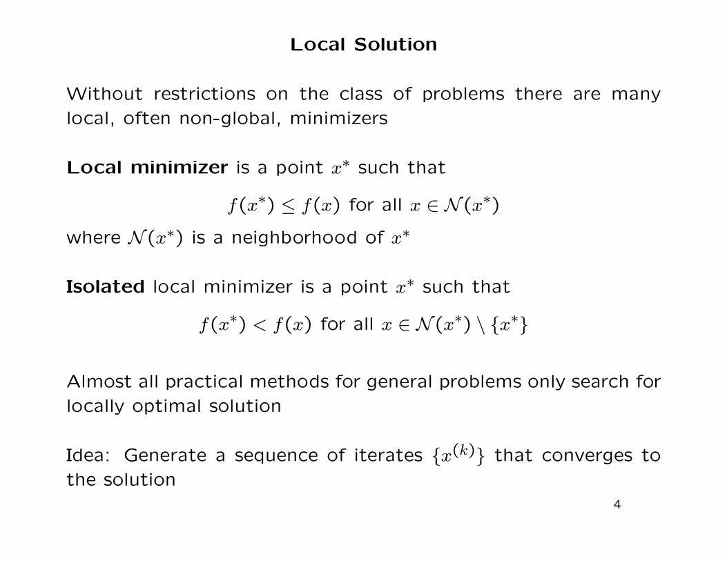
Local Solution

Without restrictions on the class of problems there are many

local, often non-global, minimizers

Local minimizer is a point x∗ such that

f(x∗) ≤ f(x) for all x ∈ N (x∗)

where N (x∗) is a neighborhood of x∗

Isolated local minimizer is a point x∗ such that

f(x∗) < f(x) for all x ∈ N (x∗) \ {x∗}

Almost all practical methods for general problems only search for

locally optimal solution

Idea: Generate a sequence of iterates {x(k)} that converges to

the solution4

Grid Search

Grid search method:

Specify a grid of points {xg}Gg=1, evaluate f at these points, and

pick the minimum

May indicate potential regions for minimizer and guide applica-

tion of more advanced methods

Should always be done as an initial step

Grid search is an example of a comparison method, only re-

quires comparison of function values

5

Comparison Method for One-dimensional Optimization

Bracketing search method: Golden ratio search

Find local minimum of function f on interval [a, b]

Select two interior points c, d, such that a < c < d < b

Case 1: f(c) ≤ f(d) minimum must lie in [a, d]replace b with d, new interval [a, d]

Case 2: f(c) > f(d) minimum must lie in [c, b]replace a with c, new interval [c, b]

Now repeat the iteration on the new interval

Question: How to choose c and d?

6

Choosing Points

Select c and d such that the intervals [a, c] and [d, b] have the

same length, so c− a = b− d

c = a+ (1− r)(b− a) = ra+ (1− r)b

d = b− (1− r)(b− a) = (1− r)a+ rb

where 12 < r < 1 to ensure c < d

One of the old interior points will be an endpoint of the new

interval; for efficiency, use the other interior point also as an

interior point for the new subinterval; so in each iteration only

one new interior point and only one new function evaluation is

needed

If f(c) ≤ f(d) then these conditions require

d− a

b− a=

c− a

d− a

7

Golden Ratio

d−ab−a = c−a

d−a

⇐⇒ r(b−a)b−a = (1−r)(b−a)

r(b−a)

⇐⇒ r = (1−r)r

⇐⇒ r2 = 1− r

⇐⇒ r2 + r − 1 = 0

⇐⇒ r = −1±√5

2

and thus r is the golden ratio,

r =−1+

√5

2≈ 0.618034

Interior points

c = a+ (1− r)(b− a)

d = a+ r(b− a)

8

Examples

Miranda/Fackler Figure 4.1: f(x) = x · cos(x2)

Palgrave Example 1: f(x) = ln(x) + 2 · ln(1− x)

Mathematica: Subroutine GoldenSearch

Matlab: CompEcon Toolbox routine golden

9

Comparison Method for Multivariate Functions

No simple bracketing of a minimum in more than one dimension

Prominent comparison method used in economics:

Nelder-Mead (simplex) method

Goal of Nelder-Mead method:

Find a simplex containing a (local) minimizer x∗ = (x∗1, x∗2, . . . , x

∗n)

of the function f : Rn → R

Simplex is the convex hull of n+1 affinely independent points,

that is, of n + 1 points in general position (n-dimensional ana-

logue of a triangle in two dimensions)

10

One Iteration of Nelder-Mead Method

Simplex {x1, . . . , xn+1} with vertices x1, x2, . . ., xn+1 is given

Reorder vertices such that f(xi) ≤ f(xi+1), i = 1, . . . , n

“Worst” point with highest objective function value is xn+1

Goal: replace xn+1 with a new vertex

One iteration of Nelder-Mead method can be one of four possible

steps:

reflect, expand, contract, shrink

11

Visualization of Simplex Idea

12

Nelder-Mead Method: Reflect

Midpoint of opposing face is determined by average of all other

vertices

m =1

n

n∑i=1

xi

Now reflect the worst point xn+1 through the opposing face to

a new point, the reflection point xr

xr = m+ (m− xn+1) = 2m− xn+1

If f(x1) ≤ f(xr) < f(xn) then replace xn+1 by xr;

iteration terminates

13

Nelder-Mead Method: Expand

If f(xr) < f(x1) calculate the expansion point xe,

xe = m+2(xr −m) = 3m− 2xn+1 = m+2(m− xn+1)

If f(xe) < f(xr) then replace xn+1 by xe;

if f(xe) ≥ f(xr) then replace xn+1 by xr;

iteration terminates

14

Nelder-Mead Method: Contract

If f(xr) ≥ f(xn) perform a contraction between m and the betterof xn+1 and xr

If f(xn) ≤ f(xr) < f(xn+1) perform an outside contraction,calculate

xoc = m+1

2(xr −m) = m+

1

2(m− xn+1) =

3

2m−

1

2xn+1

If f(xoc) ≤ f(xr) then replace xn+1 by xoc and terminate; other-wise perform a shrink step

If f(xr) ≥ f(xn+1) perform an inside contraction, calculate

xic = m−1

2(m− xn+1) =

1

2m+

1

2xn+1

If f(xic) < f(xn+1) then replace xn+1 by xic and terminate; oth-erwise perform a shrink step

15

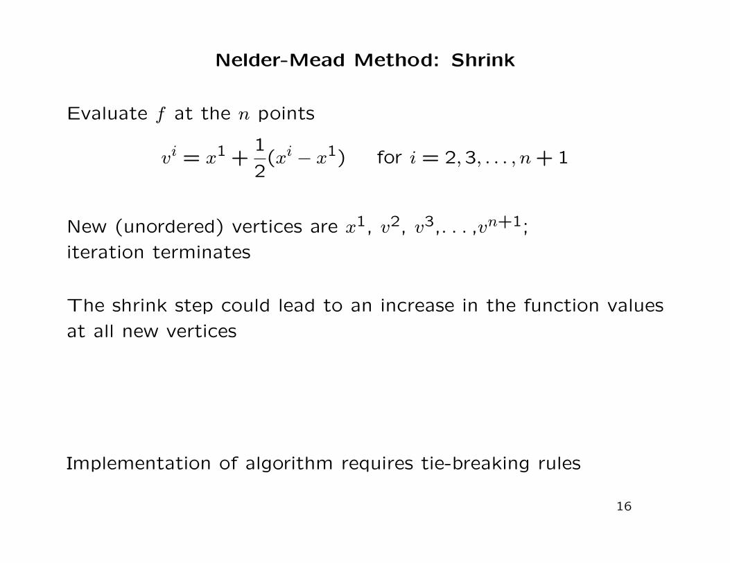
Nelder-Mead Method: Shrink

Evaluate f at the n points

vi = x1 +1

2(xi − x1) for i = 2,3, . . . , n+1

New (unordered) vertices are x1, v2, v3,. . . ,vn+1;

iteration terminates

The shrink step could lead to an increase in the function values

at all new vertices

Implementation of algorithm requires tie-breaking rules

16

Some Properties

Number of function evaluations depends on terminating step,

termination with reflect: 1; expand: 2; contract: 2; shrink: n+2

Except for a shrink step, the single new vertex always lies on the

line joining m and xn+1

Only very weak convergence results

17

Comment in a Paper on Convergence Analysis of the Method

Lagarias et al. (SIOPT, 1999):

At present there is no function in any dimension greater

than 1 for which the original Nelder-Mead algorithm has

been proved to converge to a minimizer.

Given all the known inefficiencies and failures of the Nelder-

Mead algorithm [...], one might wonder why it is used at

all, let alone why it is so extraordinarily popular.

18

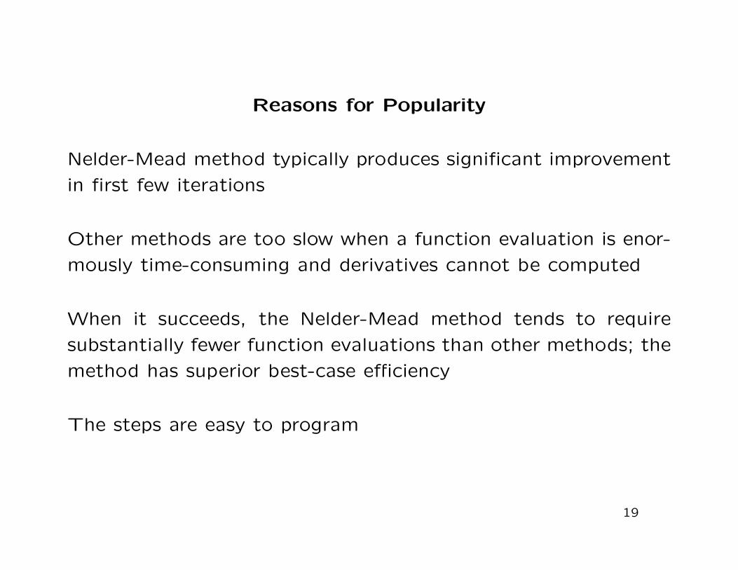
Reasons for Popularity

Nelder-Mead method typically produces significant improvement

in first few iterations

Other methods are too slow when a function evaluation is enor-

mously time-consuming and derivatives cannot be computed

When it succeeds, the Nelder-Mead method tends to require

substantially fewer function evaluations than other methods; the

method has superior best-case efficiency

The steps are easy to program

19

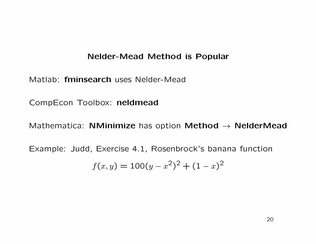
Nelder-Mead Method is Popular

Matlab: fminsearch uses Nelder-Mead

CompEcon Toolbox: neldmead

Mathematica: NMinimize has option Method → NelderMead

Example: Judd, Exercise 4.1, Rosenbrock’s banana function

f(x, y) = 100(y − x2)2 + (1− x)2

20

Derivative-free Methods and Derivatives

Finally, we want to make a strong statement that often

councils against the use of derivative-free methods: if you

can obtain clean derivatives (even if it requires consider-

able effort) and the functions defining your problem are

smooth and free of noise you should not use derivative-

free methods.

Introduction to derivative-free optimization

Conn/Scheinberg/Vicente (2009)

21

Optimality Conditions for Unconstrained Optimization

First-order necessary conditions

If f is continuously differentiable and x∗ is a local minimizer of

f , then ∇f(x∗) = 0.

Second-order necessary conditions

If f is twice continuously differentiable and x∗ is a local minimizer

of f , then ∇f(x∗) = 0 and Hf(x∗) is positive semi-definite, that

is, s⊤Hf(x∗)s ≥ 0 for all s ∈ Rn.

Second-order sufficient conditions

If f is twice continuously differentiable and at x∗ it holds that

∇f(x∗) = 0 and Hf(x∗) is positive definite, that is, s⊤Hf(x

∗)s > 0

for all s ∈ Rn, s ̸= 0, then x∗ is an isolated local minimizer of f .

22

Sufficient Condition for Global Optimality

If f is convex on Rn, then any local minimizer x∗ is a global

minimizer of f .

If f is convex and differentiable on Rn, then any point x∗ is a

global minimizer of f if and only if it is a stationary point, that

is, ∇f(x∗) = 0.

23

Newton’s Method

Quadratic approximation q of the function f (Taylor’s Theorem)

q(s) = f(x(k)) +∇f(x(k))⊤s+1

2s⊤Hf(x

(k))s

Necessary first-order condition ∇q(s) = 0 yields the Newton step

s(k) = −Hf(x(k))−1∇f(x(k))

Sufficient second-order condition:

Hq(s) = Hf(x(k)) is positive definite

Then s(k) is an isolated (global) minimizer of q

Iteration

x(k+1) = x(k) + s(k) = x(k) −Hf(x(k))−1∇f(x(k))

24

Newton’s Method

Initialization: Choose initial guess x(0) and stopping criteria ϵ, δ.

Iteration step: Compute ∇f(x(k)) and Hf(x(k)). Compute the

step s(k) as the solution to the system of linear equations

H(x(k))s(k) = −∇f(x(k)).

Set x(k+1) = x(k) + s(k).

Stopping rule: If ||x(k+1)−x(k)|| < ϵ(1+||x(k)||) and ||∇f(x(k))|| <δ(1 + |f(x(k))|), stop and report success.

25

Local Convergence Properties of Newton’s Method

Suppose that f is twice differentiable and that the Hessian Hf(x)is Lipschitz continuous in a neighborhood of a solution x∗ atwhich the second-order sufficient conditions are satisfied. Con-sider the Newton iteration

x(k+1) = x(k) + s(k)

Then,

(i) if the starting point x(0) is sufficiently close to x∗, then thesequence of iterates {x(k)} converges to x∗;

(ii) the rate of convergence is quadratic;

(iii) the sequence of gradient norms {||∇f(x(k))||} converges quadrat-ically to zero.

26

Newton’s Method

Mathematica: FindMinimum has option Method → Newton

Examples:

Exercise 4.1, Rosenbrock’s banana function

f(x, y) = 100(y − x2)2 + (1− x)2

Palgrave article, Example 4

f(x, y) = −(√

x1 +2√x2 +3

√(1− x1 − x2)

)Palgrave article, Example 2

f(x) = x(x− 2)2

27

Newton’s Method

Table 4.1: Consumers maximize utility

U(Y, Z) = u(Y, Z) = (Y α + Zα)ηα +M

subject to the budget constraint pY Y +pZZ+M = I. The FOCsare

pY = uY (Y, Z),

pZ = uZ(Y, Z).

The monopolist maximizes profits

Π(Y, Z) = (uY (Y, Z)− cY )Y + (uZ(Y, Z)− cZ)Z.

To avoid fractional powers of negative numbers define y = lnYand z = lnZ and solve the equivalent problem

maxy,z

π(y, z) = Π(ey, ez).

Take α = 0.98, η = 0.85, cY = 0.62, and cZ = 0.6.

28

Line Search Methods

Iteration k +1 of a line search method starting from x(k),

x(k+1) = x(k) + αks(k)

Search direction s(k), step length αk

Search direction s(k) should be a descent direction,

∇f(x(k))⊤s(k) < 0

Always possible to find unless ∇f(x(k)) = 0

From Taylor’s Theorem for sufficiently small ε > 0,

f(x(k) + εs(k)) = f(x(k)) + ε∇f(x(k))⊤s(k) + o(ε2) < f(x(k))

Function f decreases in the downhill direction s(k)

Suitable step length αk?

29

Line Search Methods

Computation of αk is the line search

Clearly we want to require

f(x(k) + αks(k)) < f(x(k))

Despite this requirement method may converge to a non-stationary

point ∇f(x(k)) ̸= 0 where descent directions still exist

Problem: decrease in f(x(k)) per iteration tends to zero

Line search steps are either too long or too short relative to

amount of decrease possible with a well-chosen step (pictures!)

30

Choosing a Step Length

Exact line search: find the optimal value for αk by solving the

one-dimensional optimization problem

minα

f(x(k) + αs(k))

Too expensive to find this global optimum for many iterations,

also unnecessary for convergence

Practical approaches perform inexact line search

Pick a step length that leads to a sufficient decrease in the

objective function value

31

Sufficient Decrease

Step length αk must satisfy Armijo condition

f(x(k) + αks(k)) ≤ f(x(k)) + αkβ∇f(x(k))⊤s(k)

for some β ∈ (0,1)

Right-hand-side f(x(k))+αβ∇f(x(k))⊤s(k) is linear function in α

(picture!)

Since ∇f(x(k))⊤s(k) < 0, the longer the step, the larger the

required decrease in f(x); thus, long steps with tiny decrease are

not permitted

32

Backtracking Armijo Line Search

Choose β ∈ (0,1), τ ∈ (0,1) and α(0) > 0 (e.g. α(0) = 1)

Set l = 0

Until f(x(k) + α(l)s(k)) ≤ f(x(k)) + α(l)β∇f(x(k))⊤s(k)

set α(l+1) = τα(l), increase l by 1

Set αk = α(l)

Iteration will stop after finitely many steps with positive αk

bounded away from zero

33

Backtracking Armijo Line Search

Theorem. Suppose that f ∈ C1, that ∇f is Lipschitz contin-uous with Lipschitz constant γ, that β ∈ (0,1) and that s(k) isa descent direction at x(k). Then the step length generated bythe backtracking Armijo line search satisfies

αk ≥ min

α(0),2τ(β − 1)∇f(x(k))⊤s(k)

γ||s(k)||2

,

where || · || is the Euclidean vector norm. 2

Lower bound on step length, so tiny steps are ruled out

Lower bound will only be small if ∇f(x(k))⊤s(k)

||s(k)||2is small

Problems arise if ∇f(x(k))⊤ and s(k) tend to becoming orthogonal

Choose appropriate descent direction

34

Method of Steepest Descent

Most intuitive choice for descent direction

s(k) = −∇f(x(k))

Greatest possible decrease in the linear approximation

f(x(k)) +∇f(x(k))⊤s(k)

(for a step s(k) of fixed norm)

Called the steepest descent direction

Line search with the steepest descent direction has very nice

theoretical properties

35

Global Convergence of the Steepest Descent Method

Theorem. Suppose that f is continuously differentiable and

that ∇f is Lipschitz continuous on Rn. Then for the sequence

{x(k)} of iterates generated by a line search method using the

steepest descent direction and the backtracking Armijo line search

one of the following three conditions must hold.

(C1) ∇f(x(k)) = 0 for some k ≥ 0.

(C2) limk→∞∇f(x(k)) = 0.

(C3) limk→∞ f(x(k)) = −∞.

2

Steepest descent method has the global convergence property.

36

Poor Performance in Practice

Rate of convergence is linear

In practice convergence is usually very slow

Numerical convergence sometimes does not occur at all as the

iteration stagnates

Method is considered useless in practice

Palgrave article, Example 3

37

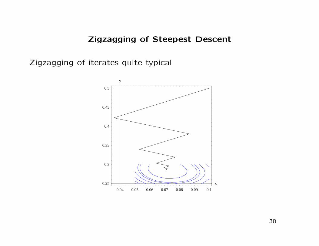
Zigzagging of Steepest Descent

Zigzagging of iterates quite typical

0.04 0.05 0.06 0.07 0.08 0.09 0.1

0.25

0.3

0.35

0.4

0.45

0.5

x

y

38

Line Search with Newton Direction

Newton direction: s(k) = −Hf(x(k))−1∇f(x(k))

Theorem. Suppose that f is twice continuously differentiableand that ∇f is Lipschitz continuous on Rn. If for the sequence{x(k)} of iterates generated by a line search method using theNewton direction and the backtracking Armijo line search theHessian matrices Hf(x

(k)) are positive definite with eigenvaluesthat are uniformly bounded away from zero, then one of theconditions (C1), (C2), (C3) must hold:

(C1) ∇f(x(k)) = 0 for some k ≥ 0.

(C2) limk→∞∇f(x(k)) = 0.

(C3) limk→∞ f(x(k)) = −∞.

2

Problem again: strong assumptions on Hessian matrix Hf(x)

39

Line Search Newton with Hessian Modification

Away from local minimizer, the Hessian matrix Hf(x) may notbe positive definite, and so Newton direction s(k) defined byHf(x

(k))s(k) = ∇f(x(k)) may not be a descent direction

Approach to overcome this difficulty: modify Hessian matrix

Add a matrix M(x(k)) to the Hessian so that M(x(k)) +H(x(k))is “sufficiently” positive definite

Then the direction s(k) is determined by the solution to(M(x(k)) +H(x(k))

)s(k) = ∇f(x(k))

Whenever H(x(k)) is sufficiently positive definite by itself, thenM(x(k)) = 0

Convergence results for properly chosen modifications are similarto those for the case of positive definite Hessian matrix

40

Computation of Second Derivatives

Most tedious step in Newton’s method: computation of Hessianmatrix H(x(k))

Recent development of automatic differentiation techniquesmakes it possible to apply Newton’s method without requiringthe user to supply second derivatives

If automatic differentiation is impossible or too costly, then otherapproaches are needed

Estimating second derivatives by finite differences of first deriva-tives

(Hf(x))·j =∇f(x+ hej)−∇f(x)

h

where ej is the ith unit vector

Difficulty: choosing appropriate value for scalar h > 0

41

Quasi-Newton Methods

Quasi-Newton methods use suitable approximations Bk of the

Hessian Hf(xk)

Require only gradient of the objective function (like steepest

descent)

Measure changes in the gradient to obtain information on the

curvature of f and to update an approximation Bk of Hf(xk)

42

Positive Definite Approximation of Hessian

Quadratic approximation q of the function f (Taylor’s Theorem)

q(s) = f(x(k)) +∇f(x(k))⊤s+1

2s⊤Hf(x

(k))s

Replace Hessian Hf(x(k)) by symmetric positive definite Bk

qk(s) = f(x(k)) +∇f(x(k))⊤s+1

2s⊤Bks

Note that

qk(0) = f(x(k)) and ∇qk(0) = ∇f(x(k))

qk is convex and quadratic and so

s(k) = −(Bk)−1∇f(x(k))

is the global minimizer

New iterate determined with backtracking Armijo line search

x(k+1) = x(k) + αks(k)

43

Requirements on the Approximate Hessian

Iteration is Newton line search with approximate Hessian Bk in

place of true Hessian

New quadratic model

qk+1(s) = f(x(k+1)) +∇f(x(k+1))⊤s+1

2s⊤Bk+1s

Requirements on Bk+1?

Gradient of qk+1 should match gradient of f at the last two

iterates

∇qk+1(0) = ∇f(x(k+1)) and ∇qk+1(−αks(k)) = ∇f(x(k))

First equations holds automatically

44

Secant Equation

Second condition

∇qk+1(−αks(k)) = ∇f(x(k+1))− αkBk+1s

(k) = ∇f(x(k))

is equivalent to

Bk+1αks(k) = ∇f(x(k+1))−∇f(x(k))

With zk = x(k+1)−x(k) and yk = ∇f(x(k+1))−∇f(x(k)) we obtainthe secant equation

Bk+1zk = yk

The symmetric positive definite matrix Bk+1 must map the changezk in the iterates into the change yk in the gradients at the iter-ates

Implications for search direction and change in gradients

z⊤k yk = z⊤k Bk+1zk > 0

Satisfied by iterates chosen by backtracking Armijo line search

45

Solutions to Secant Equation

Under the condition z⊤k yk > 0 there always exist solutions to the

secant equations

In fact, infinite number of solutions

Different additional requirements lead to different solutions Bk+1,

as a result there are numerous quasi-Newton methods

Most effective of all quasi-Newton updating formulas

BFGS updating formula (Broyden, Fletcher, Goldfarb, Shanno)

Bk+1 = Bk −Bkzk(Bkzk)

⊤

z⊤k Bkzk+

yky⊤k

y⊤k zk

If Bk is symmetric positive definite, then so is Bk+1

46

BFGS Method

Initial matrix B0: identity matrix, multiple thereof, or Hessian of

f at x(0)

BFGS method has superlinear convergence on many practical

problems

Global convergence property (under some technical conditions)

Even if sequence of iterates {x(k)} converges, the sequence of

matrices {Bk} may not converge to the true Hessian at the so-

lution

47

Trust-region Methods

Line search methods:

Pick a descent direction s(k) based on an approximation for f

Choose suitable step length αk to decrease f(x(k) + αks(k))

Trust-region methods:

Define a region around current iterate x(k) within which approx-

imation is trusted

Choose the step to be an approximate minimizer of the approxi-

mation for f ; that is, choose direction and length simultaneously

Reduce the size of the trust region if the step is not acceptable

48

Trust-region Subproblem

Once again we use a quadratic model of f ,

qk(s) = f(x(k)) +∇f(x(k))⊤s+1

2s⊤Bks

Trust-region subproblem

mins∈Rn

qk(s) subject to ||s|| ≤ ∆k

with trust-region radius ∆k > 0

Use Euclidean norm, so {s : ||s|| ≤ ∆k} is the ball of radius ∆k

Constraint can be written as s⊤s ≤ ∆2k

Unlike for line search methods, Bk = Hf(x(k)) is always permitted

49

A Key Ingredient of the Trust-region Algorithm

Evaluation of a possible step s(k) from x(k) to x(k+1) = x(k)+s(k)

Predicted reduction by quadratic model: qk(0)− qk(s(k))

Actual reduction in function values: f(x(k))− f(x(k) + s(k))

Fraction of predicted reduction that is realized by the actualreduction

ρk =f(x(k))− f(x(k) + s(k))

qk(0)− qk(s(k))

If ratio ρk is close to (or larger than) 1, then there appears tobe good agreement between f and qk, so trust-region radius willbe increased

If ρk is close to zero or even negative, then we set x(k+1) = x(k)

and reduce the trust region radius

50

Basic Trust-region Algorithm

Parameters 0 < ηs < ηv < 1, γi ≥ 1, 0 < γd < 1

Given x(k), ∆k > 0, iteration k +1:

Approximately solve the trust-region subproblem to find s(k) forwhich qk(s

(k)) < qk(0) = f(x(k)) and ||s(k)|| < ∆k and define

ρk =f(x(k))− f(x(k) + s(k))

f(x(k))− qk(s(k))

If ρk ≥ ηv [very successful],

set x(k+1) = x(k) + s(k) and ∆k+1 = γi∆k

Otherwise, if ρk ≥ ηs [successful],

set x(k+1) = x(k) + s(k) and ∆k+1 = ∆k

Otherwise [unsuccessful],

set x(k+1) = x(k) and ∆k+1 = γd∆k

51

Practical Considerations

Popular values: ηv ∈ {0.9,0.99}, ηs ∈ {0.1,0.01}, γi = 2, γd = 0.5

Parameter values may be allowed to vary from iteration to iter-

ation

Trust-region radius is not increased for very successful iterations

if ||s(k)|| is much smaller ∆k

Open problems:

Solving the trust-region subproblem

Finding conditions for convergence

52

Sufficient reduction

Line search methods do not require step length to be chosen

optimally to be globally convergent

Similarly, unnecessary and computationally inefficient to solve

trust-region subproblem exactly

Sufficient reduction in approximation qk(s) suffices

Reduction in the approximation should be at least as large as

from an iteration of steepest descent

53

Cauchy Point

The solution to

minα∈R

qk(−α∇f(x(k))) subject to ∥ − α∇f(x(k))∥ ≤ ∆k

yields the Cauchy point

sCk = −τk∆k∇f(x(k))

∥∇f(x(k))∥where constant τk ∈ (0,1] depends on the curvature of qk andtrust-region radius ∆k

Closed-form solution for τk exists, Cauchy point is inexpensiveto calculate

The approximate solution s(k) of the trust region subproblemmust now satisfy

qk(s(k)) ≤ qk(s

Ck ) and ||s(k)|| ≤ ∆k

54

Improvement by the Cauchy Point

The reduction in the quadratic approximation qk can be related

to ∥∇f(x(k))∥, which is a measure from distance to optimality.

Theorem. Let qk be the second-order approximation of the

objective function f at x(k) and let sCk be its Cauchy point in the

trust region defined by ∥s∥ ≤ ∆k. Then

qk(0)− qk(sCk ) = f(x(k))− qk(s

Ck )

≥1

2∥∇f(x(k))∥min

∥∇f(x(k))∥1+ ∥B(x(k))∥

,∆k

.

2

The theorem establishes a lower bound on the improvement in

qk if trust region radius ∆k is bounded away from zero.

55

Global Convergence

Theorem. Consider the sequence {x(k)} of iterates generated

by a trust region method whose steps do at least as well as the

Cauchy point. Suppose that f is twice continuously differentiable

and both the Hessian of f and of the quadratic approximation qkare bounded for all k. Then one of the conditions (C1), (C2),

(C3) must hold:

(C1) ∇f(x(k)) = 0 for some k ≥ 0.

(C2) limk→∞∇f(x(k)) = 0.

(C3) limk→∞ f(x(k)) = −∞.

2

56

Improvements on the Cauchy Point

Assume matrix B in second-order approximation qk is positive

definite

Dogleg method makes two steps:

First step in the steepest descent direction

Second step in the modified Newton direction

Two-dimensional subspace minimization:

Single step that must lie in the span of the two directions used

by the dogleg method

Additional solution approaches for the trust-region subproblem

exist

57

Computer Implementation

Matlab: fminunc is a solver for nonlinear unconstrained opti-

mzation

Uses a trust-region method with subspace minimization as de-

fault

Has an option for BFGS Quasi-Newton method with a line search

procedure

58