1 optimization introduction & 1-d unconstrained optimization
TRANSCRIPT

1
Optimization
Introduction&
1-D Unconstrained Optimization
2
Mathematical Background
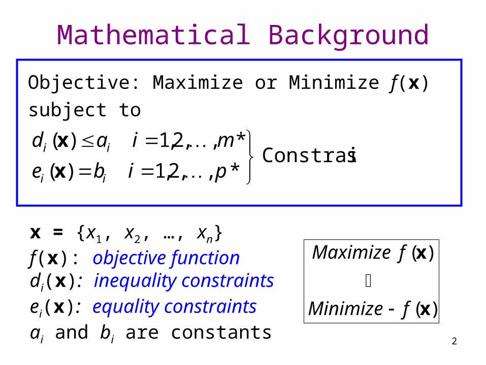
Objective: Maximize or Minimize f(x)
subject to
sConstraint*,,2,1)(
*,,2,1)(
pibe
miad
ii
ii
x
x
x = {x1, x2, …, xn} f(x): objective functiondi(x): inequality constraintsei(x): equality constraintsai and bi are constants
)(
)(
x
x
fMinimize
fMaximize
3
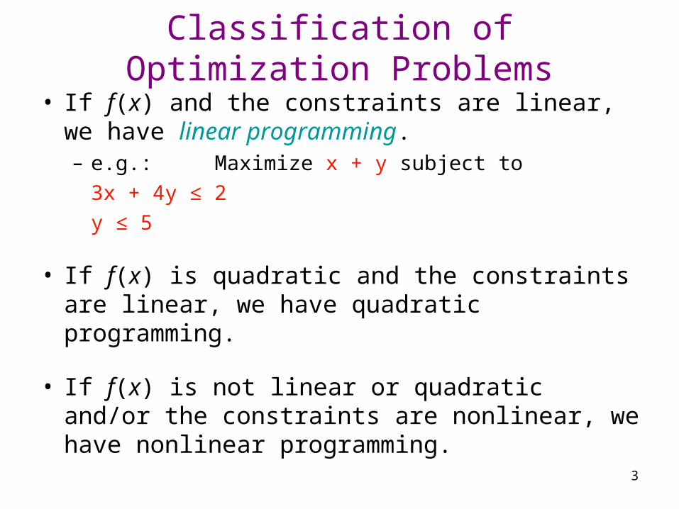
• If f(x) and the constraints are linear, we have linear programming.– e.g.: Maximize x + y subject to
3x + 4y ≤ 2
y ≤ 5
• If f(x) is quadratic and the constraints are linear, we have quadratic programming.
• If f(x) is not linear or quadratic and/or the constraints are nonlinear, we have nonlinear programming.
Classification of Optimization Problems
4
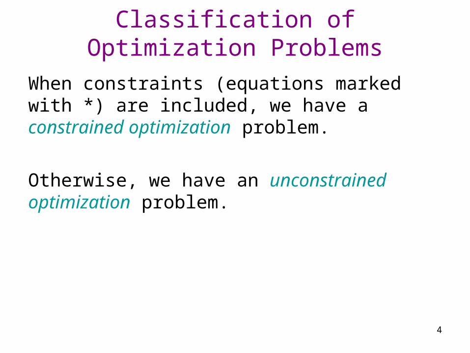
When constraints (equations marked with *) are included, we have a constrained optimization problem.
Otherwise, we have an unconstrained optimization problem.
Classification of Optimization Problems
5
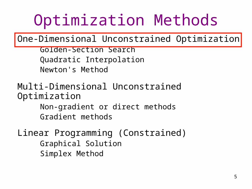
Optimization MethodsOne-Dimensional Unconstrained Optimization
Golden-Section SearchQuadratic InterpolationNewton's Method
Multi-Dimensional Unconstrained OptimizationNon-gradient or direct methodsGradient methods
Linear Programming (Constrained)Graphical SolutionSimplex Method
6
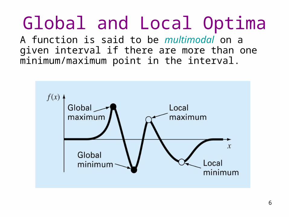
A function is said to be multimodal on a given interval if there are more than one minimum/maximum point in the interval.
Global and Local Optima
7
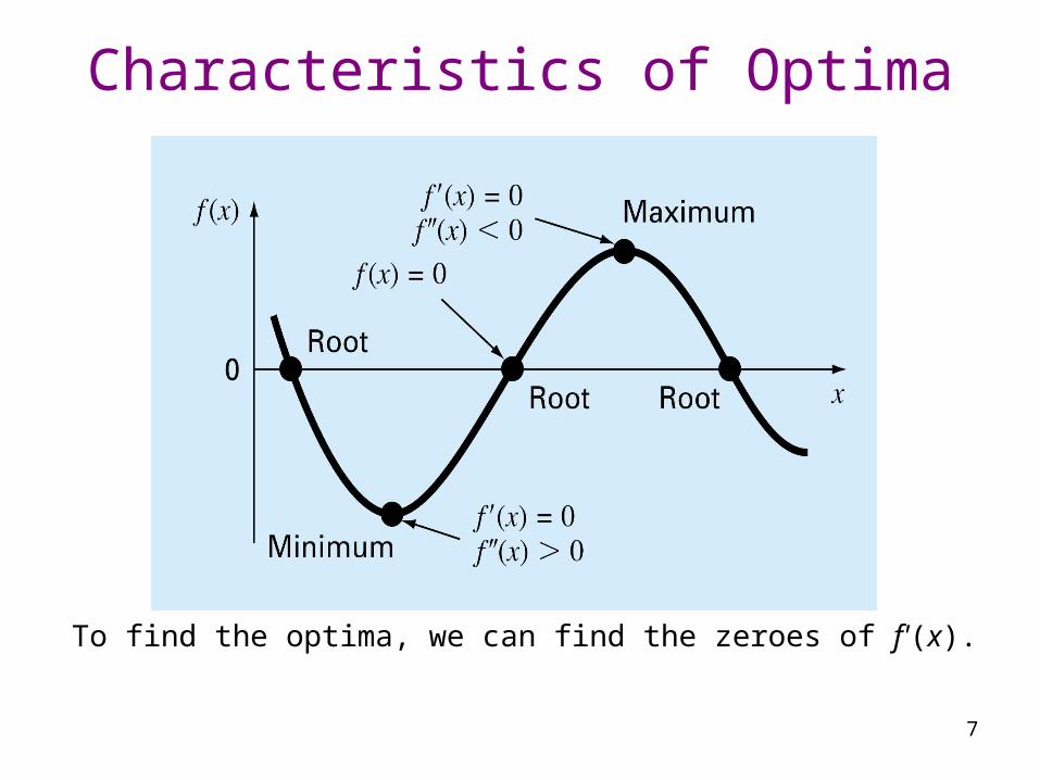
Characteristics of Optima
To find the optima, we can find the zeroes of f'(x).
8
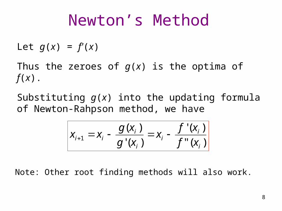
Newton’s Method
Let g(x) = f'(x)
Thus the zeroes of g(x) is the optima of f(x).
Substituting g(x) into the updating formula of Newton-Rahpson method, we have
)("
)('
)('
)(1
i
ii
i
iii xf
xfx
xg
xgxx
Note: Other root finding methods will also work.
9
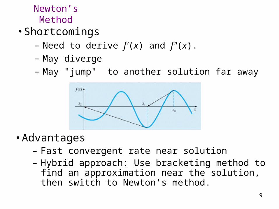
Newton’s Method
• Shortcomings– Need to derive f'(x) and f"(x).– May diverge– May "jump" to another solution far away
• Advantages– Fast convergent rate near solution– Hybrid approach: Use bracketing method to find an
approximation near the solution, then switch to Newton's method.
10
xxll x xuu x x
ff((xx))
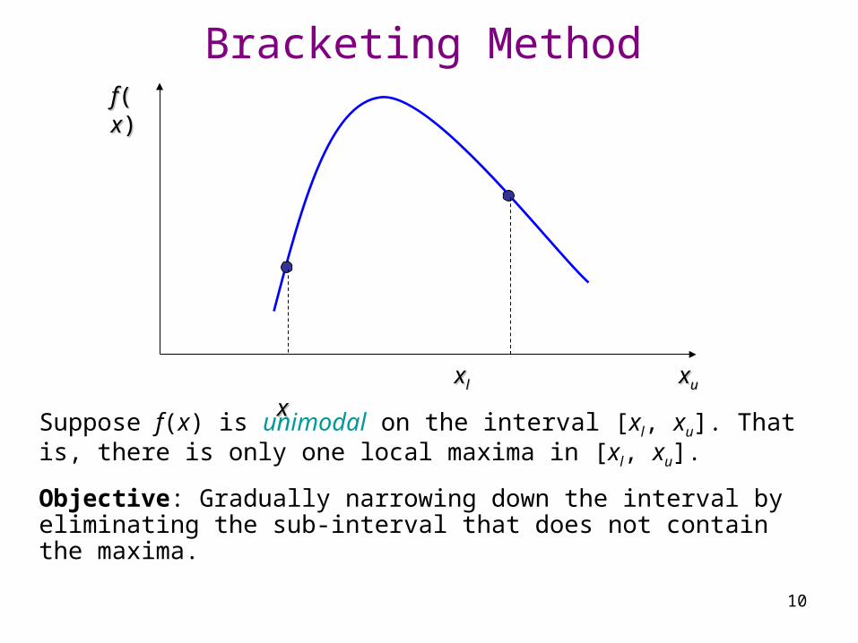
Bracketing Method
Suppose f(x) is unimodal on the interval [xl, xu]. That is, there is only one local maxima in [xl, xu].
Objective: Gradually narrowing down the interval by eliminating the sub-interval that does not contain the maxima.
11
xxll x xaa x xbb x xuu x x
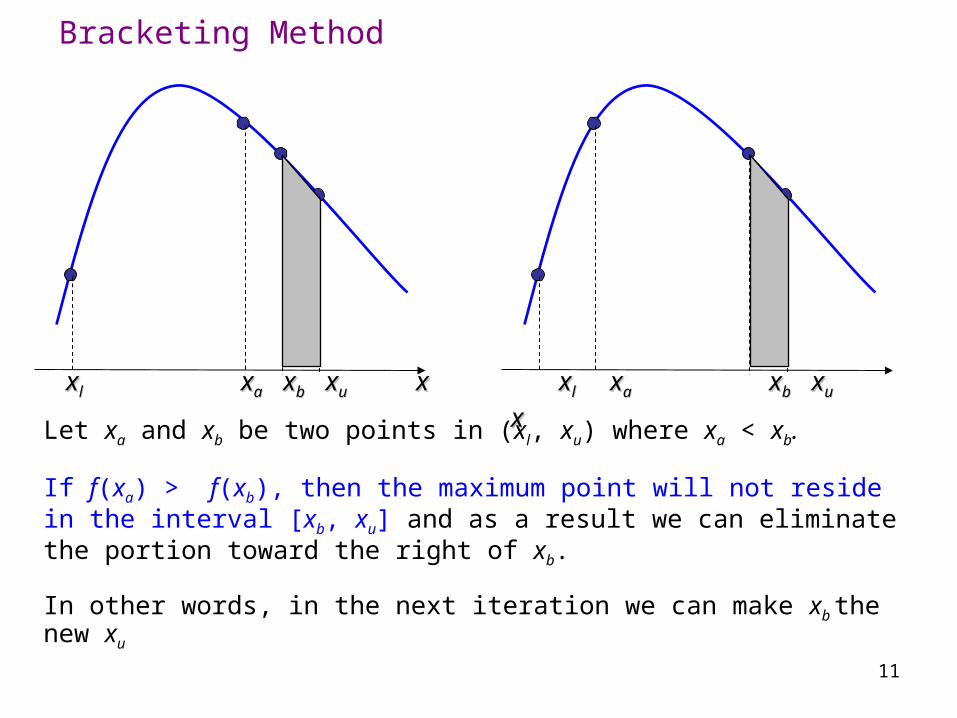
Bracketing Method
Let xa and xb be two points in (xl, xu) where xa < xb.
If f(xa) > f(xb), then the maximum point will not reside in the interval [xb, xu] and as a result we can eliminate the portion toward the right of xb.
In other words, in the next iteration we can make xb the new xu
xxll x xaa x xbb x xuu x x
12
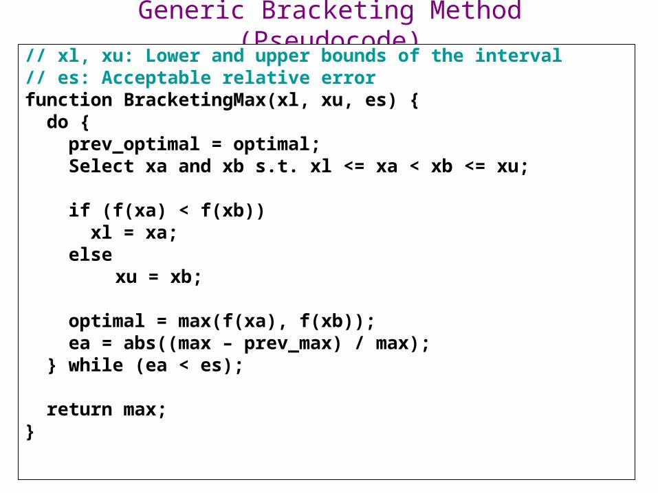
Generic Bracketing Method (Pseudocode)// xl, xu: Lower and upper bounds of the interval// es: Acceptable relative errorfunction BracketingMax(xl, xu, es) { do { prev_optimal = optimal; Select xa and xb s.t. xl <= xa < xb <= xu;
if (f(xa) < f(xb)) xl = xa; else
xu = xb;
optimal = max(f(xa), f(xb)); ea = abs((max – prev_max) / max); } while (ea < es);
return max;}
13
How would you suggest we select xa and xb (with the objective to minimize computation)?
– Eliminate as much interval as possible in each iteration
• Set xa and xb close to the center so that we can halve the interval in each iteration
• Drawbacks: function evaluation is usually a costly operation.
– Minimize the number of function evaluations
• Select xa and xb such that one of them can be reused in the next iteration (so that we only need to evaluate f(x) once in each iteration).
• How should we select such points?
Bracketing Method
14
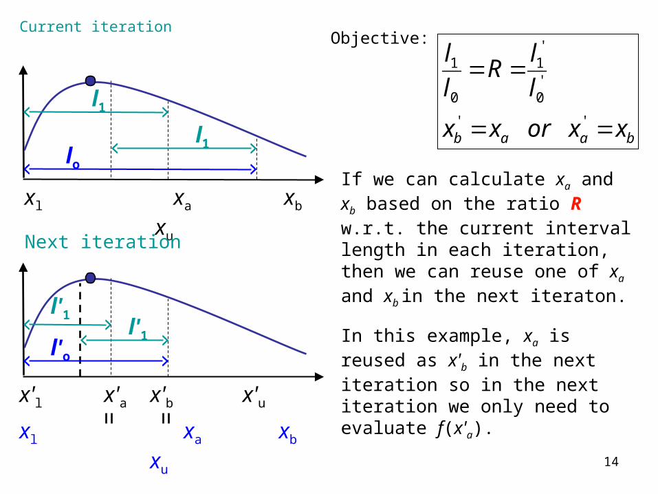
xl xa xb xu
Current iteration
Next iteration
x'l x'a x'b x'u
If we can calculate xa and xb based on the ratio R w.r.t. the current interval length in each iteration, then we can reuse one of xa and xb in the next iteraton.
In this example, xa is reused as x'b in the next iteration so in the next iteration we only need to evaluate f(x'a).
l1
l1
lo
l'1l'1
l'o
baab xxorxx
l
lR
l
l
''
'0
'1
0
1Objective:
xl xa xb xu
15
xl xa xb xu
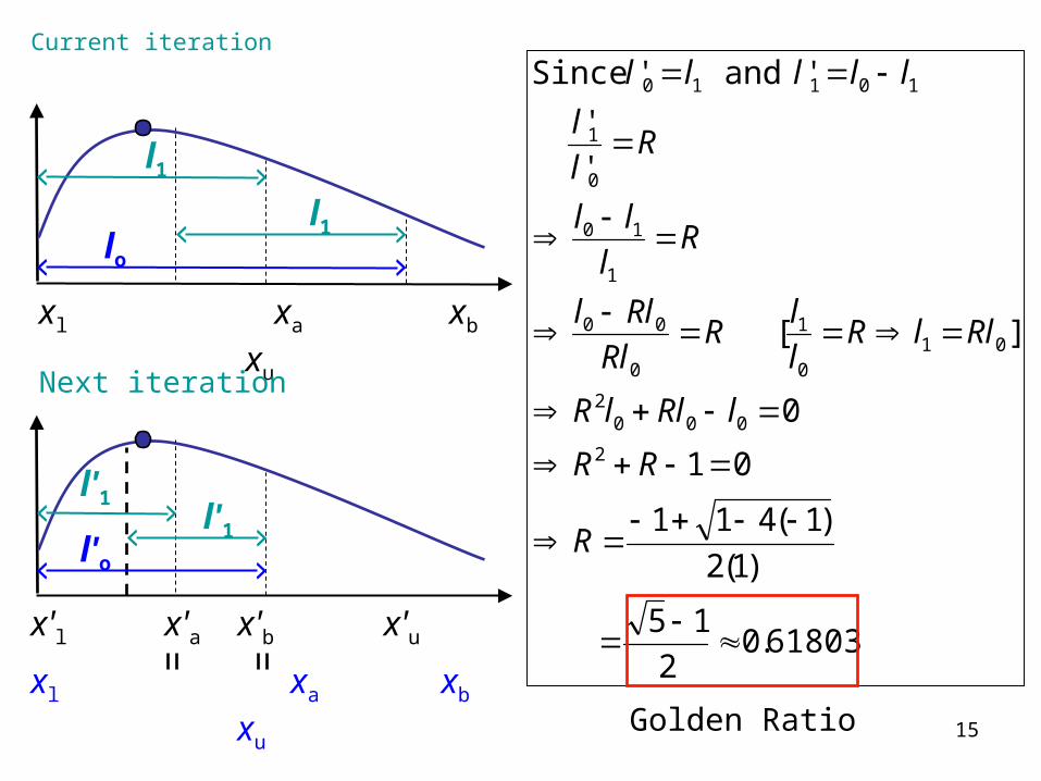
Current iteration
Next iteration
x'l x'a x'b x'u
l1
l1
lo
l'1l'1
l'o
61803.02
15
)1(2
)1(411
01
0
][
'
'
'and'Since
2
0002
010
1
0
00
1
10
0
1
10110
R
RR
lRllR
RllRl
lR
Rl
Rll
Rl
ll
Rl
l
lllll
Golden Ratioxl xa xb xu
16
)(2
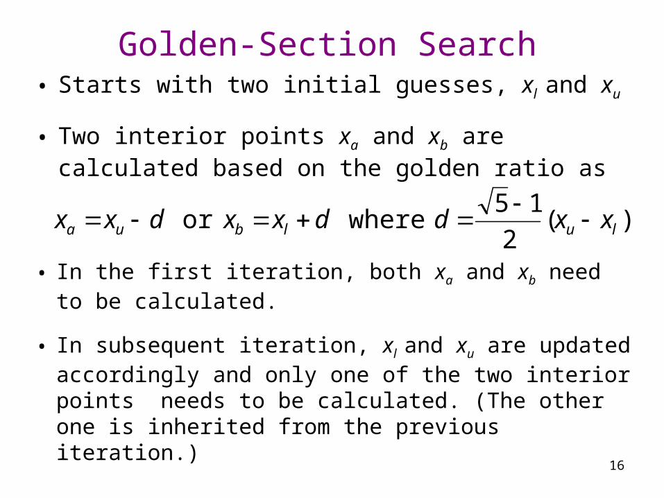
15whereor lulbua xxddxxdxx
• Starts with two initial guesses, xl and xu
• Two interior points xa and xb are calculated based on the golden ratio as
Golden-Section Search
• In the first iteration, both xa and xb need to be calculated.
• In subsequent iteration, xl and xu are updated accordingly and only one of the two interior points needs to be calculated. (The other one is inherited from the previous iteration.)
17
• In each iteration the interval is reduced to about 61.8% (Golden ratio) of its previous length.
• After 10 iterations, the interval is shrunk to about (0.618)10 or 0.8% of its initial length.
• After 20 iterations, the interval is shrunk to about (0.618)20 or 0.0066%.
Golden-Section Search
18
x0 x1 x3 x2 x
f(x)
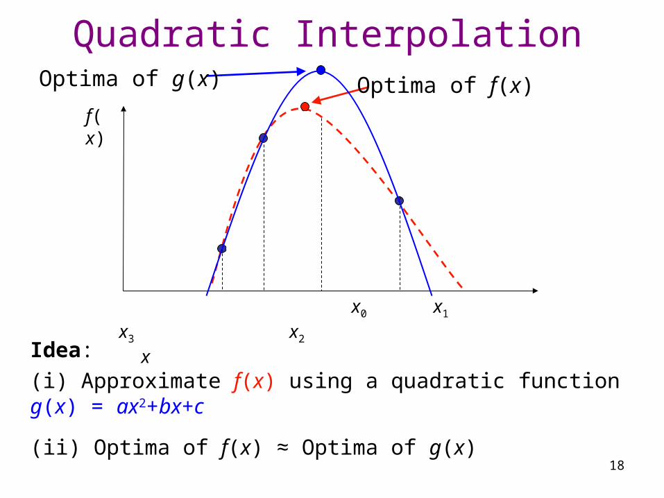
Quadratic Interpolation
Idea:
(i) Approximate f(x) using a quadratic function g(x) = ax2+bx+c
(ii) Optima of f(x) ≈ Optima of g(x)
Optima of f(x)Optima of g(x)
19
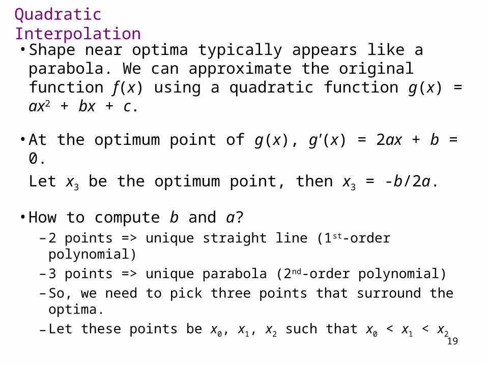
• Shape near optima typically appears like a parabola. We can approximate the original function f(x) using a quadratic function g(x) = ax2 + bx + c.
• At the optimum point of g(x), g'(x) = 2ax + b = 0.
Let x3 be the optimum point, then x3 = -b/2a.
• How to compute b and a?– 2 points => unique straight line (1st-order polynomial) – 3 points => unique parabola (2nd-order polynomial)– So, we need to pick three points that surround the
optima.
– Let these points be x0, x1, x2 such that x0 < x1 < x2
Quadratic Interpolation
20
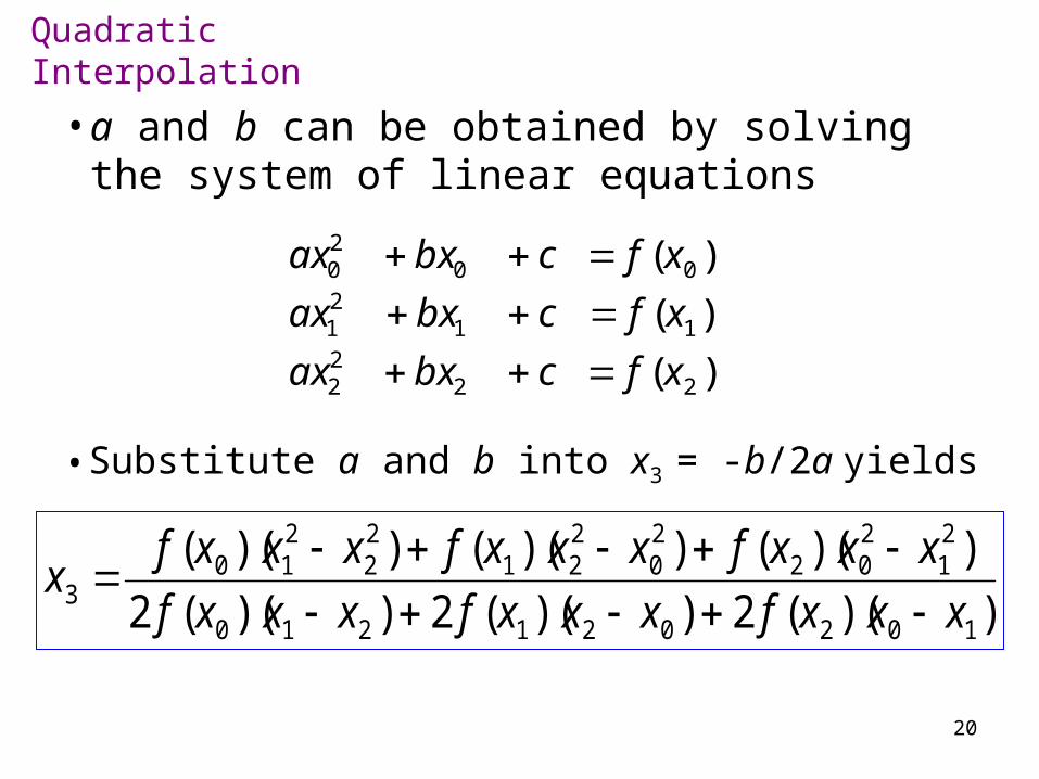
• a and b can be obtained by solving the system of linear equations
)(
)(
)(
2
1
0
222
121
020
xf
xf
xf
cbxax
cbxax
cbxax
))((2))((2))((2
))(())(())((
102021210
21
202
20
221
22
210
3 xxxfxxxfxxxf
xxxfxxxfxxxfx
• Substitute a and b into x3 = -b/2a yields
Quadratic Interpolation
21
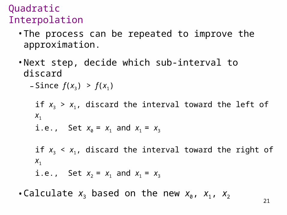
• The process can be repeated to improve the approximation.
• Next step, decide which sub-interval to discard– Since f(x3) > f(x1)
if x3 > x1, discard the interval toward the left of x1
i.e., Set x0 = x1 and x1 = x3
if x3 < x1, discard the interval toward the right of x1
i.e., Set x2 = x1 and x1 = x3
• Calculate x3 based on the new x0, x1, x2
Quadratic Interpolation
22
Summary
• Basics– Minimize f(x) = Maximize -f(x)
– If f'(x) exists, then to find the optima of f(x), we can find the zero of f'(x).
• Beware of inflection points of f(x)
• Bracketing methods– Golden-Section Search and Quadratic Interpolation– How to select points and discard intervals