bayesian decision theory - computer sciencerlaz/prec20092/slides/bayesiandecisiontheory.pdf ·...

Bayesian Decision Theory

Prof. Richard Zanibbi

Bayesian Decision Theory

The Basic Idea

To minimize errors, choose the least risky class, i.e. the class for which the expected loss is smallest

Assumptions

Problem posed in probabilistic terms, and all relevant probabilities are known

2

Probability Mass vs. Probability Density Functions

Probability Mass Function, P(x)

Probability for values of discrete random variable x. Each value has its own associated probability

Probability Density, p(x)

Probability for values of continuous random variable x. Probability returned is for an interval within which the value lies (intervals defined by some unit distance)

3

! = {v1, . . . , vm}

P (x) ! 0, and!

x"!

P (x) = 1

Pr[x " (a, b)] =

" b

ap(x) dx

p(x) ! 0 and

" #

$#p(x) dx = 1

1

! = {v1, . . . , vm}

P (x) ! 0, and!

x"!

P (x) = 1

Pr[x " (a, b)] =

" b

ap(x) dx

p(x) ! 0 and

" #

$#p(x) dx = 1

1

Prior ProbabilityDefinition ( P( w ) )

The likelihood of a value for a random variable representing the state of nature (true class for the current input), in the absence of other information

• Informally, “what percentage of the time state X occurs”

Example

The prior probability that an instance taken from two classes is provided as input, in the absence of any features (e.g. P(cat) = 0.3, P(dog) = 0.7)

4

Class-Conditional Probability Density Function (for Continuous Features)

Definition ( p( x | w ) )

The probability of a value for continuous random variable x, given a state of nature w

• For each value of x, we have a different class-conditional pdf for each class in w (example next slide)

5

Example: Class-Conditional Probability Densities

6

9 10 11 12 13 14 15

0.1

0.2

0.3

0.4

p(x|!i)

x

!1

!2

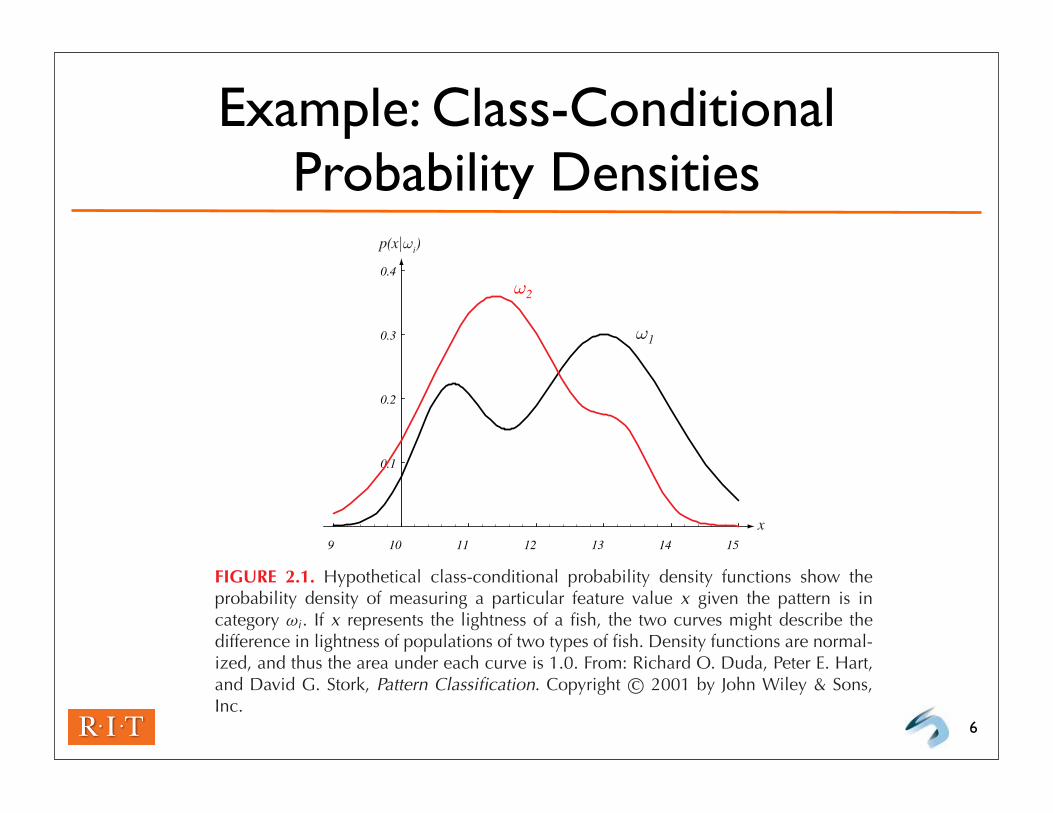
FIGURE 2.1. Hypothetical class-conditional probability density functions show theprobability density of measuring a particular feature value x given the pattern is incategory !i . If x represents the lightness of a fish, the two curves might describe thedifference in lightness of populations of two types of fish. Density functions are normal-ized, and thus the area under each curve is 1.0. From: Richard O. Duda, Peter E. Hart,and David G. Stork, Pattern Classification. Copyright c! 2001 by John Wiley & Sons,Inc.

Bayes Formula

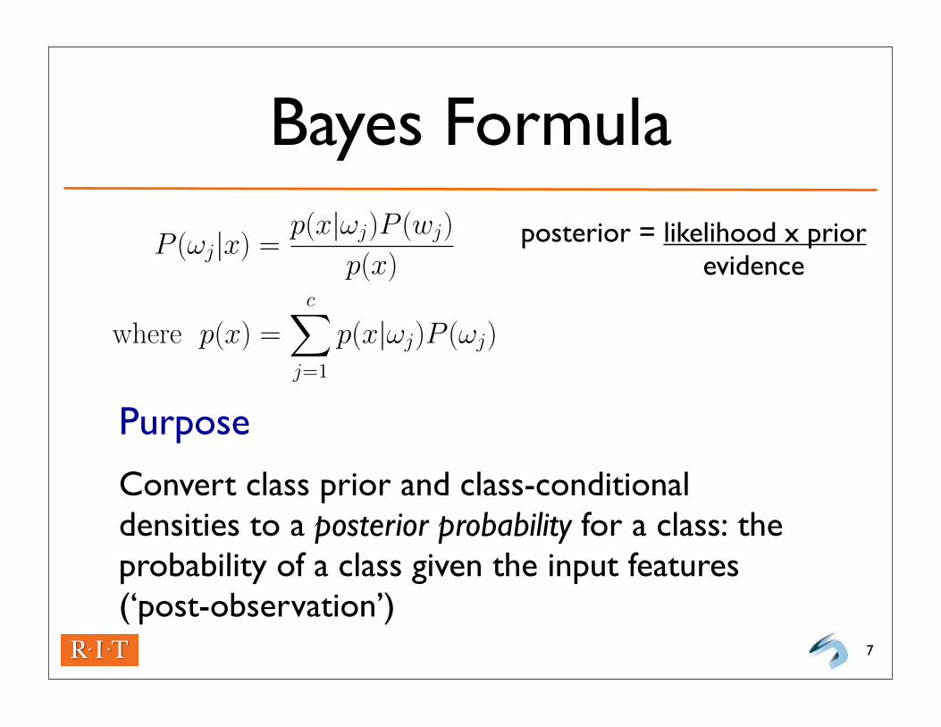
Purpose

Convert class prior and class-conditional densities to a posterior probability for a class: the probability of a class given the input features (‘post-observation’)

7

posterior = likelihood x prior evidence

P (!j|x) =p(x|!j)P (wj)

p(x)

where p(x) =c!

j=1

p(x|!j)P (!j)

2

Example: Posterior Probabilities

8

0.2

0.4

0.6

0.8

1

P(!i|x)

x

!1

!2

9 10 11 12 13 14 15

FIGURE 2.2. Posterior probabilities for the particular priors P(!1) = 2/3 and P(!2)

= 1/3 for the class-conditional probability densities shown in Fig. 2.1. Thus in thiscase, given that a pattern is measured to have feature value x = 14, the probability it isin category !2 is roughly 0.08, and that it is in !1 is 0.92. At every x, the posteriors sumto 1.0. From: Richard O. Duda, Peter E. Hart, and David G. Stork, Pattern Classification.Copyright c! 2001 by John Wiley & Sons, Inc.

Expected Loss or Conditional Risk of an Action

Explanation

The expected (“average”) loss for taking an action (choosing a class) given an input vector, for a given conditional loss function (lambda)

10

R(!i|x) =c!

j=1

"(!i|#j)P (#j|x)

1

Decision Functions and Overall Risk

Decision Function or Decision Rule

( alpha(x) ): takes on the value of exactly one action for each input vector x

Overall Risk

The expected (average) loss associated with a decision rule

11

R(!i|x) =c!

j=1

"(!i|#j)P (#j|x)

R =

"R(!(x)|x)p(x) dx

1

Bayes Decision Rule

Idea

Minimize the overall risk, by choosing the action with the least conditional risk for input vector x

Bayes Risk (R*)

The resulting overall risk produced using this procedure. This is the best performance that can be achieved given available information.

12

Bayes Decision Rule: Two Category Case

Bayes Decision Rule

For each input, select class with least conditional risk, i.e. choose class one if:

where

13

Bayesian Decision Rules

!ij = !("i|#j)

R("1|x) < R("2|x)

R(#1|x) = !11P (#1|x) + !12P (#2|x)

R(#2|x) = !21P (#1|x) + !22P (#2|x)

(!21 ! !11)P (#1|x) > (!12 ! !22)P (#2|x)

(!21 ! !11)p(x|#1)P (#1) > (!12 ! !22)p(x|#2)P (#2)

p(x|#1)

p(x|#2)>

!12 ! !22

!21 ! !11

P (#2)

P (#1)

1


!ij = !("i|#j)

R("1|x) < R("2|x)

R("1|x) = !11P (#1|x) + !12P (#2|x)

R("2|x) = !21P (#1|x) + !22P (#2|x)

(!21 ! !11)P (#1|x) > (!12 ! !22)P (#2|x)

(!21 ! !11)p(x|#1)P (#1) > (!12 ! !22)p(x|#2)P (#2)

p(x|#1)

p(x|#2)>

!12 ! !22

!21 ! !11

P (#2)

P (#1)

1


!ij = !("i|#j)

R("1|x) < R("2|x)

R("1|x) = !11P (#1|x) + !12P (#2|x)

R("2|x) = !21P (#1|x) + !22P (#2|x)

(!21 ! !11)P (#1|x) > (!12 ! !22)P (#2|x)

(!21 ! !11)p(x|#1)P (#1) > (!12 ! !22)p(x|#2)P (#2)

p(x|#1)

p(x|#2)>

!12 ! !22

!21 ! !11

P (#2)

P (#1)

1

Alternate Equivalent Expressions of Bayes Decision Rule (“Choose Class One If...”)

Posterior Class Probabilities

Class Priors and Conditional DensitiesProduced by applying Bayes Formula to the above, multiplying both sides by p(x)

Likelihood Ratio14


!ij = !("i|#j)

R("1|x) < R("2|x)

R("1|x) = !11P (#1|x) + !12P (#2|x)

R("2|x) = !21P (#1|x) + !22P (#2|x)

(!21 ! !11)P (#1|x) > (!12 ! !22)P (#2|x)

(!21 ! !11)p(x|#1)P (#1) > (!12 ! !22)p(x|#2)P (#2)

p(x|#1)

p(x|#2)>

!12 ! !22

!21 ! !11

P (#2)

P (#1)

1


!ij = !("i|#j)

R("1|x) < R("2|x)

R("1|x) = !11P (#1|x) + !12P (#2|x)

R("2|x) = !21P (#1|x) + !22P (#2|x)

(!21 ! !11)P (#1|x) > (!12 ! !22)P (#2|x)

(!21 ! !11)p(x|#1)P (#1) > (!12 ! !22)p(x|#2)P (#2)

p(x|#1)

p(x|#2)>

!12 ! !22

!21 ! !11

P (#2)

P (#1)

1


!ij = !("i|#j)

R("1|x) < R("2|x)

R("1|x) = !11P (#1|x) + !12P (#2|x)

R("2|x) = !21P (#1|x) + !22P (#2|x)

(!21 ! !11)P (#1|x) > (!12 ! !22)P (#2|x)

(!21 ! !11)p(x|#1)P (#1) > (!12 ! !22)p(x|#2)P (#2)

p(x|#1)

p(x|#2)>

!12 ! !22

!21 ! !11

P (#2)

P (#1)

1

Example: Likelihood Ratio

16

x

!a

p(x|!1)p(x|!2)

!b

R1R2 R1R2

FIGURE 2.3. The likelihood ratio p(x|!1)/p(x|!2) for the distributions shown inFig. 2.1. If we employ a zero-one or classification loss, our decision boundaries aredetermined by the threshold "a. If our loss function penalizes miscategorizing !2 as !1

patterns more than the converse, we get the larger threshold "b, and hence R1 becomessmaller. From: Richard O. Duda, Peter E. Hart, and David G. Stork, Pattern Classifica-tion. Copyright c! 2001 by John Wiley & Sons, Inc.

Discriminants for Two Categories

For Two Categories

We can use a single discriminant function, with decision rule: choose class one if the discriminant returns a value > 0.

Example: Zero-One Loss

19

3 two-category again

g(x) = P (!1|x)! P (!2|x)

g(x) = lnp(x|!1)

p(x|!2)+ ln

P (!1)

P (!2)

4 Gaussian (univariate normal)

P (x) =1"2"#

exp

!!1

2

"x! µ

#

#2$

µ =

% #

!#x p(x) dx

#2 =

% #

!#(x! µ)2p(x) dx

5 Multivariate normal density

p(x) =1

(2")d/2|!|1/2exp

&!1

2(x! µ)t!!1(x! µ)

'

µ =

% #

!#x p(x) dx

! =

%(x! µ)(x! µ)tp(x)dx

3

Example: Decision Regions for Binary Classifier

20

0

0.1

0.2

0.3

decisionboundary

p(x|!2)P(!2)

R1

R2

p(x|!1)P(!1)

R2

0

5

0

5

FIGURE 2.6. In this two-dimensional two-category classifier, the probability densitiesare Gaussian, the decision boundary consists of two hyperbolas, and thus the decisionregion R2 is not simply connected. The ellipses mark where the density is 1/e timesthat at the peak of the distribution. From: Richard O. Duda, Peter E. Hart, and David G.Stork, Pattern Classification. Copyright c! 2001 by John Wiley & Sons, Inc.

The (Univariate) Normal Distribution

21

Why are Gaussians so Useful?

They represent many probability distributions in nature quite accurately. In our case, when patterns can be represented as random variations of an ideal prototype (represented by the mean feature vector)

• Everyday examples: height, weight of a population

Univariate Normal Distribution

22

x

2.5% 2.5%

!

p(x)

µ + ! µ + 2!µ - !µ - 2! µ

FIGURE 2.7. A univariate normal distribution has roughly 95% of its area in the range|x ! µ| " 2! , as shown. The peak of the distribution has value p(µ) = 1/

#2"! . From:

Richard O. Duda, Peter E. Hart, and David G. Stork, Pattern Classification. Copyrightc$ 2001 by John Wiley & Sons, Inc.

Formal Definition

Peak of the Distribution (the mean)

Has value:

Definition for Univariate Normal

Def. for mean, variance

23


g(x) = P (!1|x)! P (!2|x)

g(x) = lnp(x|!1)

p(x|!2)+ ln

P (!1)

P (!2)


P (x) =1"2"#

exp

!!1

2

"x! µ

#

#2$

µ =

% #

!#x p(x) dx

#2 =

% #

!#(x! µ)2p(x) dx


p(x) =1

(2")d/2|!|1/2exp

&!1

2(x! µ)t!!1(x! µ)

'

µ =

% #

!#x p(x) dx

! =


3


g(x) = P (!1|x)! P (!2|x)

g(x) = lnp(x|!1)

p(x|!2)+ ln

P (!1)

P (!2)


P (x) =1"2"#

exp

!!1

2

"x! µ

#

#2$

µ =

% #

!#x p(x) dx

#2 =

% #

!#(x! µ)2p(x) dx


p(x) =1

(2")d/2|!|1/2exp

&!1

2(x! µ)t!!1(x! µ)

'

µ =

% #

!#x p(x) dx

! =


3


g(x) = P (!1|x)! P (!2|x)

g(x) = lnp(x|!1)

p(x|!2)+ ln

P (!1)

P (!2)


P (x) =1"2"#

exp

!!1

2

"x! µ

#

#2$

µ =

% #

!#x p(x) dx

#2 =

% #

!#(x! µ)2p(x) dx


p(x) =1

(2")d/2|!|1/2exp

&!1

2(x! µ)t!!1(x! µ)

'

µ =

% #

!#x p(x) dx

! =


3

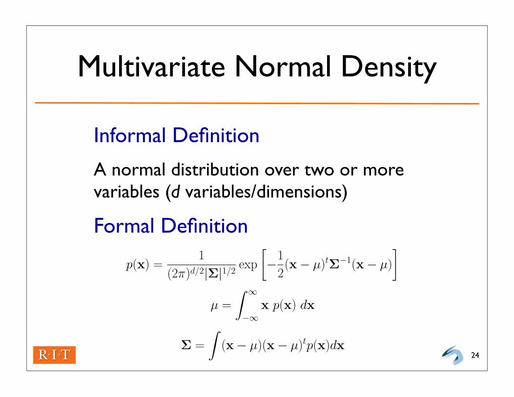
Multivariate Normal Density

Informal Definition

A normal distribution over two or more variables (d variables/dimensions)

Formal Definition

24


g(x) = P (!1|x)! P (!2|x)

g(x) = lnp(x|!1)

p(x|!2)+ ln

P (!1)

P (!2)


P (x) =1"2"#

exp

!!1

2

"x! µ

#

#2$

µ =

% #

!#x p(x) dx

#2 =

% #

!#(x! µ)2p(x) dx


p(x) =1

(2")d/2|!|1/2exp

&!1

2(x! µ)t!!1(x! µ)

'

µ =

% #

!#x p(x) dx

! =


3

bayesian decision theory - computer sciencerlaz/prec20092/slides/bayesiandecisiontheory.pdf ·...

Documents