beltstat v7.0 user manual
TRANSCRIPT
BELTSTAT v7.0
User Manual
December 2001
Revision 7.0.10
Conveyor Dynamics, Inc. 1111 West Holly, Street Bellingham WA, 98225
(360) 671-2200 www.conveyor-dynamics.com
2
1.0 INTRODUCTION ............................................................................................................................ 7
2.0 GETTING STARTED...................................................................................................................... 8
3.0 THE USER INTERFACE................................................................................................................ 9 3.1 OVERVIEW ...................................................................................................................................... 9 3.2 THE MAIN MENU & TOOLBAR ....................................................................................................... 9 3.3 FILE MENU .................................................................................................................................. 10 3.4 GENERAL - GENERAL PROJECT INFORMATION........................................................................... 12
3.4.1 Client Information ................................................................................................................ 12 3.4.2 Job Number .......................................................................................................................... 12 3.4.3 Designer ............................................................................................................................... 12 3.4.4 Description ........................................................................................................................... 12 3.4.5 Remarks ................................................................................................................................ 13 3.4.6 Input Units ............................................................................................................................ 13 3.4.7 Output Units ......................................................................................................................... 13 3.4.8 Analysis Type........................................................................................................................ 13 3.4.9 Output Curve Report ............................................................................................................ 13 3.4.10 Itemized Loss Table .............................................................................................................. 13
3.5 MATERIAL – MATERIAL PROPERTIES ........................................................................................ 14 3.5.1 Material Conveyed ............................................................................................................... 14 3.5.2 Design Tonnage.................................................................................................................... 14 3.5.3 Loading Multiplier................................................................................................................ 14 3.5.4 Allowed Cross Sectional Loading......................................................................................... 15 3.5.5 Bulk Density.......................................................................................................................... 15 3.5.6 Surcharge Angle ................................................................................................................... 15 3.5.7 Maximum Lump Size............................................................................................................. 15 3.5.8 Percent Lumps ...................................................................................................................... 15 3.5.9 Lump Shape Factor .............................................................................................................. 15 3.5.10 Chute Drop Distance ............................................................................................................ 15 3.5.11 Abrasive index ...................................................................................................................... 15 3.5.12 Environmental Condition...................................................................................................... 15 3.5.13 Maintenance Condition ........................................................................................................ 16 3.5.14 Hours in Service Per Day ..................................................................................................... 16 3.5.15 Minimum Temperature ......................................................................................................... 16 3.5.16 Maximum Temperature......................................................................................................... 16
3.6 BELT – BELT PROPERTIES............................................................................................................ 17 3.6.1 Belt Width ............................................................................................................................. 17 3.6.2 Belt Speed ............................................................................................................................. 17 3.6.3 Type of Carcass .................................................................................................................... 17 3.6.4 Belt Rating ............................................................................................................................ 17 3.6.5 Belt Weight ........................................................................................................................... 18 3.6.6 Top Cover Thickness ............................................................................................................ 18 3.6.7 Bottom Cover Thickness ....................................................................................................... 18 3.6.8 Elasticity ............................................................................................................................... 18 3.6.9 Allowable Sag ....................................................................................................................... 19 3.6.10 Edge Distance to Material.................................................................................................... 19
3.7 IDLER – IDLER PROPERTIES......................................................................................................... 20 3.7.1 Carry Side Trough Angle...................................................................................................... 20 3.7.2 Trough Angle - Return Side .................................................................................................. 20 3.7.3 Number of Rolls .................................................................................................................... 20 3.7.4 Idler Name / Series ............................................................................................................... 21 3.7.5 Roll Diameter ....................................................................................................................... 21 3.7.6 Seal Friction ......................................................................................................................... 21
3
3.7.7 Coulomb Friction Coefficient (CFC).................................................................................... 21 3.7.8 Rotating Weight .................................................................................................................... 21 3.7.9 Load Rating .......................................................................................................................... 21 3.7.10 Trough Shape Multiplier - Carry Side.................................................................................. 21 3.7.11 Trough Shape Multiplier - Return Side................................................................................. 22 3.7.12 Temperature Adjustment....................................................................................................... 22 3.7.13 (KX/KY) Regenerative Correction ........................................................................................ 22 3.7.14 Skirtboard Friction Factor ................................................................................................... 22 3.7.15 Skirtboard Width................................................................................................................... 23 3.7.16 Depth of Material Touching Skirtboard ............................................................................... 23 3.7.17 Vertical Installation Tolerance............................................................................................. 23 3.7.18 Use Drift Tensions for Radii................................................................................................. 23
3.8 DRIVES – CONVEYOR DRIVES/BRAKES & TAKE-UP PARAMETERS ............................................. 24 3.8.1 Motor Nameplate................................................................................................................. 24 3.8.2 Power Ratio .......................................................................................................................... 24 3.8.3 Motor Synchronous Speed .................................................................................................... 25 3.8.4 Starting Torque Limit Percent .............................................................................................. 25 3.8.5 Drive Inertia at Motor .......................................................................................................... 25 3.8.6 Drive Efficiency .................................................................................................................... 25 3.8.7 Drive Friction Factor (Running) .......................................................................................... 25 3.8.8 Drive Friction Factor (Accel/Decel) .................................................................................... 25 3.8.9 Brake Torque Ratio .............................................................................................................. 25 3.8.10 Acceleration Time................................................................................................................. 25 3.8.11 Braking Time ........................................................................................................................ 25 3.8.12 Total Brake Torque Ratio ..................................................................................................... 26 3.8.13 Drive Slip Percent ................................................................................................................ 26 3.8.14 Counterweight Type.............................................................................................................. 26 3.8.15 Gravity Take-up.................................................................................................................... 26 3.8.16 Fixed Take-up ....................................................................................................................... 26 3.8.17 Tension at Tension Device.................................................................................................... 26 3.8.18 Take-up Extension ................................................................................................................ 26
3.9 PROFILE – CONVEYOR PROFILE INPUT ....................................................................................... 27 3.9.1 Flight .................................................................................................................................... 28 3.9.2 Flight Number....................................................................................................................... 28 3.9.3 Ground X (or Station)........................................................................................................... 28 3.9.4 Ground Y (or Elevation) ....................................................................................................... 28 3.9.5 Flight Length ........................................................................................................................ 28 3.9.6 Flight Height ........................................................................................................................ 28 3.9.7 Idler Spacing ........................................................................................................................ 28 3.9.8 Flight ID ............................................................................................................................... 29 3.9.9 Load %.................................................................................................................................. 29 3.9.10 Conv. Load ........................................................................................................................... 29 3.9.11 Pulley Diameter.................................................................................................................... 29 3.9.12 Pulley Wrap .......................................................................................................................... 30 3.9.13 Vertical Curve Radius .......................................................................................................... 30 3.9.14 Horizontal Curve Radius ...................................................................................................... 30 3.9.15 Concentrated Weight Specification ...................................................................................... 30 3.9.16 Miscellaneous Drag Tension Specification .......................................................................... 30 3.9.17 Notes ..................................................................................................................................... 30
3.10 QUICK START WINDOW..................................................................................................................... 31 4.0 BELTSTAT OUTPUT FILE AND RESULTS WINDOW ......................................................... 32
4.1 MATERIAL SPECIFICATIONS .......................................................................................................... 33 4.2 BELT SPECIFICATIONS ................................................................................................................... 34 4.3 IDLER AND ANCILLARY SPECIFICATIONS ...................................................................................... 36 4.4 MOTOR / REDUCER / BRAKE SPECIFICATIONS............................................................................... 38

4
4.5 TENSION SPECIFICATIONS AND "TENSION" WINDOW........................................................... 40 4.6 "TENSION RATIO" – DRIVE / BRAKE TENSION RATIOS.................................................................. 42 4.7 "TAKE-UP" SPECIFICATIONS.......................................................................................................... 43 4.8 FORCE / DRAG SUMMARY ............................................................................................................. 47 4.9 CONVEYOR SUMMARY .................................................................................................................. 47 4.10 THE RESULTS WINDOW WITH THE "PLOT" BUTTON SELECTED..................................................... 48 4.11 THE RESULTS WINDOW WITH THE "MAIN" BUTTON SELECTED .................................................... 49
4.11.1 "Summary" Window Selection Button................................................................................... 49 4.11.2 "Tension" Window Selection Button ..................................................................................... 49 4.11.3 "Concave" Window Selection Buttons .................................................................................. 50 4.11.4 "Convex" Window Selection Buttons .................................................................................... 51 4.11.5 "Loss Table" Window Selection Buttons............................................................................... 52
4.12 VIEW BSO FILE ............................................................................................................................ 53 5.0 PROFESSIONAL VERSION FEATURES.................................................................................. 54
5.1 PROJECT FILES .............................................................................................................................. 54 5.1.1 Project Files - Input Table.................................................................................................... 55 5.1.2 Project Files - Results Table................................................................................................. 58 5.1.3 Project Files - Tension Table ............................................................................................... 59
5.3 SPLICE PATTERN ........................................................................................................................... 69 5.4 BELT TURNOVER CALCULATIONS ................................................................................................. 73 5.5 TRANSITION LENGTHS................................................................................................................... 81 5.6 MATERIAL TRAJECTORY ............................................................................................................... 82 5.7 BELT ROLL CALCULATIONS ................................................................................................................ 83 5.8 MATERIAL LOADING PROFILE ............................................................................................................. 84 5.9 BELT FEEDERS .............................................................................................................................. 84 5.10 PULLEY DESIGN ............................................................................................................................ 85 5.11 IDLER MASS CALCULATIONS..................................................................................................... 89 5.12 LOADING ON/OFF ............................................................................................................................. 90 5.13 MULTIPLE DESIGN RUNS............................................................................................................... 91 5.14 MICROSOFT WORK REPORTS..................................................................................................... 93
6.0 EXAMPLES.................................................................................................................................... 95 6.1 EXAMPLE #1.................................................................................................................................. 96 6.2 EXAMPLE #2................................................................................................................................ 108 6.3 EXAMPLE #3................................................................................................................................ 120 6.4 EXAMPLE #4................................................................................................................................ 131 6.5 EXAMPLE #5 – FIXED TAKE-UP................................................................................................... 141

5
Foreword
ALL RIGHTS RESERVED. No part of this documentation may be reproduced in any form, by any means, without the prior written permission of Conveyor Dynamics, Inc. (CDI) U.S.A. CDI makes no representations or warranties with respect to the program material and specifically disclaims any implied warranties, accuracy, merchantability or fitness for any particular purpose. Further, CDI reserves the right to revise the program material and to make changes therein from time to time without obligation to notify purchaser of any revisions or changes except specific errors determined to be incorporated in the program material. It shall be the responsibility of CDI to correct any such errors in an expeditious manner. In no event shall CDI be liable for any incidental, indirect, special or consequential damages arising out of the purchaser’s use of program material.
6

7
1.0 INTRODUCTION BELTSTAT is a computer program used in the design of troughed belt conveyors handling bulk materials. BELTSTAT can analyze conveyors of any length and topography having up to twelve drive/brake stations, without restriction as to location. The program can analyze downhill, regenerative conveyors, and belt widths from 24 to 120 inches. Drives may be conventional head type, tail, and/or intermediate (TT-type) drives of any combination. Both acceleration and braking action can be analyzed using either independently controlled starting/stopping times or controlled acceleration/braking force. Starting and stopping forces may be proportioned as desired among the multiple drives. BELTSTAT is intended to be a design tool and computational aid to competent and experienced conveyor design engineers. Correctly employing the program together with good engineering judgment and conveyor design experience, users can quickly arrive at the following conveyor design data: o Belt width and speed o Belt tension rating o Counterweight tension o Horsepower rating of drive motors o Drive motor starting characteristics o Idler specifications and spacing o Pulley and shaft design o Vertical curve radii and required special idler spacing o Brake size (if required) o Flywheel requirements (if applicable) BELTSTAT has been verified against successfully operating conveyor systems. When used by an engineer familiar with conveyor design methods, the program functions as a powerful design tool, providing uniform, accurate, and rapid computations. The program allows the engineer to easily explore alternative configurations, such as alternate counterweight and drive locations, which may result in a more economical design. The formulae and calculation methods of BELTSTAT are based upon the methods and data published by the Conveyor Equipment Manufacturers Association (CEMA). Selected methods have been modified or expanded to meet the requirements of high capacity, high speed, and overland systems. Finally, BELTSTAT is designed to provide flexibility and convenience to the engineer. Where possible, input parameters are optional. If the user does not specify these, the program will either use an appropriate default value or make a selection based on the known variables. BELTSTAT operates by reading an input file, analyzing the data, and then writing the final calculations to an output file. The User Interface is a different program which allows the user to easily interact with BELTSTAT. The User Interface allows you to input the conveyor geometry, and all the needed parameters for the BELTSTAT input file. It will then write the input file for BELTSTAT, and allow you to run BELTSTAT. The manual consists of six chapters. Chapter 2 describes how to set up BELTSTAT on your computer, and details the necessary files and equipment needed for the program to run. Chapter 3 presents the User Interface that allows you to input the parameters needed for BELTSTAT. Then, Chapter 4 explains the BELTSTAT results windows and output file. Chapter 5 discusses the advanced features found in the professional version. Finally, Chapter 6 contains examples of conveyor designs made with BELTSTAT and steps the user through each stage of the design. Many users may wish to skip directly to the example section, and only reference the main body of the user manual as required.
8
2.0 GETTING STARTED Before proceeding be sure you have the following items.
1. BELTSTAT v7.0 CD-ROM 2. Hardware key (dongel) 3. BELTSTAT User Manual
The BELTSTAT CD-ROM contains the following directories:
1. “INSTALL” – The installation directory with the BELTSTAT SETUP.EXE File 2. “SUPERPRO” – Directory containing software for the BELTSTAT hardware key. 3. “EXAMPLES” – A copy of the Examples files found in Chapter 6. This directory is also
copied onto your hard drive under the /BELTSTAT/EXAMPLES installation directory.
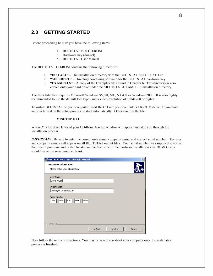
The User Interface requires Microsoft Windows 95, 98, ME, NT 4.0, or Windows 2000. It is also highly recommended to use the default font types and a video resolution of 1024x768 or higher. To install BELTSTAT on your computer insert the CD into your computers CR-ROM drive. If you have autorun turned on the setup process be start automatically. Otherwise run the file: X:/SETUP.EXE Where X is the drive letter of your CD-Rom. A setup window will appear and step you through the installation process. IMPORTANT: Be sure to enter the correct user name, company name, and correct serial number. The user and company names will appear on all BELTSTAT output files. Your serial number was supplied to you at the time of purchase and is also located on the front side of the hardware installation key. DEMO users should leave the serial number blank.
Now follow the online instructions. You may be asked to re-boot your computer once the installation process is finished.

9
3.0 THE USER INTERFACE
3.1 Overview The new BELTSTAT user interface is shown below. It contains various input and output windows. These windows allow the user to quickly build, analyze, and optimize complex conveyor systems. Each window will be briefly described in the following sections.
3.2 The Main Menu & Toolbar The “Main Menu” contains groups of pulldown lists. These lists give the user access to all the program features. The “pictures” on the toolbar menu provide quick access to many of the most commonly used items. Both the main menu and toolbar are shown below.

10
3.3 FILE Menu The “File” main menu list contains common file operation commands and output features found in most windows based programs. The “File” menu pulldown list is shown below.
New File
Opens the "Conveyor Quick Start" window to begin working with a new BELTSTAT file.
Open File Opens an existing file.
Save File
Saves the file using the current filename. The file is also automatically saved each time the BELTSTAT calculations are run.
Save File As
Save the file under a different filename Close File
Closes the current file. If the file has not been saved it will prompt the user to save the file. Open / Save Project
These features are only available in the professional version of BELTSTAT. When designing a conveyor the engineer must be aware of several different “worst cases” design scenarios. For example, a conveyor with only the inclined, or declined sections loaded will behave very differently and a separate BELTSTAT file should be created for each case. These multiple files can be saved as a single "Project". The user can now automatically open ALL files in a project at once instead of having to open each file one at a time. Furthermore, using the “Project” menu these files can all be created automatically (this is discussed in detail in chapter 5). The Project file also contains the

11
"Standard Cases" Input table parameters, thereby restoring any information used to create the project.
Close All Files and Projects
Closes all opened files and projects. If a file has not been saved it will prompt the user to save the file.
Print Current Window
Prints the currently selected window. This window maybe the BSO results window or any of the “Report” windows (trajectory, flap, turnover, cases summary, etc.)
Print BSO File
Prints the results (*.BSO) file.
Print Conveyor Report Allows the user to quickly print out specific information on all currently opened files.
Windows Options
Show Toolbar – Turns the main toolbar on and off. Close Input Window on Exit – Close the current input window when another input window is selected. Save Window Sizes and Positions – Save the current window sizes and the positions as the global defaults for BELTSTAT.
Save & Close Current Window – Simple saves and closes the current input window.
Undo Changes to Window – Undoes any changes to the current window.
Opened Windows – Shows a list of all opened windows.
Plotting Options
Set information pertaining to the BELTSTAT output plots. Show Absolute Tension Values – Sets whether the tension values are plotted as absolute values (N or LBS) or as belt rating values (N/mm or PIW). Show Station Numbers – Turns the station numbers on and off in the plot window. Show Drive / Brake Symbols – Turns the drive /brake symbols on and off in the plot window. Show 2nd Plot Window – Shows a 2nd Plot window. This allows the user to view the BELTSTAT plots and summary table at the same time. Use User Default Plots – Uses the user default plots. Save Default Plots – Save the current plot configuration as the user default.

12
RUN Save the current file and runs the BELTSTAT calculations.
Recent Files List
List the last four files recently used. Selecting a file automatically opens the file.
Exit Exits the BELTSTAT program
3.4 GENERAL - General Project Information The identification menu allows you to enter information about the conveyor, client, designer, etc. Each option is limited to the space in the box, except for the conveyor description box which is longer than it appears. The information placed in these boxes will be printed at the top of each page in the output file. It is also used as the title blocks for the tension plots made in the plot menu. The input units box controls how BELTSTAT interprets the data that you enter in the user interface. All parameters must be entered in the same units. Also, if you change the unit type the user interface does not change the values of the parameters which you have already entered. However, the unit labels do change for each parameter. Be careful to enter the conveyor parameters in the correct units.
3.4.1 Client Information Enter the clients name here (optional).
3.4.2 Job Number Enter the job number here (optional).
3.4.3 Designer Enter the name of the designer (optional). This field Defaults to the "User Name" specified when installing the BELTSTAT program.
3.4.4 Description Enter a description of the conveyor (optional). This information is also added to the bottom of each of the conveyor output tension plots.

13
3.4.5 Remarks Enter any general remarks you feel relevant about the conveyor here (optional). This information is also added to the bottom of each of the conveyor output tension plots.
3.4.6 Input Units The input units box control how BELTSTAT interprets the data that you enter in the user interface. All parameters must be entered in the same unit system. Also, if you change the unit type, the user interface does not change the values of the parameters which you have already entered. However, the unit labels do change for each parameter. Be careful to enter the conveyor parameters in the correct units.
3.4.7 Output Units The output units allows you to choose the whether the output file will be written in English or Metric units. These units may differ from the input units.
3.4.8 Analysis Type This field tells BELTSTAT how to calculate the KY values.
CEMA The KY values will be calculated according to a modified CEMA KY formula. Behren's and Schwartz The KY values will be calculated according to KY calculations formulated by Behren's and Schwartz. On large belts or belts with large idler spacing (greater than 6.0 feet), this analysis type is suggested regardless of belt construction. Rheological Analysis This analysis type is not currently marketed in BELTSTAT. Contact Conveyor Dynamics if you are interested in more information about this analysis method.
3.4.9 Output Curve Report Indicates whether or not a detailed curve report will be generated in the BELTSTAT output file.
3.4.10 Itemized Loss Table When this box is selected a BELTSTAT itemized loss table is created showing where losses occur.

14
3.5 MATERIAL – Material Properties The material menu allows you to enter the necessary information about the material being conveyed. The “TAB” key moves between input lines (SHIFT-TAB moves back one line).
3.5.1 Material Conveyed This field contains a description of the material being conveyed and has a pulldown submenu. Click on the <down arrow> to see the available selections (coal, tar sand, copper ore, etc.). When a material is chosen from the list its default properties will automatically be entered into the remaining fields. The user is not limited to the default materials and may type in ANY material type and its corresponding properties. Furthermore, by selecting, “CREATE A NEW MATERIAL”, or “DELETE A MATERIAL” the user can add to, or remove, items from the default pulldown list.
3.5.2 Design Tonnage Desired conveyor design capacity in tons per hour (metric) or short tons per hour (English), wet or dry. Input value sets the belt size, speed, and material load on the belt. This field has no default, and must be set by the user.
3.5.3 Loading Multiplier The flight loading multiplier acts as a multiplying factor on each flight's loading. This is useful for evaluating a partially loaded, overloaded, or empty conveyor. For example, a flight loading

15
multiplier equal to zero will result in an empty-belt analysis. A multiplier of 0.5 will cause all flight loading percentage to be reduced by half of their input value.
3.5.4 Allowed Cross Sectional Loading Maximum allowable material cross-sectional loading, as defined by CEMA. The program will select belt width, speed, and material edge clearance (unless these have been input) such that this loading will not be exceeded. Default value is 85 percent.
3.5.5 Bulk Density The bulk density of the material as defined by CEMA.
3.5.6 Surcharge Angle Dynamic angle of repose as defined by CEMA. The default value is 20 degrees.
3.5.7 Maximum Lump Size Maximum lump size is used to compute impact force at belt transfer and to indicate minimum CEMA belt width when used in conjunction with percent lumps. Default value is 20 percent.
3.5.8 Percent Lumps Percent lumps as defined by CEMA. Used in conjunction with maximum lump size and with CEMA idler selection. Default value is 20 percent.
3.5.9 Lump Shape Factor Although not described in CEMA, this factor can be found in the "Engineering Handbook - Conveyor and Elevator Belting," by B. F. Goodrich Company. The factor is used to estimate lump weight for calculation of loading station impact force. The factor describes the shape of the lump. For a material with cubic shaped lumps, the factor would be equal to 1.0. With long Slabby lumps, the factor would be 1.25. Default value is 1.4.
3.5.10 Chute Drop Distance The height the material drops before contacting the belt at the loading station. This is used for calculation of loading station impact force.
3.5.11 Abrasive index Describes the abrasive characteristics of the material. This field has a submenu selection, which are:
Selection Meaning
1 none 2 light 3 moderate 4 very 5 extreme
The default selection is 4.
3.5.12 Environmental Condition This variable indicates the cleanliness of the environment. The allowable input conditions are: CLEAN, MODERATE, and DIRTY. This factor is used in idler selection and rating per CEMA. Default value is DIRTY.

16
3.5.13 Maintenance Condition This variable describes the expected idler maintenance conditions. Allowable inputs are GOOD, FAIR, or POOR. This factor is used in idler selection and idler rating per CEMA. The default value is POOR.
3.5.14 Hours in Service Per Day This factor is used in idler selection and rating per CEMA. Default value is 24 hours.
3.5.15 Minimum Temperature This variable is the temperature used to evaluate the CEMA KT value, the ambient temperature correction factor. Above 32° F, KT is equal to 1.0. The user is advised to input a temperature at 32° F or higher when executing a low-friction analysis. Default value is 30° F.
3.5.16 Maximum Temperature This variable is used to obtain the total temperature change, and subsequently, the take-up travel due to temperature change. Default value is 100° F.

17
3.6 BELT – Belt Properties The belt menu contains the necessary information for the belt specification. The procedure for the belt parameters is very much the same as those for the material parameters. The fields which have submenu selections are “belt width” and “type of carcass”. The width of the belt can be from 18 inches to 120 inches. The belt carcass can be steel, polyester, nylon, or left blank. Those fields which are left blank will be calculated by BELTSTAT. For example, if the belt width and strength are not specified then BELTSTAT will determine the width and strength needed for the required tonnage, and conveyor profile. However, there are some fields which require the input from the user. The “Sag Allowable on Carry Side, %” must be entered by the user.
3.6.1 Belt Width The user may specify the belt width or allow the program to select it. Any belt width from 18 inches up to 120 inches, including nonstandard widths in this range, may be input by the user. If not input, a selection will be made from the following values: 24, 30, 36, 42, 48, 54, 60, 66, 72, 84, 90, 96, 102, 108, 114, 120 (inches - for English units).
3.6.2 Belt Speed The belt speed may be input or the user may allow the program to calculate it. The program selection will be based on minimum edge distance, maximum allowable percentage loading, and belt width. If neither belt width nor speed are input, the program will select the narrowest belt width for which the required speed does not exceed 20 times the belt width in inches or 1200 FPM.
3.6.3 Type of Carcass The user may specify POLYESTER, NYLON, or STEEL, or allow the program to select (leave blank). If not input, the program will select polyester carcass unless the running stress exceeds 800 PIW, in which case the program will select steel cable.
3.6.4 Belt Rating The user may specify or allow the program to select this parameter. Unless input, the program will select a belt strength to meet the maximum "RUNNING" tension base on a factor of safety of 6.7

18
(for steel cable belts). The selected PIW will be to the next higher 25 PIW increment for fabric and 100 PIW for steel cable belt.
3.6.5 Belt Weight The user may specify or allow the program to select the belt weight. The program computes the weights for polyester, nylon, and steel cable belting. Cover weights are calculated separately and then added to the carcass weights to produce the total belt weight.
3.6.6 Top Cover Thickness This variable refers to the thickness of gum rubber above the conveyor belt carcass. For steel cable belts, the top cover thickness is interpreted as the thickness from the top of the steel cables to the top surface of the belt cover. The top cover thickness is used by the program in computing the belt weight when belt weight has not been input.
If the user does not input the top cover thickness, the program will compute a suitable thickness based on abrasiveness of the conveyed material, lump size, percentage of lumps, operating hours per day, belt speed, and belt tape length. This formulation is based in part, on the Goodyear "red handbook." Also, the following minimum thickness is maintained for load support and rubber support around high tension pulleys:
CARCASS MATERIAL PIW MIN. TOP COVER (IN.) Fabric All 0.1875 Steel Cable Up to 2700 0.2500 Steel Cable 2701 to 3500 0.3125 Steel Cable Over 3500 0.3750
If any unusual conditions of abrasion are anticipated, the user is advised to input the appropriate thickness, based on judgment and/or belt manufacturer's recommendations.
3.6.7 Bottom Cover Thickness This variable refers to the thickness of gum rubber below the conveyor belt carcass. For steel cable belts it is interpreted as the thickness from the bottom of the steel cables to the bottom surface of the belt cover. As with the top cover thickness, the bottom cover thickness is used in the computation of the belt weight when it has not been input.
If the user does not input a value, the program will select a value not less than one-third of the top cover thickness, rounded to the nearest 1/32-inch. Also, the following minimums are applied for steel cable belting:
PIW MIN. BOTTOM COVER (IN.) Up to 3500 0.2500 Over 3500 0.3125
3.6.8 Elasticity This input variable represents the elastic modulus of the conveyor belt and is used in curve computations and in take-up travel computations. This is the TOTAL elasticity of the belt in LBS and not PIW (N not N/mm). If not input, the program will compute an approximate value based on the carcass material, carcass rating, and belt width. Conveyor belt elasticity may vary considerably among different

19
manufacturers, so the user is advised to input the manufacturers specified value, once a vendor selection has been made.
3.6.9 Allowable Sag The user may specify the maximum allowable Catenary sag between idlers. The value is computed and set as a governing criterion for each geometric flight described later. Default value is 1.5 percent on carry side or absolute distance of 2/3 idler roll diameter of carry or return side.
3.6.10 Edge Distance to Material The interpretation of the edge distance is according to CEMA, and refers to the minimum distance to be maintained from the edge of the belt to the theoretical material cross-section when operating at the rated tonnage. If this variable is not input, and no value is input for the cross-sectional design loading, the program will select a minimum value based on lump size, surcharge angle, trough angle and belt width. In all cases where belt speed and/or width are input, these values are maintained. Therefore, if both speed and width are input, the edge distance is fixed, and the value input for edge distance is ignored. When the cross-sectional design loading and edge distance are both input, both are used in selecting belt width and speed (unless both are input). The program selection will meet both criteria.

20
3.7 IDLER – Idler Properties The idler and ancillary specifications menu contains the necessary specifications for the idlers, and other parameters. In this menu, only the trough angle and series number have submenu selections. If you choose a standard idler from the series number submenu or leave this field blank then the input in fields 3A through 3E will be ignored by BELTSTAT. If you wish to enter customized values in the 3A through 3E fields, then you must enter a series number not available in the series number submenu. Those field which are left blank will be calculated from the known information. For example, the idler series number will be calculated from then tension and other requirements in the belt, then the parameters which depend on the series number (3A through 3E) will be calculated from the idler series number.
3.7.1 Carry Side Trough Angle The user may input any desired trough angle, including nonstandard angles, or allow the program to select. Only one trough angle may be specified for the full length of the conveyor. Default value is 35 degrees.
3.7.2 Trough Angle - Return Side This variable refers to the angle of incline of the idler rolls on the V-return type idlers. If not input, flat return idlers are assumed.
3.7.3 Number of Rolls Number of rollers in the idler set.

21
3.7.4 Idler Name / Series The user may input a standard CEMA series (e.g. C6) or allow the program to select. This field has a submenu selection available, move the cursor to this field and press <ENTER> to see the list. If the series number field is left blank or a standard series is input from the submenu, then the program will ignore the input in field 3A to 3E. To be able to input a nonstandard series you must input the name of the nonstandard series or enter the word OTHER in the field. If the user enters a series which is not a CEMA standard, he must specify the idler roller diameter, seal friction, coulomb friction, viscous drag, rotating weight, load rating, and the number of rollers. If the program is required to select an idler series, the maximum idler spacing will be selected within CEMA load rating for the idler class. The CEMA class sizes are A4, A5, B4, B5, C4, C5, C6, D5, D6, E6, and E7.
3.7.5 Roll Diameter May be input for nonstandard idler series.
3.7.6 Seal Friction Seal friction (Ai), as defined by CEMA, may be input for nonstandard idler series. The seal friction is evaluated per CEMA for standard CEMA Idler Series.
3.7.7 Coulomb Friction Coefficient (CFC) The Coulomb friction factor (KX), as defined by CEMA, is the frictional resistance of idler rolls to rotation and sliding resistance between the belt and the idler rolls. The Coulomb friction factor is evaluated per CEMA for standard CEMA Idler Series. Kx = CFC * (Wb + Wm) + Ai / Si The CEMA default value is 0.00068
3.7.8 Rotating Weight The user may input the rotating weight referenced to the belt line. This may be input for nonstandard idler series only. The rotating weight is evaluated per CEMA for standard CEMA idler series.
3.7.9 Load Rating The user may input the idler load rating for nonstandard idler series. Otherwise, the value for the CEMA series is used. The load rating is then corrected by the program, according to CEMA formulae, using the lump adjustment factor, environmental and maintenance factors, service factor, and belt speed correction factor.
3.7.10 Trough Shape Multiplier - Carry Side CEMA makes no adjustment for the change in the carry idler trough shape. Field tests have shown that there is an increase in the KY value due to added belt hysteresis losses in the angle transition zone. For fabric belt, the program will compute an adjustment multiplier and take the product of the base KY and the multiplier as the new KY value, shown in the table below. The KY formulae for steel cable belting take the idler angle into account, and so the program will select a KY multiplier value of 1.00. If the user inputs a value it will override the program selection.
Idler Angle (degrees) KY Multiplier (fabric belt)
0 .90 20 1.00 35 1.075 45 1.125

22
Suggestions: A) When analyzing for the highest friction condition, allow the program to select a value. However, when analyzing with ambient temperature below -10 degrees Fahrenheit, input a value of 1.00. B) When analyzing for the lowest friction condition (e.g. Regenerative conveyor), input a value of 1.00.
3.7.11 Trough Shape Multiplier - Return Side CEMA return side friction factors make no allowance for the return idler incline angle (i.e. V-return idlers). No representative field data has been compiled to evaluate the relationship between the return idler angle and return side friction factors. Nevertheless, the program will compute a friction factor multiplier for return idlers. The value will be 1.00 for flat idlers. Any input by the user will override the program selection.
3.7.12 Temperature Adjustment Ambient temperature correction factor (KT) is the idler rotational and flexing resistance increase of the belt in cold weather operation. This is computed according to the CEMA data. The minimum ambient temperature is used as the basis for computing this factor. Above 32 degrees F, the KT factor is equal to 1.00.
3.7.13 (KX/KY) Regenerative Correction CEMA recommends that when analyzing a regenerative (downhill; power-generating) conveyor or when computing the longest expected drift time, a reduction factor be applied to KX and KY. CEMA recommends that the KY and KX values be multiplied by 0.666 and that the idler bearing seal friction, skirtboard rubber friction, and belt scraper friction be set to zero.
If the user desires this type of low-friction case, he should input a value of 0.666 (or other value dictated by his judgment). The value input will be applied to the KY and KX factors. Also, if the program detects an input value less than one, idler and pulley bearing seal friction, skirtboard rubber friction, and scraper friction will be set to zero.
3.7.14 Skirtboard Friction Factor Per CEMA, the program will accept input for the skirtboard coefficient of friction for the material conveyed. The value is used per CEMA Fifth Edition. The default value is .06, which is the average value for coal. The program internally adds 3 pounds per foot for the friction of the skirtboard rubber. The skirt length is geometric input.

23
Alumina, pulv. dry 0.1210 Coke, ground fine 0.0452 Limestone pulv., dry 0.1280
Ashes, coal, dry 0.0571 Coke, lumps and fines 0.0186 Magnesium chloride, dry 0.0278
Bauxfte, ground 0.1881 Copra, lumpy 0.0203 Oats 0.0219
Beans, navy, dry 0.0798 Cullet 0.0836 Phosphate rock, dry, broken 0.1086
Borax 0.0734 Flour, wheat 0.0265 Salt, common, dry, fine 0.0814
Bran, granular 0.0238 Grains, wheat, corn or rye 0.0433 Sand, dry, bank 0.1378
Cement Portland, dry 0.2120 Gravel, bank run 0.1145 Sawdust dry 0.0086
Cement clinker 0.1228 Gypsum, 1/2" screenings 0.0900 Soda ash, heavy 0.0705
Clay, ceramic, dry fines 0.0924 Iron ore, 200 lbs./cu ft 0.2760 Starch small lumps 0.0623
Coal, anthracite, sized 0.0538 Lime, burned, 1/8" 0.1166 Sugar, granulated dry 0.0349
Coal, bituminous, mined 0.0754 Lime hydrated 0.0490 Wood chips, hogged fuel 0.0095
3.7.15 Skirtboard Width Per CEMA, the program will compute a skirtboard width of 2/3 the belt width. The designer may input other width selections. This value is used to calculate the depth of the material touching the skirtboard and the resulting frictional forces.
3.7.16 Depth of Material Touching Skirtboard The depth of the material touching the skirtboard (factor "Hs" in CEMA). If left blank, the program will assume a material surcharge angle of zero and thus calculate the maximum possible depth of material which can contact the skirtboard. This factor will override the depth calculated by the above skirtboard width.
3.7.17 Vertical Installation Tolerance The maximum possible vertical misalignment of the idlers from the ideal belt line elevation. The tolerance is interpreted as a possible plus or minus value. This variable is used in sizing convex vertical curves and in determining the maximum load per idler on convex curves. To do this, an idler on the curve is assumed to be elevated above its ideal position by the full value of the installation tolerance, and the two adjacent idlers are assumed to be lowered by the same amount. This is considered the worst case with respect to idler loading.
The program attempts to size the convex curve such that the idler capacity is not exceeded. However under certain conditions, this is not possible and the program will show an overload condition. If this occurs, the user must make the necessary corrections to the idler capacity, installation tolerance, belt tension, or curve radius.
3.7.18 Use Drift Tensions for Radii For certain conveyors, the drift tension condition may never occur. An example would be a conveyor which is always started and/or stopped using controlled braking and driving forces. For these cases, the conveyor designer may specify that the drift tensions as calculated by the program shall not be used in vertical curve radius selection. If the drift time and tensions are used, the vertical curve selections will evaluate the minimum and maximum, carry and return side tensions for vertical curve selection criteria.

24
3.8 DRIVES – Conveyor Drives/Brakes & Take-up Parameters The user may specify the motor nameplate horsepower at each station or allow the program to select a motor size based on running horsepower. This variable represents the total nameplate horsepower at each drive station, regardless of whether the drive pulley is driven by one or two motors. The program has a motor selection range from 1 to 10,000 HP.
3.8.1 Motor Nameplate The user may specify the motor nameplate horsepower at each station or allow the program to select the motor sized based on running horsepower. The variable represents the total nameplate horsepower at each drive station, regardless of whether the drive pulley is driven by one or two motors. The program has a motor selection range from 1 to 10,000 HP (7457 kW).
3.8.2 Power Ratio This variable represents the distribution of the total running brake horsepower among the drive pulley stations. This factor is not applicable to conveyors with one drive station only. The ratios may be input in any manner that describes the distribution, such as the following examples:
Examples (a) 1:1 - Two drive pulleys with equal power. (b) 0.5:0.5 - Same as (a) above. (c) 1:1:1 - Three drive pulleys with equal power. (d) 2:1 - Two drive pulleys with twice primary power with respect to secondary pulley.

25
(e) 3:2:1 - Three drive pulleys with three times primary power, twice secondary power with respect to tertiary drive pulley. (f) 1:0 - One drive pulley and one brake pulley.
The default is equal power distribution.
3.8.3 Motor Synchronous Speed This factor, in conjunction with the belt speed and drive pulley diameter, is used to determine the gearbox ratio, and the drive inertia. Any value is acceptable for brakes or drives. Default value is 1800 RPM.
3.8.4 Starting Torque Limit Percent This input value specifies the ratio of motor starting torque to motor nameplate torque. This is used by the program to determine belt tensions during acceleration and acceleration time. If the user specifies the acceleration time, the starting torque limit is then calculated based upon the acceleration time as input. The default is 135 percent.
3.8.5 Drive Inertia at Motor Drive inertia represents the rotational moment of inertia of all motors, gearboxes and brakes located at the given drive/brake station. These are referenced to the highspeed shaft. If not input, the program will calculate the inertia of the motor and gearbox. This input can also be used to simulate flywheel effects if required.
3.8.6 Drive Efficiency This variable represents the efficiency of the gearbox at the given drive/brake station. Default value is 95 percent.
3.8.7 Drive Friction Factor (Running) This variable represents the coefficient of friction between the conveyor belt and the drive pulley. For lagged drive pulleys, default value is 0.35.
3.8.8 Drive Friction Factor (Accel/Decel) The Acceleration and Decelerating drive friction factor is the same as the running drive friction factor. The default value is .40.
3.8.9 Brake Torque Ratio Like the power ratio, the brake torque ratio determines the distribution of brake torque among drive stations. The brake can be a low speed brake direct coupled to the pulley, or highspeed coupled through a gearbox. Default value is 1:1:1 equal distribution among referenced stations.
3.8.10 Acceleration Time The user may specify acceleration time. If so, the motor starting torque will be determined to give this acceleration time. Belt tensions during acceleration will also be determined by the time input. If no acceleration time is input, the program computes it based upon the motor starting torque.
3.8.11 Braking Time Similar to acceleration time, the braking time represents the number of seconds in which the conveyor is stopped from the full speed. This is used to determine belt tensions during braking as well as brake torque requirements. If no braking time is input, the program computes it based on the total brake torque.

26
3.8.12 Total Brake Torque Ratio This variable represents the total available torque for braking. This is expressed as a percentage of the total motor nameplate torque of all motor/brake stations. The braking torque is distributed among the drive/brake stations according to the brake torque ratio.
3.8.13 Drive Slip Percent The speed at which the motor is at full load torque is determined by the drive slip. This is computed by the following formula: RPM Full Load Torque = (1 - Drive Slip%) * RPM Motor Synchronous Speed The default value is 1.944%.
3.8.14 Counterweight Type The counterweight type may be either fixed or a gravity type. If no input the program will assume a gravity type counterweight.
3.8.15 Gravity Take-up A gravity take-up has constant belt line tensions and variable displacement. The input take-up extension is not meaningful for a gravity take-up.
3.8.16 Fixed Take-up A fixed take-up is a conveyor belt tensioning device that does not allow movement of the take-up pulley. Consequently, the belt tension at the take-up pulley varies during different loading or starting and stopping conditions. Belt mass must be input for a fixed take-up.
3.8.17 Tension at Tension Device This variable allows the user to specify the belt tension at the counterweight. This tension will be held constant under acceleration, braking and drift conditions, acting as a gravity-type counterweight. If not input, the program will set the counterweight tension as required for belt sag and drive wrap conditions during running only. Wrap conditions during acceleration and braking will be output, but it is the responsibility of the user to see that the counterweight tension is sufficient to satisfy the wrap and sag criteria during acceleration and braking. Frequently, subsequent runs are required in which the value of the counterweight tension is input. The counterweight criteria for the acceleration, braking and drift cases are integrated with the pulley wrap angle, the system and/or drive masses, acceleration, braking and drift times. The many alternatives available to the designer make it impracticable for computer selection.
3.8.18 Take-up Extension Allows the user to input a fix take-up extension. This field is ignored if the take-up is gravity.

27
3.9 PROFILE – Conveyor Profile Input The program requires the user to input the conveyor configuration in an explicit manner, which will be described below. See Example #2 for a quick tutorial on creating a complete conveyor profile. Certain flights are necessary for any conveyor analysis. These are the head pulley location, drive/brake locations as applicable, and take-up location consisting of entering belt, take-up pulley, and exiting belt.

28
3.9.1 Flight A section of conveyor, which the designer wishes to configure in a manner different from any adjacent section of conveyor for one or more of the following reasons: a) Change of conveyor slope b) Change of material loading c) Change of skirtboard conditions d) Change of idler spacing e) Evaluate vertical curves f) Add/delete concentrated drag force g) Evaluate forces for structural criteria h) Evaluate belt tension forces for pulley design (e.g., drives Take-up, bend; tail) i) Determine accurate accounting of idlers and belt length j) Take-up zone k) Select pulley diameter, shaft and bearing size, mass and local bearing drag The first flight on any conveyor is located at the tail. All belt tension results are reported at the beginning of the flight. For example, the tension at the beginning of flight #5 will be reported in flight row #5. The tension at the end of flight #5 will be given in flight row #6 (the end of flight 5 is the beginning of flight 6).
3.9.2 Flight Number An index number given to each unique conveyor flight.
3.9.3 Ground X (or Station) The absolute X position (referenced to the first flight) of the beginning of the conveyor flight. It is often more convenient to specify the Ground X & Y Position of each conveyor flight than to specify the Flight Length and Height. Note: The user may input the Ground X & Ground Y data, or Flight Length and Flight Height data. It is simply a matter of whatever is most convenient.
3.9.4 Ground Y (or Elevation) The absolute Y position (referenced to the first flight) of the beginning of the conveyor flight.
3.9.5 Flight Length Length of the specific flight. The conveyors flight length is the horizontal projected length of the flight measured in feet (or meters). The true length is calculated internally in the program.
3.9.6 Flight Height Vertical rise of each specific flight. If there is no input, a height of zero is used. Up elevation is positive and down elevation is negative.
3.9.7 Idler Spacing Idler spacing can be specified or left blank to allow selection by the computer program. For flights which have no idlers, the user must enter "NONE" or "N". CEMA formulae for KY have been extrapolated to idler spacing up to 10 feet. Input of idler spacing over 10 feet may yield inaccurate friction factors.

29
3.9.8 Flight ID The flight ID tells the program what "type" of element the flight is. Valid Options are.
A " S" in this column indicates the existence of a skirtboard at the given flight. The skirtboard is assumed to extend along the entire length of the flight. A "D" indicates the location of a drive/brake station. The program interprets a drive station as occurring across a single conveyor flight. The program will allow any location on the conveyor exclusive of the Take-up. When entering the "D" the program will automatically assign a number to the drive station, i.e. "D1" for the first drive station, "D2" for the second, and so on. Input parameters for each drive station are found under the "Conveyor Drives/Brakes & Take-up Parameters". A "P" indicates a pulley location. A "T" indicates the location of the counterweight. A "To" indicates the location of a belt turnover. A "Ret" indicates that the flight is the first flight on the "Return" side of the conveyor. If this is not explicitly defined than the first flight with a negative (-) length will be chosen as the beginning of the return side. A "V" or a "V #" indicates the location of a vertical radius. This will cut the current flight into "6" or "#" new flights with a vertical radius as specified in the "Vertical Radius" column. For example, a "V8" will create 8 new flights to make a vertical radius between the current flight and the next flight. A "RS #" will generate a flight which ends at starting location of the "#" flight. For example, an "RS 21" will generate a flight with a length and height which will terminate at the beginning of flight 21. When entering the RS flight the user is also ask to enter the distance between the carry and return side of the conveyor. Example #2 at the end of this manual discusses the RS flight in detail. A "R # #" will generate return side flights from the first flight "#" to the second flight "#". For example, "R 20 13" will automatically create return side flights mirroring the carry side flights from flight 20 down to flight 13.
3.9.9 Load % The percentage of design tonnage conveyed on each flight of the conveyor. The range is 0% to 100% plus. One hundred percent corresponds to a loading in pounds of material per lineal foot equivalent to the full design tonnage at the selected belt speed. A value of zero denotes an empty flight. This value is independent of the cross-sectional design loading.
3.9.10 Conv. Load This variable indicates that material is being fed onto the belt at the given flight on the conveyor. This is used to calculate the belt tension requirement to accelerate the material to full belt speed. The location of a skirtboard (Flight ID "S") usually accompanies a loading flight. The conveyor load is input in STPH or T/H. For a single loading point on the conveyor only ONE flight will have a load value (the conveyor tonnage). Also other “Conv Load” flights will be zero.
3.9.11 Pulley Diameter Indicates the diameter of a pulley located at a given flight. This value is ignored unless a wrap angle is specified at the flight. If a wrap angle is specified and the pulley diameter is left blank at a given

30
flight, the program will select a pulley diameter. (Note: If an accurate estimation of the gear ratio is required, then the drive pulley diameter should reflect lagging and the belt’s bottom cover thickness consideration.)
3.9.12 Pulley Wrap The wrap angle of a pulley located at the given flight. The pulley wrap angle is used to denote a pulley location and to estimate the shaft size required from a resultant force dependent on the wrap angle. A positive value indicates that the belt will wrap around the pulley in a clockwise direction. A negative value will indicate that the belt will wrap around the pulley in a counterclockwise direction.
3.9.13 Vertical Curve Radius The vertical curve radius at a given flight number. An “N” in this column tells BELTSTAT to NOT calculate a vertical curve. If this column is blanked out (“ ”), the computer program will attempt to evaluate the minimum required curve radius at flights where the slopes of adjacent flights are different. Curve radii are selected based on edge and center tension requirements in accordance with CEMA. In the case of convex curves, avoiding idler overload is also a factor. For concave curves, lifting of the belt is considered. If the tension is too high or low to allow a curve selection, the program will show a radius of 999999 in the output file, indicating that the user must make some changes to the input specifications to allow a proper radius selection.
The program will indicate edge and center tension, etc., for all valid radii for concave curves and idler loading for convex curves.
3.9.14 Horizontal Curve Radius The horizontal curve radius at a given flight.
3.9.15 Concentrated Weight Specification This input variable can be used to place a discrete mass at a fixed flight on the conveyor profile. This can be used to set the weight of the pulleys (referenced to the conveyor belt line) if these weights are known by the user. If concentrated weight values are not input at pulley locations, the program will estimate the belt-line weight.
3.9.16 Miscellaneous Drag Tension Specification This input variable allows the user to include any frictional drag forces acting on the conveyor belt which the program would not otherwise compute. Examples might be belt turnovers, additional scrapers other than those accounted for by the program, and tripper drive pulleys, etc.
3.9.17 Notes Allows the user to enter addition notes about each individual flight. The designer may want to make a note of why miscellaneous drag terms were added or why a specific radius was specified. Only one note is allowed for each unique conveyor flight and notes can not be input on flight IP lines or duplicate flight numbers.

31
3.10 Quick Start Window The quick start window allows the user to quickly design a complete conveyor system from one simple input window. Up to five flights maybe input into the conveyor geometry. To facilitate the conveyor design many of the most critical input variables have been brought together in this single design window. These input boxes have the identical meaning that they had in the previous locations and are simply a “copy” of those variables. For example, if “Belt Width” is changed in the quick start window it will also be changes it in the “Belt” input window, and vise versa.
One of the most useful features of the quick start window is its ability to quickly modify the conveyors profile and drive / take-up arrangement. A rough profile can be input and the results of various drive arrangements can quickly be obtained. For example, the designer can quickly see the result of moving the take-up from the head to the tail of the conveyor system, or the effect of adding a secondary drive to a single drive system. In literally minutes many of the fundament design parameters for any design can be specified.

32
4.0 BELTSTAT OUTPUT FILE AND RESULTS WINDOW There are two ways to view the results form a BELTSTAT calculation. The first is to use the "View Results Window" and the second is to use the "View BSO File", both found under the "Results" main menu. The BELTSTAT output file (default extension is *.bso) may also be printed from the user interface. This is simply a dos text file. This file can then be E-mailed to others and printed using the DOS “EDIT” command. The "Results Window" is composed of three "Data Window" buttons ("Data", "Plot", "Main") and five "Selection Window" buttons which vary depending on the data window button selected. For example, if the "Plot" data window button is clicked then the five selection window buttons become: "Profile, "Running", "Empty", "Accelerating", "Drift", & "Brake".
Using the data window buttons, in conjunction with the selection window buttons, makes it very easy for the user to quickly switch between any of the BELTSTAT results views. The user can switch from the motor power table, to the conveyor profile, to a braking tension plot all with a quick click of the mouse. Any of the results windows can quickly be sent to the default printer by selecting "Print the Current Results Window" found under the "Results" main menu.

33
When the "Data" window button is selected the five selection window buttons become "Material", "Belt", "Idler", "Motor", "TR", & "Take-up". By click the corresponding selection box the results from the BELTSTAT calculations are shown (the "Material" window is shown above). These windows show the detailed output window for each of the major conveyor components as follows.
4.1 Material Specifications The picture below shows the output window for the material specifications. Each of the parameters is described in Section 3.5. Material specifications are also printed in the BELTSTAT output file on the first page.
34
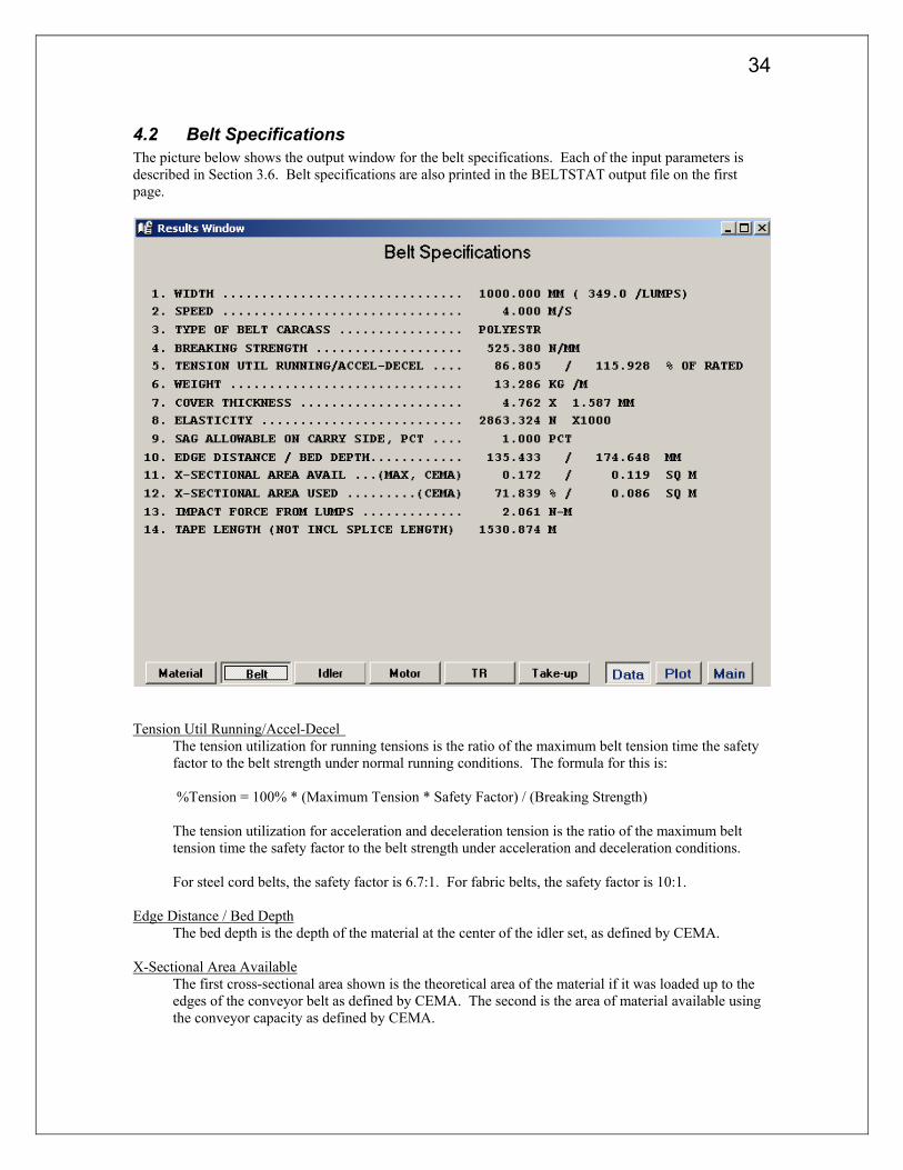
4.2 Belt Specifications The picture below shows the output window for the belt specifications. Each of the input parameters is described in Section 3.6. Belt specifications are also printed in the BELTSTAT output file on the first page.
Tension Util Running/Accel-Decel
The tension utilization for running tensions is the ratio of the maximum belt tension time the safety factor to the belt strength under normal running conditions. The formula for this is: %Tension = 100% * (Maximum Tension * Safety Factor) / (Breaking Strength) The tension utilization for acceleration and deceleration tension is the ratio of the maximum belt tension time the safety factor to the belt strength under acceleration and deceleration conditions. For steel cord belts, the safety factor is 6.7:1. For fabric belts, the safety factor is 10:1.
Edge Distance / Bed Depth
The bed depth is the depth of the material at the center of the idler set, as defined by CEMA. X-Sectional Area Available
The first cross-sectional area shown is the theoretical area of the material if it was loaded up to the edges of the conveyor belt as defined by CEMA. The second is the area of material available using the conveyor capacity as defined by CEMA.

35
X-Sectional Area Used This cross-sectional area is that of the material for the case being analyzed. This is based on the design tonnage, the given bulk density, and the belt speed. The program also shows the cross-sectional loading percentage. This represents the area defined as 100 percent of CEMA.
Impact Force from Lumps
This represents the energy that a lump imparts to the conveyor belt at the loading station. This is computed from the lump size, bulk density, lump shape factor, and chute drop distance.
Tape Length (Not Incl. Splice Length)
Total length of the belt not including additional lengths created by the splices.

36
4.3 Idler and Ancillary Specifications The picture below shows the output window for the idler specifications. Each of the input parameters is described in Section 3.6. Belt specifications are also printed in the BELTSTAT output file on the first page.
Idler Name / Series See Section 3.7.4 Idler Angle See Section 3.7.1 / 3.7.2 Diameter See Section 3.7.5 Load Rating See Section 3.7.9 Adjusted Load Capacity
The program computes this according to the method outlined by CEMA. The idler load rating is adjusted by the following factors:
o Lump Adjustment Factor o Environmental and Maintenance Factor o Service Factor o Belt Speed Correction Factor Applied Load At Max Spacing
This is the maximum applied load on the idler sets in any of the flights of the conveyor. This load does not include belt tension loads in vertical convex curves.
Rotating Weight See Section 3.7.8 Seal Drag (Ai) See Section 3.7.6

37
Number Of Idlers This is an approximate count of the idlers sets required for the conveyor.
Number Of Rollers See Section 3.7.3 KXC , KXR Coulomb friction factor for the carry and return idlers. See section 3.7.7 (KY) Trough Shape Multiplier See Section 3.7.10 / 3.7.11 (KY/KX) Correction (Regeneration) See Section 3.7.13 (KT) Temperature Adjustment (KY/KX) See Section 3.7.12 Idler Seal Correction (Regeneration)
The idler seal correction factor is related to the KY and KX regenerative correction (See sections 3.7.13). The idler seal correction factor will be set to 1 if the Ky and KX regenerative correction is greater than or equal to 1, otherwise it will be equal to 0. For example for a regenerative conveyor the Kx/Ky factor would be set to 0.666. In this case the Idler Seal Drag is automatically set to 0 and the Idler Seal Correction output will be 0.
Skirtboard Friction Factor See Section 3.7.14 Skirtboard Width See Section 3.7.15 Max Mat. Height
This is the height of material in contact with the skirtboard walls, when traveling at full belt speed. It is used by the program to compute the friction of the material scraping on the skirtboard walls. If the belt cross- sectional loading is low, a value of zero may result, indicating that the material does not contact the skirtboards.

38
4.4 Motor / Reducer / Brake Specifications
Location Of Drive / Brake Units
Locations of each drive station in the conveyor. Motor Nameplate HP/KW See Section 3.8.1 Motor Running HP/KW
This indicates the power that the motor must output to maintain the conveyor at full speed. If negative, this indicates the regenerative energy that must be absorbed by the motor.
Power Ratio See Section 3.8.2 Motor Synchronous RPM See Section 3.8.3 Motor Running RPM
This shows the slip RPM of an induction motor at the indicated running horsepower. This is based on an assumed full load RPM at (100-Drive Slip)% of the synchronous RPM. For example, at 2% drive slip the full load RPM from a synchronous speed of 1800 RPM would be 1764 RPM. See also section 3.8.13.
Starting Torque Limit (Pct Fll-ld-tq) See Section 3.8.4 Drive Inertia at Motor See Section 3.8.5 Drive Efficiency See Section 3.8.6 Drive Wrap Angle
The wrap angle of the drive pulley as input in the element table. (See Section 3.9.14). Drive Friction Factor See Section 3.8.7 / 3.8.8

39
Gearbox Ratio The gearbox ratio is computed from the motor running RPM, the belt speed, and the drive pulley diameter.
Brake Torque Lowspeed
This represents the brake torque that is to be applied to the pulley shaft. Brake Energy Absorbed
This output variable indicates how much heat the brake must absorb during the stopping cycle from full speed to zero speed. A negative value indicates that the brake would have to produce power to obtain the desired stopping time.
Acceleration Time and Travel
The acceleration time shown is either the input or resulting time from the starting torque limit. The travel represents the amount of distance the belt moves during the starting cycle.
Drift Time and Travel
The drift time is the time it will take the conveyor to stop from full speed with no braking action. The travel is the distance the belt will move during this cycle. A negative drift time will result for regenerative conveyors and the absolute value represents the time it would take the conveyor to accelerate from zero to full speed with no driving or braking forces imposed upon it.
Braking Time and Travel
This is similar to the acceleration time and travel, but for the braking cycle.

40
4.5 TENSION SPECIFICATIONS and "Tension" Window The Tension specifications in the BELTSTAT output file and the "Tension" window in the user interface show similar information. The “Tension” window in the user interface combines information from the Flight Profile Summary and the Tension Specification in the output file.
Flight No.
Number of the flight. Station Item
This is a description of the flight. The possibilities for this column are: TAIL: Tail Station HEAD P: Head pulley HEAD DR#: Head pulley and drive combination DRIVE #: Drive TAIL DR#: Tail pulley and drive combination TAKE-UP: Take up TAIL TU: Tail pulley and take up combination BEND P: Bend pulley SKIRTBDS: Skirtboard LOAD/SKT: Load station with skirtboard LOAD STN: Load station CONCAV R: Vertical concave curve. CONVEX R: Vertical convex curve. Ground X &Length
Station and Length of the individual flight Ground Y & Height
Elevation & Height of the individual flight

41
Running Tension Tension at the flight under normal running conditions.
Empty Tension
Tension at the flight when the belt in empty of all material. Accelerating Tension
Tension in the belt during acceleration. Brake Tension
Tension in the belt during the braking cycle. Drift Tension
Tension in the belt during a drift cycle. Sag Tension
Indicates the minimum allowable running tension that will comply with the previously defined sag criteria. If the user does not specify the counterweight tension, the program selects one which will meet the sag tension requirements of all the flights on the conveyor for the running case.
Loading
The loading of the individual flight as a percentage of the actual conveyor "Loading" Flap Mode
The flap mode column indicates when the forced vibration of the belt in that flight coincides with the belt's natural frequency. This condition can result in dangerously large belt oscillations, or resonance, and should be avoided. If the belt vibrations are near resonance then this column will contain the mode of resonance. For example, a flap mode of 1.10 indicates that the belt is near the first resonance mode. The flap mode is a function of the belt velocity, tension in the belt, weight of the material, idler diameter, and the idler spacing. If the belt in a flight is near a flap mode it is advisable to change one of the above parameters in order avoid resonance of the belt. Four stars (****) mean that the belt is not near a resonance mode.
V-Curve Radius
Vertical curve radius as specified in the "Element" Table. If the radius was left blank in the "Element" Table the program will estimate an approximate radius.
H-Curve Radius
Horizontal radius as specified in the "Element" Table KY
This column indicates the KY values. See section 6.3.1 for the method of computation.

42
4.6 "Tension Ratio" – Drive / Brake Tension Ratios The picture below shows the output window of the Drive/Brake Tension Ratios.
The same information is found in the BELTSTAT output file after the flight tension table. Below is an example of the TE and tension ratio summary in the BELTSTAT output.
TE
This shows the effective tension at each drive station for each tension case. This is simply the difference of the incoming and outgoing tensions, minus any gravity and/or acceleration/ deceleration forces active between these two flights.
WR Factr
This window shows the tension ratios for the running, acceleration, and braking cases. The warp angle, static coefficient of friction, and dynamics coefficient of friction are also shown.

43
For each load case two values are shown. The first is the wrap factor. The wrap factor is the maximum allowable tension ratio of the drive pulley before belt slip on the pulley will occur. The wrap factor is calculated from the following formula.
θfe Factr WR = Where:
WR Factr = Wrap factor e = natural logarithm (2.71828) θ = Wrap angle of the given drive pulley (radians) f = Friction factor of the given drive
For the running case the static coefficient of friction is used, whereas for the acceleration and braking cases the dynamic coefficient of friction is used. The wrap factor is used to evaluate whether the drive pulley has adequate slack side tension to avoid slippage. The wrap factor is shown for each tension cases because the friction factor varies between the running case and the other tension cases.
T1/T2 This value is the ratio between the greater and lesser of the tensions entering and leaving a drive station. The values are shown for all drive stations on the conveyor. The T1/T2 ratios should be compared with the corresponding wrap factor. If the T1/T2 ratio is less than the corresponding wrap factor, the slip criteria have been met.
If the slip criteria are not met, the user must modify the design by increasing the counterweight tension, increasing the acceleration or braking time, etc. The program should then be re-executed.
4.7 "Take-up" Specifications General Discussion about Take-up Tension and Displacement Take-up Datum Position
The take-up travel in BELTSTAT assumes a zero baseline or datum position for an initially applied take-up force and typical installation slack. The datum is not reference to any physical item such as a pulley. Input take-up tension, belt mass and elasticity, idler spacing, and conveyor geometry affect the datum position. If these variables do not change, then the take-up position from various BELTSTAT runs may be directly compared. However, if any of the above variables change then the take-up datum position also changes. Input take-up tension and actual take-up tension will be the same for a gravity take-up. However for a fixed take-up, input take-up tension and actual take-up tension can (and usually) will be the different. For example, if all variables remain the same on a gravity take-up system except for take-up tension then the take-up travel from the two runs are not relative to one another. BELTSTAT will show that the tension travel of the empty belt of both cases is approximately the same. Obviously, the belt stretch of the case with the higher take-up tension is the greatest. The take-up pulley on a gravity take-up will generally be near the datum position when the belt is empty at 20 C. However, the absolute take-up displacement is not important, only the relative position is important.

44
Take-up travel direction
Increasing positive take-up displacement indicates stretching in the belt. Therefore in a vertical gravity take-up, positive displacement means the take-up pulley moves downward.
Gravity Take-up
A gravity take-up has constant belt line tensions and variable displacement. The input take-up extension (in the Drives window) is not meaningful for a gravity take-up.
Fixed Take-up
A fixed take-up is a conveyor belt tensioning device that does not allow movement of the take-up pulley. Consequently, the belt tension at the take-up pulley varies during different loading or starting and stopping conditions. Belt mass must be input for a fixed take-up.
Explanation of Output Variables Take Up Flight and Type
This is the location and type of the take up. Input Take-up Tension
The take-up tension input by the user. Input Displacement
This is the input displacement of the take up. This field is only meaningful for a fixed take-up. Output Tension
The tension values calculated and used by BELTSTAT. Take-up Tension Differential
This value represents the change in the counterweight tension that would just satisfy the friction criteria for all drive pulleys for all tension cases. The friction criterion is determined by the minimum allowable coefficient of friction between the drive pulley and belt and the drive wrap angle. The friction criterion sets the minimum belt tension to prevent belt slip on the drive. Thus, if the counterweight tension is too low to satisfy the friction criteria, the designer may choose to increase it by the amount shown and re-execute the program. If the value shown is negative, this indicates that the counterweight tension can be reduced and still meet the friction criteria. The computation of this value does not consider sag criteria, which also must be met, and which may govern the setting of the counterweight tension.
Governing Case
This field shows which case govern the Take-up differential. Take-up Tension Differential SAG
This value represents the change in the counterweight tension that would just satisfy the belt SAG criteria.
Load Case Summary
Figure 1 shows the take-up force and displacement summary in the user interface. For this particular conveyor, the take-up pulley will be 30 mm from the datum when empty and 370 mm from the datum when fully loaded. Maximum displacements occur during acceleration and braking. The total take-up range is 510 mm. Figure 3 shows the relative position of the take-up pulley for various load cases.

45
Figure 1 Take-up Summary
In the BELTSTAT output file, the take-up summary (labeled “COUNTERWEIGHT SPECIFICATIONS”) is located after the drive tension differential summary and before the profile summary. Figure 2 shows the take-up summary in the output file. The tension travel summary is the fourth line in the left-hand box. It also shows the location of the take-up displacements for each load case.
COUNTERWEIGHT SPECIFICATIONS ( DIMENSIONS IN METERS ): TAKEUP TENSION ............... 48000. N LENGTH OF SPLICE 1.62 THERMAL TRAVEL 0.24 TAKEUP TENSION DIFFERENTIAL .. -18152. N PERM. ELONGATION 1.02 (0.15 %) TAKEUP DISPL. 3.0 GOVERNED BY DRIVE NO. 2, RUNNING CASE TENSION TRAVEL 0.370 0.025 0.447 -0.059 0.059 TAKEUP PT. ( 11) GRAVITY INPUT DISPL. 0.371 INPUT TAKEUP TENSION ......... 48000. N
running
empty
accel.
brake drift Figure 2 Take-up Summary in output file
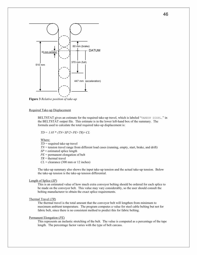
46
DATUM60 mm (brake)
447 mm (acceleration)
510 mm
30 mm (empty)
370 mm (full)
Figure 3 Relative position of take-up Required Take-up Displacement
BELTSTAT gives an estimate for the required take-up travel, which is labeled “TAKEUP DISPL.” in the BELTSTAT output file. This estimate is in the lower left-hand box of the summary. The formula used to calculate the total required take-up displacement is:
TD = 1.05 * (TN+SP/2+PE+TR)+CL Where: TD = required take-up travel TN = tension travel range from different load cases (running, empty, start, brake, and drift) SP = estimated splice length PE = permanent elongation of belt TR = thermal travel CL = clearance (300 mm or 12 inches)
The take-up summary also shows the input take-up tension and the actual take-up tension. Below the take-up tension is the take-up tension differential.
Length of Splice (SP)
This is an estimated value of how much extra conveyor belting should be ordered for each splice to be made on the conveyor belt. This value may vary considerably, so the user should consult the belting manufacturer to obtain the exact splice requirements.
Thermal Travel (TR)
The thermal travel is the total amount that the conveyor belt will lengthen from minimum to maximum ambient temperature. The program computes a value for steel cable belting but not for fabric belt, since there is no consistent method to predict this for fabric belting.
Permanent Elongation (PE)
This represents an inelastic stretching of the belt. The value is computed as a percentage of the tape length. The percentage factor varies with the type of belt carcass.

47
Tension Travel (TN) This is the total length that the belt will stretch compared to the state at rest, when the conveyor is not running. The computation of these values considers the elastic stretch and sag between idlers along each flight of the conveyor. The tension travel is shown for the running, empty, acceleration, brake, and drift tensions.
4.8 Force / Drag Summary This output is found at the end of the BELTSTAT *.BSO file.
Drive Pulley Drag
These are the drag tensions induced by the pulley bearings at each drive pulley. These drag forces are separated by the program from other drag forces because these drag losses, like gear reducer losses, are not driven through the drive pulley / belt interface.
Lift Force
This represents the net gravity force acting on the conveyor belt. If the flight heights sum to zero, the lift force equals the force required to lift the conveyed material. Since the lift force is the same for all tension cases (running, acceleration, braking, and drift), only one value is shown.
Friction Force
This represents the sum of all frictional forces excluding miscellaneous drag forces. This friction force applies to the running, acceleration, braking and drift tension cases.
Total Miscellaneous Force
This is the sum of all miscellaneous drag forces. Like the friction force, this value applies to the running, acceleration, braking and drift tension cases.
4.9 Conveyor Summary This output is found at the end of the BELTSTAT *.BSO file.
Horizontal Length
Here the program shows the arithmetic sum of all straight-line flight lengths. This value does not include any allowance for extra belt length needed to splice the belt.
Total Elevation
The total elevation change in the conveyor from the tail to the head of the conveyor. Material Lift
The total height that the material must be raised. Sum of Flight Heights
This is the sum of height of each flight (carry and return). It should sum to zero. Total Mass
This is the sum of all the individual flight masses.
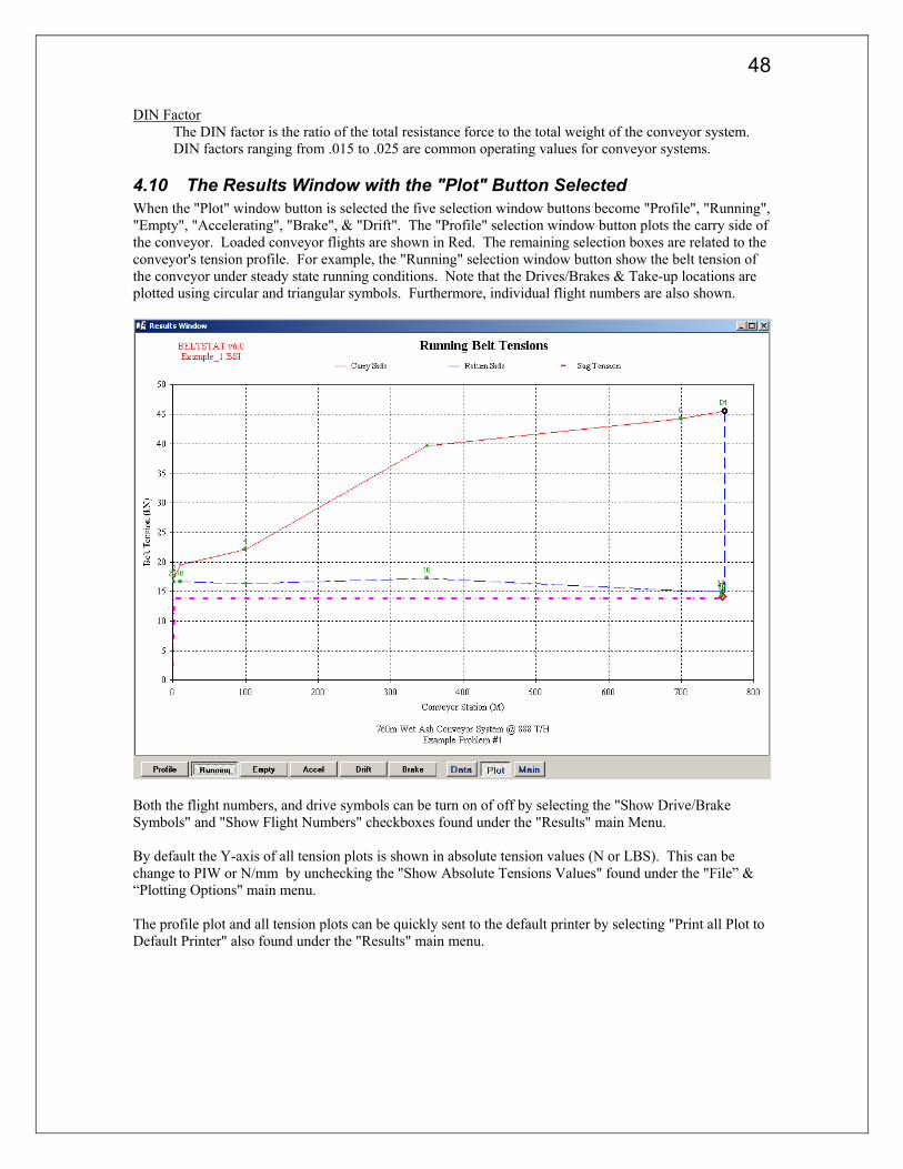
48
DIN Factor The DIN factor is the ratio of the total resistance force to the total weight of the conveyor system. DIN factors ranging from .015 to .025 are common operating values for conveyor systems.
4.10 The Results Window with the "Plot" Button Selected When the "Plot" window button is selected the five selection window buttons become "Profile", "Running", "Empty", "Accelerating", "Brake", & "Drift". The "Profile" selection window button plots the carry side of the conveyor. Loaded conveyor flights are shown in Red. The remaining selection boxes are related to the conveyor's tension profile. For example, the "Running" selection window button show the belt tension of the conveyor under steady state running conditions. Note that the Drives/Brakes & Take-up locations are plotted using circular and triangular symbols. Furthermore, individual flight numbers are also shown.
Both the flight numbers, and drive symbols can be turn on of off by selecting the "Show Drive/Brake Symbols" and "Show Flight Numbers" checkboxes found under the "Results" main Menu. By default the Y-axis of all tension plots is shown in absolute tension values (N or LBS). This can be change to PIW or N/mm by unchecking the "Show Absolute Tensions Values" found under the "File” & “Plotting Options" main menu. The profile plot and all tension plots can be quickly sent to the default printer by selecting "Print all Plot to Default Printer" also found under the "Results" main menu.

49
4.11 The Results Window with the "Main" Button Selected When the "Main" window button is selected the five selection window buttons become "Summary", "Tension", "Concave", "Convex", "Loss Table", & "" (blank, for future use). Many of the variables will be highlight in "RED" if they are above acceptable or below certain levels. For example, if the calculated drive tension ratio is greater than the acceptable tension ratio (calculated by the drive wrap angle and friction factor given in the user input) the value will be highlighted in red.
4.11.1 "Summary" Window Selection Button The "Summary" window is set as the default window when viewing the BELTSTAT results. Although this data is also found in other locations, its purpose is to act as a "quick" information window showing some of the most critical and frequently referenced data in a single location.
4.11.2 "Tension" Window Selection Button See Section 4.6

50
4.11.3 "Concave" Window Selection Buttons
Here the program gives a detailed analysis of the curve radii shown previously. This analysis is done for both the carry side and return side of the conveyor, but is not done at any flight where a pulley exists. This information will not be printed in the output file unless the " Output Curve Report "checkbox is checked. Maximum Allowable Center Tension
The program uses an allowable value equal to the belt rating for the running tension case. It uses a forty percent overstress as the allowable value for temporary tension cases.
Flight Number
The flight of the curve. Selected Radius
The radius at the flight. Tension Case
Indicates what the tension case is for the particular row. Minimum Allowable Edge Tension
For fabric belting, 30 PIW is used. For steel cable belting, the CEMA criteria is used. This criteria calls for setting the radius using 30 PIW as the minimum stress and then dividing that radius by 2.5. This results in a much lower allowable edge tension (usually negative).

51
Edge and Center Tensions Here the theoretical stress at the edges and center of the belt are shown. These are computed from the belt tension at the curve, the curve radius, belt elastic modulus, belt width, trough shape, and idler angle.
Lift Radius
The program computes the radius at which belt lift would be impending, using the computed tensions at the given flight. The lift radius is computed using the weight of the belt plus that of the material on it. The lift radius is also computed using the weight of an empty belt, though the same belt tension is used.
4.11.4 "Convex" Window Selection Buttons
Minimum Allowable Center Tension
This is the minimum tension at the center of the belt Maximum Allowable Edge Tension Idler Vertical Tolerance
This is the vertical tolerance which the installed idlers can have for the given calculations. Idler Corrected Load Capacity
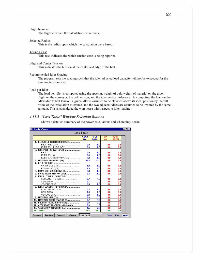
52
Flight Number
The flight at which the calculations were made. Selected Radius
This is the radius upon which the calculation were based. Tension Case
This row indicates the which tension case is being reported. Edge and Center Tension
This indicates the tension at the center and edge of the belt. Recommended Idler Spacing
The program sets the spacing such that the idler adjusted load capacity will not be exceeded for the running tension case.
Load per Idler
The load per idler is computed using the spacing, weight of belt, weight of material on the given flight on the conveyor, the belt tension, and the idler vertical tolerance. In computing the load on the idlers due to belt tension, a given idler is assumed to be elevated above its ideal position by the full value of the installation tolerance, and the two adjacent idlers are assumed to be lowered by the same amount. This is considered the worst case with respect to idler loading.
4.11.5 "Loss Table" Window Selection Buttons Shows a detailed summary of the power calculations and where they occur.

53
4.12 View BSO File This window show the actual BELTSTAT output file (*.BSO file). This window contains the same information shown the standard Results Window. It is identical to the "View" command in BELTSTAT v5.0. This file is saved a DOS text file so it can be easily E-mailed to clients or other engineers. The text file can be printed by non BELTSTAT users by using the DOS “EDIT” command.
Number Keys (1,2,3,4) These keys will jump to a specific output page (i.e. Page 1, Page 2, etc.). Arrow Keys / Page Up / Page Down The arrow and Page keys move the user around the output window. End Key Quickly moves the user the end of the file Home Key Move the users to the beginning of the file. Esc Key Closes the output window

54
5.0 PROFESSIONAL VERSION FEATURES The following features are only available in the professional version of BELTSTAT.
5.1 Project Files The "Project Files" is activated by either clicking the "Project" toolbar button or by selecting the "Project Files" option submenu found under the "Professional" heading in the main menu. This feature allows the user to quickly and easily determine the "worst cases" scenarios for a particular conveyor system. The user begins with a single input file. This "Master" file represents the conveyor system in its normal operational state. By pressing the "Create Project Files" button six new input files are generated base on the "Input Table". Each new input file represents a "worst case" or "unique" operating state of the "Master" conveyor system. By selecting the "Run Project Files" all seven files (1 maser file and the 6 newly created files) are ran with their individual results appearing in the "Results" window.

55
5.1.1 Project Files - Input Table A sample table has been included with the program. THIS TABLE IS ONLY A SAMPLE INPUT TABLE. Its values should NOT be used as absolute or universal values only sample values. Each and every conveyor is unique, and individual design parameters will vary depending on the design specifications. Therefore each input table should be modified for each conveyor design. When a "Project File" is saved the values in the "input Table" are also saved to the project file. Therefore, the user can easily change these values for each project, and they will automatically be recalled when reopening the project. The "Input Table" values can also be save to the BELTSTA.INI file by selecting "Make Current Input Values the Defaults" under the "Professional" main menu. This sets the current values in the input file as the universal program defaults. Any variables left blank will default to the value in the "Maser File". File Name Addition
This is the extension that will be added to the current file name. For example, if the "Master File" is called "C1-R3.bsi" and the file extension is "-FW" (abbreviation for the Full Winter Case) the new file name will be C1-R3-FW.bsi". Note: The “-FN” extension (full normal condition) is a special extension. If the master filename is “C1-FN.bsi” then all the project files will be created WITHOUT the “-FN” extension. In general the master file should always be name with the “-FN” extension. For example “C1-R3-FN” for the master file and then all the project files would be named “C1-R3-XX”.
Conveyor Description See "Conveyor Description"
A new description for the individual file. General Remarks See "General Remarks"
These remarks will be ADDED to the current "General Remarks" of the "Master File". Design Tonnage See "Design Tonnage"
This value will replace the "Design Tonnage" value in the "Master File" Loading Multiplier See "Loading Multiplier"
This value will replace the "Loading Multiplier" value in the "Master File" Minimum Temperature See "Minimum Temperature"
This value will replace the "Minimum Temperature" value in the "Master File" Maximum Temperature See "Maximum Temperature"
This value will replace the "Maximum Temperature" value in the "Master File" Belt Loading ("",C,N,I,D,#)
This will reset the conveyor loading for the file based on the following inputs. Blank - No Change C - Load the Carry Side N - Unload All Flights I - Load Inclines D - Load Declines
# - Load Specific Flight Numbers (ex. "#23-34" will Load flights 23 to 34)
56
Skirtboard Loading (*) See "Conveyor Loading" This value (0-1) will be multiplied by the current Skirtboard Loading (flights in the element table that have an ID type of "S") flights in the "Master File".
Belt Weight (*) See "Belt Weight"
This is a multiplication factor to increase (or decrease) the belt weight. The design may want to increase the belt weight (10-15%) to compensate for possible "manufacturing" tolerances in the belt. For an inclined conveyor system this may represent a design parameter for the Maximum Power consumed (or Maximum regeneration for a decline system). On the other hand the designer may want to decrease the belt weight slightly thereby assuming a lower than expected belt weight or determine the effect of possible weight loss do to belt wear.
Top & Bottom Cover Thickness (+) See "Top Cover Thickness"
As opposed to changing the actual belt weight (above) the top & bottom cover thickness may be specified in the "Master File". If so the values entered in "Top Cover Thickness (+)" and "Bottom Cover Thickness (+)" will be added (or subtracted) from the "Master Files" value and the program will calculate a new belt weight.
Seal Friction - Carry (*) & Return (*) See "Seal Friction"
This multiplication factor will cause the seal friction to be increases or decreased. It is important to remember that the seal drag is only relevant when using user-defined idlers. If standard idlers sets, "C6" for example, are used in the "Master File" then the seal friction is irrelevant.
Trough Shape Mult - Carry & Return See "Trough Shape Multiplier"
A specific Trough Shape Multiplier may be entered. Kx / Ky Correction See "Kx / Ky Correction"
A specific Kx / Ky Correction factor may be entered. Starting Torque Limit See "Starting Torque Limit"
The Starting Torque limit for ALL drives may be specified. Drive Efficiency See "Drive Efficiency"
The Drive Efficiency for ALL drives be specified. Friction Factor - Running See "Drive Friction Factor - Running"
A Friction Factor for ALL Drives may be specified. Friction Factor - Accelerating See "Drive Friction Factor - Accelerating"
A Friction Factor for ALL Drives may be specified. Acceleration Time See "Acceleration Time"
The Acceleration Time for ALL Drives may be specified. Brake Time See "Brake Time"
The Brake Time for ALL Drives may be specified. Brake Torque See "Brake Torque"
The Brake Torque may be specified. Take-up Tension
The take-up tension for each case

57
Gearbox Ratio / Pulley Diam This is used to allow the user to specify a specific gearbox ratio rather than a belt speed. In real life the motor RPM will vary as a function of power, and therefore belt loading. In most cases an empty conveyor will actually have a slightly higher belt velocity than a fully loaded conveyor. By entering the gearbox ratio and pulley diameter, BELTSTAT will adjust the belt velocity for each load case to achieve the specified gearbox ratio. This is an iterative process and in most cases the project files will need to be re-run two to three times for the belt velocity and gearbox ratio to converge.
Number of Project Files
For some conveyors there may be additional cases that the design may want to create. For instance, a conveyor may have two steep incline sections and the designer may want to analize each incline section separately from the case when both are loaded. Up to 15 unique case files can be created and saved for each project.
Project Comments
This field is used one the project file printouts. Update Profile
In some cases the user may want to manually edit the conveyor loading once the project files have been created. If “Y” is entered in this box then the conveyor profile is not modified when the project files are updated.

58
5.1.2 Project Files - Results Table The "Results" window shows a quick summary of the results for each of the standard files ran. Specific information can be obtained by selecting the desired file (under the "Opened Files" main menu) and viewing the results as usual ("Results Window" or "View BSO File"). The results table can be printed by selecting the ”Print” button on the toolbar.

59
5.1.3 Project Files - Tension Table The "Tension" window shows a quick summary of the tension results for each of the standard files ran. This table list the maximum and minimum tensions found in ALL files.

60
5.2 Vertical Curve and Idler Calculations Before diving into the BELTSTAT input/output routines the engineer must first understand how to properly design a convex/concave curve and what information is relevant. Concave Curves Concave curve are generally governed by three criteria:
1. Belt lift off 2. Edge stress 3. Center stress.
The belt should not lift off a concave curve at the maximum belt tension when the belt local section is empty. What does this mean? It means that the designer should not only look at the fully loaded and empty belt tensions but at ALL possible design load cases and determine the maximum belt tensions in EACH flight. Furthermore, the curve radius should be large enough to prevent belt lift off when the belt weight has been reduced from its original weight to account for wear. For concave curves, the maximum stress occurs at the center line of the belt. CEMA specifies that the maximum allowable center stress should not exceed 115% of the nominal belt rating. A concave curve will cause the belt to buckle at the edge of the belt if the radius is too small. However, a certain amount of compressive stress is allowable at the edges for steel cord belts. Experience has shown that the compressive stresses on the edge cables do not damage the belt or the splice. The allowable compressive stress on the edge cables is tension dependent. Higher belt tension may have higher compressive stresses. The edge stresses must not fall below the allowable edge compressive stress. Convex Curves The radius of the vertical convex curve are governed by the following criteria:
1. Belt edge stress 2. Center stress 3. Idler spacing 4. Idler installation tolerances 5. Idler L10 hour rating.
For convex curves, the maximum stress occurs at the edge of the belt. CEMA recommends that the maximum allowable edge stress does not exceed 115% of the nominal belt rating. A convex curve will cause the belt to buckle at the center of the belt if the radius is too small. The stresses in the center of the belt should not drop below 5 N/mm during running conditions and 2.5 N/mm during starting and stopping. Curve Analysis Input Data The figure below shows the “general’ input window. The “Use project tensions from all opened files” box is very useful when working with conveyor projects. When this box is checked the belt tensions for all currently opens files will be used. Therefore, if you are working with a project that has the seven standard design files (Incline loads, declines loaded, high friction, low friction, etc.) BELTSTAT will get the maximum and minimum belt tensions from ALL files. If this box is uncheck BELTSTAT will only use the tensions from the current file.

61
The “Curve Data” input window mainly contains information regarding the belt safety factors. The minimum allowable belt stresses for both the steady state running and dynamic (starting/stopping) conditions are shown. Additionally the belt safety factor is also input. The “Max Edge/Center Stress” input box represents the maximum allowable belt stress at the center or edge of the belt. For example if the designer is using a belt safety factor of 6.67:1 and a maximum allowable edge stress of 115% then the safety factor at the belt edges would be 5.8:1 (6.67 / 1.15). CEMA allows a maximum edge/center stress of 115% of the nominal belt stress. This is the default value.
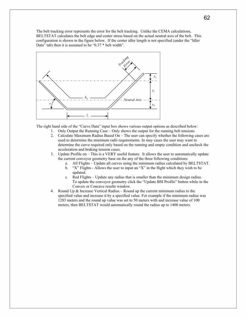
62
The belt tracking error represents the error for the belt tracking. Unlike the CEMA calculations, BELTSTAT calculates the belt edge and center stress based on the actual neutral axis of the belt. This configuration is shown in the figure below. If the center idler length is not specified (under the “Idler Data” tab) then it is assumed to be “0.37 * belt width”.
bw
lc
θNeutral Axis
yt
yb
ye
Trackin
g Erro
r
The right hand side of the “Curve Data” input box shows various output options as described below:
1. Only Output the Running Case – Only shows the output for the running belt tensions 2. Calculate Maximum Radius Based On – The user can specify whether the following cases are
used to determine the minimum radii requirements. In may cases the user may want to determine the curve required only based on the running and empty condition and uncheck the acceleration and braking tension cases.
3. Update Profile on – This is a VERY useful feature. It allows the user to automatically update the current conveyor geometry base on the any of the three following conditions:
a. All Flights – Update all curves using the minimum radius calculated by BELTSTAT. b. “X” Flights - Allows the user to input an “X” in the flight which they wish to be
updated. c. Red Flights – Update any radius that is smaller than the minimum design radius.
To update the conveyor geometry click the “Update BSI Profile” button while in the Convex or Concave results window.
4. Round Up & Increase Vertical Radius – Round up the current minimum radius to the specified value and increase it by a specified value. For example if the minimum radius was 1283 meters and the round up value was set to 50 meters with and increase value of 100 meters, then BELTSTAT would automatically round the radius up to 1400 meters.

63
The “Idler data” input tab contains information relevant to both the idler life calculations, and convex curve calculations. The troughing angle and center roll width are used to calculate the neutral axis of the belt. The other critical input is the “Adjusted Idler Load Rating” which will is automatically calculated when the user selects an appropriate idler series. The idler tolerance is also used to calculate the idler loading in the vertical curve analysis.
There are two analysis methods for idler calculations. The first is the CEMA method. This is the default methodology and is based off the standard CEMA idler sets and ratings. To us this method the designers simply select the appropriate idler series and environmental conditions. BELTSTAT will automatically calculate the correct “Adjusted Idler Load Rating” based on this input. The other calculation methodology is the “Advanced” methodology. When this method is selected two additional tabs (“Load Rating” and “Bearing Summary”) will appear at the top of the form. This method allows the user to select a specific bearing type, such as a 6308 bearing. Rather than using an “adjusted idler load capacity” the advance method uses a bearing static and dynamic load capacity. It then calculates the loading on each bearing according the information input in the “Load Rating” page. The advanced idler calculations are based off the original pressimeca calculations and the designer should refer to the original paper entitles “” for more complete information on this method.
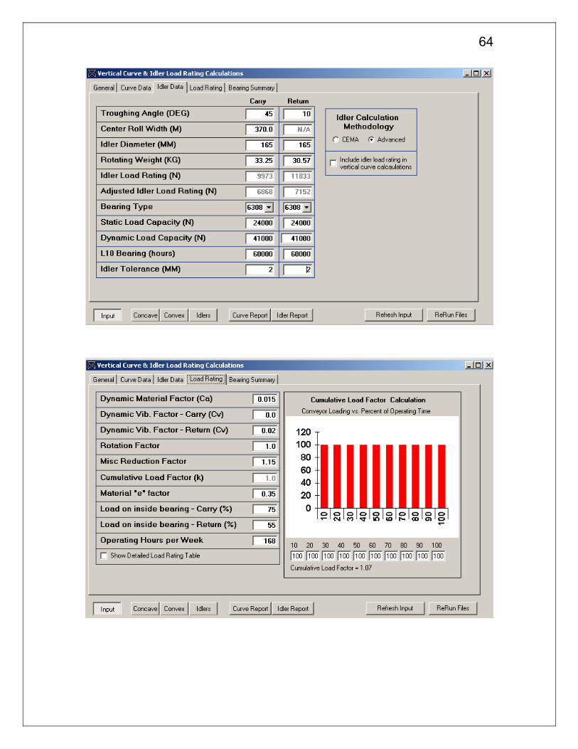
64

65
CONCAVE CURVE OUTPUT The figure below shows the output from a typical analysis.
1. Flight Number / Abs X/Y – This is simply the conveyor flight number and its absolute X and Y position along the conveyor. The X/Y information is useful when writing reports (“100 m Convex Curve at 140meters from the tail” for example).
2. Current & Required Radius – Show the Current radius (as specified in the element input table) and the required radius. The required radius will be selected as the maximum radius base in the “Calculate Maximum Radius Based On” checkboxes selecting in the “Curve Data” input window.
3. Minimum Required Radius – The minimum required radius for each load case. This is the MAXIMUM radius for columns 11-14.
4. Tension Case – The loading case 5. Minimum tension – The minimum belt tension for the flight. These values will be the same as the
maximum tension if “Use Project Tensions from all Opened Files” checkbox was unchecked in the “General” input tab (since there is only one file).
6. Maximum Tension – The maximum belt tension for the flight. These values will be the same as the minimum tension if “Use Project Tensions from all Opened Files” checkbox was unchecked in the “General” input tab (since there is only one file).
7. Minimum Allowable Edge Stress – This is the minimum allowable edge stress. 8. Edge Stress – This is the actual edge stress and must be greater than the minimum allowable edge
stress or the radii will need to be increased. 9. Center Stress – This is the center stress of the belt. For a concave curve this will be the highest
stress in the belt at that particular location (assuming no horizontal curve is present) 10. Safety Factor – The minim belt safety factor. 11. Radius – These columns show the minimum required radius for each condition. This allows the
user to quickly pinpoint the reason for a selected minim radius.

66
CONVEX CURVE OUTPUT The figure on the next page shows the output from a typical analysis.
1. Flight Number / Abs X/Y – This is simply the conveyor flight number and its absolute X and Y position along the conveyor. The X/Y information is useful when writing reports (“100 m Convex Curve at 140meters from the tail” for example).
2. Current & Required Radius – Show the Current radius (as specified in the element input table) and the required radius. The required radius will be selected as the maximum radius base in the “Calculate Maximum Radius Based On” checkboxes selecting in the “Curve Data” input window.
3. Minimum Required Radius – The minimum required radius for each load case. This is the MAXIMUM radius for columns 10-12.
4. Tension Case – The loading case 5. Minimum tension – The minimum belt tension for the flight. These values will be the same as the
maximum tension if “Use Project Tensions from all Opened Files” checkbox was unchecked in the “General” input tab (since there is only one file).
6. Maximum Tension – The maximum belt tension for the flight. These values will be the same as the minimum tension if “Use Project Tensions from all Opened Files” checkbox was unchecked in the “General” input tab (since there is only one file).
7. Edge stress – This is the edge stress in the belt. This is the maximum stress location in a convex curve.
8. Safety Factor – The belt safety factor at the above edge stress. 9. Center Stress – This is the center stress of the belt. For a convex curve this is the lowest stress
point in the belt. This stress must be greater than the minimum allowable belt stress. 10. Radius – These columns show the minimum required radius for each condition. This allows the
user to quickly pinpoint the reason for a selected minim radius. IDLER INFORMTION 11. Radius – This is the required radius for the current idler loading. In other words if the idler spacing
remains unchanged, then this would be the required radius to match the current idler load rating. 12. Current Idler Spacing – The current spacing of the flight 13. Maximum Idler Spacing – If the idler load rating and vertical curve were unchanged, then this is
the maximum spacing allowable. 14. Current idler load rating – The idler loading rating for the current vertical radii and idler spacing. 15. Spacing for minimum idler loading – This shows the idler spacing that would give the minimum
idler load rating. If the idler vertical tolerance is set to zero (in the input page), then as the spacing is decrease the idler loading will approach zero. However, if the idler vertical tolerance is not zero (say 2mm for example) then as the spacing is decrease the idler loading will actually increase at some point. This is because, although the material loading goes to zero, the normal force due to the idler vertical tolerance will become great as the spacing is reduce.
16. Minimum Idler load – This is the minim idler loading possible for the current vertical radius and idler spacing.

67

68
5.2 Belt Flap The Belt Flap window allows the user to easily determine if belt flap may be a problem in a specified tension range. This model is based on a simple string vibration model. The user should avoid resonate frequencies between 0.85 and 1.15 times a resonance frequency. A results table is also available and can easily be printed out by clicking the “print” button on the main menu.

69
5.3 Splice Pattern The splice window is only available in the Profession Version of BELTSTAT. All parameter for this window must be input in metric units. There are two input columns for this window. The first input column contains the data used by the program to "Automatically" calculate a 1, 2, 3, and 4 Step Splice. Using the parameters in the first column the program will determine the optimum Cable Diameter, Number of Cables, and other important parameters for each splice step. If these parameters can not be determined the program will output "0" in all the Splice Results output columns. The second column in the Splice window is the "Variables for the Select and Plot Splice". If the "Update Selected Splice on Recalculate" checkbox is check then the program will automatically fill in the value for the optimum splice pattern this column. However if the "Update Selected Splice on Recalculate" checkbox is unchecked then the user can enter any values desired in this column. All 1, 2, 3, and 4 Step splice configurations are supported.
Variables for the 1, 2, 3, 4 Step Splices Belt Width
The width of the conveyor belt. This value defaults to the currently select belt width. Maximum Belt Tension
The maximum belt tension at any flight along the conveyor system Safety Factor
This value defaults to 6.7. It is used to calculate the Target ST Rating. This is the ST rating the program is trying to solve for. This value differs for the "Actual" ST-Rating of the belt because of the following reasons:
The Number of cables in the Belt must be an integer Number The Number of Cables in the Belt Depends on the Splice Type (1 Step, 2 Step...) In General Cables are only available in specific sizes (3.1, or 3.2 mm not 3.135 mm)
The following equations are used to calculate the ST-Rating Target ST Rating = (Maximum Belt Tension * Safety Factor) / (Belt Width) Actual ST-Rating = (Number of Cables * Cable Breaking Strength) / (Belt Width)

70
Belt Edge Distance
The "unused" distance from the edge of the Belt to the first cable in the Splice region. (Default value of 25 mm)
Cable Strength Constant
This value is used to calculate the breaking strength of the cables as follows:
Cable Breaking Strength = (Cable Diameter)^2 * Cable Strength Constant
The default value is 875 but this value may be changed if the cables are stronger or weaker. Target G/D Ratio
If a specific G/D ratio is desired it can be entered here. The program will then use this value to try and determine the optimum cable parameters.
Update Selected Splice on Recalculate
If this box is checked then the Right-hand column of variables (Variables for the Selected and Plot Splice) are automatically updated.
Recalculate
Recalculates all variables Variables for the Select and Plot Splice Splice Type
All Splice type 1-4 step are support. Simply select the Splice pattern you desire. Number of Cables
Total number of cables in the parent belt. In order to have an optimized & symmetric splice pattern for a specific splice type this number must be as follows:
"1-Step Splice - 2N" "2-Step Splice - 4N" " 1-2-3 Splice - 6N" " 2-1-3 Splice - 6N" " 1-3-2 Splice - 6N+4" "1-2-3-4 Splice - 8N" "3-2-1-4 Splice - 8N" "3-1-4-2 Splice - 8N+4" "1-3-4-2 Splice - 8N+4" (where N is an integer greater than 2) Cable Diameter
Diameter of cable to be used in the belt. Cable Breaking Strength
Actual Breaking Strength of the Cable. If this value is unknown it can be estimated be the following formula.
Cable Breaking Strength = (Cable Diameter)^2 * Cable Strength Constant
Belt Width The width of the conveyor belt.

71
Belt Edge Distance
The "unused" distance from the edge of the Belt to the first cable in the Splice region. (Default value of 25 mm)
Splice Step Length
Individual length of a step. Splice Bend Zone Length of the "Bend Zone" of the Splice Butt Gap between Cables
End gap between cables in the splice region. Splice Pattern Results The results window contains three output windows. The first “Results” shows a summary of the current splice run. The second “Plot” shows a graphical picture of the current splice design. The third, “Report”, is a general report with all relevant information regarding the current splice.
Target ST Rating
ST Rating of the Belt - See "Safety Factor" above. Number of Cables
Number of cables in the parent Belt Cable Diameter
Diameter of the Cables Cable Breaking Strength
Breaking Strength of the Cables Pitch in Parent Belt
The pitch is defined as the distance between the centers of two cables in the parent belt (outside the splice region).
Cable Gap in Splice Zone
This is the Actually Gap between cable in the splice Region G/D Ratio
This is the Gap / Cable Diameter. This is just a standard parameter used in the splice industry. Belt Width

72
The Width of the Belt Maximum Belt Force
The maximum force the parent belt can withstand (neglecting edge, and other nonlinear effects) It is simple the Cable Breaking Strength * Number of Cables
Edge Distance
The "unused" distance from the edge of the Belt to the first cable in the Splice region. (Default value of 25 mm)
Step Length
The Length on One individual Step. Bend Zone Length
The Length of the Bend Zone Cable But Gap
End gap between cables in the splice region. Total Splice Length
The Total Length of the Splice Active Rubber Shear Cells
This number is the number of "Active" Shear cells divided by the total Number of shear cells in a "unit" splice pattern. In general the higher this number is the more efficient the splice is.
Active Shear Cells per Cable
Assuming a LINEAR Splice Model this is the number of Active Shear Cells per Cable.

73
5.4 Belt Turnover Calculations The professional version of BELTSTAT includes an analysis program for belt turnovers. Classical turnover analysis determines the stresses based on the belt twist only and does not include the effects from:
1. belt sag 2. middle support rollers
Belt sag increases the edge stress at bottom edge and decreases the edge stress at the top edge of the belt. The change in stresses is due to bending of the belt. Stresses caused by belt sag can be significant and should not be ignored. Middle support rolls are often placed in turnovers to decrease the belt sag and also to decrease edge stresses caused from belt sag. The turnover analysis program in BELTSTAT includes the effects from belt twist, belt sag, and middle support rolls. Two different types of turnovers may be analyzed, which are flat helix turnover with support rolls and flat helix turnover without middle support rolls. Figure 1 shows a flat helix belt turnover without any middle support rolls. Figure 2 shows a flat helix belt turnover with middle support rolls.
Figure 1 – Flax helix turnover without middle support rolls
Figure 2 – Flat helix turnover with middle support rolls

74
CALCULATION METHOD Belt stresses in the turnover are resultants of the following items:
1. Belt tension (σTension) 2. Belt twist (σTwist) 3. Bending stresses in vertical plane (σSag) 4. Bending stresses in horizontal plane (only when the turnover has middle support rolls) (σHorizontal)
The following items describe the basic calculations methods:
1. Belt Tension Stress σTension = Tension / Belt width
2. Belt Twist Stress
Stresses from belt twist is calculated by assuming a 180 degree helix twist displacement and then calculating the corresponding stress. The edge and center stresses are:
+
⋅⋅
+−⋅
= 12
13
2 2
, LBWE
edgeTwistπσ
+
⋅⋅
+−−
= 12
13
2
, LBWE
centerTwistπσ
3. Bending Stresses in Vertical Plane
The belt sags in the turnover resulting in bending stresses. The bending stresses are a function of the curvature of the belt.
ZZ
ZSag I
yM ⋅=σ
The bending stress must be numerically calculated. Both the bending moment (MZ) and the moment of inertia (IZZ) are not linear. Also, the bending moment is different for turnovers with middle support rolls and those with out support rolls. The bending moment must be solved directly from differential equations. The moment of inertia is calculated as a function of the belt orientation along the length of the turnover. Figure 3 shows the force diagram in the vertical plane.

75
Figure 3 Force Diagram in Vertical Plane
4. Bending Stresses in Horizontal Plane
If the turnover has middle support rolls, there will be curvature in the horizontal plane as well as the vertical plane. The bending stresses are a function of the curvature of the belt.
YY
YHorizontal I
zM ⋅=σ
Again, the bending stress must be numerically calculated. Both the bending moment (MY) and the moment of inertia (IYY) are not linear. The bending moment must be solved directly from differential equations. The moment of inertia is calculated as a function of the turnover shape. If there are no middle support rollers then the horizontal stresses are zero.
Figure 4 Force diagram of belt turnover in horizontal plane
Figures 3 and 4 show that the middle support rolls apply a force in both the vertical and horizontal directions. In the vertical plane, the rolls apply an upward force on the belt and therefore reduce belt sag. However in the horizontal plane, the middle support rolls apply a force opposite to each other. The boundary conditions of the belt require that the horizontal displacement is zero at the ends of the turnover. The Horizontal B.C. Length (LHBC) is the location at which the displacement in the horizontal plane is forced to zero. This variable boundary condition length is included in the analysis to better simulate the real boundary conditions in the turnover. This length must be zero or greater. Increasing the length LHBC will decrease the horizontal bending stresses. In general, we recommend setting LHBC to two times the belt width.
Figure 5 shows both the horizontal and vertical displacements in a 36 m turnover with middle guide rolls. The length LHBC has been set to two meters in this turnover. The vertical displacements come to zero at x=0 and x=36 m (at the ends of the turnover). However, since LHBC is set to two, the horizontal displacements don’t come to zero until x=-2 and x=38 meters (two meters past the turnover ends).

76
-0.1
-0.08
-0.06
-0.04
-0.02
0
0.02
0.04
0.06
0.08
0.1
-2 0 2 4 6 8 10 12 14 16 18 20 22 24 26 28 30 32 34 36 38
Distance from Edge Roller (m)
VerticalHorizontal
Vertical and Horizontal Belt Displacement in Turnover
Middle Guide Rollers are included in analsyis
Figure 5 Sample displacement of 36 m belt turnover 5. Integration Step
Since bending moment and belt sag must be numerically determined, an integration step must be provided to the analysis program. A large integration step will calculate the stresses very quickly but will not be as accurate as a smaller integration step. We recommend using an integration step equal to the belt width.
INPUT PARAMETERS Figure 6 shows the belt turnover input box. Each parameter is explained below.

77
Figure 6 Belt Turnover Input Box The table below explains each input parameter.
1. Belt Width Belt width input
2. Breaking Strength Breaking strength input (N/mm) in metric, or belt rating (PIW) in Imperial units
3. Belt Weight Belt weight 4. Belt Elasticity Belt elasticity
5. Middle 45 Deg Guide Rollers If the turnover has middle guide rolls, then set to “YES” other wise set to “NO”
6. Horizontal B.C. Distance This parameter only applicable if Item 5 (Middle guide rolls) is set to “YES”. This is the distance LHBC as shown in Figure 4. The recommended value is twice the belt width.
7. Minimum Turnover Length This is the minimum belt turnover length you wish to analyze. 8. Maximum Turnover Length This is the maximum belt turnover length you wish to analyze.
9. Increment Step Length
This is the incremental belt turnover length you wish to analyze. For example, if min length = 10, max length = 20, and increment length = 2 then turnover lengths of 10, 12, 14, 16, 18, and 20 will be analyzed.
10. Integration Step Size This is the integration step for the numerical solver. The recommended step size is the belt width.
11. Running Tension 12. Empty Tension 13. Acceleration Tension 14. Braking Tension 15. Drift Tension
These are the tensions which will be analyzed in the turnover.

78
TURNOVER OUTPUT REPORT The output report shows the input parameters used in the calculations and the results of the analysis. The able below describes the turnover results.
Column Column Label Description
1 Length This length of the turnover
2 Center Twist This is the component stress at the neutral axis of the turnover caused by belt twist. This stress is negative.
3 Edge Twist This is the component stress at the edge of the belt of the turnover caused by belt twist.
4 Max Sag This is the maximum component stress caused by bending in the vertical plane (belt sag).
5 Max Horz This is the maximum component bending stress caused by the middle guide rolls in the horizontal plane.
6 Max Top
This is the maximum total edge stress along the top edge of the turnover. Note that the component stresses do not necessarily add up to the maximum edge stress since the maximum component stresses may be located at different locations.
7 Max Bottom This is the maximum total edge stress along the bottom edge of the turnover.
8 Min Stress
This is the minimum stress that occurs in the turnover. Since the twisting causes compressive stresses in the center of the belt and bending (both vertical and horizontal) causes negative stresses, it is possible to negative total stresses in the turnover. It is recommended, as in vertical convex curves, that stresses always be positive in belt turnovers.
9 Belt Safety Factor
This is the minimum belt safety factor as calculated with the maximum edge stress.
10 Sag This is the estimated sag of the belt in the turnover. 11 Percent sag This is the percent sag based on the total turnover length.

79
SAMPLE BELT TURNOVER PROBLEM Given: A conveyor is to be installed with a flat helix belt turnover. The following table shows the belt properties.
Belt width 1000 mm Belt strength ST-1500 N/mm Belt elasticity 107.5 kN/mm (107,463 kN) Belt Weight 32 kg/m Turnover Tension 55 kN
The belt turnover is required to meet the following three requirements: 1. The nominal belt safety factor is 6.7:1. We will allow the edge stresses to be 15% higher than the
nominal stresses (max stress = 257 N/mm, minimum safety factor=5.82:1). 2. The minimum stress to be greater than zero. 3. The maximum sag in the turnover must be less than 100 mm. Solution: Turnover without middle guide rolls We first examine a turnover without middle guide rolls. We will examine a turnover length of 20 to 40 meters. The above information in placed in the input box and the integration step is set to 1 meter. The table below shows the results for a tension of 55 kN. Running Tension
Belt Tension = 55000 N Belt Stress = 55 N/mm
Length (m)Center Twist (N/mm)
Edge Twist (N/mm)
Max Sag (N/mm)
Max Horz (N/mm)
Max Top (N/mm)
Max Bottom (N/mm)
Min Stress (N/mm)
Belt Safety Factor
Sag (mm)Percent Sag (%)
20 -110 221 67 0 214 342 -59 4.38 88 0.4422 -91 182 75 0 171 312 -41 4.80 120 0.5524 -77 153 84 0 138 292 -29 5.14 158 0.6626 -65 131 92 0 112 278 -21 5.40 203 0.78
28 -56 113 101 0 93 268 -16 5.59 255 0.9130 -49 98 109 0 77 262 -14 5.73 313 1.0432 -43 86 117 0 65 258 -14 5.82 377 1.18
34 -38 76 124 0 56 255 -17 5.87 449 1.32
36 -34 68 131 0 49 254 -21 5.90 527 1.4638 -31 61 138 0 44 254 -28 5.90 612 1.61
40 -28 55 145 0 40 255 -36 5.89 703 1.76 The turnover without middle support rolls clearly does not meet our turnover criteria. The optimal turnover length in terms of safety factor is 36 meters. At 36 meters, the maximum edge stress is less than our first criteria. However, the minimum stresses criterion (min stress = -21 N/mm) and maximum sag (sag=527 mm) are not met. Turnover with middle guide rolls We next examine a turnover with middle guide rolls. The horizontal boundary condition is set at 2 meters. The table below shows the results for a tension of 55 kN.

80
Running Tension
Belt Tension = 55000 N Belt Stress = 55 N/mm
Length (m)Center Twist (N/mm)
Edge Twist (N/mm)
Max Sag (N/mm)
Max Horz (N/mm)
Max Top (N/mm)
Max Bottom (N/mm)
Min Stress (N/mm)
Belt Safety Factor
Sag (mm)Percent Sag (%)
20 -110 221 18 42 277 314 -57 4.78 13 0.0622 -91 182 21 50 241 281 -38 5.34 18 0.0824 -77 153 25 58 216 258 -25 5.82 24 0.1026 -65 131 28 66 196 241 -16 6.23 31 0.12
28 -56 113 32 74 183 228 -10 6.57 39 0.1430 -49 98 36 83 173 220 -6 6.83 49 0.1632 -43 86 40 92 167 214 -5 7.02 61 0.1934 -38 76 44 101 162 210 -6 7.16 74 0.2236 -34 68 48 111 166 207 -9 7.24 89 0.25
38 -31 61 52 120 175 206 -15 7.28 106 0.2840 -28 55 57 130 185 206 -23 7.29 125 0.31
The turnover with middle guide roll at a length of 32 meters meets the safety factor (safety factor=7.02) and sag criteria (sag=61 mm). However, the minimum sag (-5 N/mm) is less than zero. To increase the minimum sag, we increase the turnover tension to 60 kN. The table below shows the results. Running Tension
Belt Tension = 60000 N Belt Stress = 60 N/mm
Length (m)Center Twist (N/mm)
Edge Twist (N/mm)
Max Sag (N/mm)
Max Horz (N/mm)
Max Top (N/mm)
Max Bottom (N/mm)
Min Stress (N/mm)
Belt Safety Factor
Sag (mm)Percent Sag (%)
20 -110 221 18 41 282 318 -52 4.72 13 0.0622 -91 182 21 49 246 285 -33 5.26 17 0.0824 -77 153 24 57 221 262 -20 5.73 23 0.1026 -65 131 28 65 201 245 -11 6.13 30 0.12
28 -56 113 31 73 188 232 -4 6.47 38 0.1430 -49 98 35 82 178 223 0 6.72 48 0.1632 -43 86 39 90 172 217 1 6.92 60 0.1934 -38 76 43 99 167 212 0 7.06 72 0.2136 -34 68 47 108 168 210 -3 7.15 87 0.24
38 -31 61 51 117 177 208 -8 7.20 104 0.2740 -28 55 56 126 186 208 -16 7.22 122 0.31
The final turnover design requires a turnover length of 32 meters and a tension of 60 kN. Also, middle support rolls must be used in the turnover. The maximum edge stress is 217 N/mm (safety factor=6.92:1). The belt sag is 60 mm, and the minimum stress is 1 N/mm.

81
5.5 Transition Lengths The transition length calculations are based off David Beckleys paper entitled “Belt Conveyor Transition Geometry”. This paper can be found in “Bulk Solids Handling”, Volume 2, Number 4, December 1982. These calculations estimate the required transition lengths at the head and tail locations of the conveyor. Two transitions lengths are given. The first assume that the head (or tail) pulley in at the same height as the center idler. The second method shows the optimum height that the pulley should be above the center idler to minimum the transition length. The transition lengths for both steady state and dynamic (starting, stopping, momentary loading condition, etc) are calculated. The “Get Tensions” button simply gets the current tension from the current working file. If the “Include tensions from all opened cases” checkbox is selected then the “Get Tensions” button will search through all opened file and get the appropriate maximum and minimum tensions.

82
5.6 Material Trajectory The Material Trajectory window shows an estimate of the material trajectory as it discharges the head pulley.
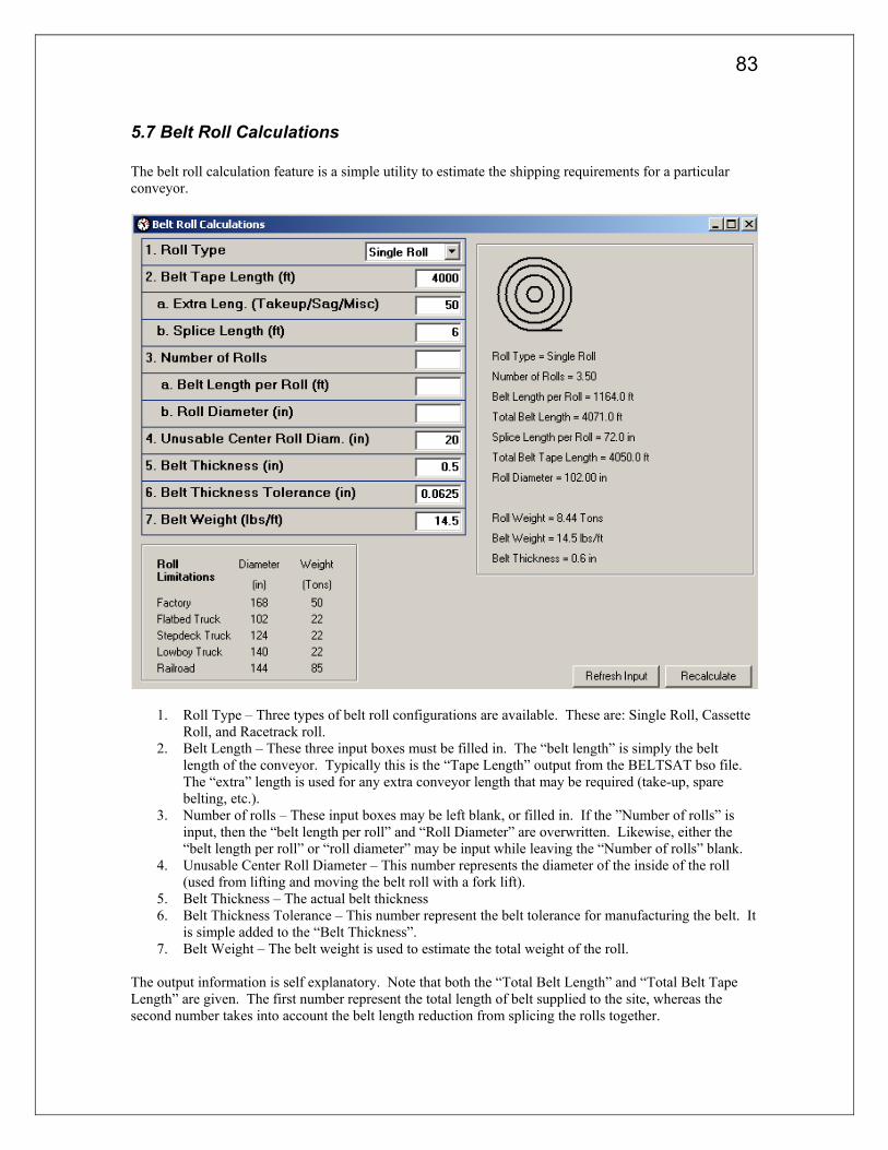
83
5.7 Belt Roll Calculations The belt roll calculation feature is a simple utility to estimate the shipping requirements for a particular conveyor.
1. Roll Type – Three types of belt roll configurations are available. These are: Single Roll, Cassette Roll, and Racetrack roll.
2. Belt Length – These three input boxes must be filled in. The “belt length” is simply the belt length of the conveyor. Typically this is the “Tape Length” output from the BELTSAT bso file. The “extra” length is used for any extra conveyor length that may be required (take-up, spare belting, etc.).
3. Number of rolls – These input boxes may be left blank, or filled in. If the ”Number of rolls” is input, then the “belt length per roll” and “Roll Diameter” are overwritten. Likewise, either the “belt length per roll” or “roll diameter” may be input while leaving the “Number of rolls” blank.
4. Unusable Center Roll Diameter – This number represents the diameter of the inside of the roll (used from lifting and moving the belt roll with a fork lift).
5. Belt Thickness – The actual belt thickness 6. Belt Thickness Tolerance – This number represent the belt tolerance for manufacturing the belt. It
is simple added to the “Belt Thickness”. 7. Belt Weight – The belt weight is used to estimate the total weight of the roll.
The output information is self explanatory. Note that both the “Total Belt Length” and “Total Belt Tape Length” are given. The first number represent the total length of belt supplied to the site, whereas the second number takes into account the belt length reduction from splicing the rolls together.

84
5.8 Material Loading Profile This is another simple feature to help the engineer visualize the conveyor loading.
The standard input variables are self explanatory. The “Banking Angle” is only available for the 3-roll idler set and represent the material profile in a horizontal curve. The “Idelr center length” defaults to “0.37 x belt width” but can also be input. For the 4/5 roll configurations the “Upper Wing Trough Angle” and the “Lower Wing Belt Length: may be entered independently. The output for this features consists of the following:
1. Actual Percent Loading – This is the actual material loading on the belt. 2. Actual Edge Distance – This is the Actual edge distance of the material 3. CEMA Percent Loading – This is the CEMA material loading. This number assume the belt
is fully loaded when the material is at the CEMA “standard edge distance” (0.055 * belt width + 0.9 inches).
4. CEMA Edge Distance – This is the actual edge distance minus the CEMA standard edge distance (0.055 * belt width + 0.9 inches).
5. Material Depth – The depth of the material from the bottom of the belt to the top of the material.
5.9 Belt Feeders
The belt feeder calculations are based off K.S Manjunath and A.W. Roberts papers entitled “Wall Pressure-Feeder Load Interactions in Mass Flow Hopper /Feeder Combinations”, Parts I & II. These two papers can be found in “Bulks Solids Handling” Volume 6, Number 4, August 1986, and in Volume 6, Number 5, October 1986. The design should obtain the above papers as they describe the input variables used in the belt feeder calculations in detail.

85
5.10 Pulley Design The pulley design window allows quick calculations of basic pulley parameters. There are two analysis methods available. The first method is based off of the ANSI/CEMA B105.1-1992 specification for welded steel conveyor pulleys with compression type hubs. All values are directly calculated from this specification. This specification states that it ”SHOULD NOT BE USED WITH STEEL CABLE AND OTHER HIGH MODULUS BELTS”. The second analysis method is the advanced method. This method calculates the shaft bending and torsional stresses based on static force analyses. It will calculate the required shaft diameter, shaft turndown ratios (if applicable), pillow block bearing sizes, and bearing life. A library of standard SKF bearing sizes has been included.
Input Variables

86
Get Input Parameters for This options allow the user to quickly input all required parameters (tensions, wrap angles, belt width, etc.) from a pulley in the current BELTSTAT output file.
Analyses Method
Selects either the ANSI/CEMA B105 specification analysis or the advanced CDI analysis method.
ANSI/CEMA – Calculation base directly from the CEMA/ANSI B105.1 specification for welded steel conveyor pulleys with compression type hubs. Advanced – Calculates pulley diameters, shaft sizes, turndown ratios from static analysis methods. Also select pillow block bearing sizes and properties from the SKF bearing catalog.
Belt Width (required)
Width of the conveyor belt. This input is used to calculate an appropriate pulley face width and determine the PIW of the belt for the input tension values.
Face Width The face width of the pulley.
Pulley Diameter The diameter of the pulley
T1 Tension
The incoming T1 tension of the pulley. Note that CEMA states that running tensions may be used as long as the acceleration tensions do not exceed 150% of the running tensions, BELTSTAT defaults to the “ACCELERATION” belt tensions for a more conservative design.
Belt Direction (checkbox)
If this box is check then the incoming belt tension vector is assumed positive. (see figures on next page)
Entry Angle The angle at which the T1 tension vector enters the pulley. (see figures on next page)
Wrap Angle
The wrap angle of the belt around the pulley. (see figures on next page)
Clockwise (check box) If this box is checked the belt is assumed to wrap in the clockwise direction from the T1 tension vector to the T2 tension vector. If this box is unchecked then a counter-clockwise direction is assumed.
T2 Tension
The belt tension exiting the pulley.

87
Definition of belt directions and wrap angles
Examples of various pulley configurations

88
Pulley Weight The weight of the pulley and shaft assembly.
Shaft Diameter
The diameter of the pulley shaft in 1/16 inch increments. BCMF (Bearing Centers Minus Face)
The total distance between bearings and the pulley face. BCMF = Bearing Centers – Pulley Face Width
Overhung load
An additional weight located some distance outside of the bearings
Overhung Load angle The angle which the overhung load makes with respect to the horizon.
Overhung Load Distance The distance from the bearing to the overhung load
Factor of Safety
The factor of safety of the pulley assembly
Yield Strength The yield strength of the material. Standard values give by the B105.1 specification are: 32,000 psi for C 1018 45,000 psi for C 1045 60,500 psi for C 4110 (annealed)
Actual Shaft Fatigue Limit (Sf*) ½ the value of the ultimate tensile strength of the material. Standard values give by the B105.1 specification are: 29,000 psi for C 108 41,000 psi for C 1045 47,500 psi for C 4110 (annealed)
Correction Factors (K)
Values used to obtain a “corrected” shaft fatigue limit (Sf). Sf = Ka * Kb * Kc * Kd * Ke * Kf * Kg * Sf*
Belt speed Velocity of the belt conveyor. Used to calculated bearing life properties.
Allowable angular deflection The allowed angular deflection at the hub.
Shaft Turndown Ratio
The turndown ratio for the shaft. This has a default value of 0.75 and can not be below 0.5. Turndown Diameter = Shaft Diameter * Turndown Ratio
Turndown Fillet Radius
The fillet radius for the shaft turndown

89
Shell Thickness
The thickness of the pulley shell. This value is only used to calculate the pulley weight. End Disk Thickness
The thickness of the pulley shell. This value is only used to calculate the pulley weight.
5.11 Idler Mass Calculations BELTSTAT v7.0 now inputs both the idler mass and the idler wk^2 factor. Although BELTSTAT has all the standard CEMA idler mass and wk^2 look tables built in, this utility can be used for other non-standard idler sets. If the idler shell thickness is known this table will result in a more accurate estimation of the actual idler mass and inertia.

90
5.12 Loading On/Off The load on/off feature simple run the current conveyor configuration while loading and unloading each flight. Output plots include:
1. Total Power 2. Maximum Belt Tension 3. Minimum Belt Safety Factor 4. Minimum Belt Tensions 5. Maximum Belt Sag.
This x-axis of the output plot is given as function of time. This is allows the designer to better understand how the conveyor is functioning. The “PLUS SIGN” in the plot designates the point at which the conveyor is fully loaded. After this point, the conveyor is unload until it is completely emptied.

91
5.13 Multiple Design Runs This feature allows the user to easily select a range of values for a particular input variable and determine how it effects various output parameters. The “Load On/Off” option loads and unloads each conveyor section and reruns the BELTSTAT calculations for each load case. The user can then plot the conveyor power (or any other output variable) as a function of loading/unloading times. This option is often useful when examining transient conditions.
In the above case the conveyor tonnage was select as the input variable. BELTSTAT ran 10 calculations from 0-100% of the Design Tonnage (0-3000 T/H for this conveyor) The total power was selected as the output variable. Valid Input Variables are: Temperature Tonnage % (as a percentage of the Design Tonnage in the Material Properties window) Belt Width Belt Speed Idler Spacing* Valid Output Variables are: Total Power Maximum Belt Tension Belt Safety Factor *Idler Spacing - Idler spacing allows the user to vary the idler spacing for both the carry and return sides of the conveyor. Furthermore, the user can ONLY vary the Carry (or Return) side idler spacing by inputting the same "Start Value" and "End Value" for the Return (or Carry) side.
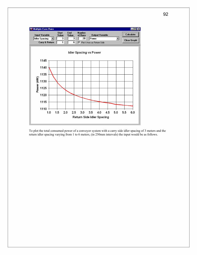
92
To plot the total consumed power of a conveyor system with a carry side idler spacing of 3 meters and the return idler spacing varying from 1 to 6 meters, (in 250mm intervals) the input would be as follows.

93
5.14 Microsoft Work Reports This option allows the designer to generate standard Microsoft Word data files. This feature is very useful since these data files and plots can be E-mailed to non BELTSTAT users (clients, your boss, your best friend, who ever you wish!). The user MUST have Microsoft Word 97 or Word 2000 installed to use this feature. Furthermore, Word macros must be enables to use this feature. To enable Microsoft Word macros open Word and select “Tools / Macros / Security”. Then select either “Medium” or “Low”.
If the “Current Element Table View Window” checkbox is selected then the current element table profile view will also be included in the report. It is often useful to first open the element table, and then “zoom in” on the head or tail section of the conveyor. Once you have the profile window how you want it, select “Create Word Report” from the “Professional” menu and check the “Current Element Table View” checkbox . The figure below shows an example of the head station of a dual drive conveyor with a belt turnover. These figures are very useful when writing conveyor reports or submitting a design to a client.
Example of the head drive station output directly from BELTSTAT

94
Belt tension profile generated by BELTSTAT and exported to Microsoft Word.

95
6.0 EXAMPLES The following five examples will step the user though most of the commonly used features of the BELTSTAT program. A summary of each example is as follows:
#1 – This example will simply introduce the user to the most commonly used features of BELTSTAT. It will explain how to quickly build and analyze a conveyor system. #2 – This example will explain how to input complex conveyor geometry’s in the BELTSTAT program. It will discuss the Element Table in detail and describe each of its input variables. #3 – This example will introduce the user to convex and concave curve analysis. It will describe how generate both types of curves and explain the results of the curve analysis. #4 – This example will introduce the user to many of the professional features found only in the professional version of BELTSTAT. IT will explain how to quickly generate and analyze “worst case” design scenarios. #5 – Example #5 will demonstrate how to used multiple drive and brake configurations with a fixed take-up.
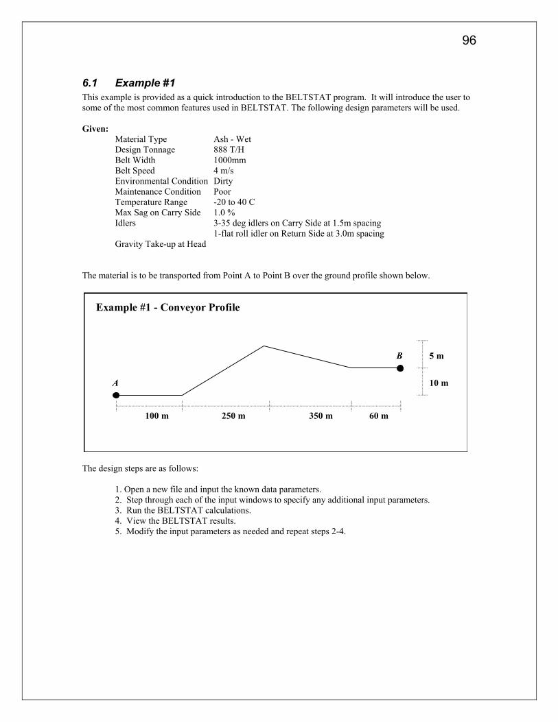
96
6.1 Example #1 This example is provided as a quick introduction to the BELTSTAT program. It will introduce the user to some of the most common features used in BELTSTAT. The following design parameters will be used. Given: Material Type Ash - Wet Design Tonnage 888 T/H Belt Width 1000mm Belt Speed 4 m/s Environmental Condition Dirty Maintenance Condition Poor Temperature Range -20 to 40 C Max Sag on Carry Side 1.0 % Idlers 3-35 deg idlers on Carry Side at 1.5m spacing 1-flat roll idler on Return Side at 3.0m spacing Gravity Take-up at Head The material is to be transported from Point A to Point B over the ground profile shown below.
100 m 250 m 350 m 60 m
10 m
5 m
AA
BB
Example #1 - Conveyor Profile
The design steps are as follows: 1. Open a new file and input the known data parameters. 2. Step through each of the input windows to specify any additional input parameters. 3. Run the BELTSTAT calculations. 4. View the BELTSTAT results. 5. Modify the input parameters as needed and repeat steps 2-4.
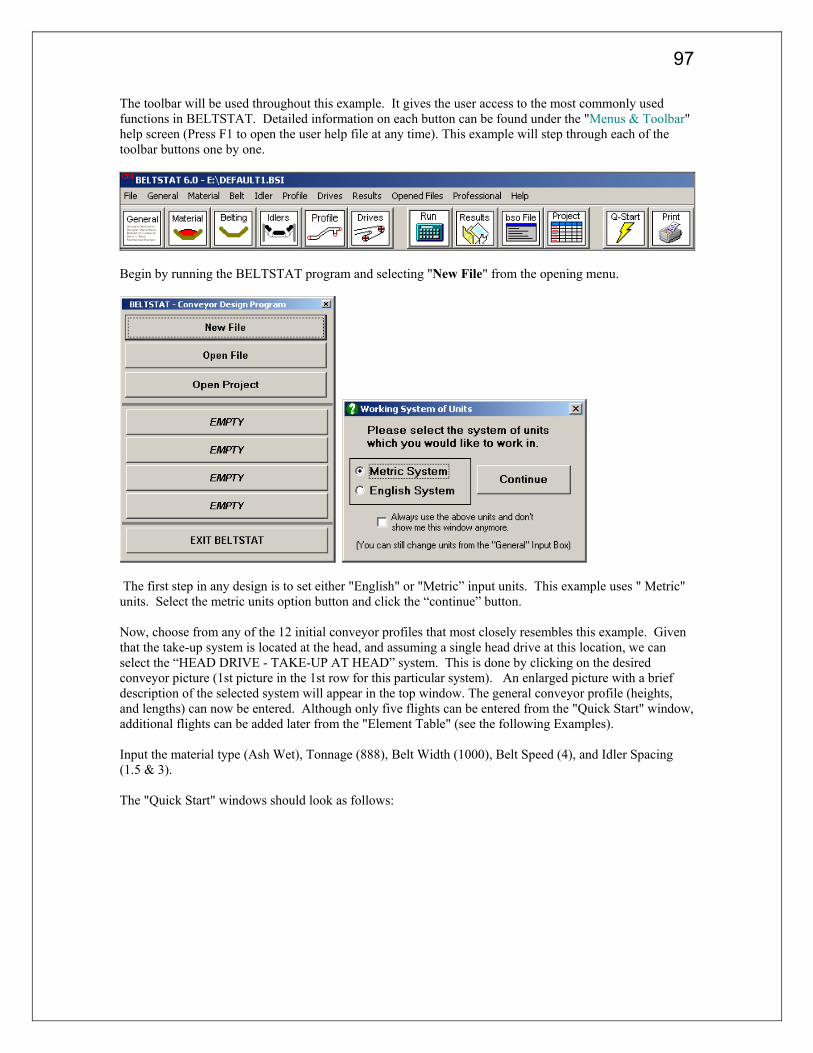
97
The toolbar will be used throughout this example. It gives the user access to the most commonly used functions in BELTSTAT. Detailed information on each button can be found under the "Menus & Toolbar" help screen (Press F1 to open the user help file at any time). This example will step through each of the toolbar buttons one by one.
Begin by running the BELTSTAT program and selecting "New File" from the opening menu.
The first step in any design is to set either "English" or "Metric” input units. This example uses " Metric" units. Select the metric units option button and click the “continue” button. Now, choose from any of the 12 initial conveyor profiles that most closely resembles this example. Given that the take-up system is located at the head, and assuming a single head drive at this location, we can select the “HEAD DRIVE - TAKE-UP AT HEAD” system. This is done by clicking on the desired conveyor picture (1st picture in the 1st row for this particular system). An enlarged picture with a brief description of the selected system will appear in the top window. The general conveyor profile (heights, and lengths) can now be entered. Although only five flights can be entered from the "Quick Start" window, additional flights can be added later from the "Element Table" (see the following Examples). Input the material type (Ash Wet), Tonnage (888), Belt Width (1000), Belt Speed (4), and Idler Spacing (1.5 & 3). The "Quick Start" windows should look as follows:

98

99
At this time the BELTSTAT calculations could be ran by clicking the "RUN" button on the tool bar. However, before running the calculations we will step through each of the input windows one at a time. Click the "General” toolbar button. The general input window will appear. Most of the information in this window is optional, and does not affect the actual BELTSTAT calculations. This information is however very useful for future reference and is found on the BELTSTAT output files and hard copy printouts.
There are a few very import input parameters found in the "General" input window. Both the input and output units are set here. Input and output units can be different. Also note that when switching between "Metric" and "English" input units, the input values themselves do not change. For example, if you started the design in metric units and have a conveyor length of 100m, then switch to English units, the length changes to 100 ft (not 328 ft). Although changing the inputs units is rarely done midway through a design, changing the output units is quite common. For this reason, the user can be working in one system of units and quickly switch the output units to the other system and rerun the BELTSTAT calculations. For example, a designer working in metric units may want to know the belt power in HP, and belt strength in PIW. He/she can simply change the output units, rerun the calculations, and the results will be shown with the new units. Another important input parameter is the Analysis type. CDI has developed, tested, and verified various methods for calculating conveyor tensions and power requirements. These methods are based on the conveyor type (troughed or pipe conveyor) and the rheological rubber properties of the specific belt (Goodyear, Bridgestone, Dunlop, and many other manufactures and rubber compounds). Currently however, CDI only markets two of these analysis methods. The first, "Modified CEMA" is just that, a modified CEMA analysis method. Although it uses many of the standard CEMA conventions and tables, CDI has expanded these tables to include the effects of non standard idler troughing angles, vertical curve pressures, modified the calculations to be used for extended conveyor lengths, as well as many other additional features. The second method calculates the power consumption based on the "Behrens-Schwarz " methodology. For this method the Ky values are calculated according to Ky calculations formulated by Behren’s and Schwartz. On large belts, or belts with large idler spacing (greater than 6.0 feet), this analysis type is suggested regardless of belt construction. Now click on the "Material" toolbox icon. The "General" window will disappear and the "Material" window will appear. A detailed description of each of these input variables is found in the "Material" section of the help file. Remember that at any time you may press the “F1” key for further information on the desired topic.

100
The "Material Type" and "Tonnage" have already entered. From the given data, set the "Environmental Condition" (Dirty), "Maintenance Condition" (Poor), and "Minimum Temperature" (-20 C).
Continuing on through the toolbar icons click the "Belt" Properties. The belt width and speed have already been specified in the "Quick Start" window, therefore no other items need to be changed.
In general, many of the parameters in the "Belt" window can be left blank (In fact they all may be left blank except for the Maximum Sag). Unlike other conveyor design programs, BELTSTAT does not require every input variable to be specified. This shows the power of BELTSTAT over many other conveyor design programs. BELTSTAT has very powerful internal lookup tables and calculation routines to automatically calculate variables that user have not yet specified or are unknown at the current time. BELTSTAT can therefore be used in the early design stages of a conveyor system to determine critical design parameters such as take-up size, belt speeds, belt properties, etc. This is obvious advantage over other design programs that required all data to be known in advance. Notice that #3, the belt type, is left

101
blank. BELTSTAT will choose a nylon, polyester or steel cord belt type based on specific internal calculation routines. Once a design parameter is known however, it should be entered into the program so that BELTSTAT does not calculate some other value for it. For this example, we knew the belt speed and belt width, and therefore specified them. Now select the "Idler" Information window. This is where the number of idlers rolls, and roller angles are specified. The idler type can also be selected. For this example leave the idler type blank and allow BELTSTAT to select an appropriate type. If individual idler properties are known (size, seal frictions, rotating weights, etc.) the user may specify the “Idler Name” as "Other" (or any other name except for the built in types) and enter the appropriate parameters. Additionally, the user can create a custom library of commonly used Idler types by choosing "New Idler" (located in the Idler Name list) and then inputting the name and properties for the particular idler series (see "Idler Inputs").
The next input window is the conveyor "Profile" input window. Two windows appear when the "Profile" button is selected from the toolbar. The first is the “Profile Input Window” commonly referred to as the "Element Table". This input window is where the conveyor geometry, drive and pulley locations, take-up location, vertical curve locations, conveyor loading, and other information related to the overall physical geometry of the system are input. Conveyor flights may be added or subtracted, pulley diameters and wrap angles changed, vertical curves specified, and much more. The conveyors profile always begins with the first element on the carry side of the conveyor. For this particular system BELTSTAT has already added a small transition section (Flight #1) and a skirtboard section (Flight #2). Since we specified the belt width and speed in the "Quick Start", appropriate transition and skirtboard lengths were automatically calculated. We will discuss the "Element Table" in much more detail in the following examples. For now, leave all the input parameters as they are.

102
The second window shows a visual representation of the conveyor system. The user can "zoom" into a specific area of the conveyor system by drawing a box around the area to be magnified. Simply hold down the left mouse button to draw a box around the area which you would like to zoom in on. A holding down the right mouse button will "grab" the conveyor and allow the user to freely move the system around, positioning it in the window as they like (release the right mouse button to drop it). Additionally, and if available, holding down the middle mouse button will allow the user to zoom in and out of the current window by moving the mouse up and down. The command buttons on the left may also be used for these operations.
Select “Drives” from the toolbar to open the final input window. Here information regarding the drives and take-up system is input. Individual parameters can be specified for each drive. See the "Drive Window” help window for more information about the specifics of each input parameter. For now leave the input parameters as they are and allow BELTSTAT to calculate the majority of the parameters.

103
We are now ready to run the BELTSTAT calculations. This is done by either clicking the "RUN" button on the toolbar or by pressing the F4 function key. The "Results" window will automatically appear once the calculations have been completed.
This window shows a quick overview of the current design. More detailed information can be obtained by selecting the “DATA” button in the lower right, and then choosing any of the specific areas of interest (Belt information, Drive information, take-up information, etc.). From the "Results" window we can quickly spot any problem areas in the current design. Variables that are highlighted in red are potential trouble spots. We can immediately identify a problem with the current take-up tension. BELTSTAT has chosen a take-up tension of 14.2 kN. This value was calculated from the Maximum SAG criteria of 1.0%

104
that we specified earlier. Two crucial take-up output parameters are the "Take-up Diff Drv" and "Take-up Diff SAG". These values represent the "extra" take-up tension. This "extra" tension is required since take-up hysteresis is not accounted for in BELTASTAT and should be calculated based on the physical geometry of the take-up system (number of bend pulley, cable diameter, etc). The extra tension also acts as a "Safety Factor" which should be used in any design. A positive number specifies that there is insufficient take-up tension available. In this particular case the "Take-up Diff SAG", which is the take-up differential based on the "Maximum Allowable Belt SAG" is acceptable (3.8 kN of extra take-up tension). The take-up differential based on the drives, however is positive (2.3 kN). The governing case is shown in the next two rows as Drive #1 and takes place during conveyor acceleration. So how can we fix this? First, let’s take a look at the "DATA", "MOTOR" results window shown below.
From line 13 we see that BELTSTAT Selected an acceleration time of about 21.8 seconds. This is based on the default "Starting Torque Limit" (Item #5) that was specified in the "Drive" input window of 135% of the Motor Nameplate. By also checking the drive tension ratios ("DATA", "TR") we see that the tension ratio for the acceleration case has been exceeded. With this information, we have many different options at this point. For example we could change any of the following items: 1. Reduce the motor "starting torque limit" 2. Increase the drives acceleration friction factor 3. Specify a longer acceleration time 4. Increase the take-up tension 5. Change the take-up location 6. Increase the drive wrap angles 7. Add additional drives There are of course other options, but for this simple example, we will set the acceleration time to 40 seconds. To do this click “Drives” on the toolbar to open the “Drive” input window, and enter 40 for an acceleration time in line #9.

105
Rerun the BELTSTAT calculations by click the “RUN” button or by pressing the F4 function key.
Now, going back to the Summary Table ("Main", "Summary") we can see that the take-up system limiting case is the under the steady start running condition. Although the "Take-up Diff Drv" value is now negative (-50 N) there is no "safety factor" in the design. A higher take-up tension should therefore be determined to include hystersis effects and other design factors. For now, lets assume we need an additional 5% belt tension to overcome take-up hysteresis and another 10% for dynamic conditions and other factors. Therefore we have; 14.2 x 1.15 = 16.3 kN of required take-up tension.

106
Setting the take-up tension to 16300 and rerunning the BELTSTAT calculations, we see that the take-up tensions, take-up differentials, and maximum belt SAG are all within acceptable values.
We can plot the belt tensions or by clicking the "Plot" button in the lower right corner of the results windows, and then selecting the "Running", or "Acceleration", plot. A hard copy of any of the output windows can be sent to the printer by simply clicking the “Print” button on the toolbar.

107
We may have left the take-up tension blank and allowed BELTSTAT to continue to calculated new take-up requirements as we modify other design parameters. This however, concludes this example. This is not to say the design is finished, in fact it is far from done! We can still look at many different conveyor aspects such as idler types, idler spacing, different belt speed, and the list goes on. Experiment with this example yourself. Change belt speeds, tonnage, flight lengths, or any of the other input variables until you feel comfortable working with each of the input windows. Also, for this system we have only calculated the tensions for the "Fully Loaded" conveyor system. Other loading patterns, such as only loading the inclined portions of the belt, should also be analyzed (see Example #3). You may also want to save your work at this point. Select “File”, “Save File As” and enter a directory and filename to save the current input file. It is VERY important to remember that BELTSTAT is a STATIC analysis program. It will calculate acceleration times, brake torque requirements and braking times, but these calculations are based on static calculations. For many conveyor systems a "DYNAMIC ANALYSIS" is required. In a dynamic analysis the dynamic equations of motion are calculated in a forward time stepping procedure. Unlike the steady state analysis, belt tension can and will vary at each flight along the conveyor as the system is started and stopped. This is especially true of long overland systems where strong dynamic tension waves can be present. Conveyor Dynamics, Inc. has developed a dynamics analysis program with the tradename BELTFLEX. This program has been extensive tested and verified by field measurements on conveyor systems around the world. If you feel your conveyor system may require a "Dynamic Analysis" please contact CDI.

108
6.2 Example #2 This example will demonstrate how to input a conveyor’s geometry into the BELTSTAT program. It will focus on the “Element Table” and its input variables. The conveyor geometry will first be created using the “Conveyor Quick Start” window. Then a new “blank” file will be created and the entire conveyor profile will be created manually. The following design parameters will be used for this example. Given: Material Conveyed Wet Ash Design Tonnage 1888 T/H Bulk Density 720 kg/m^3 Surcharge Angle 25 Deg Environmental Condition Dirty Maintenance Condition Poor Temperature Range 0 to 40 C Belt Width 1000 mm
Max SAG on Carry Side 1.0% Gravity take-up & drive system at the head
Conveyor Profile: STATION ELEVATION LENGTH HEIGHT 0 0
50 0 50 0 140 10 90 10 210 5 70 -5 250 5 60 0 340 15 70 10 420 5 80 -10 490 5 70 0
Example #2 - Conveyor Profile
0
5
10
15
20
0 50 100 150 200 250 300 350 400 450 500
Station (m)
Elev
atio
n (m
)

109
To begin, open BELTSTAT and click the “New File” button. Select metric units and click “continue”. As in Example #1 select the “HEAD DRIVE - GRAVITY TAKE-UP AT HEAD” system (1st picture in the 1st row). Enter the lengths and heights of the first four elements. Also enter the material type, belt width, and design tonnage. The “Quick Start” window should look like the following.
Click the “Profile” button to bring up the “element table and profile window. They will appear as follows.

110
The initial 50m conveyor flight has automatically been cut up into three separate flights. The first flight is the transition flight. It represents the length of belt from the tail pulley to the skirtboard. The next flight is the skirtboard. This flight is designated by an “S” for “skirtboard” in the Flight ID column of the element table. The “Conveyor Loading” column also contains the design tonnage of 1888 T/H. The skirtboard and conveyor loading are required to account for the acceleration of the material as it is loaded on the conveyor system. Although we were only able to input the first five flights in the “Quick Start” window, we can now add as many additional ones as we desire. Select flight #7 and click the “Insert below” button on the right side of the element table (or press F6). Insert two additional flights. The element table and conveyor profile should like as follows.
Now from the initial conveyor profile information, enter the correct flight lengths and heights for flights 8 and 9.
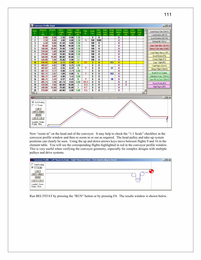
111
Now “zoom in” on the head end of the conveyor. It may help to check the “1-1 Scale” checkbox in the conveyor profile window and then re-zoom in or out as required. The head pulley and take-up system positions can clearly be seen. Using the up and down arrows keys move between flights 9 and 16 in the element table. You will see the corresponding flights highlighted in red in the conveyor profile window. This is very useful when verifying the conveyor geometry, especially for complex designs with multiple pulleys and drive systems.
Run BELTSTAT by pressing the “RUN” button or by pressing F4. The results window is shown below.

112
The next part of this example is a bit more advanced. It will step through the method required to create the above conveyor profile from scratch. For most conveyors, one of the “Quick Start” conveyors systems can be used as a starting point, and then simply modified to meet the required profile. However, it is important for the user to fully understand how the element table functions, and how to build a system from scratch. We will begin by closing the current file and opening a new one. Again select “Metric” units and from the “Quick Start” window select the “No flights” conveyor profile (last button in the last row). Enter the Material Tonnage of 1888 and “Ash Wet” for the material type.
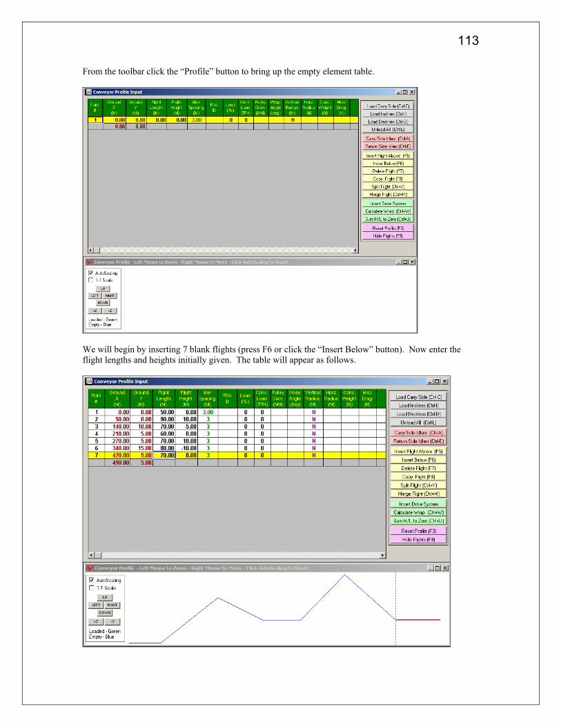
113
From the toolbar click the “Profile” button to bring up the empty element table.
We will begin by inserting 7 blank flights (press F6 or click the “Insert Below” button). Now enter the flight lengths and heights initially given. The table will appear as follows.

114
Now we need to create the take-up system. This could be done by clicking the “Insert Drive System” button found in the lower right side of the element table, and then selecting the gravity take-up system (1st column 3rd row). For this example however, we will enter each flight manually.
Click the “Cancel” button to close this window. To create the take-up system manually we must first insert 5 to 10 blank flights at the end of the profile. Now insert the head drive by entering a “D” in the flight ID of element #8. Note that the “D” will automatically change to “D1” after you press the enter key. This is simply for convenience and indicates that it is the 1st drive of the conveyor system.
You may want to “zoom” in on the head drive at this time so you can watch the take-up system being built as you enter each flight. Also, turn on “1-1 Scaling” to make the scale XY scale 1 to 1. Remember that you can zoom into a specific area by holding down the left mouse button and drawing a box around the area you want to zoom in on. Furthermore, holding down the right mouse button will “grab” the conveyor so you can freely move it around. This takes a little practice, but once you get the hang of it, it’s very easy

115
to quickly zoom in on an any area of the profile. Checking the “AutoScaling” button reset the conveyor profile to its original position.
You should also enter the wrap angle for the drive pulley. Enter 180 in the “Wrap Angle” column of flight 8. Next, enter a short –3.0 meter section of belt to reach from the head pulley to the 1st bend pulley (flight #9). Now enter the bend pulley in flight #10 by putting a “P” in the flight ID. Initially you will notice that BELTSTAT inserts 180 for a wrap angle. All pulley wrap angles must be input into BELTSTAT since the program does not have any basis as to how they should be calculated. BELTSTAT always assume that a positive wrap angle indicated that the belt is warped “CLOCKWISE” around the pulley. For this pulley change the current wrap angle from +180 to –90 degrees.
Now add flights for the rest of the take-up system using appropriate wrap angles and flight lengths. Use a flight height of +/- 10.0 meters for the take-up travel length and insert a “T” for the “take-up” pulley. The element table should appear as follows.

116
Now we are ready to generate the return side of the conveyor. There are only TWO flights used to create the return side. The first is an “R#” or mapped return flight. This flight will simply mirror, or map, a flight on the carry side of the conveyor. For example, a “R5” will map carry flight #5. This command can be used in-groups to map a set of flights as well. For example “R 7 1” will generate and map carry flights #7, #6, #5, #4, #3, #2, and #1. The other unique return flight is the “RS#” flight. This flight may seem odd at first but is VERY time saving! Its purpose is to map a flight from the current position to the beginning of a specified flight. For example “RS7” will generate a flight from the current location (the bend pulley after the take-up) to the beginning of flight #7. This way the user doesn’t have to manually calculate the required flight length. Furthermore, if the take-up lengths are changed (say flight #9), the RS will automatically resize itself. Now the return strand can now be created. First insert a few blank flights (F6). Now enter “RS7” for the flight ID of element 15. After pressing return you will be asked to enter the vertical distance between the carry and return sides of the conveyor. Simply click “ok” to use the default value of 1000mm.

117
In flight #16 enter “R 6 1” to generate flights from flight #6 back to flight #1. Six new return flights have been created. Finally, add a tail pulley in flight #22 and delete any blank or empty flights you may have left. Now any changes you make to the carry side flights will automatically update the return elements.

118
In the first part of this example the 50m flight was cut up into 3 sections (a transition section, a skirtboard section, and the remain length). This can be accomplished by selecting flight #1 and clicking the yellow “Split Flight (Ctrl+Y)” button. Enter “2.5” to create a transition flight and click “ok”. Now create the “Skirtboard” flight by selecting flight #2 and again clicking the yellow “Split Flight” button. Enter 8 for an 8.0 meter long skirtboard section. We also need to tell BELTSTAT that flight #2 is a skirtboard, and that material is being loaded at that location. To do so enter “S” (for skirtboard) in the “Flight ID” column of flight #2. The element table should now look like the following:
The “Load %” column and “Conv Load (TPH)” column will automatically be updated. The “Loading %” column represents the percentage of the conveyor load on the flight. For example if you specify the material tonnage to be 2000 TPH (in the Material input window) and enter 50 in the "Loading %” column, that flight would then be loaded at 1000 TPH (2000 * 0.5). The “Conv Load (TPH)” column is used to specify that material is being LOADED onto the conveyor at flight #2. In this cases the “Conv Load” is 1888 TPH. However if we had two loading points we could load one flight at 1000 TPH and the other at 888 TPH (a total of 1888 TPH). The load percentage would then be 55.5 percent (1000/1888) for all flights between the first and second loading points and 100 percent after the second loading point. Now we need to load material on the Carry side of the conveyor. Click the “Load Carry Side” button on the right hand side of the element table. Notice that flight #1 is not loaded (0 in the “Loading %” column) since it is before the skirtboard. Next change the carry and return idler spacing. This is done by clicking the red “Carry Side Idlers” and “Return Side Idlers” buttons. Use a carry side idler spacing of 1.5 meters and a return side idler spacing of 3.0 meters. Also change the idler spacing of flight #1 and #2 to 0.5 meters by simply clicking on the “idler Spacing” column of flights 1 and 2. These flights were not changed when the “Carry Side Idlers” button was used since the transition and skirtboard flights will typically have a different idler spacing than the rest of the conveyor. The final element table is shown below.

119
That’s it! A bit more work than by using the conveyor “Quick Start” option, but now you have the general idea of how it’s done. Remember you can always press F1 at any time to get even more information on the element table. Once you understand the fundamentals of the element table, almost any conveyor geometry can be built. Multiple drives, booster drive systems, complex pulley geometry’s, you name it! You can now “RUN” the conveyor calculations and change any of the input variables you like. This however, completes example #2. More information on the use of the element table and how to create and modify vertical curves is given in the next example. The reader is encouraged to work with this conveyor to determine an optimum design. Start by changing acceleration times and the take-up tension.
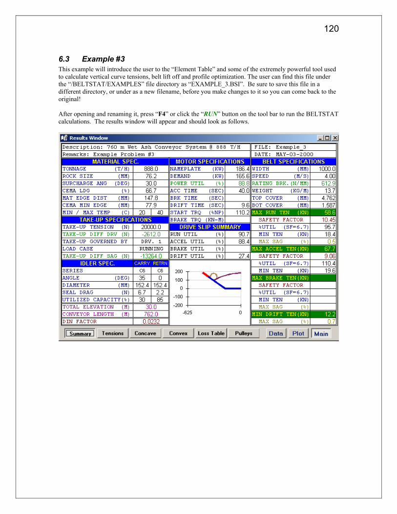
120
6.3 Example #3 This example will introduce the user to the “Element Table” and some of the extremely powerful tool used to calculate vertical curve tensions, belt lift off and profile optimization. The user can find this file under the “/BELTSTAT/EXAMPLES” file directory as “EXAMPLE_3.BSI”. Be sure to save this file in a different directory, or under as a new filename, before you make changes to it so you can come back to the original! After opening and renaming it, press “F4” or click the “RUN” button on the tool bar to run the BELTSTAT calculations. The results window will appear and should look as follows.

121
Lets assume we want to add a convex curve with a 500m radius at the beginning of flight #5. BELTSTAT uses individual discrete elements or “Flights” to mathematically represent a conveyor system. The more accurately the flights lengths and heights reflect the actual conveyor system the more accurate the calculated results. Currently there are only two flights (#4 & #5) that represent the convex segments of the conveyor profile.

122
The tension at the beginning, of each of the flights can be found under the “Results” windows under “Main” “Tensions” and are as is as follows. Beginning of Flight #4 – 23180 Beginning of Flight #5 – 57795 Beginning of Flight #6 – 57403 (same as the tension at the end of flight #5)
As a first approximation to the convex curve we can simply enter a 500m radius at the desired flight location. Select “Profile” from the toolbar (if the profile window is not already opened) and enter 500 in the vertical radius column of flight #5. This tells BELTSTAT that there is to be a 500m radius over the entire length of flight #5. Also notice that BELTSTAT places a 500 M radius at the same location on the return strand (Flight #16). Notice that although this is on flight 4 (vs. Flight 5 on the carry) the point where the calculations are preformed is the same. BELTSTAT will use this radius to calculate an increased pressure on the idler rolls (due to the convex curve) and therefore a slightly higher Ky value for the entire flight.
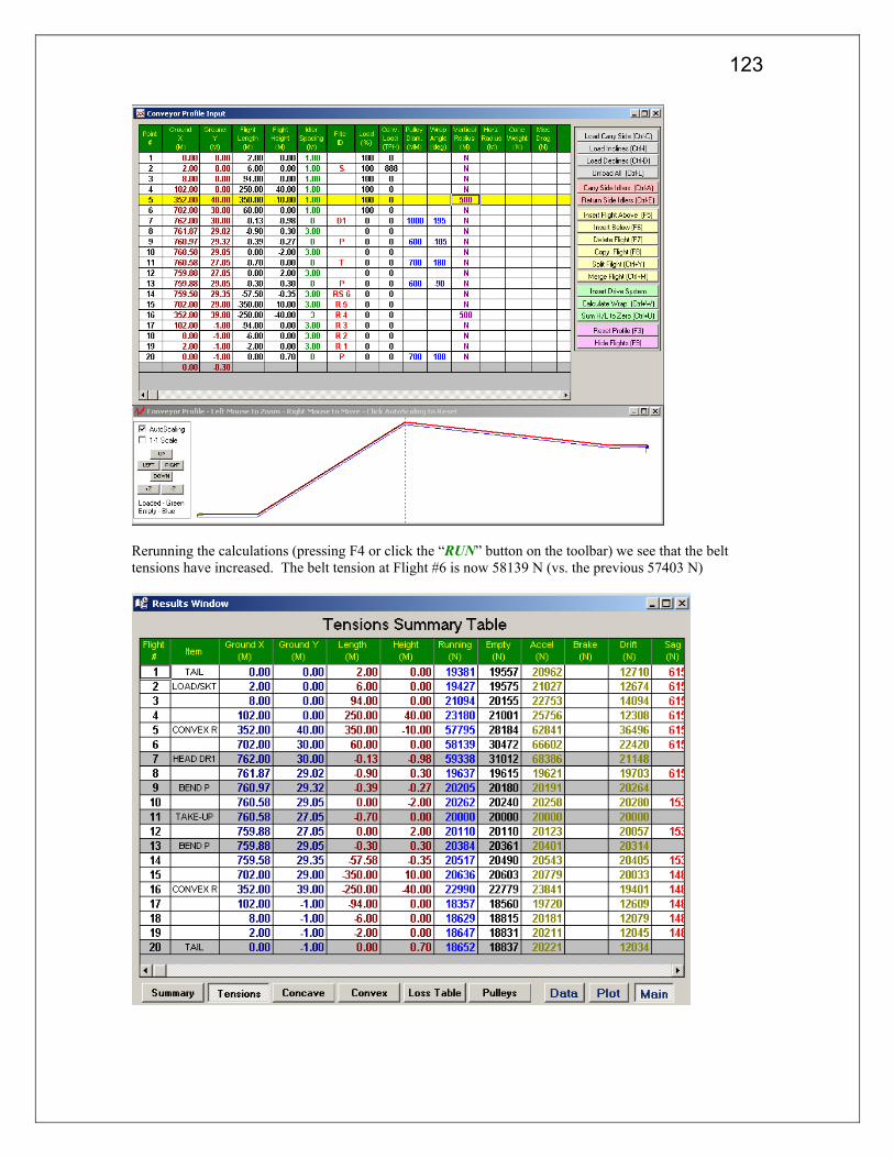
123
Rerunning the calculations (pressing F4 or click the “RUN” button on the toolbar) we see that the belt tensions have increased. The belt tension at Flight #6 is now 58139 N (vs. the previous 57403 N)

124
By including this radius we have also slightly increased the conveyors power. However, this configuration is still not ideal. Although we have specified a radius at flight #5 we have not said anything about flight #4 which would also be part of the 500m radius. We are also assuming that the 500m radius exists over the entire conveyor length, which is incorrect. Furthermore, in real life, the 500m radius will “cut off” the abrupt peak at flight #5 and therefore lower the actual height which the material must be lifted (this can be substantial for many conveyor systems). So what can we do? Here in lies the power of the new BELTSTAT user interface. As we mentioned earlier, the more accurately the conveyor reflect the real profile the more accurate the final results. By “cutting up” the current two flights (#4 & #5) into subflights we can more accurately define the conveyor profile. We do this by simply entering “”V#” into the Flight ID column at the flight we want the profile refined. The “V” tells the program to cut the conveyor into vertical flights. The “#” tell the program how many flights to cut the section into. For example, enter “V6” into the ID column of Flight #5.
This automatically cuts the current two flights up into six new flights as shown on the next page.
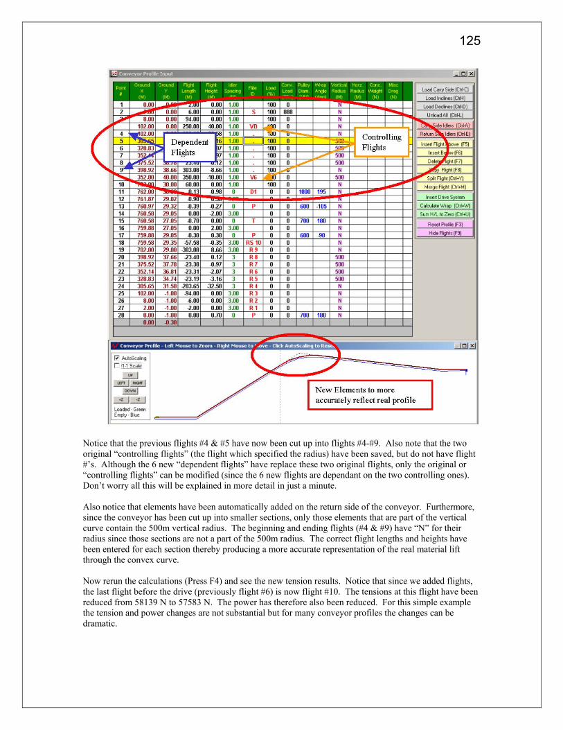
125
Notice that the previous flights #4 & #5 have now been cut up into flights #4-#9. Also note that the two original “controlling flights” (the flight which specified the radius) have been saved, but do not have flight #’s. Although the 6 new “dependent flights” have replace these two original flights, only the original or “controlling flights” can be modified (since the 6 new flights are dependant on the two controlling ones). Don’t worry all this will be explained in more detail in just a minute. Also notice that elements have been automatically added on the return side of the conveyor. Furthermore, since the conveyor has been cut up into smaller sections, only those elements that are part of the vertical curve contain the 500m vertical radius. The beginning and ending flights (#4 & #9) have “N” for their radius since those sections are not a part of the 500m radius. The correct flight lengths and heights have been entered for each section thereby producing a more accurate representation of the real material lift through the convex curve. Now rerun the calculations (Press F4) and see the new tension results. Notice that since we added flights, the last flight before the drive (previously flight #6) is now flight #10. The tensions at this flight have been reduced from 58139 N to 57583 N. The power has therefore also been reduced. For this simple example the tension and power changes are not substantial but for many conveyor profiles the changes can be dramatic.

126
To further demonstrate the flexibility of BELTSTAT lets assume that the elevation of the vertical radius has changed from 40m to 20m, and that the radius has been changed to 1000m. To do this, simply change the first “controlling flight” elevation from 40m to 20m.
Notice that when you change the flight lengths or heights of either of the “controlling flights” all the dependant elements are automatically recalculated to reflect to changes. Furthermore, the return strand is also automatically changed. Now change the vertical radius from 500m to 1000m. Again, all elements on the carry and return sides are automatically refreshed. Before rerunning the calculations lets tell BELTSTAT to output a detailed description of the vertical curve tensions. Under the “General” input window check the box labeled “Curve Report”.

127
Now rerun the calculations (Press F4) and observe the results. Select “Main” & “Convex” to show the convex curve tension results. Both edge, and center belt tensions are shown for the running, empty, accelerating, and drift conditions. Also given are the recommend idler spacing and the individual idler loads. In many cases the idler spacing will need to be increased in areas of small convex curves.

128
Now lets add a concave curve at the beginning of the inclined section of the conveyor. First enter a radius of –400m. The negative sign indicates that the curve will be a concave radius as opposed to a positive radius indicating a convex curve (although BELTSTAT will automatically correct you if you enter the wrong sign). Next replace the “VB” in the element table with a “V4” (“VB” represent the beginning of the vertical curve which already exists). A curve can be cut up into as many flights as desired. Again the more elements the higher the accuracy, however six flights is usually sufficient for most radii. Only four sections are used here to demonstrate the point and since the DEMO version is limited to a total of 35 total flights.

129
We will now have 32 flights and the profile should look like the figure below.
Notice that flight #6 appears both above and below the controlling flight. This is because it is part of both the first and second curves, and is only there for the users convenience. It is the same flight and is only included in the calculations once (press F9 to hide and unhide the controlling and symmetric flights). Also note that if you change the height or length of the “V4” controlling flight, BOTH curves automatically reflect the changes. For example, replace the 20m flight height (highlighted flight below) back to the original 40m, and notice all elements are updated automatically. Your profile should now look like the following.

130
Now rerun the calculations and view the “Main”, “Concave” results window. We can see that for flight #5 the minimum allowable radius (based on belt lift off) is 189 m. Since we have specified a 400m radius belt lift off will not be a problem in this area.
This concludes this example but the user should continue to experiment with this convey system. Try changing the radii and flight or heights lengths. Also remember that different load cases will have different tension values. Rerun the calculations with n the inclined and declined flights loaded (Click the “Load Inclines” button on the element table). To remove a vertical curve simply enter a “Space” in the ID column of the “controlling flight (blank out or delete the “V6” or “V4”). The curve and dependent flight will automatically be deleted.

131
6.4 Example #4 This example is provided to show the user how to use the “Multiple Runs” and “Projects” options of BELTSTAT. Begin by opening “EXAMPLE_4.BSI” from the “*/BELTSTAT/EXAMPLES” directory. Now save the file (“File”, “Save File As”) under a new name such as “EX4-NOR.BSI”, for Example #4, normal conditions. This way the original file can always be referred back to. For this example, assume that the user has designed the above system under “normal” or “expected” fully loaded operational conditions. He/she would like to quickly determine how the system behaves under a variety of other conditions. The designer may ask the following questions: 1. What is the maximum power consumption under any circumstance? 2. How might the conveyor behave under “cold weather” conditions vs. “normal” operating conditions? 3. Could the conveyor ever become regenerative? 4. What is the power consumption and the belt safety factor for various belt speeds or load conditions? In previous versions of BELTSTAT and in other conveyor design programs each of these cases would need to be studied independently. For example, the 1st question of the maximum required power, is a very fundamental, yet complex design parameter. As stated above, the assumption is made that the current design parameters are the “Normal” or “Expected” design parameters. For example, the idler seal frictions and belt weights may have been given by the manufactures. The conveyor is uniformly loaded over is entire length at the design tonnage. But what if the actual belt weight is slightly more (110%) than the manufacture specified? Or, how much is the seal friction of the idlers increased under cold weather conditions? How would that increase affect the power consumption? What is the conveyor loading is not uniform? Using the following assumptions, let’s try to determine the maximum conveyor power. 1. The maximum power occurs when only the inclined sections of the conveyor are loaded 2. The actual belt weight is 5% higher than the manufacture had specified 3. The minimum temperature is –20 C and the idler seal friction increased by 25% at these temperatures. 4. The loading operator overloads the belt by 10%.

132
The first step is to save the file under a new name (“File”, “Save File As”). Call it “EX4-MAX.BSI” for Example #4, maximum power. Click on the “Profile” toolbar button and select the “Load Inclines” button to load the inclined sections of the conveyor. An input box will appear asking for the slope of the inclines to load. A typical value of –0.015 is usually used. A negative number is used since a flat or slightly declined section of belt may still increase the power requirements (is not regenerative). Also stated in the above assumptions was that the conveyor will be loaded at 110%. Therefore the Conv. Load (THP) for flight #2 needs to be changed from 888 to 977. NOTE: THE DEMO VERSION OF BELTSTAT ONLY ALLOWS TONNAGE’S OF 0, 888, and 1888 T/H AND THEREFORE THE TONNAGE MUST REMAIN AT 888 T/H. This number is used to include the materials acceleration effects when transferring from the chute system onto the conveyor belt. It does NOT represent the actual load on the conveyor belt (see “Conveyor Profile” in the online help file). The conveyors actual loading is found under the “Material” input window and will be change later.

133
Now go to the “Belt” input window, and increase the belt weight from 20 kg/m to 21 kg/m (5%).
Next, set the minimum temperature to –20 degrees Celsius in the “Material” input window. From here the design tonnage can also increase by 10%. The design tonnage should be changed from 888 T/H to 888*1.1=977 T/H. NOTE: THE DEMO VERSION OF BELTSTAT ONLY ALLOWS TONNAGE’S OF 0, 888, and 1888 T/H AND THEREFORE THE TONNAGE MUST REMAIN AT 888 T/H.
In the “Idler” window the idler friction can be increased by 25%. The carry side seal friction should be set to 6.7*1.25=8.4 N, and the return side seal friction set to 2.2*1.25=2.8 N. Note that had a “standard” idler been used the seal drag and other variables are fixed internally by BELTSTAT. For this case we selected “OTHER” for the idler type and input the appropriate properties directly.

134
Now rerun the BELTSTAT calculations (by pressing F4), and take a look at the summary table. The new power consumption has increased from the previous 262 kW to 388 kW. The 350 kW motor previous specified is no longer sufficient. Are the above assumptions realistic? That all depends. For many conveyors the above conditions may be even worse, whereas for other systems they may be too stringent. The designer may wish to leave all parameter as they are and only load the inclined conveyor sections to see the power consumption change with out the temperature, seal drag, and increased belt weight effects. Would the single 350 kW motor still be sufficient? Let’s assume the above conditions represent the worst case and move on to the next question. Could the system ever become regenerative? We could follow the same process as before only with the following assumptions:
1. Open the “normal conditions” file, and save it as “EX4-LOW.BSI” for low friction, or low power consumption.
2. Reduce the belt weight (remember, belts covers can wear down significantly and belt weight after 5 or 10 years of operation may be much less than it was originally).
3. Only load the declined sections of the conveyor profile. 4. Increase the temperature to the maximum expected value. 5. Decrease the idler seal friction.
There are of course many other factors that may also come into play for a specific conveyor system, but these are some of the most basic. This may seem very tedious especially when design optimizations, alternate profiles, cost analysis, and other factors come into play. For this reason BELTSTAT has created a “Project” option to quickly create, calculated, and summarize these scenarios and many more. BELTSTAT has the capability to quickly and routinely analyze many of the most common design scenarios.

135
To uses the “Project” feature we must first “CLOSE” any files that are currently open. Now re-open the original “Example 4.bsi “ file and save it as “EX4-MAS.BSI”. Next Select “PROJECT” from the toolbar. The following window will appear.
This window was developed to quickly aid the designer in finding the worst case information on the desired conveyor system. Each of the six input columns represents a specific scenario or case of interest. They are as follows: RUN 1- Normal Operational Case (i.e. no parameters are changed). RUN 2- Fully Loaded Hi Friction - increased idler friction, increased belt weight. RUN 3 – Fully Loaded Low Friction - decrease friction, decreased belt weight. RUN 4 – Extra – a “user” specified case which maybe important for the specific conveyor design. RUN 5 – Empty Belt - normal operational conditions. RUN 6 – Maximum Power – inclines loaded, increased belt weight, increased seal friction. RUN 7 – Maximum Drift / Reintegration – declined loaded, low friction, low belt weight. Each of these cases can be freely modified to meet a specific design specification and then stored for future reference. CDI has included some typical design values for these specific cases, but those values may easily vary from one conveyor design to the next. Take a minute to become familiar with this input window and think about the input values that you would use for your conveyor design projects. Now lets uses this table to quickly recalculate to maximum power we examined earlier. Modify the column for RUN 6, the maximum power case. Simply enter the new design tonnage, minimum temperature, belt weight multiplier, and the seal friction multiplier. Note that some variables have a multiplication sign (*) after them and some have a (+) sign. This indicates whether the input value should

136
be multiplied by, or added to the current input value. For example, in this case the belt weight was given (perhaps by the manufacture). It was then assumed that the actual belt could weigh as much as 5% more than this value. Thus a multiplication factor of 1.05 is entered. In other case the belt weight may not be know and left blank. In this case BELTSTAT would calculated a belt weight based on the belt type and the top and bottom cover thickness. The uses may have specified the top and bottom cover thickness and had BELTSTAT calculate an appropriate belt weight. In this case, to calculate the maximum belt weight, the users could add a specified amount (say 1mm) and have BELTSTAT recalculate a new weight based on that value. For the worn belt case the designer may have assumed that 3mm of wear had occurred on the belt cover and entered –3 for a top cover thickness.
The values for the other RUN cases could also be modified at this time, but for now we are only concerned with the maximum power cases. Once you have entered the information into the table click the “Create Project Files” button. By pressing this button you are telling BELTSTAT to create six new input files, all based on the original “EX4-MAS.BSI” file. Each file will be created, and modified by the parameter in the above input table. Once the files have been created, two new command buttons will appear. The first is labeled “Update Files”. When this button is press the current files are updated to match the input table. Then next button is labeled “Run Project Files” and does just that. It reruns all 7 files (the initial file and the six new files) and then displays a summary table of the results for each file. Click the “Run Project Files” button now.

137
This window shows a summary of all seven cases and is extremely useful when analyzing complex conveyor designs. Notice that the power consumption of 388 kW matches the previous calculations. Click the “Print” toolbar button to print out a hardcopy of the results.

138
So what about the regenerative case? Let’s go back to the input table. Click the “Input” button again, and enter the following information in the column labeled RUN 7.
1. As before, assume 110% material loading and enter 977 as a design tonnage. 2. Set the maximum and minimum temperatures to 40 C. 3. Assume that the belt covers have worn down and the belt weight is therefore reduce to 80% of
it original weight. 4. The idlers seal friction is reduced by 25%. 5. Use the standard CEMA Ky reduction factor of 0.67.
Now click the “Update Files” button to update the files so they reflect these changes. Then click the “Run Project Files” to rerun the BELTSTAT calculations. Notice that the power for RUN 7 is now –19 kW, and therefore the system could go into regeneration! However, the purpose of this example is not to dwell on the specifics of this particular design, but to emphasize the importance and learn how to quickly check any design for possible problem areas, or loading case you may have otherwise missed.

139
If you want to go back and look at a specific case in more detail simply select it from the “Open Files” main menu. All seven cases are listed and can easily be toggled between by holding down the “SHIFT” key and pressing one of the “Function keys”.
It may seem cumbersome to have so many files for one conveyor design, and therefore have incorporated a “Project” option into BELTSTAT. The entire project including the “Normal” case, the six standard cases, and the case input table used to create the standard cases, can be save in one location by simple selecting “Save Project” from the “File” menu.
Project file can be opened by click “Open Project” button from the opening BELTSTAT window.

140
This almost concludes this example, but before leaving let’s take a look at the final question proposes at the beginning of this example. 5. What is the power consumption and belt safety factors for various belt speeds or load conditions? The answer to this question lies in the “Multi Run” window. Click the “Mult Runs” button on the toolbar. For the “Input variable” select “Belt Speed”. To analyze belt speeds from 2.0 to 5.0 m/s enter 2, and 5 in the starting and ending value boxes. Now click the “Calculate” button. BELTSTAT will run 10 times and display the results for each run. You can change the “Output Variable” to show minimum belt safety factors, maximum belt tension, and other relevant parameters. You can also select other input variables, such as the idler spacing, to quickly optimized specific design parameters.
Although this concludes this example, continue experimenting with but the “Multiple Case” table and the “Multiple Runs”. Also remember that the online help file can be accessed at any time by press the F1 function key.

141
6.5 Example #5 – Fixed Take-up This example will illustrate a conveyor with a fixed take-up, dual head drive, and a tail brake. The conveyor profile has both an incline and decline section. The following design parameters will be used for this example. Given:
Material Conveyed Copper ore Design Tonnage 2000 T/H Bulk Density 1600 kg/m3 Surcharge Angle 25 Deg Maximum lump size 200 mm Environmental Condition Dirty Maintenance Condition Poor Temperature Range 0 to 40 C Max SAG on Carry Side 1.0% Idler spacing (carry x return) 1.5 x 3 m Idler type on carry CEMA C6, 35º trough Idler type on return CEMA C6, 10º trough Take-up & drive system at the head Take-up type fixed Tail brake Constant torque Required stopping time 20 seconds
Conveyor Profile:
STATION ELEVATION LENGTH HEIGHT 0 0 250 -40
250 -40 250 0 500 -40 750 60 1250 20
Example 5 - Conveyor Profile
-50-40-30-20-10
0102030
0 200 400 600 800 1000 1200 1400
Station (m)
500 m Radii
Procedure: 1. Go to Quick Start and select the profile in row 1 column 2 (dual head drive, take-up at head). 2. Input all given information in Quick Start. 3. Close the quick start window and save the file as “exp5.bsi”.

142
4. Go to “Profile” and insert a “D” in Flight ID at line 16 to insert the tail brake. 5. Insert 500 meter concave curves. (See picture below)
a. Insert a 500 meter radius in lines 4 and 5 in the Vertical Radius column. b. Insert a V4 in line 4 in the Flight ID column. c. Insert a V4 in line 7 in the Flight ID column.

143
6. Go to “Drives”, and set Drive 1 and 2 at head to be motors drives, and Drive 3 will be the brake.
d. set power ratio to 1:1:0 (tail pulley does not have a motor) e. set synchronous to 1500:1500:0 (brake synchronous speed = 0) f. set starting torque to 135:135:0 (brake starting torque = 0) g. set motor efficiencies to 95:95:100 (brake efficiency = 100) h. set brake torque ratio to 0:0:1 (drive pulleys at head do not have brakes)
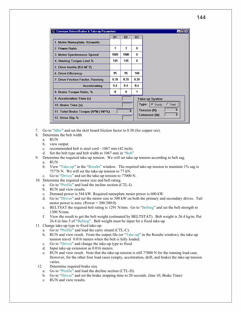
144
7. Go to “Idler” and set the skirt board friction factor to 0.30 (for copper ore). 8. Determine the belt width
a. RUN b. view output c. recommended belt is steel cord - 1067 mm (42 inch). d. Set the belt type and belt width to 1067 mm in “Belt”
9. Determine the required take-up tension. We will set take-up tension according to belt sag. a. RUN b. View “Take-up” in the “Results” window. The required take-up tension to maintain 1% sag is
75776 N. We will set the take-up tension to 77 kN. c. Go to “Drives” and set the take-up tension to 77000 N.
10. Determine the required motor size and belt rating. a. Go to “Profile” and load the incline section (CTL-I). b. RUN and view results. c. Demand power is 544 kW. Required nameplate motor power is 600 kW. d. Go to “Drives” and set the motor size to 300 kW on both the primary and secondary drives. Tail
motor power is zero. (Power = 300:300:0) e. BELTSAT the required belt rating is 1291 N/mm. Go to “Belting” and set the belt strength to
1300 N/mm f. View the result to get the belt weight (estimated by BELTSTAT). Belt weight is 26.4 kg/m. Put
26.4 in line 5 of “Belting”. Belt weight must be input for a fixed take-up. 11. Change take-up type to fixed take-up.
a. Go to “Profile” and load the carry strand (CTL-C). b. RUN and view result. From the output file (or “Take-up” in the Results window), the take-up
tension travel 0.016 meters when the belt is fully loaded. c. Go to “Drives” and change the take-up type to fixed d. Input take-up extension as 0.016 meters. e. RUN and view result. Note that the take-up tension is still 77000 N for the running load case.
However, for the other four load cases (empty, acceleration, drift, and brake) the take-up tension varies.
12. Determine required brake size a. Go to “Profile” and load the decline section (CTL-D). b. Go to “Drives” and set the brake stopping time to 20 seconds. (line 10, Brake Time) c. RUN and view results.

145
d. Required brake torque is 21117 N-m. e. Go to “Drives” and set the brake torque to 22000 N-m. (line 11) f. Remove the brake stopping time (line 10). If a brake torque and stopping time are both present,
BELTSTAT defaults to the stopping time. We want to put a constant torque brake on the tail pulley, so we will insert the brake torque only.
13. Run and view results. Take-up specifications show that the take-up differential is positive. The load case causing the problem is acceleration. The motor summary shows the starting torque limit is set at 135% and the starting time is 3.2 seconds.
a. Go to “Drives” and set the starting time to 40 seconds to reduce starting motor torque. 14. Set up Load Cases:
a. Go to profile and load carry strand (CTL-C) b. Go to “Cases”. Set up the different load cases, run the load cases, and check result. (see picture
below) c. Run and review results.
15. A check on the belt utility shows that the belt rating is oversized.
a. The maximum belt utility is 90% (from run 6). Since the belt rating is 1300 N/mm, reduce the belt rating to 1200 N/mm (0.897*1300 = 1166 N/mm).
b. Go to “Belting” and reduce the breaking strength to 1200 N/mm and the belt weight to 26 kg/m.

146
16. Go to “Cases” and update file (push “Update Files” button) and rerun all load cases. 17. Review results.
The design is now complete.