biomass and stem volume equations for tree species in · pdf filea review of stem volume and...
TRANSCRIPT

SILVA FENNICAMonographs 4 · 2005
The Finnish Society of Forest ScienceThe Finnish Forest Research Institute
Dimitris Zianis, Petteri Muukkonen, Raisa Mäkipää and Maurizio Mencuccini
Biomass and Stem Volume Equations for Tree Species in Europe

�
ISBN 951-40-1983-0 (paperback), ISBN 951-40-1984-9 (PDF)ISSN 1457-7356
Printed by Tammer-Paino Oy, Tampere, Finland, �005
Abstract
Zianis, D., Muukkonen, P., Mäkipää, R. & Mencuccini, M. �005. Biomass and stem volume equa-tions for tree species in Europe. Silva Fennica Monographs 4. 63 p.
A review of stem volume and biomass equations for tree species growing in Europe is presented. The mathematical forms of the empirical models, the associated statistical parameters and information about the size of the trees and the country of origin were col-lated from scientific articles and from technical reports. The total number of the compiled equations for biomass estimation was 607 and for stem volume prediction it was �30. The analysis indicated that most of the biomass equations were developed for aboveground tree components. A relatively small number of equations were developed for southern Europe. Most of the biomass equations were based on a few sampled sites with a very limited number of sampled trees. The volume equations were, in general, based on more representative data covering larger geographical regions. The volume equations were available for major tree species in Europe. The collected information provides a basic tool for estimation of carbon stocks and nutrient balance of forest ecosystems across Europe as well as for validation of theoretical models of biomass allocation.
Keywords aboveground biomass, allometry, belowground biomass, biomass function, dbh, tree diameter, tree heightAuthors´ addresses Mäkipää & Muukkonen: Finnish Forest Research Institute, Unioninkatu 40A, FI-00170, Helsinki, Finland; Zianis: Department of Forestry, TEI Kavalas, Drama 66050, Greece; Mencuccini: Institute of Atmospheric and Environmental Sciences, School of GeoSciences, University of Edinburgh, Darwin Building, Mayfield Road, EH9 3JU Edinburgh, UKE-mail [email protected] (corresponding author)Received �3 March �004 Revised 6 September �005 Accepted 7 September �005 Available at http://www.metla.fi/silvafennica/full/smf/smf004.pdf

3
Contents
1 INTRODUcTION ................................................................................................ 5
� MATERIAl AND METHODS ........................................................................... 6
3 RESUlTS ............................................................................................................. 7 3.1 Biomass Equations ....................................................................................... 7 3.� Stem Volume Equations ............................................................................... 11
4 DIScUSSION ...................................................................................................... 14
REFERENcES ......................................................................................................... 16
Appendix A. Biomass equations for different biomass components by tree species ...................................................................................................... 18Appendix B. General descriptions of volume equations........................................... 44Appendix c. Volume equations for different tree species......................................... 5�

4
The authors wish to express their thanks to the participants of the European co-operation in the field of Scientific and Technical Research (cOST) E�1 Action ‘contribution of forests and forestry to mitigate greenhouse effects’ and other scientists for submitting equations for the presented database. The study was carried out with the financial support of the Finnish Ministry of Agriculture and Forestry, and the EU-funded research consortium ‘Multi-source inventory methods for quantifying carbon stocks and stock changes in European forests’ (carboInvent EKV�-cT-�00�-00157). In addition, Dr. Dimitris Zianis was partially supported by the I.K.Y (Scholarship State Foundation of Greece), and prof. M. Mencuccini M. MencucciniM. Mencuccini by the EU-funded carbo-Age project (EVK�-1999-cT-00045).
Acknowledgments

5
The estimation of stem volume and tree biomass is needed for both sustainable planning of forest resources and for studies on the energy and nutri-ents flows in ecosystems. Planners at the strategic and operational levels have strongly emphasised the need for accurate estimates of stem volume, while Hall (1997) reviewed the potential role of biomass as an energy source in the �1st cen-tury. In addition, the United Nations Framework convention on climate change and in particular the Kyoto Protocol recognise the importance of forest carbon sink and the need to monitor, pre-serve and enhance terrestrial carbon stocks, since changes in the forest carbon stock influence the atmospheric cO� concentration. Terrestrial biotic carbon stocks and stock changes are difficult to assess (IPcc �003) and most current estimates are subject to considerable uncertainty (löwe et al. �000, clark et al. �001, Jenkins et al. �003). The reliability of the current estimates of the forest carbon stock and the understanding of ecosystem carbon dynamics can be improved by applying existing knowledge on the allometry of trees that is available in the form of biomass and volume equations (Jenkins et al. �003, Zianis and Mencuccini �003, lehtonen et al. �004). The biomass equations can be applied directly to tree level inventory data (the measured dimensions of trees; diameter, height), or biomass expansion factors (BEFs) applicable to stand level inventory data can be developed and tested with the help of representative volume and biomass equations (lehtonen et al. �004).
Recently, remote sensing data have been used to assess standing volume and forest biomass (Montes et al. �000, Drake et al. �00�). However, the estimation of biomass depends on ground truth data with measured dimensions of trees, and the empirical biomass equations are there-fore needed to predict biomass as a function of recorded variables.
The wealth of allometric equations that relate stem volume as well as the biomass of several tree components to diameter at breast height and/or to tree height has never been summarised for European tree species, although this has been for American (Tritton and Hornbeck 198�, Ter-Mikaelian and Korzukhin 1997, Jenkins et al. �004) and Australian trees (Eamus et al. �000, Keith et al. �000). Since the development of stem volume and biomass equations is laborious and time consuming process – especially the destruc-tive harvesting of large trees – existing equations need to be compiled and evaluated to facilitate identification of the gaps in the coverage of the equations. The compiled equations can also be used to test and compare existing equations with new ones as well as to validate process-based models.
The aim of this study was to develop a database on tree-level stem volume and biomass equations for various tree species growing in Europe. Equa-tions for both whole tree biomass and the biomass of different components were considered. The compiled database is a guide to the original pub-lications of these equations. In ecological stud-ies on forest carbon and nutrient cycling, forest and greenhouse gas inventories as well as in the validation of process-based models, this database facilitates effective exploitation of existing infor-mation on the allometry of trees.
1 Introduction

6
The development of the presented compilation of equations was based on published equations for different tree species growing on the European continent. We restricted the compilation to the relationships published on the European continent since similar kinds of information have already been presented for different biomes (Zianis and Mencuccini �004), for North American tree spe-cies (Ter-Mikaelian and Korzukhin 1997, Jenkins et al. �004), and for Australian ecosystems (see reports by Eamus et al. �000, Keith et al. �000, Snowdon et al. �000). In order to compile the available information we conducted a literature survey on forestry and forest-related journals. However, part of the equations, particularly for stem volume relationships, have been published in the technical reports of research institutes or research programmes across Europe. In many cases, the original papers had not been written in the English language. To obtain these equa-tions, researchers throughout Europe were asked to provide any allometric equation published in their country and readily available to them.
For all the empirical relationships included in the database, the explanatory variables were always the diameter at breast height (D), the tree height (H) or a combination of the two. For latest decades, standardized reference point for breast height and height measurements has been ground level and, in the European countries, the stem diameter at breast height have been measured at 1.3 above ground (Bruce and Schumacher 1950, Köhl et al. 1997). These two variables (D and H) are the most commonly used independent variables, but equations with several other inde-pendent variables (e.g. site fertility, elevation, soil type) have been also widely developed. Those equations were not, however, included in this database, since selection of variables is highly dependent on local conditions and intended local use of equations. Some empirical relationships reported in the original articles were excluded
from this review and database since the equations with reported values of the parameters generated estimates that were not realistic (e.g. negative values, or shape of equation indicate impossi-ble allometry of trees). In addition, equations with notably low r�-values were excluded. In the original publications, there might occur several other equations besides the one compiled in the present study. No selection criteria were applied with regard to the species, age, size, site condi-tions, or sampling method. The compiled biomass equations were presented according to different tree components (Table 1).
The measurement units for the regressed and the explanatory variables, the number of the sampled trees (n), the coefficient of determination (r�), and the range of diameter and height were also included in this review whenever this information was available in the original article. Additionally, the basal area of the stand and the stand density from which the sampled trees originated, the loca-tion (longitude and latitude) of the sampled trees as well as the standard error of the parameters of the regressions, the type and corresponding value of the statistical error, and the correction factor (Sprugel 1983) were also collected for the com-piled equations. However, information on these parameters is not shown in the Appendix of the present study since it was reported only in a very limited number of original articles.
2 Material and Methods

7
For the some biomass equations of Abies bal-samea (l.) Mill., Fagus crenata Bl., Picea rubens Sarg., Pinus banksiana lamb., Pinus contorta Doug. ex loud., and Pinus taeda l., the location of the sampled trees was not reported. Only one equation was available for each of the following components: branch biomass within the crown, the biomass of epicormic branches, stem bio-mass within the crown, woody biomass in the crown, foliage biomass in crown, foliage biomass of epicormic branches (reported by Zianis and Mencuccini �003). Thus, they were not included in the database.
The vast majority of the reviewed biomass equa-tions (1�7 in total) took the simple linear form
log (M) = A + B × log(D) (1)
where log(M) is either the natural or the 10-base logarithmic transformation of the biomass data for different tree components, log(D) is the diameter at breast height (either in natural or 10-base loga-rithmic transformation) and A and B the estimated parameters. In �00 regressions tree height was entered as the second independent variable or was used in combination with D. In the �80 empirical regressions, D was the only independent variable and the mathematical relationship between tree biomass and D fell into several formulae (see Appendix A).
The compiled equations do not refer to the same spatial scale; some of them were built on data obtained from a single stand, whereas others (e.g. Marklund’s (1987, 1988) equations for the main tree species of Sweden) are based on data from large geographical areas. There are no such equations for temperate or Mediterranean condi-tions. The amount of sampled trees varied from 3 to 1503; The most usual amount was between 6 and 40 (Fig. 1a). Only Marklund’s (1987, 1988) equations are consistently based on a sample size of several hundred felled trees. In 175 equations
Table 1. Abbreviations for tree biomass components.
AB Total aboveground biomassABW Total aboveground woody biomassBR Branch biomasscO Biomass of conescR crown biomass (BR+Fl)DB Biomass of dead branchesFl Total foliage biomassFl(i) Biomass of i-year-old needlesRc Biomass of coarse rootsa
RF Biomass of fine rootsa
RS Biomass of small rootsa
RT Biomass of roots (Rc+RF+RS)SB Biomass of stem barkSR Biomass of the stump-root systema
ST Total stem biomass (SW+SB)SU Stump biomassa
SW Stem wood biomassTB Total tree biomass (AB+RT)TW Total woody biomass
a Defined differently in each study
3 Results
3.1 Biomass Equations
We found biomass equations for various above-ground and belowground components (Table 1), but most of the biomass equations were for aboveground parts, particularly for branches and foliage (Table �). Very few equations were avail-able for the biomass of dead branches, coarse, small and fine roots, and only four to estimate the biomass of cones (Table �). The total number of the compiled biomass equations for different tree components was 607 (Appendix A).
The compiled biomass equations refer to 39 different tree species growing in Europe (Table 3). The vast majority of the compiled empirical equations developed for different tree components was reported for northern and central European countries (Table 3). Totally 8� equations referred to data recorded in southern European countries, particularly Greece, Italy, Portugal and Spain.

8
Silva Fennica Monographs 4 2005
Table 2. Number of compiled biomass equations according to tree species and tree component. For the abbrevia- For the abbrevia-For the abbrevia-tions see Table 1.
AB ABW BR cO cR DB Fl Fl(i) Rc RF RS RT SB SR ST SU SW TB TW Total
Abies balsamea – – – – – – – – – – – 4 – – – – – – – 4Abies spp. – – – – � – – – – – – – – – – – – – – �Acer pseudoplatanus – � – – – – – – – – – – – – – – – – – �Alnus glutinosa � 1 3 – – – � – – – – – – – 3 – – – – 11Alnus incana � – � – – – � – – – – – – – � – – – – 8Arbutus unedo 1 1 – – 1 – – – – – – – – – – – – – – 3Betula pendula 1 1 � – – – 1 – – – – � – – � – – – – 9Betula pubescens 1 – 1 – – – 1 – – – – – � – 1 – � – – 8Betula pubescens ssp. czerepanovii – – 1 – – 1 1 – – – – – – – 1 – – – – 4Betula spp. – 4 3 – � 4 � – – – – 1 4 – 1 1 5 – – �7Eucalyptus spp. 1 – – – – – – – – – – – – – – – – – – 1Fagus crenata – – – – – – – – – – – 1 – – – – – – – 1Fagus moesiaca 1 – 1 – – – 1 – – – – – – – 1 1 – – – 5Fagus sylvatica 8 4 7 – 4 – 6 – 1 1 1 4 � – 8 – � – – 48Fraxinus excelsior – � – – – – – – – – – – – – – – – – – �Larix sibirica 1 – – – – – – – – – – – – – 1 – – – – �Larix spp. – – – – 1 – – – – – – – – – – – – – – 1Picea abies 16 1 �7 – 17 13 �8 – � – � 7 14 1 16 1 1� 3 3 159Picea engelmannii 1 – – – – – – – – – – – – – 1 – – – – �Picea rubens – – – – – – – – – – – 1 – – – – – – – 1Picea sitchenis – – – – – – – – – – – 1 – – – – – – – 1Picea spp. 1 – – – 3 – – – – – – – – – 1 – – – – 5Pinus banksiana – – – – – – – – – – – 1 – – – – – – – 1Pinus contorta 1 – – – 1 – – – – – – 3 – – 1 – – – – 6Pinus nigra var maritima – – – – 1 – – – – – – 1 – – – – – – – �Pinus pinaster 1 – – – – – – – – – – – – – – – – – – 1Pinus radiata 1 – – – – – – – – – – � – – – – – – – 3Pinus sylvestris �7 4 �6 3 11 1� 3� � 7 1 1 7 15 3 �3 � 13 – – 191Pinus taeda – – – – – – – – – – – 1 – – – – – – – 1Populus tremula � – 1 – 1 – 1 – – – – – – – � – – – – 7Populus trichocarpa 1 – – – 1 – – – – – – – – – 1 – – – – 3Pseudotsuga menziesii 3 1 1 – � – 1 – – – – 6 – – 1 – – – – 15Pseudotsuga spp. – – – – – – – – – – – 1 – – – – – – – 1Quercus conferta – � 8 – – – – – – – – – – – – – 6 – – 16Quercus ilex 10 1 8 – 1 – 6 – 3 – 3 4 – – 6 – – – – 4�Quercus petraea – – – – – – – – – – – 1 – – – – – – – 1Quercus pyrenaica – – – – – – – – – – – – – – – – 1 – – 1Quercus spp. 1 4 – – � – – – – – – – – – – – – – – 7Tilia cordata – 1 – – – – – – – – – – – – – – – – – 1
Total 83 �9 91 3 50 30 84 � 13 � 7 48 37 4 7� 5 41 3 3 607
AB=Aboveground, ABW=Aboveground woody, BR=Branches, cO=cones, cR=crown (BR+Fl), DB=Dead branches, Fl=Foliage, Fl(i)=i-year old needles, Rc=coarse roots, RF=Fine roots, RS=Small roots, RT=All roots, SB=Stem bark, SR=Stump-root system, ST=Stem (SW+SB), SU=Stump, SW=Stem wood, TB=Whole tree, TW=Total woody biomass

9
Zianis, Muukkonen, Mäkipää and Mencuccini Biomass and Stem Volume Equations for Tree Species in Europe
Table 3. Geographical distribution of the compiled biomass equations. The numbers indicate the total number of equations for all tree components and for each country. Studies for which the region was not specified are indicated by n/a.
AT BE cZ DK FI FR DE GR IS IT Nl NO Pl PO ES SE GB Eur n/a Total
Abies balsamea – – – – – – – – – – – – – – – – – – 4 4Abies spp. – – – – – – – – – – – – – – – – � – – �Acer pseudoplatanus – – – – – – – – – – – – – – – – � – – �Alnus glutinosa – – – – – – – – – – – – – – – 8 3 – – 11Alnus incana – – – – – – – – – – – – – – – 8 – – – 8Arbutus unedo – – – – – – – – – 3 – – – – – – – – – 3Betula pendula – – – – – – – – – – – – – – – 4 3 – � 9Betula pubescens – – – – 4 – – – – – – – – – – 4 – – – 8Betula pubescens ssp. czerepanovii – – – – 4 – – – – – – – – – – – – – – 4Betula spp. – – – – 9 – – – – – – – – – – 14 4 – – �7Eucalyptus spp. – – – – – – – – – 1 – – – – – – – – – 1Fagus crenata – – – – – – – – – – – – – – – – – – 1 1Fagus moesiaca – – – – – – – 5 – – – – – – – – – – – 5Fagus sylvatica 1 � 3 – – 9 � – – 10 10 – – – 4 5 � – – 48Fraxinus excelsior – – – – – – – – – – – – – – – – � – – �Larix sibirica – – – – – – – – � – – – – – – – – – – �Larix spp. – – – – – – – – – – – – – – – – 1 – – 1Picea abies 4 4 16 7 �1 – 54 – 4 – – 1� – – – 36 1 5 – 159Picea engelmannii – – – – – – – – � – – – – – – – – – – �Picea rubens – – – – – – – – – – – – – – – – – – 1 1Picea sitchenis – – – – – – – – – – – – – – – – 1 – – 1Picea spp. – – – – – – – – 3 – – – – – – – � – – 5Pinus banksiana – – – – – – – – – – – – – – – – – – 1 1Pinus contorta – – – – – – – – � – – – – – – – � – � 6Pinus nigra var maritima – – – – – – – – – – – – – – – – � – – �Pinus pinaster – – – – – – – – – 1 – – – – – – – – – 1Pinus radiata – – – – – – – – – 1 – – – – – – – – � 3Pinus sylvestris – 6 49 – 44 – – – – – – �7 17 – – �7 13 3 3 191Pinus taeda – – – – – – – – – – – – – – – – – – 1 1Populus tremula – – – – – – 3 – – – – – – – – 4 – – – 7Populus trichocarpa – – – – – – – – 3 – – – – – – – – – – 3Pseudotsuga menziesii – – – – – – – – – 1 7 – – – – – � – 5 15Pseudotsuga spp. – – – – – – – – – – 1 – – – – – – – – 1Quercus conferta – – – – – – – 16 – – – – – – – – – – – 16Quercus ilex – – – – – – – – – 5 – – – – 37 – – – – 4�Quercus petraea – – – – – 1 – – – – – – – – – – – – – 1Quercus pyrenaica – – – – – – – – – – – – – 1 – – – – – 1Quercus spp. 1 – – – – – – – – – – – – – – – 6 – – 7Tilia cordata – – – – – – – – – – – – – – – – 1 – – 1
Total 6 1� 66 7 80 10 59 �1 16 �� 18 39 17 1 41 109 49 8 �� 607
AT=Austria, BE=Belgium, cZ=czech republic, DK=Denmark, FI=Finland, FR=France, DE=Germany, GR=Greece, IS=Iceland, IT=Italy, Nl=Netherlands, NO=Norway, Pl=Poland, PO=Portugal, ES=Spain, SE=Sweden, GB= United Kingdom, Eur=Europe

10
Silva Fennica Monographs 4 2005
Fig. 1. Frequencies of a) the biomass and b) the volume equations according to the number of sampled trees used for the development of the equation.
172
17
54
127
64
43
24
47
15 15 18 3550
50
100
150
n/a–5
6–1011–20
21–3031–40
41–5051–100
101–200201–300
301–400401–500
501–10001001–2000
Fre
quen
cy
a)
97
126
22 24
59
2 80
25
50
75
100
n/a –10 11–50 51–100 101–500 501–1000 1001–5000 >5000
Fre
quen
cy
b)Number of sample trees (n)
Number of sample trees (n)
the number of sampled trees upon which the estimation of the empirical parametric values had been based was not reported.
The range of size of the sampled trees varied for each equation (Appendix A), implying that diameter and height range should be taken into account when applicability of the equations is evaluated. Our analysis also indicated that dif-ferent equations generate different biomass pre-dictions for trees of the same size (Fig. �). The difference between predicted values of foliage biomasses was large, whereas the predicted total aboveground biomass values of Picea abies was
relatively consistent (Figs. �a–b). The number of biomass equations available for roots was small and the differences between predicted root bio-mass values were high (Fig �c).
The value of the coefficient of determination (r�) was reported in most of the regressions and varied from 0.01� to 0.99. Especially, the biomass of dead branches of Norway spruce seemed to be difficult to estimate accurately. In general, equa-tions with notably low r�-values are excluded, but those obtained for dead branched were kept to show overall difficulties in prediction of the biomass of this component. Only in about 1/10

11
Zianis, Muukkonen, Mäkipää and Mencuccini Biomass and Stem Volume Equations for Tree Species in Europe
Fig. 2. Predicted foliage biomass a) and total aboveground biomass of Picea abies b), and root biomass of Pinus sylvestris c) as a function of tree diameters (D). The biomass equations were retrieved from Appendix A. The range of diam-eter of the illustrated equations indicates the range of observations in the original data on which the equation is based on. When the range of original observation was not reported a minimum of 10 cm and a maximum of 40 cm for diameter was used in this figure.
0
30
60
90
120
150
0 10 20 30 40 50 60D (cm)
Fol
iage
bio
mas
s (k
g)
Picea abiesa)
0
250
500
750
1000
Abo
vegr
ound
bio
mas
s (k
g) b)
0
100
200
300
400
0 10 20 30 40
Tota
l roo
t bio
mas
s (k
g)
c)
Picea abies
Pinus sylvestris
D (cm)
D (cm)
0 10 20 30 40
of the papers concerning biomass equations are some kind of error estimates for the equations presented. The forms of the error estimates are diverse and vary from article to article.
3.2 Stem Volume Equations
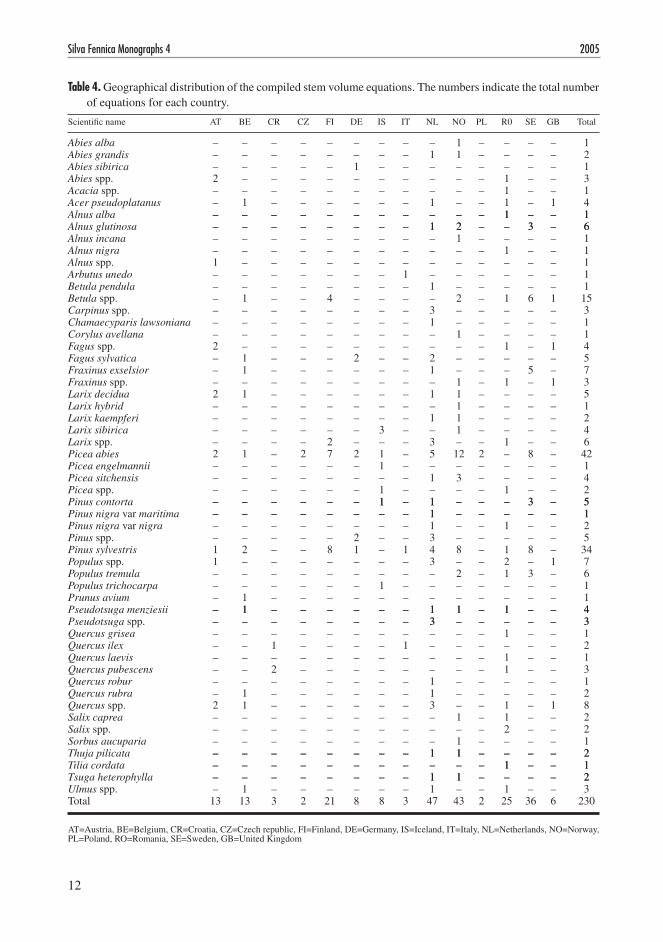
The total number of the compiled stem volume equations was �30 (App. B and c), and they cov-ered 55 tree species altogether (Table 4). Most of the European countries have already developed
stem volume equations mainly for the planning of the use of forest resources. However, there is no straightforward, commonly accepted defini-tion for stem volume in Europe. In general, the volume of stemwood extending from root collar up to the top of the stems is accounted in the equations developed in the Nordic countries. For some of the reviewed regressions, the stem is the part of the main trunk up to a minimum diameter of 7 cm (it is usually called the merchantable volume) while some authors have not reported definition of the stem related to their equations.
1�
Silva Fennica Monographs 4 2005
Table 4. Geographical distribution of the compiled stem volume equations. The numbers indicate the total number of equations for each country.
Scientific name AT BE cR cZ FI DE IS IT Nl NO Pl R0 SE GB Total
Abies alba – – – – – – – – – 1 – – – – 1Abies grandis – – – – – – – – 1 1 – – – – �Abies sibirica – – – – – 1 – – – – – – – – 1Abies spp. � – – – – – – – – – – 1 – – 3Acacia spp. – – – – – – – – – – – 1 – – 1Acer pseudoplatanus – 1 – – – – – – 1 – – 1 – 1 4Alnus alba – – – – – – – – – – – 1 – – 1– – – – – – – – – – – 1 – – 1Alnus glutinosa – – – – – – – – 1 � – – 3 – 6– – – – – – – – 1 � – – 3 – 6Alnus incana – – – – – – – – – 1 – – – – 1Alnus nigra – – – – – – – – – – – 1 – – 1Alnus spp. 1 – – – – – – – – – – – – – 1Arbutus unedo – – – – – – – 1 – – – – – – 1Betula pendula – – – – – – – – 1 – – – – – 1Betula spp. – 1 – – 4 – – – – � – 1 6 1 15Carpinus spp. – – – – – – – – 3 – – – – – 3Chamaecyparis lawsoniana – – – – – – – – 1 – – – – – 1Corylus avellana – – – – – – – – – 1 – – – – 1Fagus spp. � – – – – – – – – – – 1 – 1 4Fagus sylvatica – 1 – – – � – – � – – – – – 5Fraxinus exselsior – 1 – – – – – – 1 – – – 5 – 7Fraxinus spp. – – – – – – – – – 1 – 1 – 1 3Larix decidua � 1 – – – – – – 1 1 – – – – 5Larix hybrid – – – – – – – – – 1 – – – – 1Larix kaempferi – – – – – – – – 1 1 – – – – �Larix sibirica – – – – – – 3 – – 1 – – – – 4Larix spp. – – – – � – – – 3 – – 1 – – 6Picea abies � 1 – � 7 � 1 – 5 1� � – 8 – 4�Picea engelmannii – – – – – – 1 – – – – – – – 1Picea sitchensis – – – – – – – – 1 3 – – – – 4Picea spp. – – – – – – 1 – – – – 1 – – �Pinus contorta – – – – – – 1 – 1 – – – 3 – 5– – – – – – 1 – 1 – – – 3 – 5Pinus nigra var maritima – – – – – – – – 1 – – – – – 1– – – – – – – – 1 – – – – – 1Pinus nigra var nigra – – – – – – – – 1 – – 1 – – �Pinus spp. – – – – – � – – 3 – – – – – 5Pinus sylvestris 1 � – – 8 1 – 1 4 8 – 1 8 – 34Populus spp. 1 – – – – – – – 3 – – � – 1 7Populus tremula – – – – – – – – – � – 1 3 – 6Populus trichocarpa – – – – – – 1 – – – – – – – 1Prunus avium – 1 – – – – – – – – – – – – 1Pseudotsuga menziesii – 1 – – – – – – 1 1 – 1 – – 4– 1 – – – – – – 1 1 – 1 – – 4Pseudotsuga spp. – – – – – – – – 3 – – – – – 3– – – – – – – – 3 – – – – – 3Quercus grisea – – – – – – – – – – – 1 – – 1Quercus ilex – – 1 – – – – 1 – – – – – – �Quercus laevis – – – – – – – – – – – 1 – – 1Quercus pubescens – – � – – – – – – – – 1 – – 3Quercus robur – – – – – – – – 1 – – – – – 1Quercus rubra – 1 – – – – – – 1 – – – – – �Quercus spp. � 1 – – – – – – 3 – – 1 – 1 8Salix caprea – – – – – – – – – 1 – 1 – – �Salix spp. – – – – – – – – – – – � – – �Sorbus aucuparia – – – – – – – – – 1 – – – – 1Thuja pilicata – – – – – – – – 1 1 – – – – �– – – – – – – – 1 1 – – – – �Tilia cordata – – – – – – – – – – – 1 – – 1– – – – – – – – – – – 1 – – 1Tsuga heterophylla – – – – – – – – 1 1 – – – – �– – – – – – – – 1 1 – – – – �Ulmus spp. – 1 – – – – – – 1 – – 1 – – 3Total 13 13 3 � �1 8 8 3 47 43 � �5 36 6 �30
AT=Austria, BE=Belgium, cR=croatia, cZ=czech republic, FI=Finland, DE=Germany, IS=Iceland, IT=Italy, Nl=Netherlands, NO=Norway, Pl=Poland, RO=Romania, SE=Sweden, GB=United Kingdom

13
Zianis, Muukkonen, Mäkipää and Mencuccini Biomass and Stem Volume Equations for Tree Species in Europe
If the definition of the stem volume is reported in the original paper, it is indicated in the comment field of the appendix table (Appendix B).
The major part of the stem volume regressions was for coniferous tree species (Table 4). Forty-two equations were reported for Norway spruce (Picea abies (l.) Karst.) and 34 for Scots pine (Pinus sylvestris l.), from which more than half were built for Scandinavian countries. For the broadleaved tree species within the genera of Betula, Fagus, and Quercus the number of avail-able equations were 16, 9, and 18, respectively.
Most of the stem volume equations were based on a sample size of several hundred or a few thou-sand felled trees (Fig. 1b). Only three equations were based on a sample size of more than 5000 trees. In 97 of the equations the number of sample trees was not reported.
In almost every of the compiled stem volume equations the independent variables were D and/or H or various mathematical combinations of these (Appendix c). However, in three equa-tions the formula used to fit the tree-scale data was solely based on D and was a simple power func-tion (simple allometric equation). More than two parameters were incorporated into the formulae of �1� stem volume regressions, and 18 equations included six parameters. The number of the sam-
pled trees (from which the empirical stem volume regressions were obtained) varied from five to more than 7446 (Appendix B). The range of diam-eters of the sampled trees varied between equa-tions and for 1�5 of the compiled stem volume equations the range was not reported. In all the compiled equations the coefficient of determina-tion was more than 0.58 irrespective of species, location, D range, site conditions, etc.
Predicted stem volume estimates varied accord-ing to the applied equation (Fig. 3 and Fig. 4). For example, the stem volume of a beech tree with a diameter of 40 cm varies between 1.1 and �.� m3 (Fig. 3). On the other hand, all stem volume equations of e.g. Scots pine produced relatively consistent stem volume estimates. The equation reported by Schelhaas et al. (�00�) and one of the equations published by laasasenaho (198�) seemed to deviate from the others (Fig. 4). However, laasasenaho (198�) reported two other equations which had different form or more explanatory variables (height in addition to dbh), and they gave consistent predictions with the models of other authors.
0
1
2
3
4
0 10 20 30 40 50 60D (cm)
Ste
m v
olum
e (m
3 )
a
bc
d
Fagus sylvatica
a (Pellinen 1986)b (Dagnelie et al.1985)c (Dik 1984)d (De Vries 1961)
Fig. 3. Predicted stem volume of Fagus sylvatica as a function of tree diameter (D). The volume equa-tions are presented in Appendices B and c.
Fig. 4. Predicted stem volume of Pinus sylvestris as a function of tree diameter (D). The volume equa-tions are presented in Appendices B and c.
0
1
2
0 10 20 30 40 50
D (cm)
Ste
m v
olum
e (m
3 )
Pinus sylvestris
a (Laasasenaho 1982; Equation 148)
b (Schelhaas et al. 2002)
a
b
14
Reliable methods of estimating forest biomass and carbon stocks as well as volume of the grow-ing stock at different spatial and temporal scales and for different biomes are needed. In national forest inventories, emphasis has been placed on the assessment of merchantable timber, and inventories provide highly accurate estimates of the growing stock (laitat et al. �000). The cur-rent need to assess changes in the forest carbon has arisen as a result of the climate convention and the Kyoto Protocol. In general, assessment of forest biomass and carbon stock is based on information on forest resources i.e. estimates of forested area and volume of the growing stock as reported by national forest inventories (liski and Kauppi �000). Reported volume estimates are multiplied with simple biomass expansion fac-tors and/or conversion factors to obtain biomass estimates.
In national inventories, the volume of the grow-ing stock is estimated with the help of volume equations. The results of this study show that representative volume equations are available for major tree species in Europe, since volume equa-tions are developed for different vegetation zones and most of the equations are based on a rela-tively high number of sampled trees. However, the volume equations vary in terms of the dimensions accounted for (merchantable stem volume only or unmerchantable included), and the estimates obtained with different equations cannot be com-pared or aggregated, and they cannot be converted to biomass estimates by just using a single bio-mass expansion value. The differences were the most evident with tree species that had irregular branching patterns (e.g. beech), whereas volume equations of e.g. Scots pine were more consistent. The inconsistency of the different volume equa-tions applied to national forest inventories was also reported by Köhl et al. (1997). As national estimates of the volume of the growing stock are converted to biomass estimates, the applicability of the biomass expansion factors to the applied
volume equation needs to be evaluated to avoid highly biased biomass estimates.
Reliability of the national carbon inventories can be improved by applying biomass equations directly to tree-scale measurements of diameter (D) at sampled plots of forest inventories (Jal-kanen et al. �005). consequently, the additional source of error introduced by conversion or expansion factors can be avoided. The compiled database on biomass equations provides a basis for the selection of the applicable biomass equa-tion when representative national equations are not available. The database can be also used as a source of reference for the development of local equations. Since the number of sampled trees used for the development of the biomass equations seemed to be relatively small, it is necessary to use several equations rather than only one in order to obtain unbiased predictions.
The analysis of the collected information showed that both species coverage and the spa-tial distribution of the equations is limited. The vast majority of the models were developed for coniferous tree species growing in northern and central European forest ecosystems. Only a small number of biomass and stem volume regressions were collected for tree species in the eastern and southern parts of Europe (Tables 3 and 4). A rather limited number of equations for the estimation of root biomass has been compiled so far, indicating that a more extensive survey should take place and that more root biomass datasets should be collected across Europe. In a similar study conducted in Australia, Snowdon et al. (�000) stressed that more root biomass studies are needed and suggested that fractal geometry could be a promising tool to overcome the practical problems arising from the destructive sampling of belowground tree biomass. Ter-Mikaelian and Korzukhin (1997) reported no equations for esti-mating the root biomass of tree species growing in the USA.
Most of the collected equations lack information
4 Discussion

15
Zianis, Muukkonen, Mäkipää and Mencuccini Biomass and Stem Volume Equations for Tree Species in Europe
on the error estimates of the empirical parameters. According to Keith et al. (�000), the main sources of error in implementing allometric regressions could occur at the treescale and when biomass estimates are extrapolated from plot to regional scale (see also Satoo and Madgwick 198�). It should be noticed that when a logarithmic or any other transformation is applied to the raw data, biomass and stem volume predictions are biased (Baskerville 197�, Sprugel 1983). Mathematical formulae for correcting bias provide accurate estimates even though assumptions about the dis-tribution of statistical errors must be made. The inherent bias arising from data transformation could be eliminated if iterative procedures were to be applied to the data (for a more detailed discussion see Payandeh 1981).
Biased predictions may also be obtained when the sum of biomass estimates (developed for different tree components i.e., stem, crown and roots) does not match the predictions derived from the total biomass equation (what is called the additivity problem). Parresol (�001) provided statistical methods to account for this bias while Snowdon et al. (�000) reported that the additivity problem does not appear when allometric equa-tions are developed from non-transformed data. Another statistical problem is caused by colline-arity or multicollinearity, where the independent variables in a regression analysis are themselves correlated (Ott 1993). Thus, the value of the coefficient of determination in stem volume and biomass equations (with more than one independ-ent variable) may not be a reliable criterion for the choice of the best-fitting equation, and biased predictions may be obtained when this problem is not taken into account. However, the collinearity problem is seldom mentioned in original papers, where more often than not, diameter and height are the independent variables in estimating either stem volume or tree biomass.
The equations presented in this review can be used for national biomass and carbon invento-ries, for ecological studies, for validating theo-retical models and for planning the use of forest resources. Since the original biomass studies may have been conducted for very specific purposes, following different sampling procedures and per-haps atypical stand structures, the applicability of an equation to its intended purpose needs to be evaluated in terms of the geographical distribu-tion of the sampled population, the number of sampled trees, the range of dimensions (D, H) of sampled trees, accounted dimensions and applied definitions.
Pooled equations based on raw data collected from wide geographical areas may also provide a promising alternative to estimate biomass changes at the landscape scale Wirth et al. �004). The empirical models reviewed in this article may also be used in order to build generalised stem volume and biomass equations for different spe-cies and different tree components (see Pastor et al. 1983/1984 for American species and Zianis and Mencuccini �003 for the genus Fagus), to develop BEF for tree species across Europe (lehtonen et al. �004) and to validate process-based models of forest productivity.

16
Baskerville, G.l. 197�. Use of logarithmic regression in the estimation of plant biomass. canadian Jour-nal of Forestry �: 49–53.
Brown, S. 1997. Estimating biomass and biomass change of tropical forests, a premier. FAO For-estry Paper 134.
Bruce, D. & Schumacher, F.X. 1950. Forest mensu-ration. McGraw-Hill Book company, Inc. New York. 483 p.
clark, D.A., Brown, S., Kicklighter, D.W., chambers, J.Q., R, T.J. & Ni, J. �001. Measuring net primary production in forests: concepts and field methods. Ecological Applications 11(�): 356–370.
Drake, J.B., Dubayah, R.O., Knox, R.G., clark, D.B. & Blair, J.B. �00�. Sensitivity of large-footprint lidar to canopy structure and biomass in a neotropical rainforest. Remote Sensing of Environment 81: 378–39�.
Eamus, D., McGuinness, K. & Burrows, W. �000. Review of allometric relationships for estimat-ing woody biomass for Queensland, the Northern Territory and Western Australia. National carbon Accounting System Technical Report 5A. Austral-ian Greenhouse Office, canberra. 56 p.
Hall, D.O. 1997. Biomass energy in industrialised countries – a view of the future. Forest Ecology and Management 91: 17–45.
IPcc, �003. Report on good practice guidance for land use, land-use change and forestry. IPcc National Greenhouse Gas Inventories Programme http://www.ipcc-nggip.iges.or.jp/public/gpglulucf/gpglu-lucf.htm., Japan.
Jalkanen, A., Mäkipää, R., Ståhl, G., lehtonen, A. & Petersson, H. �005. Estimation of biomass stock of trees in Sweden: comparison of biomass equa-tions and age-dependent biomass expansion fac-tors. Annals of Forest Science 6� (In press)
Jenkins, J.c., chojnacky, D.c., Heath, l.S. & Bird-sey, R.A. �003. National-scale biomass estimators for United States tree species. Forest Science 49: 1�–35.
— , chojnacky, D.c., Heath, l.S. & Birdsey, R.A. �004. comprehensive database of diameter-based biomass regressions for North American tree spe-cies. Gen. Tech. Rep. NE-319. US Forest Service. 45 p.
Keith, H., Barrett, D. & Keenan, R. �000. Review of allometric relationships for estimating woody bio-mass for New South Wales, the Australian capital Territory, Victoria, Tasmania, and South Australia. National carbon Accounting System Technical Report 5B. Australian Greenhouse Office, can-berra. 114 p.
Köhl, M., Päivinen, R., Traub, B. & Miina, S. 1997. comparative study. In: Study on European forestry information and communication system. Reports on forest inventory and survey systems �. European commission. p. 1�65–13��.
laitat, E., Karjalainen, T., loustau, D. & lindner, M. �000. Towards an integrated scientific approach for carbon accounting in forestry. Biotechnol-ogy, Agronomy, Society and Environment 4: �41–�51.
lehtonen, A., Mäkipää, R., Heikkinen, J., Sievänen, R. & liski, J. �004. Biomass expansion factors (BEFs) for Scots pine, Norway spruce and birch according to stand age for boreal forests. Forest Ecology and Management 188: �11–��4.
liski, J. & Kauppi, P. �000. carbon cycle and bio-mass. In: FAO (ed.). Forest resources of Europe, cIS, North America, Australia, Japan and New Zealand (industrialized temperate/boreal coun-tries). UN-EcE/FAO contribution to the Global Forest Resources Assessment �000, Main Report (in press). United Nations, New York and Geneva. p. 155–171.
löwe, H., Seufert, G. & Raes, F. �000. comparison of methods used within member states for estimating cO� emissions and sinks to UNFccc and UE monitoring mechanism: forest and other wooded land. Biotechnology, Agronomy, Society and Envi-ronment 4: 315–319.
References
17
Zianis, Muukkonen, Mäkipää and Mencuccini Biomass and Stem Volume Equations for Tree Species in Europe
Marklund, l.G. 1987. Biomass functions for Norway spruce (Picea abies (l.) Karst.) in Sweden. Sveriges lantbruksuniversitet, Institutionen för skogstaxer-ing, Rapport 43. 1�7 p.
— 1988. Biomassafunktioner för tall, gran och björk i Sverige. Sveriges lantbruksuniversitet, Institutio-nen för skogstaxering, Rapport 45. 73 p.
Montes, N., Gauquelin, T., Badri, W., Bertaudiere, V. & Zaoui, E.H. �000. A non-destructive method for estimating above-ground forest biomass in threat-ened woodlands. Forest Ecology and Management 130: 37–46.
Ott, R.l. 1993. An introduction to statistical methods and data analysis. Duxbury press, california. 13� p.
Parresol, R.B. �001. Additivity of nonlinear biomass equations. canadian Journal of Forest Research 31: 865–878.
Pastor, J., Aber, J.D. & Melillo, J.M. 1983/1984. Biomass prediction using generalized allometric regerssions for some northeast tree species. Forest Ecology and Management 7: �65–�74.
Payandeh, B. 1981. choosing regression models for biomass prediction equations. The Forestry chroni-cle 57: �30–�3�.
Santantonio, D., Hermann, R.K. & Overton, W.S. 1977. Root biomass studies in forest ecosystems. Pedo-biologia 17: 1–31.
Satoo, T. & Madgwick, H.A.I. 198�. Forest biomass. Kluwer Academic Publishers Group, london. 160 p.
Snowdon, P., Eamus, D., Gibbons, P., Khanna, P.K., Keith, H., Raison, R.J. & Kirschbaum, M.U.F. �000. Synthesis of allometrics, revieew of root biomass and design of future woody biomass sampling strategies. National carbon Accounting System Technical Report 17. Australian Green-house Office, canberra. 114 p.
Sprugel, D.G. 1983. correcting for bias in log-trans-formed allometric equations. Ecology 64: �09–�10.
Ter-Mikaelian, M.T. & Korzukhin, M.D. 1997. Biomass equations for sixty-five North American tree spe-cies. Forest Ecology and Management 97: 1–�4.
Tritton, l.M. & Hornbeck, J.W. 198�. Biomass equa-tions for major tree species of the Northeast U.S. Department of Agriculture, Northeastern Forest Experiment Station, General Technical Report NE-69. 46 p.
Wirth, c., Schumacher, J. & Schulze, E.-D. �004. Generic biomass functions for Norway spruce in central Europe – a meta-analysis approach toward prediction and uncertainty estimation. Tree Physi-ology �4: 1�1–139.
Zianis, D. & Mencuccini, M. �003. Aboveground bio-mass relationship for beech (Fagus moesiaca cz.) trees in Vermio Mountain, Northern Greece, and generalised equations for Fagus spp. Annals of Forest Science 60: 439–448.
— �004. On simplifying allometric analyses of forest biomass. Forest Ecology and Management 187: 311–33�.
Total of 33 references
18
Silva Fennica Monographs 4 2005
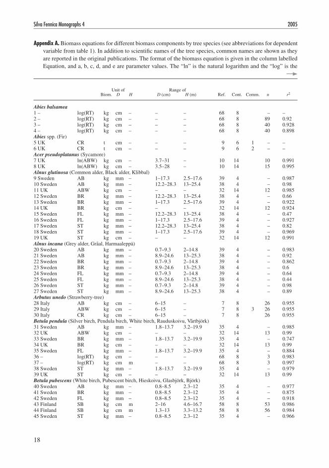
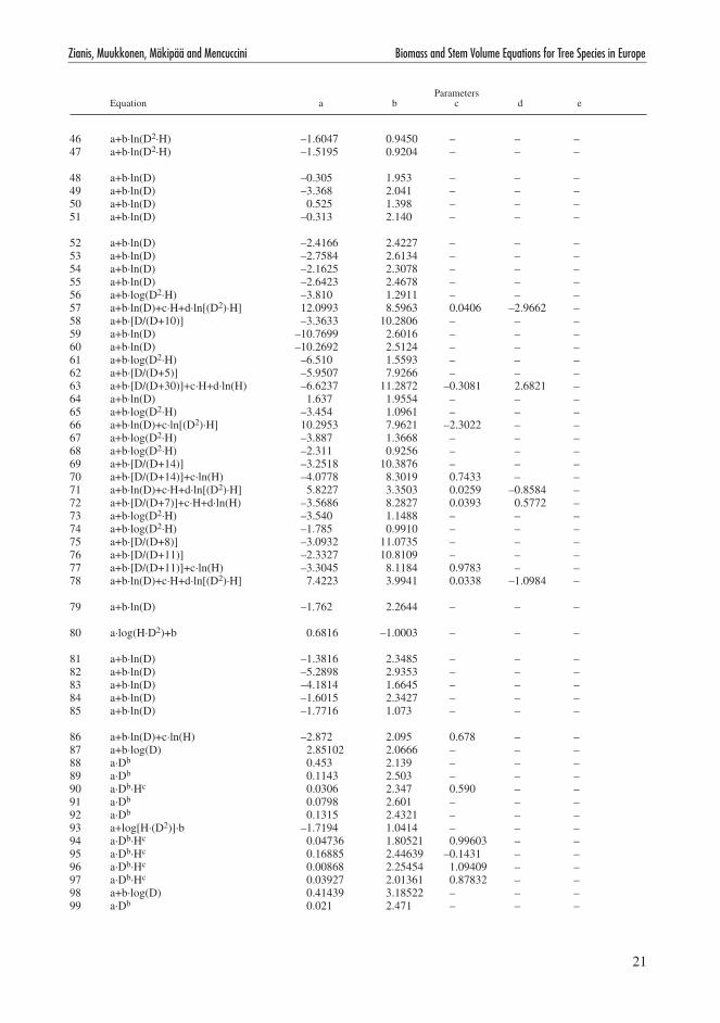
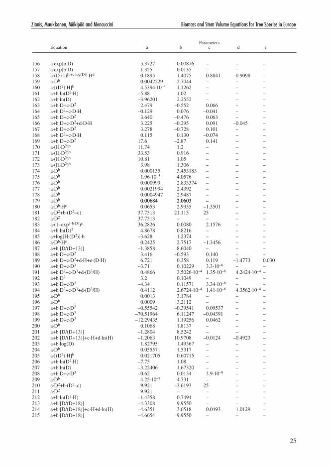
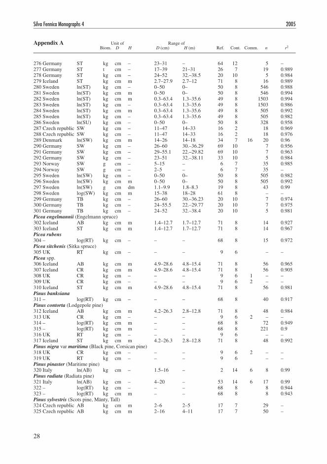
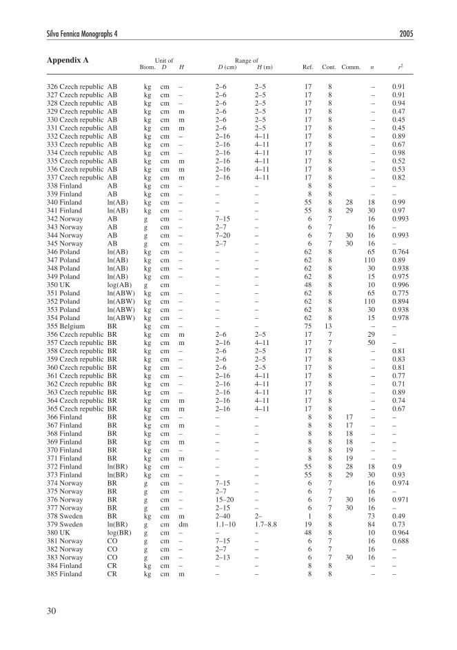
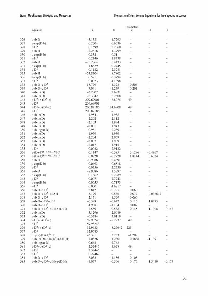
Appendix A. Biomass equations for different biomass components by tree species (see abbreviations for dependent variable from table 1). In addition to scientific names of the tree species, common names are shown as they are reported in the original publications. The format of the biomass equation is given in the column labelled Equation, and a, b, c, d, and e are parameter values. The “ln” is the natural logarithm and the “log” is the
Unit of Range of Biom. D H D (cm) H (m) Ref. cont. comm. n r�
Abies balsamea1 – log(RT) kg cm – – – 68 8 – –� – log(RT) kg cm – – – 68 8 89 0.9�3 – log(RT) kg cm – – – 68 8 40 0.9�84 – log(RT) kg cm – – – 68 8 40 0.898Abies spp. (Fir)5 UK cR t cm – – – 9 6 1 – –6 UK cR t cm – – – 9 6 � – –Acer pseudoplatanus (Sycamore)7 UK ln(ABW) kg cm – 3.7–31 – 10 14 10 0.9918 UK ln(ABW) kg cm – 3.5–�8 – 10 14 15 0.995Alnus glutinosa (common alder, Black alder, Klibbal)9 Sweden AB kg mm – 1–17.3 �.5–17.6 39 4 – 0.98710 Sweden AB kg mm – 1�.�–�8.3 13–�5.4 38 4 – 0.9811 UK ABW kg cm – – – 3� 14 1� 0.9851� Sweden BR kg mm – 1�.�–�8.3 13–�5.4 38 4 – 0.6613 Sweden BR kg mm – 1–17.3 �.5–17.6 39 4 – 0.9��14 UK BR kg cm – – – 3� 14 1� 0.9�415 Sweden Fl kg mm – 1�.�–�8.3 13–�5.4 38 4 – 0.4716 Sweden Fl kg mm – 1–17.3 �.5–17.6 39 4 – 0.9�717 Sweden ST kg mm – 1�.�–�8.3 13–�5.4 38 4 – 0.8�18 Sweden ST kg mm – 1–17.3 �.5–17.6 39 4 – 0.96919 UK ST kg cm – – – 3� 14 1� 0.991Alnus incana (Grey alder, Gråal, Harmaaleppä)�0 Sweden AB kg mm – 0.7–9.3 �–14.8 39 4 – 0.983�1 Sweden AB kg mm – 8.9–�4.6 13–�5.3 38 4 – 0.9��� Sweden BR kg mm – 0.7–9.3 �–14.8 39 4 – 0.86��3 Sweden BR kg mm – 8.9–�4.6 13–�5.3 38 4 – 0.6�4 Sweden Fl kg mm – 0.7–9.3 �–14.8 39 4 – 0.64�5 Sweden Fl kg mm – 8.9–�4.6 13–�5.3 38 4 – 0.44�6 Sweden ST kg mm – 0.7–9.3 �–14.8 39 4 – 0.98�7 Sweden ST kg mm – 8.9–�4.6 13–�5.3 38 4 – 0.89Arbutus unedo (Strawberry-tree)�8 Italy AB kg cm – 6–15 – 7 8 �6 0.955�9 Italy ABW kg cm – 6–15 – 7 8 3 �6 0.95530 Italy cR kg cm – 6–15 – 7 8 �6 0.955Betula pendula (Silver birch, Pendula birch, White birch, Rauduskoivu, Vårtbjörk)31 Sweden AB kg mm – 1.8–13.7 3.�–19.9 35 4 – 0.9853� UK ABW kg cm – – – 3� 14 13 0.9933 Sweden BR kg mm – 1.8–13.7 3.�–19.9 35 4 – 0.74734 UK BR kg cm – – – 3� 14 13 0.9935 Sweden Fl kg mm – 1.8–13.7 3.�–19.9 35 4 – 0.88436 – log(RT) kg cm – – – 68 8 3 0.98337 – log(RT) kg cm m – – 68 8 3 0.99738 Sweden ST kg mm – 1.8–13.7 3.�–19.9 35 4 – 0.97939 UK ST kg cm – – – 3� 14 13 0.99Betula pubescens (White birch, Pubescent birch, Hieskoivu, Glasbjörk, Björk)40 Sweden AB kg mm – 0.8–8.5 �.3–1� 35 4 – 0.97741 Sweden BR kg mm – 0.8–8.5 �.3–1� 35 4 – 0.8754� Sweden Fl kg mm – 0.8–8.5 �.3–1� 35 4 – 0.91843 Finland SB kg cm m �–16 4.6–16.7 58 8 53 0.98644 Finland SB kg cm m 1.3–13 3.3–13.� 58 8 56 0.98445 Sweden ST kg mm – 0.8–8.5 �.3–1� 35 4 – 0.966

19
Zianis, Muukkonen, Mäkipää and Mencuccini Biomass and Stem Volume Equations for Tree Species in Europe
10-based logarithm. Number of sampled trees (n), coefficients of determination (r�), and range of diameter (D) and height (H) of sampled trees are reported when available in the original article. References (Ref.) to the original papers according to author as well as the contact (cont.) person who submitted the equation to this database are given at the end of the table. In the comments column (comm.) occur some comments about the particular equation.
Parameters Equation a b c d e
1 a·log(D)+b �.445� –1.7143 – – –� a·log(D)+b �.45 0.681 – – –3 a·log(D)+b �.00�7 0.06�9 – – –4 a·log(D)+b �.4613 –0.40�3 – – –
5 a·Db 5.�193·10–4 1.459 – – –6 a+b·Dc 0.00607�� 9.58·10–6 �.5578 – –
7 a+b·ln(D) –�.7606 �.5189 – – –8 a+b·ln(D) –�.7018 �.5751 – – –
9 a·Db 0.00079 �.�8546 – – –10 a·Db 0.003090 �.0��1�6 – – –11 a·Db 0.0859 �.3537 – – –1� a·Db 0.000003 �.880598 – – –13 a·Db 0.0000006 3.�8106 – – –14 a·Db 0.0146 �.5191 – – –15 a·Db 0.000003 �.547045 – – –16 a·Db 0.00�39 1.3�535 – – –17 a·Db 0.005609 1.888345 – – –18 a·Db 0.00119 �.17�47 – – –19 a·Db 0.0841 �.4501 – – –
�0 a·Db 0.00030 �.4�847 – – –�1 a·Db 0.000499 �.33759� – – –�� a·Db 0.00001 �.65455 – – –�3 a·Db 0.000100 �.�97058 – – –�4 a·Db 0.00001 �.44406 – – –�5 a·Db 0.000076 �.0�604 – – –�6 a·Db 0.000�9 �.401�8 – – –�7 a·Db 0.000368 �.335763 – – –
�8 a+b·D� –�.7563 0.3045 – – –�9 a+b·D� –�.8816 0.�639 – – –30 a+b·D� 0.1�53 0.040617 – – –
31 a·Db 0.00087 �.�8639 – – –3� a·Db 0.�511 �.�9 – – –33 a·Db 0.0000� �.63001 – – –34 a·Db 0.074� �.�4 – – –35 a·Db 0.00371 1.11993 – – –36 a·log(D)+b �.3547 –1.3 – – –37 a·log(H·D�)+b 0.9308 –1.8 – – –38 a·Db 0.00080 �.�8�44 – – –39 a·Db 0.193 �.�5 – – –
40 a·Db 0.000�9 �.50038 – – –41 a·Db 0.00004 �.5�978 – – –4� a·Db 0.00090 1.47663 – – –43 a+b·ln(D�·H) –�.1909 0.8808 – – –44 a+b·ln(D�·H) –�.0706 0.794� – – –45 a·Db 0.000�0 �.5430� – – –

�0
Silva Fennica Monographs 4 2005
46 Finland SW kg cm m �–16 4.6–16.7 58 8 53 0.99447 Finland SW kg cm m 1.3–13 3.3–13.� 58 8 56 0.994Betula pubescens ssp. czerepanovii (Mountain birch)48 Finland ln(BR) g mm – – – 7� 8 �0 0.83649 Finland ln(DB) g mm – – – 7� 8 �0 0.6��50 Finland ln(Fl) g mm – – – 7� 8 �0 0.8�951 Finland ln(ST) g mm – – – 7� 8 �0 0.98Betula spp. (Birch, Koivu, Björk)5� UK ln(ABW) kg cm – �.9–30 – 10 14 �7 0.98553 UK ln(ABW) kg cm – �.9–�6 – 10 14 15 0.98454 UK ln(ABW) kg cm – 3.3–16 – 10 14 16 0.98455 UK ln(ABW) kg cm – 3.5–�3 – 10 14 15 0.98756 Finland BR kg cm m 9–�8 13–��.4 57 8 �0 0.90157 Sweden ln(BR) g cm dm 0.9–9.8 1.8–9.� 19 8 66 0.8858 Sweden ln(BR) kg cm – 0–35 0– 50 8 4 �35 0.9�459 Finland ln(cR) kg mm – – – �9 8 – 0.83960 Finland ln(cR) kg mm – – – �9 8 – 0.83861 Finland DB kg cm m 9.0–�8 13–��.4 57 8 �0 0.�676� Sweden ln(DB) kg cm – 0–35 0– 50 8 �1� 0.60563 Sweden ln(DB) kg cm m 0–35 0– 50 8 �1� 0.6�164 Sweden ln(DB) g cm – 0.9–9.8 18–9� 19 8 61 0.5665 Finland Fl kg cm m 9–�8 13–��.4 57 8 �0 0.90666 Sweden ln(Fl) g cm dm 0.9–9.8 1.8–9.� 19 8 14 0.9�67 Finland RT kg cm m 9–�8 13–��.4 57 8 5 �0 0.99468 Finland SB kg cm m 9–�8 13–��.4 57 8 �0 0.96669 Sweden ln(SB) kg cm – 0–35 0– 50 8 �1� 0.94770 Sweden ln(SB) kg cm m 0–35 0– 50 8 �1� 0.95871 Sweden ln(SB) g cm dm 0.9–9.8 1.8–9.� 19 8 66 0.917� Sweden ln(ST) kg cm m 0–35 0– 50 8 �40 0.99�73 Finland SU kg cm m 9–�8 13–��.4 57 8 �0 0.9674 Finland SW kg cm m 9–�8 13–��.4 57 8 �0 0.9975 Sweden ln(SW) kg cm – 0–35 0– 50 8 �40 0.98�76 Sweden ln(SW) kg cm – 0–35 0– 50 8 �1� 0.9777 Sweden ln(SW) kg cm m 0–35 0– 50 8 �1� 0.9978 Sweden ln(SW) g cm dm 0.9–9.8 1.8–9.� 19 8 66 0.99Eucalyptus spp. (Eucalypt)79 Italy ln(AB) kg cm – 4–�5 – 53 14 6 �� 0.99Fagus crenata80 – log(RT) kg cm m – – 68 8 7 0.969Fagus moesiaca (Beech, Oxia)81 Greece ln(AB) kg cm – 5.4–41 9.�–�8 76 14 16 0.998� Greece ln(BR) kg cm – 5.4–41 9.�–�8 76 14 16 0.9783 Greece ln(Fl) kg cm – 5.4–41 9.�–�8 76 14 16 0.984 Greece ln(ST) kg cm – 5.4–41 9.�–�8 76 14 16 0.9885 Greece ln(SU) kg cm – 5.4–41 9.�–�8 76 14 7 16 0.78Fagus sylvatica (Beech, European beech, Hêtres, Rotbuche)86 Austria ln(AB) kg cm m – – 31 3 4� 0.99787 Belgium log(AB) g cm – 35–78.8 – �3 1� 6 0.99588 czech republic AB kg cm – 5.7–6�.1 9.�–33.9 15 � �0 0.97489 Germany AB kg cm – – – 65 4 – –90 Netherlands AB kg cm m – – 5 8 38 0.99191 Netherlands AB kg cm – – – 5 8 38 0.9889� Spain AB kg cm – 4–34.5 6.1–18.4 67 14 7 0.9893 Sweden log(AB) kg cm m 1�–64 11–�9 61 8 – –94 Italy ABW kg cm m – – 11 8 8 – 0.99395 Italy ABW kg cm m – – 11 8 9 – 0.98896 Italy ABW kg cm m – – 11 8 10 – 0.99197 Italy ABW kg cm m – – 11 8 – 0.99598 Belgium log(BR) g cm – 35–78.8 – �3 1� 6 0.98199 czech republic BR kg cm – 5.7–6�.1 9.�–33.9 15 � �0 0.806
Appendix A Unit of Range of Biom. D H D (cm) H (m) Ref. cont. comm. n r�
�1
Zianis, Muukkonen, Mäkipää and Mencuccini Biomass and Stem Volume Equations for Tree Species in Europe
46 a+b·ln(D�·H) –1.6047 0.9450 – – –47 a+b·ln(D�·H) –1.5195 0.9�04 – – –
48 a+b·ln(D) –0.305 1.953 – – –49 a+b·ln(D) –3.368 �.041 – – –50 a+b·ln(D) 0.5�5 1.398 – – –51 a+b·ln(D) –0.313 �.140 – – –
5� a+b·ln(D) –�.4166 �.4��7 – – –53 a+b·ln(D) –�.7584 �.6134 – – –54 a+b·ln(D) –�.16�5 �.3078 – – –55 a+b·ln(D) –�.64�3 �.4678 – – –56 a+b·log(D�·H) –3.810 1.�911 – – –57 a+b·ln(D)+c·H+d·ln[(D�)·H] 1�.0993 8.5963 0.0406 –�.966� –58 a+b·[D/(D+10)] –3.3633 10.�806 – – –59 a+b·ln(D) –10.7699 �.6016 – – –60 a+b·ln(D) –10.�69� �.51�4 – – –61 a+b·log(D�·H) –6.510 1.5593 – – –6� a+b·[D/(D+5)] –5.9507 7.9�66 – – –63 a+b·[D/(D+30)]+c·H+d·ln(H) –6.6�37 11.�87� –0.3081 �.68�1 –64 a+b·ln(D) 1.637 1.9554 – – –65 a+b·log(D�·H) –3.454 1.0961 – – –66 a+b·ln(D)+c·ln[(D�)·H] 10.�953 7.96�1 –�.30�� – –67 a+b·log(D�·H) –3.887 1.3668 – – –68 a+b·log(D�·H) –�.311 0.9�56 – – –69 a+b·[D/(D+14)] –3.�518 10.3876 – – –70 a+b·[D/(D+14)]+c·ln(H) –4.0778 8.3019 0.7433 – –71 a+b·ln(D)+c·H+d·ln[(D�)·H] 5.8��7 3.3503 0.0�59 –0.8584 –7� a+b·[D/(D+7)]+c·H+d·ln(H) –3.5686 8.�8�7 0.0393 0.577� –73 a+b·log(D�·H) –3.540 1.1488 – – –74 a+b·log(D�·H) –1.785 0.9910 – – –75 a+b·[D/(D+8)] –3.093� 11.0735 – – –76 a+b·[D/(D+11)] –�.33�7 10.8109 – – –77 a+b·[D/(D+11)]+c·ln(H) –3.3045 8.1184 0.9783 – –78 a+b·ln(D)+c·H+d·ln[(D�)·H] 7.4��3 3.9941 0.0338 –1.0984 –
79 a+b·ln(D) –1.76� �.�644 – – –
80 a·log(H·D�)+b 0.6816 –1.0003 – – –
81 a+b·ln(D) –1.3816 �.3485 – – –8� a+b·ln(D) –5.�898 �.9353 – – –83 a+b·ln(D) –4.1814 1.6645 – – –84 a+b·ln(D) –1.6015 �.34�7 – – –85 a+b·ln(D) –1.7716 1.073 – – –
86 a+b·ln(D)+c·ln(H) –�.87� �.095 0.678 – –87 a+b·log(D) �.8510� �.0666 – – –88 a·Db 0.453 �.139 – – –89 a·Db 0.1143 �.503 – – –90 a·Db·Hc 0.0306 �.347 0.590 – –91 a·Db 0.0798 �.601 – – –9� a·Db 0.1315 �.43�1 – – –93 a+log[H·(D�)]·b –1.7194 1.0414 – – –94 a·Db·Hc 0.04736 1.805�1 0.99603 – –95 a·Db·Hc 0.16885 �.44639 –0.1431 – –96 a·Db·Hc 0.00868 �.�5454 1.09409 – –97 a·Db·Hc 0.039�7 �.01361 0.8783� – –98 a+b·log(D) 0.41439 3.185�� – – –99 a·Db 0.0�1 �.471 – – –
Parameters Equation a b c d e

��
Silva Fennica Monographs 4 2005
100 France ln(BR) kg cm – – – 4� 14 �3 0.93101 Netherlands BR kg cm m – – 5 8 38 0.9�10� Netherlands BR kg cm – – – 5 8 38 0.916103 Spain BR kg cm – 4–34.5 6.1–18.4 67 14 7 0.89104 Sweden log(BR) kg cm m 1�–64 11–�9 61 8 – –105 Netherlands cR kg cm m – – 5 8 38 0.9�9106 Netherlands cR kg cm – – – 5 8 38 0.9�4107 UK cR t cm – – – 9 6 1 – –108 UK cR t cm – – – 9 6 1 – –109 France ln(Fl) kg cm – – – 4� 14 �3 0.95110 Italy Fl kg cm – – – 11 8 8 – 0.956111 Italy Fl kg cm m – – 11 8 – 0.96111� Netherlands Fl kg cm m – – 5 8 38 0.9�3113 Netherlands Fl kg cm – – – 5 8 38 0.906114 Spain Fl kg cm – 4–34.5 6.1–18.4 67 14 7 0.89115 France ln(Rc) kg cm – – – 4� 14 16 0.99116 France ln(RF) kg cm – – – 4� 14 16 0.94117 France ln(RS) kg cm – – – 4� 14 16 0.95118 France RT kg cm – – – 43 8 16 0.99119 France log(RT) kg cm – 3–�0 – �1 8 16 0.991�0 Germany log(RT) kg cm – 1�–47 – �1 8 8 0.981�1 Sweden log(RT) kg cm m 1�–64 11–�9 61 8 – –1�� France ln(SB) kg cm – – – 4� 14 �3 0.991�3 Sweden log(SB) kg cm m 1�–64 11–�9 61 8 – –1�4 czech republic ST kg cm – 5.7–6�.1 9.�–33.9 15 � �0 0.9541�5 Italy ST kg cm m – – 11 8 8 – 0.9881�6 Italy ST kg cm m – – 11 8 9 – 0.9951�7 Italy ST kg cm m – – 11 8 10 – 0.991�8 Italy ST kg cm m – – 11 8 – 0.9961�9 Netherlands ST kg cm m – – 5 8 38 0.996130 Netherlands ST kg cm – – – 5 8 38 0.979131 Spain ST kg cm – 4–34.5 6.1–18.4 67 14 7 0.9913� France ln(SW) kg cm – – – 4� 14 �3 0.99133 Sweden log(SW) kg cm m 1�–64 11–�9 61 8 – –Fraxinus excelsior (European ash)134 UK ln(ABW) kg cm – �.9–33 – 10 14 11 15 0.994135 UK ln(ABW) kg cm – 3–18 – 10 14 11 15 0.985Larix sibirica (Siberian larch)136 Iceland AB kg cm m 3.3–31.6 3–�0 71 8 44 0.99�137 Iceland ST kg cm m 3.3–31.6 3–�0 71 8 44 0.984Larix spp.138 UK cR t cm – – – 9 6 � – –Picea abies (Norway spruce, Kuusi, Gran, Fichte, Rødgran, Epicéa)139 Belgium AB g cm cm �.6–10 1.3–4.5 41 5 1� �3 0.98�140 czech republic AB kg cm m 1–11 �–9 18 7 13 55 –141 czech republic AB kg cm – 11–47 14–33 16 � 17 0.96714� czech republic AB kg cm m 11–47 14–33 16 � 17 0.971143 Denmark AB kg cm m 10–17 11–13 59 7 14 5 –144 Denmark AB kg cm m 1�–�0 11–14 59 7 15 10 –145 Finland AB kg cm – – – 8 8 – –146 Finland AB kg cm m – – 8 8 – –147 Germany AB kg cm – 17–39 – �6 1� 19 0.995148 Germany AB kg cm – 10.–�7.� – 64 1� 8 –149 Germany AB kg cm – 17–38 – 64 1� 9 –150 Germany AB kg cm – �3–31 – 64 1� 5 –151 Iceland AB kg cm m �.7–�7.9 �.7–1� 71 8 16 0.98115� Norway AB g cm – 5–15 – 6 7 35 0.993153 Norway AB g cm – �–5 – 6 7 35 –154 Sweden log(AB) kg cm m 15–38 18–�8 61 8 – –155 Belgium log(ABW) g cm – 16.–3�.3 – �4 1� 6 0.98�
Appendix A Unit of Range of Biom. D H D (cm) H (m) Ref. cont. comm. n r�

�3
Zianis, Muukkonen, Mäkipää and Mencuccini Biomass and Stem Volume Equations for Tree Species in Europe
100 a+b·ln(D) –6.�5�4 3.3�8 – – –101 a·Db·Hc 0.0114 3.68� –1.031 – –10� a·Db 0.00�0 3.�65 – – –103 a·Db 0.0317 �.3931 – – –104 a+log[H·(D�)]·b –3.�114 1.�481 – – –105 a·Db·Hc 0.0183 3.614 –1.078 – –106 a·Db 0.0031 3.161 – – –107 a·D� �.595·10–4 – – – –108 a+b·Dc 0.00686 1.9�·10–5 �.4658 – –109 a+b·ln(D) –4.8599 �.1935 – – –110 a·Db 0.00�95 �.43854 – – –111 a·Db·Hc 0.0�408 3.04567 –1.51571 – –11� a·Db·Hc 0.0167 �.951 –1.101 – –113 a+b·Dc 0.375 0.00�4 �.517 – –114 a·Db 0.0145 1.9531 – – –115 a+b·ln(D) –4.130� �.6099 – – –116 a+b·ln(D) –5.7948 �.1609 – – –117 a+b·ln(D) –5.4415 �.08� – – –118 a+b·ln(D) –3.8�19 �.538� – – –119 a+b·log(D) –1.66 �.54 – – –1�0 a+b·log(D) –� �.7 – – –1�1 a+log[H·(D�)]·b –�.8434 1.104 – – –1�� a+b·ln(D) –3.0741 �.0543 – – –1�3 a+log[H·(D�)]·b –�.4�79 0.8636 – – –1�4 a·Db 0.494 �.07 – – –1�5 a·Db·Hc 0.00519 1.49634 �.10419 – –1�6 a·Db·Hc 0.03638 �.15436 0.6587 – –1�7 a·Db·Hc 0.00�69 �.0�481 1.65�19 – –1�8 a·Db·Hc 0.00519 1.87511 1.�7�33 – –1�9 a·Db·Hc 0.0109 1.951 1.�6� – –130 a·Db 0.076� �.5�3 – – –131 a·Db 0.0894 �.4679 – – –13� a+b·ln(D) –�.0445 �.391� – – –133 a+log[H·(D�)]·b –1.6�19 0.9813 – – –
134 a+b·ln(D) –�.4598 �.488� – – –135 a+b·ln(D) –�.4718 �.5466 – – –
136 a·Db·Hc 0.1081 1.53 0.948� – –137 a·Db·Hc 0.0444 1.4793 1.�397 – –
138 a+b·Dc 0.00564 3.041·10–5 �.1058 – –
139 a+b·H+c·D² –5�0.7 –�.8 154.1 – –140 a·(D+1)[b+c·log(D)]·Hd 0.4�74 0.8674 1.0099 –0.�0�8 –141 a·Db 0.57669 1.964 – – –14� a·[(D�)·H]b 0.11975 0.81336 – – –143 a·D�H 0.0�155 – – – –144 a·D�H 0.01815 – – – –145 a+b·D+c·D² 19.018 –4.806 0.565 – –146 a+b·D²+c·(D²·H) 0.�57 0.187 0.010 – –147 a+b·D+c·D� –43.13 �.�5 0.45� – –148 a+b·D+c·D� –60.5570� 5.46558 0.�7567 – –149 a+b·D+c·D� –�83.17413 �6.3�334 –0.1�856 – –150 a+b·D+c·D� –14�.60881 13.63896 0.1�593 – –151 a·Db·Hc 0.�465 �.1� –0.167 – –15� a·D�+b·(D�–c) �00.3691 99.3609 �5 – –153 a·D� �00.3691 – – – –154 a+log[H·(D�)]·b –1.�908 0.891 – – –155 a+b·log(D) 1.81�98 �.51353 – – –
Parameters Equation a b c d e

�4
Silva Fennica Monographs 4 2005
156 Austria BR kg mm – 3.�–�0.7 – 60 1� 1� 0.731154 Austria BR kg mm – �.5–17.9 – 60 1� 1� 0.95158 czech republic BR kg cm m 1–11 �–9 18 7 13 55 –159 czech republic BR kg cm – 11–47 14–33 16 � �5 0.89�160 czech republic BR kg cm m 11–47 14–33 16 � �5 0.89161 Denmark ln(BR) kg cm m 14–�6 14–18 34 7 16 �0 0.8316� Europe ln(BR) kg cm – 1.8–67.6 �.1–4�.8 74 8 4�9 0.871163 Finland BR kg cm – – – 8 8 17 – –164 Finland BR kg cm m – – 8 8 17 – –165 Finland BR kg cm – – – 8 8 18 – –166 Finland BR kg cm m – – 8 8 18 – –167 Finland BR kg cm – – – 8 8 19 – –168 Finland BR kg cm m – – 8 8 19 – –169 Germany BR kg cm – 17–39 – �7 1� 19 –170 Germany BR kg m m 0–50 5–30 54 8 3� 0.961171 Germany BR kg m m 0–10 5–10 54 8 �0 10 0.9417� Germany BR kg m m �0–30 18–�1 54 8 �0 7 0.79173 Germany BR kg m m 30–50 �4–30 54 8 �0 15 0.903174 Germany BR kg cm – �6–60 30.–36.�7 69 10 7 0.959175 Germany BR kg cm – �7–55.8 ��.–�9.80 69 10 7 0.97�176 Germany BR kg cm – �3–5� 3�.–38.9 33 10 5 0.9�1177 Germany BR kg cm – �6–60 30–36.�6 69 10 �0 7 0.89�178 Germany BR kg cm – �6–55.7 ��–�9.79 69 10 �0 7 0.976179 Germany BR kg cm – �3–5� 3�–38.8 33 10 5 0.886180 Iceland BR kg cm m �.7–�7.9 �.7–1� 71 8 4 16 0.944181 Norway BR g cm – 5–15 – 6 7 35 0.97818� Norway BR g cm – �–5 – 6 7 35 –183 Sweden BR kg mm – 4.9–�9.8 4.1–�3.4 37 4 3� 0.955184 Sweden ln(BR) g cm – 1.1–9.9 18–83 19 8 43 0.77185 Sweden log(BR) kg cm m 15–38 18–�8 61 8 – –186 Iceland cR kg cm m �.7–�7.9 �.7–1� 71 8 16 0.959187 Sweden ln(cR) kg cm – 0.3–63.4 1.3–35.6 49 8 1501 0.933188 Finland cR kg cm – – – 8 8 – –189 Finland cR kg cm m – – 8 8 – –190 Finland cR kg mm – – – �9 8 �1 – 0.881191 Finland cR kg mm dm – – �9 8 �� – 0.90319� Finland cR kg cm – – – �8 8 – 0.91�193 Finland cR kg mm – – – �9 8 �� – 0.89�194 Finland cR kg mm dm – – �9 8 �1 – 0.893195 Germany cR kg cm – �6–60 – 69 1� 7 0.964196 Germany cR kg cm – �4–55.5 – 69 1� 7 0.97�197 Germany cR kg cm – 10.–�7.� – 64 1� 8 –198 Germany cR kg cm – 17–38 – 64 1� 9 –199 Germany cR kg cm – �3–31 – 64 1� 5 –�00 Germany cR kg cm – �4–5� 3�.–38.6 �0 10 5 0.881�01 Sweden ln(cR) kg cm – 0–50 0– 50 8 544 0.945�0� Sweden ln(cR) kg cm m 0–50 0– 50 8 544 0.949�03 Belgium log(DB) g cm – 16.–3�.3 – �4 1� 6 0.97�04 czech republic DB kg cm – 11–47 14–33 15 � �6 0.431�05 czech republic DB kg cm m 11–47 14–33 15 � �6 0.41�06 Denmark ln(DB) kg cm m 14–�6 14–18 34 7 16 �0 0.58�07 Europe ln(DB) kg cm – 3.5–5�.8 4.�–33.4 74 8 �07 0.794�08 Finland DB kg mm – – – �8 8 – 0.�66�09 Germany DB kg cm – �6–60 31–36 69 10 7 0.819�10 Norway DB g cm – 5–15 – 6 7 35 0.798�11 Norway DB g cm – �–5 – 6 7 35 –�1� Sweden ln(DB) g cm dm 1.1–9.9 1.8–8.3 18 8 4� 0.37�13 Sweden ln(DB) kg cm – 0–50 0– 50 8 5�5 0.714�14 Sweden ln(DB) kg cm m 0–50 0– 50 8 5�5 0.7�9�15 Sweden ln(DB) kg cm – 0.3–63.4 1.3–35.6 49 8 5�5 0.714
Appendix A Unit of Range of Biom. D H D (cm) H (m) Ref. cont. comm. n r�
�5
Zianis, Muukkonen, Mäkipää and Mencuccini Biomass and Stem Volume Equations for Tree Species in Europe
156 a·exp(b·D) 5.37�7 0.00876 – – –157 a·exp(b·D) 1.3�5 0.0135 – – –158 a·(D+1)[b+c·log(D)]·Hd 0.1895 1.4075 0.8841 –0.9098 –159 a·Db 0.004���9 �.7044 – – –160 a·[(D�)·H]b 4.5394·10–4 1.1�6� – – –161 a+b·ln(D�·H) –5.88 1.0� – – –16� a+b·ln(D) –3.96�01 �.�55� – – –163 a+b·D+c·D� �.479 –0.55� 0.066 – –164 a+b·D�+c·D·H –0.1�9 0.076 –0.041 – –165 a+b·D+c·D� 3.640 –0.476 0.063 – –166 a+b·D+c·D�+d·D·H 3.��5 –0.�95 0.091 –0.045 –167 a+b·D+c·D� 3.�78 –0.7�8 0.101 – –168 a+b·D�+c·D·H 0.115 0.130 –0.074 – –169 a+b·D+c·D� 17.6 –�.87 0.141 – –170 a·(H·D�)b 11.74 1.� – – –171 a·(H·D�)b 33.53 0.916 – – –17� a·(H·D�)b 10.81 1.05 – – –173 a·(H·D�)b 3.98 1.306 – – –174 a·Db 0.000135 3.453183 – – –175 a·Db 1.96·10–5 4.0576 – – –176 a·Db 0.000999 �.833374 – – –177 a·Db 0.00�1994 �.439� – – –178 a·Db 0.0004947 �.9487 – – –179 a·Db 0.00684 �.0603 – – –0.00684 �.0603 – – –180 a·Db·Hc 0.0653 �.9955 –1.3501 – –181 a·D�+b·(D�–c) 37.7513 �1.115 �5 – –18� a·D� 37.7513 – – – –183 a·(1–exp(–b·D))c 36.�8�6 0.0080 �.1576 – –184 a+b·ln(D)� 4.8678 0.8�16 – – –185 a+log[H·(D�)]·b –3.6�8 1.�374 – – –186 a·Db·Hc 0.�4�5 �.7517 –1.3456 – –187 a+b·[D/(D+13)] –1.3858 8.6040 – – –188 a+b·D+c·D� 3.416 –0.593 0.140 – –189 a+b·D+c·D�+d·H+e·(D·H) 6.7�1 0.358 0.119 –1.4773 0.030190 a+b·D+c·D3 –3.71 0.10��9 3.3·10–6 – –191 a+b·D�+c·D3+d·(D3/H) 0.4866 3.50�6·10–4 1.35·10–6 4.�4�4·10–4 –19� a+b·D� 3.� 0.1049 – – –193 a+b·D+c·D3 –4.34 0.11571 3.34·10–6 – –194 a+b·D�+c·D3+d·(D3/H) 0.411� �.67�4·10–4 1.41·10–6 4.356�·10–4 –195 a·Db 0.0013 3.1784 – – –196 a·Db 0.0009 3.�11� – – –197 a+b·D+c·D� –0.5554� –0.39541 0.09537 – –198 a+b·D+c·D� –70.51964 6.11�47 –0.04391 – –199 a+b·D+c·D� –1�.�9435 1.19�56 0.046� – –�00 a·Db 0.1068 1.8137 – – –�01 a+b·[D/(D+13)] –1.�804 8.5�4� – – –�0� a+b·[D/(D+13)]+c·H+d·ln(H) –1.�063 10.9708 –0.01�4 –0.49�3 –�03 a+b·log(D) 1.8�795 1.49367 – – –�04 a·Db 0.055571 1.5317 – – –�05 a·[(D�)·H]b 0.0�1705 0.60715 – – –�06 a+b·ln(D�·H) –7.75 1.08 – – –�07 a+b·ln(D) –3.��406 1.673�0 – – –�08 a+b·D+c·D3 –0.6� 0.0134 3.9·10–8 – –�09 a·Db 4.�5·10–7 4.731 – – –�10 a·D�+b·(D�–c) 9.9�1 –3.6193 �5 – –�11 a·D� 9.9�1 – – – –�1� a+b·ln(D�·H) –1.4358 0.7494 – – –�13 a+b·[D/(D+18)] –4.3308 9.9550 – – –�14 a+b·[D/(D+18)]+c·H+d·ln(H) –4.6351 3.6518 0.0493 1.01�9 –�15 a+b·[D/(D+18)] –4.6654 9.9550 – – –
Parameters Equation a b c d e

�6
Silva Fennica Monographs 4 2005
�16 Austria Fl kg mm – 3.�–�0.7 – 60 1� 1� 0.898�17 Austria Fl kg mm – �.5–17.9 – 60 1� 1� 0.89�18 czech republic Fl kg cm m 1–11 �–9 18 7 13 55 –�19 czech republic Fl kg cm – 11–47 14–33 16 � �5 0.941��0 czech republic Fl kg cm m 11–47 14–33 16 � �5 0.93��1 Denmark ln(Fl) kg cm m 14–�6 14–18 34 7 �3 �0 0.74��� Europe ln(Fl) kg cm – 1.8–67.6 �.1–4�.8 74 8 551 0.847��3 Finland Fl kg cm – – – 8 8 �4 – –��4 Finland Fl kg cm m – – 8 8 �4 – –��5 Finland ln(Fl) kg mm – – – �9 8 – 0.715��6 Finland Fl kg cm m – – 46 8 – –��7 Germany log(Fl) kg cm – 18–6� – 70 1� �8 0.911��8 Germany Fl kg cm – 10.–�7.� – 64 1� 8 –��9 Germany Fl kg cm – 17–38 – 64 1� 9 –�30 Germany Fl kg m m 0–10 5–10 54 8 10 0.961�31 Germany Fl kg m m �0–30 18–�1 54 8 7 0.869�3� Germany Fl kg m m 30–50 �4–30 54 8 15 0.906�33 Germany Fl kg cm – 14–�7 �0–�4 45 8 8 0.95�34 Germany Fl kg cm – �6–60 30.–36.�5 69 10 7 0.857�35 Germany Fl kg cm – �5–55.6 ��.–�9.78 69 10 7 0.964�36 Germany Fl kg cm – �4–5� 3�.–38.7 33 10 5 0.854�37 Norway Fl g cm – 5–15 – 6 7 35 0.978�38 Norway Fl g cm – �–5 – 6 7 35 –�39 Sweden ln(Fl) kg cm – 0–50 0– 50 8 544 0.899�40 Sweden ln(Fl) kg cm m 0–50 0– 50 8 544 0.901�41 Sweden ln(Fl) kg cm – 0.3–63.4 1.3–35.6 49 8 544 0.899�4� Sweden Fl kg mm – 4.9–�9.8 4.1–�3.4 37 4 3� 0.96��43 Sweden ln(Fl) g cm – 1.1–9.9 18–83 19 8 43 0.87�44 Germany Rc kg m m 0–50 5–30 54 8 �5 0.87��45 Sweden ln(Rc) kg cm – 0–50 0– 50 8 �5 �81 0.941�46 Germany RS kg m m 0–50 5–30 54 8 �5 0.87��47 Sweden ln(RS) kg cm – 0–50 0– 50 8 �6 3�9 0.9�5�48 Europe ln(RT) kg cm – – – 74 8 – 0.956�49 Germany RT kg cm – 15–�3 – �� 1� 15 0.63�50 Germany RT kg cm – 16–3�.5 – 44 1� 15 0.711�51 Germany log(RT) kg cm – 5–�5 – �1 8 15 0.79�5� Germany RT kg cm 14–�7 �0–�4 45 8 5 0.96�53 Sweden log(RT) kg cm m 15–38 18–�8 61 8 – –�54 UK RT kg cm – – – 9 6 – –�55 czech republic SB kg cm – 11–47 14–33 16 � 18 0.9�7�56 czech republic SB kg cm m 11–47 14–33 16 � 18 0.935�57 Denmark ln(SB) kg cm m 14–�6 14–18 34 7 16 �0 0.84�58 Germany SB kg cm – 10.–�7.� – 64 1� 8 –�59 Germany SB kg cm – �6–60 30.–36.�8 69 10 7 0.965�60 Germany SB kg cm – �8–55.9 ��.–�9.81 69 10 7 0.86��61 Germany SB kg cm – �3–5� 3�.–38.10 33 10 5 0.904�6� Norway SB g cm – 5–15 – 6 7 35 0.981�63 Norway SB g cm – �–5 – 6 7 35 –�64 Sweden ln(SB) kg cm – 0–50 0– 50 8 505 0.966�65 Sweden ln(SB) kg cm m 0–50 0– 50 8 505 0.968�66 Sweden ln(SB) kg cm – 0.3–63.4 1.3–35.6 49 8 505 0.966�67 Sweden ln(SB) g cm dm 1.1–9.9 1.8–8.3 19 8 43 0.97�68 Sweden log(SB) kg cm m 15–38 18–�8 61 8 – –�69 Sweden ln(SR) kg cm – 0–50 0– 50 8 316 0.97�70 Belgium log(ST) g cm – 16.–3�.3 – �4 1� 6 0.986�71 czech republic ST kg cm m 1–11 �–9 18 7 13 55 –�7� Europe ln(ST) kg cm – 3.5–5�.8 4.�–33.4 74 8 �35 0.986�73 Germany ST kg cm – �6–60 – 69 1� 7 0.968�74 Germany ST kg cm – �4–55.5 – 69 1� 7 0.96��75 Germany ST kg cm – 17–38 – 64 1� 9 –
Appendix A Unit of Range of Biom. D H D (cm) H (m) Ref. cont. comm. n r�

�7
Zianis, Muukkonen, Mäkipää and Mencuccini Biomass and Stem Volume Equations for Tree Species in Europe
�16 a+b·D+c·D� –1.9745 0.039 0.0038� – –�17 a+b·D+c·D� –0.7095 0.0011 0.0014� – –�18 a·(D+1)[b+c·log(D)]·Hd 0.�139 0.6896 1.�814 –0.6697 –�19 a·Db 0.030997 �.0019 – – –��0 a·[(D�)·H]b 0.0070936 0.81716 – – –��1 a+b·ln(D�·H) –4.85 0.81 – – –��� a+b·ln(D) –3.1963� 1.916�0 – – –��3 a+b·D+c·D� –0.647 0.106 0.040 – –��4 a+b·D+c·D�+d·D·H –0.607 0.095 0.039 0.001 –��5 a+b·ln(D) –9.03 �.��04 – – –��6 a·Db·Hc 0.10�� �.5947 –0.8647 – –��7 a+b·log(D) –3.084 �.814 – – –��8 a+b·D+c·D� –1�.�9769 1.14647 0.00179 – –��9 a+b·D+c·D� –1�.5570� 1.14647 0.00179 – –�30 a·(H·D�)b 35.05 0.847 – – –�31 a·(H·D�)b �1.37 0.979 – – –�3� a·(H·D�)b 9.�6 1.179 – – –�33 a+b·D –18.63 1.85 – – –�34 a·Db 0.0061379 �.30�6 – – –�35 a·Db 0.00�6146 �.6763 – – –�36 a·Db 0.00784 �.144�6 – – –�37 a·D�+b·(D�–c) 53.0637 10.4186 �5 – –�38 a·D� 53.0637 – – – –�39 a+b·[D/(D+1�)] –1.960� 7.8171 – – –�40 a+b·[D/(D+1�)]+c·ln(H) –1.8551 9.7809 –0.4873 – –�41 a+b·[D/(D+1�)] –�.0330 7.8171 – – –�4� a·(1–exp(–b·D))c 348.6448 0.00�5 �.6100 – –�43 a+b·ln(D)� 5.51�9 0.7519 – – –�44 a·(H·D�)b 7.33 1.383 – – –�45 a+b·[D/(D+8)] –6.3851 13.3703 – – –�46 a·(H·D�)b 1.13 0.9�6 – – –�47 a+b·[D/(D+1�)] –�.5706 7.6�83 – – –�48 a+b·ln(D) –5.37891 �.9�111 – – –�49 a·Db 0.0� �.36 – – –�50 a+b·D –33.��5 �.3915 – – –�51 a+b·log(D) –1.7 �.36 – – –�5� a+b·D –45.94 3.58 – – –�53 a+log[H·(D�)]·b –�.0�74 0.8946 – – –�54 a·Db 1.�04·10–5 �.49�0 – – –�55 a·Db 0.03�777 1.890� – – –�56 a·[(D�)·H]b 0.0071913 0.783� – – –�57 a+b·ln(D�·H) –5.51 0.88 – – –�58 a+b·D+c·D� –6.551�7 0.75517 0.0�156 – –�59 a·Db 0.�3943 1.439 – – –�60 a·Db 0.�917 1.�919 – – –�61 a·Db 0.1557 1.5908 – – –�6� a·D�+b·(D�–c) �3.8849 –3.9�41 �5 – –�63 a·D� �3.8849 – – – –�64 a+b·[D/(D+15)] –3.391� 9.8364 – – –�65 a+b·[D/(D+15)]+c·H+d·ln(H) –3.40�0 8.3089 0.0147 0.��95 –�66 a+b·[D/(D+15)] –3.4�16 9.8364 – – –�67 a+b·ln(D)+c·H+d·ln[(D�)·H] 7.04�9 4.946 0.0438 –1.5405 –�68 a+log[H·(D�)]·b –1.8073 0.74�6 – – –�69 a+b·[D/(D+14)] –�.4447 10.5381 – – –�70 a+b·log(D) 1.85007 �.45530 – – –�71 a·(D+1)[b+c·log(D)]·Hd 0.0468 1.��44 0.5465 0.6481 –�7� a+b·ln(D) –�.5060� �.44�77 – – –�73 a·Db 0.408 �.0136 – – –�74 a·Db 0.�08 �.1531 – – –�75 a+b·D+c·D� –�1�.04143 �0.�003� –0.08466 – –
Parameters Equation a b c d e
�8
Silva Fennica Monographs 4 2005
�76 Germany ST kg cm – �3–31 – 64 1� 5 –�77 Germany ST t cm – 17–39 �1–31 �6 7 19 0.989�78 Germany ST kg cm – �4–5� 3�.–38.5 �0 10 5 0.984�79 Iceland ST kg cm m �.7–�7.9 �.7–1� 71 8 16 0.989�80 Sweden ln(ST) kg cm – 0–50 0– 50 8 546 0.988�81 Sweden ln(ST) kg cm m 0–50 0– 50 8 546 0.994�8� Sweden ln(ST) kg cm m 0.3–63.4 1.3–35.6 49 8 1503 0.994�83 Sweden ln(ST) kg cm – 0.3–63.4 1.3–35.6 49 8 1503 0.986�84 Sweden ln(ST) kg cm m 0.3–63.4 1.3–35.6 49 8 505 0.99��85 Sweden ln(ST) kg cm – 0.3–63.4 1.3–35.6 49 8 505 0.98��86 Sweden ln(SU) kg cm – 0–50 0– 50 8 3�8 0.958�87 czech republic SW kg cm – 11–47 14–33 16 � 18 0.969�88 czech republic SW kg cm – 11–47 14–33 16 � 18 0.976�89 Denmark ln(SW) kg cm m 14–�6 14–18 34 7 16 �0 0.96�90 Germany SW kg cm – �6–60 30.–36.�9 69 10 7 0.956�91 Germany SW kg cm – �9–55.1 ��.–�9.8� 69 10 7 0.963�9� Germany SW kg cm – �3–51 3�.–38.11 33 10 5 0.984�93 Norway SW g cm – 5–15 – 6 7 35 0.985�94 Norway SW g cm – �–5 – 6 7 35 –�95 Sweden ln(SW) kg cm – 0–50 0– 50 8 505 0.98��96 Sweden ln(SW) kg cm m 0–50 0– 50 8 505 0.99��97 Sweden ln(SW) g cm dm 1.1–9.9 1.8–8.3 19 8 43 0.99�98 Sweden log(SW) kg cm m 15–38 18–�8 61 8 – –�99 Germany TB kg cm – �6–60 30.–36.�3 �0 10 7 0.974300 Germany TB kg cm – �4–55.5 ��.–�9.77 �0 10 7 0.975301 Germany TB kg cm – �4–5� 3�.–38.4 �0 10 5 0.981Picea engelmannii (Engelmann spruce)30� Iceland AB kg cm m 1.4–1�.7 1.7–1�.7 71 8 14 0.9�7303 Iceland ST kg cm m 1.4–1�.7 1.7–1�.7 71 8 14 0.967Picea rubens304 – log(RT) kg cm – – – 68 8 15 0.97�Picea sitchenis (Sitka spruce)305 UK RT kg cm – – – 9 6 – –Picea spp.306 Iceland AB kg cm m 4.9–�8.6 4.8–15.4 71 8 56 0.965307 Iceland cR kg cm m 4.9–�8.6 4.8–15.4 71 8 56 0.905308 UK cR kg cm – – – 9 6 1 – –309 UK cR kg cm – – – 9 6 � – –310 Iceland ST kg cm m 4.9–�8.6 4.8–15.4 71 8 56 0.981Pinus banksiana311 – log(RT) kg cm – – – 68 8 40 0.917Pinus contorta (lodgepole pine)31� Iceland AB kg cm m 4.�–�6.3 �.8–1�.8 71 8 48 0.984313 UK cR kg cm – – – 9 6 � – –314 – log(RT) kg cm m – – 68 8 7� 0.949315 – log(RT) kg cm m – – 68 8 ��1 0.9316 UK RT kg cm – – – 9 6 – –317 Iceland ST kg cm m 4.�–�6.3 �.8–1�.8 71 8 48 0.99�Pinus nigra var maritima (Black pine, corsican pine)318 UK cR kg cm – – – 9 6 � – –319 UK RT kg cm – – – 9 6 – –Pinus pinaster (Maritime pine)3�0 Italy ln(AB) kg cm – 1.5–16 – � 14 6 8 0.99Pinus radiata (Radiata pine)3�1 Italy ln(AB) kg cm – 4–�0 – 53 14 6 17 0.993�� – log(RT) kg cm – – – 68 8 8 0.9443�3 – log(RT) kg cm m – – 68 8 8 0.943Pinus sylvestris (Scots pine, Mänty, Tall)3�4 czech republic AB kg cm m �–6 �–5 17 7 �9 –3�5 czech republic AB kg cm m �–16 4–11 17 7 50 –
Appendix A Unit of Range of Biom. D H D (cm) H (m) Ref. cont. comm. n r�

�9
Zianis, Muukkonen, Mäkipää and Mencuccini Biomass and Stem Volume Equations for Tree Species in Europe
�76 a+b·D+c·D� –784.9�3 61.58581 –0.79535 – –�77 a+b·D+c·D� 0.051 0.0038 0.000344 – –�78 a·Db 0.5938 1.94�3 – – –�79 a·Db·Hc 0.071� 1.637 0.7436 – –�80 a+b·[D/(D+14)] –�.0571 11.3341 – – –�81 a+b·[D/(D+14)]+c·H+d·ln(H) –�.170� 7.4690 0.0�89 0.6858 –�8� a+b·[D/(D+14)]+c·H+d·ln(H) –�.�05� 7.4361 0.0186 0.7595 –�83 a+b·[D/(D+14)] –�.0148 11.19�6 – – –�84 a+b·[D/(D+14)]+c·H+d·ln(H) –�.3036 7.�309 0.0355 0.7030 –�85 a+b·[D/(D+14)] –�.�7�7 11.4873 – – ––�.�7�7 11.4873 – – –�86 a+b·[D/(D+17)] –3.3645 10.6686 – – –�87 a·Db 0.5�917 1.91�3 – – –�88 a·[(D�)·H]b 0.115 0.79159 – – –�89 a+b·ln(D�·H) –3.�4 0.88 – – –�90 a·Db 0.31974 �.0595 – – –�91 a·Db 0.15739 �.�118 – – –�9� a·Db 0.5937753 1.94�3097 – – –�93 a·D�+b·(D�–c) 75.748� 75.3706 �5 – –�94 a·D� 75.748� – – – –�95 a+b·[D/(D+14)] –�.�471 11.4873 – – –�96 a+b·[D/(D+14)]+c·H+d·ln(H) –�.303� 7.�309 0.0355 0.7030 –�97 a+b·ln(D)�+c·ln[(D�)·H] 3.656� 0.4115 0.401 – –�98 a+log[H·(D�)]·b –1.�187 0.8494 – – –�99 a·Db 0.�543 �.187� – – –300 a·Db 0.1�45 �.3585 – – –301 a·Db 0.8007 1.9075 – – –
30� a·Db·Hc 0.9�11 1.438 0.10� – –303 a·Db·Hc 0.��88 1.�39 0.717 – –
304 a·log(D)+b �.1514 –1.�417 – – –
305 a·Db 1.115·10–5 �.68358 – – –
306 a·Db·Hc 0.1334 1.8716 0.4386 – –307 a·Db·Hc 0.087 �.�87 –0.�897 – –308 a·Db 5.�193·10–4 1.459 – – –309 a+b·Dc 0.00607�� 9.58·10–6 �.5578 – –310 a·Db·Hc 0.0558 1.5953 0.9336 – –
311 a·log(D)+b �.16 –0.�089 – – –
31� a·Db·Hc 0.14�9 1.8887 0.433� – –313 a+b·Dc 0.00435 1.3�1·10–5 �.5138 – –314 a·log(H·D�)+b 1.0�� –1.818 – – –315 a·log(H·D�)+b 0.806 –1.06� – – –316 a·Db �.�4�·10–5 �.4�909375 – – –317 a·Db·Hc 0.0669 1.5958 0.9096 – –
318 a·Db 1.3997·10–4 1.7�105599 – – –319 a·Db 1.537·101.537·10–5 �.39136175 – – –
3�0 a+b·ln(D) –1.457 1.8647 – – ––1.457 1.8647 – – –
3�1 a+b·ln(D) –�.359 �.�936 – – –3�� a·log(D)+b �.4453 –0.9366 – – –3�3 a·log(H·D�)+b 1.0519 –�.9005 – – –
3�4 a(D+1)[b+c·log(D)]·Hd 0.0398 �.�993 0.4445 0.1�3� –3�5 a(D+1)[b+c·log(D)]·Hd 0.0146 �.3868 –0.0618 0.8581 –
Parameters Equation a b c d e
30
Silva Fennica Monographs 4 2005
3�6 czech republic AB kg cm – �–6 �–5 17 8 – 0.913�7 czech republic AB kg cm – �–6 �–5 17 8 – 0.913�8 czech republic AB kg cm – �–6 �–5 17 8 – 0.943�9 czech republic AB kg cm m �–6 �–5 17 8 – 0.47330 czech republic AB kg cm m �–6 �–5 17 8 – 0.45331 czech republic AB kg cm m �–6 �–5 17 8 – 0.4533� czech republic AB kg cm – �–16 4–11 17 8 – 0.89333 czech republic AB kg cm – �–16 4–11 17 8 – 0.67334 czech republic AB kg cm – �–16 4–11 17 8 – 0.98335 czech republic AB kg cm m �–16 4–11 17 8 – 0.5�336 czech republic AB kg cm m �–16 4–11 17 8 – 0.53337 czech republic AB kg cm m �–16 4–11 17 8 – 0.8�338 Finland AB kg cm – – – 8 8 – –339 Finland AB kg cm – – – 8 8 – –340 Finland ln(AB) kg cm – – – 55 8 �8 18 0.99341 Finland ln(AB) kg cm – – – 55 8 �9 30 0.9734� Norway AB g cm – 7–15 – 6 7 16 0.993343 Norway AB g cm – �–7 – 6 7 16 –344 Norway AB g cm – 7–�0 – 6 7 30 16 0.993345 Norway AB g cm – �–7 – 6 7 30 16 –346 Poland ln(AB) kg cm – – – 6� 8 65 0.764347 Poland ln(AB) kg cm – – – 6� 8 110 0.89348 Poland ln(AB) kg cm – – – 6� 8 30 0.938349 Poland ln(AB) kg cm – – – 6� 8 15 0.975350 UK log(AB) g cm – – 48 8 10 0.996351 Poland ln(ABW) kg cm – – – 6� 8 65 0.77535� Poland ln(ABW) kg cm – – – 6� 8 110 0.894353 Poland ln(ABW) kg cm – – – 6� 8 30 0.938354 Poland ln(ABW) kg cm – – – 6� 8 15 0.978355 Belgium BR kg cm – – – 75 13 – –356 czech republic BR kg cm m �–6 �–5 17 7 �9 –357 czech republic BR kg cm m �–16 4–11 17 7 50 –358 czech republic BR kg cm – �–6 �–5 17 8 – 0.81359 czech republic BR kg cm – �–6 �–5 17 8 – 0.83360 czech republic BR kg cm – �–6 �–5 17 8 – 0.81361 czech republic BR kg cm – �–16 4–11 17 8 – 0.7736� czech republic BR kg cm – �–16 4–11 17 8 – 0.71363 czech republic BR kg cm – �–16 4–11 17 8 – 0.89364 czech republic BR kg cm m �–16 4–11 17 8 – 0.74365 czech republic BR kg cm m �–16 4–11 17 8 – 0.67366 Finland BR kg cm – – – 8 8 17 – –367 Finland BR kg cm m – – 8 8 17 – –368 Finland BR kg cm – – – 8 8 18 – –369 Finland BR kg cm m – – 8 8 18 – –370 Finland BR kg cm – – – 8 8 19 – –371 Finland BR kg cm m – – 8 8 19 – –37� Finland ln(BR) kg cm – – – 55 8 �8 18 0.9373 Finland ln(BR) kg cm – – – 55 8 �9 30 0.93374 Norway BR g cm – 7–15 – 6 7 16 0.974375 Norway BR g cm – �–7 – 6 7 16 –376 Norway BR g cm – 15–�0 – 6 7 30 16 0.971377 Norway BR g cm – �–15 – 6 7 30 16 –378 Sweden BR kg cm m �–40 �– 1 8 73 0.49379 Sweden ln(BR) g cm dm 1.1–10 1.7–8.8 19 8 84 0.73380 UK log(BR) g cm – – – 48 8 10 0.964381 Norway cO g cm – 7–15 – 6 7 16 0.68838� Norway cO g cm – �–7 – 6 7 16 –383 Norway cO g cm – �–13 – 6 7 30 16 –384 Finland cR kg cm – – – 8 8 – –385 Finland cR kg cm m – – 8 8 – –
Appendix A Unit of Range of Biom. D H D (cm) H (m) Ref. cont. comm. n r�
31
Zianis, Muukkonen, Mäkipää and Mencuccini Biomass and Stem Volume Equations for Tree Species in Europe
3�6 a+b·D –3.1381 1.7�95 – – –3�7 a·exp(D·b) 0.�304 0.6536 – – –3�8 a·Db 0.1599 �.�060 – – –3�9 a+b·H –�.�818 1.3799 – – –330 a·exp(H·b) 0.33� 0.51 – – –331 a·Hb 0.�146 1.8�38 – – –33� a+b·D –�5.�864 5.4433 – – –333 a·exp(D·b) 1.88�9 0.�445 – – –334 a·Db 0.118� �.3�81 – – –335 a+b·H –53.8304 8.780� – – –336 a·exp(H·b) 0.591 0.3794 – – –337 a·Hb 0.00�3 4.1398 – – –338 a+b·D+c·D� 18.779 –4.3�8 0.506 – –339 a+b·D+c·D� 7.041 –1.�79 0.�01 – –340 a+b·ln(D) –3.�807 �.6931 – – –341 a+b·ln(D) –�.304� �.�608 – – –34� a·D�+b·(D�–c) �09.69901 48.8075 49 – –343 a·D� �09.69901 – – – –344 a·D�+b·(D�–c) �00.87186 1�4.6808 49 – –345 a·D� �00.87186 – – – –346 a+b·ln(D) –1.954 1.988 – – –347 a+b·ln(D) –�.�0� �.11� – – –348 a+b·ln(D) –�.103 1.994 – – –349 a+b·ln(D) –�.001 1.943 – – –350 a+b·log(π·D) 0.981 �.�89 – – –351 a+b·ln(D) –1.979 1.959 – – –35� a+b·ln(D) –�.�04 �.069 – – –353 a+b·ln(D) –�.087 1.939 – – –354 a+b·ln(D) –�.017 1.915 – – –355 a·Db 0.00�� �.91�� – – –356 a·(D+1)[b+c·log(D)9·Hd 0.1147 –0.585 3.1�96 –0.4967 –357 a·(D+1)[b+c·log(D)9·Hd 0.0��8 –0.�7�8 1.8144 0.63�4 –358 a+b·D –0.9086 0.4691 – – –359 a·exp(D·b) 0.0493 0.6818 – – –360 a·Db 0.0356 �.�530 – – –361 a+b·D –8.9086 1.5897 – – –36� a·exp(D·b) 0.186� 0.�989 – – –363 a·Db 0.0071 �.7743 – – –364 a·exp(H·b) 0.0055 0.7173 – – –365 a·Hb 0.0001 4.6817 – – –366 a+b·D+c·D� �.84� –0.7�5 0.060 – –367 a+b·D+c·D�+d·D·H 3.1�9 –0.536 0.077 –0.03664� –368 a+b·D+c·D� �.171 1.599 0.060 – –369 a+b·D+c·D�+d·H –0.398 –0.64� 0.116 1.0�75 –370 a+b·D+c·D� 4.988 –1.104 0.087 – –371 a+b·D+c·D�+d·H+e·(D·H) –�.589 –0.588 0.145 1.1308 –0.14337� a+b·ln(D) –3.1�96 �.0089 – – –373 a+b·ln(D) –6.3�84 3.0119 – – –374 a·D�+b·(D�–c) 59.98�43 –8.��37 49 – –375 a·D� 59.98�43 – – – –376 a·D�+b·(D�–c) 3�.9683 –8.�764� ��5 – –377 a·D� 3�.9683 – – – –378 exp(a)·(D+1)b·Hc –3.391 3.�63 –1.�0� – –379 a+b·ln(D)+c·ln(D�)+d·ln(H) 7.08�6 1.�301 0.5838 –1.139 –380 a+b·log(π·D) –0.66� �.768 – – –381 a·D�+b·(D�–c) �.3�445 –1.6�8 49 – –38� a·D� �.3�445 – – – –383 a·D� 0.�746� – – – –384 a+b·D+c·D� 8.033 –1.156 0.105 – –385 a+b·D+c·D�+d·H+e·(D·H) –1.057 –0.506 0.176 1.3419 –0.173
Parameters Equation a b c d e

3�
Silva Fennica Monographs 4 2005
386 Finland ln(cR) kg mm – – – �9 8 �� – 0.905387 Finland ln(cR) kg mm m – – �9 8 �� – 0.9�5388 Finland cR kg cm – – – �8 8 – 0.91389 Finland ln(cR) kg mm – – – �9 8 �1 – 0.878390 Finland ln(cR) kg mm m – – �9 8 �1 – 0.908391 Sweden ln(cR) kg cm – 0–45 0– 50 8 48� 0.90139� Sweden ln(cR) kg cm m 0–45 0– 50 8 48� 0.9��393 UK log(cR) g cm – – – 48 8 10 0.975394 UK cR kg cm – – – 9 6 � – –395 Finland log(DB) kg cm m �.4–9.7 3–7.8 56 8 – 0.74�396 Finland log(DB) kg cm m 7–�1.6 7.9–14.8 56 8 – 0.655397 Finland log(DB) kg cm m 5.6–�3.6 8–18.� 56 8 – 0.89398 Finland DB kg mm – – – �9 8 – 0.��8399 Norway DB g cm – �–7 – 6 7 30 16 –400 Norway DB g cm – 7–�0 – 6 7 30 16 0.9�5401 Norway DB g cm – 11–15 – 6 7 31 16 0.98940� Norway DB g cm – �–11 – 6 7 16 –403 Sweden ln(DB) kg cm – 0–45 0– 50 8 467 0.741404 Sweden ln(DB) kg cm m 0–45 0– 50 8 467 0.748405 Sweden ln(DB) g cm dm 1.1–10 1.7–8.8 19 8 80 0.58406 UK log(DB) g cm – – – 48 8 10 0.51�407 Belgium Fl kg cm – – – 75 13 – –408 czech republic Fl kg cm m �–6 �–5 17 7 3� �9 –409 czech republic Fl kg cm m �–16 4–11 17 7 50 –410 czech republic Fl kg cm – �–6 �–5 17 8 – 0.67411 czech republic Fl kg cm – �–6 �–5 17 8 – 0.6841� czech republic Fl kg cm – �–6 �–5 17 8 – 0.7�413 czech republic Fl kg cm – �–16 4–11 17 8 – 0.84414 czech republic Fl kg cm – �–16 4–11 17 8 – 0.8415 czech republic Fl kg cm – �–16 4–11 17 8 – 0.89416 czech republic Fl kg cm m �–16 4–11 17 8 – 0.43417 czech republic Fl kg cm m �–16 4–11 17 8 – 0.75418 czech republic Fl kg cm m �–16 4–11 17 8 – 0.7�419 Finland Fl kg cm – – – 8 8 �4 – –4�0 Finland Fl kg cm – – – 8 8 �4 – –4�1 Finland ln(Fl) kg cm – – – 55 8 �8 18 0.784�� Finland ln(Fl) kg cm – – – 55 8 �9 30 0.94�3 Finland ln(Fl) kg mm – – �9 8 – 0.6884�4 Finland Fl kg cm m – – 46 8 – –4�5 Norway Fl g cm – 7–15 – 6 7 16 0.954�6 Norway Fl g cm – �–7 – 6 7 16 –4�7 Norway Fl g cm – 7–�0 – 6 7 30 16 0.9464�8 Norway Fl g cm – �–7 – 6 7 30 16 –4�9 Poland ln(Fl) kg cm – – – 6� 8 64 0.355430 Poland ln(Fl) kg cm – – – 6� 8 108 0.546431 Poland ln(Fl) kg cm – – – 6� 8 �9 0.75�43� Poland Fl kg cm cm 0.�–9.� 1.3–5.6 3 8 – 0.75433 Poland ln(Fl) kg cm – – – 6� 8 15 0.71434 Sweden ln(Fl) kg cm – 0–45 0– 50 8 48� 0.841435 Sweden ln(Fl) kg cm m 0–45 0– 50 8 48� 0.865436 Sweden Fl kg cm m �–40 �– 1 8 73 0.908437 Sweden ln(Fl) g cm dm 1.1–10 1.7–8.8 19 8 84 0.75438 UK log(Fl) g cm – – – 48 8 10 0.96�439 Belgium Fl(1) kg cm – – – 75 13 33 – –440 Belgium Fl(�) kg cm – – – 75 13 34 – –441 Belgium Rc kg cm – – – 75 13 – –44� Europe Rc kg cm – 4.1–45 – 77 1 35 – 0.97443 Poland ln(Rc) kg cm – – – 6� 8 61 0.589444 Poland ln(Rc) kg cm – – – 6� 8 106 0.803445 Poland ln(Rc) kg cm – – – 6� 8 30 0.891
Appendix A Unit of Range of Biom. D H D (cm) H (m) Ref. cont. comm. n r�

33
Zianis, Muukkonen, Mäkipää and Mencuccini Biomass and Stem Volume Equations for Tree Species in Europe
386 a+b·ln(D) –8.80�7 �.�475 – – –387 a+b·D+c·ln(D)+d·H –9.7486 0.00160�3 �.5600 –0.0063173 –388 a+b·D� �.7 0.0799 – – –389 a+b·ln(D) –9.3954 �.3�68 – – –390 a+b·ln(D)+c·ln(H)+d·D/H� –5.�678 3.4914 –1.9498 –47.454 –391 a+b·[D/(D+10)] –�.8604 9.1015 – – –39� a+b·[D/(D+10)]+c·ln(H) –�.5413 13.3955 –1.1955 – –393 a+b·log(π·D) –0.383 �.7�3 – – –394 a+b·Dc 0.004351�� 1.3�1·10–5 �.51380074 – –395 a+b·log(D�·H) –�.130 0.6797 – – –396 a+b·log(D�·H) –�.70� 0.8486 – – –397 a+b·log(D�·H) –�.735 0.8977 – – –398 a+b·D –0.84 0.0194 – – –399 a·D� 10.3135 – – – –400 a·D�+b·(D�–c) 10.3135 15.8006 49 – –401 a·D�+b·(D�–c) 4.�1541 19.4571 1�1 – –40� a·D� 4.�1541 – – – –403 a+b·[D/(D+10)] –5.3338 9.5938 – – –404 a+b·[D/(D+10)]+c·H+d·ln(H) –5.89�6 7.1�70 –0.0465 1.1060 –405 a+b·ln(D)+c·H 1.1059 0.7017 0.0494 – –406 a+b·log(π·D) 0.959 1.569 – – –407 a·Db 0.00445 �.�371 – – –408 a·(D+1)[b+c·log(D)]·Hd 0.0009 6.7765 –�.155� –1.3905 –409 a·(D+1)[b+c·log(D)]·Hd 0.001� �.6479 –0.0549 0.6776 –410 a+b·D –0.564 0.33�4 – – –411 a·exp(D·b) 0.04�5 0.665� – – –41� a·Db 0.0�79 �.�877 – – –413 a+b·D –�.9979 0.6�93 – – –414 a·exp(D·b) 0.1044 0.319� – – –415 a·Db 0.009 �.4794 – – –416 a+b·H –5.6616 0.9373 – – –417 a·exp(H·b) 0.0066 0.6513 – – –418 a·Hb 0.000� 4.354� – – –419 a·D+b·D� 0.0�3 0.015 – – –4�0 a+b·D+c·D� –0.105 0.365 0.010 – –4�1 a+b·ln(D) –0.7714 0.9513 – – –4�� a+b·ln(D) –5.613 �.5804 – – –4�3 a+b·ln(D) –7.47 1.6975 – – –4�4 a·Db·Hc 0.1179 �.105� –0.7931 – –4�5 a·D�+b·(D�–c) 37.78194 –16.7693 49 – –4�6 a·D� 37.78194 – – – –4�7 a·D�+b·(D�–c) 7.88144 19.3471 49 – –4�8 a·D� 7.88144 – – – –4�9 a+b·ln(D) –5.478 �.494 – – –430 a+b·ln(D) –6.193 �.869 – – –431 a+b·ln(D) –6.6�1 3.155 – – –43� a+b·H�+c·H3 0.4365 0.0033 0.0001 – –433 a+b·ln(D) –5.777 �.481 – – –434 a+b·[D/(D+7)] –3.7983 7.7681 – – –435 a+b·[D/(D+7)]+c·H+d·ln(H) –3.4781 1�.1095 0.0413 –1.5650 –436 exp(a)·(D+1)b·Hc·exp(d·D)·exp(e·H) –4.634 4.496 –�.439 –0.0977 0.0984437 a+b·ln(D)+c·ln(D�)+d·ln(H) 7.5174 1.�9 0.4486 –1.1��9 –438 a+b·log(π·D) –0.50� �.5�7 – – –439 a·Db 0.00394 �.1534 – – –440 a·Db 0.00083 �.4074 – – –441 a·Db 0.33989 1.47�8 – – –44� a·Db 0.0�157 �.��1�05 – – –443 a+b·ln(D) –3.636 1.977 – – –444 a+b·ln(D) –3.78� �.066 – – –445 a+b·ln(D) –4.079 �.�5� – – –
Parameters Equation a b c d e

34
Silva Fennica Monographs 4 2005
446 Poland ln(Rc) kg cm – – – 6� 8 15 0.909447 Sweden ln(Rc) kg cm – 0–45 0– 50 8 �6 305 0.901448 Europe RF kg cm – 4.1–45 – 77 1 35 – 0.75449 Sweden ln(RS) kg cm – 0–45 0– 50 8 �5 �86 0.889450 – log(RT) kg cm – – – 68 8 – 0.965451 – log(RT) kg cm – – – 68 8 17 –45� – log(RT) kg cm m – – 68 8 6 0.966453 Europe RT kg cm – 4.1–45 – 77 1 35 – 0.964454 Finland log(RT) kg cm – 7.0–�1.6 7.9–14.8 56 8 5 – 0.935455 Finland log(RT) kg cm – 4–�4 – �1 8 �0 0.99456 UK RT t cm – – – 9 6 – –457 Finland log(SB) kg cm m 5.6–�3.6 8.0–18.� 56 8 – 0.968458 Finland log(SB) kg cm m �.4–9.7 3.0–7.8 56 8 – 0.964459 Finland log(SB) kg cm m 7.0–�1.6 7.9–14.8 56 8 – 0.961460 Finland ln(SB) kg cm m 5.1–45 3.5–�7.5 40 8 – 0.981461 Finland ln(SB) kg cm – – – 55 8 �8 18 0.9846� Finland ln(SB) kg cm – – – 55 8 �9 30 0.95463 Norway SB g cm – 7–15 – 6 7 16 0.999464 Norway SB g cm – �–7 – 6 7 16 –465 Norway SB g cm – 7–�0 – 6 7 30 16 0.993466 Norway SB g cm – �–7 – 6 7 30 16 –467 Sweden ln(SB) kg cm – 0–45 0– 50 8 461 0.9�9468 Sweden ln(SB) kg cm m 0–45 0– 50 8 461 0.935469 Sweden SB kg cm m �–40 �– 1 8 73 0.984470 Sweden ln(SB) g cm dm 1.1–10 1.7–8.8 19 8 84 0.96471 UK log(SB) g cm – – – 48 8 10 0.9847� Sweden SR kg cm m �–40 �– 1 8 73 0.943473 Sweden SR kg cm m �–40 �– 1 8 73 0.96�474 Sweden ln(SR) kg cm m 0–45 0– 50 8 �96 0.958475 Belgium ST kg cm – – – 75 13 – –476 czech republic ST kg cm m �–6 �–5 17 7 �9 –477 czech republic ST kg cm m �–16 4–11 17 7 50 –478 czech republic ST kg cm – �–6 �–5 17 8 �9 0.95479 czech republic ST kg cm – �–6 �–5 17 8 �9 0.9�480 czech republic ST kg cm – �–6 �–5 17 8 �9 0.95481 czech republic ST kg cm m �–6 �–5 17 8 �9 0.7748� czech republic ST kg cm m �–6 �–5 17 8 �9 0.61483 czech republic ST kg cm m �–6 �–5 17 8 �9 0.61484 czech republic ST kg cm – �–16 4–11 17 8 50 0.93485 czech republic ST kg cm – �–16 4–11 17 8 50 0.84486 czech republic ST kg cm – �–16 4–11 17 8 50 0.98487 czech republic ST kg cm m �–16 4–11 17 8 50 0.58488 czech republic ST kg cm m �–16 4–11 17 8 50 0.86489 czech republic ST kg cm m �–16 4–11 17 8 50 0.85490 Sweden ln(ST) kg cm – 0–45 0– 50 8 488 0.978491 Sweden ln(ST) kg cm m 0–45 0– 50 8 488 0.9949� Sweden ST kg cm m �–40 �– 1 8 73 0.996493 UK log(ST) g cm – – – 48 8 10 0.995494 UK log(ST) g cm cm – – 63 8 – –495 UK log(ST) g cm – – – 63 8 – –496 UK log(ST) g cm cm – – 63 8 – –497 UK log(ST) g cm – – – 63 8 – –498 Finland log(SU) kg cm – 7–�1.6 7.9–14.8 56 8 – 0.85499 Sweden ln(SU) kg cm – 0–45 0– 50 8 306 0.945500 Finland log(SW) kg cm m 5.6–�3.6 8–18.� 56 8 – 0.994501 Finland log(SW) kg cm m �.4–9.7 3–7.8 56 8 – 0.99�50� Finland log(SW) kg cm m 7–�1.6 7.9–14.8 56 8 – 0.991503 Finland ln(SW) kg cm m 1�1– – 40 8 – 0.99�504 Finland SW kg cm – – – 55 8 �8 18 –505 Finland SW kg cm – – – 55 8 �9 30 –
Appendix A Unit of Range of Biom. D H D (cm) H (m) Ref. cont. comm. n r�
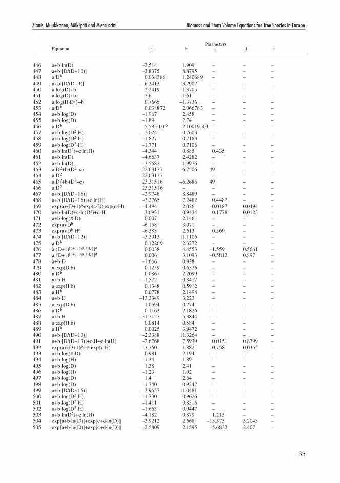
35
Zianis, Muukkonen, Mäkipää and Mencuccini Biomass and Stem Volume Equations for Tree Species in Europe
446 a+b·ln(D) –3.514 1.909 – – –447 a+b·[D/(D+10)] –3.8375 8.8795 – – –448 a·Db 0.038386 1.�40689 – – –449 a+b·[D/(D+9)] –6.3413 13.�90� – – –450 a·log(D)+b �.�419 –1.3705 – – –451 a·log(D)+b �.6 –1.61 – – –45� a·log(H·D�)+b 0.7665 –1.3736 – – –453 a·Db 0.03887� �.066783 – – –454 a+b·log(D) –1.967 �.458 – – –455 a+b·log(D) –1.89 �.74 – – –456 a·Db 5.595·10–5 �.10019503 – – –457 a+b·log(D�·H) –�.0�4 0.7603 – – –458 a+b·log(D�·H) –1.8�7 0.7183 – – –459 a+b·log(D�·H) –1.771 0.7106 – – –460 a+b·ln(D�)+c·ln(H) –4.344 0.885 0.435 – –461 a+b·ln(D) –4.6637 �.4�8� – – –46� a+b·ln(D) –3.568� 1.9976 – – –463 a·D�+b·(D�–c) ��.63177 –6.7506 49 – –464 a·D� ��.63177 – – – –465 a·D�+b·(D�–c) �3.31516 –6.�686 49 – –466 a·D� �3.31516 – – – –467 a+b·[D/(D+16)] –�.9748 8.8489 – – –468 a+b·[D/(D+16)]+c·ln(H) –3.�765 7.�48� 0.4487 – –469 exp(a)·(D+1)b·exp(c·D)·exp(d·H) –4.494 �.0�6 –0.0187 0.0494 –470 a+b·ln(D)+c·ln(D�)+d·H 3.6931 0.9434 0.1778 0.01�3 –471 a+b·log(π·D) 0.007 �.146 – – –47� exp(a)·Db –6.158 3.071 – – –473 exp(a)·Db·Hc –6.383 �.613 0.569 – –474 a+b·[D/(D+1�)] –3.3913 11.1106 – – –475 a·Db 0.1��69 �.3�7� – – –476 a·(D+1)[b+c·log(D)]·Hd 0.0038 4.4553 –1.5591 0.5661 –477 a·(D+1)[b+c·log(D)]·Hd 0.006 3.1093 –0.581� 0.897 –478 a+b·D –1.666 0.9�8 – – –479 a·exp(D·b) 0.1�59 0.65�6 – – –480 a·Db 0.0867 �.�099 – – –481 a+b·H –1.57� 0.8417 – – –48� a·exp(H·b) 0.1348 0.591� – – –483 a·Hb 0.0778 �.1498 – – –484 a+b·D –13.3349 3.��3 – – –485 a·exp(D·b) 1.0594 0.�74 – – –486 a·Db 0.1163 �.18�6 – – –487 a+b·H –31.71�7 5.3844 – – –488 a·exp(H·b) 0.0814 0.584 – – –489 a·Hb 0.00�5 3.947� – – –490 a+b·[D/(D+13)] –�.3388 11.3�64 – – –491 a+b·[D/(D+13)]+c·H+d·ln(H) –�.6768 7.5939 0.0151 0.8799 –49� exp(a)·(D+1)b·Hc·exp(d·H) –3.760 1.88� 0.758 0.0355 –493 a+b·log(π·D) 0.981 �.194 – – –494 a+b·log(H) –1.34 1.89 – – –495 a+b·log(D) 1.38 �.41 – – –496 a+b·log(H) –1.�3 1.9� – – –497 a+b·log(D) 1.4 �.64 – – –498 a+b·log(D) –1.740 0.9�47 – – –499 a+b·[D/(D+15)] –3.9657 11.0481 – – –500 a+b·log(D�·H) –1.730 0.96�6 – – –501 a+b·log(D�·H) –1.411 0.8316 – – –50� a+b·log(D�·H) –1.663 0.9447 – – –503 a+b·ln(D�)+c·ln(H) –4.18� 0.879 1.�15 – –504 exp[a+b·ln(D)]+exp[c+d·ln(D)] –3.9�1� �.668 –13.575 5.�043 –505 exp[a+b·ln(D)]+exp[c+d·ln(D)] –�.5809 �.1595 –5.683� �.407 –
Parameters Equation a b c d e

36
Silva Fennica Monographs 4 2005
506 Norway SW g cm – 7–15 – 6 7 16 0.99�507 Norway SW g cm – �–7 – 6 7 16 –508 Norway SW g cm – 7–�0 – 6 7 30 16 0.991509 Norway SW g cm – �–7 – 6 7 30 16 –510 Sweden ln(SW) kg cm – 0–45 0– 50 8 461 0.966511 Sweden ln(SW) kg cm m 0–45 0– 50 8 461 0.98651� Sweden ln(SW) g cm dm 1.1–10 1.7–8.8 19 8 84 0.98Pinus taeda513 – log(RT) kg cm – – – 68 8 7 0.863Populus tremula (European aspen, Asp)514 Germany AB kg cm – 13.�–33 15.9–�4.7 66 11 16 0.941515 Sweden AB kg mm – 1.9–9.� 3.6–15.8 36 4 – 0.958516 Sweden BR kg mm – 1.9–9.� 3.6–15.8 36 4 – 0.959517 Germany cR kg cm – 13.�–33 15.9–�4.7 66 11 16 0.9�5518 Sweden Fl kg mm – 1.9–9.� 3.6–15.8 36 4 – 0.944519 Germany ST kg cm – 13.�–33 15.9–�4.7 66 11 16 0.9095�0 Sweden ST kg mm – 1.9–9.� 3.6–15.8 36 4 – 0.95Populus trichocarpa (Black cottonwood)5�1 Iceland AB kg cm m 4.6–34 4.6–�0.7 71 8 �� 0.985�� Iceland cR kg cm m 4.6–34 4.6–�0.7 71 8 �� 0.8845�3 Iceland ST kg cm m 4.6–34 4.6–�0.7 71 8 �� 0.98Pseudotsuga menziesii (Douglas–fir) 5�4 Italy ln(AB) kg cm – 8.7–�7 – 5� 14 36 69 0.945�5 Netherlands AB kg cm – 3–38 6.7–�5.9 4 14 �3 0.9955�6 Netherlands AB kg cm – 5– – 30 9 – –5�7 Netherlands ln(ABW) kg cm – 5– – 30 9 – –5�8 Netherlands BR kg cm m 3–38 6.7–�5.9 4 14 �3 0.9445�9 Netherlands cR kg cm m 3–38 6.7–�5.9 4 14 �3 0.945530 UK cR kg cm m – – 9 6 � – –531 Netherlands Fl kg cm m 3–38 6.7–�5.9 4 14 �3 0.94153� – log(RT) kg cm – – – 68 8 18 0.908533 – log(RT) kg cm – – – 68 8 33 0.90�534 – log(RT) kg cm – – – 68 8 14 0.907535 – log(RT) kg cm – – – 68 8 3 0.966536 – log(RT) kg cm m – – 68 8 3 0.947537 UK RT t cm – – – 9 6 – –538 Netherlands ST kg cm m 3–38 6.7–�5.9 4 14 �3 0.998Pseudotsuga spp.539 Netherlands log(RT) kg cm – 5–�7 – �1 8 �1 0.96Quercus conferta (Hungarian oak, Platifilos dris)540 Greece ln(ABW) kg cm – �–19 �.�–14.7 51 14 �7 0.98541 Greece ln(ABW) kg cm cm �–19 �.�–14.7 51 14 �7 0.9854� Greece ln(BR) kg cm – �–19 �.�–14.7 51 14 37 �7 0.8�543 Greece BR kg cm – �–19 �.�–14.7 51 14 38 �7 0.65544 Greece ln(BR) kg cm – �–19 �.�–14.7 51 14 39 �7 0.73545 Greece ln(BR) kg cm – �–19 �.�–14.7 51 14 40 �7 0.89546 Greece ln(BR) kg cm cm �–19 �.�–14.7 51 14 37 �7 0.79547 Greece BR kg cm cm �–19 �.�–14.7 51 14 38 �7 0.5548 Greece ln(BR) kg cm cm �–19 �.�–14.7 51 14 39 �7 0.68549 Greece ln(BR) kg cm cm �–19 �.�–14.7 51 14 40 �7 0.86550 Greece ln(SW) kg cm – �–19 �.�–14.7 51 14 41 �7 0.96551 Greece ln(SW) kg cm – �–19 �.�–14.7 51 14 4� �7 0.8955� Greece ln(SW) kg cm – �–19 �.�–14.7 51 14 43 �7 0.97553 Greece ln(SW) kg cm cm �–19 �.�–14.7 51 14 41 �7 0.98554 Greece ln(SW) kg cm cm �–19 �.�–14.7 51 14 4� �7 0.89555 Greece ln(SW) kg cm cm �–19 �.�–14.7 51 14 43 �7 0.98Quercus ilex (Holm oak)556 Italy AB kg cm – �0–90 – 73 14 – –557 Italy AB kg cm – 5–�0 – 47 14 1� –558 Italy AB kg cm m 4.5–�6.1 6–16 7 8 94 0.95�
Appendix A Unit of Range of Biom. D H D (cm) H (m) Ref. cont. comm. n r�

37
Zianis, Muukkonen, Mäkipää and Mencuccini Biomass and Stem Volume Equations for Tree Species in Europe
506 a·D�+b·(D�–c) 89.�4474 64.89�5 49 – –507 a·D� 89.�4474 – – – –508 a·D�+b·(D�–c) 175.40886 1.7509 49 – –509 a·D� 175.40886 – – – –510 a+b·[D/(D+14)] –�.�184 11.4�19 – – –511 a+b·[D/(D+14)]+c·H+d·ln(H) –�.6864 7.6066 0.0�00 0.8658 –51� a+b·ln(D)+c·ln(D�)+d·H 4.38�3 1.19 0.1969 0.0149 –
513 a·log(D)+b 3.074� –�.6683 – – –
514 a·Db 0.0519 �.545 – – –515 a·Db 1.46·10–4 �.6035333 – – –516 a·Db 5.75·10–4 1.873�98 – – –517 a·Db 0.0644 �.001 – – –518 a·Db 8.47·10–4 1.481578 – – –519 a·Db 0.0197 �.764 – – –5�0 a·Db 6.5·10–5 �.7398�3 – – –
5�1 a·Db·Hc 0.0717 1.83�� 0.6397 – –5�� a·Db·Hc 0.0586 �.8�85 –1.0�8� – –5�3 a·Db·Hc 0.0379 1.581 1.0795 – –
5�4 a+b·ln(D) –1.957 �.�996 – – –5�5 a+b·ln(D) –1.6� �.410 – – –5�6 a·Db 0.111 �.397 – – –5�7 a·Db 0.111 �.397 – – –5�8 a+b·ln(D)+c·ln(H) –�.675 4.4�0 –�.784 – –5�9 a+b·ln(D)+c·ln(H) –1.345 3.9�4 –�.514 – –530 a·Db·Hc 3.461·10–4 �.7169 –1.�6060 – –531 a+b·ln(D)+c·ln(H) –1.346 3.351 –�.�01 – –53� a·log(D)+b �.1641 –1.4467 – – –533 a·log(D)+b �.5786 –1.8899 – – –534 a·log(D)+b �.9108 –�.3807 – – –535 a·log(D)+b �.5309 –1.6393 – – –536 a·log(H·D�)+b 1.047� –�.6�87 – – –537 a·Db �.179·10–5 �.4�09 – – –538 a+b·ln(D)+c·ln(H) –�.535 �.009 0.709 – –
539 a+b·log(D) –� �.63 – – –
540 a+b·ln(D) –�.1686 �.4407 – – –541 a+b·ln(D�H) –�.5�59 0.8605 – – –54� a+b·ln(D) –3.3508 1.7�35 – – –543 [a+b(1/D)+c(1/D�)]·D� 0.0536 –0.3�69 – – –544 a+b·ln(D) –11.433 4.9391 – – –545 a+b·ln(D) –4.1909 �.5403 – – –546 a+b·ln(D�H) –3.5363 0.5957 – – –547 [a+b(1/D�H)]·D�·H 0.0015 0.040� – – –548 a+b·ln(D�H) –1�.7333 1.8�0� – – –549 a+b·ln(D�H) –4.470� 0.8791 – – –550 a+b·ln(D) –�.5518 �.3887 – – –551 a+b·ln(D) –3.8649 �.4�61 – – –55� a+b·ln(D) –�.3� �.4147 – – –553 a+b·ln(D�H) –�.9�75 0.8468 – – –554 a+b·ln(D�H) –4.�1�� 0.854 – – –555 a+b·ln(D�H) –�.6916 0.8546 – – –
556 a·Db 0.�306 �.�791 – – –557 a·Db 0.�179 �.0513 – – –558 a+b·D�·H –0.6165 0.0358� – – –
Parameters Equation a b c d e

38
Silva Fennica Monographs 4 2005
559 Spain log(AB) kg cm – 5.3–�4.4 4.4–1�.8 1� 8 69 0.908560 Spain log(AB) kg cm – 5.3–�4.4 4.4–1�.8 1� 8 33 0.91561 Spain log(AB) kg cm – 5.3–�4.4 4.4–1�.8 1� 8 30 0.9�756� Spain log(AB) kg cm – 5.3–�4.4 4.4–1�.8 1� 8 41 0.939563 Spain log(AB) kg cm – 5.3–�4.4 4.4–1�.8 1� 8 �8 0.867564 Spain log(AB) kg cm m 5.3–�4.4 4.4–1�.8 1� 8 63 0.94�565 Spain AB kg cm – – – �5 14 15 –566 Italy ABW kg cm m 4.5–�6.1 6–16 7 8 3 94 0.95�567 Spain log(BR) kg cm – 5.3–�4.4 4.4–1�.8 1� 8 44 69 0.803568 Spain log(BR) kg cm – 5.3–�4.4 4.4–1�.8 1� 8 44 33 0.784569 Spain log(BR) kg cm – 5.3–�4.4 4.4–1�.8 1� 8 44 30 0.697570 Spain log(BR) kg cm – 5.3–�4.4 4.4–1�.8 1� 8 44 41 0.84571 Spain log(BR) kg cm – 5.3–�4.4 4.4–1�.8 1� 8 44 �8 0.77557� Spain log(BR) kg cm m 5.3–�4.4 4.4–1�.8 1� 8 44 63 0.807573 Spain log(BR) kg cm – 5.3–�4.4 4.4–1�.8 1� 8 45 56 0.781574 Spain log(BR) kg cm – 5.3–�4.4 4.4–1�.8 1� 8 46 69 0.443575 Italy cR kg cm m 4.5–�6.1 6–16 7 8 94 0.95�576 Spain log(Fl) kg cm – 5.3–�4.4 4.4–1�.8 1� 8 69 0.615577 Spain log(Fl) kg cm – 5.3–�4.4 4.4–1�.8 1� 8 33 0.467578 Spain log(Fl) kg cm – 5.3–�4.4 4.4–1�.8 1� 8 30 0.65579 Spain log(Fl) kg cm – 5.3–�4.4 4.4–1�.8 1� 8 41 0.735580 Spain log(Fl) kg cm – 5.3–�4.4 4.4–1�.8 1� 8 �8 0.74581 Spain log(Fl) kg cm m 5.3–�4.4 4.4–1�.8 1� 8 63 0.59358� Spain log(Rc) kg cm – 7.�–�3.1 4.4–1�.8 13 8 �5 31 0.64583 Spain log(Rc) kg cm – 7.�–�3.1 4.4–1�.8 13 8 �5 19 0.7584 Spain log(Rc) kg cm – 8.8–19.8 5.5–9.0 13 8 �5 1� 0.7585 Spain log(RS) kg cm – 7.�–�3.1 4.4–1�.8 13 8 47 31 0.67586 Spain log(RS) kg cm – 7.�–�3.1 4.4–1�.8 13 8 47 19 0.75587 Spain log(RS) kg cm – 8.8–19.8 5.5–9.0 13 8 47 1� 0.63588 Spain log(RT) kg cm – 7–�3 – �1 8 3� 0.73589 Spain log(RT) kg cm – 7.�–�3.1 4.4–1�.8 13 8 3� 0.73590 Spain log(RT) kg cm – 7.�–�3.1 4.4–1�.8 13 8 �0 0.81591 Spain log(RT) kg cm – 8.8–19.8 5.5–9.0 13 8 1� 0.7159� Spain log(ST) kg cm – 5.3–�4.4 4.4–1�.8 1� 8 � 71 0.918593 Spain log(ST) kg cm – 5.3–�4.4 4.4–1�.8 1� 8 � 33 0.9�9594 Spain log(ST) kg cm – 5.3–�4.4 4.4–1�.8 1� 8 � 3� 0.958595 Spain log(ST) kg cm – 5.3–�4.4 4.4–1�.8 1� 8 � 43 0.941596 Spain log(ST) kg cm – 5.3–�4.4 4.4–1�.8 1� 8 � �8 0.88�597 Spain log(ST) kg cm m 5.3–�4.4 4.4–1�.8 1� 8 � 65 0.963Quercus petraea598 France log(RT) kg cm – 7–17 – �1 8 71 0.94Quercus pyrenaica (Pyrenean oak)599 Portugal ln(SW) kg cm m �.5–46 3.3–�7 14 8 166 0.99Quercus spp. (Oak, Eiche)600 Austria ln(AB) kg cm – – – 31 3 33 –601 UK ln(ABW) kg cm – 4.5–5� – 10 14 11 �0 0.9960� UK ln(ABW) kg cm – 4.3–35 – 10 14 11 16 0.99603 UK ln(ABW) kg cm – 3.8–11 – 10 14 11 15 0.974604 UK ln(ABW) kg cm – 5.7–33 – 10 14 11 18 0.995605 UK cR t cm – – – 9 6 1 – –606 UK cR t cm m – – 9 6 � – –Tilia cordata (lime)607 UK ln(ABW) kg cm – 3.�–15 – 10 14 11 10 0.984
Appendix A Unit of Range of Biom. D H D (cm) H (m) Ref. cont. comm. n r�

39
Zianis, Muukkonen, Mäkipää and Mencuccini Biomass and Stem Volume Equations for Tree Species in Europe
559 a+b·log(D) –0.656 �.�17 – – –560 a+b·log(D) –0.�75 1.831 – – –561 a+b·log(D) –0.854 �.413 – – –56� a+b·log(D) –0.90� �.433 – – –563 a+b·log(D) –0.313 1.900 – – –564 a+b·log(D)+c·H –0.568 1.953 0.0�9 – –565 a·Db 0.�313 �.�66� – – –566 a+b·D�·H –1.0906 0.031073 – – –567 a+b·log(D) –0.704 1.833 – – –568 a+b·log(D) –0.411 1.546 – – –569 a+b·log(D) –0.8�5 1.953 – – –570 a+b·log(D) –0.996 �.077 – – –571 a+b·log(D) –0.370 1.544 – – –57� a+b·log(D)+c·H –0.617 1.67� 0.014 – –573 a+b·log(D) –0.8�5 1.789 – – –574 a+b·log(D) –1.4�9 �.089 – – –575 a+b·D�·H 0.4741 0.0047473 – – –576 a+b·log(D) –1.6�4 1.891 – – –577 a+b·log(D) –1.347 1.654 – – –578 a+b·log(D) –�.1�8 �.309 – – –579 a+b·log(D) –�.14� �.�69 – – –580 a+b·log(D) –1.366 1.774 – – –581 a+b·log(D)+c·H –1.533 1.808 0.00� – –58� a+b·log(D) –1.188 �.139 – – –583 a+b·log(D) –1.563 �.4�� – – –584 a+b·log(D) –0.714 1.79 – – –585 a+b·log(D) –1.145 1.897 – – –586 a+b·log(D) –1.417 �.093 – – –587 a+b·log(D) –0.835 1.688 – – –588 a+b·log(D) –1.05 �.19 – – –589 a+b·log(D) –1.047 �.191 – – –590 a+b·log(D) –1.393 �.451 – – –591 a+b·log(D) –0.448 1.734 – – –59� a+b·log(D) –1.166 �.478 – – –593 a+b·log(D) –0.747 �.044 – – –594 a+b·log(D) –1.355 �.674 – – –595 a+b·log(D) –1.336 �.640 – – –596 a+b·log(D) –0.839 �.156 – – –597 a+b·log(D)+c·H –1.088 �.157 0.039 – –
598 a+b·log(D) –1.56 �.44 – – –
599 a+b·ln(H·D�) –3.3�3 0.95 – – –
600 a+b·ln(D) –0.883 �.140 – – –601 a+b·ln(D) –�.4�3� �.468� – – –60� a+b·ln(D) –�.3��3 �.40�9 – – –603 a+b·ln(D) –3.1404 �.8113 – – –604 a+b·ln(D) –3.1009 �.6996 – – –605 a·D� �.161�·10–4 – – –606 a·Db·Hc 5.4��4·10–4 �.35 –1.0�� – –
607 a+b·ln(D) –�.6788 �.454� – – –
Parameters Equation a b c d e

40
Silva Fennica Monographs 4 2005
References – Appendix A
1 Albrektson, A., Valinger, E. & Jonson, c. 1984. Några funktioner för bestämning av tallars biomassa i södra Norrland. Sveriges Skogsvårdsförbunds Tidskrift 8�(6): 5–1�.
� Baldini, S., Berti, S., cutini, A., Mannucci, M., Mer-curio, R. & Spinelli, R. 1989. Prove sperimentali di primo diradamento in un soprassuolo di pino marittimo (Pinus pinaster Ait.) originato da incendio: aspetti silvicolturali, di utilizzazione e caratteristiche della biomassa. Ann. Ist. Sper. Selvicoltura �0: 385–436.
3 Barcikowski, A. & loro, P.M. 1995. Needle biomass and dendrometrical features of Scots pine (Pinus syl-vestris l.) natural regeneration seedlings of younger age classes, qrowing on a fresh coniferous forest site. Sylwan 139(�): 53–6�.
4 Bartelink, H.H. 1996. Allometric relationships on bio-mass and needle area of Douglas-fir. Forest Ecology and Management 86: 193–�03.
5 Bartelink, H.H. 1997. Allometric relationship for bio-mass and leaf area of beech (Fagus sylvatica l). Annals of Forest Science 54: 39–50.
6 Brække, F.H. 1986. Distribution and yield of biomass from young Pinus sylvestris and Picea abies stands on draines and fertilized peatland. Scandinavian Journal of Forest Research 1: 49–66.
7 Brandini, P. & Tabacchi, G. 1996. Biomass and volume equations for holm oak and straberry-tree in coppice stands of Southern Sardinia. ISAFA communicazioni di Ricerca 96(1): 59–69.
8 Briggs, E.F. & cunia, T. 198�. Effect of cluster sam-pling in biomass tables construction: linear regression models. canadian Journal of Forest Research 1�(�): �55–�63.
9 Broadmeadow, M. & Matthews, R. �004. Survey meth-ods for Kyoto Protocol monitoring and verification of UK forest carbon stocks. UK Emissions by Sources and Removals by Sinks due to land Use, land Use change and Forestry Activities, Report. cEH, Edinburgh (June �004).
10 Bunce, R.G.H. 1968. Biomass and production of trees in a mixed deciduoud woodland. I. Girth and height as parameters for the estimation of tree dry weight. Journal of Ecology 56: 759–775.
11 calamini, G. & Gregori, E. �001. Study in a beech stand of central Italy: allometric relations for the above ground biomass estimation. l’Italia Forestale e Montana 56(1): 1–�3.
1� canadell, J., Riba, M. & Andrés, P. 1988. Biomass equations for Quercus ilex l. in the Montseny Massif, Northeastern Spain. Forestry 61(�): 137–147.
13 canadell, J. & Rodà, F. 1991. Root biomass of Quer-cus ilex in a montane mediterranean forest. canadian Journal of Forest Research �1: 1771–1778.
14 carvalho, J.P. & Parresol, B.R. �003. Additivity in tree biomass components of Pyrenean oak (Quercus
pyrenaica Willd.). Forest Ecology and Management 179: �69–�76.
15 cienciala, E., cerný, M., Alptauer, J. & Exnerová, Z. �005. Biomass functions applicable to European beech. Journal of Forest Science 51(4): 147–154.
16 cerný, M. 1990. Biomass of Picea abies (l.) Karst. in midwestern Bohemia. Scandinavian Journal of Forest Research 5: 83–95.
17 chroust, l. 1985. Above-ground biomass of young pine forests (Pinus sylvestris) and its determination. communicationes Instituti Forestalis cechosloveniae 14: 1�7–145.
18 chroust, l. & Tesarova, J. 1985. Quatification of above-ground components of �0 years old Norway spruce (Picea abies (l.) Karsten). communicationes Instituti Forestalis cechosloveniae 14: 111–1�6.
19 claesson, S., Sahlén, K. & lundmark, T. �001. Func-tions for biomass estimation of young Pinus sylvestris, Picea abies and Betula spp. from stands in northern Sweden with high stand densities. Scandinavian Jour-nal of Forest Research 16: 138–146.
�0 Dietrich, H.-P., Raspe, S., Schwarzmeier, M. & Ilg, S. �00�. Biomasse- und Nährelementinventuren zur Ermittlung von Ernteentzügen an drei bayerischen Fichtenstandorten. In: Dietrich, H.-P., Raspe, S. & Preuhsler, T. (eds.): Inventur von Biomasse- und Nährstoffvorräten in Waldbeständen. Forstliche For-schungsberichte, München, 186: 59–7�.
�1 Drexhage, M. & colin, F. �001. Estimating root system biomass from breast-height diameters. Forestry 74(5): 491–497.
�� Drexhage, M. & Gruber, F. 1999. Above- and below-stump relationships for Picea abies: Estimating root system biomass from breast-height diameters. Scan-dinavian Journal of Forest Research 14: 3�8–333.
�3 Duvigneaud, P., Kestemont, P., Timperman, J. & Moni-quet, J.-c. 1977. la hetraie ardennaise a Festuca Alt-issima a mirwart biomasse et productivite primaire. In: Duvigneaud, P. & Kestemont, P. (eds.). Productivite biologique en Belgique. Editions Duculot, Paris-Gem-bloux. p. 107–154.
�4 Duvigneaud, P. & Timperman, P. 1977. Biomasse des epiphytes cryptogamiques dans une hêtraie ardennaise. In: Duvigneaud, P. & Kestemont, P. (eds.). Productivite biologique en Belgique. Editions Duculot, Paris-Gem-bloux.
�5 Ferres, l., Roda, F., Verdu, A.M.c. & Terradas, J. 1980. Estructura y funcionalismo de un encinar montano en el Montseny. II. Biomasa aera. Mediterranea 4: �3–36.
�6 Fiedler, F. 1986. Die Dendromasse eines hiebsreifen Fichtenbestandes. Beiträge für die Forstwirtschaft �0(4): 171–180.
�7 Fiedler, F. 1987. Das Ökologische Meßfeld der Sek-tion Forstwirtschaft der TU Dresden. V. Die Verteilung der Dendromassekomponenten. Wissenschaftliche Zeitschrift der Technischen Universität Dresden 36(6): ��9–�34.

41
Zianis, Muukkonen, Mäkipää and Mencuccini Biomass and Stem Volume Equations for Tree Species in Europe
�8 Hakkila, P. 1971. coniferous branches as a raw material source. communicationes Instituti Forestalis Fenniae 75(1): 1–60.
�9 Hakkila, P. 1991. Hakkuupoistuman latvusmassa. Folia Forestalia 773: 1–�4.
30 Hees, A.F.M.v. �001. Biomass development in unman-aged forests. Nederlands Bosbouwtijdschrift 73(5): �–5.
31 Hochbichler, E. �00�. Vorläufige Ergebnisse von Biomasseninventuren in Buchen- und Mittelwald-beständen. In: Dietrich, H.-P., Raspe, S. & Preuhsler, T. (eds.): Inventur von Biomasse- und Nährstoffvor-räten in Waldbeständen. Forstliche Forschungsberichte, München, 186: 37–46
3� Hughes, M.K. 1971. Tree biocontent, net production and litter fall in a deciduous woodland. Oikos ��: 6�–73.
33 Ilg, S. �00�. Erhebung der oberirdischen Biomasse- und Elementvorräte eines Fichtenbestandes (Picea abies (l.) Karst.) im Bereich der Waldklimastation Zusmarshausen. Fachhochschule Weihenstephan. Fachbereich Forstwirtschaft. 98 p.
34 Ingerslev, M. & Hallbäcken, l. 1999. Above ground biomass and nutrient distribution in a limed and ferti-lized Norway spruce (Picea abies) plantation. Part II. Accumulation of biomass and nutrients. Forest Ecology and Management 119: �1–38.
35 Johansson, T. 1999a. Biomass equations for deter-mining functions of pendula and pubescent birches growing on abandoned farmland and some practical implicatons. Biomass and Bioenergy 16: ��3–�38.
36 Johansson, T. 1999b. Biomass equations for determin-ing functions of European aspen growing on abandoned farmland and some practical implicatons. Biomass and Bioenergy 17: 471–480.
37 Johansson, T. 1999c. Biomass production of Norway spruce (Picea abies (l.) Karst.) growing on abandoned farmland. Silva Fennica 33(4): �61–�80.
38 Johansson, T. 1999d. Dry matter amounts and incre-ment in �1- to 91-year-old common alder and grey alder and some practical implications. canadian Journal of Forest Research �9: 1679–1690.
39 Johansson, T. �000. Biomass equations for determin-ing functions of common and grey alder growing on abandoned farmland and some practical implicatons. Biomass and Bioenergy 18: 147–159.
40 Korhonen, K.T. & Maltamo, M. 1990. Männyn maan-päällisten osien kuivamassat Etelä-Suomessa. Metsän-tutkimuslaitoksen tiedonantoja 371: 1–�9.
41 laitat, E., lebègue, c., Perrin, D. & Pissart, G. �003. Séquestration du carbone par les forêts selon l’affectation des terres. Ministre de l’Agriculture et de la Ruralité, Ministère de la Région Wallonne, Division de la Nature et des Forêts, FuSAGxp.
4� le Goff, N. & Ottorini, J.M. �000. Biomass distributions at tree and stand levels in the beech experimental forest of Hesse (NE France). Viterbo (November): 9–11.
43 le Goff, N. & Ottorini, J.M. �001. Root biomass and biomass increment in a beech (Fagus sylvatica l.) stand in North-East France. Annals of Forest Science 58: 1–13.
44 lee, D.-H. 1998. Architektur des Wurzelsystems von Fichten (Picea abies [l.] Karst.) auf unterschiedlich versauerten Standorten. Göttingen, Forschungszentrum Waldökosysteme der Universität Göttingen. Reihe A 153: 1–14�.
45 lee, D.-H. �001. Relationship between above- and below-ground biomass for Norway spruce (Picea abies): estimating root system biomass from breast height diameter. Jour. Korean For. Soc. 90(3): 338–345.
46 lehtonen, A. �005. Estimating foliage biomass for Scots pine (Pinus sylvestris l.) and Norway spruce (Picea abies (l.) Karst.) plots. Tree Physiology �5: 803–811.
47 leonardi, S. & Rapp, M. 198�. Phytomasse et miner-alomase d’un taillis de chene Vert du Massif de l’Etna. Ecologia Mediterranea 8: 1�5–138.
48 lim, M.T. & J.E., c. 1986. The internal transfer of nutrients in a Scots pine stand: biomass components, current growth and their nutrient content. Forestry 59(1): 1–�7.
49 Marklund, l.G. 1987. Biomass functions for Norway spruce (Picea abies (l.) Karst.) in Sweden. Sveriges lantbruksuniversitet, Institutionen för skogstaxering, Rapport 43: 1–1�7.
50 Marklund, l.G. 1988. Biomassafunktioner för tall, gran och björk i Sverige. Sveriges lantbruksuniversitet, Institutionen för skogstaxering, Rapport 45: 1–73.
51 Matis, K. & Alifragis, D. 1983–1984. Aboveground biomass of oaks (Quercus conferta Kit.) in Taxiarchis Greece. Scientific Annals of the Depart. of Forestry and Natural Envir. KA 15.
5� Menguzzato, G. & Tabacchi, G. 1986. Prove di dirada-mento su Pseudotsuga menziesii in calabria. Ambiente, tavole di cubatura e della biomassa epigea. Ann. Ist. Sper. Selvicoltura 17: �55–�93.
53 Menguzzato, G. 1988. Modelli di previsione del peso fresco, della biomassa e del volume per pino insigne ed eucalitti nell’Azienda Massanova (Salerno). Ann. Ist. Sper. Selvicoltura 19: 3�3–354.
54 Mund, M., Kummetz, E., Hein, M., Bauer, G.A. & Schulze, E.-D. �00�. Growth and carbon stocks of a spruce forest chronosequence in central Europe. Forest Ecology and Management 171: �75–�96.
55 Mäkelä, A. & Vanninen, P. 1998. Impacts of size and competition on tree form and distribution of above-ground biomass in Scots pine. canadian Journal of Forest Research �8: �16–��7.
56 Mälkönen, E. 1974. Annual primary production and nutrient cycle in some Scots pine stands. communi-cationes Instituti Forestalis Fenniae 84(5): 1–87.
57 Mälkönen, E. 1977. Annual primary production and nutrient cycle in birch stand. communicationes Instituti Forestalis Fenniae 91(5): 1–35.

4�
Silva Fennica Monographs 4 2005
58 Mälkönen, E. & Saarsalmi, A. 198�. Hieskoivikon biomassatuotos ja ravinteiden menetys kokopuun kor-juussa. Folia Forestalia 534: 1–17.
59 Møller, I.S. �000. calculation of biomass and nutri-ent removal for different harvesting intensities. New Zealand Journal of Forestry Science 30(1): �9–45.
60 Neumann, M. & Jandl, R. �00�. Aboveground biomass of two young Norway spruce stands. Manuscript.
61 Nihlgård, B. 197�. Plant biomass, primary production and distribution of chemical elements in a beech and a planted spruce forest in South Sweden. Oikos �3: 69–81.
6� Oleksyn, J., Reich, P.B., chalupka, W. & Tjoelker, M.G. 1999. Differential above- and below-ground biomass accumulation of European Pinus sylvestris populations in a 1�-year-old provenance experiment. Scandinavian Journal of Forest Research 14: 7–17.
63 Ovington, J.D. 1957. Dry matter production by Pinus sylvestris l. Annals of Botany �1(8�): �87–314.
64 Poeppel, B. 1989. Untersuchungen der Dendromasse in mittelalten Fichtenbeständen. Forsteinrichtung und Forstliche Ertragskunde, Technische Universität Dres-den. 66 p.
65 Pretzsch, H. �000. Die Regeln von Reineke, Yoda und das Gesetz der räumlichen Allometrie. Allgemeine Forst- und Jagd-Zeitung 171: �05–�10.
66 Rock, J. �005. Suitability of published equations for aspen in central Europe – results from a case study. Submitted manuscript.
67 Santa Regina, I. & Tarazona, T. �001. Organic matter and nitrogen dynamics in a mature forest of common beech in the Sierra de la Demanda, Spain. Ann. Sci. For. 58: 301–314.
68 Santantonio, D., Hermann, R.K. & Overton, W.S. 1977. Root biomass studies in forest ecosystems. Pedobio-logia 17: 1–31.
69 Schwarzmeier, M. �000. Erhebung der oberirdischen Biomassevorräte von Fichtenbeständen (Picea abies (l.) Karst.) im Bereich der Waldklimastationen Eber-sberg und Flossenbürg. Diploma Thesis, Fachhoch-schule Weihenstephan, Fachbereich Forstwirtschaft, Germany 155 p.
70 Schöpfer, W. 1961. Beiträge zur Erfassung des Assimi-lationsapparates der Fichte. 1�7 p.
71 Snorrason, A. & Einarsson, S.F. �004. Single-tree bio-mass and stem volume functions for eleven tree species used in Icelandic forestry. Submitted manuscript.
7� Starr, M., Hartman, M. & Kinnunen, T. 1998. Biomass functions for mountain birch in the Vuoskojärvi Inte-grated Monitoring area. Boreal Environment Research 3: �97–303.
73 Susmel, l., Viola, F. & Bassalo, G. 1976. Ecologie della lecceta del Supramonte di Orgosolo. (Sardegna centro-orientale). Analisi de centro di Economia Mon-tana delle Venezie 10: 1–�16.
74 Wirth, c., Schumacher, J. & Schulze, E.-D. �004. Generic biomass functions for Norway spruce in cen-
tral Europe – a meta-analysis approach toward predic-tion and uncertainty estimation. Tree Physiology �4: 1�1–139.
75 Xiao, c.W., curiel Yuste, J., Janssens, I.A., Roskams, P., Nachtergale, l., carrara, A., Sanchez, B.Y. & ceu-lemans, R. �003. Above-and belowground biomass and net primary production in a 73-year-old Scots pine forest. Tree Physiology �3: 505–516.
76 Zianis, D. & Mencuccini, M. �003. Aboveground bio-mass relationship for beech (Fagus moesiaca cz.) trees in Vermio Mountain, Northern Greece, and generalised equations for Fagus sp. Annals of Forest Science 60: 439–448.
77 The equation is derived from 3 different sources: Makkonen, K. & Helmisaari, H.-S. 1998. Seasonal and
yearly variations of fine-root biomass and necromass in a Scots pine (Pinus sylvestris l.) stand. Forest Ecology and Management 10�: �83–�90.
Oleksyn, J., Reich, P.B., chalupka, W. & Tjoelker, M.G. 1999. Differential above- and below-ground biomass accumulation of European Pinus sylvestris populations in a 1�-year-old provenance experiment. Scandinavian Journal of Forest Research 14: 7–17.
Vanninen, P., Ylitalo, H., Sievänen, R. & Mäkelä, A. 1996. Effects of age and site quality on the distribution of biomass in Scots pine (Pinus sylvestris l.). Trees 10: �31–�38.
Contact persons – Appendix A
1 Boosten M., [email protected], Wageningen University, the Netherlands
� Cienciala E., [email protected], Institute of Forest Ecosystem Research (IFER), czech Repub-lic
3 Hochbichler E., [email protected], Uni-versität für Bodenkultur, Wien
4 Johansson T., [email protected], SlU, Sweden
5 Laitat E., Department of Plant Biology, Gembloux Agricultural university
6 Matthews, R., [email protected], Forest Research, Alice Holt Research Station, UK
7 Møller I.S., [email protected], Danish centre for Forest, landscape and Planning
8 Muukkonen P., [email protected], Finnish Forest Research Institute, Finland
9 Nabuurs G.-J., [email protected], Alterra, Wageningen, the Netherlands
10 Raspe S., [email protected], Bayerische landesanstalt für Wald und Forstwirtschaft, Freis-ing, Germany

43
Zianis, Muukkonen, Mäkipää and Mencuccini Biomass and Stem Volume Equations for Tree Species in Europe
11 Rock, J., [email protected], Global change and Natural Systems Department, Potsdam Insti-tute for climate change Impact Research
1� Wirth C., [email protected], Max-Planck-Insitute for Biogeochemistry, Jena, Germany
13 Xiao C.W., [email protected], University of Ant-werpen, Belgium
14 Zianis D., TEI Kavalas, Greece
Comments – Appendix A
1 Trees 7 cm or less in diameter� Trees more than 7 cm in diameter3 Merchantable parts, >3–4 cm4 living branches5 Roots more than 1 cm in diameter6 Regressions developed by D Zianis. Original data
from tables7 0.3 m from forest floor8 Young trees9 Middle age trees10 Adult trees11 Original regressions relate girth to biomass1� D at tree base13 Other types of functions with D and H and inde-
pendent variables are given for the same material, includes determination coefficients
14 Newly cut trees15 cut trees dried in the stand during summer with
a total loss of needles of about 75%16 Includes fertilized plots17 Wood of all living branches18 Branch and top wood19 Wood and bark of all living branches�0 Twigs�1 living crown�� Whole crown�3 Other than current year needles, includes fertilized
plots�4 Includes needles, twigs, and branches less than
1 cm in diameter�5 Roots more than 5 cm in diameter�6 Roots less than 5 cm in diameter�8 Dominant trees over an age gradient�9 Trees of different sizes in one age group30 Fertilised plot
31 Doubt about the parameters.3� Doubt about the sign of the parameter c. The sign of
the parameter c has been changed on this table.33 One year old needles34 Two years old needles35 The equation is derived from 3 different sources: Makkonen, K. & Helmisaari, H.-S. 1998. Seasonal
and yearly variations of fine-root biomass and nec-romass in a Scots pine (Pinus sylvestris l.) stand. Forest Ecology and Management 10�: �83–�90.
Oleksyn, J., Reich, P.B., chalupka, W. & Tjoelker, M.G. 1999. Differential above- and below-ground biomass accumulation of European Pinus sylvestris populations in a 1�-year-old provenance experi-ment. Scandinavian Journal of Forest Research 14: 7–17.
Vanninen, P., Ylitalo, H., Sievänen, R. & Mäkelä, A. 1996. Effects of age and site quality on the dis-tribution of biomass in Scots pine (Pinus sylvestris l.). Trees 10: �31–�38.
The equation is based on 38 different values of total root biomass and diameter at breast height; some values were derived from individual trees; some values were averages from several trees.
36 Regressions developed by D Zianis. Original data from graphs
37 Branches less than or equal to 1 cm38 Branches between 1 and 3 cm39 Branches bigger than 3 cm40 All branches41 Stem wood beneath crown4� Stem wood in crown43 Total stem wood44 Branches less than 5 cm in diameter45 Branches 1 to 5 cm in diameter46 Branches greater than 5 cm in diameter
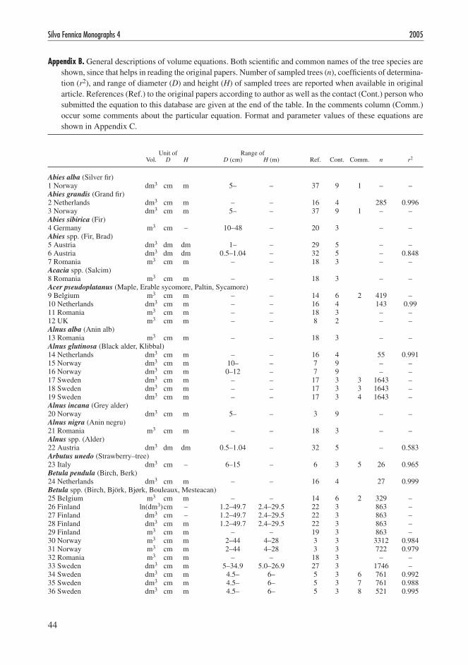
44
Silva Fennica Monographs 4 2005
Appendix B. General descriptions of volume equations. Both scientific and common names of the tree species are shown, since that helps in reading the original papers. Number of sampled trees (n), coefficients of determina-tion (r�), and range of diameter (D) and height (H) of sampled trees are reported when available in original article. References (Ref.) to the original papers according to author as well as the contact (cont.) person who submitted the equation to this database are given at the end of the table. In the comments column (comm.) occur some comments about the particular equation. Format and parameter values of these equations are shown in Appendix c.
Unit of Range of Vol. D H D (cm) H (m) Ref. cont. comm. n r�
Abies alba (Silver fir)1 Norway dm3 cm m 5– – 37 9 1 – –Abies grandis (Grand fir)� Netherlands dm3 cm m – – 16 4 �85 0.9963 Norway dm3 cm m 5– – 37 9 1 – –Abies sibirica (Fir)4 Germany m3 cm – 10–48 – �0 3 – –Abies spp. (Fir, Brad)5 Austria dm3 dm dm 1– – �9 5 – –6 Austria dm3 dm dm 0.5–1.04 – 3� 5 – 0.8487 Romania m3 cm m – – 18 3 – –Acacia spp. (Salcim)8 Romania m3 cm m – – 18 3 – –Acer pseudoplatanus (Maple, Erable sycomore, Paltin, Sycamore)9 Belgium m3 cm m – – 14 6 � 419 –10 Netherlands dm3 cm m – – 16 4 143 0.9911 Romania m3 cm m – – 18 3 – –1� UK m3 cm m – – 8 � – –Alnus alba (Anin alb)13 Romania m3 cm m – – 18 3 – –Alnus glutinosa (Black alder, Klibbal)14 Netherlands dm3 cm m – – 16 4 55 0.99115 Norway dm3 cm m 10– – 7 9 – –16 Norway dm3 cm m 0–1� – 7 9 – –17 Sweden dm3 cm m – – 17 3 3 1643 –18 Sweden dm3 cm m – – 17 3 3 1643 –19 Sweden dm3 cm m – – 17 3 4 1643 –Alnus incana (Grey alder)�0 Norway dm3 cm m 5– – 3 9 – –Alnus nigra (Anin negru)�1 Romania m3 cm m – – 18 3 – –Alnus spp. (Alder)�� Austria dm3 dm dm 0.5–1.04 – 3� 5 – 0.583Arbutus unedo (Strawberry–tree)�3 Italy dm3 cm – 6–15 – 6 3 5 �6 0.965Betula pendula (Birch, Berk)�4 Netherlands dm3 cm m – – 16 4 �7 0.999Betula spp. (Birch, Björk, Bjørk, Bouleaux, Mesteacan)�5 Belgium m3 cm m – – 14 6 � 3�9 –�6 Finland ln(dm3) cm – 1.�–49.7 �.4–�9.5 �� 3 863 –�7 Finland dm3 cm – 1.�–49.7 �.4–�9.5 �� 3 863 –�8 Finland dm3 cm m 1.�–49.7 �.4–�9.5 �� 3 863 –�9 Finland m3 cm m – – 19 3 863 –30 Norway m3 cm m �–44 4–�8 3 3 331� 0.98431 Norway m3 cm m �–44 4–�8 3 3 7�� 0.9793� Romania m3 cm m – – 18 3 – –33 Sweden dm3 cm m 5–34.9 5.0–�6.9 �7 3 1746 –34 Sweden dm3 cm m 4.5– 6– 5 3 6 761 0.99�35 Sweden dm3 cm m 4.5– 6– 5 3 7 761 0.98836 Sweden dm3 cm m 4.5– 6– 5 3 8 5�1 0.995
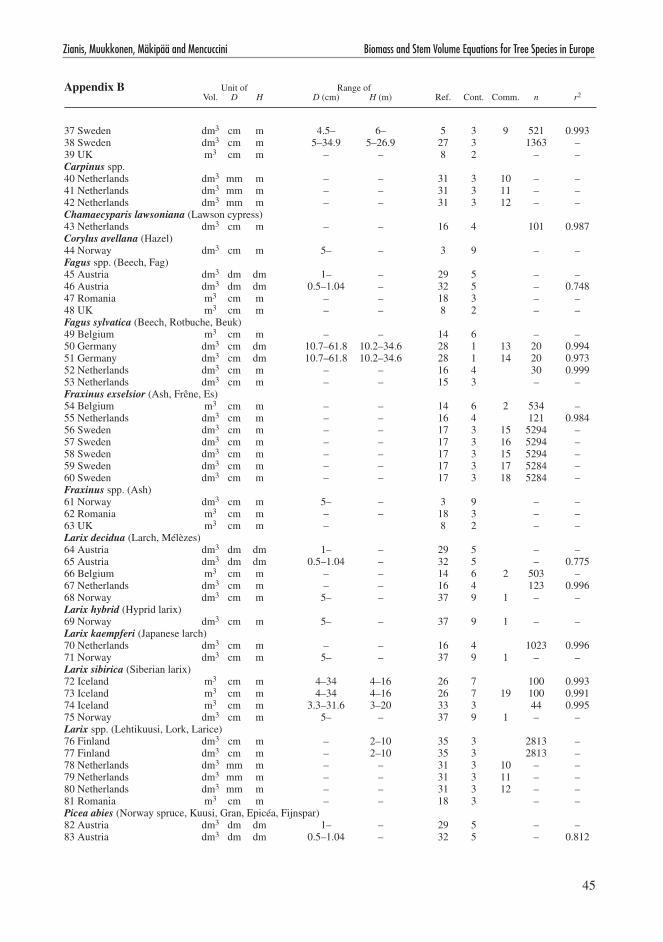
45
Zianis, Muukkonen, Mäkipää and Mencuccini Biomass and Stem Volume Equations for Tree Species in Europe
37 Sweden dm3 cm m 4.5– 6– 5 3 9 5�1 0.99338 Sweden dm3 cm m 5–34.9 5–�6.9 �7 3 1363 –39 UK m3 cm m – – 8 � – –Carpinus spp.40 Netherlands dm3 mm m – – 31 3 10 – –41 Netherlands dm3 mm m – – 31 3 11 – –4� Netherlands dm3 mm m – – 31 3 1� – –Chamaecyparis lawsoniana (lawson cypress)43 Netherlands dm3 cm m – – 16 4 101 0.987Corylus avellana (Hazel)44 Norway dm3 cm m 5– – 3 9 – –Fagus spp. (Beech, Fag)45 Austria dm3 dm dm 1– – �9 5 – –46 Austria dm3 dm dm 0.5–1.04 – 3� 5 – 0.74847 Romania m3 cm m – – 18 3 – –48 UK m3 cm m – – 8 � – –Fagus sylvatica (Beech, Rotbuche, Beuk)49 Belgium m3 cm m – – 14 6 – –50 Germany dm3 cm dm 10.7–61.8 10.�–34.6 �8 1 13 �0 0.99451 Germany dm3 cm dm 10.7–61.8 10.�–34.6 �8 1 14 �0 0.9735� Netherlands dm3 cm m – – 16 4 30 0.99953 Netherlands dm3 cm m – – 15 3 – –Fraxinus exselsior (Ash, Frêne, Es)54 Belgium m3 cm m – – 14 6 � 534 –55 Netherlands dm3 cm m – – 16 4 1�1 0.98456 Sweden dm3 cm m – – 17 3 15 5�94 –57 Sweden dm3 cm m – – 17 3 16 5�94 –58 Sweden dm3 cm m – – 17 3 15 5�94 –59 Sweden dm3 cm m – – 17 3 17 5�84 –60 Sweden dm3 cm m – – 17 3 18 5�84 –Fraxinus spp. (Ash)61 Norway dm3 cm m 5– – 3 9 – –6� Romania m3 cm m – – 18 3 – –63 UK m3 cm m – 8 � – –Larix decidua (larch, Mélèzes)64 Austria dm3 dm dm 1– – �9 5 – –65 Austria dm3 dm dm 0.5–1.04 – 3� 5 – 0.77566 Belgium m3 cm m – – 14 6 � 503 –67 Netherlands dm3 cm m – – 16 4 1�3 0.99668 Norway dm3 cm m 5– – 37 9 1 – –Larix hybrid (Hyprid larix)69 Norway dm3 cm m 5– – 37 9 1 – –Larix kaempferi (Japanese larch)70 Netherlands dm3 cm m – – 16 4 10�3 0.99671 Norway dm3 cm m 5– – 37 9 1 – –Larix sibirica (Siberian larix)7� Iceland m3 cm m 4–34 4–16 �6 7 100 0.99373 Iceland m3 cm m 4–34 4–16 �6 7 19 100 0.99174 Iceland m3 cm m 3.3–31.6 3–�0 33 3 44 0.99575 Norway dm3 cm m 5– – 37 9 1 – –Larix spp. (lehtikuusi, lork, larice)76 Finland dm3 cm m – �–10 35 3 �813 –77 Finland dm3 cm m – �–10 35 3 �813 –78 Netherlands dm3 mm m – – 31 3 10 – –79 Netherlands dm3 mm m – – 31 3 11 – –80 Netherlands dm3 mm m – – 31 3 1� – –81 Romania m3 cm m – – 18 3 – –Picea abies (Norway spruce, Kuusi, Gran, Epicéa, Fijnspar)8� Austria dm3 dm dm 1– – �9 5 – –83 Austria dm3 dm dm 0.5–1.04 – 3� 5 – 0.81�
Appendix B Unit of Range of Vol. D H D (cm) H (m) Ref. cont. comm. n r�
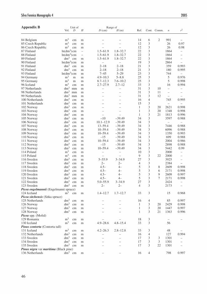
46
Silva Fennica Monographs 4 2005
84 Belgium m3 cm m – – 14 6 � 991 –85 czech Republic m3 cm m – – 1� 3 �6 0.9786 czech Republic m3 cm m – – 1� 3 �6 0.9887 Finland ln(dm3) cm – 1.5–61.9 1.8–3�.7 �� 3 1864 –88 Finland ln(dm3) cm – 1.5–61.9 1.8–3�.7 �� 3 1864 –89 Finland dm3 cm m 1.5–61.9 1.8–3�.7 �� 3 1864 –90 Finland ln(dm3) cm m – – 19 3 �864 –91 Finland dm3 cm m �–18 �–18 �1 3 359 0.9939� Finland dm3 cm m �–18 �–18 �1 3 180 0.99593 Finland ln(dm3) cm m 7–45 5–�9 �3 3 744 –94 Germany m3 m m 4.9–10.3 5–8.8 �5 3 5 0.97695 Germany m3 m m 8.7–1�.3 7.6–10.� �5 3 5 0.99896 Iceland m3 cm m �.7–�7.9 �.7–1� 33 3 16 0.99497 Netherlands dm3 mm m – – 31 3 10 – –98 Netherlands dm3 mm m – – 31 3 11 – –99 Netherlands dm3 mm m – – 31 3 1� – –100 Netherlands dm3 cm m – – 16 4 745 0.995101 Netherlands dm3 cm m – – 15 3 – –10� Norway dm3 cm m – – 1 3 �0 �6�1 0.998103 Norway dm3 cm m – – 1 3 �0 1348 0.998104 Norway dm3 cm m – – 1 3 �1 1813 0.996105 Norway dm3 cm m –10 –39.49 34 3 3597 0.988106 Norway dm3 cm m 10.1–1�.9 –39.49 34 3 – –107 Norway dm3 cm m 13–59.4 –39.49 34 3 7446 0.988108 Norway dm3 cm m 10–59.4 –39.49 34 3 6096 0.988109 Norway dm3 cm m 10–59.4 –39.49 34 3 1350 0.993110 Norway dm3 cm m –15 –39.49 34 3 699 0.988111 Norway dm3 cm m 10–59.4 –39.49 34 3 �004 0.98611� Norway dm3 cm m –15 –39.49 34 3 �898 0.988113 Norway dm3 cm m 10–59.4 –39.49 34 3 544� 0.99114 Poland m3 cm m – – 10 3 �000 –115 Poland m3 cm m – – 9 3 �� �000 –116 Sweden dm3 cm m 5–55.9 3–34.9 �7 3 39�5 –117 Sweden dm3 cm m �– �– 4 3 �384 –118 Sweden dm3 cm m 4.5– 4– 5 3 8 �609 0.998119 Sweden dm3 cm m 4.5– 4– 5 3 6 �171 0.9981�0 Sweden dm3 cm m 4.5– 4– 5 3 9 �609 0.9971�1 Sweden dm3 cm m 4.5– 4– 5 3 7 �171 0.9981�� Sweden dm3 cm m 5.0–55.9 3–34.9 �7 3 �4�4 –1�3 Sweden dm3 cm m �– �– 4 3 �173 –Picea engelmannii (Engelmanni spruce)1�4 Iceland m3 cm m 1.4–1�.7 1.7–1�.7 33 3 15 0.968Picea sitchensis (Sitka spruce)1�5 Netherlands dm3 cm m – – 16 4 85 0.9971�6 Norway dm3 cm m – – 1 3 �0 �4�9 0.9981�7 Norway dm3 cm m – – 1 3 �0 1447 0.9971�8 Norway dm3 cm m – – 1 3 �1 1363 0.996Picea spp. (Molid)1�9 Romania m3 cm m – – 18 3 – –130 Iceland m3 cm m 4.9–�8.6 4.8–15.4 33 3 56Pinus contorta (contorta tall)131 Iceland m3 cm m 4.�–�6.3 �.8–1�.8 33 3 48 –13� Netherlands dm3 cm m – – 16 4 1�7 0.994133 Sweden dm3 cm m – – 17 3 3 1301 –134 Sweden dm3 cm m – – 17 3 3 1301 –135 Sweden dm3 cm m – – 17 3 �� 1301 –Pinus nigra var maritima (Black pine)136 Netherlands dm3 cm m – – 16 4 798 0.997
Appendix B Unit of Range of Vol. D H D (cm) H (m) Ref. cont. comm. n r�

47
Zianis, Muukkonen, Mäkipää and Mencuccini Biomass and Stem Volume Equations for Tree Species in Europe
Pinus nigra var nigra (Black pine, Pin negru)137 Netherlands dm3 cm m – – 16 4 983 0.996138 Romania m3 cm m – – 18 3 – –Pinus spp.139 Germany m3 m – – �0 3 – –140 Germany m3 cm 5–75 – �0 3 – –141 Netherlands dm3 mm m – – 31 3 10 – –14� Netherlands dm3 mm m – – 31 3 11 – –143 Netherlands dm3 mm m – – 31 3 1� – –Pinus sylvestris (Scots pine, Mänty, Tall, Furu, Grove den, Pin silvestri)144 Austria dm3 dm dm 0.5– – �9 5 – –145 Belgium m3 cm – – – 36 8 – –146 Belgium m3 cm m – – 14 6 – –147 Finland ln(dm3) cm – 0.9–50.6 1.5–�8.3 �� 3 �050 –148 Finland ln(dm3) cm – 0.9–50.6 1.5–�8.3 �� 3 �050 –149 Finland dm3 cm m 0.9–50.6 1.5–�8.3 �� 3 �050 –150 Finland ln(dm3) cm m – – 19 3 �3�6 –151 Finland dm3 cm m �–18 �–18 �1 3 �49 0.99415� Finland dm3 cm m �–18 �–18 �1 3 486 0.989153 Finland dm3 cm m – – 35 3 1493 –154 Finland ln(dm3) cm m 7–50 5–�8 �3 3 1�91 –155 Germany m3 cm m 3–14 5.8–10.7 �4 3 – –156 Italy dm3 dm dm 13–49 7–�7.5 13 3 114 –157 Netherlands dm3 mm m – – 31 3 10 – –158 Netherlands dm3 mm m – – 31 3 11 – –159 Netherlands dm3 mm m – – 31 3 1� – –160 Netherlands dm3 cm m – – 16 4 1�07 0.994161 Norway dm3 cm m – – 1 3 �0 4816 0.99716� Norway dm3 cm m – – 1 3 �0 986 0.997163 Norway dm3 cm m – – 1 3 �1 3010 0.994164 Norway dm3 cm m 10– – 7 3 4356 0.996165 Norway dm3 cm m –1� – 7 3 �6�� 0.999166 Norway dm3 cm m –1� – 7 3 �6�� 0.999167 Norway dm3 cm m –1� – 7 3 �6�� 0.999168 Norway dm3 cm m –1� – 7 3 �6�� 0.999169 Romania m3 cm m – – 18 3 – –170 Sweden dm3 cm m 5–49.9 3–3�.9 �7 3 44�1 –171 Sweden dm3 cm m �– �– 4 3 3407 –17� Sweden dm3 cm m 4.5– 4– 5 3 8 3734 0.996173 Sweden dm3 cm m 4.5– 4– 5 3 6 ��15 0.996174 Sweden dm3 cm m 4.5– 4– 5 3 9 3734 0.993175 Sweden dm3 cm m 4.5– 4– 5 3 7 ��15 0.994176 Sweden dm3 cm m 5–49.9 3–3�.9 �7 3 �390 –177 Sweden dm3 cm m �– �– 4 3 �071 –Populus spp. (Poplar, Plop)178 Austria dm3 dm dm 5–10.4 – 3� 5 – 0.849179 Netherlands dm3 mm m – – 31 3 10 – –180 Netherlands dm3 mm m – – 31 3 11 – –181 Netherlands dm3 mm m – – 31 3 1� – –18� Romania m3 cm m – – 18 3 – –183 Romania m3 cm m – – 18 3 – –184 UK m3 cm m – – 8 � – –Populus tremula (Aspen, Plop tremulator)185 Norway dm3 cm m 13– – 11 9 – –186 Norway dm3 cm m 0–13 – 11 9 – –187 Romania m3 cm m – – 18 3 – –188 Sweden dm3 cm m – – 17 3 3 707 –189 Sweden dm3 cm m – – 17 3 3 707 –190 Sweden dm3 cm m – – 17 3 �� 707 –
Appendix B Unit of Range of Vol. D H D (cm) H (m) Ref. cont. comm. n r�

48
Silva Fennica Monographs 4 2005
Populus trichocarpa (Black cottonwood)191 Iceland m3 cm m 4.6–34 4.6–�0.7 33 3 �5 0.989Prunus avium (Wild cherry, Merisier, Zoete kers)19� Belgium m3 cm m – – 14 6 � 334 –Pseudotsuga menziesii (Douglas fir, Duglas)193 Belgium m3 cm m – – 14 6 � 63� –194 Netherlands dm3 cm m – – 16 4 1136 0.993195 Norway dm3 cm m 5– – 37 9 1 – –196 Romania m3 cm m – – 18 3 – –Pseudotsuga spp.197 Netherlands dm3 mm m – – 31 3 10 – –198 Netherlands dm3 mm m – – 31 3 11 – –199 Netherlands dm3 mm m – – 31 3 1� – –Quercus grisea (Gray oak, Stejar brumariu)�00 Romania m3 cm m – – 18 3 – –Quercus ilex (Holm oak)�01 Italy dm3 cm m 4.5–�6.1 6–16 6 3 �3 94 0.991�0� croatia m3 cm m 5–15 – 30 3 – –Quercus laevis (Turkey oak, cer)�03 Romania m3 cm m – – 18 3 – –Quercus pubescens (Downy oak, Stejar pufos)�04 croatia ln(m3) cm m 4.1–�3 3.5–15.1 � 3 347 0.96�05 croatia ln(m3) cm m 4.1–�3 3.5–15.1 � 3 �3 347 0.93��06 Romania m3 cm m – – 18 3 – –Quercus robur (Pedunculate oak)�07 Netherlands dm3 cm m – – 16 4 108 0.995Quercus rubra (Red oak, chêne rouge)�08 Belgium m3 cm m – – 14 6 � 891 –�09 Netherlands dm3 cm m – – 16 4 793 0.996Quercus spp. (Oak, chênes, Stejar)�10 Austria dm3 dm dm 1– – �9 5 – –�11 Austria dm3 dm dm 5–10.4 – 3� 5 – 0.64�1� Belgium m3 cm m – – 14 6 � �90 –�13 Netherlands dm3 mm m – – 31 3 10 – –�14 Netherlands dm3 mm m – – 31 3 11 – –�15 Netherlands dm3 mm m – – 31 3 1� – –�16 Romania m3 cm m – – 18 3 – –�17 UK m3 cm m – – 8 � – –Salix caprea (Goat willow, Salcie capreasca)�18 Norway dm3 cm m 5– – 3 9 – –�19 Romania m3 cm m – – 18 3 – –Salix spp. (Salcie)��0 Romania m3 cm m – – 18 3 – –��1 Romania m3 cm m – – 18 3 – –Sorbus aucuparia (Rowan)��� Norway dm3 cm m 5– – 3 9 – –Thuja pilicata (Western redcedar)��3 Netherlands dm3 cm m – – 16 4 165 0.993��4 Norway dm3 cm m 5– – 37 9 1 – –Tilia cordata (Tei)��5 Romania m3 cm m – – 18 3 – –Tsuga heterophylla (Hemlock)��6 Netherlands dm3 cm m – – 16 4 1�1 0.995��7 Norway dm3 cm m 5– – 37 9 1 – –Ulmus spp. (Elm, Orme, Ulm)��8 Belgium m3 cm m – – 14 6 � �76 –��9 Netherlands dm3 cm m – – 16 4 108 0.996�30 Romania m3 cm m – – 18 3 – –
Appendix B Unit of Range of Vol. D H D (cm) H (m) Ref. cont. comm. n r�

49
Zianis, Muukkonen, Mäkipää and Mencuccini Biomass and Stem Volume Equations for Tree Species in Europe
References – Appendix B
1 Bauger, E. 1995. Funksjoner og tabeller for kuber-ing av stående trær. Rapport fra Skogforsk(16): 1–�6.
� Benko, M., Novotny, V., Vrbek, B. & Szirovicza, l. �000. Volume tables of downy oak (Quercus pubescens Willd.). Radovi Sumarski Institut Jastre-barsko 8: 1–68.
3 Braastad, H. 1966. Volumtabeller for bjørk. Med-delelser fra det Norske Skogforsøksvesen �1(1): �3–78.
4 Brandel, G. 1974. Volymfunktioner för tall och gran. Skoghögskolan, Institutionen för skogsproduktion, Rapporter och Uppsatser 33: 178–191.
5 Brandel, G. 1990. Volumfunktioner för enskilda träd. Sveriges lantbruksuniversitet, Institutionen för skogsproduktion, Rapport �6: 1–181.
6 Brandini, P. & Tabacchi, G. 1996. Biomass and volume equations for holm oak and straberry-tree in coppice stands of Southern Sardinia. ISAFA communicazioni di Ricerca 96(1): 59–69.
7 Brantseg, A. 1967. Furu sønnafjells: kubering av stående skog, funksjoner og tabeller. Meddelelser fra det Norske Skogforsøksvesen 84: 689–739.
8 Broadmeadow, M. & Matthews, R. �004. Survey methods for Kyoto Protocol monitoring and veri-fication of UK forest carbon stocks. UK Emissions by Sources and Removals by Sinks due to land Use, land Use change and Forestry Activities, Report (June �004). cEH, Edinburgh.
9 Bruchwald, A. & Rymer-Dudzinska, T. 1987. Empirical equations for determining the volume of large timber of stem of growing spruce trees. Sylwan 131(5): 15–�0.
10 Bruchwald, A. 1987. Empirical formulas for determining the stem volume of standing spruce trees. Annals of Warsaw Agrivultural Universtity – SGGW-AR Forestry and Wood Technology 36: 57–60.
11 Børset, O. 1954. Kubering av osp på rot. Med-delelser fra det norske Skogforsøksvesen 1�: 391–447.
1� cerný, M. 1990. Biomass of Picea abies (l.) Karst. in midwestern Bohemia. Scandinavian Journal of Forest Research 5: 83–95.
13 corona, P. & Ferrara, A. 1987. Dendrometrical investigations on Pinus silvestris in Trentino-Alto Adige. Monti e Boschi 38(6): 51–54.
14 Dagnelie, P., Palm, R., Rondeux, J. & Thill, A.
1999. Tables de cubage des arbres et des peuple-ments forestiers. les Presses Agronomiques de Gembloux, Gembloux. 1�6 p.
15 De Vries, P.G. 1961. The principle of nomograms applied to the stem volume functions of the volume tables for forest trees grown in the Netherlands. Nederlands Bosbouw Tijdschrift 33(5): 114–1�1.
16 Dik, E.J. 1984. Estimating the wood volume of standing trees in forestry practice. Rijksinstituut voor onderzoek in de bos en landschapsbouw de Dorschkamp, Wageningen. Uitvoerige verslagen 19(1): 1–114.
17 Eriksson, H. 1973. Volymfunktioner för stående träd av ask, asp, klibbal och contorta-tall. Insti-tutionen för Skogsproduktion, Royal college of Forestry, Stockholm. Research Notes �6: 1–�6.
18 Giurgiu, V. 1974. O expresie matematica unica a relatiei diametru – înaltime – volum, pentru majori-tatea speciilor forestiere din Romania. Silvicultura si Exploatarea Padurilor 89(4): 173–178.
19 Hakkila, P. 1979. Wood density survey and dry weight tables for pine, spruce and birch stems in Finland. communicationes Instituti Forestalis Fenniae 96(3): 1–59.
�0 Hempel, G. 1968. Allometrische studie an Pinus cembra spp. sibirica (Rupr.) Kryl. und Abies sibirica (ledeb.). Archiv für Forstwesen 17(11): 1099–1115.
�1 Kanninen, K., Uusvaara, O. & Valonen, P. 1979. Kokopuuraaka-aineen mittaus ja ominaisuudet. Folia Forestalia 403: 1–53.
�� laasasenaho, J. 198�. Taper curve and volume functions for pine, spruce and birch. communica-tiones Instituti Forestalis Fenniae 108: 1–74.
�3 laasasenaho, J. & Sevola, Y. 1971. Mänty- ja kuusi-runkojen puutavarasuhteet ja kantoarvot. com-municationes Instituti Forestalis Fenniae 74(3): 1–87.
�4 lockow, K.-W. 1993. Modellbildung und quanti-fizierung der durchmesser- und volumenstruktur des ausscheidenden kieferjungbestandes – holz-meßkundliche entscheideungshilfen für die erst-durchforstung. Beiträge für Forstwirtschaft und landschaftsökologie �7(�): 77–8�.
�5 Mund, M., Kummetz, E., Hein, M., Bauer, G.A. & Schulze, E.-D. �00�. Growth and carbon stocks of a spruce forest chronosequence in central Europe. Forest Ecology and Management 171: �75–�96.
�6 Norrby, M. 1990. Volym- och formtalsfunktioner for larix sukaczewii och larix sibirica på Island.

50
Silva Fennica Monographs 4 2005
Institutionen för skogsskötsel. Series Volym- och formtalsfunktioner for larix sukaczewii och larix sibirica på Island. Sveriges lantbruksuniversitet, Umeå.
�7 Näslund, M. 1947. Funktioner och tabeller för kubering av stående träd. Meddelanden från Statens skogsforskningsinstitutet 36(3): 1–81.
�8 Pellinen, P. 1986. Biomasseuntersuchungen im Kalkbuchenwald. University of Göttingen, Ger-many. 145 p.
�9 Pollanschütz, J. 1974. Formzahlfunktionen der Hauptbaumarten Österreichs. Allgemeine Forstzei-tung 85: 341–343.
30 Pranjic, A. & lukic, N. 1986. Form factor and volume table for Holm oak (Quercus ilex l.). Glasnik za Sumske Pokuse, Posebno Izdanje �: 169–177.
31 Schelhaas, M.J., Nabuurs, G.J., Jans, W.W.P., Moors, E.J., Sabaté, S. & Daamen, W.P. �00�. converging estimates of the forest carbon sink. Alterra-rapport 631: 1–44.
3� Schieler, K. 1988. Diploma thesis, Institute for Forest growth and Yield Reserch, University for Agricultural Sciences, Vienna.
33 Snorrason, A. & Einarsson, S.F. �004. Single-tree biomass and stem volume functions for eleven tree species used in Icelandic forestry. Submitted manuscript.
34 Vestjordet, E. 1967. Funksjoner og tabeller for kubering av stående gran. Meddelelser fra det Norske Skogforsøksvesen 84: 539–574.
35 Vuokila, Y. 1965. Functions for variable density yield tables of pine based on temporary sample plots. communicationes Instituti Forestalis Fenniae 60(4): 1–86.
36 Xiao, c.W., curiel Yuste, J., Janssens, I.A., Roskams, P., Nachtergale, l., carrara, A., Sanchez, B.Y. & ceu-lemans, R. �003. Above-and belowground biomass and net primary production in a 73-year-old Scots pine forest. Tree Physiology �3: 505–516.
37 Øen, S., Bauger, E. & Øyen, B.-H. �001. Func-tionar for volumberekning av framande treslag i Vest-Norge. Aktuelt fra Skogforsk 3/01: 18–19.

51
Zianis, Muukkonen, Mäkipää and Mencuccini Biomass and Stem Volume Equations for Tree Species in Europe
Contact persons – Appendix B
1 Joosten R., [email protected], Univertsity Paderborn, Germany
� Matthews, R., [email protected], Forest Research, Alice Holt Research Station, UK
3 Muukkonen P., [email protected], Finnish Forest Research Institute, Finland
4 Nabuurs G.-J., [email protected], Alterra, Wageningen, the Netherlands
5 Prskawetz M., [email protected], Federal Office and Research centre for Forests, Vienna, Austria
6 Sheridan M., [email protected] , Depart-ment of Plant Biology, Gembloux agricultural University, Belgium
7 Snorrason A., [email protected], Skógrækt ríki-sins, Iceland
8 Xiao C.W., [email protected], University of Antwerpen, Belgium
9 Zianis D., TEI Kavalas, Greece
Comments – Appendix B
1 Plantations� Stem volume to upper girth limit of �� cm3 Including bark4 Excluding bark5 Merchantable volume >34 cm6 Including bark, Southern Sweden, adjusted r�
7 Excluding bark, Southern Sweden, adjusted r�
8 Including bark, Northern Sweden, adjusted r�
9 Excluding bark, Northern Sweden, adjusted r�
10 Dominant11 Dominated1� Seed trees13 Merchantable wood >7 cm14 Non merchantable wood <7 cm15 Including bark, trees without forks16 Including bark, forked trees17 Excluding bark, trees without forks18 Excluding bark, forked trees19 Without bark�0 Tree height 4 m and more�1 Tree height over 10 m�� Merchantable volume�3 Merchantable volume, >3–4 cm

5�
Silva Fennica Monographs 4 2005
Appendix C. Volume equations for different tree species. The format of the stem volume equation (where D is diameter and H is height) is given in the column labelled Equation, and a–g are parameter values. The “ln” is the natural logarithm and the “log” is the 10-based logarithm.
Equation
Abies alba (Silver fir)1 Norway a·Hb·Dc·(H–1.3)d·(D+100)e
Abies grandis (Grand fir)� Netherlands Da·Hb·exp(c)3 Norway a·Hb·Dc·(H–1.3)d·(D+100)e
Abies sibirica (Fir)4 Germany a·Db
Abies spp. (Fir, Brad)5 Austria (π/4)·(a·D�·H+b·D�·H·ln(D)�+c·D�+d·D·H+e·H+f·D+g6 Austria (π/4)·(a·D�·H+b·D�·H·ln(D)�+c·D�+d·D·H7 Romania a·10(b·log(D)+c·log(D)^�+d·log(H)+e·log(H)^�)
Acacia spp. (Salcim)8 Romania a·10(b·log(D)+c·log(D)^�+d·log(H)+e·log(H)^�)
Acer pseudoplatanus (Maple, Erable sycomore, Paltin, Sycamore)9 Belgium a+b·D+c·D�+d·D3+e·H+f·D�·H10 Netherlands Da·Hb·exp(c)11 Romania a·10(b·log(D)+c·log(D)^�+d·log(H)+e·log(H)^�)
1� UK a+b·D�·Hc
Alnus alba (Anin alb)13 Romania a·10(b·log(D)+c·log(D)^�+d·log(H)+e·log(H)^�)
Alnus glutinosa (Black alder, Klibbal)14 Netherlands Da·Hb·exp(c)15 Norway a+b·D�+c·D�·H16 Norway a+b·D�+c·D�·H+d·H�·D17 Sweden a·D�+b·D�·H+c·D·H�+d·D·H+e·D�H�
18 Sweden a·Db·Hc
19 Sweden a·D�+b·D�·H+c·D·H�+d·D·H+e·D�H�
Alnus incana (Grey alder)�0 Norway a+b·D�+c·D�·H+d·H�·D+e·H�
Alnus nigra (Anin negru)�1 Romania a·10(b·log(D)+c·log(D)^�+d·log(H)+e·log(H)^�)
Alnus spp. (Alder)�� Austria (π/4)·(a·D�·H+b·D�+c·D)Arbutus unedo (Strawberry–tree)�3 Italy a+b·D�
Betula pendula (Birch, Berk)�4 Netherlands Da·Hb·exp(c)Betula spp. (Birch, Björk, Bjørk, Bouleaux, Mesteacan)�5 Belgium a+b·D+c·D�+d·D3+e·H+f·D�·H�6 Finland a+b·ln(D)�7 Finland a+b·ln(c+d·D)+e·D�8 Finland a·(Db)·(cD)·(Hd)·(H–1.3)e
�9 Finland a+b·ln(D)+c·ln(H)+d·ln(H–1.3)+e·D30 Norway a+b·D�+c·D�·H+d·D·H�+e·H�
31 Norway a+b·D�+c·D�·H+d·D·H�+e·H�
3� Romania a·10(b·log(D)+c·log(D)^�+d·log(H)+e·log(H)^�)
33 Sweden a·D�+b·D�·H+c·D·H�+d·H�
34 Sweden 10a·Db·(D+�0)c·Hd·(H–1.3)e
35 Sweden 10a·Db·(D+�0)c·Hd·(H–1.3)e
36 Sweden 10a·Db·(D+�0)c·Hd·(H–1.3)e

53
Zianis, Muukkonen, Mäkipää and Mencuccini Biomass and Stem Volume Equations for Tree Species in Europe
Parameters a b c d e f g
1 1.666� 3.�394 1.9334 –1.8997 –0.9739 – –
� 1.77��0 0.96736 –�.45��4 – – – –3 1.666� 3.�394 1.9334 –1.8997 –0.9739 – –
4 0.0001316 �.5� – – – – –
5 0.580��3 –0.0307373 –17.1507 0.089869 –0.080557 19.661 –�.45846 0.560673 0.15468 –0.65583 0.033�10 – – –7 4.5�·10–5 �.1554 –0.1067 0.9380 0.0��8 – –
8 0.00046903 1.807 0.0�9� –0.4155 0.5455 – –
9 0.010343 –0.00450536 3.4070·10–4 –4.047�·10–6 7.7115·10–4 �.9836·10–5 –10 1.89756 0.97716 –�.94�53 – – – –11 0.00035375 1.0� 0.3997 0.666 0.0�1 – –1� –0.01�668 0.0000737 0.75 – – – –
13 0.00065013 1.6750 0.1001 –0.4990 0.590� – –
14 1.85749 0.88675 –�.5��� – – – –15 8.65�4 0.076844 0.031573 – – – –16 0.6716 0.75708 0.0�9679 0.004341 – – –17 0.19�6 0.01631 0.003755 –0.0�756 0.000499 – –18 0.05437 1.94505 0.9�947 – – – –19 0.��64 0.01347 0.007665 –0.06669 0.0004�8 – –
�0 –1.868�7 0.�1461 0.01�83 0.0138 –0.06311 – –
�1 8.666·10–5 1.7148 0.1014 0.801 0.0530 – –
�� 0.387399 7.171�3 0.04407 – – – –
�3 –0.5547 0.3757 – – – – –
�4 1.89060 .�6595 –1.07055 – – – –
�5 –0.01139� –0.00031447 0.000�79�11 –5.7966·10–6 –5.9573·10–4 3.0409·10–5 –�6 –�.09787 �.55058 – – – – –�7 –5.41948 3.57630 � 1.�5 –0.0395855 – –�8 0.011197 �.10�53 0.986 3.98519 –�.65900 – –�9 –4.4759 �.0851 4.0691 –�.7375 –0.013311 – –30 –1.868�7 0.�1461 0.01�83 0.01380 0.06311 – –31 0.99983 0.0063�5 0.0�849 0.00885 –0.00799 – –3� 8.141·10–5 �.�48 –0.�06� 0.1946 0.4147 – –33 0.1305 0.01338 0.01757 –0.05606 – – –34 –0.89359 �.�7954 –1.1867� 7.0736� –5.45175 – –35 –0.93631 �.30�1� –1.40378 8.01817 –6.188�5 – –36 –0.44��4 �.47580 –1.40854 5.16863 –3.77147 – –

54
Silva Fennica Monographs 4 2005
37 Sweden 10a·Db·(D+�0)c·Hd·(H–1.3)e
38 Sweden a·D�+b·D�·H+c·D·H�+d·H�
39 UK a+b·D�·Hc
Carpinus spp.40 Netherlands a·D(b+c)·Hd
41 Netherlands a·D(b+c)·Hd
4� Netherlands a·D(b+c)·Hd
Chamaecyparis lawsoniana (lawson cypress)43 Netherlands Da·Hb·exp(c)Corylus avellana (Hazel)44 Norway a+b·D�+c·D�·H+d·D·H�+e·H�
Fagus spp. (Beech, Fag)45 Austria (π/4)·(a·D�·H+b·D�·H·ln(D)�+c·D�+d·D·H+e·H+f·D+g)46 Austria (π/4)·(a·D�·H+b·D�+c·D)47 Romania a·10(b·log(D)+c·log(D)^�+d·log(H)+e·log(H)^�)
48 UK a+b·D�·Hc
Fagus sylvatica (Beech, Rotbuche, Beuk)49 Belgium a+b·D+c·D�+d·D3+e·H+f·D�·H50 Germany a+b·D·H�+c·D3
51 Germany a+b·D·H�+c·D3
5� Netherlands Da·Hb·exp(c)53 Netherlands a·Db·Hc
Fraxinus exselsior (Ash, Frêne, Es)54 Belgium a+b·D+c·D�+d·D3+e·H+f·D�·H55 Netherlands Da·Hb·exp(c)56 Sweden a·D�·H+b·D�+c·D·H57 Sweden a·D�·H+b·D�+c·D·H58 Sweden a·Db·Hc
59 Sweden a·D�·H+b·D�+c·D·H60 Sweden a·D�·H+b·D�+c·D·HFraxinus spp. (Ash)61 Norway a+b·D�+c·D�·H+d·D·H�+e·H�
6� Romania a·10(b·log(D)+c·log(D)^�+d·log(H)+e·log(H)^�)
63 UK a+b·D�·Hc
Larix decidua (larch, Mélèzes)64 Austria (π/4)·(a·D�·H+b·D�·H·ln(D)�+c·D�+d·D·H+e·H+f·D+g)65 Austria (π/4)·(a·D�·H+b·D�+c·D)66 Belgium a+b·D+c·D�+d·D3+e·H+f·D�·H67 Netherlands Da·Hb·exp(c)68 Norway a·Hb·Dc·(H–1.3)d·(D+100)e
Larix hybrid (Hyprid larix)69 Norway a·Hb·Dc·(H–1.3)d·(D+100)e
Larix kaempferi (Japanese larch)70 Netherlands Da·Hb·exp(c)71 Norway a·Hb·Dc·(H–1.3)d·(D+100)e
Larix sibirica (Siberian larix)7� Iceland exp(a)·Db·Hc
73 Iceland exp(a)·Db·Hc
74 Iceland a·Db·Hc
75 Norway a·Hb·Dc·(H–1.3)d·(D+100)e
Larix spp. (lehtikuusi, lork, larice)76 Finland a+b·D�+c·D�·H+d·H�·D77 Finland a+b·D�+c·D�·H+d·H�·D
Appendix C. Volume equations (cont.)
Equation

55
Zianis, Muukkonen, Mäkipää and Mencuccini Biomass and Stem Volume Equations for Tree Species in Europe
37 –0.35394 �.5�141 –1.54�57 4.88165 –3.474�� – –38 0.143� 0.008561 0.0�180 –0.06630 – – –39 –0.009184 0.0000673 0.75 – – – –
40 0.000�1491 �.�58957614 0.001411006 0.60�91075 – – –41 0.000�1491 �.�58957614 –0.011�0638 0.60�91075 – – –4� 0.000�1491 �.�58957614 –0.00956695 0.60�91075 – – –
43 1.85�98 .86717 –�.33706 – – – –
44 –1.868�7 0.�1461 0.01�83 0.0138 –0.06311 – –
45 0.989�53 –0.0371508 –31.0674 –0.3863�1 0.�1946� 49.6136 –��.37�46 0.517300 –13.6�144 9.9888 – – – –47 0.0000757 1.3791 0.�1�7 1.199� –0.0584 – –48 –0.014306 0.0000748 0.75 – – – –
49 –0.01557� 0.00�90013 –7.0476·10–6 �.393·10–06 –0.00135�8 3.9837·10–5 –50 15.589·10–3 0.01696·10–3 0.01883·10–3 – – – –51 16.641·10–3 0.7�179·10–3 0.00�5�·10–3 – – – –5� 1.55448 1.55880 –3.57875 – – – –53 0.049 1.78189 1.08345 – – – –
54 –0.039836 0.006�6�765 –0.00015937 –1.990�·10–7 –0.0009834 3.787�·10–5 –55 1.95�77 0.77�06 –�.48079 – – – –56 0.03�46 0.03310 0.041�7 – – – –57 0.03593 0.03310 0.041�7 – – – –58 0.063�8 1.9�4�8 0.88690 – – – –59 0.03�49 0.0�941 0.0389� – – – –60 0.03453 0.0�941 0.0389� – – – –
61 –1.868�7 0.�1461 0.01�83 0.0138 –0.06311 – –6� 0.00030648 1.�676 0.310� 0.49�9 0.096� – –63 –0.01�107 0.0000777 0.75 – – – –
64 0.609443 –0.0455748 –18.6631 –0.�48736 0.1�6594 36.9783 –14.�0465 0.487�70 –�.04�91 5.9995 – – – –66 –0.03088 0.004676�61 –4.8614·10–5 –3.8178·10–6 –0.0011638 4.0597·10–5 –67 1.86670 1.08118 –3.0488 – – – –68 0.7761 3.6461 1.9166 –�.3179 –0.8�36 – –
69 0.7761 3.6461 1.9166 –�.3179 –0.8�36 – –
70 1.87077 1.00616 –�.8748 – – – –71 0.7606 3.5377 1.9741 –�.190� –0.8459 – –
7� –�.5079 1.7574 0.9808 – – – –73 –�.9946 1.8105 0.9908 – – – –74 0.0983 1.551 1.1483 – – – –75 0.7761 3.6461 1.9166 –�.3179 –0.8�36 – –0.7761 3.6461 1.9166 –�.3179 –0.8�36 – –
76 0.5 0.0753 0.03345 –0.00�43 – – –77 0.4 –0.01 0.03355 –0.00359 – – –
Parameters a b c d e f g

56
Silva Fennica Monographs 4 2005
78 Netherlands a·D(b+c)·Hd
79 Netherlands a·D(b+c)·Hd
80 Netherlands a·D(b+c)·Hd
81 Romania a·10(b·log(D)+c·log(D)^�+d·log(H)+e·log(H)^�)
Picea abies (Norway spruce, Kuusi, Gran, Epicéa, Fijnspar)8� Austria (π/4)·(a·D�·H+b·D�·H·ln(D)�+c·D�+d·D·H+e·H+f·D)83 Austria (π/4)·(a·D�·H+b·D�·H·ln(D)�+c·D�+d·D)84 Belgium a+b·D+c·D�+d·D3+e·H+f·D�·H85 czech Republic a·Db
86 czech Republic a·(H·D�)b
87 Finland a+b·ln(D)88 Finland a+b·ln(c+d·D)+e·D89 Finland a·(Db)·(cD)·(Hd)·(H–1.3)e
90 Finland a+b·ln(D)+c·ln(H)+d·ln(H–1.3)+e·D91 Finland a·Db·Hc
9� Finland a·Db·Hc
93 Finland a+b·ln(D)+c·D�
94 Germany a·H·D�
95 Germany a·H·D�
96 Iceland a·Db·Hc
97 Netherlands a·D(b+c)·Hd
98 Netherlands a·D(b+c)·Hd
99 Netherlands a·D(b+c)·Hd
100 Netherlands Da·Hb·ec
101 Netherlands a·Db·Hc
10� Norway a·Hb·Dc·(H–1.3)d·(D+40)e
103 Norway a·Hb·Dc·(H–1.3)d·(D+40)e
104 Norway a·Hb·Dc·(H–1.3)d·(D+40)e
105 Norway a+b·D�·H+c·D·H�+d·H�+e·D·H106 Norway a+b·D·H�+c·H�+d·D·H+e·H+f·D107 Norway a+b·D�·H+c·D·H�+d·H�+e·D·H108 Norway a+b·D�·H+c·D·H�+d·H�+e·D·H109 Norway a+b·D�·H+c·D·H�+d·H�+e·D·H110 Norway a+b·D�·H+c·D·H�+d·D�
111 Norway a+b·D�·H+c·D·H�+d·H�+e·D·H11� Norway a+b·D�·H+c·D·H�+d·H�+e·D·H113 Norway a+b·D�·H+c·D·H�+d·H�+e·D·H114 Poland (π/40000)·H·D·(a+b·D)115 Poland (π/40000)·H·D·(a·D+b)116 Sweden a·D�+b·D�·H+c·D·H�+d·H�
117 Sweden 10a·Db·(D+�0)c·Hd·(H–1.3)e
118 Sweden 10a·Db·(D+�0)c·Hd·(H–1.3)e
119 Sweden 10a·Db·(D+�0)c·Hd·(H–1.3)e
1�0 Sweden 10a·Db·(D+�0)c·Hd·(H–1.3)e
1�1 Sweden 10a·Db·(D+�0)c·Hd·(H–1.3)e
1�� Sweden a·D�+b·D�·H+c·D·H�+d·H�
1�3 Sweden 10a·Db·(D+�0)c·Hd·(H–1.3)e
Picea engelmannii (Engelmanni spruce)1�4 Iceland a·Db·Hc
Picea sitchensis (Sitka spruce)1�5 Netherlands Da·Hb·exp(c)1�6 Norway a·Hb·Dc·(H–1.3)d·(D+40)e
1�7 Norway a·Hb·Dc·(H–1.3)d·(D+40)e
Appendix C. Volume equations (cont.)
Equation

57
Zianis, Muukkonen, Mäkipää and Mencuccini Biomass and Stem Volume Equations for Tree Species in Europe
78 0.00035�17 �.1�8418�8 0.003�9�718 0.76�839�5 – – –79 0.00035�17 �.1�8418�8 –0.1054168 0.76�839�5 – – –80 0.00035�17 �.1�8418�8 –0.00�6067 0.76�839�5 – – –81 �.8��·10–5 �.�060 –0.1136 1.115 0.01�9 – –
8� 0.46818 –0.013919 –�8.�13 0.37474 –0.�8875 �8.�79 –83 0.563443 –0.1�731 –8.550�� 7.6331 – – –84 –0.0109�9 0.004380951 –9.4713·10–5 –7.80�4·10–6 –0.00�79�� 4.8346·10–5 –85 0.00059707 �.1�86 – – – – –86 0.00011�61 0.8785� – – – – –87 –�.41�18 �.6�463 – – – – –88 –5.39934 3.46468 � 1.�5 –0.0�73199 – –89 0.0��9�7 1.91505 0.99146 �.8�541 –1.53547 – –90 –3.7544 1.8960 �.8979 –1.60�0 –0.0078�7 – –91 0.7877 1.930� 0.79465 – – – –9� 0.10838 1.8�0� 0.77154 – – – –93 –�.59385 �.71757 –0.000097 – – – –94 0.50� – – – – – –95 0.418 – – – – – –96 0.1�99 1.6834 0.8598 – – – –97 0.00053�38 �.1641�6647 0.004108377 0.54879808 – – –98 0.00053�38 �.1641�6647 –0.04670018 0.54879808 – – –99 0.00053�38 �.1641�6647 –0.010�58� 0.54879808 – – –100 1.75055 1.10897 –�.75863 – – – –101 0.04143 1.6704 1.3337 – – – –10� 0.6844 3.0�96 �.0560 –1.7377 –0.9756 – –103 0.7464 �.496 �.0714 –1.4175 –0.9601 – –104 0.58�4 1.1987 1.9339 –0.0594 –0.744� – –105 0.5� 0.0�403 0.01463 –0.10983 0.15195 – –106 –31.57 0.0016 0.0186 0.63 –�.34 3.� –107 10.14 0.01�4 0.03117 –0.36381 0.�8578 – –108 6.69 0.01308 0.0�853 –0.31956 0.�8969 – –109 0.46 0.0�4�7 0.015�1 –0.18�54 0.�0994 – –110 0.67 0.030�3 0.0071� 0.04175 – – –111 0.�8 0.00815 0.03053 –0.507�5 0.51643 – –11� 0.3 0.0�593 0.01�68 –0.0977 0.14586 – –113 4.33 0.01491 0.0�606 –0.31854 0.31106 – –114 0.666151 0.458507 – – – – –115 0.53005 1.��9�83 – – – – –116 0.1150 0.01746 0.0�0�� –0.05618 – – –117 –0.9513 1.9781 –0.5�54 �.7604 –1.4684 – –118 –0.79783 �.07157 –0.7388� 3.1633� –1.8�6�� – –119 –1.0�039 �.001�8 –0.47473 �.87138 –1.61803 – –1�0 –0.8��49 �.11094 –0.896�6 3.5181� –�.05567 – –1�1 –1.06019 �.04�39 –0.54�9� �.80843 –1.5�110 – –1�� 0.1104 0.019�5 0.01815 –0.04936 – – –1�3 –1.034� 1.9683 –0.3850 �.4018 –1.�075 – ––1.034� 1.9683 –0.3850 �.4018 –1.�075 – –
1�4 0.4693 1.311 0.781 – – – –
1�5 1.78383 1.13397 –�.90893 – – – –1�6 0.1614 3.7060 1.9747 –�.�905 –0.6665 – –1�7 0.1870 3.7077 1.9854 –�.�816 –0.7161 – –
Parameters a b c d e f g
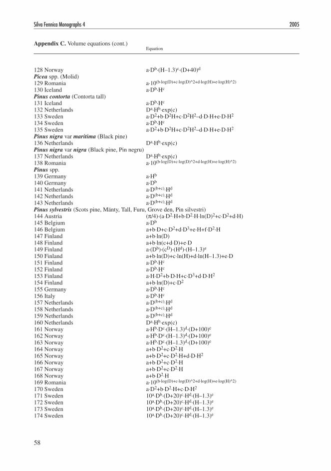
58
Silva Fennica Monographs 4 2005
1�8 Norway a·Db·(H–1.3)c·(D+40)d
Picea spp. (Molid)1�9 Romania a·10(b·log(D)+c·log(D)^�+d·log(H)+e·log(H)^�)
130 Iceland a·Db·Hc
Pinus contorta (contorta tall)131 Iceland a·Db·Hc
13� Netherlands Da·Hb·exp(c)133 Sweden a·D�+b·D�H+c·D�H�–d·D·H+e·D·H�
134 Sweden a·Db·Hc
135 Sweden a·D�+b·D�H+c·D�H�–d·D·H+e·D·H�
Pinus nigra var maritima (Black pine)136 Netherlands Da·Hb·exp(c)Pinus nigra var nigra (Black pine, Pin negru)137 Netherlands Da·Hb·exp(c)138 Romania a·10(b·log(D)+c·log(D)^�+d·log(H)+e·log(H)^�)
Pinus spp.139 Germany a·Hb
140 Germany a·Db
141 Netherlands a·D(b+c)·Hd
14� Netherlands a·D(b+c)·Hd
143 Netherlands a·D(b+c)·Hd
Pinus sylvestris (Scots pine, Mänty, Tall, Furu, Grove den, Pin silvestri)144 Austria (π/4)·(a·D�·H+b·D�·H·ln(D)�+c·D�+d·H)145 Belgium a·Db
146 Belgium a+b·D+c·D�+d·D3+e·H+f·D�·H147 Finland a+b·ln(D)148 Finland a+b·ln(c+d·D)+e·D149 Finland a·(Db)·(cD)·(Hd)·(H–1.3)e
150 Finland a+b·ln(D)+c·ln(H)+d·ln(H–1.3)+e·D151 Finland a·Db·Hc
15� Finland a·Db·Hc
153 Finland a·H·D�+b·D·H+c·D3+d·D·H�
154 Finland a+b·ln(D)+c·D�
155 Germany a·Db·Hc
156 Italy a·Db·Hc
157 Netherlands a·D(b+c)·Hd
158 Netherlands a·D(b+c)·Hd
159 Netherlands a·D(b+c)·Hd
160 Netherlands Da·Hb·exp(c)161 Norway a·Hb·Dc·(H–1.3)d·(D+100)e
16� Norway a·Hb·Dc·(H–1.3)d·(D+100)e
163 Norway a·Hb·Dc·(H–1.3)d·(D+100)e
164 Norway a+b·D�+c·D�·H165 Norway a+b·D�+c·D�·H+d·D·H�
166 Norway a+b·D�+c·D�·H167 Norway a+b·D�+c·D�·H168 Norway a+b·D�·H169 Romania a·10(b·log(D)+c·log(D)^�+d·log(H)+e·log(H)^�)
170 Sweden a·D�+b·D�·H+c·D·H�
171 Sweden 10a·Db·(D+�0)c·Hd·(H–1.3)e
17� Sweden 10a·Db·(D+�0)c·Hd·(H–1.3)e
173 Sweden 10a·Db·(D+�0)c·Hd·(H–1.3)e
174 Sweden 10a·Db·(D+�0)c·Hd·(H–1.3)e
Appendix C. Volume equations (cont.) Equation

59
Zianis, Muukkonen, Mäkipää and Mencuccini Biomass and Stem Volume Equations for Tree Species in Europe
1�8 0.�101 1.89�0 1.1095 –0.3895 – – –
1�9 0.00009464 1.9341 –0.07�� 0.6365 0.17� – –130 0.0739 1.7508 1.0��8 – – – –
131 0.1491 1.6466 0.83�5 – – – –13� 1.89303 0.98667 –�.88614 – – – –133 0.11�1 0.0�870 –0.000061 0.09176 0.01�49 – –134 0.04514 1.9005 1.06964 – – – –135 0.0883 0.03�0� –0.000114 –0.0789� 0.01049 – –
136 1.8919� 0.95374 –�.7�505 – – – –
137 1.95645 0.88671 –�.7675 – – – –138 0.0001089� 1.9701 0.010� 0.4858 0.1330 – –
139 0.000074 3.1 – – – – –140 0.0001078 �.56 – – – – –141 0.0004�613 �.066��5947 –0.0019�6657 0.80636901 – – –14� 0.0004�613 �.066��5947 –0.07956�44 0.80636901 – – –143 0.0004�613 �.066��5947 0.00369501 0.80636901 – – –
144 0.435949 –0.0149083 5.�1091 0.0�870� – – –145 0.000�44 �.3�716 – – – – –146 –0.039836 4.8710·10–3 –6.10�8·10–5 1.4889·10–5 7.3997·10–5 �.9��1·10–5 –147 –�.�945 �.570�5 – – – – –148 –5.39417 3.48060 � 1.�5 –0.039884 – –149 0.036089 �.01395 0.99676 �.070�5 –1.07�09 – –150 –3.�890 1.9995 �.1395 –1.1411 –0.00�847 – –151 0.094� 1.9671 0.7005 – – – –15� 0.095 1.9185 0.7381 – – – –153 0.0578� 0.1163� –0.0109� –0.01317 – – –154 –�.3791� �.6�903 –0.0001�6 – – – –155 5.6537·10–5 1.960466 0.894433 – – – –156 1.480589 1.98�459514 0.74�674501 – – – –157 0.00�07765 1.95�76440� –8.6651E–05 0.48560878 – – –158 0.00�07765 1.95�76440� –0.11110535 0.48560878 – – –159 0.00�07765 1.95�76440� 0.001095496 0.48560878 – – –160 1.8�075 1.074�7 –�.8885 – – – –161 0.14�4 �.0786 1.90�8 –1.0�59 –0.�640 – –16� 0.1�63 �.46�1 1.9008 –1.3716 –0.�663 – –163 0.4434 4.9667 1.991� –3.661� –0.750� – –164 8.65�4 0.076844 0.031573 – – – –165 0.6716 0.075708 0.0�9679 – – – –166 �.0044 0.0�9886 0.03697� 0.004341 – – –167 �.91�1 0.039994 –0.001091 – – – –168 �.9361 0.038906 – – – – –169 0.00014808 1.8341 –0.0448 0.3115 0.35�5 – –170 0.10�8 0.0�705 0.005�15 – – – –171 –1.1��6 �.0180 –0.�135 1.8�71 –0.8�97 – –17� –1.�0914 1.94740 –0.05947 1.40958 –0.45810 – –173 –1.38903 1.84493 0.06563 �.0�1�� –1.01095 – –174 –1.�5�46 1.98�44 –0.13118 1.03781 –0.0348� – –
Parameters a b c d e f g

60
Silva Fennica Monographs 4 2005
175 Sweden 10a·Db·(D+�0)c·Hd·(H–1.3)e
176 Sweden a·D�+b·D�·H+c·D·H�
177 Sweden 10a·Db·(D+�0)c·Hd·(H–1.3)e
Populus spp. (Poplar, Plop)178 Austria (π/4)·(a·D�·H+b·D�+c·D)179 Netherlands a·D(b+c)·Hd
180 Netherlands a·D(b+c)·Hd
181 Netherlands a·D(b+c)·Hd
18� Romania a·10(b·log(D)+c·log(D)^�+d·log(H)+e·log(H)^�)
183 Romania a·10(b·log(D)+c·log(D)^�+d·log(H)+e·log(H)^�)
184 UK a+b·D�·Hc
Populus tremula (Aspen, Plop tremulator)185 Norway a+b·D�·H186 Norway a+b·D�·H187 Romania a·10(b·log(D)+c·log(D)^�+d·log(H)+e·log(H)^�)
188 Sweden a·D�+b·D�·H+c·D�H�+d·D·H+e·D·H�
189 Sweden a·Db·Hc
190 Sweden a·D�·H+b·D�·H+c·D�H�+d·D·H+e·D·H�
Populus trichocarpa (Black cottonwood)191 Iceland a·Db·Hc
Prunus avium (Wild cherry, Merisier, Zoete kers)19� Belgium a+b·D+c·D�+d·D3+e·H+f·D�·HPseudotsuga menziesii (Douglas fir, Duglas)193 Belgium a+b·D+c·D�+d·D3+e·H+f·D�·H194 Netherlands Da·Hb·exp(c)195 Norway a·Hb·Dc·(H–1.3)d·(D+40)e
196 Romania a·10(b·log(D)+c·log(D)^�+d·log(H)+e·log(H)^�)
Pseudotsuga spp.197 Netherlands a·D(b+c)·Hd
198 Netherlands a·D(b+c)·Hd
199 Netherlands a·D(b+c)·Hd
Quercus grisea (Gray oak, Stejar brumariu)�00 Romania a·10(b·log(D)+c·log(D)^�+d·log(H)+e·log(H)^�)
Quercus ilex (Holm oak)�01 Italy a+b·D�·H�0� croatia a·D a·Db·Hc
Quercus laevis (Turkey oak, cer)�03 Romania a·10(b·log(D)+c·log(D)^�+d·log(H)+e·log(H)^�)
Quercus pubescens (Downy oak, Stejar pufos)�04 croatia a+b·ln(D)+c·H a+b·ln(D)+c·H�05 croatia a+b·ln(D)+c·H a+b·ln(D)+c·H�06 Romania a·10(b·log(D)+c·log(D)^�+d·log(H)+e·log(H)^�)
Quercus robur (Pedunculate oak)�07 Netherlands Da·Hb·exp(c)Quercus rubra (Red oak, chêne rouge)�08 Belgium a+b·D+c·D�+d·D3+e·H+f·D�·H�09 Netherlands Da·Hb·exp(c)Quercus spp. (Oak, chênes, Stejar)�10 Austria (π/4)·(a·D�·H+b·D�+c·D·H+d·H+e·D+f)�11 Austria (π/4)·(a·D�·H+b·D�·H·ln(D)�+c·D�)�1� Belgium a+b·D+c·D�+d·D3+e·H+f·D�·H�13 Netherlands a·D(b+c)·Hd
�14 Netherlands a·D(b+c)·Hd
Appendix C. Volume equations (cont.)
Equation

61
Zianis, Muukkonen, Mäkipää and Mencuccini Biomass and Stem Volume Equations for Tree Species in Europe
175 –1.5�761 1.8�9�8 0.07454 1.4379� –0.35559 – –176 0.107� 0.0�4�7 0.007315 – – – –177 –1.�605 1.93�� –0.0897 �.1795 –1.1676 – –
178 0.366419 1.133�3 0.1306 – – – –179 0.0009507 1.8956�9�95 0.001650837 0.839�146 – – –180 0.0009507 1.8956�9�95 –0.09�088�3 0.839�146 – – –181 0.0009507 1.8956�9�95 –0.00773694 0.839�146 – – –18� 0.00018059 1.934� 0.0013 –0.0161 0.4099 – –183 0.00041486 1.4466 0.1089 –0.1963 0.5681 – –184 –0.004�98 0.0000435 0.89 – – – –
185 9.69 0.0365 – – – – –186 –0.�1 0.0398 – – – – –187 0.00007604 1.781� 0.05�8 0.8533 0.0654 – –188 0.01548 0.03�55 –0.000047 –0.01333 0.004859 – –189 0.03597 1.84�97 1.15988 – – – –190 0.0339� –0.01491 –0.000005 0.01704 0.00�9�6 – –
191 0.073� 1.6933 1.056� – – – –
19� –0.00�311 –0.001177�8 0.000149061 –7.8058·10–6 3.3�8�·10–4 3.15�6·10–5 –
193 –0.019911 0.001871101 0.0001�73�8 –5.7631·10–6 0.00071591 3.9371·10–5 –194 1.90053 .807�6 –�.43151 – – – –195 1.8�11 4.153 �.134� –�.690� –1.4�65 – –196 4.477·10–5 1.8688 0.04�4 1.1411 –0.1047 – –
197 0.00095916 �.09�5605�4 0.000�97�55 0.488�4344 – – –198 0.00095916 �.09�5605�4 –0.0449007 0.488�4344 – – –199 0.00095916 �.09�5605�4 0 0.488�4344 – – –
�00 7.188·10–5 1.4486 0.0�04 1.4084 0.0409 – –
�01 1.1909 0.038639 – – – – –1.1909 0.038639 – – – – –�0� 0.000096 1.8�1 0.759 – – – –
�03 0.000199� �.014 –0.060� –0.1108 0.4811 – –
�04 –9.646 �.076 0.761 – – – ––9.646 �.076 0.761 – – – –�05 –11.473 �.548 0.967 – – – –�06 0.00035164 1.1119 0.3108 0.5356 0.�139 – –
�07 �.00333 0.859�5 –�.86353 – – – –
�08 –0.0�149 0.00�986681 –4.�506·10–5 –�.1806·10–6 –0.000743 3.7473·10–5 –�09 1.8393� 0.97�4 –�.71877 – – – –
�10 0.115631 65.9961 1.�03�1 –0.930406 –�15.758 168.477 –�11 0.417118 0.�1941 13.3�594 – – – –�1� –0.00��735 0.000389557 0.0001�477� –1.8434·10–6 –0.0016657 3.6985·10–5 –�13 0.00095853 �.04067�356 0.001965013 0.56366437 – – –�14 0.00095853 �.04067�356 –0.0�1019�1 0.56366437 – – –
Parameters a b c d e f g

6�
Silva Fennica Monographs 4 2005
�15 Netherlands a·D(b+c)·Hd
�16 Romania a·10(b·log(D)+c·log(D)^�+d·log(H)+e·log(H)^�)
�17 UK a+b·D�·Hc
Salix caprea (Goat willow, Salcie capreasca)�18 Norway a+b·D�+c·D�·H+d·H�·D+e·H�
�19 Romania a·10(b·log(D)+c·log(D)^�+d·log(H)+e·log(H)^�)
Salix spp. (Salcie)��0 Romania a·10(b·log(D)+c·log(D)^�+d·log(H)+e·log(H)^�)
��1 Romania a·10(b·log(D)+c·log(D)^�+d·log(H)+e·log(H)^�)
Sorbus aucuparia (Rowan)��� Norway a+b·D�+c·D�·H+d·H�·D+e·H�
Thuja pilicata (Western redcedar)��3 Netherlands Da·Hb·exp(c)��4 Norway a·Hb·Dc·(H–1.3)d·(D+40)e
Tilia cordata (Tei)��5 Romania a·10(b·log(D)+c·log(D)^�+d·log(H)+e·log(H)^�)
Tsuga heterophylla (Hemlock)��6 Netherlands Da·Hb·exp(c)��7 Norway a·Hb·Dc·(H–1.3)d·(D+100)e
Ulmus spp. (Elm, Orme, Ulm)��8 Belgium a+b·D+c·D�+d·D3+e·H+f·D�·H��9 Netherlands Da·Hb·exp(c)�30 Romania a·10(b·log(D)+c·log(D)^�+d·log(H)+e·log(H)^�)
Appendix C. Volume equations (cont.)
Equation
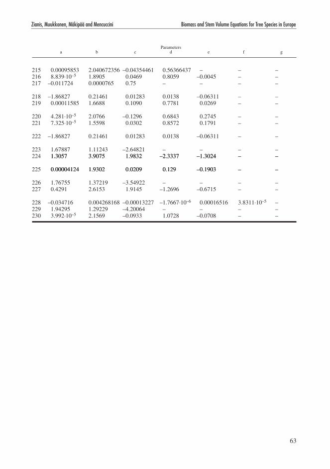
63
Zianis, Muukkonen, Mäkipää and Mencuccini Biomass and Stem Volume Equations for Tree Species in Europe
�15 0.00095853 �.04067�356 –0.04354461 0.56366437 – – –�16 8.839·10–5 1.8905 0.0469 0.8059 –0.0045 – –�17 –0.0117�4 0.0000765 0.75 – – – –
�18 –1.868�7 0.�1461 0.01�83 0.0138 –0.06311 – –�19 0.00011585 1.6688 0.1090 0.7781 0.0�69 – –
��0 4.�81·10–5 �.0766 –0.1�96 0.6843 0.�745 – –��1 7.3�5·10–5 1.5598 0.030� 0.857� 0.1791 – –
��� –1.868�7 0.�1461 0.01�83 0.0138 –0.06311 – –
��3 1.67887 1.11�43 –�.648�1 – – – –��4 1.3057 3.9075 1.983� –�.3337 –1.30�4 – –1.3057 3.9075 1.983� –�.3337 –1.30�4 – –
��5 0.000041�4 1.930� 0.0�09 0.1�9 –0.1903 – –0.000041�4 1.930� 0.0�09 0.1�9 –0.1903 – –
��6 1.76755 1.37�19 –3.549�� – – – –��7 0.4�91 �.6153 1.9145 –1.�696 –0.6715 – –
��8 –0.034716 0.004�68168 –0.00013��7 –1.7667·10–6 0.00016516 3.8311·10–5 –��9 1.94�95 1.�9��9 –4.�0064 – – – –�30 3.99�·10–5 �.1569 –0.0933 1.07�8 –0.0708 – –
Parameters a b c d e f g