bof business international journal of the economics...attendances declined. attendances were...

This article was downloaded by: [University of Liverpool]On: 17 March 2015, At: 03:07Publisher: RoutledgeInforma Ltd Registered in England and Wales Registered Number: 1072954 Registeredoffice: Mortimer House, 37-41 Mortimer Street, London W1T 3JH, UK

Click for updates

International Journal of the Economicsof BusinessPublication details, including instructions for authors andsubscription information:http://www.tandfonline.com/loi/cijb20

Uncertainty of Outcome or StarQuality? Television Audience Demandfor English Premier League FootballBabatunde Buraimoa & Rob Simmonsb

a Management School, University of Liverpool, Chatham Street,Liverpool, L69 7ZH, UKb Management School, Lancaster University, Bailrigg, Lancaster,LA1 4YX, UK,Published online: 16 Mar 2015.

To cite this article: Babatunde Buraimo & Rob Simmons (2015): Uncertainty of Outcome or StarQuality? Television Audience Demand for English Premier League Football, International Journal ofthe Economics of Business, DOI: 10.1080/13571516.2015.1010282

To link to this article: http://dx.doi.org/10.1080/13571516.2015.1010282

PLEASE SCROLL DOWN FOR ARTICLE

Taylor & Francis makes every effort to ensure the accuracy of all the information (the“Content”) contained in the publications on our platform. However, Taylor & Francis,our agents, and our licensors make no representations or warranties whatsoever as tothe accuracy, completeness, or suitability for any purpose of the Content. Any opinionsand views expressed in this publication are the opinions and views of the authors,and are not the views of or endorsed by Taylor & Francis. The accuracy of the Contentshould not be relied upon and should be independently verified with primary sourcesof information. Taylor and Francis shall not be liable for any losses, actions, claims,proceedings, demands, costs, expenses, damages, and other liabilities whatsoever orhowsoever caused arising directly or indirectly in connection with, in relation to or arisingout of the use of the Content.

This article may be used for research, teaching, and private study purposes. Anysubstantial or systematic reproduction, redistribution, reselling, loan, sub-licensing,systematic supply, or distribution in any form to anyone is expressly forbidden. Terms &

http://crossmark.crossref.org/dialog/?doi=10.1080/13571516.2015.1010282&domain=pdf&date_stamp=2015-03-16

http://www.tandfonline.com/loi/cijb20

http://www.tandfonline.com/action/showCitFormats?doi=10.1080/13571516.2015.1010282

http://dx.doi.org/10.1080/13571516.2015.1010282

Conditions of access and use can be found at http://www.tandfonline.com/page/terms-and-conditions

Dow

nloa

ded

by [

Uni

vers

ity o

f L

iver

pool

] at

03:

08 1

7 M

arch

201

5

http://www.tandfonline.com/page/terms-and-conditions

http://www.tandfonline.com/page/terms-and-conditions

Uncertainty of Outcome or Star Quality? Television

Audience Demand for English Premier League

Football

BABATUNDE BURAIMO and ROB SIMMONS

ABSTRACT This paper presents new evidence on the relevance of uncertainty ofoutcome for demand for sports viewing. Using television viewing figures for eightseasons from the English Premier League, we show that uncertainty of outcome doesnot have the hypothesised effect on television audience demand. Separating uncertaintyof outcome effects by season, the results show that, at best, uncertainty of outcome hadimprecise effects on audiences in earlier seasons, but zero effects in later seasons.Television audiences have evolved to exhibit preferences for talent. We suggest that thenotion of a pure sporting contest in which uncertainty of outcome matters is no longerrelevant and more important is the extent to which sports teams and leagues canincrease the quality of the talent on show.

Key Words: Broadcasting; Demand; Uncertainty of Outcome; Soccer; Football;Superstars.

JEL classifications: L82, L83.

1. Introduction

Economic analyses of professional team sports have generally been different tothose of other markets. Unlike conventional markets in which competition isencouraged, economic cooperation is often regarded as a necessary conditionin order to maximise consumer welfare. Neale’s (1964) seminal contributionappraised the peculiar economics of professional sport. Neale noted, amongother things, that monopoly practices were undesirable and there was a needto maintain uncertainty of sporting outcomes. For professional sport to thrive,the presence of viable competitors is desirable so that the unpredictability ofsporting outcomes is maximised. Essentially, the values of sporting contestsare maximised if rivals are evenly matched, as this creates uncertainty ofoutcome.

Babatunde Buraimo, Management School, University of Liverpool, Chatham Street, Liverpool, L69 7ZH,UK; e-mail: [email protected]. Rob Simmons, Management School, Lancaster University, Bailrigg,Lancaster, LA1 4YX, UK; e-mail: [email protected]

� 2015 International Journal of the Economics of Business

Int. J. of the Economics of Business, 2015

http://dx.doi.org/10.1080/13571516.2015.1010282

Dow

nloa

ded

by [

Uni

vers

ity o

f L

iver

pool

] at

03:

08 1

7 M

arch

201

5

mailto:[email protected].

mailto:[email protected]

http://dx.doi.org/10.1080/13571516.2015.1010282

Attempts to maximise uncertainty of outcome in professional sports haveseen the introduction of policies aimed at equalising the playing strengths ofteams organised in leagues. In North American sports, the use of player drafts,salary caps, luxury taxes, and revenue sharing are aimed at maintainingcompetitive balance. In Europe, and more specifically European soccer, similarschemes are not as prevalent, partly due to the overriding principle of freemovement of labour. Players are traded freely, although with some constraintsrelating to work permits for non-EU players. Consequently, talent generallymigrates to big-budget teams where salaries are likely to be at their highest.The only practice that might have an impact on equalising playing strength isthe distribution of broadcast revenue, but policies on this vary across leagues.For example, since the start of the English Premier League in 1992, broadcastrevenues have been systematically shared between its member clubs, whereasclubs negotiate broadcast rights on an individual basis in Spain. Irrespective ofwhether policies to maintain some form of equality between teams actuallyachieve the desired outcome, league authorities have often defended thesepolicies on the grounds of preserving uncertainty of outcome. However, animportant consideration for policymakers is whether preserving uncertainty ofoutcome is actually welfare maximising.

The relevance of uncertainty of outcome needs to be reassessed in the eraof modern professional sports. As a theoretical conjecture that was first putforward in the 1950s (Rottenberg 1956), it has strong merits; the validity of anysporting contest surely depends on the comparative strengths of rivalsinvolved and whether outcomes are predetermined. However, there is a needfor such a conjecture to be empirically validated, particularly if it is going tobe the basis of policymaking and management practice. This is even morerelevant, as there have been numerous changes occurring in professionalsports. Specifically, in the past, the audiences for professional team sports havepredominantly been stadium goers, and they have been the dominant sourceof revenue for leagues and teams. More recently, however, globalisation andadvances in technology have attracted new consumers, and broadcasting isnow a more dominant source of revenue. Many of the world’s leading sports’leagues now generate the majority of their revenue from the sale of rights tobroadcasters who in turn broadcast matches across different platforms andterritories (Cave and Crandall 2001; Solberg 2007). According to Deloitte data,in the 2010–11 season, revenue from broadcasting accounted for 52% of totalrevenue in the English Premier League, 45% in Spain’s Primera Liga, and 60%in Italy’s Serie A. Given the growing importance of broadcasting and televisionaudiences compared with the traditional markets of stadium goers, theconsideration of uncertainty of outcome should not be limited to consumerswho attend sporting contests live at stadia. Television audiences and theirpreferences for outcome uncertainty should be given greater prominence inempirical analysis. Unfortunately, the data needed for this task tend to beelusive.

This paper examines the economic importance of uncertainty of outcomeamong television audiences in the English Premier League. The results showthat the overall impact of uncertainty of outcome on television audiences is notsignificantly different from 0. Separating the impact of uncertainty of outcomeacross different seasons is revealing. The impact of uncertainty of outcome ontelevision audiences in earlier seasons is significant but only at the 10% level.

2 B. Buraimo and R. Simmons

Dow

nloa

ded

by [

Uni

vers

ity o

f L

iver

pool

] at

03:

08 1

7 M

arch

201

5

As the seasons progress from earlier to more recent ones, the impacts ofoutcome uncertainty fall to 0. Rather than valuing contests in which outcomesare uncertain, television audiences now have a preference for matches inwhich the quality of talent (proxied here by the clubs’ wage bills) is high. Thechange in preference from uncertainty of outcome to quality of playing talentcaptures a fundamental shift. “Pure” sporting contests are no longer of valueand have been superseded by entertainment to be delivered by sportssuperstars.

The rest of the article is organised as follows. Section 2 reviews theliterature on the relationship between outcome uncertainty and attendancedemand in sports. Section 3 presents the setting, while Section 4 sets out ourdata set and empirical models. The results are discussed in Section 5, and thefinal section offers concluding remarks.

2. Literature on Uncertainty of Outcome

The extent to which uncertainty of outcome positively impacts consumerdemand and maximises consumer welfare is far from unambiguous(Szymanski 2003). However, the need to preserve it has been defended byleague authorities, and the English Premier League is no exception (RestrictivePractices Court 1999). Many studies have investigated the relationship betweenuncertainty of outcome and demand across a variety of leagues and sports. Forthe most part, these have concentrated on demand for stadium attendance.

Uncertainty of outcome can be viewed at three levels: match level, seasonaldimension, and long run (Borland and Macdonald 2003; Dobson and Goddard2011; Szymanski 2003). The focus of this paper is uncertainty of outcome at thematch level.

In baseball, Knowles, Sherony, and Haupert (1992) examine the effects ofuncertainty of outcome on game-day attendance. Using the probability of ahome win as their measure of uncertainty of outcome and controlling for aseries of factors, they find in favour of the hypothesis that as the home team’s(or the away team’s) probability of winning became more (less) certain,attendances declined. Attendances were maximised when the home team’s winprobability was 0.6, indicating that stadium goers have a preference for ahome win but not dominance. Lee and Fort (2008) and Mills and Fort (2014)similarly examine uncertainty of outcome and attendance in baseball across along period, from 1901. However, they do not find in favour of uncertainty ofoutcome effects at the game level. They do find some evidence in favour ofplay-off uncertainty. Coates, Frick, and Jewell (forthcoming) also studybaseball attendance demand, but their results support ‘loss aversion’ anddirectly contradict the uncertainty of outcome hypothesis. They note that outof 24 attendance demand studies surveyed, only four gave support for theoutcome uncertainty hypothesis. Analyses of uncertainty of outcome in othersports include international cricket (Sacheti, Gregory-Smith, and Paton 2014),rugby (Owen and Weatherston 2004a; 2004b), NBA basketball (Rascher andSolmes 2007), college football (Paul, Humphreys, and Weinbach 2012),American football (Paul, Wachsman, and Weinbach 2011), and soccer(Buraimo, Forrest, and Simmons 2007; Buraimo and Simmons 2008; Czarnitzkiand Stadtmann 2002; Pawlowski 2013).

Uncertainty of Outcome or Star Quality? 3

Dow

nloa

ded

by [

Uni

vers

ity o

f L

iver

pool

] at

03:

08 1

7 M

arch

201

5

There have been a limited number of studies that have modelled televisionaudience demand and even fewer modelling the effects of uncertainty ofoutcome on television demand. Forrest, Simmons, and Buraimo (2005) wereamong the first to examine the effects of uncertainty of outcome amongtelevision audiences and found that uncertainty of outcome did have thetheorised impact on audience demand. Buraimo and Simmons (2009) analyseddemand for both gate attendance and television audiences in Spanish leaguesoccer and found that stadium goers disliked uncertainty of outcome.However, television audiences had a preference for it. Tainsky and McEvoy(2012) also examined the effects of uncertainty of outcome on the size oftelevision audiences in the NFL and found that greater uncertainty resulted ingreater audience demand in line with the hypothesis. Alavy, Gaskell, andSzymanski (2010) used minute-by-minute measures of television audiencedemand in English league football and found in favour of uncertainty ofoutcome. However, the progression of the match and the score line weredominant factors in determining the level of television audiences.

Another strand of literature examines the effects of star quality or brandson audience demand. Studies finding some effects of star quality include Berri,Schmidt, and Brook (2004) on National Basketball Association, and Brandes,Franck, and Nuesch (2008), Czarnitzki and Stadtmann (2002), and Pawlowskiand Anders (2012) all on German Bundesliga. These studies all relate to gateattendance and revenues, and do not consider the effects of star quality onbroadcast audiences, which is our concern in this paper. Previous analyses ofoutcome uncertainty have relied on stadium attendance demand models,partly because television audience data are typically difficult and expensive toobtain. Using a rare television ratings data set from the 2000–01 to 2007–08seasons, we examine the impact of uncertainty of outcome on the size oftelevision audiences.

3. The Setting

The setting for this study is the English Premier League. The English PremierLeague was established in 1992 and currently comprises 20 teams. Theestablishment of the Premier League coincided with advances in technologywhich brought about satellite broadcasting and the entry of pay-televisionoperators. Their emergence saw a dramatic increase in broadcast revenueaccruing to the top tier of English football. Table 1 shows the rights values tothe English Premier League since it started. The increases in broadcastrevenues have made it the most valued soccer league in Europe.

The connection between broadcasting (increase in rights values, revenuesharing among clubs, and number of televised games) and the clubs’motivation to spend large sums in the labour market is an important one (Cox2012). The desire to maximise wins means that clubs are motivated to increasetheir spending in the labour market (see Table 2). The effect of an increase inwage-bill spending by clubs in the league is substantial. The migration ofstar-player talent to the English Premier League makes it a very attractivespectacle to viewers. Broadcasters are willing to invest in this league so as tomaximise television audiences, advertising revenues, and subscriptions whichin turn helps maximise their profits.


Dow

nloa

ded

by [

Uni

vers

ity o

f L

iver

pool

] at

03:

08 1

7 M

arch

201

5

Up until 2003–04, BSkyB, the principal broadcaster, had a monopoly overPremier League broadcasts, and the number of games was limited to 66 perseason. Consequently, consumer demand was restricted to a limited number ofgames. However, the European Commission was unhappy with both themarket structure and the limited outputs (Harbord and Szymanski 2004). In aneffort to keep the Commission and other competition authorities at bay, theleague increased the rights package to four packages with a total of 138games.1 The intention of this restructuring was to allow smaller broadcastersto enter the market. Although more and smaller rights packages wereavailable, BSkyB still acquired the rights to all four packages. BSkyB’smonopoly continued, but consumers now had a greater number of matches toview (88 matches per season). Whilst the net effect was a reduction in themean television audience rating, the total audience across all matchesincreased by 176,000 viewers. This suggests that the previous monopolyarrangements adversely affected consumer welfare. For the 2007–08 season, theEuropean Commission ruled that no single broadcaster should acquire all liverights. It was only then that smaller broadcasters entered the market. Setantawas the first and while its involvement in the market was short-lived (Buraimo2012), the subsequent entries of ESPN and, most recently, British Telecom (BT)represented competition in a market that had been monopolised by BSkyB for15 years. The broadcast rights for the period 2013–14 to 2015–16 generated£3.04 billion for the English Premier League (Hughson 2013). It is this increasein economic significance in the broadcast market for sport which warrants anempirical analysis of the effects of uncertainty of outcome and superstars ontelevision audience demand.

4. Data and Model

Audience data from the 2000–01 to 2007–08 seasons inclusive were obtainedfrom the print versions of the publication TV Sports Markets. The data arelimited to these seasons, and whilst extending the data would be desirable,this is not feasible, since the print version of the publication ceased after 2008.

While the source of data is TV Sports Markets, the origin is the BritishAudience Research Board (BARB), a not-for-profit limited company funded bythe major broadcasters in the UK and the Institute of Practitioners in

Table 1. Rights fees for English Premier League from 1992–93 to 2013–14(Baimbridge, Cameron, and Dawson 1996; Buraimo 2012)

YearDuration of

Contract (years) BroadcastersMatches per

SeasonMean AnnualRights Fee (£m)

Rights Fee perMatch (£m)

1992 5 BSkyB 60 52 0.871997 4 BSkyB 60 199 3.322001 3 BSkyB 66 371 5.622004 3 BSkyB 88 341 3.882007 3 BSkyB and Setanta* 92 and 46 567 4.112010 3 BSkyB and ESPN 115 and 23 594 4.302013 3 BSkyB and BT 116 and 38 1,012 6.58

*Setanta’s administration saw its final season’s rights bought by ESPN.


Dow

nloa

ded

by [

Uni

vers

ity o

f L

iver

pool

] at

03:

08 1

7 M

arch

201

5

Advertising. BARB is the official source for television audience viewing figuresin the UK. Audience sizes derive from more than 30,000 electronic viewingdevices in a sample of more than 5,100 households (http://www.barb.co.uk).These devices measure the number of people watching a programme whenfirst transmitted and also when viewed on playback. The data on viewers arecaptured on a minute-by-minute basis and then averaged across the durationof the programme to generate audience ratings.2 Unlike the Nielsen Ratingsused in the United States which measure the share of the population indesignated market areas, the UK audience ratings are the estimated number ofindividuals watching the programme. Using multistaged, stratified, andunclustered surveys, the viewing figures are then extrapolated for the whole ofthe UK population (http://www.barb.co.uk).

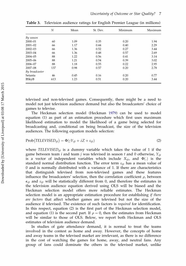
Table 3 provides summary statistics for the television audience ratingsacross the sample period. From the summary data, there was a steady increasein the mean television audience rating from 2000–01 to 2003–04. Since thispeak, per-match audience ratings have declined. The decline coincides with thestructural change in broadcasting regime.

Over the 2000–01 to 2007–08 seasons, a total of 660 out of 3,040 games weretelevised. The effective sample of the audience data set comprises 631 televisedgames. A small number of observations (29 televised games) were droppeddue to missing data. The mean television audience rating was 978,647.3 Notethat the viewing ratings relate to domestic households only and do not includepubs and social clubs where games might be shown.

The television audience rating for a match involving teams i and j in seasont is modelled as follows:

ln AUDIENCEijt

� � ¼ aXijt þ bZþ �ijt (1)

where Xijt is a vector of independent variables and Z is a vector of team,month, and season fixed effects, and �ijt is the disturbance term. A peculiarfeature of the market for televised English Premier League games is that notall games are televised, as the broadcasters have some degree of freedom overmatch selection. If games were modelled using ordinary least squares (OLS),the estimates may be biased if there are differences in the characteristics of

Table 2. English Premier League wage bill and relative wages by season

Season

Wage (in millions of £) Relative Wage (mean = 1)

Mean St. Dev. Minimum Maximum St. Dev. Minimum Maximum

2001–02 35.02 14.87 18.22 62.22 0.426 0.512 1.9442002–03 36.78 15.11 11.37 70.46 0.424 0.303 2.0902003–04 39.38 22.84 19.28 115.57 0.584 0.475 2.8292004–05 38.47 22.28 16.92 108.89 0.573 0.419 2.6952005–06 43.27 26.79 17.35 114.00 0.598 0.383 2.5162006–07 47.36 28.81 17.10 132.82 0.591 0.366 2.7542007–08 59.28 36.70 26.11 171.62 0.652 0.376 2.9742008–09 65.59 36.35 29.75 165.61 0.537 0.448 2.5182009–10 69.96 42.57 22.37 172.55 0.608 0.319 2.479


Dow

nloa

ded

by [

Uni

vers

ity o

f L

iver

pool

] at

03:

08 1

7 M

arch

201

5

http://www.barb.co.uk

http://www.barb.co.uk

televised and non-televised games. Consequently, there might be a need tomodel not just television audience demand but also the broadcasters’ choice ofgames to televise.

The Heckman selection model (Heckman 1979) can be used to modelequation (1) as part of an estimation procedure which first uses maximumlikelihood estimation to model the likelihood of a game being selected forbroadcasting and, conditional on being broadcast, the size of the televisionaudiences. The following equation models selection:

Prob TELEVISEDijt

� � ¼ UðcYijt þ kZþ eijtÞ (2)

where TELEVISEDijt is a dummy variable which takes the value of 1 if thegame between team i and team j was televised in season t and 0 otherwise, Yijt

is a vector of independent variables which include Xijt, and Uð:Þ is thestandard normal distribution function. The error term eijt has a mean value of0 and is normally distributed with a variance of 1. If there are characteristicsthat distinguish televised from non-televised games and these featuresinfluence the broadcasters’ selection, then the correlation coefficient q, between�ijt and eijt will be statistically different from 0, and therefore the estimates inthe television audience equation derived using OLS will be biased and theHeckman selection model offers more reliable estimates. The Heckmanselection model is an appropriate estimation procedure for establishing if thereare factors that affect whether games are televised but not the size of theaudience if televised. The existence of such factors is required for identification.In this respect, equation (2) is the first part of the Heckman selection model,and equation (1) is the second part. If q ¼ 0, then the estimates from Heckmanwill be similar to those of OLS. Below, we report both Heckman and OLSestimates of television audience demand.

In studies of gate attendance demand, it is normal to treat the teamsinvolved in the contest as home and away. However, the concepts of homeand away teams in the televised market are irrelevant, as there is no differencein the cost of watching the games for home, away, and neutral fans. Anygroup of fans could dominate the others in the televised market, unlike

Table 3. Television audience ratings for English Premier League (in millions)

N Mean St. Dev. Minimum Maximum

By season2000–01 60 1.09 0.35 0.20 1.942001–02 66 1.17 0.44 0.40 2.292002–03 66 1.36 0.52 0.27 3.442003–04 66 1.36 0.48 0.57 2.692004–05 88 1.22 0.56 0.41 3.142005–06 88 1.21 0.54 0.39 3.022006–07 88 1.18 0.55 0.22 2.952007–08 137 0.98 0.57 0.20 2.78By broadcasterSetanta 46 0.45 0.16 0.20 0.77BSkyB 613 1.23 0.51 0.20 3.44


Dow

nloa

ded

by [

Uni

vers

ity o

f L

iver

pool

] at

03:

08 1

7 M

arch

201

5

Table 4a. Description of summary statistics

Variable Description

COMBINED RELATIVE WAGE A team’s relative wage is its wage bill for a give seasondivided by the mean wage bill for that season. COMBINEDRELATIVE WAGE is the sum of the two teams’ relativewages.

ABSOLUTE DIFFERENCE INRELATIVE WAGE

This the absolute difference in the two teams’ relative wagebill.

COMBINED LAG POINTS PERGAME

This is the combined points per game from the previousseason of the teams involved in the match.

ABSOLUTE DIFFERENCE IN LAGPOINTS PER GAME

This is the absolute difference in points per game from theprevious season of the teams involved in the match.

COMBINED POINTS PER GAME This is the sum of both teams’ points per game prior to thematch. Points per game is the ratio of the total number ofpoints to the number of games played prior to the match.

ABSOLUTE DIFFERENCE INPOINTS PER GAME

This is the absolute difference in the teams’ points per gameprior to the match. Points per game is the ratio of the totalnumber of points to the number of games played prior to thematch.

CHAMPION CONTENTION This is a dummy variable that takes the value of 1 if either ofthe teams in the match can win the championship if it were towin all its remaining games while others only take an averageof one point from their remaining games and 0 otherwise.

EUROPE CONTENTION This is a dummy variable that takes the value of 1 if either ofthe teams in the match can qualify for either the ChampionsLeague or the Europa Cup but not win the championship if itwere to win all its remaining games while others only take anaverage of one point from their remaining games and 0otherwise.

RELEGATION CONTENTION This is a dummy variable that takes the value of 1 if either ofthe teams in the match can be relegated if it were to win allits remaining games while others only take an average of onepoint from their remaining games and 0 otherwise.

SETANTA This dummy variable is 1 if the match was televised by thebroadcaster Setanta and 0 otherwise. If 0, the match wastelevised by BSkyB.

OTHER MATCHES This is a dummy variable that takes the value of 1 if there areother matches being broadcast at the same time and 0otherwise.

DERBY This is a dummy variable that takes the value of 1 if thematch involves teams who are historical or local rivals and 0otherwise.

WEEKDAY This is a dummy variable that take the value of 1 if the gameis televised on Monday to Friday inclusive and 0 otherwise.

FIRST HALF This is a dummy variable that takes the value of 1 if thematch is played between August and December inclusive and0 otherwise.

SECOND HALF This is a dummy variable that takes the value of 1 if thematch is played between January and May inclusive and 0otherwise.

OUTCOME UNCERTANTY This is the absolute difference in home-win probability andaway-win probability. Probabilities are derived from thebookmaker’s odds and adjusted for over-round.

THEILP3

i¼1 Pi � ln 1pi

� �where Pi is the probability of outcome i

which is any one of the three possible results.


Dow

nloa

ded

by [

Uni

vers

ity o

f L

iver

pool

] at

03:

08 1

7 M

arch

201

5

stadium attendance in which the home team’s fans are always dominant.Instead of home and away, two alternative metrics are used: COMBINED andABSOLUTE DIFFERENCE (see Forrest, Simmons, and Buraimo 2005).

The first of the independent variables in Xijt is COMBINED RELATIVEWAGE. Relative wage is a team’s wage bill for the current season divided bythe mean wage bill for that season. For the eight seasons from 2001–02 to2009–10, the mean wage bill of the English Premier League clubs increasedfrom £35 million to £70 million (Table 2). A typical strategy for many clubs isto improve their playing talent by spending more on better players andinflationary wage-bill increases. Furthermore, the variance in player talent isalso increasing. For example, the standard deviation of wage bill has generallyincreased over the eight seasons shown in Table 2. The use of a relative wage-bill measure normalises the wage bill by the average in a given season. Hence,the mean value of the relative wage bill must be 1. The standard deviationvaries from 0.42 to 0.65, rising over time with the most recent value being 0.61.Hence, the distribution of talent is widening as large clubs outspend others.

Wage-bill data are gathered from various years of Deloitte’s Annual Reviewof Football Finance. The wage-bill data are for all the clubs’ employees and notjust the team. However, it is extremely likely that the wages of the playersdominate those of other employees in the clubs, and it is therefore a goodproxy for the quality of both the squad and the team. Furthermore, the marketmechanism for buying and selling players, which is effectively an auction,means that the best players are also the highest paid. A test of this is thecorrelation between end-of-season performance and wage bill by season. Thecorrelation between performance and wage bill by season is very strong (Hall,Szymanski, and Zimbalist 2002).4 Hence, the wage bill is a good reflection ofskill and quality of talent. As COMBINED RELATIVE WAGE is the sum of thetwo teams’ relative wage and as it increases, it is expected that audience ratingwill also increase as fans have a preference for watching the best talent.ABSOLUTE DIFFERENCE IN RELATIVE WAGE is included to capture thespread of talent across the two teams in the match. With respect to talent, if

Table 4b. Summary statistics for televised games

Variables

Televised games (N = 631)

Mean St. Dev. Minimum Maximum

TELEVISION AUDIENCE RATING 978,647 570,092 204,000 2,780,000COMBINED RELATIVE WAGE 2.368 0.879 0.831 5.067ABSOLUTE DIFFERENCE IN RELATIVE WAGE 0.646 0.559 0.000 2.598COMBINED POINTS PER GAME 3.104 0.815 0 6ABSOLUTE DIFFERENCE IN POINTS PER GAME 0.658 0.525 0 3CHAMPION CONTENTION 0.187 0.390 0 1EUROPE CONTENTION 0.160 0.367 0 1RELEGATION CONTENTION 0.179 0.384 0 1SETANTA 0.071 0.258 0 1OTHER MATCHES 0.025 0.194 0 2DERBY 0.074 0.263 0 1WEEKDAY 0.319 0.466 0 1OUTCOME UNCERTAINTY 0.249 0.180 0 0.712THEIL 1.020 0.095 0.662 1.097


Dow

nloa

ded

by [

Uni

vers

ity o

f L

iver

pool

] at

03:

08 1

7 M

arch

201

5

fans have a preference for a contest in which the quality of talent is evenlydistributed across the teams (Buraimo 2008; Forrest, Simmons, and Buraimo2005), then this variable is in itself a measure of outcome uncertainty. As such,we need to recognise the possibility of multicollinearity with OUTCOMEUNCERTAINTY. Hence, ABSOLUTE DIFFERENCE IN RELATIVE WAGE isincluded in the Heckman selection model, since it represents a prior indicatorof outcome uncertainty before the season starts when the broadcasters begin toselect games.

We use the sum of the two teams’ current points per game up to the matchto derive combined points per game. In English football, three points areawarded for a victory, one point for a draw, and no points for a loss. Themeasure captures the form of the teams prior to the contest. The combinedvalue captures the overall form of the two teams, and higher values are likelyto have a positive impact on audience ratings. The next set of independentvariables captures the extent to which at least one of the teams in the contest isin contention for the championship (winning the league), Europeancompetition the following season, or relegation. Contention is computed usingan algorithm proposed by Goddard and Asimakopoulos (2004). A team is incontention if it wins all its remaining games (three points per game) andothers only tie theirs (one point per game), and in doing so, the team is able towin the title or qualify for Europe. A team is also in contention for relegationif other teams win their remaining matches and it only ties and in doing sowill be relegated. These in contention variables (CHAMPION CONTENTION,EUROPE CONTENTION, and RELEGATION CONTENTION) capture the long-run aspect of competitiveness and are expected to have a positive impact ontelevision audience, ceteris paribus. Previous studies have constructed numerousvariables to capture contention (see, e.g., Jennett 1984; Pawlowski and Anders2012). However, they have all used the number of points necessary to win thechampionship in their measures. The number of points required to win thechampionship is available ex post, and such information is not available toconsumers. It is for this reason that Goddard and Asimakopoulos’s approachis preferred.

Games televised by Setanta in the 2007–08 season feature in the data, and adummy variable, SETANTA, takes the value of 1 if the game was broadcast bythe new entrant. Otherwise, SETANTA take the value of 0, as the game wasbroadcast by BSkyB. Given Setanta’s limited penetration within the televisedfootball market, the coefficient of SETANTA is expected to be negative with alarge magnitude.

Games are televised at different times of the day and week to avoid clashesand cannibalising audience ratings for other games. However, all games on thelast day of the season are played at the same time. A dummy variable, OTHERMATCHES, is included and takes the value of 0 if no other matches areoccurring at the same time and 1 if at least one other match is taking placeconcurrently. Another dummy variable, DERBY, is included to capturematches that involve local and historical rivals. DERBY may or may not besignificant in the context of television audiences. In models of gate attendance,DERBY has proved to be a significant determinant of demand, such is theintense historical and local rivalry between neighbouring football teams(Buraimo 2008; Buraimo, Paramio, and Campos 2010; Forrest and Simmons2006). However, television audiences are drawn from a wider population, and


Dow

nloa

ded

by [

Uni

vers

ity o

f L

iver

pool

] at

03:

08 1

7 M

arch

201

5

such rivalry may be regarded as a local matter. Forrest, Simmons, andBuraimo (2005) found that derby matches had no significant effect ontelevision audiences. Alternatively, national audiences may similarly share thispassion for rivalry.

The final control variable in Xijtis the dummy variable WEEKDAY. Thistakes the value of 0 if the match is televised on Saturday or Sunday and 1otherwise. This is intended to capture the reduced leisure time availableduring the week relative to the abundance of leisure time available at theweekend. As well as these variables, a set of fixed effects is included in Z,comprising team, month, and season effects.

Our focus variable is outcome uncertainty, defined here as the absolutedifference in the two teams’ probability of winning the match. Theprobabilities are derived from the betting odds posted by William Hill, aleading UK bookmaker. The choice of bookmarker is irrelevant, as thecorrelations between posted odds by different bookmakers are extremely high(around 0.95) and the results are robust to the use of different bookmakers’odds. The use of odds to compute probabilities is apt, as they are very strongpredictors of match outcomes, indicating a strong degree of efficiency. Afurther advantage of using betting odds is that they capture all relevant publicas well as private information that is not readily observed but which mayaffect performance, such as player injuries, suspension, and dressing-roommorale.

The sum of unadjusted (home win, away win, and draw) probabilitiesroutinely exceeds unity due to the bookmaker’s margin. This margin, or ‘over-round’, was around 12% over our sample period. The adjusted probabilitiesare derived by dividing each of the probabilities by the sum of unadjustedprobabilities. By doing so, the adjusted values sum to 1. The values ofOUTCOME UNCERTAINTY, the absolute difference in home and away teamprobabilities, for televised games range from 0 to 0.712. A value of 0 representsmatches with the highest degree of uncertainty, while high values representthose matches with a low degree of uncertainty. The values of uncertainty ofoutcome show that there is a high variation, given that the theoretical range isbetween 0 and 1. Hence, there is enough variation to capture any effect ofuncertainty of outcome on audience rating. A shortcoming of this measure isthat the draw probability is assumed constant. This is a reasonableassumption, since there is only a slight variation in the draw probabilitiesacross matches. However, as a robustness check and to deal explicitly with thedraw probability, an alternative measure of outcome uncertainty, the Theilmeasure, is also used (Buraimo and Simmons 2008; Czarnitzki and Stadtmann2002; Peel and Thomas 1992). The Theil measure makes use of the probabilitiesof all three match outcomes and is derived as:

X3i¼1

Pi � ln1

pi

� �

where Pi is the probability of outcome i, which is any one of the three possibleresults. It is highly likely that the results, qualitatively, would be similar, as thecorrelation coefficient between OUTCOME UNCERTAINTY and the Theilmeasure is –0.944.


Dow

nloa

ded

by [

Uni

vers

ity o

f L

iver

pool

] at

03:

08 1

7 M

arch

201

5

Considering the variables in Yijt, selecting games for broadcast is notstraightforward. The challenge that broadcasters face in this market is thatgames selected for broadcast cannot be televised at the regular time of 3:00 pmon Saturday, by League rule. Instead, games must be moved to other times ofthe day (usually noon or 5:30 pm) or other days of the week. The rationale forsuch a move is to reduce the substitution effect that will occur across thewhole of English football, since the majority of football games (in the EnglishPremier League and the three professional divisions of the Football League)take place at 3:00 pm on Saturdays. Many spectators will simply substitutegoing to these games with watching live transmission of Premier Leaguegames. Moving games from 3:00 pm is disruptive, particularly to season-ticketholders who purchase their tickets in advance of the season starting. Tominimise this disruption, a schedule of games for the first half of the season(normally from August to December) is announced prior to the start of theseason. This means that the broadcasters have to choose which games totelevise without any information on how well the teams will be doing. It istherefore likely that the broadcaster will instead make use of other exogenousinformation outside the current season.

Similar to audiences, broadcasters are likely to be attracted to gamesinvolving teams with a high wage bill, a proxy measure for talent. COMBINEDRELATIVE WAGE is likely to have a positive impact on the decision to televisea match. The ABSOLUTE DIFFERENCE IN RELATIVE WAGE is also includedto capture the emphasis that the broadcaster might place on teams who areevenly matched. With respect to talent, broadcasters may have a preference fora contest in which the quality of talent is evenly distributed across the teams(Buraimo 2008; Forrest, Simmons, and Buraimo 2005). The inclusion ofABSOLUTE DIFFERENCE IN RELATIVE WAGE in the selection part of themodel represents a prior indicator of outcome uncertainty before the seasonstarts when the broadcasters begin to select games. To capture the effects ofthe broadcasters’ decision-making process in the first and second half of theseason, COMBINED RELATIVE WAGE and ABSOLUTE DIFFERENCE INRELATIVE WAGE are interacted with FIRST HALF and SECOND HALF. FIRSTHALF takes the value of value 1 for the months between August andDecember and 0 otherwise, and SECOND HALF takes the value of 1 duringthe months January to May and 0 otherwise. By interacting the RELATIVEWAGE variables with FIRST HALF and SECOND HALF, the relative weightsattributed to RELATIVE WAGE during the first and second parts of the seasonby the broadcasters can be evaluated.

Selection for broadcasting is also likely to be based on how popular theteams are. In order to capture the popularity of a given match, the (log of) thecombined mean attendance of the two teams from the previous season, ln(COMBINED LAG ATTENDANCE), is interacted with FIRST HALF to capturethe fact the broadcasters have to select matches for the broadcast schedule forthe first part of the season in advance of the season starting. It is only in thesecond half that they are able to use contemporary information to inform theirselection. In the absence of any information on form, the points at the end ofthe previous season are used as an indicator of future form, at least for thefirst half of the season. Therefore, the combined and the absolute difference inlag points per game, interacted with the dummy variable FIRST HALF, areincluded. During the second half of the season, however, the broadcasters, like


Dow

nloa

ded

by [

Uni

vers

ity o

f L

iver

pool

] at

03:

08 1

7 M

arch

201

5

the television audiences, are able to base their selection decision oncontemporary information. It is with this in mind that COMBINED POINTSPER GAME × SECOND HALF is included. This is the sum of the points pergame of the two teams prior to the current match during the second half of theseason; SECOND HALF is a dummy variable that takes the value of 1 in thesecond half of the season (January to May inclusive) and 0 otherwise.

As with the television audience demand equation, champion contention,Europe contention, and relegation contention are included, but only for thesecond half of the season, since such information is not available to thebroadcasters during the first half of the season. Each of the contentionvariables are therefore interacted with SECOND HALF. The intention of thevariables is to capture any preferences the broadcasters have for gamesinvolving teams in contention of any end-of-season honours over and aboveany uncertainty of outcome. The potential impact of DERBY is also modelled,as this may influence the broadcasters’ selection. The final covariate isOUTCOME UNCERTAINTY. For reasons noted earlier, this is interacted withSECOND HALF. Furthermore, as well as using the absolute difference in homeand away win probabilities, the Theil measure is also used for robustness.Definitions of the variables along with their summary statistics for thetelevised sample are presented in Tables 4a and 4b.

5. Empirical Results

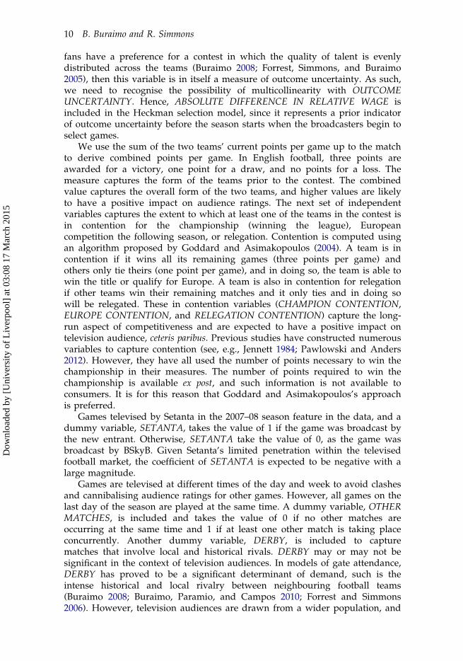
The results of the Heckman selection model with robust standard errorsclustered by rounds5 are presented in Table 5. In the selection part of themodel, the coefficients of COMBINED RELATIVE WAGE × FIRST HALF andCOMBINED RELATIVE WAGE × SECOND HALF are positive, as was to beexpected. However, it is revealing that the coefficient of COMBINEDRELATIVE WAGE × FIRST HALF is greater than that of COMBINEDRELATIVE WAGE × SECOND HALF. In the absence of contemporaryinformation to select games on a round-by-round basis, the wage bills stronglyinfluence the broadcasters’ choice. However, once there is greater freedom ofthe selection, the impact of wage bill falls, although it is still highly significant.This pattern is repeated for ABSOLUTE DIFFERENCE IN RELATIVE WAGE, asthe magnitude of the variable is greater in the second half of the season.Taking the relative wage-bill variables together, the broadcasters’ selection isinfluenced by the total talent and also by how evenly the talent is distributedacross the two teams.

The coefficient of DERBY is significantly different from 0, and broadcastersfavour games with historical and local rivalry attached. The popularity of thegame as measured by ln(COMBINED LAG ATTENDANCE) × FIRST HALF isalso significant, indicating that games involving teams with a strong followingare more likely to be selected for broadcasting in the absence of currentinformation on form. Similarly, games involving teams with high performancesfrom the previous season influence selection in the first part of the season. Itwould also seem that if the previous season’s performances of the two teamsare comparable, this also increases the likelihood of selection given the signand magnitude of the coefficient of ABSOLUTE DIFFERENCE IN LAG POINTSPER GAME × FIRST HALF. The variable COMBINED POINTS PER


Dow

nloa

ded

by [

Uni

vers

ity o

f L

iver

pool

] at

03:

08 1

7 M

arch

201

5

GAME × SECOND HALF has a significant coefficient, and broadcasters valuegames involving high-performing teams. However, such games need notinvolve teams with comparable performance given the insignificant coefficientof ABSOLUTE DIFFENCE IN POINTS PER GAME × SECOND HALF. Of thecontention variables, only EUROPE CONTENTION × SECOND HALF has asignificant coefficient, indicating that as far as end-of-season honours areconcerned, the race for qualifying for European competition stronglyinfluences broadcaster selection of games.

As for the focus variable OUTCOME UNCERTAINTY, its estimated impacton selection is not significantly different from 0. This is a different result tothat shown by Forrest, Simmons, and Buraimo (2005). The evidence suggests

Table 5. Heckman selection model for TV audience ratings

Audience Model: Dependent Variable is ln AUDIENCEijt

� �Coefficient t-Statistic

COMBINED RELATIVE WAGE 0.119** (2.12)ABSOLUTE DIFFERENCE IN RELATIVE WAGE −0.019 (0.51)COMBINED POINTS PER GAME 0.023 (1.25)CHAMPION CONTENTION 0.014 (0.37)EUROPE CONTENTION −0.031 (0.64)RELEGATION CONTENTION −0.019 (0.47)SETANTA −0.966*** (22.94)OTHER MATCHES −0.106 (0.76)DERBY −0.008 (0.19)WEEKDAY −0.083*** (3.85)OUTCOME UNCERTAINTY −0.039 (0.49)CONSTANT 13.037*** (32.44)

Selection model: Dependent variable is Prob TELEVISEDijt

� �Coefficient t-Statistic

COMBINED RELATIVE WAGE × FIRST HALF 0.572*** (7.93)COMBINED RELATIVE WAGE × SECOND HALF 0.275*** (2.84)ABSOLUTE DIFFERENCE IN RELATIVE WAGE × FIRST HALF −0.526*** (5.87)ABSOLUTE DIFFERENCE IN RELATIVE WAGE × SECOND HALF −0.387*** (3.10)DERBY 0.463*** (3.58)LN(COMBINED LAG ATTENDANCE) × FIRST HALF 0.140*** (4.42)COMBINED LAG POINTS PER GAME × FIRST HALF 0.005*** (3.27)ABSOLUTE DIFFERENCE IN LAG POINTS PER GAME × FIRST HALF −0.011*** (3.87)COMBINED POINTS PER GAME × SECOND HALF 0.782*** (6.81)ABSOLUTE DIFFERENCE IN POINTS PER GAME × SECOND HALF 0.175 (0.99)CHAMPION CONTENTION × SECOND HALF 0.141 (1.28)EUROPE CONTENTION × SECOND HALF 0.272*** (3.09)RELEGATION CONTENTION × SECOND HALF −0.006 (0.06)OUTCOME UNCERTAINTY × SECOND HALF 0.059 (0.19)CONSTANT −3.647*** (13.65)Lambda 0.007 0.083Rho 0.026Observations 2872

Absolute t-statistics in parentheses. Clustered by round of match using robust standard errors.*p < 0.10**p < 0.05.***p < 0.01. Month, season, and team effects are significant.


Dow

nloa

ded

by [

Uni

vers

ity o

f L

iver

pool

] at

03:

08 1

7 M

arch

201

5

that broadcasters’ selection is no longer driven by uncertainty of outcome andother factors are more important in the selection choice.

For the second part of the Heckman model, audience, the only variableswhich have statistically significant coefficients are COMBINED RELATIVEWAGE, WEEKDAY, and SETANTA. The relevance of SETANTA in this contextis to suggest that the platform on which the game is transmitted matters. Thisis not surprising given that different platforms have different levels ofpenetration in the football broadcast market. As for WEEKDAY, the significantcoefficient signals that, due to relative lack of leisure time during the week,games televised from Monday to Friday inclusive have lower audiencescompared with those televised at the weekend, a marginal negative effect of8.3%. Therefore, controlling for broadcast market conditions and teamidiosyncrasies, COMBINED RELATIVE WAGE is all that matters to televisionaudiences. Unlike the broadcasters who care how the talent is distributedacross the two teams, television audiences are indifferent to this, and all thatmatters is that the volume of talent on display is high, whichever team hasthat talent. The fixed effects for months, seasons, and teams are included, andeach set is significant. Hence, the impacts of talent noted are over and abovethe effects of specific teams which in themselves influence the size of televisionaudiences that tune in.

The use of the Heckman sample selection correction reveals that thecorrelation between the error terms from the selection and demand equationsis not significantly different from 0. This indicates that there are no discerningfeatures between those matches that are broadcast and those that are not. Theeffect of this result is that the estimates from the demand equation are notsignificantly different from those that would otherwise be derived from OLS,that is, there is no selection bias.

As well as using a Heckman selection model, OLS is used to model TVaudiences. The results of the OLS estimates are shown in Table 6. We test forthe normality of the residuals in each of the models noted in Table 6. The testsshow that the hypothesis that the residuals are normally distributed with a 0mean cannot be rejected. In model 1 of Table 6, and also the Heckman model,the variables with significant coefficients are COMBINED RELATIVE WAGE,WEEKDAY, and SETANTA. Irrespective of model specification, the OUTCOMEUNCERTAINTY variable has a coefficient that is not significantly differentfrom 0. The significance of the COMBINED RELATIVE WAGE coefficientindicates that audience size is influenced by the total quality of players acrossthe two teams; the higher the COMBINED RELATIVE WAGE, the greater theaudience rating. The magnitude of the effect is such that if the quality ofplayers as represented by relative wage bill were to improve by one standarddeviation, the audience size is estimated to increase by 11.1%, an increase ofapproximately 108,389 viewers per match on BSkyB’s platform. Given thatdeviations in recent season have increased, if the standard deviation ofCOMBINED RELATIVE WAGE for televised games in the most recent season(0.924) were to be used, the increase in television audience is 113,938 viewersper match. These increases are non-trivial given that this is a subscriptionplatform. It is therefore in the broadcasters’ interest to televise those games inwhich the available talent on show is high.

ABSOLUTE DIFFERENCE IN RELATIVE WAGE and ABSOLUTEDIFFERENCE IN POINTS PER GAME had insignificant coefficients and were


Dow

nloa

ded

by [

Uni

vers

ity o

f L

iver

pool

] at

03:

08 1

7 M

arch

201

5

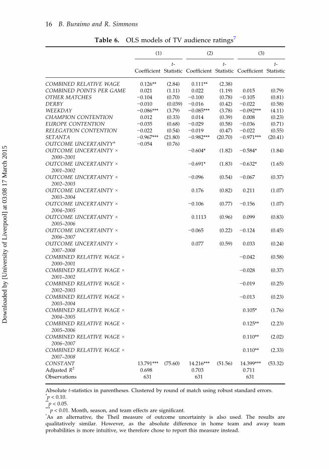
Table 6. OLS models of TV audience ratings7

(1) (2) (3)

Coefficientt-

Statistic Coefficientt-

Statistic Coefficientt-

Statistic

COMBINED RELATIVE WAGE 0.126** (2.84) 0.111** (2.38)COMBINED POINTS PER GAME 0.021 (1.11) 0.022 (1.19) 0.015 (0.79)OTHER MATCHES −0.104 (0.70) −0.100 (0.78) −0.105 (0.81)DERBY −0.010 (0.039) −0.016 (0.42) −0.022 (0.58)WEEKDAY −0.086*** (3.79) −0.085*** (3.78) −0.092*** (4.11)CHAMPION CONTENTION 0.012 (0.33) 0.014 (0.39) 0.008 (0.23)EUROPE CONTENTION −0.035 (0.68) −0.029 (0.58) −0.036 (0.71)RELEGATION CONTENTION −0.022 (0.54) −0.019 (0.47) −0.022 (0.55)SETANTA −0.967*** (21.80) −0.982*** (20.70) −0.971*** (20.41)OUTCOME UNCERTAINTYa −0.054 (0.76)OUTCOME UNCERTAINTY ×

2000–2001−0.604* (1.82) −0.584* (1.84)

OUTCOME UNCERTAINTY ×2001–2002

−0.691* (1.83) −0.632* (1.65)


−0.096 (0.54) −0.067 (0.37)


0.176 (0.82) 0.211 (1.07)


−0.106 (0.77) −0.156 (1.07)


0.1113 (0.96) 0.099 (0.83)


−0.065 (0.22) −0.124 (0.45)


0.077 (0.59) 0.033 (0.24)

COMBINED RELATIVE WAGE ×2000–2001

−0.042 (0.58)


−0.028 (0.37)


−0.019 (0.25)


−0.013 (0.23)


0.105* (1.76)


0.125** (2.23)


0.110** (2.02)


0.110** (2.33)

CONSTANT 13.791*** (75.60) 14.216*** (51.56) 14.399*** (53.32)Adjusted R2 0.698 0.703 0.711Observations 631 631 631

Absolute t-statistics in parentheses. Clustered by round of match using robust standard errors.*p < 0.10.**p < 0.05.***p < 0.01. Month, season, and team effects are significant.a

As an alternative, the Theil measure of outcome uncertainty is also used. The results arequalitatively similar. However, as the absolute difference in home team and away teamprobabilities is more intuitive, we therefore chose to report this measure instead.


Dow

nloa

ded

by [

Uni

vers

ity o

f L

iver

pool

] at

03:

08 1

7 M

arch

201

5

duly dropped from the regression. Their exclusion can be justified on thegrounds of collinearity with OUTCOME UNCERTAINTY. The effect ofCOMBINED POINTS PER GAME is not significantly different from 0.Television audiences are influenced more so by the identity of the teams andnot their respective performances to date. The dummy variables OTHERMATCHES and DERBY and the CONTENTION variables do not havesignificant impacts on the size of television audiences. The dummy variableOTHER MATCHES is intended to capture the greater proportion of gamestelevised on the last day of the season, but the lack of significance wouldsuggest that such games are not substitutes for one another. This raises theinteresting prospect that it might be possible for broadcasters to televise gamesconcurrently without harming total audience ratings. This is particularlyrelevant, as the number of live games from one contract period to the next hasincreased, but as the number of games increases, it might be necessary totelevise some matches concurrently. For DERBY matches, it would seem thatthe attraction of such games is limited, ceteris paribus, to stadium goers and nottelevision viewers.

Audience ratings for matches televised during the week are lowercompared with those televised at the weekend; the fall in audience rating is ofthe magnitude of 8.6%. This is likely to be capturing the limited amount ofleisure time available to audiences during the week compared with theweekend. Also, those games televised by Setanta attracted far fewer audiencescompared to those televised on BSkyB’s channels. During the period ofanalysis, Setanta’s penetration within UK households was much smallercompared with BSkyB’s.

The coefficient of the focus variable OUTCOME UNCERTAINTY is notsignificantly different from 0, and this result is robust to a series of modellingapproaches.6 This finding is contrary to those reported in earlier papers(Buraimo and Simmons 2009; Forrest, Simmons, and Buraimo 2005) and couldbe capturing an evolution in television audiences’ preferences. We interact thefocus variable with season dummy variables. The estimates are reported inmodel 2 of Table 6. The coefficients of OUTCOME UNCERTAINTY interactedwith 2000–2001 and 2001–2002 are significantly different from 0 (at the 10%level) with the appropriate signs showing, tentatively, that television audiencesvalue contests that are close. However, in the seasons after 2002, thecoefficients of OUTCOME UNCERTAINTY interacted with each season from2003–2003 to 2007–2008 are not significantly different from 0. This would seemto mark a transition away from valuing uncertainty of outcome. To exploretelevision audience demand further, COMBINED RELATIVE WAGE is alsointeracted with seasons, and the results are shown in model 3 of Table 6.Strikingly, the interaction of COMBINED RELATIVE WAGE with the earliestfour seasons is not significantly different from 0. However, for the seasons2004–05 to 2007–08 inclusive, COMBINED RELATIVE WAGE interacted withseason has significant coefficients. Again, it should be noted that these impactsare over and above the team fixed effects which already distinguish betweenthe identity and brand of the teams. For example, the reported effect ofCOMBINED RELATIVE WAGE is in addition to the effects of individual teamswhich would attract large audiences anyway.

This is a major result that policymakers and league authorities should notignore. The central finding of this paper suggests that consumer interest has


Dow

nloa

ded

by [

Uni

vers

ity o

f L

iver

pool

] at

03:

08 1

7 M

arch

201

5

shifted away from uncertainty of outcome to the quality of playing talent.Television audiences are drawn to games with a greater presence of star talenton show. Preferences for balanced contests and the anticipation of an uncertainoutcome appear to have waned amongst television audiences. Instead, decisionmakers and league authorities should concern themselves with one dominantstrategy: maximising the quality of talent coming into the league. For this tohappen, clubs will need to continue to spend large sums of money onrecruiting talent. Assessment of efforts to control such costs at the levels ofleague and governing body are beyond the scope of this paper (see, e.g.,Franck [2014] and Peeters and Szymanski [2014] on UEFA’s Financial Fair Playpolicy), but such efforts need to be reconciled with the preferences of viewersas expressed through audience demand.

Acquisition of star players to satisfy viewer preferences implies a netmigration of talent into the league. However, such migration must be at theexpense of other leagues. The league and its clubs therefore have an incentiveto attract the best players to the league. They must be able to meet the cost ofsuch extravagance, and one major source of finance is the revenues from thetelevision broadcast sector. In the case of the English Premier League, it isimperative that it maximises the revenue that it generates from the broadcastmarket. Consequently, its rights strategy must give considerable attention tohow to make use of the growing competition amongst broadcasters,particularly if it is to attract talent which in turn will maximise audiencedemand.

6. Concluding Remarks

This paper examines the notion that uncertainty of outcome matters to footballaudiences and, more specifically, television audiences for the English PremierLeague. The concept of uncertainty of outcome is a central conjecture in theeconomics literature on professional team sports, and since it was firstpresented, its relevance to policymaking and management practices inprofessional sports leagues has been strong. The empirical testing ground foruncertainty of outcome has usually been stadium attendees. Traditionally,income from stadia has been the dominant source of revenue. However, intoday’s sports markets in which the supply of talent to sports leagues is global,attention should shift to television audiences for sport. The use of televisionaudiences over stadium attendees to test the uncertainty of outcomehypothesis is more appropriate.

We find that uncertainty of outcome does not have a significant impact ontelevision audience ratings overall. Separating the measure of uncertainty ofoutcome by seasons shows significant coefficients over the first two seasons ofour sample, albeit at the 10% level. But over seasons, this significancedisappears. The dissipation of the uncertainty of outcome effect coincides withan increase in the quality of talent employed in the English Premier League.We argue that there has been a transition of preference for uncertainty ofoutcome towards a preference for increased talent. The classic notion of a puresporting contest in which the outcome is unpredictable has been replaced withone in which the preference is for sporting entertainment delivered bysuperstars. The unpredictability of the outcome no longer matters for television


Dow

nloa

ded

by [

Uni

vers

ity o

f L

iver

pool

] at

03:

08 1

7 M

arch

201

5

viewers. The implications of these findings are that leagues should no longerdefend their practices on the ground of uncertainty of outcome, andconsequently the defence of sports policies should be reconsidered.Furthermore, if consumer welfare is to be maximised, maximising uncertaintyof outcome is unlikely to achieve this. Instead, policies and strategies aimed atthe labour market and how it operates should be the focus of leagueadministrators. The policy recommendation that emerges from this analysis isthat the league (and its constituent clubs) needs to increase the quality oftalent migrating into the league; the distribution of such talent across the clubsis presently of little significance. Attempts to increase the quality of talentcoming into the league mean direct competition against other leaguescompeting for the same talent. The league should create the right incentivesfor clubs to attract the best players, and similarly clubs need to create the righteconomic incentives to attract players from other leagues. This in turn willmaximise television audience ratings.

Notes

1. Interestingly, in the German Bundesliga, there is a single broadcaster (Sky), and all games aretelevised. This suggests some variation in policies towards football broadcasting across the EU.

2. Whilst minute-by-minute data would be more insightful in measuring television audiencedemand, such data are not readily available. As noted above, only one study (Alavy, AlisonGaskell, and Szymanski 2010) has made use of minute-by-minute measures of audience ratings.

3. The mean gate attendance over this period was 34,474 per match (from Sky Sports FootballYearbook).

4. In the 2000–01 season, the correlation coefficient between performance and wages was 0.675. Bythe 2007–08 season, this had risen to 0.814. The mean correlation coefficient across the eightseasons is 0.795. In recent seasons, this figure has reached 0.888.

5. The standard errors are clustered by the rounds of matches, as the choice of matches to betelevised is constrained by the fixture list. For a given set of matches in a given round, thebroadcasters must select a proportion of matches for that given weekend. This is a significantconstraint, as the broadcasters cannot select the best n matches from 380 games. In this sense,the round of the fixture list is binding, and a proportion of games from those available thatweekend must be chosen. This is the condition for which the models are clustered. The standarderrors of the models are therefore adjusted to reflect this.

6. We also use instrumental variable regression in which we treat OUTCOME UNCERTAINTY asendogenous. In doing so, the variables Absolute difference in relative wage and Absolute difference inpoints per game are used as instruments. The results were similar to those generated using OLS.

7. The Ramsey reset test is used to test the functional form of the models. The results of the testindicate that the models are correctly specified. Furthermore, the null hypothesis that themodels have no omitted variables cannot be rejected. With respect to multicollinearity, varianceinflation factor is used. The results indicate that multicollinearity does not affect the coefficients.

References

Alavy, Kevin, Alison Gaskell, Stephanie Leach, and Stefan Szymanski. 2010. On the Edge of YourSeat: Demand for Football on Television and the Uncertainty of Outcome Hypothesis.International Journal of Sport Finance 5 (2): 75–95.

Baimbridge, Mark, Samuel Cameron, and Peter Dawson. 1996. Satellite Television and the Demandfor Football: A Whole New Ball Game? Scottish Journal of Political Economy 43 (3): 317–333.

Berri, David, Martin Schmidt, and Stacey Brook. 2004. Stars at the Gate: The Impact of Star Poweron NBA Gate Revenues. Journal of Sports Economics 5 (1): 33–50.

Borland, Jeffery, and Robert MacDonald. 2003. Demand for Sport. Oxford Review of Economic Policy19 (4): 478–502.


Dow

nloa

ded

by [

Uni

vers

ity o

f L

iver

pool

] at

03:

08 1

7 M

arch

201

5

Brandes, Leif, Egon Franck, and Stephan Nuesch. 2008. Local Heroes and Superstars: An EmpiricalAnalysis of Star Attraction in German Soccer. Journal of Sports Economics 9 (3): 266–286.

Buraimo, Babatunde. 2008. Stadium Attendance and Television Audience Demand in EnglishLeague Football. Managerial and Decision Economics 29 (6): 513–523.

Buraimo, Babatunde. 2012. Attendance and Broadcast Demand for Professional Team Sports: TheCase of English League Football. In Routledge Handbook of Sport Management, edited by LeighRobinson, Guillaume Bodet, Packianathan Chelladurai, and Paul Downward, 405–418. Oxon:Routledge.

Buraimo, Babatunde, David Forrest, and Rob Simmons. 2007. Outcome Uncertainty Measures: HowClosely Do They Predict a Close Game? In Statistical Thinking in Sports, edited by Jim Albert andRuud Koning, 167–178. London: Chapman & Hall/CRC.

Buraimo, Babatunde, Juan Luis Paramio, and Carlos Campos. 2010. The Impact of TelevisedFootball on Stadium Attendances in English and Spanish League Football. Soccer & Society 11 (4):461–474.

Buraimo, Babatunde, and Rob Simmons. 2008. Do Sports Fans Really Value Uncertainty ofOutcome: Evidence from the English Premier League. International Journal of Sport Finance 3 (3):146–155.

Buraimo, Babatunde, and Rob Simmons. 2009. A Tale of Two Audiences: Spectators, TelevisionViewers and Outcome Uncertainty in Spanish Football. Journal of Economics and Business 61 (4):326–338.

Cave, Martin, and Robert W. Crandall. 2001. Sports Rights and the Broadcasting Industry. EconomicJournal 111: 4–26.

Coates, Dennis, Bernd Frick, and Todd Jewell. forthcoming. Superstar Salaries and Soccer Successthe Impact of Designated Players in Major League Soccer. Journal of Sports Economics.

Cox, Adam. 2012. Live Broadcasting. Gate Revenue, and Football Club Performance: SomeEvidence, International Journal of the Economics of Business 19 (1): 75–98.

Czarnitzki, Dirk, and Georg Stadtmann. 2002. Uncertainty of Outcome versus Reputation:Empricial Evidence for the First German Football Division. Empirical Economics 27 (1): 101–112.

Dobson, Stephen, and John Goddard. 2011. The Economics of Football. 2nd ed. Cambridge:Cambridge University Press.

Forrest, David, and Rob Simmons. 2006. New Issues in Attendance Demand the Case of theEnglish Football League. Journal of Sports Economics 7 (3): 247–266.

Forrest, David, Robert Simmons, and Babatunde Buraimo. 2005. Outcome Uncertainty and theCouch Potato Audience. Scottish Journal of Political Economy 52 (4): 641–661.

Franck, Egon. 2014. Financial Fair Play in European Club Football: What is It All about?International Journal of Sport Finance 9 (3): 193–217.

Goddard, John, and Ioannis Asimakopoulos. 2004. Forecasting Football Results and the Efficiencyof Fixed-Odds Betting. Journal of Forecasting 23: 51–66.

Hall, Stephen, Stefan Szymanski, and Andrew S. Zimbalist. 2002. Testing Causality between TeamPerformance and Payroll the Cases of Major League Baseball and English Soccer. Journal of SportsEconomics 3 (2): 149–168.

Harbord, David, and Stefan Szymanski. 2004. Football Trials. European Competition Law Review 25(2): 117–121.

Heckman, James J. 1979. Sample Selection Bias as a Specification Error. Econometrica 47 (1): 153–161.Hughson, John. 2013. Watching the Football with Raymond Wiliams: A Reconsideration of theGlobal Game as a Wonderful Game. In Sport, Public Broadcasting, and Cultural Citizenship: SignalLost?, edited by Scherer, Jay and David Rowe, 283–299. Oxon: Routledge.

Jennett, Nicholas. 1984. Attendances, Uncertainty of Outcome and Policy in Scottish LeagueFootball. Scottish Journal of Political Economy 31 (2): 176–198.

Knowles, Glenn, Keith Sherony, and Mike Haupert. 1992. The Demand for Major League Baseball:A Test of the Uncertainty of Outcome Hypothesis. The American Economist 36 (2): 72–80.

Lee, Young Hoon, and Rodney Fort. 2008. Attendance and the Uncertainty-of-Outcome Hypothesisin Baseball. Review of Industrial Organization 33 (4): 281–295.

Mills, Brian, and Rodney Fort. 2014. League-Level Attendance and Outcome Uncertainty in US proSports Leagues. Economic Inquiry 52 (1): 205–218.

Neale, Walter C. 1964. The Peculiar Economics of Professional Sports. Quarterly Journal of Economics78 (1): 1–14.


Dow

nloa

ded

by [

Uni

vers

ity o

f L

iver

pool

] at

03:

08 1

7 M

arch

201

5

Owen, P. Dorian, and Clayton R. Weatherston. 2004a. Uncertainty of Outcome and Super 12 RugbyUnion Attendance Application of a General-to-Specific Modeling Strategy. Journal of SportsEconomics 5 (4): 347–370.

Owen, P. Dorian, and Clayton R. Weatherston. 2004b. Uncertainty of Outcome, Player Quality andAttendance at National Provincial Championship Rugby Union Matches: An Evaluation in Lightof the Competitions Review. Economic Papers: A Journal of Applied Economics and Policy 23 (4):301–324.

Paul, Rodney, Brad R. Humphreys, and Andrew Weinbach. 2012. Uncertainty of Outcome andAttendance in College Football: Evidence from Four Conferences. Economic and Labour RelationsReview 23 (2): 69–82.

Paul, Rodney J., Yoav Wachsman, and Andrew P. Weinbach. 2011. The Role of Uncertainty ofOutcome and Scoring in the Determination of Fan Satisfaction in the NFL. Journal of SportsEconomics 12 (2): 213–221.

Pawlowski, Tim. 2013. Testing the Uncertainty of Outcome Hypothesis in European ProfessionalFootball: A Stated Preference Approach. Journal of Sports Economics 14 (4): 341–367.

Pawlowski, Tim, and Christoph Anders. 2012. Stadum Attendance in German ProfessionalFootball- the (Un)Importance of Uncertainty of Outcome Revisited. Applied Economics Letters 19(16): 1553–1556.

Peel, David, and Dennis Thomas. 1992. The Demand for Football: Some Evidence on OutcomeUncertainty. Empirical Economics 17 (2): 323–331.

Peeters, Thomas, and Stefan Szymanski. 2014. Financial Fair Play in European Football. EconomicPolicy 29 (78): 343–390.

Rascher, Daniel A., and John Paul G. Solmes. 2007. Do Fans Want Close Contests? A Test of theUncertainty of Outcome Hypothesis in the National Basketball Association. International Journal ofSport Finance 2 (3): 130–141.

Restrictive Practices Court. 28 July, 1999. Premier League Judgement, E&W No. 1.Rottenberg, Simon. 1956. The Baseball Players’ Labor Market. Journal of Political Economy 64:242–258.

Sacheti, Abhinav, Ian Gregory-Smith, and David Paton. 2014. Uncertainty of Outcome or Strengthsof Teams: An Economic Analysis of Attendance Demand for International Cricket. AppliedEconomics 46 (17): 2034–2046.

Solberg, Harry Arne. 2007. The Auctioning of TV-Sports Rights. International Journal of Sport Finance1 (1): 33–45.

Szymanski, Stefan. 2003. The Economic Design of Sporting Contest. Journal of Economic Literature 41(4): 1137–1187.

Tainsky, Scott, and Chad D. McEvoy. 2012. Television Broadcast Demand in Markets without LocalTeams. Journal of Sports Economics 13 (3): 250–265.


Dow

nloa

ded

by [

Uni

vers

ity o

f L

iver

pool

] at

03:

08 1

7 M

arch

201

5

bof business international journal of the economics...attendances declined. attendances were...

Documents