book2 v free
TRANSCRIPT
Fourier and Wavelet Signal Processing
Jelena Kovacevic
Carnegie Mellon University
Vivek K Goyal
Massachusetts Institute of Technology
Martin Vetterli
Ecole Polytechnique Federale de Lausanne
January 17, 2013
Copyright (c) 2013 Jelena Kovacevic, Vivek K Goyal, and Martin Vetterli.These materials are protected by copyright under the
Attribution-NonCommercial-NoDerivs 3.0 Unported Licensefrom Creative Commons.
Contents
Image Attribution ix
Quick Reference xi
Preface xvii
Acknowledgments xxi
1 Filter Banks: Building Blocks of Time-Frequency Expansions 1
1.1 Introduction 21.2 Orthogonal Two-Channel Filter Banks 7
1.2.1 A Single Channel and Its Properties 71.2.2 Complementary Channels and Their Properties 101.2.3 Orthogonal Two-Channel Filter Bank 111.2.4 Polyphase View of Orthogonal Filter Banks 141.2.5 Polynomial Approximation by Filter Banks 18
1.3 Design of Orthogonal Two-Channel Filter Banks 201.3.1 Lowpass Approximation Design 201.3.2 Polynomial Approximation Design 211.3.3 Lattice Factorization Design 25
1.4 Biorthogonal Two-Channel Filter Banks 261.4.1 A Single Channel and Its Properties 291.4.2 Complementary Channels and Their Properties 321.4.3 Biorthogonal Two-Channel Filter Bank 321.4.4 Polyphase View of Biorthogonal Filter Banks 341.4.5 Linear-Phase Two-Channel Filter Banks 35
1.5 Design of Biorthogonal Two-Channel Filter Banks 371.5.1 Factorization Design 371.5.2 Complementary Filter Design 391.5.3 Lifting Design 40
1.6 Two-Channel Filter Banks with Stochastic Inputs 411.7 Computational Aspects 42
1.7.1 Two-Channel Filter Banks 421.7.2 Boundary Extensions 46
Chapter at a Glance 49Historical Remarks 52Further Reading 52
2 Local Fourier Bases on Sequences 55
2.1 Introduction 562.2 N -Channel Filter Banks 59
2.2.1 Orthogonal N -Channel Filter Banks 592.2.2 Polyphase View of N -Channel Filter Banks 61
2.3 Complex Exponential-Modulated Local Fourier Bases 662.3.1 Balian-Low Theorem 672.3.2 Application to Power Spectral Density Estimation 682.3.3 Application to Communications 73
2.4 Cosine-Modulated Local Fourier Bases 752.4.1 Lapped Orthogonal Transforms 762.4.2 Application to Audio Compression 83
2.5 Computational Aspects 85Chapter at a Glance 87Historical Remarks 88Further Reading 90
3 Wavelet Bases on Sequences 91
3.1 Introduction 933.2 Tree-Structured Filter Banks 99
3.2.1 The Lowpass Channel and Its Properties 993.2.2 Bandpass Channels and Their Properties 1033.2.3 Relationship between Lowpass and Bandpass Channels105
3.3 Orthogonal Discrete Wavelet Transform 1063.3.1 Definition of the Orthogonal DWT 1063.3.2 Properties of the Orthogonal DWT 107
3.4 Biorthogonal Discrete Wavelet Transform 1123.4.1 Definition of the Biorthogonal DWT 1123.4.2 Properties of the Biorthogonal DWT 114
3.5 Wavelet Packets 1143.5.1 Definition of the Wavelet Packets 1153.5.2 Properties of the Wavelet Packets 116
3.6 Computational Aspects 116Chapter at a Glance 118Historical Remarks 119Further Reading 119
4 Local Fourier and Wavelet Frames on Sequences 121
4.1 Introduction 1224.2 Finite-Dimensional Frames 133
4.2.1 Tight Frames for CN 1334.2.2 General Frames for CN 140
4.2.3 Choosing the Expansion Coefficients 1454.3 Oversampled Filter Banks 151
4.3.1 Tight Oversampled Filter Banks 1524.3.2 Polyphase View of Oversampled Filter Banks 155
4.4 Local Fourier Frames 1584.4.1 Complex Exponential-Modulated Local Fourier Frames1594.4.2 Cosine-Modulated Local Fourier Frames 163
4.5 Wavelet Frames 1654.5.1 Oversampled DWT 1654.5.2 Pyramid Frames 1674.5.3 Shift-Invariant DWT 170
4.6 Computational Aspects 1714.6.1 The Algorithm a Trous 1714.6.2 Efficient Gabor and Spectrum Computation 1714.6.3 Efficient Sparse Frame Expansions 171
Chapter at a Glance 173Historical Remarks 174Further Reading 174
5 Local Fourier Transforms, Frames and Bases on Functions 177
5.1 Introduction 1785.2 Local Fourier Transform 178
5.2.1 Definition of the Local Fourier Transform 1785.2.2 Properties of the Local Fourier Transform 182
5.3 Local Fourier Frame Series 1885.3.1 Sampling Grids 1885.3.2 Frames from Sampled Local Fourier Transform 188
5.4 Local Fourier Series 1885.4.1 Complex Exponential-Modulated Local Fourier Bases 1885.4.2 Cosine-Modulated Local Fourier Bases 188
5.5 Computational Aspects 1885.5.1 Complex Exponential-Modulated Local Fourier Bases 1885.5.2 Cosine-Modulated Local Fourier Bases 188
Chapter at a Glance 188Historical Remarks 188Further Reading 188
6 Wavelet Bases, Frames and Transforms on Functions 189
6.1 Introduction 1896.1.1 Scaling Function and Wavelets from Haar Filter Bank1906.1.2 Haar Wavelet Series 1956.1.3 Haar Frame Series 2026.1.4 Haar Continuous Wavelet Transform 204
6.2 Scaling Function and Wavelets from Orthogonal Filter Banks 2086.2.1 Iterated Filters 2086.2.2 Scaling Function and its Properties 209
6.2.3 Wavelet Function and its Properties 2186.2.4 Scaling Function and Wavelets from Biorthogonal
Filter Banks 2206.3 Wavelet Series 222
6.3.1 Definition of the Wavelet Series 2236.3.2 Properties of the Wavelet Series 2276.3.3 Multiresolution Analysis 2306.3.4 Biorthogonal Wavelet Series 239
6.4 Wavelet Frame Series 2426.4.1 Definition of the Wavelet Frame Series 2426.4.2 Frames from Sampled Wavelet Series 242
6.5 Continuous Wavelet Transform 2426.5.1 Definition of the Continuous Wavelet Transform 2426.5.2 Existence and Convergence of the ContinuousWavelet
Transform 2436.5.3 Properties of the Continuous Wavelet Transform 244
6.6 Computational Aspects 2546.6.1 Wavelet Series: Mallat’s Algorithm 2546.6.2 Wavelet Frames 259
Chapter at a Glance 259Historical Remarks 259Further Reading 259
Bibliography 265

Quick Reference
Abbreviations
AR AutoregressiveARMA Autoregressive moving averageAWGN Additive white Gaussian noiseBIBO Bounded input, bounded outputCDF Cumulative distribution functionDCT Discrete cosine transformDFT Discrete Fourier transformDTFT Discrete-time Fourier transformDWT Discrete wavelet transformFFT Fast Fourier transformFIR Finite impulse responsei.i.d. Independent and identically distributedIIR Infinite impulse responseKLT Karhunen–Loeve transformLOT Lapped orthogonal transformLPSV Linear periodically shift varyingLSI Linear shift invariantMA Moving averageMSE Mean square errorPDF Probability density functionPOCS Projection onto convex setsROC Region of convergenceSVD Singular value decompositionWSCS Wide-sense cyclostationaryWSS Wide-sense stationary
Abbreviations used in tables and captions but not in the text
FT Fourier transformFS Fourier seriesLFT Local Fourier transformWT Wavelet transform

Elements of Setsnatural numbers N 0, 1, . . .integers Z . . . , −1, 0, 1, . . .positive integers Z
+ 1, 2, . . .real numbers R (−∞,∞)
positive real numbers R+ (0,∞)
complex numbers C a+ jb or rejθ with a, b, r, θ ∈ R
a generic index set Ia generic vector space Va generic Hilbert space H
real part of ℜ( · )imaginary part of ℑ( · )closure of set S S
functions x(t) argument t is continuous valued, t ∈ R
sequences xn argument n is an integer, n ∈ Z
ordered sequence (xn)nset containing xn xnnvector x with xn as elements [xn]
Dirac delta function δ(t)
∫ ∞
−∞x(t)δ(t)dt = x(0)
Kronecker delta sequence δn δn = 1 for n = 0; δn = 0 otherwise
indicator function of interval I 1I(t) 1I(t) = 1 for t ∈ I ; 1I(t) = 0 otherwise
Elements of Real Analysis
integration by parts
∫u dv = u v −
∫v du
Elements of Complex Analysis
complex number z a+ jb, rejθ, a, b ∈ R, r ∈ [0,∞), θ ∈ [0, 2π)
conjugation z∗ a− jb, re−jθconjugation of coefficients X∗(z) X∗(z∗)
but not of z itself
principal root of unity WN e−j2π/N
Asymptotic Notationbig O x ∈ O(y) 0 ≤ xn ≤ γyn for all n ≥ n0; some n0 and γ > 0little o x ∈ o(y) 0 ≤ xn ≤ γyn for all n ≥ n0; some n0, any γ > 0Omega x ∈ Ω(y) xn ≥ γyn for all n ≥ n0; some n0 and γ > 0Theta x ∈ Θ(y) x ∈ O(y) and x ∈ Ω(y)asymptotic equivalence x ≍ y limn→∞ xn/yn = 1
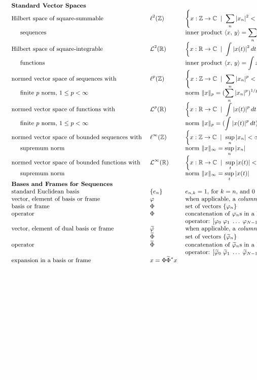
Standard Vector Spaces
Hilbert space of square-summable ℓ2(Z)
x : Z→ C |
∑
n
|xn|2 <∞
with
sequences inner product 〈x, y〉 =∑
n
xny∗n
Hilbert space of square-integrable L2(R)
x : R→ C |
∫|x(t)|2 dt <∞
with
functions inner product 〈x, y〉 =∫x(t)y(t)∗ dt
normed vector space of sequences with ℓp(Z)
x : Z→ C |
∑
n
|xn|p <∞
with
finite p norm, 1 ≤ p <∞ norm ‖x‖p = (∑
n
|xn|p)1/p
normed vector space of functions with Lp(R)x : R→ C |
∫|x(t)|p dt <∞
with
finite p norm, 1 ≤ p <∞ norm ‖x‖p = (
∫|x(t)|p dt)1/p
normed vector space of bounded sequences with ℓ∞(Z)
x : Z→ C | sup
n|xn| <∞
with
supremum norm norm ‖x‖∞ = supn|xn|
normed vector space of bounded functions with L∞(R)
x : R→ C | sup
t|x(t)| <∞
with
supremum norm norm ‖x‖∞ = supt|x(t)|
Bases and Frames for Sequencesstandard Euclidean basis en en,k = 1, for k = n, and 0 otherwisevector, element of basis or frame ϕ when applicable, a column vectorbasis or frame Φ set of vectors ϕnoperator Φ concatenation of ϕns in a linear
operator: [ϕ0 ϕ1 . . . ϕN−1]vector, element of dual basis or frame ϕ when applicable, a column vector
Φ set of vectors ϕnoperator Φ concatenation of ϕns in a linear
operator: [ϕ0 ϕ1 . . . ϕN−1]
expansion in a basis or frame x = ΦΦ∗x
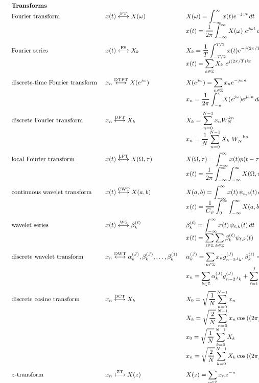
Transforms
Fourier transform x(t)FT←→ X(ω) X(ω) =
∫ ∞
−∞x(t)e−jωt dt
x(t) =1
2π
∫ ∞
−∞X(ω) ejωt dω
Fourier series x(t)FS←→ Xk Xk =
1
T
∫ T/2
−T/2x(t)e−j(2π/T )kt dt
x(t) =∑
k∈Z
Xk ej(2π/T )kt
discrete-time Fourier transform xnDTFT←→ X(ejω) X(ejω) =
∑
n∈Z
xne−jωn
xn =1
2π
∫ π
−πX(ejω)ejωn dω
discrete Fourier transform xnDFT←→ Xk Xk =
N−1∑
n=0
xnWknN
xn =1
N
N−1∑
n=0
Xk W−knN
local Fourier transform x(t)LFT←→ X(Ω, τ ) X(Ω, τ ) =
∫ ∞
−∞x(t)p(t− τ )e−jΩt dt
x(t) =1
2π
∫ ∞
−∞
∫ ∞
−∞X(Ω, τ ) gΩ,τ (t) dΩ dτ
continuous wavelet transform x(t)CWT←→ X(a, b) X(a, b) =
∫ ∞
−∞x(t)ψa,b(t) dt
x(t) =1
Cψ
∫ ∞
0
∫ ∞
−∞X(a, b)ψa,b(t)
db da
a2
wavelet series x(t)WS←→ β
(ℓ)k β
(ℓ)k =
∫ ∞
−∞x(t)ψℓ,k(t) dt
x(t) =∑
ℓ∈Z
∑
k∈Z
β(ℓ)k ψℓ,k(t)
discrete wavelet transform xnDWT←→ α
(J)k , β
(J)k , . . . , β
(1)k α
(J)k =
∑
n∈Z
xng(J)
n−2Jk, β
(ℓ)k =
∑
n∈Z
xnh(ℓ)
n−2ℓk
xn =∑
k∈Z
α(J)k g
(J)
n−2Jk+
J∑
ℓ=1
∑
k∈Z
β(ℓ)k h
(ℓ)
n−2ℓk
discrete cosine transform xnDCT←→ Xk X0 =
√1
N
N−1∑
n=0
xn
Xk =
√2
N
N−1∑
n=0
xn cos ((2π/2N)k(n+ 1/2))
x0 =
√1
N
N−1∑
k=0
Xk
xn =
√2
N
N−1∑
k=0
Xk cos ((2π/2N)k(n+ 1/2))
z-transform xnZT←→ X(z) X(z) =
∑
n∈Z
xnz−n
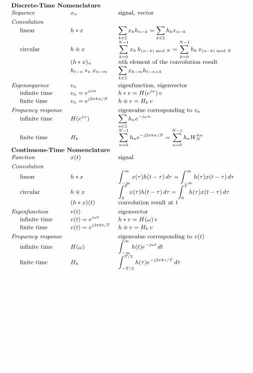
Discrete-Time NomenclatureSequence xn signal, vector
Convolution
linear h ∗ x∑
k∈Z
xkhn−k =∑
k∈Z
hkxn−k
circular h ⊛ x
N−1∑
k=0
xk h(n−k) mod N =
N−1∑
k=0
hk x(n−k) mod N
(h ∗ x)n nth element of the convolution result
hℓ−n ∗n xn−m∑
k∈Z
xk−mhℓ−n+k
Eigensequence vn eigenfunction, eigenvector
infinite time vn = ejωn h ∗ v = H(ejω) v
finite time vn = ej2πkn/N h ⊛ v = Hk v
Frequency response eigenvalue corresponding to vn
infinite time H(ejω)∑
n∈Z
hne−jωn
finite time Hk
N−1∑
n=0
hne−j2πkn/N =
N−1∑
n=0
hnWknN
Continuous-Time NomenclatureFunction x(t) signal
Convolution
linear h ∗ x∫ ∞
−∞x(τ )h(t− τ ) dτ =
∫ ∞
−∞h(τ )x(t− τ ) dτ
circular h ⊛ x
∫ T
0
x(τ )h(t− τ ) dτ =
∫ T
0
h(τ )x(t− τ ) dτ(h ∗ x)(t) convolution result at t
Eigenfunction v(t) eigenvector
infinite time v(t) = ejωt h ∗ v = H(ω) v
finite time v(t) = ej2πkt/T h ⊛ v = Hk v
Frequency response eigenvalue corresponding to v(t)
infinite time H(ω)
∫ ∞
−∞h(t)e−jωt dt
finite time Hk
∫ T/2
−T/2h(τ )e−j2πkτ/T dτ
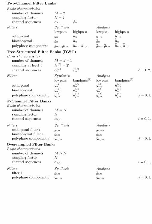
Two-Channel Filter Banks
Basic characteristicsnumber of channels M = 2sampling factor N = 2channel sequences αn βn
Filters Synthesis Analysislowpass highpass lowpass highpass
orthogonal gn hn g−n h−n
biorthogonal gn hn gn hnpolyphase components g0,n, g1,n h0,n, h1,n g0,n, g1,n h0,n, h1,n
Tree-Structured Filter Banks (DWT)Basic characteristics
number of channels M = J + 1
sampling at level ℓ N (ℓ) = 2ℓ
channel sequences α(J)n β(ℓ)
n ℓ = 1, 2, . . . , J
Filters Synthesis Analysis
lowpass bandpass(ℓ) lowpass bandpass(ℓ)
orthogonal g(J)n h(ℓ)n g
(J)−n h
(ℓ)−n
biorthogonal g(J)n h(ℓ)n g(J)n h(ℓ)
n
polyphase component j g(J)j,n h
(ℓ)j,n g
(J)j,n h
(ℓ)j,n j = 0, 1, . . . , 2ℓ − 1
N-Channel Filter BanksBasic characteristics
number of channels M = Nsampling factor Nchannel sequences αi,n i = 0, 1, . . . , N − 1
Filters Synthesis Analysisorthogonal filter i gi,n gi,−nbiorthogonal filter i gi,n gi,npolyphase component j gi,j,n gi,j,n j = 0, 1, . . . , N − 1
Oversampled Filter BanksBasic characteristics
number of channels M > Nsampling factor Nchannel sequences αi,n i = 0, 1, . . . ,M − 1
Filters Synthesis Analysisfilter i gi,n gi,npolyphase component j gi,j,n gi,j,n j = 0, 1, . . . , N − 1
Preface
The aim of this book, together with its predecessor Signal Processing: Foundations(SP:F) [107], is to provide a set of tools for users of state-of-the-art signal processingtechnology and a solid foundation for those hoping to advance the theory and prac-tice of signal processing. Many of the results and techniques presented here, whilerooted in classic Fourier techniques for signal representation, first appeared duringa flurry of activity in the 1980s and 1990s. New constructions for local Fouriertransforms and orthonormal wavelet bases during that period were motivated bothby theoretical interest and by applications, in particular in multimedia communica-tions. New bases with specified time–frequency behavior were found, with impactwell beyond the original fields of application. Areas as diverse as computer graphicsand numerical analysis embraced some of the new constructions—no surprise giventhe pervasive role of Fourier analysis in science and engineering.
Now that the dust has settled, some of what was new and esoteric is nowfundamental. Our motivation is to bring these new fundamentals to a broaderaudience to further expand their impact. We thus provide an integrated view ofclassical Fourier analysis of signals and systems alongside structured representationswith time–frequency locality and their myriad of applications.
This book relies heavily on the base built in SP:F. Thus, these two booksare to be seen as integrally related to each other. References to SP:F are given initalics.
Signal Processing: Foundations The first book covers the foundations for an ex-tensive understanding of signal processing. It contains material that many readersmay have seen before, but without the Hilbert space interpretations that are es-sential in contemporary signal processing research and technology. In Chapter 2,From Euclid to Hilbert, the basic geometric intuition central to Hilbert spaces is de-veloped, together with all the necessary tools underlying the construction of bases.Chapter 3, Sequences and Discrete-Time Systems, is a crash course on processingsignals in discrete time or discrete space. In Chapter 4, Functions and Continuous-Time Systems, the mathematics of Fourier transforms and Fourier series is reviewed.Chapter 5, Sampling and Interpolation, talks about the critical link between discreteand continuous domains as given by the sampling theorem and interpolation, whileChapter 6, Approximation and Compression, veers from the exact world to the ap-proximate one. The final chapter is Chapter 7, Localization and Uncertainty, and
it considers time–frequency behavior of the abstract representation objects studiedthus far. It also discusses issues arising in the real world as well as ways of adaptingthese tools for use in the real world. The main concepts seen—such as geometry ofHilbert spaces, existence of bases, Fourier representations, sampling and interpola-tion, and approximation and compression—build a powerful foundation for modernsignal processing. These tools hit roadblocks they must overcome: finiteness andlocalization, limitations of uncertainty, and computational costs.
Signal Processing: Fourier and Wavelet Representations This book presentssignal representations, including Fourier, local Fourier and wavelet bases, relatedconstructions, as well as frames and continuous transforms.
It starts with Chapter 1, Filter Banks: Building Blocks of Time-Frequency Ex-pansions, which presents a thorough treatment of the basic block—the two-channelfilter bank, a signal processing device that splits a signal into a coarse, lowpassapproximation, and a highpass detail.
We generalize this block in the three chapters that follow, all dealing withFourier- and wavelet-like representations on sequences: In Chapter 2, Local FourierBases on Sequences, we discuss Fourier-like bases on sequences, implemented byN -channel modulated filter banks (first generalization of the two-channel filterbanks). In Chapter 3, Wavelet Bases on Sequences, we discuss wavelet-like baseson sequences, implemented by tree-structured filter banks (second generalization).In Chapter 4, Local Fourier and Wavelet Frames on Sequences, we discuss bothFourier- and wavelet-like frames on sequences, implemented by oversampled filterbanks (third generalization).
We then move to the two chapters dealing with Fourier- and wavelet-like rep-resentations on functions. In Chapter 5, Local Fourier Transforms, Frames andBases on Functions, we start with the most natural representation of smooth func-tions with some locality, the local Fourier transform, followed by its sampled ver-sion/frame, and leading to results on whether bases are possible. In Chapter 6,Wavelet Bases, Frames and Transforms on Functions, we do the same for waveletrepresentations on functions, but in opposite order: starting from bases, throughframes and finally continuous wavelet transform.
The last chapter, Chapter 7, Approximation, Estimation, and Compression,uses all the tools we introduced to address state-of-the-art signal processing andcommunication problems and their solutions. The guiding principle is that there isa domain where the problem at hand will have a sparse solution, at least approxi-mately so. This is known as sparse signal processing, and many examples, from theclassical Karhunen-Loeve expansion to nonlinear approximation in discrete cosinetransform and wavelet domains, all the way to contemporary research in compressedsensing, use this principle. The chapter introduces and overviews sparse signal pro-cessing, covering approximation methods, estimation procedures such as denoising,as well as compression methods and inverse problems.
Teaching Points Our aim is to present a synthetic view from basic mathemati-cal principles to actual constructions of bases and frames, always with an eye on
concrete applications. While the benefit is a self-contained presentation, the costis a rather sizable manuscript. Referencing in the main text is sparse; pointers tobibliography are given in Further Reading at the end of each chapter.
The material grew out of teaching signal processing, wavelets and applicationsin various settings. Two of the authors, Martin Vetterli and Jelena Kovacevic, au-thored a graduate textbook, Wavelets and Subband Coding (originally with PrenticeHall in 1995), which they and others used to teach graduate courses at various USand European institutions. This book is now online with open access.1 With morethan a decade of experience, the maturing of the field, and the broader interestarising from and for these topics, the time was right for an entirely new text gearedtowards a broader audience, one that could be used to span levels from undergrad-uate to graduate, as well as various areas of engineering and science. As a case inpoint, parts of the text have been used at Carnegie Mellon University in classeson bioimage informatics, where some of the students are life-sciences majors. Thisplasticity of the text is one of the features which we aimed for, and that most prob-ably differentiates the present book from many others. Another aim is to presentside-by-side all methods that arose around signal representations, without favoringany in particular. The truth is that each representation is a tool in the toolbox ofthe practitioner, and the problem or application at hand ultimately determines theappropriate one to use.
Free Version This free, electronic version of the book contains all of the mainmaterial, except for solved exercises and exercises. Consequently, all references toexercises will show as ??. Moreover, this version does not contain PDF hyperlinks.
Jelena Kovacevic, Vivek K Goyaland Martin VetterliMarch 2012
1http://waveletsandsubbandcoding.org/
Chapter 1
Filter Banks: Building
Blocks of Time-Frequency
Expansions
Contents
1.1 Introduction 2
1.2 Orthogonal Two-Channel Filter Banks 7
1.3 Design of Orthogonal Two-Channel Filter Banks 20
1.4 Biorthogonal Two-Channel Filter Banks 26
1.5 Design of Biorthogonal Two-Channel Filter Banks 37
1.6 Two-Channel Filter Banks with Stochastic Inputs 41
1.7 Computational Aspects 42
Chapter at a Glance 49
Historical Remarks 52
Further Reading 52
The aim of this chapter is to build discrete-time bases with desirable time-frequency features and structure that enable tractable analysis and efficient algo-rithmic implementation. We achieve these goals by constructing bases via filterbanks.
Using filter banks provides an easy way to understand the relationship betweenanalysis and synthesis operators, while, at the same time, making their efficientimplementation obvious. Moreover, filter banks are at the root of the constructionsof wavelet bases in Chapters 3 and 6. In short, together with discrete-time filtersand the FFT, filter banks are among the most basic tools of signal processing.
This chapter deals exclusively with two-channel filter banks since they are(1) the simplest; (2) reveal the essence of the N -channel ones; and (3) are usedas building blocks for more general bases. We focus first on the orthogonal case,which is the most structured and has the easiest geometric interpretation. Dueto its importance in practice, we follow with the discussion of the biorthogonalcase. We consider real-coefficient filter banks exclusively; pointers to complex-coefficient ones, as well as to various generalizations, such as N -channel filter banks,multidimensional filter banks and transmultiplexers, are given in Further Reading.
1
2 Chapter 1. Filter Banks: Building Blocks of Time-Frequency Expansions
1.1 Introduction
Implementing a Haar Orthonormal Basis Expansion
At the end of the previous book, we constructed an orthonormal basis for ℓ2(Z)which possesses structure in terms of time and frequency localization properties(it serves as an almost perfect localization tool in time, and a rather rough one infrequency); and, is efficient (it is built from two template sequences, one lowpassand the other highpass, and their shifts). This was the so-called Haar basis.
What we want to do now is implement that basis using signal processingmachinery. We first rename our template basis sequences from (??) and (??) as:
gn = ϕ0,n = 1√2(δn + δn−1), (1.1a)
hn = ϕ1,n = 1√2(δn − δn−1). (1.1b)
This is done both for simplicity, as well as because it is the standard way thesesequences are denoted. We start by rewriting the reconstruction formula (??) as
xn =∑
k∈Z
〈x, ϕ2k〉︸ ︷︷ ︸αk
ϕ2k,n +∑
k∈Z
〈x, ϕ2k+1〉︸ ︷︷ ︸βk
ϕ2k+1,n
=∑
k∈Z
αk ϕ2k,n︸ ︷︷ ︸gn−2k
+∑
k∈Z
βk ϕ2k+1,n︸ ︷︷ ︸hn−2k
=∑
k∈Z
αkgn−2k +∑
k∈Z
βkhn−2k, (1.2)
where we have renamed the basis functions as in (1.1), as well as denoted theexpansion coefficients as
〈x, ϕ2k〉 = 〈xn, gn−2k〉n = αk, (1.3a)
〈x, ϕ2k+1〉 = 〈xn, hn−2k〉n = βk. (1.3b)
Then, recognize each sum in (1.2) as the output of upsampling followed by filtering(3.203) with the input sequences being αk and βk, respectively. Thus, the first sumin (1.2) can be implemented as the input sequence α going through an upsampler by2 followed by filtering by g, and the second as the input sequence β going throughan upsampler by 2 followed by filtering by h.
By the same token, we can identify the computation of the expansion coeffi-cients in (1.3) as (3.200), that is, both α and β sequences can be obtained usingfiltering by g−n followed by downsampling by 2 (for αk), or filtering by h−n followedby downsampling by 2 (for βk).
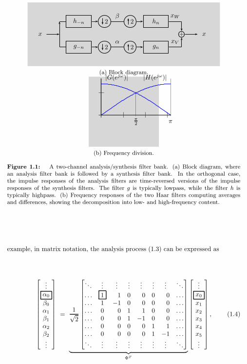
We can put together the above operations to yield a two-channel filter bankimplementing a Haar orthonormal basis expansion as in Figure 1.1(a). The left partthat computes the expansion coefficients is termed an analysis filter bank, while theright part that computes the projections is termed a synthesis filter bank.
As before, once we have identified all the appropriate multirate components,we can examine the Haar filter bank via matrix operations (linear operators). For
1.1. Introduction 3
x
h−n 2β
2 hn
g−n 2α
2 gn
xW
xV+ x
(a) Block diagram.
π
2 π
|G(ejω)| |H(ejω)|
(b) Frequency division.
Figure 1.1: A two-channel analysis/synthesis filter bank. (a) Block diagram, wherean analysis filter bank is followed by a synthesis filter bank. In the orthogonal case,the impulse responses of the analysis filters are time-reversed versions of the impulseresponses of the synthesis filters. The filter g is typically lowpass, while the filter h istypically highpass. (b) Frequency responses of the two Haar filters computing averagesand differences, showing the decomposition into low- and high-frequency content.
example, in matrix notation, the analysis process (1.3) can be expressed as
...α0
β0α1
β1α2
β2...
=1√2
. . ....
......
......
.... . .
. . . 1 1 0 0 0 0 . . .
. . . 1 −1 0 0 0 0 . . .
. . . 0 0 1 1 0 0 . . .
. . . 0 0 1 −1 0 0 . . .
. . . 0 0 0 0 1 1 . . .
. . . 0 0 0 0 1 −1 . . .
. . ....
......
......
.... . .
︸ ︷︷ ︸ΦT
...x0x1x2x3x4x5...
, (1.4)
4 Chapter 1. Filter Banks: Building Blocks of Time-Frequency Expansions
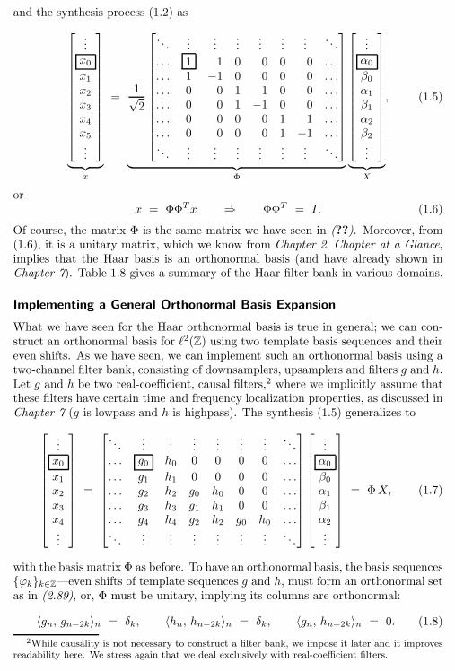
and the synthesis process (1.2) as
...x0x1x2x3x4x5...
︸ ︷︷ ︸x
=1√2
. . ....
......
......
.... . .
. . . 1 1 0 0 0 0 . . .
. . . 1 −1 0 0 0 0 . . .
. . . 0 0 1 1 0 0 . . .
. . . 0 0 1 −1 0 0 . . .
. . . 0 0 0 0 1 1 . . .
. . . 0 0 0 0 1 −1 . . .
. . ....
......
......
.... . .
︸ ︷︷ ︸Φ
...α0
β0α1
β1α2
β2...
︸ ︷︷ ︸X
, (1.5)
orx = ΦΦTx ⇒ ΦΦT = I. (1.6)
Of course, the matrix Φ is the same matrix we have seen in (??). Moreover, from(1.6), it is a unitary matrix, which we know from Chapter 2, Chapter at a Glance,implies that the Haar basis is an orthonormal basis (and have already shown inChapter 7). Table 1.8 gives a summary of the Haar filter bank in various domains.
Implementing a General Orthonormal Basis Expansion
What we have seen for the Haar orthonormal basis is true in general; we can con-struct an orthonormal basis for ℓ2(Z) using two template basis sequences and theireven shifts. As we have seen, we can implement such an orthonormal basis using atwo-channel filter bank, consisting of downsamplers, upsamplers and filters g and h.Let g and h be two real-coefficient, causal filters,2 where we implicitly assume thatthese filters have certain time and frequency localization properties, as discussed inChapter 7 (g is lowpass and h is highpass). The synthesis (1.5) generalizes to
...x0x1x2x3x4...
=
. . ....
......
......
.... . .
. . . g0 h0 0 0 0 0 . . .
. . . g1 h1 0 0 0 0 . . .
. . . g2 h2 g0 h0 0 0 . . .
. . . g3 h3 g1 h1 0 0 . . .
. . . g4 h4 g2 h2 g0 h0 . . .
. . ....
......
......
.... . .
...α0
β0α1
β1α2
...
= ΦX, (1.7)
with the basis matrix Φ as before. To have an orthonormal basis, the basis sequencesϕkk∈Z—even shifts of template sequences g and h, must form an orthonormal setas in (2.89), or, Φ must be unitary, implying its columns are orthonormal:
〈gn, gn−2k〉n = δk, 〈hn, hn−2k〉n = δk, 〈gn, hn−2k〉n = 0. (1.8)
2While causality is not necessary to construct a filter bank, we impose it later and it improvesreadability here. We stress again that we deal exclusively with real-coefficient filters.
1.1. Introduction 5
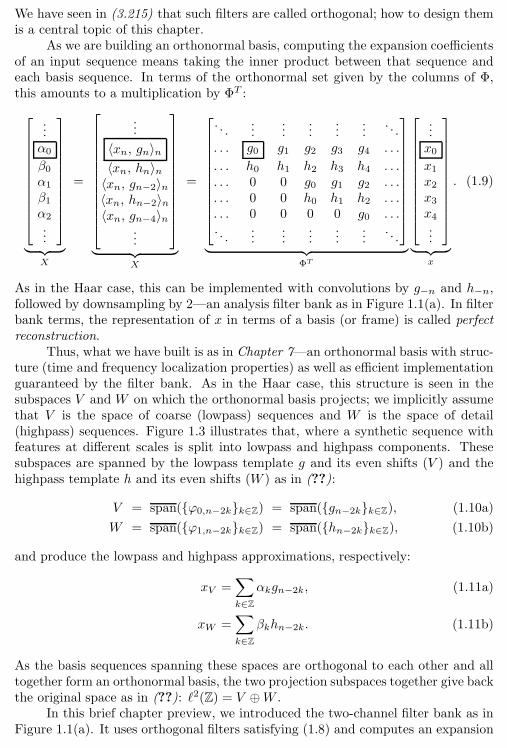
We have seen in (3.215) that such filters are called orthogonal; how to design themis a central topic of this chapter.
As we are building an orthonormal basis, computing the expansion coefficientsof an input sequence means taking the inner product between that sequence andeach basis sequence. In terms of the orthonormal set given by the columns of Φ,this amounts to a multiplication by ΦT :
...α0
β0α1
β1α2
...
︸ ︷︷ ︸X
=
...
〈xn, gn〉n〈xn, hn〉n〈xn, gn−2〉n〈xn, hn−2〉n〈xn, gn−4〉n
...
︸ ︷︷ ︸X
=
. . ....
......
......
. . .
. . . g0 g1 g2 g3 g4 . . .
. . . h0 h1 h2 h3 h4 . . .
. . . 0 0 g0 g1 g2 . . .
. . . 0 0 h0 h1 h2 . . .
. . . 0 0 0 0 g0 . . .
. . ....
......
......
. . .
︸ ︷︷ ︸ΦT
...x0x1x2x3x4...
︸ ︷︷ ︸x
. (1.9)
As in the Haar case, this can be implemented with convolutions by g−n and h−n,followed by downsampling by 2—an analysis filter bank as in Figure 1.1(a). In filterbank terms, the representation of x in terms of a basis (or frame) is called perfectreconstruction.
Thus, what we have built is as in Chapter 7—an orthonormal basis with struc-ture (time and frequency localization properties) as well as efficient implementationguaranteed by the filter bank. As in the Haar case, this structure is seen in thesubspaces V and W on which the orthonormal basis projects; we implicitly assumethat V is the space of coarse (lowpass) sequences and W is the space of detail(highpass) sequences. Figure 1.3 illustrates that, where a synthetic sequence withfeatures at different scales is split into lowpass and highpass components. Thesesubspaces are spanned by the lowpass template g and its even shifts (V ) and thehighpass template h and its even shifts (W ) as in (??):
V = span(ϕ0,n−2kk∈Z) = span(gn−2kk∈Z), (1.10a)
W = span(ϕ1,n−2kk∈Z) = span(hn−2kk∈Z), (1.10b)
and produce the lowpass and highpass approximations, respectively:
xV =∑
k∈Z
αkgn−2k, (1.11a)
xW =∑
k∈Z
βkhn−2k. (1.11b)
As the basis sequences spanning these spaces are orthogonal to each other and alltogether form an orthonormal basis, the two projection subspaces together give backthe original space as in (??): ℓ2(Z) = V ⊕W .
In this brief chapter preview, we introduced the two-channel filter bank as inFigure 1.1(a). It uses orthogonal filters satisfying (1.8) and computes an expansion
6 Chapter 1. Filter Banks: Building Blocks of Time-Frequency Expansions
V
W
x
xV
xW
l2(Z)
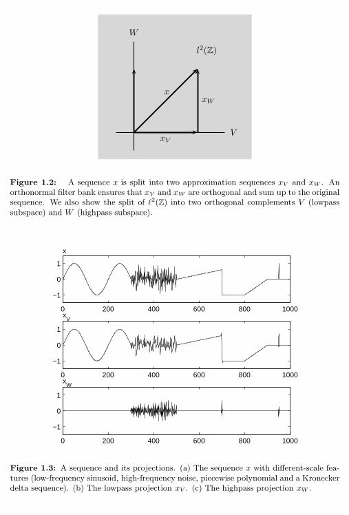
Figure 1.2: A sequence x is split into two approximation sequences xV and xW . Anorthonormal filter bank ensures that xV and xW are orthogonal and sum up to the originalsequence. We also show the split of ℓ2(Z) into two orthogonal complements V (lowpasssubspace) and W (highpass subspace).
0 200 400 600 800 1000
−1
0
1
x
0 200 400 600 800 1000
−1
0
1
xV
0 200 400 600 800 1000
−1
0
1
xW
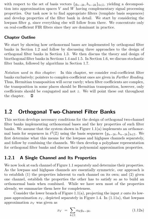
Figure 1.3: A sequence and its projections. (a) The sequence x with different-scale fea-tures (low-frequency sinusoid, high-frequency noise, piecewise polynomial and a Kroneckerdelta sequence). (b) The lowpass projection xV . (c) The highpass projection xW .
1.2. Orthogonal Two-Channel Filter Banks 7
with respect to the set of basis vectors gn−2k, hn−2kk∈Z, yielding a decomposi-tion into approximation spaces V and W having complementary signal processingproperties. Our task now is to find appropriate filters (template basis sequences)and develop properties of the filter bank in detail. We start by considering thelowpass filter g, since everything else will follow from there. We concentrate onlyon real-coefficient FIR filters since they are dominant in practice.
Chapter Outline
We start by showing how orthonormal bases are implemented by orthogonal filterbanks in Section 1.2 and follow by discussing three approaches to the design oforthogonal filter banks in Section 1.3. We then discuss the theory and design ofbiorthogonal filter banks in Sections 1.4 and 1.5. In Section 1.6, we discuss stochasticfilter banks, followed by algorithms in Section 1.7.
Notation used in this chapter: In this chapter, we consider real-coefficient filterbanks exclusively; pointers to complex-coefficient ones are given in Further Reading.Thus, Hermitian transposition will occur rarely; when filter coefficients are complex,the transposition in some places should be Hermitian transposition, however, onlycoefficients should be conjugated and not z. We will point these out throughoutthe chapter.
1.2 Orthogonal Two-Channel Filter Banks
This section develops necessary conditions for the design of orthogonal two-channelfilter banks implementing orthonormal bases and the key properties of such filterbanks. We assume that the system shown in Figure 1.1(a) implements an orthonor-mal basis for sequences in ℓ2(Z) using the basis sequences gn−2k, hn−2kk∈Z. Wefirst determine what this means for the lowpass and highpass channels separately,and follow by combining the channels. We then develop a polyphase representationfor orthogonal filter banks and discuss their polynomial approximation properties.
1.2.1 A Single Channel and Its Properties
We now look at each channel of Figure 1.1 separately and determine their properties.As the lowpass and highpass channels are essentially symmetric, our approach isto establish (1) the properties inherent to each channel on its own; and (2) givenone channel, establish the properties the other has to satisfy so as to build anorthonormal basis when combined. While we have seen most of the propertiesalready, we summarize them here for completeness.
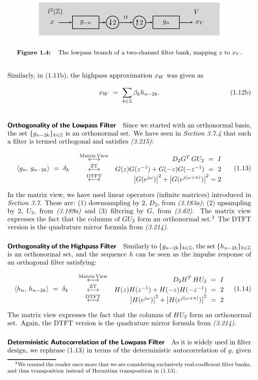
Consider the lower branch of Figure 1.1(a), projecting the input x onto its low-pass approximation xV , depicted separately in Figure 1.4. In (1.11a), that lowpassapproximation xV was given as
xV =∑
k∈Z
αkgn−2k. (1.12a)
8 Chapter 1. Filter Banks: Building Blocks of Time-Frequency Expansions
x
l2(Z)
g−n 2α
2 gn
V
xV
Figure 1.4: The lowpass branch of a two-channel filter bank, mapping x to xV .
Similarly, in (1.11b), the highpass approximation xW was given as
xW =∑
k∈Z
βkhn−2k. (1.12b)
Orthogonality of the Lowpass Filter Since we started with an orthonormal basis,the set gn−2kk∈Z is an orthonormal set. We have seen in Section 3.7.4 that sucha filter is termed orthogonal and satisfies (3.215):
〈gn, gn−2k〉 = δk
MatrixView←→ D2GT GU2 = I
ZT←→ G(z)G(z−1) +G(−z)G(−z−1) = 2DTFT←→
∣∣G(ejω)∣∣2 +
∣∣G(ej(ω+π))∣∣2 = 2
(1.13)
In the matrix view, we have used linear operators (infinite matrices) introduced inSection 3.7. These are: (1) downsampling by 2, D2, from (3.183a); (2) upsamplingby 2, U2, from (3.189a) and (3) filtering by G, from (3.62). The matrix viewexpresses the fact that the columns of GU2 form an orthonormal set.3 The DTFTversion is the quadrature mirror formula from (3.214).
Orthogonality of the Highpass Filter Similarly to gn−2kk∈Z, the set hn−2kk∈Z
is an orthonormal set, and the sequence h can be seen as the impulse response ofan orthogonal filter satisfying:
〈hn, hn−2k〉 = δk
MatrixView←→ D2HT HU2 = I
ZT←→ H(z)H(z−1) +H(−z)H(−z−1) = 2DTFT←→
∣∣H(ejω)∣∣2 +
∣∣H(ej(ω+π))∣∣2 = 2
(1.14)
The matrix view expresses the fact that the columns of HU2 form an orthonormalset. Again, the DTFT version is the quadrature mirror formula from (3.214).
Deterministic Autocorrelation of the Lowpass Filter As it is widely used in filterdesign, we rephrase (1.13) in terms of the deterministic autocorrelation of g, given
3We remind the reader once more that we are considering exclusively real-coefficient filter banks,and thus transposition instead of Hermitian transposition in (1.13).

1.2. Orthogonal Two-Channel Filter Banks 9
Lowpass Channel in a Two-Channel Orthogonal Filter Bank
Lowpass filter
Original domain gn 〈gn, gn−2k〉n = δkMatrix domain G D2G
T GU2 = I
z-domain G(z) G(z)G(z−1) +G(−z)G(−z−1) = 2
DTFT domain G(ejω) |G(ejω)|2 + |G(ej(ω+π))|2 = 2
(quadrature mirror formula)
Polyphase domain G(z) = G0(z2) + z−1G1(z
2) G0(z)G0(z−1) +G1(z)G1(z
−1) = 1
Deterministic autocorrelation
Original domain an = 〈gk, gk+n〉k a2k = δkMatrix domain A = GTG D2AU2 = I
z-domain A(z) = G(z)G(z−1) A(z) +A(−z) = 2
A(z) = 1 + 2∞∑
k=0
a2k+1(z2k+1 + z−(2k+1))
DTFT domain A(ejω) =∣∣G(ejω)
∣∣2 A(ejω) + A(ej(ω+π)) = 2
Orthogonal projection onto smooth space V = span(gn−2kk∈Z)
xV = PV x PV = GU2D2GT
Table 1.1: Properties of the lowpass channel in an orthogonal two-channel filter bank.Properties for the highpass channel are analogous.
by (3.96)):
〈gn, gn−2k〉 = a2k = δk
MatrixView←→ D2AU2 = IZT←→ A(z) +A(−z) = 2
DTFT←→ A(ejω) +A(ej(ω+π)) = 2
(1.15)
In the above, A = GTG is a symmetric matrix with element ak on the kth diagonalleft/right from the main diagonal. Thus, except for a0, all the other even terms ofak are 0, leading to
A(z)(a)= G(z)G(z−1) = 1 + 2
∞∑
k=0
a2k+1(z2k+1 + z−(2k+1)), (1.16)
where (a) follows from (3.143).
Deterministic Autocorrelation of the Highpass Filter Similarly to the lowpassfilter,
〈hn, hn−2k〉 = a2k = δk
MatrixView←→ D2AU2 = IZT←→ A(z) + A(−z) = 2
DTFT←→ A(ejω) +A(ej(ω+π)) = 2
(1.17)
Equation (1.16) holds for this deterministic autocorrelation as well.
10 Chapter 1. Filter Banks: Building Blocks of Time-Frequency Expansions
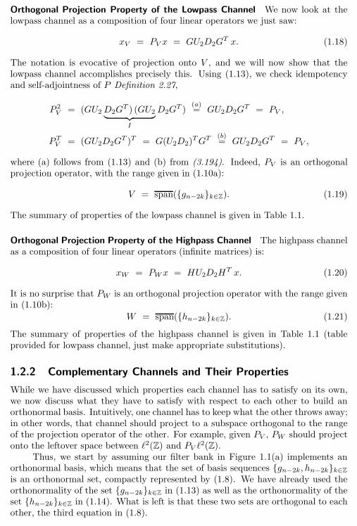
Orthogonal Projection Property of the Lowpass Channel We now look at thelowpass channel as a composition of four linear operators we just saw:
xV = PV x = GU2D2GT x. (1.18)
The notation is evocative of projection onto V , and we will now show that thelowpass channel accomplishes precisely this. Using (1.13), we check idempotencyand self-adjointness of P Definition 2.27,
P 2V
= (GU2D2GT ) (GU2︸ ︷︷ ︸I
D2GT )
(a)= GU2D2G
T = PV ,
PTV
= (GU2D2GT )T = G(U2D2)
TGT(b)= GU2D2G
T = PV ,
where (a) follows from (1.13) and (b) from (3.194). Indeed, PV is an orthogonalprojection operator, with the range given in (1.10a):
V = span(gn−2kk∈Z). (1.19)
The summary of properties of the lowpass channel is given in Table 1.1.
Orthogonal Projection Property of the Highpass Channel The highpass channelas a composition of four linear operators (infinite matrices) is:
xW = PWx = HU2D2HT x. (1.20)
It is no surprise that PW is an orthogonal projection operator with the range givenin (1.10b):
W = span(hn−2kk∈Z). (1.21)
The summary of properties of the highpass channel is given in Table 1.1 (tableprovided for lowpass channel, just make appropriate substitutions).
1.2.2 Complementary Channels and Their Properties
While we have discussed which properties each channel has to satisfy on its own,we now discuss what they have to satisfy with respect to each other to build anorthonormal basis. Intuitively, one channel has to keep what the other throws away;in other words, that channel should project to a subspace orthogonal to the rangeof the projection operator of the other. For example, given PV , PW should projectonto the leftover space between ℓ2(Z) and PV ℓ
2(Z).Thus, we start by assuming our filter bank in Figure 1.1(a) implements an
orthonormal basis, which means that the set of basis sequences gn−2k, hn−2kk∈Z
is an orthonormal set, compactly represented by (1.8). We have already used theorthonormality of the set gn−2kk∈Z in (1.13) as well as the orthonormality of theset hn−2kk∈Z in (1.14). What is left is that these two sets are orthogonal to eachother, the third equation in (1.8).
1.2. Orthogonal Two-Channel Filter Banks 11
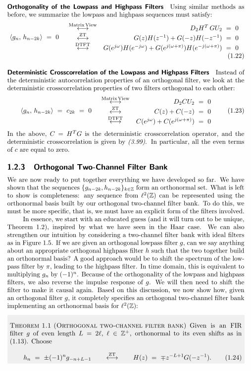
Orthogonality of the Lowpass and Highpass Filters Using similar methods asbefore, we summarize the lowpass and highpass sequences must satisfy:
〈gn, hn−2k〉 = 0
MatrixView←→ D2HT GU2 = 0
ZT←→ G(z)H(z−1) +G(−z)H(−z−1) = 0DTFT←→ G(ejω)H(e−jω) +G(ej(ω+π))H(e−j(ω+π)) = 0
(1.22)
Deterministic Crosscorrelation of the Lowpass and Highpass Filters Instead ofthe deterministic autocorrelation properties of an orthogonal filter, we look at thedeterministic crosscorrelation properties of two filters orthogonal to each other:
〈gn, hn−2k〉 = c2k = 0
MatrixView←→ D2CU2 = 0ZT←→ C(z) + C(−z) = 0
DTFT←→ C(ejω) + C(ej(ω+π)) = 0
(1.23)
In the above, C = HTG is the deterministic crosscorrelation operator, and thedeterministic crosscorrelation is given by (3.99). In particular, all the even termsof c are equal to zero.
1.2.3 Orthogonal Two-Channel Filter Bank
We are now ready to put together everything we have developed so far. We haveshown that the sequences gn−2k, hn−2kk∈Z form an orthonormal set. What is leftto show is completeness: any sequence from ℓ2(Z) can be represented using theorthonormal basis built by our orthogonal two-channel filter bank. To do this, wemust be more specific, that is, we must have an explicit form of the filters involved.
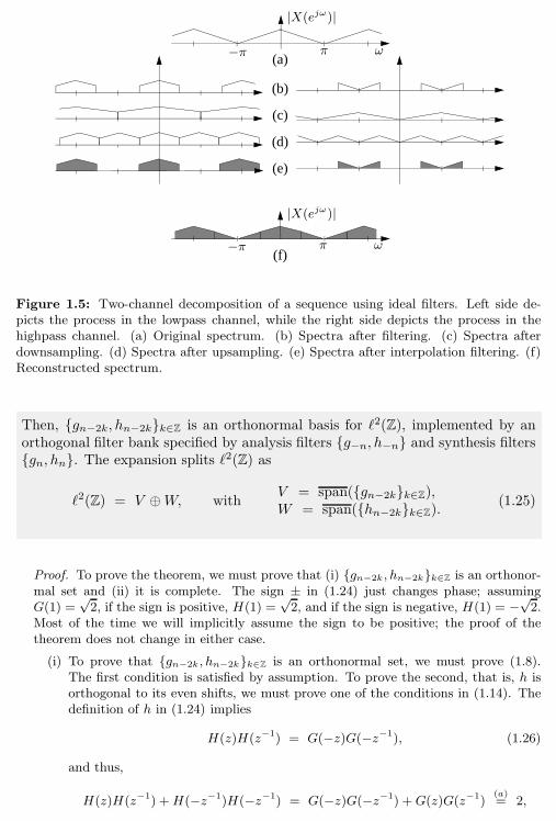
In essence, we start with an educated guess (and it will turn out to be unique,Theorem 1.2), inspired by what we have seen in the Haar case. We can alsostrengthen our intuition by considering a two-channel filter bank with ideal filtersas in Figure 1.5. If we are given an orthogonal lowpass filter g, can we say anythingabout an appropriate orthogonal highpass filter h such that the two together buildan orthonormal basis? A good approach would be to shift the spectrum of the low-pass filter by π, leading to the highpass filter. In time domain, this is equivalent tomultiplying gn by (−1)n. Because of the orthogonality of the lowpass and highpassfilters, we also reverse the impulse response of g. We will then need to shift thefilter to make it causal again. Based on this discussion, we now show how, givenan orthogonal filter g, it completely specifies an orthogonal two-channel filter bankimplementing an orthonormal basis for ℓ2(Z):
Theorem 1.1 (Orthogonal two-channel filter bank) Given is an FIRfilter g of even length L = 2ℓ, ℓ ∈ Z+, orthonormal to its even shifts as in(1.13). Choose
hn = ±(−1)ng−n+L−1ZT←→ H(z) = ∓z−L+1G(−z−1). (1.24)
12 Chapter 1. Filter Banks: Building Blocks of Time-Frequency Expansions
(b)
(c)
(d)
(e)
(f)
(a)
ω
ω
|X(ejω)|
|X(ejω)|
π
π
−π
−π
Figure 1.5: Two-channel decomposition of a sequence using ideal filters. Left side de-picts the process in the lowpass channel, while the right side depicts the process in thehighpass channel. (a) Original spectrum. (b) Spectra after filtering. (c) Spectra afterdownsampling. (d) Spectra after upsampling. (e) Spectra after interpolation filtering. (f)Reconstructed spectrum.
Then, gn−2k, hn−2kk∈Z is an orthonormal basis for ℓ2(Z), implemented by anorthogonal filter bank specified by analysis filters g−n, h−n and synthesis filtersgn, hn. The expansion splits ℓ2(Z) as
ℓ2(Z) = V ⊕W, withV = span(gn−2kk∈Z),W = span(hn−2kk∈Z).
(1.25)
Proof. To prove the theorem, we must prove that (i) gn−2k, hn−2kk∈Z is an orthonor-mal set and (ii) it is complete. The sign ± in (1.24) just changes phase; assumingG(1) =
√2, if the sign is positive, H(1) =
√2, and if the sign is negative, H(1) = −
√2.
Most of the time we will implicitly assume the sign to be positive; the proof of thetheorem does not change in either case.
(i) To prove that gn−2k, hn−2kk∈Z is an orthonormal set, we must prove (1.8).The first condition is satisfied by assumption. To prove the second, that is, h isorthogonal to its even shifts, we must prove one of the conditions in (1.14). Thedefinition of h in (1.24) implies
H(z)H(z−1) = G(−z)G(−z−1), (1.26)
and thus,
H(z)H(z−1) +H(−z−1)H(−z−1) = G(−z)G(−z−1) +G(z)G(z−1)(a)= 2,
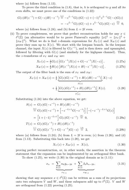
1.2. Orthogonal Two-Channel Filter Banks 13
where (a) follows from (1.13).To prove the third condition in (1.8), that is, h is orthogonal to g and all its
even shifts, we must prove one of the conditions in (1.22):
G(z)H(z−1) +G(−z)H(−z−1)(a)= −zL−1G(z)G(−z) + (−1)LzL−1G(−z)G(z)
= −zL−1G(z)G(−z) + zL−1G(z)G(−z) (b)= 0,
where (a) follows from (1.24); and (b) from L = 2ℓ even.
(ii) To prove completeness, we prove that perfect reconstruction holds for any x ∈ℓ2(Z) (an alternative would be to prove Parseval’s equality ‖x‖2 = ‖xV ‖2 +‖xW ‖2). What we do is find z-domain expressions for XV (z) and XW (z) andprove they sum up to X(z). We start with the lowpass branch. In the lowpasschannel, the input X(z) is filtered by G(z−1), and is then down- and upsampled,followed by filtering with G(z) (and similarly for the highpass channel). Thus,the z-transforms of xV and xW are:
XV (z) =12G(z)
[G(z−1)X(z) +G(−z−1)X(−z)
], (1.27a)
XW (z) = 12H(z)
[H(z−1)X(z) +H(−z−1)X(−z)
]. (1.27b)
The output of the filter bank is the sum of xV and xW :
XV (z) +XW (z) = 12
[G(z)G(−z−1) +H(z)H(−z−1)
]︸ ︷︷ ︸
S(z)
X(−z)
+ 12
[G(z)G(z−1) +H(z)H(z−1)
]︸ ︷︷ ︸
T (z)
X(z). (1.28)
Substituting (1.24) into the above equation, we get:
S(z) = G(z)G(−z−1) +H(z)H(−z−1)
(a)= G(z)G(−z−1) +
[−z−L+1G(−z−1)
] [−(−z−1)−L+1G(z)
]
=[1 + (−1)−L+1
]G(z)G(−z−1)
(b)= 0, (1.29a)
T (z) = G(z)G(z−1) +H(z)H(z−1)
(c)= G(z)G(z−1) +G(−z−1)G(−z) (d)
= 2, (1.29b)
where (a) follows from (1.24); (b) from L = 2ℓ is even; (c) from (1.26); and (d)from (1.13). Substituting this back into (1.28), we get
XV (z) +XW (z) = X(z), (1.30)
proving perfect reconstruction, or, in other words, the assertion in the theoremstatement that the expansion can be implemented by an orthogonal filter bank.
To show (1.25), we write (1.30) in the original domain as in (1.11):
xn =∑
k∈Z
αkgn−2k
︸ ︷︷ ︸xV,n
+∑
k∈Z
βkhn−2k
︸ ︷︷ ︸xW,n
, (1.31)
showing that any sequence x ∈ ℓ2(Z) can be written as a sum of its projectionsonto two subspaces V and W , and these subspaces add up to ℓ2(Z). V and Ware orthogonal from (1.22) proving (1.25).
14 Chapter 1. Filter Banks: Building Blocks of Time-Frequency Expansions
In the theorem, L is an even integer, which is a requirement for FIR filters of lengthsgreater than 1 (see Exercise ??). Moreover, the choice (1.24) is unique; this willbe shown in Theorem 1.2. Table 1.9 summarizes various properties of orthogonal,two-channel filter banks we covered until now.
Along with the time reversal and shift, the other qualitative feature of (1.24)is modulation by ejnπ = (−1)n (mapping z → −z in the z domain, see (3.137)). Aswe said, this makes h a highpass filter when g is a lowpass filter. As an example,if we apply Theorem 1.1 to the Haar lowpass filter from (1.1a), we obtain the Haarhighpass filter from (1.1b).
In applications, filters are causal. To implement a filter bank with causalfilters, we make analysis filters causal (we already assumed the synthesis ones are)by shifting them both by (−L + 1). Beware that such an implementation impliesperfect reconstruction within a shift (delay), and the orthonormal basis expansionis not technically valid anymore. However, in applications this is often done, as theoutput sequence is a perfect replica of the input one, within a shift: xn = xn−L+1.
1.2.4 Polyphase View of Orthogonal Filter Banks
As we saw in Section 3.7, downsampling introduces periodic shift variance into thesystem. To deal with this, we often analyze multirate systems in polyphase domain,as discussed in Section 3.7.5. The net result is that the analysis of a single-input,single-output, periodically shift-varying system is equivalent to the analysis of amultiple-input, multiple-output, shift-invariant system.
Polyphase Representation of an Input Sequence For two-channel filter banks,a polyphase decomposition of the input sequence is achieved by simply splitting itinto its even- and odd-indexed subsequences as in (3.216), the main idea being thatthe sequence can be recovered from the two subsequences by upsampling, shiftingand summing up, as we have seen in Figure 3.29. This simple process is called apolyphase transform (forward and inverse).
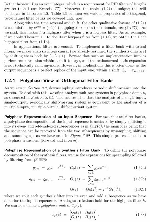
Polyphase Representation of a Synthesis Filter Bank To define the polyphasedecomposition of the synthesis filters, we use the expressions for upsampling followedby filtering from (3.220):
g0,n = g2nZT←→ G0(z) =
∑
n∈Z
g2nz−n, (1.32a)
g1,n = g2n+1ZT←→ G1(z) =
∑
n∈Z
g2n+1z−n, (1.32b)
G(z) = G0(z2) + z−1G1(z
2), (1.32c)
where we split each synthesis filter into its even and odd subsequence as we havedone for the input sequence x. Analogous relations hold for the highpass filter h.We can now define a polyphase matrix Φp(z):
Φp(z) =
[G0(z) H0(z)G1(z) H1(z)
]. (1.33)
1.2. Orthogonal Two-Channel Filter Banks 15
As we will see in (1.37), such a matrix allows for a compact representation, analysisand computing projections in the polyphase domain.
Polyphase Representation of an Analysis Filter Bank The matrix in (1.33) is onthe synthesis side; to get it on the analysis side, we can use the fact that this is anorthogonal filter bank. Thus, we can write
G(z) = G(z−1) = G0(z−2) + zG1(z
−2).
In other words, the polyphase components of the analysis filter are, not surprisingly,time-reversed versions of the polyphase components of the synthesis filter. We cansummarize this as (we could have obtained the same result using the expression forpolyphase representation of downsampling preceded by filtering (3.226)):
g0,n = g2n = g−2nZT←→ G0(z) =
∑
n∈Z
g−2nz−n, (1.34a)
g1,n = g2n−1 = g−2n+1ZT←→ G1(z) =
∑
n∈Z
g−2n+1z−n, (1.34b)
G(z) = G0(z−2) + zG1(z
−2), (1.34c)
with analogous relations for the highpass filter h, yielding the expression for theanalysis polyphase matrix
Φp(z) =
[G0(z) H0(z)
G1(z) H1(z)
]=
[G0(z
−1) H0(z−1)
G1(z−1) H1(z
−1)
]= Φp(z
−1). (1.35)
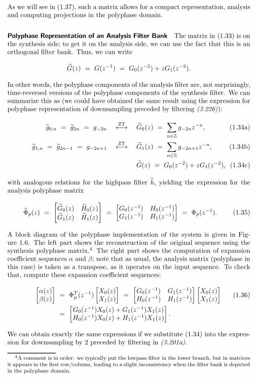
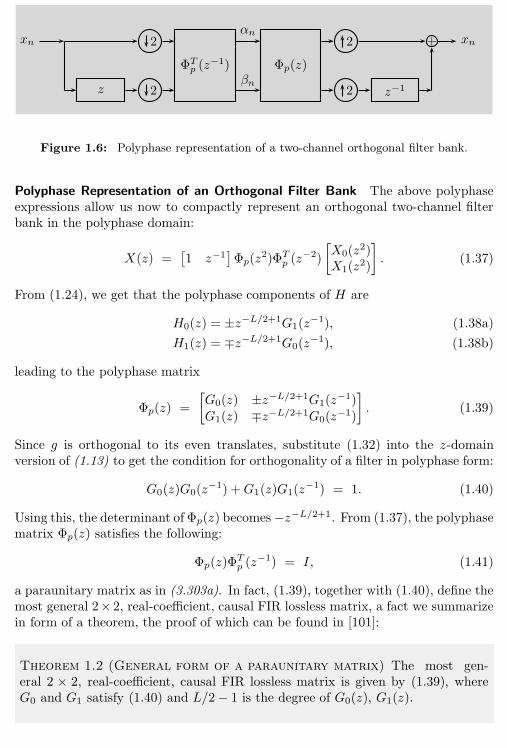
A block diagram of the polyphase implementation of the system is given in Fig-ure 1.6. The left part shows the reconstruction of the original sequence using thesynthesis polyphase matrix.4 The right part shows the computation of expansioncoefficient sequences α and β; note that as usual, the analysis matrix (polyphase inthis case) is taken as a transpose, as it operates on the input sequence. To checkthat, compute these expansion coefficient sequences:
[α(z)β(z)
]= ΦT
p(z−1)
[X0(z)X1(z)
]=
[G0(z
−1) G1(z−1)
H0(z−1) H1(z
−1)
] [X0(z)X1(z)
](1.36)
=
[G0(z
−1)X0(z) +G1(z−1)X1(z)
H0(z−1)X0(z) +H1(z
−1)X1(z)
].
We can obtain exactly the same expressions if we substitute (1.34) into the expres-sion for downsampling by 2 preceded by filtering in (3.201a).
4A comment is in order: we typically put the lowpass filter in the lower branch, but in matricesit appears in the first row/column, leading to a slight inconsistency when the filter bank is depictedin the polyphase domain.
16 Chapter 1. Filter Banks: Building Blocks of Time-Frequency Expansions
xn 2
ΦTp(z−1)
αn
Φp(z)
2 +
z 2βn
2 z−1
xn
Figure 1.6: Polyphase representation of a two-channel orthogonal filter bank.
Polyphase Representation of an Orthogonal Filter Bank The above polyphaseexpressions allow us now to compactly represent an orthogonal two-channel filterbank in the polyphase domain:
X(z) =[1 z−1
]Φp(z
2)ΦTp(z−2)
[X0(z
2)X1(z
2)
]. (1.37)
From (1.24), we get that the polyphase components of H are
H0(z) = ±z−L/2+1G1(z−1), (1.38a)
H1(z) = ∓z−L/2+1G0(z−1), (1.38b)
leading to the polyphase matrix
Φp(z) =
[G0(z) ±z−L/2+1G1(z
−1)G1(z) ∓z−L/2+1G0(z
−1)
]. (1.39)
Since g is orthogonal to its even translates, substitute (1.32) into the z-domainversion of (1.13) to get the condition for orthogonality of a filter in polyphase form:
G0(z)G0(z−1) +G1(z)G1(z
−1) = 1. (1.40)
Using this, the determinant of Φp(z) becomes−z−L/2+1. From (1.37), the polyphasematrix Φp(z) satisfies the following:
Φp(z)ΦT
p(z−1) = I, (1.41)
a paraunitary matrix as in (3.303a). In fact, (1.39), together with (1.40), define themost general 2× 2, real-coefficient, causal FIR lossless matrix, a fact we summarizein form of a theorem, the proof of which can be found in [101]:
Theorem 1.2 (General form of a paraunitary matrix) The most gen-eral 2 × 2, real-coefficient, causal FIR lossless matrix is given by (1.39), whereG0 and G1 satisfy (1.40) and L/2− 1 is the degree of G0(z), G1(z).
1.2. Orthogonal Two-Channel Filter Banks 17
Example 1.1 (Haar filter bank in polyphase form) The Haar filters (1.1)are extremely simple in polyphase form: Since they are both of length 2, theirpolyphase components are of length 1. The polyphase matrix is simply
Φp(z) =1√2
[1 11 −1
]. (1.42)
The form of the polyphase matrix for the Haar orthonormal basis is exactly thesame as the Haar orthonormal basis for R2, or one block of the Haar orthonormalbasis infinite matrix Φ from (??). This is true only when a filter bank implementsthe so-called block transform, that is, when the nonzero support of the basissequences is equal to the sampling factor, 2 in this case.
The polyphase notation and the associated matrices are powerful tools toderive filter bank results. We now rephrase what it means for a filter bank to beorthogonal—implement an orthonormal basis, in polyphase terms.
Theorem 1.3 (Paraunitary polyphase matrix and orthonormal basis)A 2 × 2 polyphase matrix Φp(z) is paraunitary if and only if the associatedtwo-channel filter bank implements an orthonormal basis for ℓ2(Z).
Proof. If the polyphase matrix is paraunitary, then the expansion it implements iscomplete, due to (1.41). To prove that the expansion is an orthonormal basis, we mustshow that the basis sequences form an orthonormal set. From (1.39) and (1.41), we get(1.40). Substituting this into the z-domain version of (1.13), we see that it holds, andthus g and its even shifts form an orthonormal set. Because h is given in terms of g as(1.24), h and its even shifts form an orthonormal set as well. Finally, because of theway h is defined, g and h are orthogonal by definition and so are their even shifts.
The argument in the other direction is similar; we start with an orthonormal basisimplemented by a two-channel filter bank. That means we have template sequences gand h related via (1.24), and their even shifts, all together forming an orthonormalbasis. We can now translate those conditions into z-transform domain using (1.13) andderive the corresponding polyphase-domain versions, such as the one in (1.40). Theselead to the polyphase matrix being paraunitary.
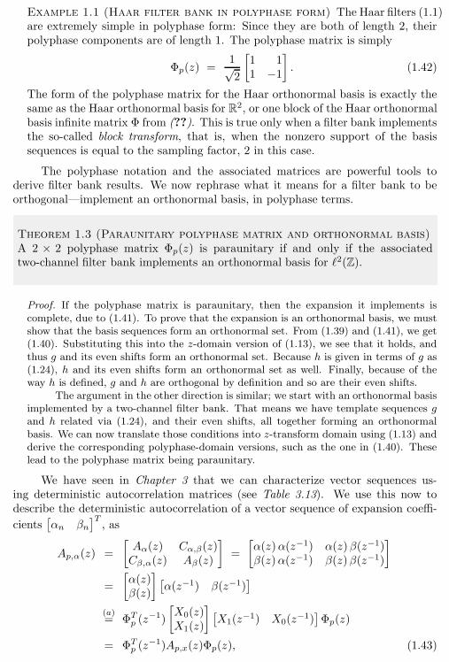
We have seen in Chapter 3 that we can characterize vector sequences us-ing deterministic autocorrelation matrices (see Table 3.13). We use this now todescribe the deterministic autocorrelation of a vector sequence of expansion coeffi-
cients[αn βn
]T
, as
Ap,α(z) =
[Aα(z) Cα,β(z)Cβ,α(z) Aβ(z)
]=
[α(z)α(z−1) α(z)β(z−1)β(z)α(z−1) β(z)β(z−1)
]
=
[α(z)β(z)
] [α(z−1) β(z−1)
]
(a)= ΦT
p(z−1)
[X0(z)X1(z)
] [X1(z
−1) X0(z−1)]Φp(z)
= ΦTp(z−1)Ap,x(z)Φp(z), (1.43)
18 Chapter 1. Filter Banks: Building Blocks of Time-Frequency Expansions
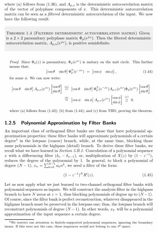
where (a) follows from (1.36), and Ap,x is the deterministic autocorrelation matrixof the vector of polyphase components of x. This deterministic autocorrelationmatrix can be seen as a filtered deterministic autocorrelation of the input. We nowhave the following result:
Theorem 1.4 (Filtered deterministic autocorrelation matrix) Givenis a 2× 2 paraunitary polyphase matrix Φp(e
jω). Then the filtered deterministicautocorrelation matrix, Ap,α(e
jω), is positive semidefinite.
Proof. Since Φp(z) is paraunitary, Φp(ejω) is unitary on the unit circle. This further
means that: [cos θ sin θ
]ΦTp (e
−jω) =[cosφ sinφ
], (1.44)
for some φ. We can now write:
[cos θ sin θ
]Ap,α(e
jω)
[cos θsin θ
](a)=
[cos θ sin θ
]ΦTp (e
−jω)Ap,x(ejω)Φp(e
jω)
[cos θsin θ
]
(b)=
[cos φ sinφ
]Ap,x(e
jω)
[cosφsinφ
](c)
≥ 0,
where (a) follows from (1.43); (b) from (1.44); and (c) from TBD, proving the theorem.
1.2.5 Polynomial Approximation by Filter Banks
An important class of orthogonal filter banks are those that have polynomial ap-proximation properties; these filter banks will approximate polynomials of a certaindegree5 in the lowpass (coarse) branch, while, at the same time, blocking thosesame polynomials in the highpass (detail) branch. To derive these filter banks, werecall what we have learned in Section 3.B.1: Convolution of a polynomial sequencex with a differencing filter (δn − δn−1), or, multiplication of X(z) by (1 − z−1),reduces the degree of the polynomial by 1. In general, to block a polynomial ofdegree (N − 1), xn =
∑N−1k=0 akn
k, we need a filter of the form:
(1− z−1)NR′(z). (1.45)
Let us now apply what we just learned to two-channel orthogonal filter banks withpolynomial sequences as inputs. We will construct the analysis filter in the highpassbranch to have N zeros at z = 1, thus blocking polynomials of degree up to (N−1).Of course, since the filter bank is perfect reconstruction, whatever disappeared in thehighpass branch must be preserved in the lowpass one; thus, the lowpass branch willreconstruct polynomials of degree (N − 1). In other words, xV will be a polynomialapproximation of the input sequence a certain degree.
5We restrict our attention to finitely-supported polynomial sequences, ignoring the boundaryissues. If this were not the case, these sequences would not belong to any ℓp space.
1.2. Orthogonal Two-Channel Filter Banks 19
To construct such a filter bank, we start with the analysis highpass filter hwhich must be of the form (1.45); we write it as:
H(z)(a)= (1− z−1)N ∓zL−1R(−z)︸ ︷︷ ︸
R′(z)
= ∓zL−1(1− z−1)NR(−z) (b)= ∓zL−1G(−z),
where in (a) we have chosen R′(z) to lead to a simple form of G(z) in what follows;and (b) follows from Table 1.9, allowing us to directly read the synthesis lowpass as
G(z) = (1 + z−1)NR(z). (1.46)
If we maintain the convention that g is causal and of length L, then R(z) is a poly-nomial in z−1 of degree (L−1−N). Of course, R(z) has to be chosen appropriately,so as to obtain an orthogonal filter bank.
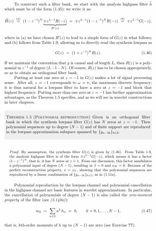
Putting at least one zero at z = −1 in G(z) makes a lot of signal processingsense. After all, z = −1 corresponds to ω = π, the maximum discrete frequency;it is thus natural for a lowpass filter to have a zero at z = −1 and block thathighest frequency. Putting more than one zero at z = −1 has further approximationadvantages, as the Theorem 1.5 specifies, and as we will see in wavelet constructionsin later chapters.
Theorem 1.5 (Polynomial reproduction) Given is an orthogonal filterbank in which the synthesis lowpass filter G(z) has N zeros at z = −1. Thenpolynomial sequences up to degree (N − 1) and of finite support are reproducedin the lowpass approximation subspace spanned by gn−2kk∈Z.
Proof. By assumption, the synthesis filter G(z) is given by (1.46). From Table 1.9,the analysis highpass filter is of the form ∓zL−1G(−z), which means it has a factor(1−z−1)N , that is, it has N zeros at z = 1. From our discussion, this factor annihilatesa polynomial input of degree (N − 1), resulting in β = 0 and xW = 0. Because of theperfect reconstruction property, x = xV , showing that the polynomial sequences arereproduced by a linear combination of gn−2kk∈Z, as in (1.11a).
Polynomial reproduction by the lowpass channel and polynomial cancellationin the highpass channel are basic features in wavelet approximations. In particular,the cancellation of polynomials of degree (N − 1) is also called the zero-momentproperty of the filter (see (3.140a)):
mk =∑
n∈Z
nk hn = 0, k = 0, 1, . . . , N − 1, (1.47)
that is, kth-order moments of h up to (N − 1) are zero (see Exercise ??).
20 Chapter 1. Filter Banks: Building Blocks of Time-Frequency Expansions
1.3 Design of Orthogonal Two-Channel Filter Banks
To design a two-channel orthogonal filter bank, it suffices to design one orthogonalfilter—the lowpass synthesis g with the z-transform G(z) satisfying (1.13); we haveseen how the other three filters follow (Table 1.9). The design is based on (1)finding a deterministic autocorrelation function satisfying (1.15) (it is symmetric,positive semi-definite and has a single nonzero even-indexed coefficient; and (2)factoring that deterministic autocorrelation A(z) = G(z)G(z−1) into its spectralfactors (many factorizations are possible, see Section 3.5).6
We consider three different designs. The first tries to approach an ideal half-band lowpass filter, the second aims at polynomial approximation, while the thirduses lattice factorization in polyphase domain.
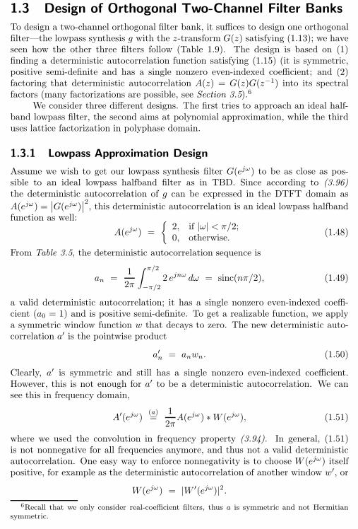
1.3.1 Lowpass Approximation Design
Assume we wish to get our lowpass synthesis filter G(ejω) to be as close as pos-sible to an ideal lowpass halfband filter as in TBD. Since according to (3.96)the deterministic autocorrelation of g can be expressed in the DTFT domain as
A(ejω) =∣∣G(ejω)
∣∣2, this deterministic autocorrelation is an ideal lowpass halfbandfunction as well:
A(ejω) =
2, if |ω| < π/2;0, otherwise.
(1.48)
From Table 3.5, the deterministic autocorrelation sequence is
an =1
2π
∫π/2
−π/22 ejnω dω = sinc(nπ/2), (1.49)
a valid deterministic autocorrelation; it has a single nonzero even-indexed coeffi-cient (a0 = 1) and is positive semi-definite. To get a realizable function, we applya symmetric window function w that decays to zero. The new deterministic auto-correlation a′ is the pointwise product
a′n
= anwn. (1.50)
Clearly, a′ is symmetric and still has a single nonzero even-indexed coefficient.However, this is not enough for a′ to be a deterministic autocorrelation. We cansee this in frequency domain,
A′(ejω)(a)=
1
2πA(ejω) ∗W (ejω), (1.51)
where we used the convolution in frequency property (3.94). In general, (1.51)is not nonnegative for all frequencies anymore, and thus not a valid deterministicautocorrelation. One easy way to enforce nonnegativity is to choose W (ejω) itselfpositive, for example as the deterministic autocorrelation of another window w′, or
W (ejω) = |W ′(ejω)|2.6Recall that we only consider real-coefficient filters, thus a is symmetric and not Hermitian
symmetric.
1.3. Design of Orthogonal Two-Channel Filter Banks 21
If w′ is of norm 1, then w0 = 1, and from (1.50), a′0 = 1 as well. Therefore, sinceA(ejω) is real and positive, A′(ejω) will be as well. The resulting sequence a′ andits z-transform A′(z) can then be used in spectral factorization (see Section 3.5.3)to obtain an orthogonal filter g.
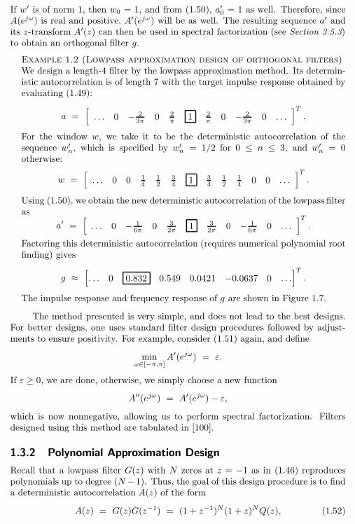
Example 1.2 (Lowpass approximation design of orthogonal filters)We design a length-4 filter by the lowpass approximation method. Its determin-istic autocorrelation is of length 7 with the target impulse response obtained byevaluating (1.49):
a =[. . . 0 − 2
3π 0 2π
1 2π
0 − 23π 0 . . .
]T
.
For the window w, we take it to be the deterministic autocorrelation of thesequence w′
n, which is specified by w′
n= 1/2 for 0 ≤ n ≤ 3, and w′
n= 0
otherwise:
w =[. . . 0 0 1
412
34 1 3
412
14 0 0 . . .
]T
.
Using (1.50), we obtain the new deterministic autocorrelation of the lowpass filteras
a′ =[. . . 0 − 1
6π 0 32π 1 3
2π 0 − 16π 0 . . .
]T
.
Factoring this deterministic autocorrelation (requires numerical polynomial rootfinding) gives
g ≈[. . . 0 0.832 0.549 0.0421 −0.0637 0 . . .
]T
.
The impulse response and frequency response of g are shown in Figure 1.7.
The method presented is very simple, and does not lead to the best designs.For better designs, one uses standard filter design procedures followed by adjust-ments to ensure positivity. For example, consider (1.51) again, and define
minω∈[−π,π]
A′(ejω) = ε.
If ε ≥ 0, we are done, otherwise, we simply choose a new function
A′′(ejω) = A′(ejω)− ε,
which is now nonnegative, allowing us to perform spectral factorization. Filtersdesigned using this method are tabulated in [100].
1.3.2 Polynomial Approximation Design
Recall that a lowpass filter G(z) with N zeros at z = −1 as in (1.46) reproducespolynomials up to degree (N − 1). Thus, the goal of this design procedure is to finda deterministic autocorrelation A(z) of the form
A(z) = G(z)G(z−1) = (1 + z−1)N (1 + z)NQ(z), (1.52)

22 Chapter 1. Filter Banks: Building Blocks of Time-Frequency Expansions
−2 0 2 4
−0.1
0
0.1
0.2
0.3
0.4
0.5
0.6
0.7
0.8
0.9
gn
0
0.2
0.4
0.6
0.8
1
1.2
1.4
|G(ejω)|
0 π/2 π
Figure 1.7: Orthogonal filter design based on lowpass approximation in Example 1.2.(a) Impulse response. (b) Frequency response.
with Q(z) chosen such that (1.15) is satisfied, that is,
A(z) +A(−z) = 2, (1.53)
Q(z) = Q(z−1) (qn symmetric in time domain), and Q(z) is nonnegative on theunit circle. Satisfying these conditions allows one to find a spectral factor of A(z)with N zeros at z = −1, and this spectral factor is the desired orthogonal filter.We illustrate this procedure through an example.
Example 1.3 (Polynomial approximation design of orthogonal filters)We will design a filter g such that it reproduces linear polynomials, that is, N = 2:
A(z) = (1 + z−1)2(1 + z)2Q(z) = (z−2 + 4z−1 + 6 + 4z + z2)Q(z).
Can we now find Q(z) so as to satisfy (1.53), in particular, a minimum-degreesolution? We try with (remember qn is symmetric)
Q(z) = az + b+ az−1
and compute A(z) as
A(z) = a(z3 + z−3) + (4a+ b)(z2 + z−2) + (7a+ 4b)(z + z−1) + (8a+ 6b).
To satisfy (1.53), A(z) must have a single nonzero even-indexed coefficient. Wethus need to solve the following pair of equations:
4a+ b = 0,
8a+ 6b = 1,
yielding a = −1/16 and b = 1/4. Thus, our candidate factor is
Q(z) =1
4
(−1
4z−1 + 1− 1
4z
).
1.3. Design of Orthogonal Two-Channel Filter Banks 23
−0.2
0
0.2
0.4
0.6
0.8
1
1.2
0
0.5
1
1.5|G(ejω)|
π/2 π
gn
(a) (b)
(c) (d)
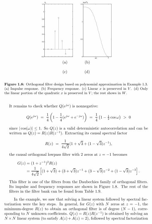
Figure 1.8: Orthogonal filter design based on polynomial approximation in Example 1.3.(a) Impulse response. (b) Frequency response. (c) Linear x is preserved in V . (d) Onlythe linear portion of the quadratic x is preserved in V ; the rest shows in W .
It remains to check whether Q(ejω) is nonnegative:
Q(ejω) =1
4
(1− 1
4(ejω + e−jω)
)=
1
4
(1− 1
2 cosω)> 0
since | cos(ω)| ≤ 1. So Q(z) is a valid deterministic autocorrelation and can bewritten as Q(z) = R(z)R(z−1). Extracting its causal spectral factor
R(z) =1
4√2(1 +
√3 + (1 −
√3)z−1),
the causal orthogonal lowpass filter with 2 zeros at z = −1 becomes
G(z) = (1 + z−1)2R(z)
=1
4√2
[(1 +
√3) + (3 +
√3)z−1 + (3−
√3)z−2 + (1−
√3)z−3
].
This filter is one of the filters from the Daubechies family of orthogonal filters.Its impulse and frequency responses are shown in Figure 1.8. The rest of thefilters in the filter bank can be found from Table 1.9.
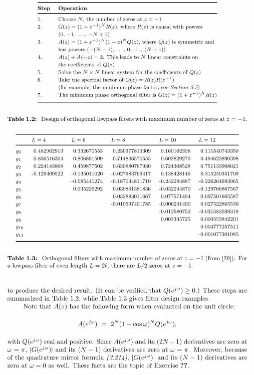
In the example, we saw that solving a linear system followed by spectral fac-torization were the key steps. In general, for G(z) with N zeros at z = −1, theminimum-degree R(z) to obtain an orthogonal filter is of degree (N − 1), corre-sponding to N unknown coefficients. Q(z) = R(z)R(z−1) is obtained by solving anN ×N linear system (to satisfy A(z)+A(z) = 2), followed by spectral factorization
24 Chapter 1. Filter Banks: Building Blocks of Time-Frequency Expansions
Step Operation
1. Choose N , the number of zeros at z = −1
2. G(z) = (1 + z−1)NR(z), where R(z) is causal with powers
(0, −1, . . . , −N + 1)
3. A(z) = (1 + z−1)N (1 + z)NQ(z), where Q(z) is symmetric and
has powers (−(N − 1), . . . , 0, . . . , (N + 1))
4. A(z) +A(−z) = 2. This leads to N linear constraints on
the coefficients of Q(z)
5. Solve the N ×N linear system for the coefficients of Q(z)
6. Take the spectral factor of Q(z) = R(z)R(z−1)
(for example, the minimum-phase factor, see Section 3.5)
7. The minimum phase orthogonal filter is G(z) = (1 + z−1)NR(z)
Table 1.2: Design of orthogonal lowpass filters with maximum number of zeros at z = −1.
L = 4 L = 6 L = 8 L = 10 L = 12
g0 0.482962913 0.332670553 0.230377813309 0.160102398 0.111540743350
g1 0.836516304 0.806891509 0.714846570553 0.603829270 0.494623890398
g2 0.224143868 0.459877502 0.630880767930 0.724308528 0.751133908021
g3 -0.129409522 -0.135011020 -0.027983769417 0.138428146 0.315250351709
g4 -0.085441274 -0.187034811719 -0.242294887 -0.226264693965
g5 0.035226292 0.030841381836 -0.032244870 -0.129766867567
g6 0.032883011667 0.077571494 0.097501605587
g7 -0.010597401785 -0.006241490 0.027522865530
g8 -0.012580752 -0.031582039318
g9 0.003335725 0.000553842201
g10 0.004777257511
g11 -0.001077301085
Table 1.3: Orthogonal filters with maximum number of zeros at z = −1 (from [29]). Fora lowpass filter of even length L = 2ℓ, there are L/2 zeros at z = −1.
to produce the desired result. (It can be verified that Q(ejω) ≥ 0.) These steps aresummarized in Table 1.2, while Table 1.3 gives filter-design examples.
Note that A(z) has the following form when evaluated on the unit circle:
A(ejω) = 2N (1 + cosω)NQ(ejω),
with Q(ejω) real and positive. Since A(ejω) and its (2N − 1) derivatives are zero atω = π, |G(ejω)| and its (N − 1) derivatives are zero at ω = π. Moreover, becauseof the quadrature mirror formula (3.214), |G(ejω)| and its (N − 1) derivatives arezero at ω = 0 as well. These facts are the topic of Exercise ??.
1.3. Design of Orthogonal Two-Channel Filter Banks 25
1.3.3 Lattice Factorization Design
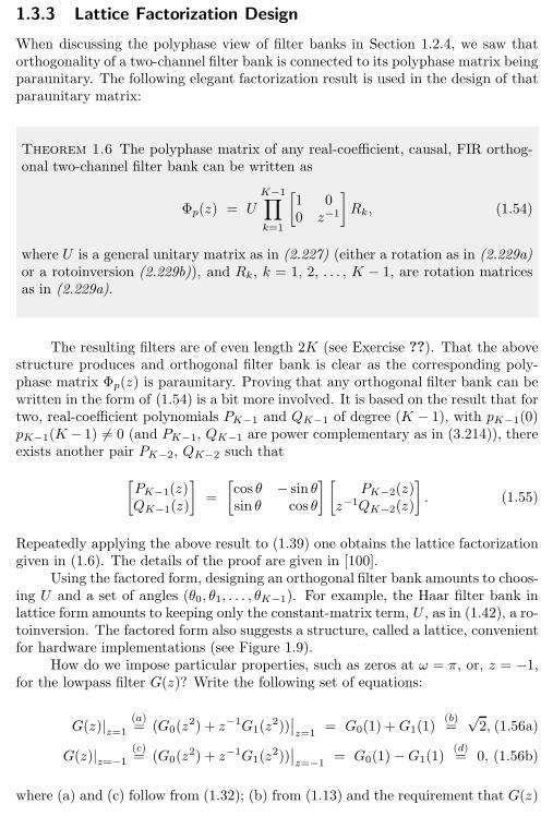
When discussing the polyphase view of filter banks in Section 1.2.4, we saw thatorthogonality of a two-channel filter bank is connected to its polyphase matrix beingparaunitary. The following elegant factorization result is used in the design of thatparaunitary matrix:
Theorem 1.6 The polyphase matrix of any real-coefficient, causal, FIR orthog-onal two-channel filter bank can be written as
Φp(z) = UK−1∏
k=1
[1 00 z−1
]Rk, (1.54)
where U is a general unitary matrix as in (2.227) (either a rotation as in (2.229a)or a rotoinversion (2.229b)), and Rk, k = 1, 2, . . . , K − 1, are rotation matricesas in (2.229a).
The resulting filters are of even length 2K (see Exercise ??). That the abovestructure produces and orthogonal filter bank is clear as the corresponding poly-phase matrix Φp(z) is paraunitary. Proving that any orthogonal filter bank can bewritten in the form of (1.54) is a bit more involved. It is based on the result that fortwo, real-coefficient polynomials PK−1 and QK−1 of degree (K − 1), with pK−1(0)pK−1(K − 1) 6= 0 (and PK−1, QK−1 are power complementary as in (3.214)), thereexists another pair PK−2, QK−2 such that
[PK−1(z)QK−1(z)
]=
[cos θ − sin θsin θ cos θ
] [PK−2(z)
z−1QK−2(z)
]. (1.55)
Repeatedly applying the above result to (1.39) one obtains the lattice factorizationgiven in (1.6). The details of the proof are given in [100].
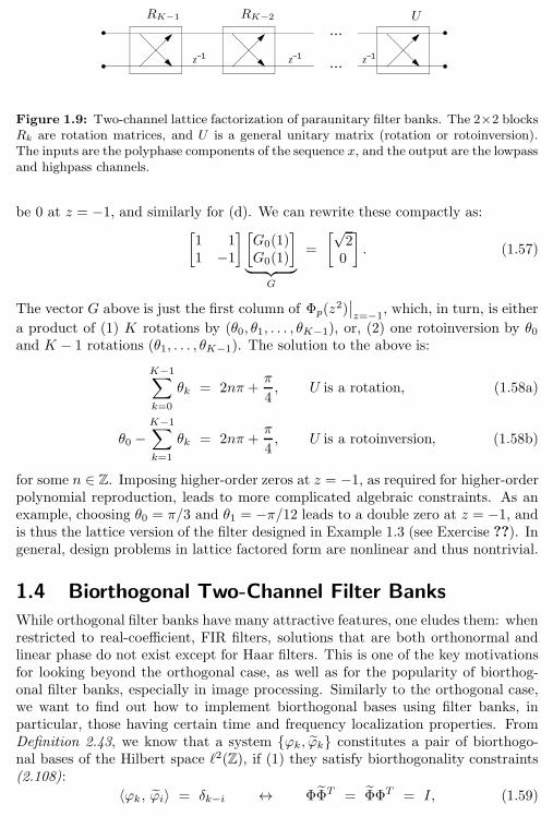
Using the factored form, designing an orthogonal filter bank amounts to choos-ing U and a set of angles (θ0, θ1, . . . , θK−1). For example, the Haar filter bank inlattice form amounts to keeping only the constant-matrix term, U , as in (1.42), a ro-toinversion. The factored form also suggests a structure, called a lattice, convenientfor hardware implementations (see Figure 1.9).
How do we impose particular properties, such as zeros at ω = π, or, z = −1,for the lowpass filter G(z)? Write the following set of equations:
G(z)|z=1
(a)= (G0(z
2) + z−1G1(z2))∣∣z=1
= G0(1) +G1(1)(b)=√2, (1.56a)
G(z)|z=−1
(c)= (G0(z
2) + z−1G1(z2))∣∣z=−1
= G0(1)−G1(1)(d)= 0, (1.56b)
where (a) and (c) follow from (1.32); (b) from (1.13) and the requirement that G(z)
26 Chapter 1. Filter Banks: Building Blocks of Time-Frequency Expansions
z−1z−1z−1
• • •
• • •
figA.1.0FIGURE 3.5
RK−1 RK−2 U
Figure 1.9: Two-channel lattice factorization of paraunitary filter banks. The 2×2 blocksRk are rotation matrices, and U is a general unitary matrix (rotation or rotoinversion).The inputs are the polyphase components of the sequence x, and the output are the lowpassand highpass channels.
be 0 at z = −1, and similarly for (d). We can rewrite these compactly as:[1 11 −1
] [G0(1)G0(1)
]
︸ ︷︷ ︸G
=
[√20
]. (1.57)
The vector G above is just the first column of Φp(z2)∣∣z=−1
, which, in turn, is either
a product of (1) K rotations by (θ0, θ1, . . . , θK−1), or, (2) one rotoinversion by θ0and K − 1 rotations (θ1, . . . , θK−1). The solution to the above is:
K−1∑
k=0
θk = 2nπ +π
4, U is a rotation, (1.58a)
θ0 −K−1∑
k=1
θk = 2nπ +π
4, U is a rotoinversion, (1.58b)
for some n ∈ Z. Imposing higher-order zeros at z = −1, as required for higher-orderpolynomial reproduction, leads to more complicated algebraic constraints. As anexample, choosing θ0 = π/3 and θ1 = −π/12 leads to a double zero at z = −1, andis thus the lattice version of the filter designed in Example 1.3 (see Exercise ??). Ingeneral, design problems in lattice factored form are nonlinear and thus nontrivial.
1.4 Biorthogonal Two-Channel Filter Banks
While orthogonal filter banks have many attractive features, one eludes them: whenrestricted to real-coefficient, FIR filters, solutions that are both orthonormal andlinear phase do not exist except for Haar filters. This is one of the key motivationsfor looking beyond the orthogonal case, as well as for the popularity of biorthog-onal filter banks, especially in image processing. Similarly to the orthogonal case,we want to find out how to implement biorthogonal bases using filter banks, inparticular, those having certain time and frequency localization properties. FromDefinition 2.43, we know that a system ϕk, ϕk constitutes a pair of biorthogo-nal bases of the Hilbert space ℓ2(Z), if (1) they satisfy biorthogonality constraints(2.108):
〈ϕk, ϕi〉 = δk−i ↔ ΦΦT = ΦΦT = I, (1.59)
1.4. Biorthogonal Two-Channel Filter Banks 27
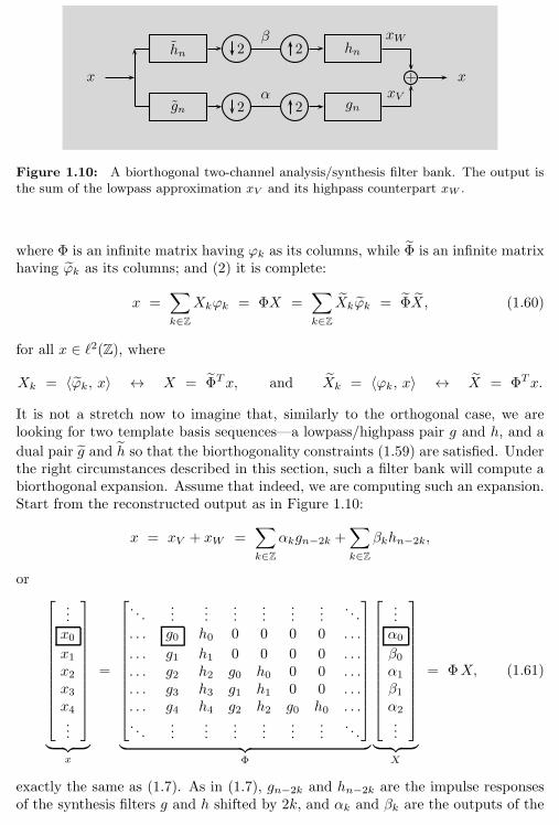
x
hn 2β
2 hn
gn 2α
2 gn
xW
xV+ x
Figure 1.10: A biorthogonal two-channel analysis/synthesis filter bank. The output isthe sum of the lowpass approximation xV and its highpass counterpart xW .
where Φ is an infinite matrix having ϕk as its columns, while Φ is an infinite matrixhaving ϕk as its columns; and (2) it is complete:
x =∑
k∈Z
Xkϕk = ΦX =∑
k∈Z
Xkϕk = ΦX, (1.60)
for all x ∈ ℓ2(Z), where
Xk = 〈ϕk, x〉 ↔ X = ΦTx, and Xk = 〈ϕk, x〉 ↔ X = ΦTx.
It is not a stretch now to imagine that, similarly to the orthogonal case, we arelooking for two template basis sequences—a lowpass/highpass pair g and h, and a
dual pair g and h so that the biorthogonality constraints (1.59) are satisfied. Underthe right circumstances described in this section, such a filter bank will compute abiorthogonal expansion. Assume that indeed, we are computing such an expansion.Start from the reconstructed output as in Figure 1.10:
x = xV + xW =∑
k∈Z
αkgn−2k +∑
k∈Z
βkhn−2k,
or
...x0x1x2x3x4...
︸ ︷︷ ︸x
=
. . ....
......
......
.... . .
. . . g0 h0 0 0 0 0 . . .
. . . g1 h1 0 0 0 0 . . .
. . . g2 h2 g0 h0 0 0 . . .
. . . g3 h3 g1 h1 0 0 . . .
. . . g4 h4 g2 h2 g0 h0 . . .
. . ....
......
......
.... . .
︸ ︷︷ ︸Φ
...α0
β0α1
β1α2
...
︸ ︷︷ ︸X
= ΦX, (1.61)
exactly the same as (1.7). As in (1.7), gn−2k and hn−2k are the impulse responsesof the synthesis filters g and h shifted by 2k, and αk and βk are the outputs of the
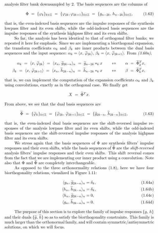
28 Chapter 1. Filter Banks: Building Blocks of Time-Frequency Expansions
analysis filter bank downsampled by 2. The basis sequences are the columns of
Φ = ϕkk∈Z = ϕ2k, ϕ2k+1k∈Z = gn−2k, hn−2kk∈Z, (1.62)
that is, the even-indexed basis sequences are the impulse responses of the synthesislowpass filter and its even shifts, while the odd-indexed basis sequences are theimpulse responses of the synthesis highpass filter and its even shifts.
So far, the analysis has been identical to that of orthogonal filter banks; werepeated it here for emphasis. Since we are implementing a biorthogonal expansion,the transform coefficients αk and βk are inner products between the dual basissequences and the input sequence: αk = 〈x, ϕ2k〉, βk = 〈x, ϕ2k+1〉. From (3.60a),
αk = 〈x, ϕ2k〉 = 〈xn, g2k−n〉n = gn−2k ∗k x ↔ α = ΦTgx,
βk = 〈x, ϕ2k+1〉 = 〈xn, h2k−n〉n = hn−2k ∗k x ↔ β = ΦThx,
that is, we can implement the computation of the expansion coefficients αk and βkusing convolutions, exactly as in the orthogonal case. We finally get
X = ΦTx.
From above, we see that the dual basis sequences are
Φ = ϕkk∈Z = ϕ2k, ϕ2k+1k∈Z = g2k−n, h2k−nk∈Z, (1.63)
that is, the even-indexed dual basis sequences are the shift-reversed impulse re-sponses of the analysis lowpass filter and its even shifts, while the odd-indexedbasis sequences are the shift-reversed impulse responses of the analysis highpassfilter and its even shifts.
We stress again that the basis sequences of Φ are synthesis filters’ impulseresponses and their even shifts, while the basis sequences of Φ are the shift-reversedanalysis filters’ impulse responses and their even shifts. This shift reversal comesfrom the fact that we are implementing our inner product using a convolution. Notealso that Φ and Φ are completely interchangeable.
As opposed to the three orthonormality relations (1.8), here we have fourbiorthogonality relations, visualized in Figure 1.11:
〈gn, g2k−n〉n = δk, (1.64a)
〈hn, h2k−n〉n = δk, (1.64b)
〈hn, g2k−n〉n = 0, (1.64c)
〈gn, h2k−n〉n = 0. (1.64d)
The purpose of this section is to explore the family of impulse responses g, hand their duals g, h so as to satisfy the biorthogonality constraints. This family ismuch larger than the orthonormal family, and will contain symmetric/antisymmetricsolutions, on which we will focus.
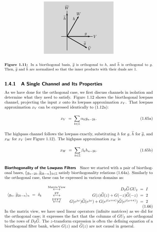
1.4. Biorthogonal Two-Channel Filter Banks 29
Wh
V
g
Vg
W
h
Figure 1.11: In a biorthogonal basis, g is orthogonal to h, and h is orthogonal to g.Then, g and h are normalized so that the inner products with their duals are 1.
1.4.1 A Single Channel and Its Properties
As we have done for the orthogonal case, we first discuss channels in isolation anddetermine what they need to satisfy. Figure 1.12 shows the biorthogonal lowpasschannel, projecting the input x onto its lowpass approximation xV . That lowpassapproximation xV can be expressed identically to (1.12a):
xV =∑
k∈Z
αkgn−2k. (1.65a)
The highpass channel follows the lowpass exactly, substituting h for g, h for g, andxW for xV (see Figure 1.12). The highpass approximation xW is
xW =∑
k∈Z
βkhn−2k. (1.65b)
Biorthogonality of the Lowpass Filters Since we started with a pair of biorthog-onal bases, gn−2k, g2k−nk∈Z satisfy biorthogonality relations (1.64a). Similarly tothe orthogonal case, these can be expressed in various domains as:
〈gn, g2k−n〉n = δk
MatrixView←→ D2GGU2 = IZT←→ G(z)G(z) +G(−z)G(−z) = 2
DTFT←→ G(ejω)G(ejω) +G(ej(ω+π))G(ej(ω+π)) = 2(1.66)
In the matrix view, we have used linear operators (infinite matrices) as we did forthe orthogonal case; it expresses the fact that the columns of GU2 are orthogonalto the rows of D2G. The z-transform expression is often the defining equation of abiorthogonal filter bank, where G(z) and G(z) are not causal in general.
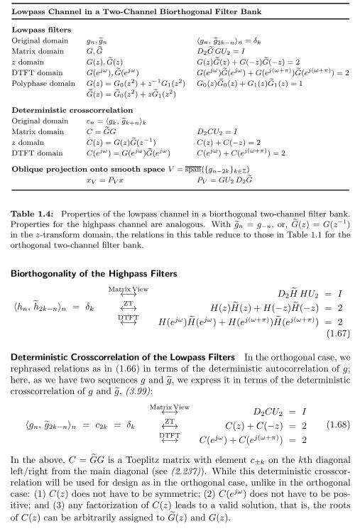
30 Chapter 1. Filter Banks: Building Blocks of Time-Frequency Expansions
Lowpass Channel in a Two-Channel Biorthogonal Filter Bank
Lowpass filters
Original domain gn, gn 〈gn, g2k−n〉n = δkMatrix domain G, G D2GGU2 = I
z domain G(z), G(z) G(z)G(z) +G(−z)G(−z) = 2
DTFT domain G(ejω), G(ejω) G(ejω)G(ejω) +G(ej(ω+π))G(ej(ω+π)) = 2
Polyphase domain G(z) = G0(z2) + z−1G1(z
2) G0(z)G0(z) +G1(z)G1(z) = 1
G(z) = G0(z2) + zG1(z
2)
Deterministic crosscorrelation
Original domain cn = 〈gk, gk+n〉kMatrix domain C = GG D2CU2 = I
z domain C(z) = G(z)G(z−1) C(z) + C(−z) = 2
DTFT domain C(ejω) = G(ejω)G(ejω) C(ejω) + C(ej(ω+π)) = 2
Oblique projection onto smooth space V = span(gn−2kk∈Z)
xV = PV x PV = GU2D2G
Table 1.4: Properties of the lowpass channel in a biorthogonal two-channel filter bank.Properties for the highpass channel are analogous. With gn = g−n, or, G(z) = G(z−1)in the z-transform domain, the relations in this table reduce to those in Table 1.1 for theorthogonal two-channel filter bank.
Biorthogonality of the Highpass Filters
〈hn, h2k−n〉n = δk
MatrixView←→ D2H HU2 = IZT←→ H(z)H(z) +H(−z)H(−z) = 2
DTFT←→ H(ejω)H(ejω) +H(ej(ω+π))H(ej(ω+π)) = 2(1.67)
Deterministic Crosscorrelation of the Lowpass Filters In the orthogonal case, werephrased relations as in (1.66) in terms of the deterministic autocorrelation of g;here, as we have two sequences g and g, we express it in terms of the deterministiccrosscorrelation of g and g, (3.99):
〈gn, g2k−n〉n = c2k = δk
MatrixView←→ D2CU2 = IZT←→ C(z) + C(−z) = 2
DTFT←→ C(ejω) + C(ej(ω+π)) = 2
(1.68)
In the above, C = GG is a Toeplitz matrix with element c±k on the kth diagonalleft/right from the main diagonal (see (2.237)). While this deterministic crosscor-relation will be used for design as in the orthogonal case, unlike in the orthogonalcase: (1) C(z) does not have to be symmetric; (2) C(ejω) does not have to be pos-itive; and (3) any factorization of C(z) leads to a valid solution, that is, the roots
of C(z) can be arbitrarily assigned to G(z) and G(z).
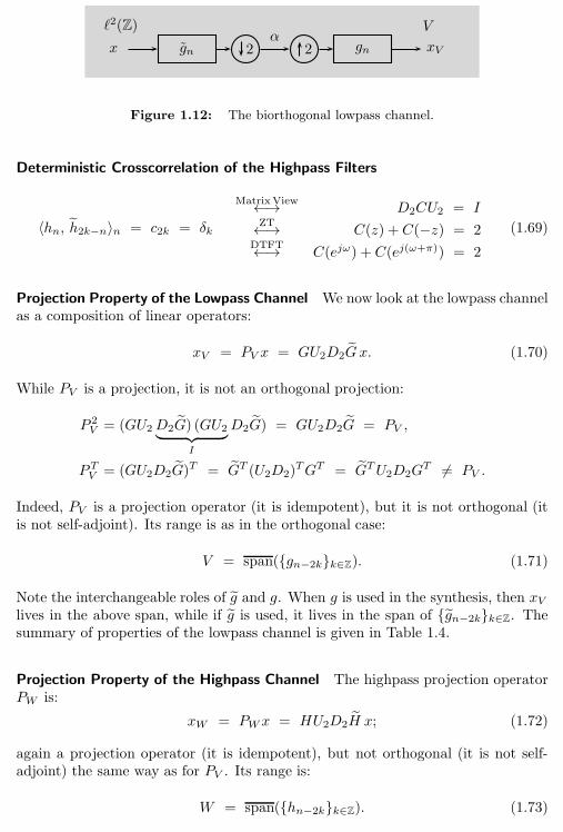
1.4. Biorthogonal Two-Channel Filter Banks 31
x
ℓ2(Z)
gn 2α
2 gn
V
xV
Figure 1.12: The biorthogonal lowpass channel.
Deterministic Crosscorrelation of the Highpass Filters
〈hn, h2k−n〉n = c2k = δk
MatrixView←→ D2CU2 = IZT←→ C(z) + C(−z) = 2
DTFT←→ C(ejω) + C(ej(ω+π)) = 2
(1.69)
Projection Property of the Lowpass Channel We now look at the lowpass channelas a composition of linear operators:
xV = PV x = GU2D2G x. (1.70)
While PV is a projection, it is not an orthogonal projection:
P 2V= (GU2D2G) (GU2︸ ︷︷ ︸
I
D2G) = GU2D2G = PV ,
PTV
= (GU2D2G)T = GT (U2D2)
TGT = GTU2D2GT 6= PV .
Indeed, PV is a projection operator (it is idempotent), but it is not orthogonal (itis not self-adjoint). Its range is as in the orthogonal case:
V = span(gn−2kk∈Z). (1.71)
Note the interchangeable roles of g and g. When g is used in the synthesis, then xVlives in the above span, while if g is used, it lives in the span of gn−2kk∈Z. Thesummary of properties of the lowpass channel is given in Table 1.4.
Projection Property of the Highpass Channel The highpass projection operatorPW is:
xW = PWx = HU2D2H x; (1.72)
again a projection operator (it is idempotent), but not orthogonal (it is not self-adjoint) the same way as for PV . Its range is:
W = span(hn−2kk∈Z). (1.73)
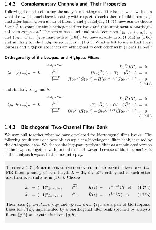
32 Chapter 1. Filter Banks: Building Blocks of Time-Frequency Expansions
1.4.2 Complementary Channels and Their Properties
Following the path set during the analysis of orthogonal filter banks, we now discusswhat the two channels have to satisfy with respect to each other to build a biorthog-onal filter bank. Given a pair of filters g and g satisfying (1.66), how can we choose
h and h to complete the biorthogonal filter bank and thus implement a biorthogo-nal basis expansion? The sets of basis and dual basis sequences gn−2k, hn−2kk∈Z
and g2k−n, h2k−nk∈Z must satisfy (1.64). We have already used (1.64a) in (1.66)and similarly for the highpass sequences in (1.67). What is left to use is that theselowpass and highpass sequences are orthogonal to each other as in (1.64c)–(1.64d):
Orthogonality of the Lowpass and Highpass Filters
〈hn, g2k−n〉n = 0
MatrixView←→ D2GHU2 = 0ZT←→ H(z)G(z) +H(−z)G(−z) = 0
DTFT←→ H(ejω)G(ejω) +H(ej(ω+π))G(ej(ω+π)) = 0(1.74a)
and similarly for g and h:
〈gn, h2k−n〉n = 0
MatrixView←→ D2H GU2 = 0ZT←→ G(z)H(z) +G(−z)H(−z) = 0
DTFT←→ G(ejω)H(ejω) +G(ej(ω+π))H(ej(ω+π)) = 0(1.74b)
1.4.3 Biorthogonal Two-Channel Filter Bank
We now pull together what we have developed for biorthogonal filter banks. Thefollowing result gives one possible example of a biorthogonal filter bank, inspired bythe orthogonal case. We choose the highpass synthesis filter as a modulated versionof the lowpass, together with an odd shift. However, because of biorthogonality, itis the analysis lowpass that comes into play.
Theorem 1.7 (Biorthogonal two-channel filter bank) Given are twoFIR filters g and g of even length L = 2ℓ, ℓ ∈ Z+, orthogonal to each otherand their even shifts as in (1.66). Choose
hn = (−1)ngn−2ℓ+1ZT←→ H(z) = −z−L+1G(−z) (1.75a)
hn = (−1)ngn+2ℓ−1ZT←→ H(z) = −zL−1G(−z) (1.75b)
Then, sets gn−2k, hn−2kk∈Z and g2k−n, h2k−nk∈Z are a pair of biorthogonalbases for ℓ2(Z), implemented by a biorthogonal filter bank specified by analysis
filters g, h and synthesis filters g, h.
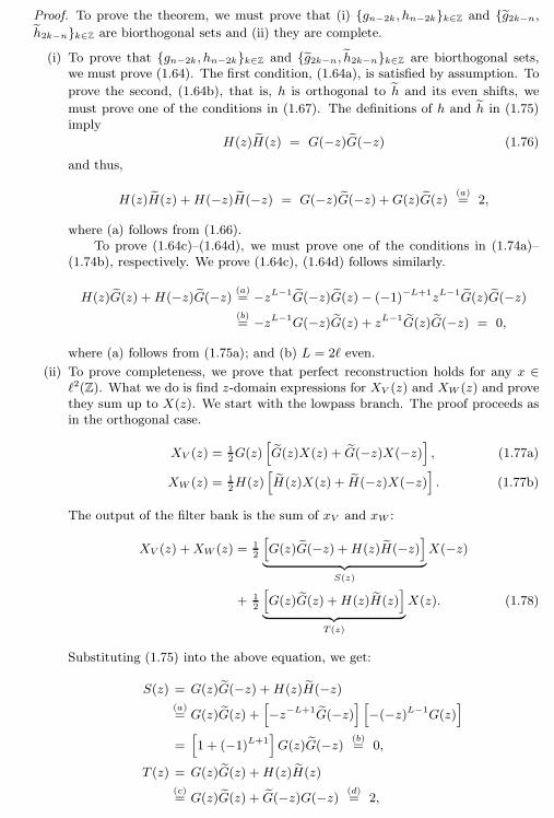
1.4. Biorthogonal Two-Channel Filter Banks 33
Proof. To prove the theorem, we must prove that (i) gn−2k, hn−2kk∈Z and g2k−n,h2k−nk∈Z are biorthogonal sets and (ii) they are complete.
(i) To prove that gn−2k, hn−2kk∈Z and g2k−n, h2k−nk∈Z are biorthogonal sets,we must prove (1.64). The first condition, (1.64a), is satisfied by assumption. To
prove the second, (1.64b), that is, h is orthogonal to h and its even shifts, we
must prove one of the conditions in (1.67). The definitions of h and h in (1.75)imply
H(z)H(z) = G(−z)G(−z) (1.76)
and thus,
H(z)H(z) +H(−z)H(−z) = G(−z)G(−z) +G(z)G(z)(a)= 2,
where (a) follows from (1.66).To prove (1.64c)–(1.64d), we must prove one of the conditions in (1.74a)–
(1.74b), respectively. We prove (1.64c), (1.64d) follows similarly.
H(z)G(z) +H(−z)G(−z) (a)= −zL−1G(−z)G(z)− (−1)−L+1zL−1G(z)G(−z)(b)= −zL−1G(−z)G(z) + zL−1G(z)G(−z) = 0,
where (a) follows from (1.75a); and (b) L = 2ℓ even.
(ii) To prove completeness, we prove that perfect reconstruction holds for any x ∈ℓ2(Z). What we do is find z-domain expressions for XV (z) and XW (z) and provethey sum up to X(z). We start with the lowpass branch. The proof proceeds asin the orthogonal case.
XV (z) =12G(z)
[G(z)X(z) + G(−z)X(−z)
], (1.77a)
XW (z) = 12H(z)
[H(z)X(z) + H(−z)X(−z)
]. (1.77b)
The output of the filter bank is the sum of xV and xW :
XV (z) +XW (z) = 12
[G(z)G(−z) +H(z)H(−z)
]
︸ ︷︷ ︸S(z)
X(−z)
+ 12
[G(z)G(z) +H(z)H(z)
]
︸ ︷︷ ︸T (z)
X(z). (1.78)
Substituting (1.75) into the above equation, we get:
S(z) = G(z)G(−z) +H(z)H(−z)(a)= G(z)G(z) +
[−z−L+1G(−z)
] [−(−z)L−1G(z)
]
=[1 + (−1)L+1
]G(z)G(−z) (b)
= 0,
T (z) = G(z)G(z) +H(z)H(z)
(c)= G(z)G(z) + G(−z)G(−z) (d)
= 2,
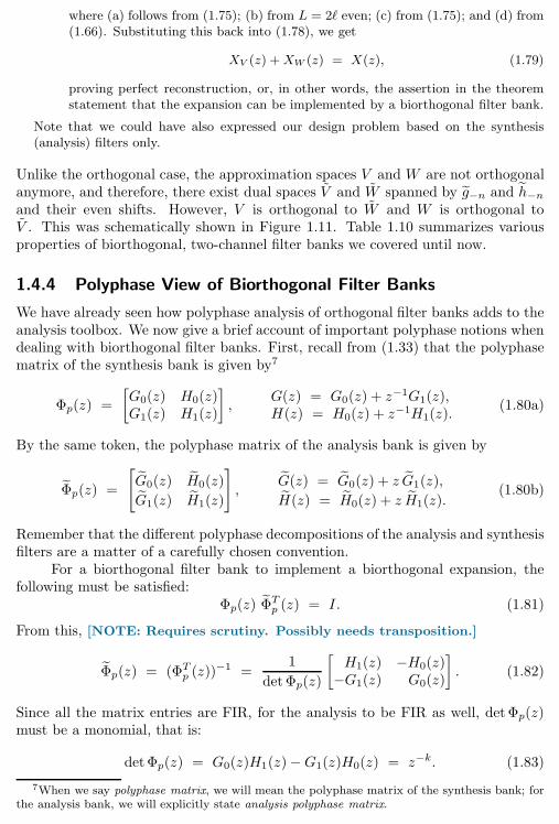
34 Chapter 1. Filter Banks: Building Blocks of Time-Frequency Expansions
where (a) follows from (1.75); (b) from L = 2ℓ even; (c) from (1.75); and (d) from(1.66). Substituting this back into (1.78), we get
XV (z) +XW (z) = X(z), (1.79)
proving perfect reconstruction, or, in other words, the assertion in the theoremstatement that the expansion can be implemented by a biorthogonal filter bank.
Note that we could have also expressed our design problem based on the synthesis(analysis) filters only.
Unlike the orthogonal case, the approximation spaces V and W are not orthogonalanymore, and therefore, there exist dual spaces V and W spanned by g−n and h−nand their even shifts. However, V is orthogonal to W and W is orthogonal toV . This was schematically shown in Figure 1.11. Table 1.10 summarizes variousproperties of biorthogonal, two-channel filter banks we covered until now.
1.4.4 Polyphase View of Biorthogonal Filter Banks
We have already seen how polyphase analysis of orthogonal filter banks adds to theanalysis toolbox. We now give a brief account of important polyphase notions whendealing with biorthogonal filter banks. First, recall from (1.33) that the polyphasematrix of the synthesis bank is given by7
Φp(z) =
[G0(z) H0(z)G1(z) H1(z)
],
G(z) = G0(z) + z−1G1(z),H(z) = H0(z) + z−1H1(z).
(1.80a)
By the same token, the polyphase matrix of the analysis bank is given by
Φp(z) =
[G0(z) H0(z)
G1(z) H1(z)
],
G(z) = G0(z) + z G1(z),
H(z) = H0(z) + z H1(z).(1.80b)
Remember that the different polyphase decompositions of the analysis and synthesisfilters are a matter of a carefully chosen convention.
For a biorthogonal filter bank to implement a biorthogonal expansion, thefollowing must be satisfied:
Φp(z) ΦT
p(z) = I. (1.81)
From this, [NOTE: Requires scrutiny. Possibly needs transposition.]
Φp(z) = (ΦTp(z))−1 =
1
det Φp(z)
[H1(z) −H0(z)−G1(z) G0(z)
]. (1.82)
Since all the matrix entries are FIR, for the analysis to be FIR as well, detΦp(z)must be a monomial, that is:
detΦp(z) = G0(z)H1(z)−G1(z)H0(z) = z−k. (1.83)
7When we say polyphase matrix, we will mean the polyphase matrix of the synthesis bank; forthe analysis bank, we will explicitly state analysis polyphase matrix.
1.4. Biorthogonal Two-Channel Filter Banks 35
In the above, we have implicitly assumed that Φp(z) was invertible, that is, itscolumns are linearly independent. This can be rephrased in filter bank terms bystating when, given G(z), it is possible to find H(z) such that it leads to a per-fect reconstruction biorthogonal filter bank. Such a filter H(z) will be called acomplementary filter.
Theorem 1.8 (Complementary filters) Given a causal FIR filter G(z),there exists a complementary FIR filter H(z), if and only if the polyphase com-ponents of G(z) are coprime (except for possible zeros at z =∞).
Proof. We just saw that a necessary and sufficient condition for perfect FIR recon-struction is that det(Φp(z)) be a monomial. Thus, coprimeness is obviously necessary,since if there were a common factor between G0(z) and G1(z), it would show up in thedeterminant.
Sufficiency follows from the Bezout’s identity (3.290) that says that given twocoprime polynomials a(z) and b(z), the equation a(z)p(z) + b(z)q(z) = c(z) has asolution p(z), q(z). Fixing a(z) = G0(z), b(z) = G1(z) and c(z) = z−k, we see thatBezout’s identity is equal to (1.83), and thus guarantees a solution p(z) = H0(z) andq(z) = H1(z), that is, a complementary filter H(z).
Note that the coprimeness of G0(z) and G1(z) is equivalent to G(z) not having anyzero pairs z0,−z0. This can be used to prove that the binomial filter G(z) =(1 + z−1)N always has a complementary filter (see Exercise ??).
The counterpart to Theorem 1.3 and Corollary 1.4 for orthogonal filter banksare the following theorem and corollary for the biorthogonal ones (we state thesewithout proof):
Theorem 1.9 (Positive definite matrix and biorthogonal basis) Givena filter bank implementing a biorthogonal basis for ℓ2(Z) and its associatedpolyphase matrix Φp(e
jω), then Φp(ejω)ΦT
p(e−jω) is positive definite.
Corollary 1.10 (Filtered deterministic autocorrelation matrix is positive semidefinite)Given is a 2× 2 polyphase matrix Φp(e
jω) such that Φp(ejω)ΦT
p(e−jω). Then the
filtered deterministic autocorrelation matrix, Ap,α(ejω), is positive semidefinite.
1.4.5 Linear-Phase Two-Channel Filter Banks
We started this section by saying that one of the reasons we go through the troubleof analyzing and constructing two-channel biorthogonal filter banks is because they

36 Chapter 1. Filter Banks: Building Blocks of Time-Frequency Expansions
allow us to obtain real-coefficient FIR filters with linear phase.8 Thus, we now dojust that: we build perfect reconstruction filter banks where all the filters involvedare linear phase. Linear-phase filters were defined in (3.107).
As was true for orthogonal filters, not all lengths of filters are possible if wewant to have a linear-phase filter bank. This is summarized in the following theorem,the proof of which is left as Exercise ??:
Theorem 1.11 In a two-channel, perfect reconstruction filter bank where all fil-ters are linear phase, the synthesis filters have one of the following forms:
(i) Both filters are odd-length symmetric, the lengths differing by an odd mul-tiple of 2.
(ii) One filter is symmetric and the other is antisymmetric; both lengths areeven, and are equal or differ by an even multiple of 2.
(iii) One filter is of odd length, the other one of even length; both have all zeroson the unit circle. Either both filters are symmetric, or one is symmetricand the other one is antisymmetric.
Our next task is to show that indeed, it is not possible to have an orthogonalfilter bank with linear-phase filters if we restrict ourselves to the two-channel, FIR,real-coefficient case:
Theorem 1.12 The only two-channel perfect reconstruction orthogonal filterbank with real-coefficient FIR linear-phase filters is the Haar filter bank.
Proof. In orthogonal filter banks, (1.40)–(1.41) hold, and the filters are of even length.Therefore, following Theorem 1.11, one filter is symmetric and the other antisymmetric.Take the symmetric one, G(z) for example,
G(z)(a)= G0(z
2) + z−1G1(z2)
(b)= z−L+1G(z−1)
(c)= z−L+1(G0(z
−2) + zG1(z−2))
= z−L+2G1(z−2) + z−1(z−L+2G0(z
−2)),
where (a) and (c) follow from (1.32), and (b) from (3.153). This further means thatfor the polyphase components, the following hold:
G0(z) = z−L/2+1G1(z−1), G1(z) = z−L/2+1G0(z
−1). (1.84)
Substituting (1.84) into (1.40) we obtain
G0(z) G0(z−1) = 1
2.
8If we allow filters to have complex-valued coefficients or if we lift the restriction of two channels,linear phase and orthogonality can be satisfied simultaneously.
1.5. Design of Biorthogonal Two-Channel Filter Banks 37
The only FIR, real-coefficient polynomial satisfying the above is
G0(z) = 1√2z−m.
Performing a similar analysis for G1(z), we get that G1(z) = (1/√2)z−k, and
G(z) = 1√2(z−2ℓ + z−2k−1), H(z) = G(−z),
yielding Haar filters (m = k = 0) or trivial variations thereof.
While the outstanding features of the Haar filters make it a very special solution,Theorem 1.12 is a fundamentally negative result as the Haar filters have poor fre-quency localization and no polynomial reproduction capability.
1.5 Design of Biorthogonal Two-Channel FilterBanks
Given that biorthogonal filters are less constrained than their orthogonal counter-parts, the design space is much more open. In both cases, one factors a Laurentpolynomial9 C(z) satisfying C(z)+C(−z) = 2 as in (1.68). In the orthogonal case,C(z) was a deterministic autocorrelation, while in the biorthogonal case, it is a de-terministic crosscorrelation and thus more general. In addition, the orthogonal caserequires spectral factorization (square root), while in the biorthogonal case, any fac-torization will do. While the factorization method is not the only approach, it is themost common. Other approaches include the complementary filter design methodand the lifting design method. In the former, a desired filter is complemented soas to obtain a perfect reconstruction filter bank. In the latter, a structure akinto a lattice is used to guarantee perfect reconstruction as well as other desirableproperties.
1.5.1 Factorization Design
From (1.66)–(1.68), C(z) satisfying C(z) + C(−z) = 2 can be factored into
C(z) = G(z)G(z),
where G(z) is the synthesis and G(z) the analysis lowpass filter (or vice-versa, sincethe roles are dual). The most common designs use the same C(z) as those usedin orthogonal filter banks, for example, those with a maximum number of zeros atz = −1, performing the factorization so that the resulting filters have linear phase.
Example 1.4 (Biorthogonal filter bank with linear-phase filters) Wereconsider Example 1.3, in particular C(z) given by
C(z) =(1 + z−1
)2(1 + z)2
1
4
(−1
4z−1 + 1− 1
4z
),
9A Laurent polynomial is a polynomial with both positive and negative powers, see Ap-pendix 3.B.1.
38 Chapter 1. Filter Banks: Building Blocks of Time-Frequency Expansions
which satisfies C(z) + C(−z) = 2 by construction. This also means it satisfies
(1.66) for any factorization of C(z) into G(z)G(z). Note that we can add factorsz or z−1 in one filter, as long as we cancel it in the other; this is useful forobtaining purely causal/anticausal solutions.
One possible factorization is
G(z) = z−1(1 + z−1
)2(1 + z) =
(1 + z−1
)3= 1 + 3z−1 + 3z−2 + z−3,
G(z) = z(1 + z)1
4
(−1
4z−1 + 1− 1
4z
)=
1
16
(−1 + 3z + 3z2 − z3
).
The other filters follow from (1.75), with L = 2ℓ = 4:
H(z) = −z−3 1
16
(−1− 3z + 3z2 + z3
)=
1
16
(−1− 3z−1 + 3z−2 + z−3
),
H(z) = −z3(1− 3z−1 + 3z−2 − z−3
)= 1− 3z + 3z2 − z3.
The lowpass filters are both symmetric, while the highpass ones are antisymmet-ric. As H(z) has three zero moments, G(z) can reproduce polynomials up todegree 2, since such sequences go through the lowpass channel only.
Another possible factorization is
G(z) =(1 + z−1
)2(1 + z)2 = z−2 + 4z−1 + 6 + 4z + z2,
G(z) =1
4
(−1
4z−1 + 1− 1
4z
)=
1
16
(−z−1 + 4− z
),
where both lowpass filters are symmetric and zero phase. The highpass filtersare (with L = 0):
H(z) = − 1
16z(z−1 + 4 + z
),
H(z) = −z−1(z−2 − 4z−1 + 6− 4z + z2
),
which are also symmetric, but with a phase delay of ±1 sample.
The zeros at z = −1 in the synthesis lowpass filter become, following (1.75b),zeros at z = 1 in the analysis highpass filter. Therefore, many popular biorthogonalfilters come from symmetric factorizations of C(z) with a maximum number of zerosat z = −1.
Example 1.5 (Design of the 9/7 filter pair) The next higher-degreeC(z)with a maximum number of zeros at z = −1 is of the form
C(z) = 2−8 (1 + z)3 (
1 + z−1)3 (
3z2 − 18z + 38− 18z−1 + 3z−2).
One possible factorization yields the so-called Daubechies 9/7 filter pair (seeTable 1.5). These filters have odd length and even symmetry, and are part of theJPEG 2000 image compression standard.
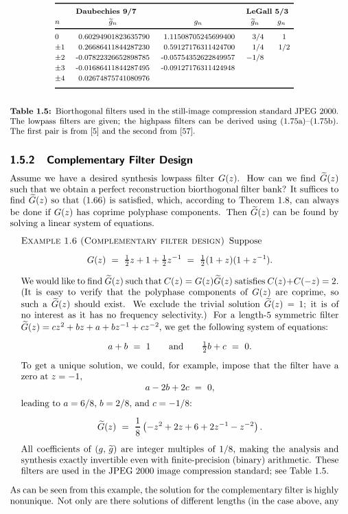
1.5. Design of Biorthogonal Two-Channel Filter Banks 39
Daubechies 9/7 LeGall 5/3
n gn gn gn gn
0 0.60294901823635790 1.11508705245699400 3/4 1
±1 0.26686411844287230 0.59127176311424700 1/4 1/2
±2 -0.07822326652898785 -0.05754352622849957 −1/8
±3 -0.01686411844287495 -0.09127176311424948
±4 0.02674875741080976
Table 1.5: Biorthogonal filters used in the still-image compression standard JPEG 2000.The lowpass filters are given; the highpass filters can be derived using (1.75a)–(1.75b).The first pair is from [5] and the second from [57].
1.5.2 Complementary Filter Design
Assume we have a desired synthesis lowpass filter G(z). How can we find G(z)such that we obtain a perfect reconstruction biorthogonal filter bank? It suffices tofind G(z) so that (1.66) is satisfied, which, according to Theorem 1.8, can always
be done if G(z) has coprime polyphase components. Then G(z) can be found bysolving a linear system of equations.
Example 1.6 (Complementary filter design) Suppose
G(z) = 12z + 1 + 1
2z−1 = 1
2 (1 + z)(1 + z−1).
We would like to find G(z) such that C(z) = G(z)G(z) satisfies C(z)+C(−z) = 2.(It is easy to verify that the polyphase components of G(z) are coprime, so
such a G(z) should exist. We exclude the trivial solution G(z) = 1; it is ofno interest as it has no frequency selectivity.) For a length-5 symmetric filter
G(z) = cz2 + bz + a+ bz−1 + cz−2, we get the following system of equations:
a+ b = 1 and 12b+ c = 0.
To get a unique solution, we could, for example, impose that the filter have azero at z = −1,
a− 2b+ 2c = 0,
leading to a = 6/8, b = 2/8, and c = −1/8:
G(z) =1
8
(−z2 + 2z + 6 + 2z−1 − z−2
).
All coefficients of (g, g) are integer multiples of 1/8, making the analysis andsynthesis exactly invertible even with finite-precision (binary) arithmetic. Thesefilters are used in the JPEG 2000 image compression standard; see Table 1.5.
As can be seen from this example, the solution for the complementary filter is highlynonunique. Not only are there solutions of different lengths (in the case above, any
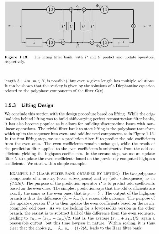
40 Chapter 1. Filter Banks: Building Blocks of Time-Frequency Expansions
x
z 2
2
P
+−
U
+
β
α+−
U
+
P
Φg
Φh2
2
z−1
+ x
Figure 1.13: The lifting filter bank, with P and U predict and update operators,respectively.
length 3 + 4m, m ∈ N, is possible), but even a given length has multiple solutions.It can be shown that this variety is given by the solutions of a Diophantine equationrelated to the polyphase components of the filter G(z).
1.5.3 Lifting Design
We conclude this section with the design procedure based on lifting. While the orig-inal idea behind lifting was to build shift-varying perfect reconstruction filter banks,it has also become popular as it allows for building discrete-time bases with non-linear operations. The trivial filter bank to start lifting is the polyphase transformwhich splits the sequence into even- and odd-indexed components as in Figure 1.13.In the first lifting step, we use a prediction filter P to predict the odd coefficientsfrom the even ones. The even coefficients remain unchanged, while the result ofthe prediction filter applied to the even coefficients is subtracted from the odd co-efficients yielding the highpass coefficients. In the second step, we use an updatefilter U to update the even coefficients based on the previously computed highpasscoefficients. We start with a simple example.
Example 1.7 (Haar filter bank obtained by lifting) The two polyphasecomponents of x are x0 (even subsequence) and x1 (odd subsequence) as in(3.216). The purpose of the prediction operator P is to predict odd coefficientsbased on the even ones. The simplest prediction says that the odd coefficients areexactly the same as the even ones, that is pn = δn. The output of the highpassbranch is thus the difference (δn − δn−1), a reasonable outcome. The purpose ofthe update operator U is to then update the even coefficients based on the newlycomputed odd ones. As we are looking for a lowpass-like version in the otherbranch, the easiest is to subtract half of this difference from the even sequence,leading to x0,n − (x1,n − x0,n)/2, that is, the average (xo,n + x1,n)/2, again areasonable output, but this time lowpass in nature. Within scaling, it is thusclear that the choice pn = δn, un = (1/2)δn leads to the Haar filter bank.
1.6. Two-Channel Filter Banks with Stochastic Inputs 41
Let us now identify the polyphase matrix Φp(z):
Φg(z) = α(z)− U(z)β(z),
Φh(z) = β(z) + P (z)Φg(z)
= β(z) + P (z)(α(z)− U(z)β(z))
= P (z)α(z) + (1− P (z)U(z))β(z),
which we can write as[Φg(z)Φh(z)
]=
[1 −U(z)
P (z) 1− P (z)U(z)
] [α(z)β(z)
]= Φp(z)
[α(z)β(z)
]. (1.85)
On the analysis side, Φp(z) is:
Φp(z) = (ΦTp(z))−1 =
[1− P (z)U(z) −P (z)
U(z) 1
]. (1.86)
As the det(Φp(z)) = 1, the inverse of Φp(z) does not involve actual inversion, oneof the reasons why this technique is popular. Moreover, we can write Φp as
Φp(z) =
[1 −U(z)
P (z) 1− P (z)U(z)
]=
[1 0
P (z) 1
] [1 −U(z)0 1
], (1.87)
decomposing Φp(z) into a sequence of lower/upper triangular matrices—lifting steps.What we also see is that the inverse of each matrix of the form:
[1 0M 1
]−1
=
[1 0−M 1
]and
[1 M0 1
]−1
=
[1 −M0 1
],
meaning to invert these one needs only reverse the sequence of operations as shownin Figure 1.13. This is why this scheme allows for nonlinear operations; if M isnonlinear, its inversion amounts to simply reversing the sign in the matrix.
1.6 Two-Channel Filter Banks with Stochastic Inputs
Our discussion so far assumed we are dealing with deterministic sequences as in-puts into our filter bank, most often those with finite energy. If the input intoour filter bank is stochastic, then we must use the tools developed in Section 3.8.The periodic shift variance for deterministic systems has its counterpart in wide-sense cyclostationarity. The notions of energy spectral density (3.96) (DTFT ofthe deterministic autocorrelation) and energy (3.98) have their counterparts in thenotions of power spectral density (3.239) (DTFT of the stochastic autocorrelation)and power (3.240). We now briefly discuss the effects of a filter bank on an inputWSS sequence.
Until now, we have seen various ways of characterizing systems with deter-ministic and stochastic inputs, among others via the deterministic and stochasticautocorrelations.
In a single-input single-output system:
42 Chapter 1. Filter Banks: Building Blocks of Time-Frequency Expansions
(i) For a deterministic sequence, its autocorrelation is Hermitian symmetric (see(3.16)) and can be factored as in (3.96), (3.143), that is, it is nonnegative onthe unit circle. It is sometimes called energy spectral density.
(ii) For a WSS sequence, the counterpart to the deterministic autocorrelation isthe power spectral density given in (3.239).
In a multiple-input multiple-output system, such as a filter banks, where themultiple inputs are naturally polyphase components of the input sequence:
(i) For a deterministic sequence, we have a matrix autocorrelation of the vector
of polyphase components[x0 x1
]T
, given by (3.219). In particular, we have
seen it for a the vector of expansion coefficient sequences[α β
]T
in two-channel filter bank earlier in this chapter, in (1.43).
(ii) For a WSS sequence x, we can also look at the matrix of power spectral densi-
ties of the polyphase components[x0 x1
]T
as in (3.247). In what follows, we
analyze that matrix for the vector of expansion coefficient sequences[α β
]T
.
Filter-Bank Optimization Based on Input Statistics The area of optimizing filterbanks based on input statistics is an active one. In particular, principal-componentfilter banks have been shown to be optimal for a wide variety of problems (wegive pointers to the literature on the subject in Further Reading). For example,in parallel to our discussion in Chapter 6 on the use of KLT, it is known that thecoding gain is maximized if the channel sequences are decorrelated, (Φa is diagonal),
and Aα(ejω) ≥ Aβ(e
jω) if var(αn) ≥ var(βn). We can diagonalize Φa by factoring
it as Φa = QAQ∗, where Q is the matrix of eigenvectors of Φa.
1.7 Computational Aspects
The power of filter banks is that they are a computational tool; they implement awide variety of bases (and frames, see Chapter 4). As the two-channel filter bankis the basic building block for many of these, we now spend some time discussingvarious computational concerns that arise in applications.
1.7.1 Two-Channel Filter Banks
We start with a two-channel filter bank with synthesis filters g, h and analysis
filters g, h. For simplicity and comparison purposes, we assume that the input isof even length M , filters are of even length L, and all costs are computed per inputsample. From (1.80b), the channel signals α and β are
α = g0 ∗ x0 + g1 ∗ x1, (1.88a)
β = h0 ∗ x0 + h1 ∗ x1, (1.88b)
where g0,1, h0,1 are the polyphase components of the analysis filters g and h. Wehave immediately written the expression in polyphase domain, as it is implicitly
1.7. Computational Aspects 43
clear that it does not make sense to do the filtering first and then discard everyother product (see Section 3.9.3).
In general, (1.88) amounts to four convolutions with polyphase componentsx0 and x1, each of half the original length, plus the necessary additions. Insteadof using (3.275a), we compute directly the cost per input sample. The four con-volutions operate at half the input rate and thus, for every two input samples, wecompute 4L/2 multiplications and 4((L/2)− 1)+ 2 additions. This leads to L mul-tiplications and L− 1 additions/input sample, that is, exactly the same complexityas a convolution by a single filter of size L. The cost is thus
Cbiorth,time = 2L− 1 ∼ O(L), (1.89)
per input sample.If an FFT-based convolution algorithm is used, for example, overlap-add, we
need four convolutions using DFTs of length N as in (3.274), plus 2N additions.Assume for simplicity and comparison purposes that M = L = N2.
Cbiorth,freq = 16α log2 L+ 14 ∼ O(log2 L), (1.90)
per input sample.In [73], a precise analysis is made involving FFTs with optimized lengths so as
to minimize the operation count. Using the split-radix FFT algorithm, the numberof operations becomes (for large L)
Cbiorth,freq,optim = 4 log2 L + O(log2 log2 L),
again per input sample. Comparing this to Cbiorth,freq (and disregarding the con-stant α), the algorithm starts to be effective for L = 8 and a length-16 FFT, whereit achieves around 5 multiplications per sample rather than 8, and leads to im-provements of an order of magnitude for large filters (such as L = 64 or 128). Formedium-size filters (L = 6, . . . , 12), a method based on fast running convolution isbest (see [73]).
Let us now consider some special cases where additional savings are possible.
Linear-Phase Filter Banks It is well-known that if a filter is symmetric or anti-symmetric, the number of operations can be halved in (1.89) by simply adding (orsubtracting) the two input samples that are multiplied by the same coefficient. Thistrick can be used in the downsampled case as well, that is, filter banks with linear-phase filters require half the number of multiplications, or L/2 multiplications perinput sample (the number of additions remains unchanged), for a total cost of
Clp,direct =3
2L− 1 ∼ O(L), (1.91)
still O(L) but with a savings of roughly 25% over (1.89). If the filter length isodd, the polyphase components are themselves symmetric or antisymmetric, andthe saving is obvious in (1.88).
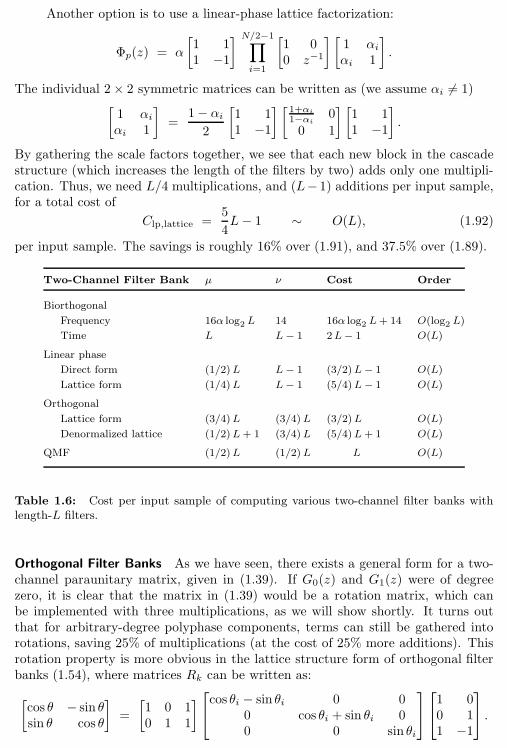
44 Chapter 1. Filter Banks: Building Blocks of Time-Frequency Expansions
Another option is to use a linear-phase lattice factorization:
Φp(z) = α
[1 11 −1
] N/2−1∏
i=1
[1 00 z−1
] [1 αiαi 1
].
The individual 2× 2 symmetric matrices can be written as (we assume αi 6= 1)[1 αiαi 1
]=
1− αi2
[1 11 −1
] [ 1+αi1−αi 0
0 1
] [1 11 −1
].
By gathering the scale factors together, we see that each new block in the cascadestructure (which increases the length of the filters by two) adds only one multipli-cation. Thus, we need L/4 multiplications, and (L− 1) additions per input sample,for a total cost of
Clp,lattice =5
4L− 1 ∼ O(L), (1.92)
per input sample. The savings is roughly 16% over (1.91), and 37.5% over (1.89).
Two-Channel Filter Bank µ ν Cost Order
Biorthogonal
Frequency 16α log2 L 14 16α log2 L+ 14 O(log2 L)
Time L L− 1 2L− 1 O(L)
Linear phase
Direct form (1/2)L L− 1 (3/2)L− 1 O(L)
Lattice form (1/4)L L− 1 (5/4)L− 1 O(L)
Orthogonal
Lattice form (3/4)L (3/4)L (3/2)L O(L)
Denormalized lattice (1/2)L+ 1 (3/4)L (5/4)L+ 1 O(L)
QMF (1/2)L (1/2)L L O(L)
Table 1.6: Cost per input sample of computing various two-channel filter banks withlength-L filters.
Orthogonal Filter Banks As we have seen, there exists a general form for a two-channel paraunitary matrix, given in (1.39). If G0(z) and G1(z) were of degreezero, it is clear that the matrix in (1.39) would be a rotation matrix, which canbe implemented with three multiplications, as we will show shortly. It turns outthat for arbitrary-degree polyphase components, terms can still be gathered intorotations, saving 25% of multiplications (at the cost of 25% more additions). Thisrotation property is more obvious in the lattice structure form of orthogonal filterbanks (1.54), where matrices Rk can be written as:
[cos θ − sin θsin θ cos θ
]=
[1 0 10 1 1
]cos θi − sin θi 0 0
0 cos θi + sin θi 00 0 sin θi
1 00 11 −1
.
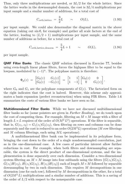
1.7. Computational Aspects 45
Thus, only three multiplications are needed, or 3L/2 for the whole lattice. Sincethe lattice works in the downsampled domain, the cost is 3L/4 multiplications perinput sample and a similar number of additions, for a total cost of
Corth,lattice =3
2L ∼ O(L), (1.93)
per input sample. We could also denormalize the diagonal matrix in the aboveequation (taking out sin θi for example) and gather all scale factors at the end ofthe lattice, leading to (L/2 + 1) multiplications per input sample, and the samenumber of additions as before, for a total cost of
Corth,lattice,denorm =5
4L+ 1 ∼ O(L), (1.94)
per input sample.
QMF Filter Banks The classic QMF solution discussed in Exercise ??, besidesusing even-length linear phase filters, forces the highpass filter to be equal to thelowpass, modulated by (−1)n. The polyphase matrix is therefore:
Φp(z) =
[G0(z) G1(z)G0(z) −G1(z)
]=
[1 11 −1
] [G0(z) 0
0 G1(z)
],
where G0 and G1 are the polyphase components of G(z). The factorized form onthe right indicates that the cost is halved. However, this scheme only approxi-mates a basis expansion (perfect reconstruction) when using FIR filters. Table 1.6summarizes the costs of various filter banks we have seen so far.
Multidimensional Filter Banks While we have not discussed multidimensionalfilter banks so far (some pointers are given in Further Reading), we do touch uponthe cost of computing them. For example, filtering an M ×M image with a filter oflength L×L requires of the order of O(M2 L2) operations. If the filter is separable,that is, G(z1, z2) = G1(z1)G2(z2), then filtering on rows and columns can be doneseparately and the cost is reduced to an orderO(2M2L) operations (M row filteringsand M column filterings, each using ML operations).
A multidimensional filter bank can be implemented in its polyphase form,bringing the cost down to the order of a single nondownsampled convolution, justas in the one-dimensional case. A few cases of particular interest allow furtherreductions in cost. For example, when both filters and downsampling are sepa-rable, the system is the direct product of one-dimensional systems, and the im-plementation is done separately over each dimension. Consider a two-dimensionalsystem filtering an M ×M image into four subbands using the filters G(z1)G(z2),G(z1)H(z2), H(z1)G(z2), H(z1)H(z2) each of lengthM×M followed by separabledownsampling by two in each dimension. This requires M decompositions in onedimension (one for each row), followed byM decompositions in the other, for a totalof O(2M2 L) multiplications and a similar number of additions. This is a saving ofthe order of L/2 with respect to the nonseparable case.
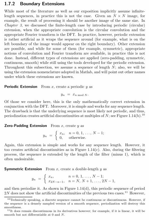
46 Chapter 1. Filter Banks: Building Blocks of Time-Frequency Expansions
1.7.2 Boundary Extensions
While most of the literature as well as our exposition implicitly assume infinite-length sequences, in practice this is not the case. Given an N × N image, forexample, the result of processing it should be another image of the same size. InChapter 3, we discussed the finite-length case by introducing periodic (circular)extension, when the appropriate convolution is the circular convolution and theappropriate Fourier transform is the DFT. In practice, however, periodic extensionis rather artificial as it wraps the sequence around (for example, what is on theleft boundary of the image would appear on the right boundary). Other extensionare possible, and while for some of them (for example, symmetric), appropriatenotions of convolution and Fourier transform are available, in practice this is notdone. Instead, different types of extensions are applied (zero-padding, symmetric,continuous, smooth) while still using the tools developed for the periodic extension.Throughout this subsection, we assume a sequence of length N ; also, we will beusing the extension nomenclature adopted in Matlab, and will point out other namesunder which these extensions are known.
Periodic Extension From x, create a periodic y as
yn = xn mod N .
Of those we consider here, this is the only mathematically correct extension inconjunction with the DFT. Moreover, it is simple and works for any sequence length.The drawback is that the underlying sequence is most likely not periodic, and thus,periodization creates artificial discontinuities at multiples ofN ; see Figure 1.14(b).10
Zero-Padding Extension From x, create y as
yn =
xn, n = 0, 1, . . . , N − 1;0, otherwise.
Again, this extension is simple and works for any sequence length. However, ittoo creates artificial discontinuities as in Figure 1.14(c). Also, during the filteringprocess, the sequence is extended by the length of the filter (minus 1), which isoften undesirable.
Symmetric Extension From x, create a double-length y as
yn =
xn, n = 0, 1, . . . , N − 1;x2N−n−1, n = N, N + 1, . . . , 2N − 1,
and then periodize it. As shown in Figure 1.14(d), this periodic sequence of period2N does not show the artificial discontinuities of the previous two cases.11 However,
10Technically speaking, a discrete sequence cannot be continuous or discontinuous. However, ifthe sequence is a densely sampled version of a smooth sequence, periodization will destroy thissmoothness.
11It does remain discontinuous in its derivatives however; for example, if it is linear, it will besmooth but not differentiable at 0 and N .
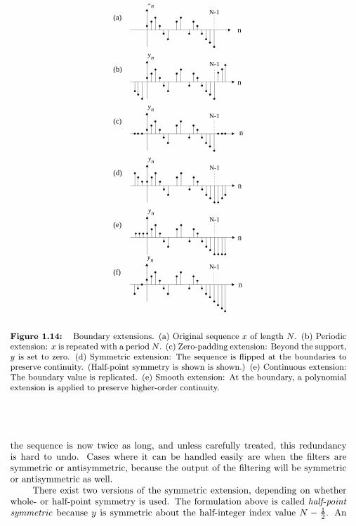
1.7. Computational Aspects 47
(a)
n
(b)
(c)
(d)
xnN-1
n
yn
n
yn
n
yn
n
yn
(f)
N-1
N-1
N-1
N-1
(e)
n
ynN-1
Figure 1.14: Boundary extensions. (a) Original sequence x of length N . (b) Periodicextension: x is repeated with a period N . (c) Zero-padding extension: Beyond the support,y is set to zero. (d) Symmetric extension: The sequence is flipped at the boundaries topreserve continuity. (Half-point symmetry is shown is shown.) (e) Continuous extension:The boundary value is replicated. (e) Smooth extension: At the boundary, a polynomialextension is applied to preserve higher-order continuity.
the sequence is now twice as long, and unless carefully treated, this redundancyis hard to undo. Cases where it can be handled easily are when the filters aresymmetric or antisymmetric, because the output of the filtering will be symmetricor antisymmetric as well.
There exist two versions of the symmetric extension, depending on whetherwhole- or half-point symmetry is used. The formulation above is called half-pointsymmetric because y is symmetric about the half-integer index value N − 1
2 . An
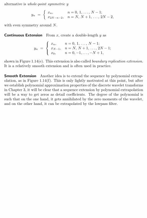
48 Chapter 1. Filter Banks: Building Blocks of Time-Frequency Expansions
alternative is whole-point symmetric y
yn =
xn, n = 0, 1, . . . , N − 1;x2N−n−2, n = N, N + 1, . . . , 2N − 2,
with even symmetry around N .
Continuous Extension From x, create a double-length y as
yn =
xn, n = 0, 1, . . . , N − 1;xN−1, n = N, N + 1, . . . , 2N − 1;x0, n = 0,−1, . . . ,−N + 1,
shown in Figure 1.14(e). This extension is also called boundary replication extension.It is a relatively smooth extension and is often used in practice.
Smooth Extension Another idea is to extend the sequence by polynomial extrap-olation, as in Figure 1.14(f). This is only lightly motivated at this point, but afterwe establish polynomial approximation properties of the discrete wavelet transformsin Chapter 3, it will be clear that a sequence extension by polynomial extrapolationwill be a way to get zeros as detail coefficients. The degree of the polynomial issuch that on the one hand, it gets annihilated by the zero moments of the wavelet,and on the other hand, it can be extrapolated by the lowpass filter.
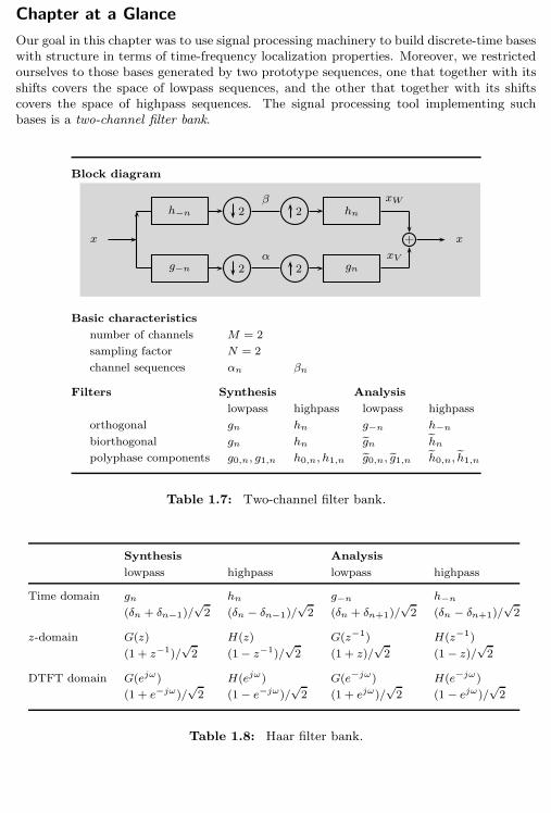
Chapter at a Glance 49
Chapter at a Glance
Our goal in this chapter was to use signal processing machinery to build discrete-time baseswith structure in terms of time-frequency localization properties. Moreover, we restrictedourselves to those bases generated by two prototype sequences, one that together with itsshifts covers the space of lowpass sequences, and the other that together with its shiftscovers the space of highpass sequences. The signal processing tool implementing suchbases is a two-channel filter bank.
Block diagram
x
h−n 2β
2 hn
g−n 2α
2 gn
xW
xV
+ x
Basic characteristics
number of channels M = 2
sampling factor N = 2
channel sequences αn βn
Filters Synthesis Analysis
lowpass highpass lowpass highpass
orthogonal gn hn g−n h−nbiorthogonal gn hn gn hn
polyphase components g0,n, g1,n h0,n, h1,n g0,n, g1,n h0,n, h1,n
Table 1.7: Two-channel filter bank.
Synthesis Analysis
lowpass highpass lowpass highpass
Time domain gn hn g−n h−n(δn + δn−1)/
√2 (δn − δn−1)/
√2 (δn + δn+1)/
√2 (δn − δn+1)/
√2
z-domain G(z) H(z) G(z−1) H(z−1)
(1 + z−1)/√2 (1− z−1)/
√2 (1 + z)/
√2 (1 − z)/
√2
DTFT domain G(ejω) H(ejω) G(e−jω) H(e−jω)
(1 + e−jω)/√2 (1− e−jω)/
√2 (1 + ejω)/
√2 (1 − ejω)/
√2
Table 1.8: Haar filter bank.
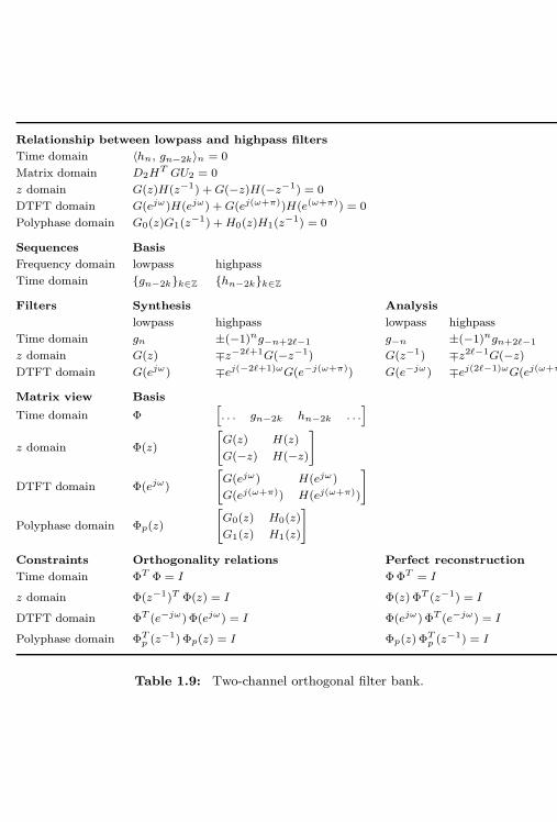
50 Chapter 1. Filter Banks: Building Blocks of Time-Frequency Expansions
Relationship between lowpass and highpass filters
Time domain 〈hn, gn−2k〉n = 0
Matrix domain D2HT GU2 = 0
z domain G(z)H(z−1) +G(−z)H(−z−1) = 0
DTFT domain G(ejω)H(ejω) +G(ej(ω+π))H(e(ω+π)) = 0
Polyphase domain G0(z)G1(z−1) +H0(z)H1(z
−1) = 0
Sequences Basis
Frequency domain lowpass highpass
Time domain gn−2kk∈Z hn−2kk∈Z
Filters Synthesis Analysis
lowpass highpass lowpass highpass
Time domain gn ±(−1)ng−n+2ℓ−1 g−n ±(−1)ngn+2ℓ−1
z domain G(z) ∓z−2ℓ+1G(−z−1) G(z−1) ∓z2ℓ−1G(−z)DTFT domain G(ejω) ∓ej(−2ℓ+1)ωG(e−j(ω+π)) G(e−jω) ∓ej(2ℓ−1)ωG(ej(ω+π))
Matrix view Basis
Time domain Φ[. . . gn−2k hn−2k . . .
]
z domain Φ(z)
[G(z) H(z)
G(−z) H(−z)
]
DTFT domain Φ(ejω)
[G(ejω) H(ejω)
G(ej(ω+π)) H(ej(ω+π))
]
Polyphase domain Φp(z)
[G0(z) H0(z)
G1(z) H1(z)
]
Constraints Orthogonality relations Perfect reconstruction
Time domain ΦT Φ = I ΦΦT = I
z domain Φ(z−1)T Φ(z) = I Φ(z) ΦT (z−1) = I
DTFT domain ΦT (e−jω)Φ(ejω) = I Φ(ejω)ΦT (e−jω) = I
Polyphase domain ΦTp (z−1) Φp(z) = I Φp(z) Φ
Tp (z
−1) = I
Table 1.9: Two-channel orthogonal filter bank.
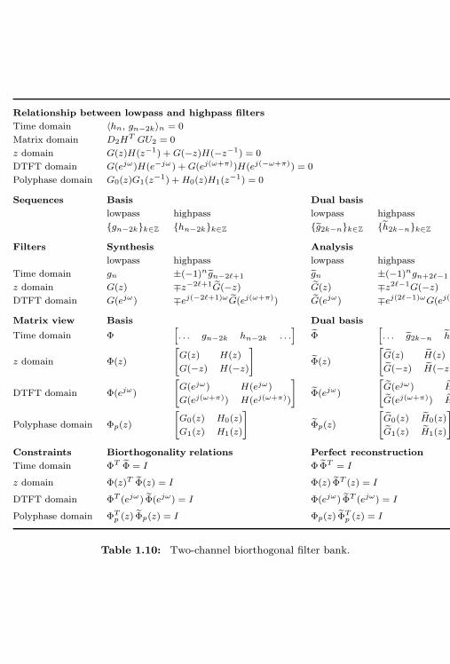
Chapter at a Glance 51
Relationship between lowpass and highpass filters
Time domain 〈hn, gn−2k〉n = 0
Matrix domain D2HT GU2 = 0
z domain G(z)H(z−1) +G(−z)H(−z−1) = 0
DTFT domain G(ejω)H(e−jω) +G(ej(ω+π))H(ej(−ω+π)) = 0
Polyphase domain G0(z)G1(z−1) +H0(z)H1(z
−1) = 0
Sequences Basis Dual basis
lowpass highpass lowpass highpass
gn−2kk∈Z hn−2kk∈Z g2k−nk∈Z h2k−nk∈Z
Filters Synthesis Analysis
lowpass highpass lowpass highpass
Time domain gn ±(−1)n gn−2ℓ+1 gn ±(−1)ngn+2ℓ−1
z domain G(z) ∓z−2ℓ+1G(−z) G(z) ∓z2ℓ−1G(−z)DTFT domain G(ejω) ∓ej(−2ℓ+1)ωG(ej(ω+π)) G(ejω) ∓ej(2ℓ−1)ωG(ej(ω+π))
Matrix view Basis Dual basis
Time domain Φ[. . . gn−2k hn−2k . . .
]Φ
[. . . g2k−n h2k−n . . .
]
z domain Φ(z)
[G(z) H(z)
G(−z) H(−z)
]Φ(z)
[G(z) H(z)
G(−z) H(−z)
]
DTFT domain Φ(ejω)
[G(ejω) H(ejω)
G(ej(ω+π)) H(ej(ω+π))
]Φ(ejω)
[G(ejω) H(ejω)
G(ej(ω+π)) H(ej(ω+π))
]
Polyphase domain Φp(z)
[G0(z) H0(z)
G1(z) H1(z)
]Φp(z)
[G0(z) H0(z)
G1(z) H1(z)
]
Constraints Biorthogonality relations Perfect reconstruction
Time domain ΦT Φ = I ΦΦT = I
z domain Φ(z)T Φ(z) = I Φ(z) ΦT (z) = I
DTFT domain ΦT (ejω) Φ(ejω) = I Φ(ejω) ΦT (ejω) = I
Polyphase domain ΦTp (z) Φp(z) = I Φp(z) ΦTp (z) = I
Table 1.10: Two-channel biorthogonal filter bank.
52 Chapter 1. Filter Banks: Building Blocks of Time-Frequency Expansions
Historical Remarks
Filter banks have been popular in signal processing since the
1970s when the question of critically-sampled filter banks, those
with the number of channel samples per unit of time conserved,
arose in the context of subband coding of speech. In that method,
a speech sequence is split into downsampled frequency bands, al-
lowing for more powerful compression. However, downsampling
can create a perceptually disturbing effect known as aliasing, prompting Esteban and Ga-
land [38] in 1977 to propose a simple and elegant quadrature mirror filters (QMF) aliasing-
removal technique. As QMF solution does not allow for perfect reconstruction, a flurry of
work followed to solve the problem. Mintzer [64] as well Smith and Barnwell [83] proposed
an orthogonal solution independently in the mid 1980s. Vaidyanathan [96] established
a connection to lossless systems, unveiling the factorization and design of paraunitary
matrices [100]. For wavelet purposes, Daubechies then designed filters with a maximum
number of zeros at z = −1 [29], a solution that goes back to Herrmann’s design of maxi-
mally flat FIR filters [47]. The equivalent IIR filter design problem leads to Butterworth
filters, as derived by Herley and Vetterli [45]. Vetterli solved the biorthogonal filter bank
problem [103, 104], while Cohen, Daubechies and Feauveau [23] as well as Vetterli and
Herley [105] tackled those with maximum number of zeros at z = −1. The polyphase
framework was used by many authors working on filter banks, but really goes back to ear-
lier work on transmultiplexers by Bellanger and Daguet [7]. The realization that perfect
reconstruction subband coding can be used for perfect transmultiplexing appears in [104].
The idea of multichannel structures that can be inverted perfectly, including with quanti-
zation, goes back to ladder structures in filter design and implementation, in the works of
Bruckens and van den Enden, Marshall, Shah and Kalker [14,62,79]. Sweldens generalized
this idea under the name of lifting [90], deriving a number of new schemes based on this
concept, including filter banks with nonlinear operators and nonuniform sampling.
Further Reading
Books and Textbooks A few standard textbooks on filter banks exist, written byVaidyanathan [98], Vetterli and Kovacevic [106], Strang and Nguyen [87], among others.
N -Channel Filter Banks One of the important and immediate generalizations of two-channel filter banks is when we allow the number of channels to be N . Numerous op-tions are available, from directly designing N-channel filter banks, studied in detail byVaidyanathan [96,97], through those built by cascading filter banks with different numberof branches, leading to almost arbitrary frequency divisions. The analysis methods fol-low closely those of the two-channel filter banks, albeit with more freedom; for example,orthogonality and linear phase are much easier to achieve at the same time. We discussN-channel filter banks in detail in Chapter 2, with special emphasis on local Fourier bases.
Multidimensional Filter Banks The first difference we encounter when dealing withmultidimensional filter banks is that of sampling. Regular sampling with a given densitycan be accomplished using any number of sampling lattices, each having any number ofassociated sampling matrices. These have been described in detail by Dubois in [35], and
Further Reading 53
have been used by Viscito and Allebach [109], Karlsson and Vetterli [50], Kovacevic andVetterli [55], Do and Vetterli [33], among others, to design multidimensional filter banks.Apart from the freedom coming with different sampling schemes, the associated filters cannow be truly multidimensional, allowing for a much larger space of solutions.
IIR Filter Banks While IIR filters should be of importance because of their good fre-quency selectivity and computational efficiency, they have not been used extensively astheir implementation in a filter-bank framework comes at a cost: one side of the filter bankis necessarily anticausal. They have found some use in image processing as the finite lengthof the input allows for storing the state in the middle of the filter bank and synthesizingfrom that stored state. Coverage of IIR filter banks can be found in [45,70,82].
Oversampled Filter Banks Yet another generalization occurs when we allow for re-dundancy, leading to overcomplete filter banks implementing frame expansions, coveredin Chapter 4. These filter banks are becoming popular in applications due to inherentfreedom in design.
Complex-Coefficient Filter Banks This entire chapter dealt exclusively with real-coefficient filter banks, due to their prevalence in practice. Complex-coefficient filter banksexist, from the very early QMFs [66] to more recent ones, mostly in the form of complexexponential-modulated local Fourier bases, discussed in Section 2.3, as well as the redun-dant ones, such as Gabor frames [10–12,26,39], discussed in Chapter 4.
QMF Filter Banks QMF filter banks showed the true potential of filter banks, as it wasclear that one could have nonideal filters and still split and reconstruct the input spectrum.The excitement was further spurred by the famous linear-phase designs by Johnston [49]in 1980. Exercise ?? discusses derivation of these filters and their properties.
Time-Varying Filter Banks and Boundary Filters The periodic shift variance of filterbanks can be exploited to change a filter bank essentially every period. This was done foryears in audio coding through the so-called MDCT filter banks, discussed in Section 2.4.1.Herley and Vetterli proposed a more formal approach in [46], by designing different filtersto be used at the boundary of a finite-length input, or a filter-bank change.
Transmultiplexing The dual scheme to a filter bank is known as a transmultiplexer,where two sequences are synthesized into a combined sequence from which the two partscan be extracted perfectly. An orthogonal decomposition with many channels leads to or-thogonal frequency-division multiplexing (OFDM), the basis for many modulation schemesused in communications, such as 802.11. The analysis of transmultiplexers uses similartools as for filter banks [104], covered in Solved Exercise ?? for the orthogonal case, andin Exercise ?? for the biorthogonal case. Exercise ?? considers frequency-division multi-plexing with Haar filters.
Filter Banks with Stochastic Inputs Among the wealth of filter banks available, itis often necessary to determine which one is the most suitable for a given application.A number of measures have been proposed, for example, quantifying shift variance ofsubband energies for deterministic inputs. Similarly, in [1,2], the author proposes, amongothers, a counterpart measure based on the cyclostationarity of subband powers. We donot dwell on these here, rather we leave the discussion for Chapter 7. Akkarakaran and
54 Chapter 1. Filter Banks: Building Blocks of Time-Frequency Expansions
Vaidyanathan in [4] discuss bifrequency and bispectrum maps (deterministic and stochastictime-varying autocorrelations) in filter banks and answer many relevant questions; somesimilar issues are tackled by Therrien in [91]. In [99], Vaidyanathan and Akkarakarangive a review of optimal filter banks based on input statistics. In particular, principal-component filter banks offer optimal solutions to various problems, some of these discussedin [93] and [94,95].
Chapter 2
Local Fourier Bases on
Sequences
Contents
2.1 Introduction 56
2.2 N-Channel Filter Banks 59
2.3 Complex Exponential-Modulated Local FourierBases 66
2.4 Cosine-Modulated Local Fourier Bases 75
2.5 Computational Aspects 85
Chapter at a Glance 87
Historical Remarks 88
Further Reading 90
Think of a piece of music: notes appear at different instants of time, and thenfade away. These are short-time frequency events the human ear identifies easily,but are a challenge for a computer to understand. These notes are well identifiedfrequencies, but they are short lived. Thus, we would like to have access to alocal Fourier transform, that is, a time-frequency analysis tool that understands thespectrum locally in time. While such a transform is known under many names, suchas windowed Fourier transform, Gabor transform and short-time Fourier transform,we will use local Fourier transform exclusively throughout the manuscript. Thelocal energy distribution over frequency, which can be obtained by squaring themagnitude of the local Fourier coefficients, is called the spectrogram, and is widelyused in speech processing and time-series analysis.
Our purpose in this chapter is to explore what is possible in terms of obtainingsuch a local version of the Fourier transform of a sequence. While, unfortunately, wewill see that, apart from short ones, there exist no good longer local Fourier bases,there exist good local Fourier frames, the topic we explore in Chapter 4. Moreover,there exist good local cosine bases, where the complex-exponential modulation isreplaced by cosine modulation. These constructions will all be implemented usinggeneral, N -channel filter banks, the first generalization of the basic two-channelfilter bank block we just saw in the last chapter.
55
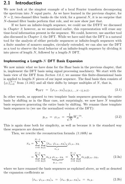
56 Chapter 2. Local Fourier Bases on Sequences
2.1 Introduction
We now look at the simplest example of a local Fourier transform decomposingthe spectrum into N equal parts. As we have learned in the previous chapter, forN = 2, two-channel filter banks do the trick; for a general N , it is no surprise thatN -channel filter banks perform that role, and we now show just that.
If we have an infinite-length sequence, we could use the DTFT we discussedin Chapter 3; however, as we mentioned earlier, this representation will erase anytime-local information present in the sequence. We could, however, use another toolalso discussed in Chapter 3, the DFT. While we have said that the DFT is a naturaltool for the analysis of either periodic sequences or infinite-length sequences witha finite number of nonzero samples, circularly extended, we can also use the DFTas a tool to observe the local behavior of an infinite-length sequence by dividing itinto pieces of length N , followed by a length-N DFT.
Implementing a Length-N DFT Basis Expansion
We now mimic what we have done for the Haar basis in the previous chapter, thatis, implement the DFT basis using signal processing machinery. We start with thebasis view of the DFT from Section 3.6.1; we assume this finite-dimensional basisis applied to length-N pieces of our input sequence. The final basis then consists ofϕiN−1
i=0 from (3.162) and all their shifts by integer multiples of N , that is,
ΦDFT = ϕi,n−Nki∈0,1,...,N−1,k∈Z. (2.1)
In other words, as opposed to two template basis sequences generating the entirebasis by shifting as in the Haar case, not surprisingly, we now have N templatebasis sequences generating the entire basis by shifting. We rename those templatebasis sequences to (we use the normalized version of the DFT):
gi,n = ϕi,n =1√NW−inN
. (2.2)
This is again done both for simplicity, as well as because it is the standard waythese sequences are denoted.
Then, we rewrite the reconstruction formula (3.160b) as
xn =
N−1∑
i=0
∑
k∈Z
〈xn, ϕi,n−Nk〉n︸ ︷︷ ︸αi,k
ϕi,n−Nk
=
N−1∑
i=0
∑
k∈Z
αi,k ϕi,n−Nk︸ ︷︷ ︸gi,n−Nk
=
N−1∑
i=0
∑
k∈Z
αi,kgi,n−Nk, (2.3a)
where we have renamed the basis sequences as explained above, as well as denotedthe expansion coefficients as
〈xn, ϕi,n−Nk〉n = 〈xn, gi,n−Nk〉n = αi,k. (2.3b)
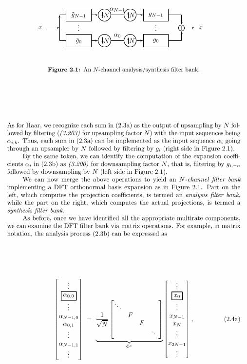
2.1. Introduction 57
x
gN−1 NαN−1
N gN−1
g0 Nα0
N g0
...... + x
Figure 2.1: An N-channel analysis/synthesis filter bank.
As for Haar, we recognize each sum in (2.3a) as the output of upsampling by N fol-lowed by filtering ((3.203) for upsampling factor N) with the input sequences beingαi,k. Thus, each sum in (2.3a) can be implemented as the input sequence αi goingthrough an upsampler by N followed by filtering by gi (right side in Figure 2.1).
By the same token, we can identify the computation of the expansion coeffi-cients αi in (2.3b) as (3.200) for downsampling factor N , that is, filtering by gi,−nfollowed by downsampling by N (left side in Figure 2.1).
We can now merge the above operations to yield an N -channel filter bankimplementing a DFT orthonormal basis expansion as in Figure 2.1. Part on theleft, which computes the projection coefficients, is termed an analysis filter bank,while the part on the right, which computes the actual projections, is termed asynthesis filter bank.
As before, once we have identified all the appropriate multirate components,we can examine the DFT filter bank via matrix operations. For example, in matrixnotation, the analysis process (2.3b) can be expressed as
...α0,0
...αN−1,0
α0,1
...αN−1,1
...
=1√N
. . .
FF
. . .
︸ ︷︷ ︸Φ∗
...x0...
xN−1
xN...
x2N−1
...
, (2.4a)
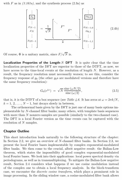
58 Chapter 2. Local Fourier Bases on Sequences
with F as in (3.161a), and the synthesis process (2.3a) as
...x0...
xN−1
xN...
x2N−1
...
=1√N
. . .
F ∗
F ∗
. . .
︸ ︷︷ ︸Φ
...α0,0
...αN−1,0
α0,1
...αN−1,1
...
. (2.4b)
Of course, Φ is a unitary matrix, since F/√N is.
Localization Properties of the Length-N DFT It is quite clear that the timelocalization properties of the DFT are superior to those of the DTFT, as now, wehave access to the time-local events at the resolution of length N . However, as aresult, the frequency resolution must necessarily worsen; to see this, consider thefrequency response of g0 (the other gks are modulated versions and therefore havethe same frequency resolution):
G0(ejω) =
√N
sinc (ωN/2)
sinc (ω/2), (2.5)
that is, it is the DTFT of a box sequence (see Table 4.6. It has zeros at ω = 2πk/N ,k = 1, 2, . . . , N − 1, but decays slowly in between.
The orthonormal basis given by the DFT is just one of many basis options im-plementable by N -channel filter banks; many others, with template basis sequenceswith more than N nonzero samples are possible (similarly to the two-channel case).The DFT is a local Fourier version as the time events can be captured with theresolution of N samples.
Chapter Outline
This short introduction leads naturally to the following structure of the chapter:In Section 2.2, we give an overview of N -channel filter banks. In Section 2.3, wepresent the local Fourier bases implementable by complex exponential-modulatedfilter banks. We then come to the crucial, albeit negative result: the Balian-Lowtheorem, which states the impossibility of good complex exponential-modulatedlocal Fourier bases. We look into their applications: local power spectral density viaperiodograms, as well as in transmultiplexing. To mitigate the Balian-Low negativeresult, Section 2.4 considers what happens if we use cosine modulation insteadof the complex one to obtain a local frequency analysis. In the block-transformcase, we encounter the discrete cosine transform, which plays a prominent role inimage processing. In the sliding window case, a cosine-modulated filter bank allows

2.2. N -Channel Filter Banks 59
the best of both worlds, namely an orthonormal basis with good time-frequencylocalization. We also discuss variations on this construction as well as an applicationto audio compression.
Notation used in this chapter: Unlike in the previous chapter, in this one, complex-coefficient filter banks are the norm. Thus, Hermitian transposition is used often,with the caveat that only coefficients should be conjugated and not z. We will pointthese out throughout the chapter.
2.2 N-Channel Filter Banks
We could imagine achieving our goal of splicing the spectrum into N pieces manyways; we have just seen one, achievable by using the DFT, a representation withreasonable time but poor frequency localization. Another option is using an idealNth band filter and its shifts (we have seen it in Table 3.5 and Table 4.6, as well as(3.108) with ω0 = 2π/N , but repeat it here for completeness):
g0,n =1√N
sinc(πn/N)DTFT←→ G0(e
jω) =
√N, |ω| ≤ π/N ;0, otherwise,
(2.6)
which clearly has perfect frequency localization but poor time localization as itsimpulse response is a discrete sinc sequence. We have discussed this trade-off alreadyin Chapter 7, and depict it in Figure 2.2.
The question now is whether there exist constructions in between these twoextreme cases? Specifically, are there basis sequences with better frequency local-ization than the block transform, but with impulse responses that decay faster thanthe sinc impulse response (for example, a finite impulse response)?
To explore this issue, we introduce generalN -channel filter banks. These are asshown in Figure 2.1, where the input is analyzed by N filters gi, i = 0, 1, . . . , N−1,and downsampled by N . The synthesis is done by upsampling by N , followed byinterpolation with gi, i = 0, 1, . . . , N − 1.
The analysis of N -channel filter banks can be done in complete analogy to thetwo-channel case, by using the relevant equations for sampling rate changes by N .We now state these without proofs, and illustrate them on a particular case of a3-channel filter bank, especially in polyphase domain.
2.2.1 Orthogonal N-Channel Filter Banks
As for two-channel filter banks, N -channel orthogonal filter banks are of particularinterest; the DFT is one example. We now briefly follow the path from the previouschapter and put in one place the relations governing such filter banks. The biorthog-onal ones follow similarly, and we just touch upon them during the discussion ofthe polyphase view.
Orthogonality of a Single Filter Since we started with an orthonormal basis, theset gi,n−Nkk∈Z,i∈0,1,...,N−1 is an orthonormal set. We have seen in Section 3.7.4
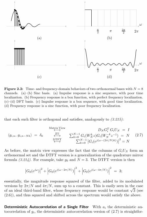
60 Chapter 2. Local Fourier Bases on Sequences
π
2 π 3π2 2π
ω
(a) (b)
π
2 π 3π2 2π
ω
(c) (d)
Figure 2.2: Time- and frequency-domain behaviors of two orthonormal bases with N = 8channels. (a)–(b) Sinc basis. (a) Impulse response is a sinc sequence, with poor timelocalization. (b) Frequency response is a box function, with perfect frequency localization.(c)–(d) DFT basis. (c) Impulse response is a box sequence, with good time localization.(d) Frequency response is a sinc function, with poor frequency localization.
that each such filter is orthogonal and satisfies, analogously to (3.215):
〈gi,n, gi,n−Nk〉 = δk
MatrixView←→ DNGT
iGiUN = I
ZT←→ ∑N−1k=0 Gi(W
k
Nz)Gi(W
−kNz−1) = N
DTFT←→ ∑N−1k=0
∣∣Gi(ej(ω−(2π/N)k))∣∣2 = N
(2.7)
As before, the matrix view expresses the fact that the columns of GiUN form anorthonormal set and the DTFT version is a generalization of the quadrature mirrorformula (3.214). For example, take g0 and N = 3. The DTFT version is then
∣∣G0(ejω)∣∣2 +
∣∣∣G0(ej(ω−2π/N))
∣∣∣2
+∣∣∣G0(e
j(ω−4π/N))∣∣∣2
= 3;
essentially, the magnitude response squared of the filter, added to its modulatedversions by 2π/N and 4π/N , sum up to a constant. This is easily seen in the caseof an ideal third-band filter, whose frequency response would be constant
√3 (see
(2.6)), and thus squared and shifted across the spectrum would satisfy the above.
Deterministic Autocorrelation of a Single Filter With ai the deterministic au-tocorrelation of gi, the deterministic autocorrelation version of (2.7) is straightfor-
2.2. N -Channel Filter Banks 61
ward:
〈gi,n, gi,n−Nk〉 = ai,Nk = δk
MatrixView←→ DNAiUN = IZT←→
∑N−1k=0 Ai(W
k
Nz) = N
DTFT←→ ∑N−1k=0 Ai(e
j(ω−(2π/N)k)) = N(2.8)
Orthogonal Projection Property a Single Channel Analogously to two channels,a single channel with orthogonal filters projects onto a coarse subspace V0 or detailsubspaces Wi, i = 1, 2, . . . , N − 1, depending on the frequency properties of thefilter. Each of the orthogonal projection operators is given as
PV0 = G0UN DNGT
0 ,
PWi= GiUN DNG
T
i, i = 1, 2, . . . , N − 1,
with the range
V0 = span(g0,n−Nkk∈Z),
Wi = span(gi,n−Nkk∈Z), i = 1, 2, . . . , N − 1.
Orthogonality of Filters As in the previous chapter, once the orthonormality ofeach single channel is established, what is left is the orthogonality of the channelsamong themselves. Again, all the expressions are analogous to the two-channel case;we state them here without proof. We assume below that i 6= j.
〈gi,n, gj,n−Nk〉 = 0
MatrixView←→ DNGT
jGiUN = 0
ZT←→ ∑N−1k=0 Gi(W
k
Nz)Gj(W
−kNz−1) = 0
DTFT←→ ∑N−1k=0 Gi(e
j(ω−(2π/N)k))Gj(e−j(ω+(2π/N)k)) = 0
(2.9)
Deterministic Crosscorrelation of Filters Calling ci,j the deterministic crosscor-relation of gi and gj:
〈gi,n, gj,n−Nk〉 = ci,j,Nk = 0
MatrixView←→ DNCi,jUN = 0ZT←→ ∑
N−1k=0 Ci,j(W
k
Nz) = 0
DTFT←→ ∑N−1k=0 Ci,j(e
j(ω−(2π/N)k)) = 0(2.10)
2.2.2 Polyphase View of N-Channel Filter Banks
To cover the polyphase view for general N , we cover it through an example withN = 3, and then briefly summarize the discussion for a general N .

62 Chapter 2. Local Fourier Bases on Sequences
Example 2.1 (Orthogonal 3-channel filter banks) For two-channel fil-ter banks, a polyphase decomposition is achieved by simply splitting both se-quences and filters into their even- and odd-indexed subsequences; for 3-channelfilter banks, we split sequences and filters into subsequences modulo 3. Whilewe have seen the expression for a polyphase representation of a sequence andfilters for a general N in (3.227), we write them out for N = 3 to develop someintuition, starting with the input sequence x:
x0,n = x3nZT←→ X0(z) =
∑
n∈Z
x3n z−n,
x1,n = x3n+1ZT←→ X1(z) =
∑
n∈Z
x3n+1 z−n,
x2,n = x3n+2ZT←→ X2(z) =
∑
n∈Z
x3n+2 z−n,
X(z) = X0(z3) + z−1X1(z
3) + z−2X2(z3).
In the above, x0 is the subsequence of x at multiples of 3 downsampled by 3, andsimilarly for x1 and x2:
x0 =[. . . x−3 x0 x3 x6 . . .
]T,
x1 =[. . . x−2 x1 x4 x7 . . .
]T,
x2 =[. . . x−1 x2 x5 x8 . . .
]T.
This is illustrated in Figure 2.3(a): to get x0 we simply keep every third samplefrom x; to get x1, we shift x by one to the left (advance by one represented byz) and then keep every third sample; finally, to get x2, we shift x by two tothe left and then keep every third sample. To get the original sequence back,we upsample each subsequence by 3, shift appropriately to the right (delaysrepresented by z−1 and z−2), and sum up.
Using (3.227), we define the polyphase decomposition of the synthesis fil-ters:
gi,0,n = gi,3nZT←→ Gi,0(z) =
∑
n∈Z
gi,3n z−n, (2.11a)
gi,1,n = gi,3n+1ZT←→ Gi,1(z) =
∑
n∈Z
gi,3n+1 z−n, (2.11b)
gi,2,n = gi,3n+2ZT←→ Gi,2(z) =
∑
n∈Z
gi,3n+2 z−n, (2.11c)
Gi(z) = Gi,0(z3) + z−1Gi,1(z
3) + z−2Gi,2(z3),
where the first subscript denotes the filter, the second the polyphase component,and the last, the discrete time index. In the above, we split each synthesis filter
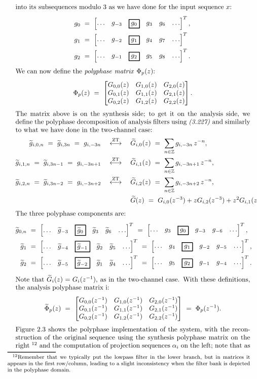
2.2. N -Channel Filter Banks 63
into its subsequences modulo 3 as we have done for the input sequence x:
g0 =[. . . g−3 g0 g3 g6 . . .
]T
,
g1 =[. . . g−2 g1 g4 g7 . . .
]T
g2 =[. . . g−1 g2 g5 g8 . . .
]T
.
We can now define the polyphase matrix Φp(z):
Φp(z) =
G0,0(z) G1,0(z) G2,0(z)G0,1(z) G1,1(z) G2,1(z)G0,2(z) G1,2(z) G2,2(z)
.
The matrix above is on the synthesis side; to get it on the analysis side, wedefine the polyphase decomposition of analysis filters using (3.227) and similarlyto what we have done in the two-channel case:
gi,0,n = gi,3n = gi,−3nZT←→ Gi,0(z) =
∑
n∈Z
gi,−3n z−n,
gi,1,n = gi,3n−1 = gi,−3n+1ZT←→ Gi,1(z) =
∑
n∈Z
gi,−3n+1 z−n,
gi,2,n = gi,3n−2 = gi,−3n+2ZT←→ Gi,2(z) =
∑
n∈Z
gi,−3n+2 z−n,
G(z) = Gi,0(z−3) + zGi,2(z
−3) + z2Gi,1(z−3).
The three polyphase components are:
g0,n =[. . . g−3 g0 g3 g6 . . .
]T
=[. . . g3 g0 g−3 g−6 . . .
]T
,
g1 =[. . . g−4 g−1 g2 g5 . . .
]T
=[. . . g4 g1 g−2 g−5 . . .
]T
,
g2 =[. . . g−5 g−2 g1 g4 . . .
]T
=[. . . g5 g2 g−1 g−4 . . .
]T
.
Note that Gi(z) = Gi(z−1), as in the two-channel case. With these definitions,
the analysis polyphase matrix i:
Φp(z) =
G0,0(z
−1) G1,0(z−1) G2,0(z
−1)G0,1(z
−1) G1,1(z−1) G2,1(z
−1)G0,2(z
−1) G1,2(z−1) G2,2(z
−1)
= Φp(z
−1).
Figure 2.3 shows the polyphase implementation of the system, with the recon-struction of the original sequence using the synthesis polyphase matrix on theright 12 and the computation of projection sequences αi on the left; note that as
12Remember that we typically put the lowpass filter in the lower branch, but in matrices itappears in the first row/column, leading to a slight inconsistency when the filter bank is depictedin the polyphase domain.
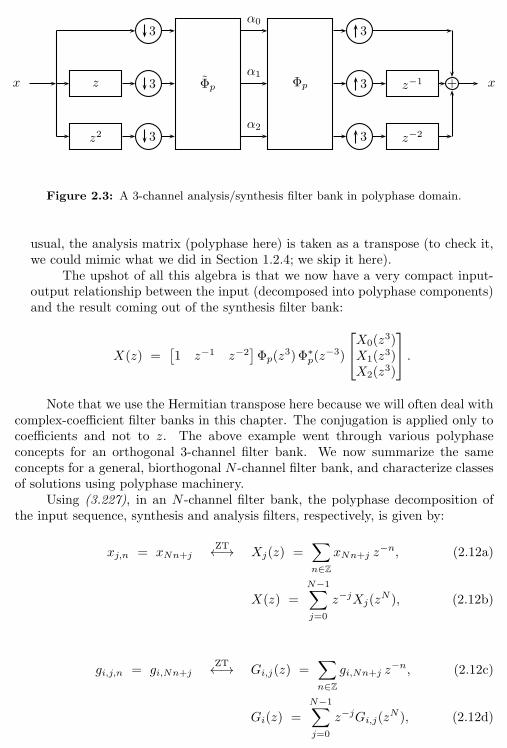
64 Chapter 2. Local Fourier Bases on Sequences
x
3α0
3
z 3 Φpα1
Φp 3 z−1 +
z2 3α2
3 z−2
x
Figure 2.3: A 3-channel analysis/synthesis filter bank in polyphase domain.
usual, the analysis matrix (polyphase here) is taken as a transpose (to check it,we could mimic what we did in Section 1.2.4; we skip it here).
The upshot of all this algebra is that we now have a very compact input-output relationship between the input (decomposed into polyphase components)and the result coming out of the synthesis filter bank:
X(z) =[1 z−1 z−2
]Φp(z
3)Φ∗p(z−3)
X0(z
3)X1(z
3)X2(z
3)
.
Note that we use the Hermitian transpose here because we will often deal withcomplex-coefficient filter banks in this chapter. The conjugation is applied only tocoefficients and not to z. The above example went through various polyphaseconcepts for an orthogonal 3-channel filter bank. We now summarize the sameconcepts for a general, biorthogonal N -channel filter bank, and characterize classesof solutions using polyphase machinery.
Using (3.227), in an N -channel filter bank, the polyphase decomposition ofthe input sequence, synthesis and analysis filters, respectively, is given by:
xj,n = xNn+jZT←→ Xj(z) =
∑
n∈Z
xNn+j z−n, (2.12a)
X(z) =N−1∑
j=0
z−jXj(zN ), (2.12b)
gi,j,n = gi,Nn+jZT←→ Gi,j(z) =
∑
n∈Z
gi,Nn+j z−n, (2.12c)
Gi(z) =
N−1∑
j=0
z−jGi,j(zN ), (2.12d)
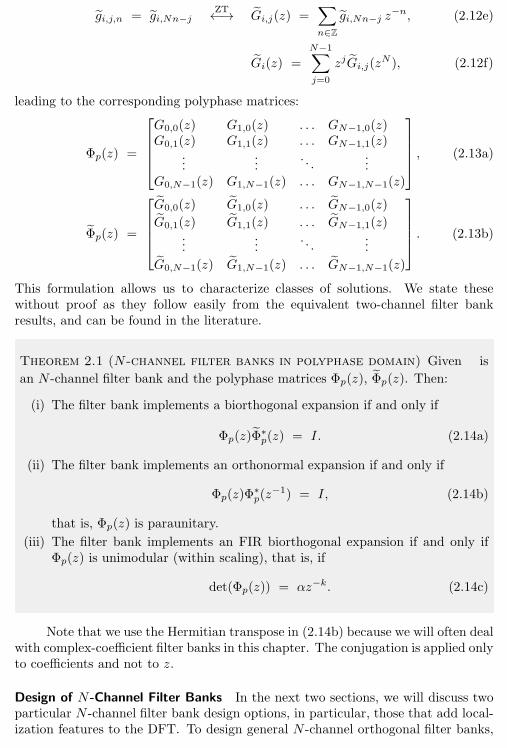
2.2. N -Channel Filter Banks 65
gi,j,n = gi,Nn−jZT←→ Gi,j(z) =
∑
n∈Z
gi,Nn−j z−n, (2.12e)
Gi(z) =
N−1∑
j=0
zjGi,j(zN ), (2.12f)
leading to the corresponding polyphase matrices:
Φp(z) =
G0,0(z) G1,0(z) . . . GN−1,0(z)G0,1(z) G1,1(z) . . . GN−1,1(z)
......
. . ....
G0,N−1(z) G1,N−1(z) . . . GN−1,N−1(z)
, (2.13a)
Φp(z) =
G0,0(z) G1,0(z) . . . GN−1,0(z)
G0,1(z) G1,1(z) . . . GN−1,1(z)...
.... . .
...
G0,N−1(z) G1,N−1(z) . . . GN−1,N−1(z)
. (2.13b)
This formulation allows us to characterize classes of solutions. We state thesewithout proof as they follow easily from the equivalent two-channel filter bankresults, and can be found in the literature.
Theorem 2.1 (N-channel filter banks in polyphase domain) Given is
an N -channel filter bank and the polyphase matrices Φp(z), Φp(z). Then:
(i) The filter bank implements a biorthogonal expansion if and only if
Φp(z)Φ∗p(z) = I. (2.14a)
(ii) The filter bank implements an orthonormal expansion if and only if
Φp(z)Φ∗p(z−1) = I, (2.14b)
that is, Φp(z) is paraunitary.
(iii) The filter bank implements an FIR biorthogonal expansion if and only ifΦp(z) is unimodular (within scaling), that is, if
det(Φp(z)) = αz−k. (2.14c)
Note that we use the Hermitian transpose in (2.14b) because we will often dealwith complex-coefficient filter banks in this chapter. The conjugation is applied onlyto coefficients and not to z.
Design of N -Channel Filter Banks In the next two sections, we will discuss twoparticular N -channel filter bank design options, in particular, those that add local-ization features to the DFT. To design general N -channel orthogonal filter banks,
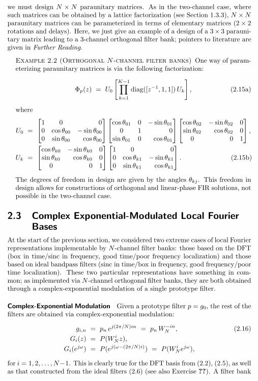
66 Chapter 2. Local Fourier Bases on Sequences
we must design N × N paraunitary matrices. As in the two-channel case, wheresuch matrices can be obtained by a lattice factorization (see Section 1.3.3), N ×Nparaunitary matrices can be parameterized in terms of elementary matrices (2 × 2rotations and delays). Here, we just give an example of a design of a 3× 3 parauni-tary matrix leading to a 3-channel orthogonal filter bank; pointers to literature aregiven in Further Reading.
Example 2.2 (Orthogonal N-channel filter banks) One way of param-eterizing paraunitary matrices is via the following factorization:
Φp(z) = U0
[K−1∏
k=1
diag([z−1, 1, 1])Uk
], (2.15a)
where
U0 =
1 0 00 cos θ00 − sin θ000 sin θ00 cos θ00
cos θ01 0 − sin θ01
0 1 0sin θ01 0 cos θ01
cos θ02 − sin θ02 0sin θ02 cos θ02 0
0 0 1
,
Uk =
cos θk0 − sin θk0 0sin θk0 cos θk0 0
0 0 1
1 0 00 cos θk1 − sin θk10 sin θk1 cos θk1
. (2.15b)
The degrees of freedom in design are given by the angles θkj . This freedom indesign allows for constructions of orthogonal and linear-phase FIR solutions, notpossible in the two-channel case.
2.3 Complex Exponential-Modulated Local FourierBases
At the start of the previous section, we considered two extreme cases of local Fourierrepresentations implementable by N -channel filter banks: those based on the DFT(box in time/sinc in frequency, good time/poor frequency localization) and thosebased on ideal bandpass filters (sinc in time/box in frequency, good frequency/poortime localization). These two particular representations have something in com-mon; as implemented via N -channel orthogonal filter banks, they are both obtainedthrough a complex-exponential modulation of a single prototype filter.
Complex-Exponential Modulation Given a prototype filter p = g0, the rest of thefilters are obtained via complex-exponential modulation:
gi,n = pn ej(2π/N)in = pnW
−inN
, (2.16)
Gi(z) = P (W i
Nz),
Gi(ejω) = P (ej(ω−(2π/N)i)) = P (W i
Nejω),
for i = 1, 2, . . . , N−1. This is clearly true for the DFT basis from (2.2), (2.5), as wellas that constructed from the ideal filters (2.6) (see also Exercise ??). A filter bank

2.3. Complex Exponential-Modulated Local Fourier Bases 67
implementing such an expansion is often called complex exponential-modulated filterbank. While the prototype filter p = g0 is typically real, the rest of the bandpassfilters are complex.
2.3.1 Balian-Low Theorem
We are now back to the question whether we can find complex exponential-modulatedlocal Fourier bases with a trade-off of time and frequency localization we have seenfor the DFT and sinc bases in Figure 2.2. To that end, we might want to worsenthe time localization of the DFT a bit in the hope of improving the frequencyone; unfortunately, the following result excludes the possibility of having complexexponential-modulated local Fourier bases with support longer than N :13
Theorem 2.2 (Discrete Balian-Low theorem) There does not exist a com-plex exponential-modulated local Fourier basis implementable by an N -channelFIR filter bank, except for a filter bank with filters of length N .
Proof. To prove the theorem, we analyze the structure of the polyphase matrix of acomplex exponential-modulated filter bank with filters as in (2.16). Given the polyphaserepresentation (2.12d) of the prototype filter p = g0,
P (z) = P0(zN ) + z−1P1(z
N) + . . .+ z−(N−1)PN−1(zN ),
the modulated versions become
Gi(z) = P (W iNz) = P0(z
N ) +W−iN z−1P1(z
N) + . . .+W−(N−1)iN z−(N−1)PN−1(z
N )
for i = 1, 2, . . . , N − 1. As an example, for N = 3, the polyphase matrix is
Φp(z) =
P0(z) P0(z) P0(z)P1(z) W−1
3 P1(z) W−23 P1(z)
P2(z) W−23 P2(z) W−1
3 P2(z)
=
P0(z)
P1(z)P2(z)
1 1 11 W−1
3 W−23
1 W−23 W−1
3
︸ ︷︷ ︸F∗
, (2.17)
that is, a product of a diagonal matrix of prototype filter polyphase components andthe conjugated DFT matrix (3.161a). According to Theorem 2.1, this filter bank im-plements an FIR biorthogonal expansion if and only if Φp(z) is a monomial. So,
det(Φp(z)) =
N−1∏
j=0
Pj(z) det(F∗)︸ ︷︷ ︸
1/√N
=√N
N−1∏
j=0
Pj(z), (2.18)
13This result is known as the Balian-Low theorem in the continuous-domain setting, see Sec-tion 5.4.1.
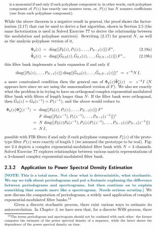
68 Chapter 2. Local Fourier Bases on Sequences
is a monomial if and only if each polyphase component is; in other words, each polyphasecomponent of P (z) has exactly one nonzero term, or, P (z) has N nonzero coefficients(one from each polyphase component).
While the above theorem is a negative result in general, the proof shows the factor-ization (2.17) that can be used to derive a fast algorithm, shown in Section 2.5 (thesame factorization is used in Solved Exercise ?? to derive the relationship betweenthe modulation and polyphase matrices). Rewriting (2.17) for general N , as wellas the analysis polyphase version of it,
Φp(z) = diag([P0(z), P1(z), . . . , PN−1(z)])F∗, (2.19a)
Φp(z) = diag([G0,0(z), G0,1(z), . . . , G0,N−1(z)])F∗, , (2.19b)
this filter bank implements a basis expansion if and only if
diag([P0(z), . . . , PN−1(z)]) diag([G0,0(z), . . . , G0,N−1(z)])∗ = z−kN I,
a more constrained condition then the general one of Φp(z)Φ∗p(z) = z−kI (N
appears here since we are using the unnormalized version of F ). We also see exactlywhat the problem is in trying to have an orthogonal complex exponential-modulatedfilter bank with filters of length longer than N : If the filter bank were orthogonal,then G0(z) = G0(z
−1) = P (z−1), and the above would reduce to
Φp(z)Φ∗p(z−1) = diag([P0(z), P1(z), . . . , PN−1(z)])F
∗
F diag([P0(z−1), P1(z
−1), . . . , PN−1(z−1)])∗
= N diag([P0(z)P0(z−1), P1(z)P1(z
−1), . . . , PN−1(z)PN−1(z−1)])
= N I,
possible with FIR filters if and only if each polyphase component Pj(z) of the proto-type filter P (z) were exactly of length 1 (we assumed the prototype to be real). Fig-ure 2.4 depicts a complex exponential-modulated filter bank with N = 3 channels.Solved Exercise ?? explores relationships between various matrix representations ofa 3-channel complex exponential-modulated filter bank.
2.3.2 Application to Power Spectral Density Estimation
[NOTE: This is a total mess. Not clear what is deterministic, what stochastic.
We say we talk about periodograms and put a footnote explaning the difference
between periodograms and spectrograms, but then continue on to explain
something that sounds more like a spectrogram. Needs serious scrutiny.] Wenow discuss the computation of periodograms, a widely used application of complexexponential-modulated filter banks.14
Given a discrete stochastic process, there exist various ways to estimate itsautocorrelation. In Chapter 3, we have seen that, for a discrete WSS process, there
14The terms periodogram and spectrogram should not be confused with each other: the formercomputes the estimate of the power spectral density of a sequence, while the latter shows thedependence of the power spectral density on time.
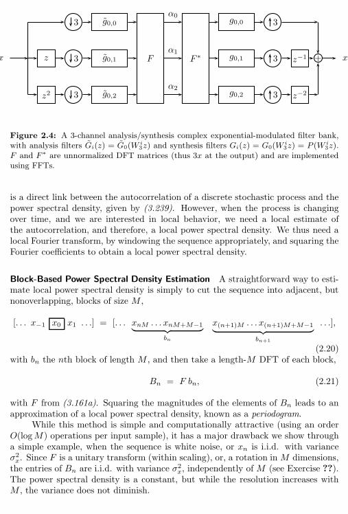
2.3. Complex Exponential-Modulated Local Fourier Bases 69
x
3 g0,0α0
g0,0 3
z 3 g0,1 Fα1
F ∗ g0,1 3 z−1 +
z2 3 g0,2α2
g0,2 3 z−2
x
Figure 2.4: A 3-channel analysis/synthesis complex exponential-modulated filter bank,with analysis filters Gi(z) = G0(W
i3z) and synthesis filters Gi(z) = G0(W
i3z) = P (W i
3z).F and F ∗ are unnormalized DFT matrices (thus 3x at the output) and are implementedusing FFTs.
is a direct link between the autocorrelation of a discrete stochastic process and thepower spectral density, given by (3.239). However, when the process is changingover time, and we are interested in local behavior, we need a local estimate ofthe autocorrelation, and therefore, a local power spectral density. We thus need alocal Fourier transform, by windowing the sequence appropriately, and squaring theFourier coefficients to obtain a local power spectral density.
Block-Based Power Spectral Density Estimation A straightforward way to esti-mate local power spectral density is simply to cut the sequence into adjacent, butnonoverlapping, blocks of size M ,
[. . . x−1 x0 x1 . . .] = [. . . xnM . . . xnM+M−1︸ ︷︷ ︸bn
x(n+1)M . . . x(n+1)M+M−1︸ ︷︷ ︸bn+1
. . .],
(2.20)with bn the nth block of length M , and then take a length-M DFT of each block,
Bn = F bn, (2.21)
with F from (3.161a). Squaring the magnitudes of the elements of Bn leads to anapproximation of a local power spectral density, known as a periodogram.
While this method is simple and computationally attractive (using an orderO(logM) operations per input sample), it has a major drawback we show througha simple example, when the sequence is white noise, or xn is i.i.d. with varianceσ2x. Since F is a unitary transform (within scaling), or, a rotation in M dimensions,
the entries of Bn are i.i.d. with variance σ2x, independently of M (see Exercise ??).
The power spectral density is a constant, but while the resolution increases withM , the variance does not diminish.
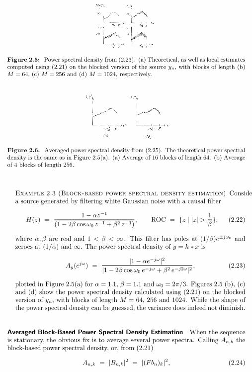
70 Chapter 2. Local Fourier Bases on Sequences
Figure 2.5: Power spectral density from (2.23). (a) Theoretical, as well as local estimatescomputed using (2.21) on the blocked version of the source yn, with blocks of length (b)M = 64, (c) M = 256 and (d) M = 1024, respectively.
Figure 2.6: Averaged power spectral density from (2.25). The theoretical power spectraldensity is the same as in Figure 2.5(a). (a) Average of 16 blocks of length 64. (b) Averageof 4 blocks of length 256.
Example 2.3 (Block-based power spectral density estimation) Considera source generated by filtering white Gaussian noise with a causal filter
H(z) =1− αz−1
(1− 2β cosω0 z−1 + β2 z−1), ROC = z | |z| > 1
β, (2.22)
where α, β are real and 1 < β < ∞. This filter has poles at (1/β)e±jω0 andzeroes at (1/α) and ∞. The power spectral density of y = h ∗ x is
Ay(ejω) =
|1− αe−jω |2|1− 2β cosω0 e−jω + β2 e−j2ω|2 , (2.23)
plotted in Figure 2.5(a) for α = 1.1, β = 1.1 and ω0 = 2π/3. Figures 2.5 (b), (c)and (d) show the power spectral density calculated using (2.21) on the blockedversion of yn, with blocks of length M = 64, 256 and 1024. While the shape ofthe power spectral density can be guessed, the variance does indeed not diminish.
Averaged Block-Based Power Spectral Density Estimation When the sequenceis stationary, the obvious fix is to average several power spectra. Calling An,k theblock-based power spectral density, or, from (2.21)
An,k = |Bn,k|2 = |(Fbn)k|2, (2.24)
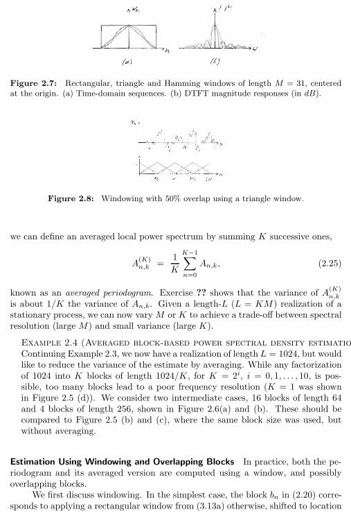
2.3. Complex Exponential-Modulated Local Fourier Bases 71
Figure 2.7: Rectangular, triangle and Hamming windows of length M = 31, centeredat the origin. (a) Time-domain sequences. (b) DTFT magnitude responses (in dB).
Figure 2.8: Windowing with 50% overlap using a triangle window.
we can define an averaged local power spectrum by summing K successive ones,
A(K)n,k
=1
K
K−1∑
n=0
An,k, (2.25)
known as an averaged periodogram. Exercise ?? shows that the variance of A(K)n,k
is about 1/K the variance of An,k. Given a length-L (L = KM) realization of astationary process, we can now varyM or K to achieve a trade-off between spectralresolution (large M) and small variance (large K).
Example 2.4 (Averaged block-based power spectral density estimation)Continuing Example 2.3, we now have a realization of length L = 1024, but wouldlike to reduce the variance of the estimate by averaging. While any factorizationof 1024 into K blocks of length 1024/K, for K = 2i, i = 0, 1, . . . , 10, is pos-sible, too many blocks lead to a poor frequency resolution (K = 1 was shownin Figure 2.5 (d)). We consider two intermediate cases, 16 blocks of length 64and 4 blocks of length 256, shown in Figure 2.6(a) and (b). These should becompared to Figure 2.5 (b) and (c), where the same block size was used, butwithout averaging.
Estimation Using Windowing and Overlapping Blocks In practice, both the pe-riodogram and its averaged version are computed using a window, and possiblyoverlapping blocks.
We first discuss windowing. In the simplest case, the block bn in (2.20) corre-sponds to applying a rectangular window from (3.13a) otherwise, shifted to location
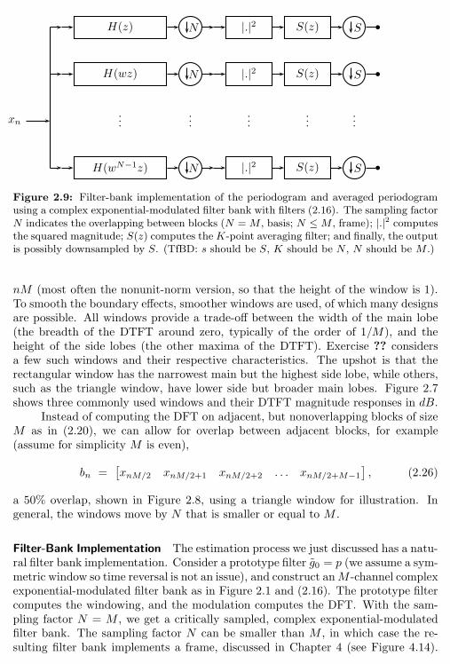
72 Chapter 2. Local Fourier Bases on Sequences
xn
H(z) N
H(wz) N
H(wN−1z) N
......
|.|2 S(z) S
|.|2 S(z) S
......
...
|.|2 S(z) S
Figure 2.9: Filter-bank implementation of the periodogram and averaged periodogramusing a complex exponential-modulated filter bank with filters (2.16). The sampling factorN indicates the overlapping between blocks (N =M , basis; N ≤M , frame); |.|2 computesthe squared magnitude; S(z) computes theK-point averaging filter; and finally, the outputis possibly downsampled by S. (TfBD: s should be S, K should be N , N should be M .)
nM (most often the nonunit-norm version, so that the height of the window is 1).To smooth the boundary effects, smoother windows are used, of which many designsare possible. All windows provide a trade-off between the width of the main lobe(the breadth of the DTFT around zero, typically of the order of 1/M), and theheight of the side lobes (the other maxima of the DTFT). Exercise ?? considersa few such windows and their respective characteristics. The upshot is that therectangular window has the narrowest main but the highest side lobe, while others,such as the triangle window, have lower side but broader main lobes. Figure 2.7shows three commonly used windows and their DTFT magnitude responses in dB.
Instead of computing the DFT on adjacent, but nonoverlapping blocks of sizeM as in (2.20), we can allow for overlap between adjacent blocks, for example(assume for simplicity M is even),
bn =[xnM/2 x
nM/2+1 xnM/2+2 . . . x
nM/2+M−1
], (2.26)
a 50% overlap, shown in Figure 2.8, using a triangle window for illustration. Ingeneral, the windows move by N that is smaller or equal to M .
Filter-Bank Implementation The estimation process we just discussed has a natu-ral filter bank implementation. Consider a prototype filter g0 = p (we assume a sym-metric window so time reversal is not an issue), and construct anM -channel complexexponential-modulated filter bank as in Figure 2.1 and (2.16). The prototype filtercomputes the windowing, and the modulation computes the DFT. With the sam-pling factor N = M , we get a critically sampled, complex exponential-modulatedfilter bank. The sampling factor N can be smaller than M , in which case the re-sulting filter bank implements a frame, discussed in Chapter 4 (see Figure 4.14).
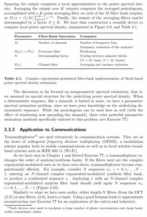
2.3. Complex Exponential-Modulated Local Fourier Bases 73
Squaring the output computes a local approximation to the power spectral den-sity. Averaging the output over K outputs computes the averaged periodogram,accomplished with a K-point averaging filter on each of the M filter bank outputs,or S(z) = (1/K)
∑K−1m=0 z
−m. Finally, the output of the averaging filters maybedownsampled by a factor S ≤ K. We have thus constructed a versatile device tocompute local power spectral density, summarized in Figure 2.9, and Table 2.1.
Parameter Filter-Bank Operation Computes
M Number of channels Number of frequency bins
(frequency resolution of the analysis)
G0(z) = P (z) Prototype filter Windowing
N Downsampling factor Overlap between adjacent blocks
(N = M , basis; N < M , frame)
S(z) Channel filter Averaging and variance reduction
Table 2.1: Complex exponential-modulated filter-bank implementation of block-basedpower spectral density estimation.
The discussion so far focused on nonparametric spectral estimation, that is,we assumed no special structure for the underlying power spectral density. Whena deterministic sequence, like a sinusoid, is buried in noise, we have a parametricspectral estimation problem, since we have prior knowledge on the underlying de-terministic sequence. While the periodogram can be used here as well (with theeffect of windowing now spreading the sinusoid), there exist powerful parametricestimation methods specifically tailored to this problem (see Exercise ??).
2.3.3 Application to Communications
Transmultiplexers15 are used extensively in communication systems. They are atthe heart of orthogonal frequency division multiplexing (OFDM), a modulationscheme popular both in mobile communications as well as in local wireless broad-band systems such as IEEE 802.11 (Wi-Fi).
As we have seen in Chapter 1 and Solved Exercise ??, a transmultiplexer ex-changes the order of analysis/synthesis banks. If the filters used are the complexexponential-modulated ones as we have seen above, transmultiplexers become com-putationally efficient. For example, consider N sequences αi, i = 0, 1, . . . , N −1, entering an N -channel complex exponential-modulated synthesis filter bank,to produce a synthesized sequence x. Analyzing x with an N -channel complexexponential-modulated analysis filter bank should yield again N sequences αi,i = 0, 1, . . . , N − 1 (Figure 2.10).
Similarly to what we have seen earlier, either length-N filters (from the DFT(2.2)) or sinc filters, (2.6), lead to a basis. Using a good lowpass leads to approximatereconstruction (see Exercise ?? for an exploration of the end-to-end behavior).
15Such devices were used to modulate a large number of phone conversations onto large band-width transatlantic cables.
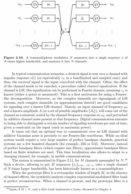
74 Chapter 2. Local Fourier Bases on Sequences
α0
α1
αN−1
......
N g0
N g1
N gN−1
... +x
g0 N
g1 N
gN−1 N
......
...
α0
α1
αN−1
Figure 2.10: A transmultiplexer modulates N sequences into a single sequence x ofN-times higher bandwidth, and analyzes it into N channels.
In typical communication scenarios, a desired signal is sent over a channel withimpulse response c(t) (or equivalently cn in a bandlimited and sampled case), andthus, the received signal is the input convolved with the channel. Often, the effectof the channel needs to be canceled, a procedure called channel equalization. If thechannel is LSI, this equalization can be performed in Fourier domain, assuming cn isknown (either a priori or measured). This is a first motivation for using a Fourier-like decomposition. Moreover, as the complex sinusoids are eigensignals of LSIsystems, such complex sinusoids (or approximations thereof) are good candidatesfor signaling over a known LSI channel. Namely, an input sinusoid of frequency ω0
and a known amplitude A (or a set of possible amplitudes Ai), will come out of thechannel as a sinusoid, scaled by the channel frequency response at ω0, and perturbedby additive channel noise present at that frequency. Digital communication amountsto being able to distinguish a certain number of signaling waveforms per unit of time,given a constraint on the input (such as maximum power).
It turns out that an optimal way to communicate over an LSI channel withadditive Gaussian noise is precisely to use Fourier-like waveforms. While an idealsystem would require a very large number of perfect bandpass channels, practicalsystems use a few hundred channels (for example, 256 or 512). Moreover, insteadof perfect bandpass filters (which require sinc filters), approximate bandpass filtersbased on finite windows are used. This time localization also allows to adapt to achanging channel, for example, in mobile communications.
The system is summarized in Figure 2.11, for M channels upsampled by N .16
Such a device, allowing to put M sequences xii=0,...,M−1, onto a single channelof N -times larger bandwidth, has been historically known as a transmultiplexer.
When the prototype filter is a rectangular window of lengthM , in the absenceof channel effects, the synthesis/analysis complex exponential-modulated filter bankis perfect reconstruction. When a channel is present, and the prototype filter is a
16Again, if M > N , such a filter bank implements a frame, discussed in Chapter 4.
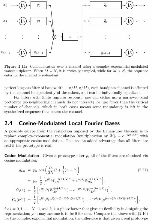
2.4. Cosine-Modulated Local Fourier Bases 75
x0
x1
xM−1
......
N g0
N g1
N gM−1
... + c
g0 N
g1 N
gM−1 N
......
Figure 2.11: Communication over a channel using a complex exponential-modulatedtransmultiplexer. When M = N , it is critically sampled, while for M > N , the sequenceentering the channel is redundant.
perfect lowpass filter of bandwidth [−π/M, π/M), each bandpass channel is affectedby the channel independently of the others, and can be individually equalized.
For filters with finite impulse response, one can either use a narrower-bandprototype (so neighboring channels do not interact), or, use fewer than the criticalnumber of channels, which in both cases means some redundancy is left in thesynthesized sequence that enters the channel.
2.4 Cosine-Modulated Local Fourier Bases
A possible escape from the restriction imposed by the Balian-Low theorem is toreplace complex-exponential modulation (multiplication by W i
N= e−j2πi/N ) with
an appropriate cosine modulation. This has an added advantage that all filters arereal if the prototype is real.
Cosine Modulation Given a prototype filter p, all of the filters are obtained viacosine modulation:
gi,n = pn cos
(2π
2N(i +
1
2)n+ θi
)(2.27)
= pn1
2
[ejθiW
−(i+1/2)n2N + e−jθiW (i+1/2)n
2N
],
Gi(z) =1
2
[ejθiP (W
(i+1/2)2N z) + e−jθiP (W−(i+1/2)
2N z)],
Gi(ejω) =
1
2
[ejθiP (ej(ω−(2π/2N)(i+1/2))) + e−jθiP (ej(ω+(2π/2N)(i+1/2))
],
for i = 0, 1, . . . , N−1, and θi is a phase factor that gives us flexibility in designing therepresentation; you may assume it to be 0 for now. Compare the above with (2.16)for the complex-exponential modulation; the difference is that given a real prototype
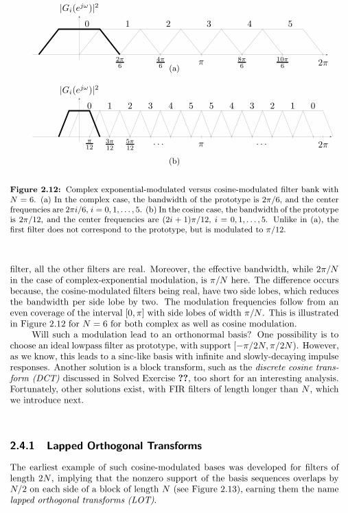
76 Chapter 2. Local Fourier Bases on Sequences
2π6
4π6
π 8π6
10π6 2π
0 1 2 3 4 5
|Gi(ejω)|2
(a)
0 1 2 3 4 5 5 4 3 2 1 0
π
123π12
5π12
· · · · · ·π 2π
|Gi(ejω)|2
(b)
Figure 2.12: Complex exponential-modulated versus cosine-modulated filter bank withN = 6. (a) In the complex case, the bandwidth of the prototype is 2π/6, and the centerfrequencies are 2πi/6, i = 0, 1, . . . , 5. (b) In the cosine case, the bandwidth of the prototypeis 2π/12, and the center frequencies are (2i + 1)π/12, i = 0, 1, . . . , 5. Unlike in (a), thefirst filter does not correspond to the prototype, but is modulated to π/12.
filter, all the other filters are real. Moreover, the effective bandwidth, while 2π/Nin the case of complex-exponential modulation, is π/N here. The difference occursbecause, the cosine-modulated filters being real, have two side lobes, which reducesthe bandwidth per side lobe by two. The modulation frequencies follow from aneven coverage of the interval [0, π] with side lobes of width π/N . This is illustratedin Figure 2.12 for N = 6 for both complex as well as cosine modulation.
Will such a modulation lead to an orthonormal basis? One possibility is tochoose an ideal lowpass filter as prototype, with support [−π/2N, π/2N). However,as we know, this leads to a sinc-like basis with infinite and slowly-decaying impulseresponses. Another solution is a block transform, such as the discrete cosine trans-form (DCT) discussed in Solved Exercise ??, too short for an interesting analysis.Fortunately, other solutions exist, with FIR filters of length longer than N , whichwe introduce next.
2.4.1 Lapped Orthogonal Transforms
The earliest example of such cosine-modulated bases was developed for filters oflength 2N , implying that the nonzero support of the basis sequences overlaps byN/2 on each side of a block of length N (see Figure 2.13), earning them the namelapped orthogonal transforms (LOT).
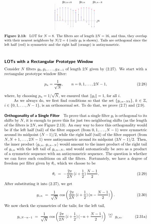
2.4. Cosine-Modulated Local Fourier Bases 77
8 16
g0,n+8 g0,n g0,n−8
n
Figure 2.13: LOT for N = 8. The filters are of length 2N = 16, and thus, they overlapwith their nearest neighbors by N/2 = 4 (only g0 is shown). Tails are orthogonal since theleft half (red) is symmetric and the right half (orange) is antisymmetric.
LOTs with a Rectangular Prototype Window
Consider N filters g0, g1, . . . , gN−1 of length 2N given by (2.27). We start with arectangular prototype window filter:
pn =1√N, n = 0, 1, . . . , 2N − 1, (2.28)
where, by choosing pn = 1/√N , we ensured that ‖gi‖ = 1, for all i.
As we always do, we first find conditions so that the set gi,n−Nk, k ∈ Z,i ∈ 0, 1, . . . , N − 1, is an orthonormal set. To do that, we prove (2.7) and (2.9).
Orthogonality of a Single Filter To prove that a single filter gi is orthogonal to itsshifts by N , it is enough to prove this for just two neighboring shifts (as the lengthof the filters is 2N , see Figure 2.13). An easy way to force this orthogonality wouldbe if the left half (tail) of the filter support (from 0, 1, . . . , N − 1) were symmetricaround its midpoint (N − 1)/2, while the right half (tail) of the filter support (fromN,N + 1, . . . , 2N − 1) were antisymmetric around its midpoint (3N − 1)/2. Then,the inner product 〈gi,n, gi,n−N 〉 would amount to the inner product of the right tailof gi,n with the left tail of gi,n−N , and would automatically be zero as a productof a symmetric sequence with an antisymmetric sequence. The question is whetherwe can force such conditions on all the filters. Fortunately, we have a degree offreedom per filter given by θi, which we choose to be
θi = − 2π
2N(i +
1
2)N − 1
2. (2.29)
After substituting it into (2.27), we get
gi,n =1√N
cos
(2π
2N(i+
1
2) (n− N − 1
2)
). (2.30)
We now check the symmetries of the tails; for the left tail,
gi,N−n−1 =1√N
cos
(2π
2N(i+
1
2) (−n+
N − 1
2)
)(a)= gi,n, (2.31a)
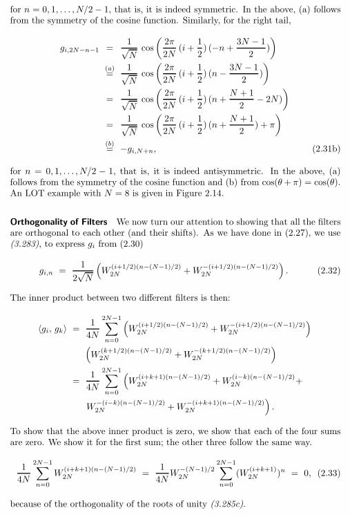
78 Chapter 2. Local Fourier Bases on Sequences
for n = 0, 1, . . . , N/2− 1, that is, it is indeed symmetric. In the above, (a) followsfrom the symmetry of the cosine function. Similarly, for the right tail,
gi,2N−n−1 =1√N
cos
(2π
2N(i+
1
2) (−n+
3N − 1
2)
)
(a)=
1√N
cos
(2π
2N(i+
1
2) (n− 3N − 1
2)
)
=1√N
cos
(2π
2N(i+
1
2) (n+
N + 1
2− 2N)
)
=1√N
cos
(2π
2N(i+
1
2) (n+
N + 1
2) + π
)
(b)= −gi,N+n, (2.31b)
for n = 0, 1, . . . , N/2 − 1, that is, it is indeed antisymmetric. In the above, (a)follows from the symmetry of the cosine function and (b) from cos(θ+ π) = cos(θ).An LOT example with N = 8 is given in Figure 2.14.
Orthogonality of Filters We now turn our attention to showing that all the filtersare orthogonal to each other (and their shifts). As we have done in (2.27), we use(3.283), to express gi from (2.30)
gi,n =1
2√N
(W
(i+1/2)(n−(N−1)/2)2N +W
−(i+1/2)(n−(N−1)/2)2N
). (2.32)
The inner product between two different filters is then:
〈gi, gk〉 =1
4N
2N−1∑
n=0
(W
(i+1/2)(n−(N−1)/2)2N +W
−(i+1/2)(n−(N−1)/2)2N
)
(W
(k+1/2)(n−(N−1)/2)2N +W
−(k+1/2)(n−(N−1)/2)2N
)
=1
4N
2N−1∑
n=0
(W
(i+k+1)(n−(N−1)/2)2N +W
(i−k)(n−(N−1)/2)2N +
W−(i−k)(n−(N−1)/2)2N +W
−(i+k+1)(n−(N−1)/2)2N
).
To show that the above inner product is zero, we show that each of the four sumsare zero. We show it for the first sum; the other three follow the same way.
1
4N
2N−1∑
n=0
W(i+k+1)(n−(N−1)/2)2N =
1
4NW
−(N−1)/22N
2N−1∑
n=0
(W(i+k+1)2N )n = 0, (2.33)
because of the orthogonality of the roots of unity (3.285c).

2.4. Cosine-Modulated Local Fourier Bases 79
nn
nnn
nnn
g0,n g1,n g2,n
g3,n g4,n g5,n
g6,n g7,n
ω
|Gi(ejω)|
Figure 2.14: LOT for N = 8 with a rectangular prototype window. The eight basissequences (note the symmetric and antisymmetric tails) and their magnitude responses,showing the uniform split of the spectrum.
Matrix View As usual, we find the matrix view of an expansion to be illuminating.We can write the output of an LOT synthesis bank similarly to (1.7),
Φ =
. . .
G0
G1 G0
G1 G0
G1
. . .
, (2.34)
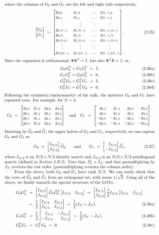
80 Chapter 2. Local Fourier Bases on Sequences
where the columns of G0 and G1 are the left and right tails respectively,
[G0
G1
]=
g0,0 g1,0 . . . gN−1,0
g0,1 g1,1 . . . gN−1,1
......
. . ....
g0,N−1 g1,N−1 . . . gN−1,N−1
g0,N g1,N . . . gN−1,N
g0,N+1 g1,N+1 . . . gN−1,N+1
......
. . ....
g0,2N−1 g1,2N−1 . . . gN−1,2N−1
. (2.35)
Since the expansion is orthonormal, ΦΦT = I, but also ΦTΦ = I, or,
G0GT
0 +G1GT
1 = I, (2.36a)
G1GT
0 = G0GT
1 = 0, (2.36b)
GT0G0 +GT1 G1 = I, (2.36c)
GT0G1 = GT1 G0 = 0. (2.36d)
Following the symmetry/antisymmetry of the tails, the matrices G0 and G1 haverepeated rows. For example, for N = 4,
G0 =
g0,0 g1,0 g2,0 g3,0g0,1 g1,1 g2,1 g3,1g0,1 g1,1 g2,1 g3,1g0,0 g1,0 g2,0 g3,0
and G1 =
g0,4 g1,4 g2,4 g3,4g0,5 g1,5 g2,5 g3,5−g0,5 −g1,5 −g2,5 −g3,5−g0,4 −g1,4 −g2,4 −g3,4
.
Denoting by G0 and G1 the upper halves of G0 and G1, respectively, we can expressG0 and G1 as
G0 =
[IN/2
JN/2
]G0 and G1 =
[IN/2
−JN/2
]G1, (2.37)
where IN/2 is an N/2×N/2 identity matrix and J
N/2 is an N/2×N/2 antidiagonalmatrix (defined in Section 2.B.2). Note that J2
N= IN , and that premultiplying by
JN reverses the row order (postmultiplying reverses the column order).From the above, both G0 and G1 have rank N/2. We can easily check that
the rows of G0 and G1 form an orthogonal set, with norm 1/√2. Using all of the
above, we finally unearth the special structure of the LOTs:
G0GT
0 =
[IN/2
JN/2
]G0G
T
0
[IN/2 J
N/2
]=
[IN/2
JN/2
]1
2IN/2
[IN/2 J
N/2
]
=1
2
[IN/2 J
N/2
JN/2 I
N/2
]=
1
2(IN + JN ), (2.38a)
G1GT
1 =1
2
[IN/2 −J
N/2
−JN/2 I
N/2
]=
1
2(IN − JN ), (2.38b)
GT0 G1 = GT1G0 = 0. (2.38c)
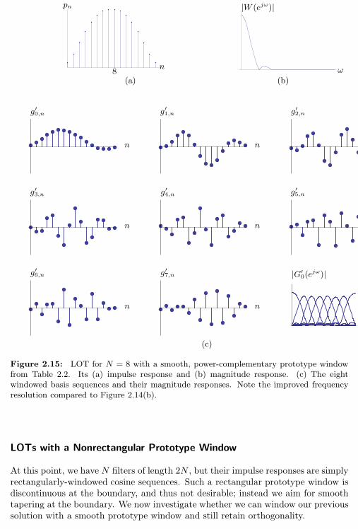
2.4. Cosine-Modulated Local Fourier Bases 81
n
pn
8
|W (ejω)|
ω
(a) (b)
nn
nnn
nnn
g′0,n g′1,n g′2,n
g′3,n g′4,n g′5,n
g′6,n g′7,n
ω
|G′0(e
jω)|
(c)
Figure 2.15: LOT for N = 8 with a smooth, power-complementary prototype windowfrom Table 2.2. Its (a) impulse response and (b) magnitude response. (c) The eightwindowed basis sequences and their magnitude responses. Note the improved frequencyresolution compared to Figure 2.14(b).
LOTs with a Nonrectangular Prototype Window
At this point, we have N filters of length 2N , but their impulse responses are simplyrectangularly-windowed cosine sequences. Such a rectangular prototype window isdiscontinuous at the boundary, and thus not desirable; instead we aim for smoothtapering at the boundary. We now investigate whether we can window our previoussolution with a smooth prototype window and still retain orthogonality.
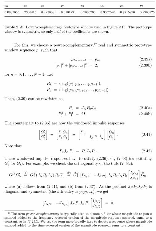
82 Chapter 2. Local Fourier Bases on Sequences
p0 p1 p2 p3 p4 p5 p6 p7
0.0887655 2366415 0.4238081 0.6181291 0.7860766 0.9057520 0.9715970 0.9960525
Table 2.2: Power-complementary prototype window used in Figure 2.15. The prototypewindow is symmetric, so only half of the coefficients are shown.
For this, we choose a power-complementary,17 real and symmetric prototypewindow sequence p, such that:
p2N−n−1 = pn, (2.39a)
|pn|2 + |pN−n−1|2 = 2, (2.39b)
for n = 0, 1, . . . , N − 1. Let
P0 = diag([p0, p1, . . . , pN−1]),
P1 = diag([pN , pN+1, . . . , p2N−1]).
Then, (2.39) can be rewritten as
P1 = JNP0JN , (2.40a)
P 20 + P 2
1 = 2I. (2.40b)
The counterpart to (2.35) are now the windowed impulse responses
[G′
0
G′1
]=
[P0G0
P1G1
]=
[P0
JNP0JN
] [G0
G1
]. (2.41)
Note thatP0JNP0 = P1JNP1. (2.42)
These windowed impulse responses have to satisfy (2.36), or, (2.38) (substitutingG′ifor Gi). For example, we check the orthogonality of the tails (2.38c):
G′T1 G
′0
(a)= GT1 (JNP0JN )P0G0
(b)= GT1
[IN/2 −J
N/2
]JNP0JNP0
[IN/2
JN/2
]G0,
where (a) follows from (2.41), and (b) from (2.37). As the product JNP0JNP0 isdiagonal and symmetric (the kth entry is pkpN−k), we get
[IN/2 −J
N/2
]JNP0JNP0
[IN/2
JN/2
]= 0.
17The term power complementary is typically used to denote a filter whose magnitude responsesquared added to the frequency-reversed version of the magnitude response squared, sums to aconstant, as in (3.214). We use the term more broadly here to denote a sequence whose magnitudesquared added to the time-reversed version of the magnitude squared, sums to a constant.
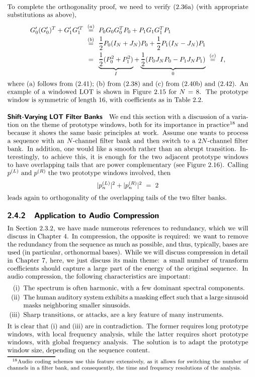
2.4. Cosine-Modulated Local Fourier Bases 83
To complete the orthogonality proof, we need to verify (2.36a) (with appropriatesubstitutions as above),
G′0(G
′0)T +G′
1G′T1
(a)= P0G0G
T
0 P0 + P1G1GT
1 P1
(b)=
1
2P0(IN + JN )P0 +
1
2P1(IN − JN )P1
=1
2(P 2
0 + P 21 )
︸ ︷︷ ︸I
+1
2(P0JNP0 − P1JNP1)︸ ︷︷ ︸
0
(c)= I,
where (a) follows from (2.41); (b) from (2.38) and (c) from (2.40b) and (2.42). Anexample of a windowed LOT is shown in Figure 2.15 for N = 8. The prototypewindow is symmetric of length 16, with coefficients as in Table 2.2.
Shift-Varying LOT Filter Banks We end this section with a discussion of a varia-tion on the theme of prototype windows, both for its importance in practice18 andbecause it shows the same basic principles at work. Assume one wants to processa sequence with an N -channel filter bank and then switch to a 2N -channel filterbank. In addition, one would like a smooth rather than an abrupt transition. In-terestingly, to achieve this, it is enough for the two adjacent prototype windowsto have overlapping tails that are power complementary (see Figure 2.16). Callingp(L) and p(R) the two prototype windows involved, then
|p(L)n|2 + |p(R)
n|2 = 2
leads again to orthogonality of the overlapping tails of the two filter banks.
2.4.2 Application to Audio Compression
In Section 2.3.2, we have made numerous references to redundancy, which we willdiscuss in Chapter 4. In compression, the opposite is required: we want to removethe redundancy from the sequence as much as possible, and thus, typically, bases areused (in particular, orthonormal bases). While we will discuss compression in detailin Chapter 7, here, we just discuss its main theme: a small number of transformcoefficients should capture a large part of the energy of the original sequence. Inaudio compression, the following characteristics are important:
(i) The spectrum is often harmonic, with a few dominant spectral components.
(ii) The human auditory system exhibits a masking effect such that a large sinusoidmasks neighboring smaller sinusoids.
(iii) Sharp transitions, or attacks, are a key feature of many instruments.
It is clear that (i) and (iii) are in contradiction. The former requires long prototypewindows, with local frequency analysis, while the latter requires short prototypewindows, with global frequency analysis. The solution is to adapt the prototypewindow size, depending on the sequence content.
18Audio coding schemes use this feature extensively, as it allows for switching the number ofchannels in a filter bank, and consequently, the time and frequency resolutions of the analysis.
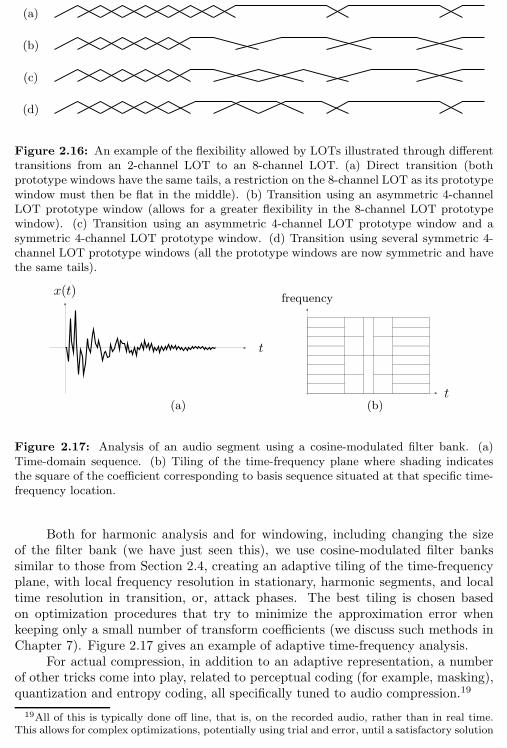
84 Chapter 2. Local Fourier Bases on Sequences
(a)
(b)
(c)
(d)
Figure 2.16: An example of the flexibility allowed by LOTs illustrated through differenttransitions from an 2-channel LOT to an 8-channel LOT. (a) Direct transition (bothprototype windows have the same tails, a restriction on the 8-channel LOT as its prototypewindow must then be flat in the middle). (b) Transition using an asymmetric 4-channelLOT prototype window (allows for a greater flexibility in the 8-channel LOT prototypewindow). (c) Transition using an asymmetric 4-channel LOT prototype window and asymmetric 4-channel LOT prototype window. (d) Transition using several symmetric 4-channel LOT prototype windows (all the prototype windows are now symmetric and havethe same tails).
x(t)
t
frequency
t(a) (b)
Figure 2.17: Analysis of an audio segment using a cosine-modulated filter bank. (a)Time-domain sequence. (b) Tiling of the time-frequency plane where shading indicatesthe square of the coefficient corresponding to basis sequence situated at that specific time-frequency location.
Both for harmonic analysis and for windowing, including changing the sizeof the filter bank (we have just seen this), we use cosine-modulated filter bankssimilar to those from Section 2.4, creating an adaptive tiling of the time-frequencyplane, with local frequency resolution in stationary, harmonic segments, and localtime resolution in transition, or, attack phases. The best tiling is chosen basedon optimization procedures that try to minimize the approximation error whenkeeping only a small number of transform coefficients (we discuss such methods inChapter 7). Figure 2.17 gives an example of adaptive time-frequency analysis.
For actual compression, in addition to an adaptive representation, a numberof other tricks come into play, related to perceptual coding (for example, masking),quantization and entropy coding, all specifically tuned to audio compression.19
19All of this is typically done off line, that is, on the recorded audio, rather than in real time.This allows for complex optimizations, potentially using trial and error, until a satisfactory solution
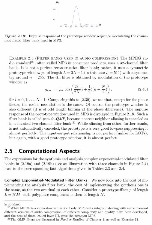
2.5. Computational Aspects 85
64 128 192 256 320 384 448 512
0.01
0.03
n
pn
Figure 2.18: Impulse response of the prototype window sequence modulating the cosine-modulated filter bank used in MP3.
Example 2.5 (Filter banks used in audio compression) The MPEG au-dio standard20, often called MP3 in consumer products, uses a 32-channel filterbank. It is not a perfect reconstruction filter bank; rather, it uses a symmetricprototype window pn of length L = 2N−1 (in this case L = 511) with a symme-try around n = 255. The ith filter is obtained by modulation of the prototypewindow as
gi,n = pn cos
(2π
2N(i+
1
2)(n+
N
2)
), (2.43)
for i = 0, 1, . . . , N−1. Comparing this to (2.30), we see that, except for the phasefactor, the cosine modulation is the same. Of course, the prototype window isalso different (it is of odd length hinting at the phase difference). The impulseresponse of the prototype window used in MP3 is displayed in Figure 2.18. Such afilter bank is called pseudo-QMF, because nearest neighbor aliasing is canceled asin a classical two-channel filter bank.21 While aliasing from other, further bands,is not automatically canceled, the prototype is a very good lowpass suppressing italmost perfectly. The input-output relationship is not perfect (unlike for LOTs),but again, with a good prototype window, it is almost perfect.
2.5 Computational Aspects
The expressions for the synthesis and analysis complex exponential-modulated filterbanks in (2.19a) and (2.19b) (see an illustration with three channels in Figure 2.4)lead to the corresponding fast algorithms given in Tables 2.3 and 2.4.
Complex Exponential-Modulated Filter Banks We now look into the cost of im-plementing the analysis filter bank; the cost of implementing the synthesis one isthe same, as the two are dual to each other. Consider a prototype filter p of lengthL = NM ; each polyphase component is then of length N .
is obtained.20While MPEG is a video standardization body, MP3 is its subgroup dealing with audio. Several
different versions of audio compression, of different complexity and quality, have been developed,and the best of these, called layer III, gave the acronym MP3.
21The QMF filters are discussed in Further Reading of Chapter 1, as well as Exercise ??.
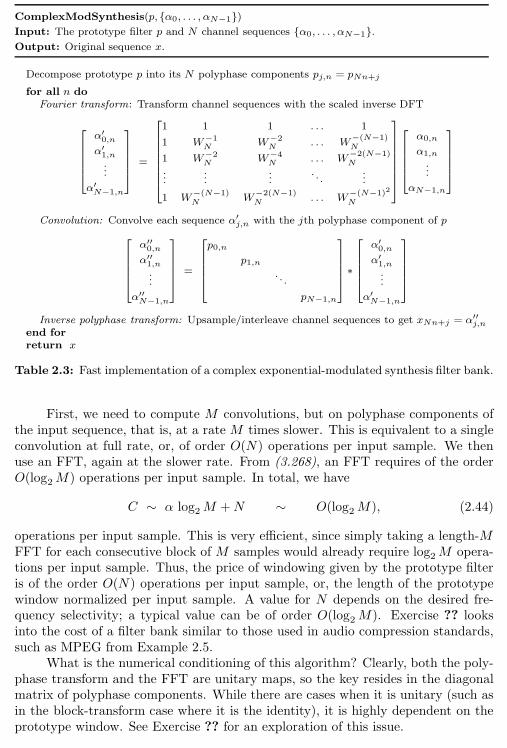
86 Chapter 2. Local Fourier Bases on Sequences
ComplexModSynthesis(p, α0, . . . , αN−1)Input: The prototype filter p and N channel sequences α0, . . . , αN−1.Output: Original sequence x.
Decompose prototype p into its N polyphase components pj,n = pNn+j
for all n doFourier transform: Transform channel sequences with the scaled inverse DFT
α′0,n
α′1,n...
α′N−1,n
=
1 1 1 . . . 1
1 W−1N W−2
N . . . W−(N−1)N
1 W−2N W−4
N . . . W−2(N−1)N
......
.... . .
...
1 W−(N−1)N W
−2(N−1)N . . . W
−(N−1)2
N
α0,n
α1,n
...
αN−1,n
Convolution: Convolve each sequence α′j,n with the jth polyphase component of p
α′′0,n
α′′1,n...
α′′N−1,n
=
p0,n
p1,n. . .
pN−1,n
∗
α′0,n
α′1,n...
α′N−1,n
Inverse polyphase transform: Upsample/interleave channel sequences to get xNn+j = α′′j,n
end forreturn x
Table 2.3: Fast implementation of a complex exponential-modulated synthesis filter bank.
First, we need to compute M convolutions, but on polyphase components ofthe input sequence, that is, at a rate M times slower. This is equivalent to a singleconvolution at full rate, or, of order O(N) operations per input sample. We thenuse an FFT, again at the slower rate. From (3.268), an FFT requires of the orderO(log2M) operations per input sample. In total, we have
C ∼ α log2M +N ∼ O(log2M), (2.44)
operations per input sample. This is very efficient, since simply taking a length-MFFT for each consecutive block of M samples would already require log2M opera-tions per input sample. Thus, the price of windowing given by the prototype filteris of the order O(N) operations per input sample, or, the length of the prototypewindow normalized per input sample. A value for N depends on the desired fre-quency selectivity; a typical value can be of order O(log2M). Exercise ?? looksinto the cost of a filter bank similar to those used in audio compression standards,such as MPEG from Example 2.5.
What is the numerical conditioning of this algorithm? Clearly, both the poly-phase transform and the FFT are unitary maps, so the key resides in the diagonalmatrix of polyphase components. While there are cases when it is unitary (such asin the block-transform case where it is the identity), it is highly dependent on theprototype window. See Exercise ?? for an exploration of this issue.
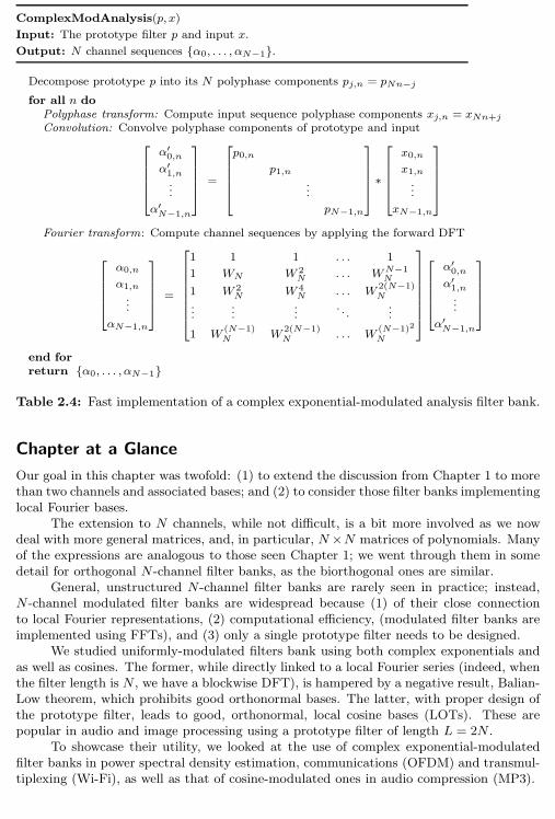
Chapter at a Glance 87
ComplexModAnalysis(p, x)
Input: The prototype filter p and input x.
Output: N channel sequences α0, . . . , αN−1.
Decompose prototype p into its N polyphase components pj,n = pNn−j
for all n doPolyphase transform: Compute input sequence polyphase components xj,n = xNn+jConvolution: Convolve polyphase components of prototype and input
α′0,n
α′1,n...
α′N−1,n
=
p0,n
p1,n...
pN−1,n
∗
x0,n
x1,n...
xN−1,n
Fourier transform: Compute channel sequences by applying the forward DFT
α0,n
α1,n
...
αN−1,n
=
1 1 1 . . . 1
1 WN W 2N . . . WN−1
N
1 W 2N W 4
N . . . W2(N−1)N
......
.... . .
...
1 W(N−1)N W
2(N−1)N . . . W
(N−1)2
N
α′0,n
α′1,n...
α′N−1,n
end forreturn α0, . . . , αN−1
Table 2.4: Fast implementation of a complex exponential-modulated analysis filter bank.
Chapter at a Glance
Our goal in this chapter was twofold: (1) to extend the discussion from Chapter 1 to morethan two channels and associated bases; and (2) to consider those filter banks implementinglocal Fourier bases.
The extension to N channels, while not difficult, is a bit more involved as we nowdeal with more general matrices, and, in particular, N×N matrices of polynomials. Manyof the expressions are analogous to those seen Chapter 1; we went through them in somedetail for orthogonal N-channel filter banks, as the biorthogonal ones are similar.
General, unstructured N-channel filter banks are rarely seen in practice; instead,N-channel modulated filter banks are widespread because (1) of their close connectionto local Fourier representations, (2) computational efficiency, (modulated filter banks areimplemented using FFTs), and (3) only a single prototype filter needs to be designed.
We studied uniformly-modulated filters bank using both complex exponentials andas well as cosines. The former, while directly linked to a local Fourier series (indeed, whenthe filter length is N , we have a blockwise DFT), is hampered by a negative result, Balian-Low theorem, which prohibits good orthonormal bases. The latter, with proper design ofthe prototype filter, leads to good, orthonormal, local cosine bases (LOTs). These arepopular in audio and image processing using a prototype filter of length L = 2N .
To showcase their utility, we looked at the use of complex exponential-modulatedfilter banks in power spectral density estimation, communications (OFDM) and transmul-tiplexing (Wi-Fi), as well as that of cosine-modulated ones in audio compression (MP3).
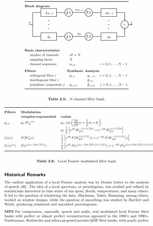
88 Chapter 2. Local Fourier Bases on Sequences
Block diagram
x
gN−1
g0
b
b
b
N
N
αN−1
α0
N
N
gN−1
g0
b
b
b
+x
Basic characteristics
number of channels M = N
sampling factor N
channel sequences αi,n i = 0, 1, . . . , N − 1
Filters Synthesis Analysis
orthogonal filter i gi,n gi,−n i = 0, 1, . . . , N − 1
biorthogonal filter i gi,n
polyphase component j gi,j,n gi,j,n j = 0, 1, . . . , N − 1
Table 2.5: N-channel filter bank.
Filters Modulation
complex-exponential cosine
gi,n pnW−inN pn cos
(2π
2N(i+
1
2)n+ θi
)
pn1
2
[ejθiW
−(i+1/2)n2N + e−jθiW
(i+1/2)n2N
]
Gi(z) P (W iNz)
1
2
[ejθiP (W
(i+1/2)2N z) + e−jθiP (W
−(i+1/2)2N z)
]
Gi(ejω) P (ej(ω−(2π/N)i))
1
2
[ejθiP (ej(ω−(2π/2N)(i+1/2))) + e−jθiP (ej(ω+(2π/2N)(i+1/2))
]
Table 2.6: Local Fourier modulated filter bank.
Historical Remarks
The earliest application of a local Fourier analysis was by Dennis Gabor to the analysisof speech [40]. The idea of a local spectrum, or periodogram, was studied and refined bystatisticians interested in time series of sun spots, floods, temperatures, and many others.It led to the question of windowing the data. Blackman, Tukey, Hamming, among others,worked on window designs, while the question of smoothing was studied by Bartlett andWelch, producing windowed and smoothed periodograms.
MP3 For compression, especially speech and audio, real modulated local Fourier filterbanks with perfect or almost perfect reconstruction appeared in the 1980’s and 1990’s.Nussbaumer, Rothweiler and others proposed pseudo-QMF filter banks, with nearly perfect
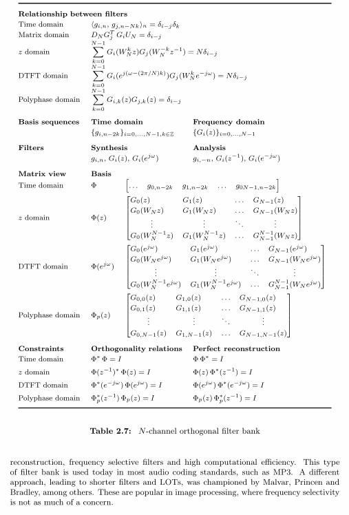
Historical Remarks 89
Relationship between filters
Time domain 〈gi,n, gj,n−Nk〉n = δi−jδkMatrix domain DNG
Tj GiUN = δi−j
z domain
N−1∑
k=0
Gi(WkNz)Gj(W
−kN z−1) = Nδi−j
DTFT domain
N−1∑
k=0
Gi(ej(ω−(2π/N)k))Gj(W
kN e
−jω) = Nδi−j
Polyphase domain
N−1∑
k=0
Gi,k(z)Gj,k(z) = δi−j
Basis sequences Time domain Frequency domain
gi,n−2ki=0,...,N−1,k∈Z Gi(z)i=0,...,N−1
Filters Synthesis Analysis
gi,n, Gi(z), Gi(ejω) gi,−n, Gi(z
−1), Gi(e−jω)
Matrix view Basis
Time domain Φ[. . . g0,n−2k g1,n−2k . . . g0N−1,n−2k
]
z domain Φ(z)
G0(z) G1(z) . . . GN−1(z)
G0(WNz) G1(WNz) . . . GN−1(WNz)...
.... . .
...
G0(WN−1N z) G1(W
N−1N z) . . . GN−1
N−1(WNz)
DTFT domain Φ(ejω)
G0(ejω) G1(ejω) . . . GN−1(ejω)
G0(WNejω) G1(WN e
jω) . . . GN−1(WN ejω)
......
. . ....
G0(WN−1N ejω) G1(W
N−1N ejω) . . . GN−1
N−1(WN ejω)
Polyphase domain Φp(z)
G0,0(z) G1,0(z) . . . GN−1,0(z)
G0,1(z) G1,1(z) . . . GN−1,1(z)...
.... . .
...
G0,N−1(z) G1,N−1(z) . . . GN−1,N−1(z)
Constraints Orthogonality relations Perfect reconstruction
Time domain Φ∗ Φ = I ΦΦ∗ = I
z domain Φ(z−1)∗ Φ(z) = I Φ(z) Φ∗(z−1) = I
DTFT domain Φ∗(e−jω)Φ(ejω) = I Φ(ejω)Φ∗(e−jω) = I
Polyphase domain Φ∗p(z
−1)Φp(z) = I Φp(z)Φ∗p(z
−1) = I
Table 2.7: N-channel orthogonal filter bank
reconstruction, frequency selective filters and high computational efficiency. This typeof filter bank is used today in most audio coding standards, such as MP3. A differentapproach, leading to shorter filters and LOTs, was championed by Malvar, Princen andBradley, among others. These are popular in image processing, where frequency selectivityis not as much of a concern.
90 Chapter 2. Local Fourier Bases on Sequences
Wi-Fi Frequency division multiplexing has been a popular com-
munications method since the 1960’s, and its digital version led to
complex exponential-modulated transmultiplexers with FFTs, as
proposed by Bellanger and co-workers. That perfect transmul-
tiplexing is possible was pointed out by Vetterli. Multicarrier
frequency signaling, which relies on efficient complex exponential-modulated transmulti-
plexers is one of the main communications methods, with orthogonal frequency division
multiplexing (OFDM) being at the heart of many standards (for example, Wi-Fi, 802.11).
Further Reading
Books and Textbooks For a general treatment of N-channel filter banks, see the booksby Vaidyanathan [98], Vetterli and Kovacevic [106], Strang and Nguyen [87], among oth-ers. For modulated filter banks, see [98] as well as Malvar’s book [61], the latter with aparticular emphasis on LOTs. For a good basic discussion of periodograms, see Porat’sbook on signal processing [68], while a more advanced treatment of spectral estimationcan be found in Porat’s book on statistical signal processing [67], and Stoica and Moses’book on spectral estimation [86].
Design of N -Channel Filter Banks General N-channel filter
bank designs were investigated in [96,97]. The freedom in design
offered by more channels shows in examples such as linear-phase,
orthogonal FIR solutions, not possible in the two-channel case [84,108].
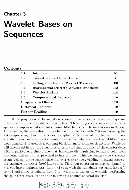
Chapter 3
Wavelet Bases on
Sequences
Contents
3.1 Introduction 93
3.2 Tree-Structured Filter Banks 99
3.3 Orthogonal Discrete Wavelet Transform 106
3.4 Biorthogonal Discrete Wavelet Transform 112
3.5 Wavelet Packets 114
3.6 Computational Aspects 116
Chapter at a Glance 118
Historical Remarks 119
Further Reading 119
If the projection of the signal onto two subspaces is advantageous, projectingonto more subspaces might be even better. These projections onto multiple sub-spaces are implemented via multichannel filter banks, which come in various flavors:For example, there are direct multichannel filter banks, with N filters covering theentire spectrum, their outputs downsampled by N , covered in Chapter 2. Thereare also tree-structured multichannel filter banks, where a two-channel filter bankfrom Chapter 1 is used as a building block for more complex structures. While wewill discuss arbitrary tree structures later in this chapter, most of the chapter dealswith a particularly simple one that has some distinguishing features, both frommathematical as well as practical points of view. This elementary tree structurerecursively splits the coarse space into ever coarser ones, yielding, in signal process-ing parlance, an octave-band filter bank. The input spectrum (subspace) from 0 toπ is cut into a highpass part from π/2 to π, with the remainder cut again into π/4to π/2 and a new remainder from 0 to π/4, and so on. As an example, performingthe split three times leads to the following 4-channel spectral division:
[0,π
8
),[π8,π
4
),[π4,π
2
),[π2, π),
91
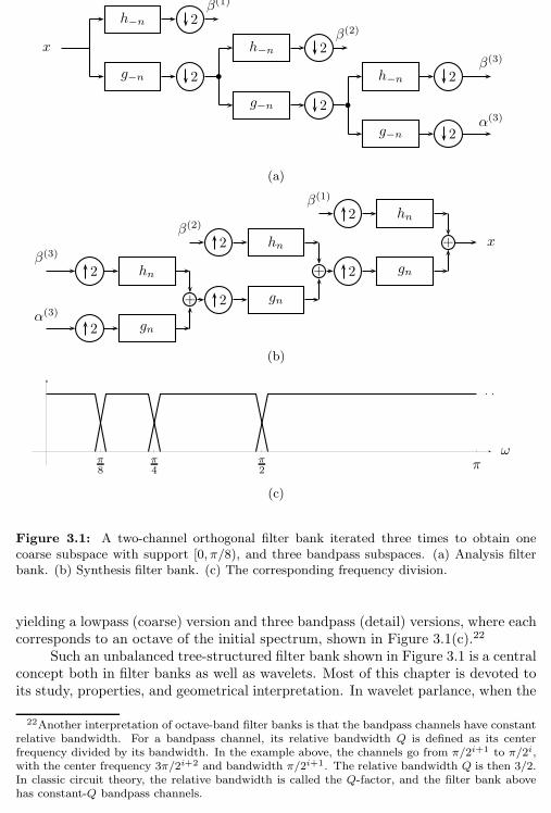
92 Chapter 3. Wavelet Bases on Sequences
x
h−n 2
g−n 2
β(1)
h−n 2
g−n 2
β(2)
h−n 2
g−n 2
β(3)
α(3)
(a)
β(3)
α(3)
2 hn
2 gn
+
β(2)
2 hn
2 gn
+
β(1)
2 hn
2 gn
+ x
(b)
ωπ
8π
4π
2 π
(c)
Figure 3.1: A two-channel orthogonal filter bank iterated three times to obtain onecoarse subspace with support [0, π/8), and three bandpass subspaces. (a) Analysis filterbank. (b) Synthesis filter bank. (c) The corresponding frequency division.
yielding a lowpass (coarse) version and three bandpass (detail) versions, where eachcorresponds to an octave of the initial spectrum, shown in Figure 3.1(c).22
Such an unbalanced tree-structured filter bank shown in Figure 3.1 is a centralconcept both in filter banks as well as wavelets. Most of this chapter is devoted toits study, properties, and geometrical interpretation. In wavelet parlance, when the
22Another interpretation of octave-band filter banks is that the bandpass channels have constantrelative bandwidth. For a bandpass channel, its relative bandwidth Q is defined as its centerfrequency divided by its bandwidth. In the example above, the channels go from π/2i+1 to π/2i,with the center frequency 3π/2i+2 and bandwidth π/2i+1. The relative bandwidth Q is then 3/2.In classic circuit theory, the relative bandwidth is called the Q-factor, and the filter bank abovehas constant-Q bandpass channels.
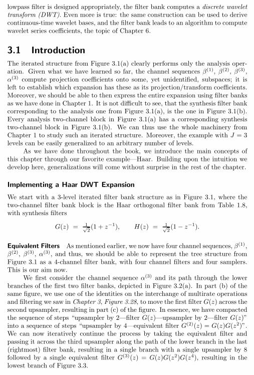
3.1. Introduction 93
lowpass filter is designed appropriately, the filter bank computes a discrete wavelettransform (DWT). Even more is true: the same construction can be used to derivecontinuous-time wavelet bases, and the filter bank leads to an algorithm to computewavelet series coefficients, the topic of Chapter 6.
3.1 Introduction
The iterated structure from Figure 3.1(a) clearly performs only the analysis oper-ation. Given what we have learned so far, the channel sequences β(1), β(2), β(3),α(3) compute projection coefficients onto some, yet unidentified, subspaces; it isleft to establish which expansion has these as its projection/transform coefficients.Moreover, we should be able to then express the entire expansion using filter banksas we have done in Chapter 1. It is not difficult to see, that the synthesis filter bankcorresponding to the analysis one from Figure 3.1(a), is the one in Figure 3.1(b).Every analysis two-channel block in Figure 3.1(a) has a corresponding synthesistwo-channel block in Figure 3.1(b). We can thus use the whole machinery fromChapter 1 to study such an iterated structure. Moreover, the example with J = 3levels can be easily generalized to an arbitrary number of levels.
As we have done throughout the book, we introduce the main concepts ofthis chapter through our favorite example—Haar. Building upon the intuition wedevelop here, generalizations will come without surprise in the rest of the chapter.
Implementing a Haar DWT Expansion
We start with a 3-level iterated filter bank structure as in Figure 3.1, where thetwo-channel filter bank block is the Haar orthogonal filter bank from Table 1.8,with synthesis filters
G(z) = 1√2(1 + z−1), H(z) = 1√
2(1− z−1).
Equivalent Filters As mentioned earlier, we now have four channel sequences, β(1),β(2), β(3), α(3), and thus, we should be able to represent the tree structure fromFigure 3.1 as a 4-channel filter bank, with four channel filters and four samplers.This is our aim now.
We first consider the channel sequence α(3) and its path through the lowerbranches of the first two filter banks, depicted in Figure 3.2(a). In part (b) of thesame figure, we use one of the identities on the interchange of multirate operationsand filtering we saw in Chapter 3, Figure 3.28, to move the first filter G(z) across thesecond upsampler, resulting in part (c) of the figure. In essence, we have compactedthe sequence of steps “upsampler by 2—filter G(z)—upsampler by 2—filter G(z)”into a sequence of steps “upsampler by 4—equivalent filter G(2)(z) = G(z)G(z2)”.We can now iteratively continue the process by taking the equivalent filter andpassing it across the third upsampler along the path of the lower branch in the last(rightmost) filter bank, resulting in a single branch with a single upsampler by 8followed by a single equivalent filter G(3)(z) = G(z)G(z2)G(z4), resulting in thelowest branch of Figure 3.3.
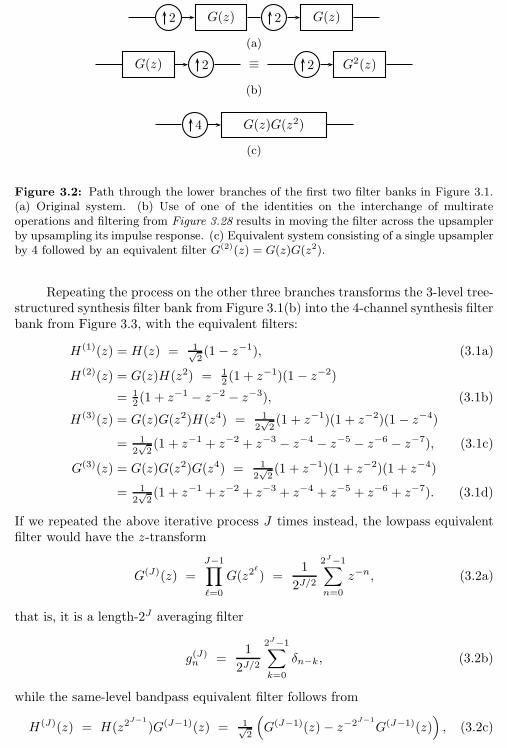
94 Chapter 3. Wavelet Bases on Sequences
2 G(z) 2 G(z)
(a)
G(z) 2 ≡ 2 G2(z)
(b)
4 G(z)G(z2)
(c)
Figure 3.2: Path through the lower branches of the first two filter banks in Figure 3.1.(a) Original system. (b) Use of one of the identities on the interchange of multirateoperations and filtering from Figure 3.28 results in moving the filter across the upsamplerby upsampling its impulse response. (c) Equivalent system consisting of a single upsamplerby 4 followed by an equivalent filter G(2)(z) = G(z)G(z2).
Repeating the process on the other three branches transforms the 3-level tree-structured synthesis filter bank from Figure 3.1(b) into the 4-channel synthesis filterbank from Figure 3.3, with the equivalent filters:
H(1)(z) = H(z) = 1√2(1− z−1), (3.1a)
H(2)(z) = G(z)H(z2) = 12 (1 + z−1)(1 − z−2)
= 12 (1 + z−1 − z−2 − z−3), (3.1b)
H(3)(z) = G(z)G(z2)H(z4) = 12√2(1 + z−1)(1 + z−2)(1 − z−4)
= 12√2(1 + z−1 + z−2 + z−3 − z−4 − z−5 − z−6 − z−7), (3.1c)
G(3)(z) = G(z)G(z2)G(z4) = 12√2(1 + z−1)(1 + z−2)(1 + z−4)
= 12√2(1 + z−1 + z−2 + z−3 + z−4 + z−5 + z−6 + z−7). (3.1d)
If we repeated the above iterative process J times instead, the lowpass equivalentfilter would have the z-transform
G(J)(z) =J−1∏
ℓ=0
G(z2ℓ
) =1
2J/2
2J−1∑
n=0
z−n, (3.2a)
that is, it is a length-2J averaging filter
g(J)n
=1
2J/2
2J−1∑
k=0
δn−k, (3.2b)
while the same-level bandpass equivalent filter follows from
H(J)(z) = H(z2J−1
)G(J−1)(z) = 1√2
(G(J−1)(z)− z−2J−1
G(J−1)(z)), (3.2c)
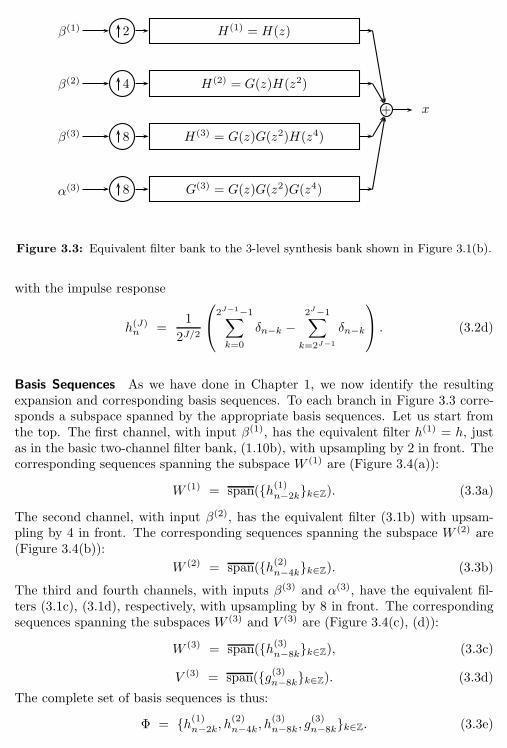
3.1. Introduction 95
β(1)
β(2)
β(3)
α(3)
2 H(1) = H(z)
4 H(2) = G(z)H(z2)
8 H(3) = G(z)G(z2)H(z4)
8 G(3) = G(z)G(z2)G(z4)
+ x
Figure 3.3: Equivalent filter bank to the 3-level synthesis bank shown in Figure 3.1(b).
with the impulse response
h(J)n
=1
2J/2
2J−1−1∑
k=0
δn−k −2J−1∑
k=2J−1
δn−k
. (3.2d)
Basis Sequences As we have done in Chapter 1, we now identify the resultingexpansion and corresponding basis sequences. To each branch in Figure 3.3 corre-sponds a subspace spanned by the appropriate basis sequences. Let us start fromthe top. The first channel, with input β(1), has the equivalent filter h(1) = h, justas in the basic two-channel filter bank, (1.10b), with upsampling by 2 in front. Thecorresponding sequences spanning the subspace W (1) are (Figure 3.4(a)):
W (1) = span(h(1)n−2kk∈Z). (3.3a)
The second channel, with input β(2), has the equivalent filter (3.1b) with upsam-pling by 4 in front. The corresponding sequences spanning the subspace W (2) are(Figure 3.4(b)):
W (2) = span(h(2)n−4kk∈Z). (3.3b)
The third and fourth channels, with inputs β(3) and α(3), have the equivalent fil-ters (3.1c), (3.1d), respectively, with upsampling by 8 in front. The correspondingsequences spanning the subspaces W (3) and V (3) are (Figure 3.4(c), (d)):
W (3) = span(h(3)n−8kk∈Z), (3.3c)
V (3) = span(g(3)n−8kk∈Z). (3.3d)
The complete set of basis sequences is thus:
Φ = h(1)n−2k, h
(2)n−4k, h
(3)n−8k, g
(3)n−8kk∈Z. (3.3e)
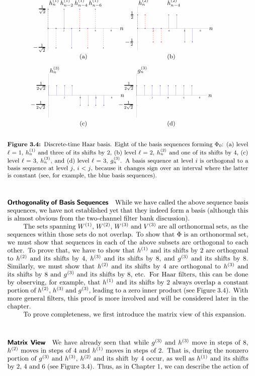
96 Chapter 3. Wavelet Bases on Sequences
2 4 6 8 n
− 1√2
1√2
h(1)n h
(1)n−2 h
(1)n−4 h
(1)n−6
2 4 6 8n
− 12
12
h(2)n h
(2)n−4
(a) (b)
2 4 6 8n
− 1
2√
2
1
2√
2
h(3)n
2 4 6 8n
− 1
2√
2
1
2√
2
g(3)n
(c) (d)
Figure 3.4: Discrete-time Haar basis. Eight of the basis sequences forming Φ0: (a) level
ℓ = 1, h(1)n and three of its shifts by 2, (b) level ℓ = 2, h
(2)n and one of its shifts by 4, (c)
level ℓ = 3, h(3)n , and (d) level ℓ = 3, g
(3)n . A basis sequence at level i is orthogonal to a
basis sequence at level j, i < j, because it changes sign over an interval where the latteris constant (see, for example, the blue basis sequences).
Orthogonality of Basis Sequences While we have called the above sequence basissequences, we have not established yet that they indeed form a basis (although thisis almost obvious from the two-channel filter bank discussion).
The sets spanning W (1), W (2), W (3) and V (3) are all orthonormal sets, as thesequences within those sets do not overlap. To show that Φ is an orthonormal set,we must show that sequences in each of the above subsets are orthogonal to eachother. To prove that, we have to show that h(1) and its shifts by 2 are orthogonalto h(2) and its shifts by 4, h(3) and its shifts by 8, and g(3) and its shifts by 8.Similarly, we must show that h(2) and its shifts by 4 are orthogonal to h(3) andits shifts by 8 and g(3) and its shifts by 8, etc. For Haar filters, this can be doneby observing, for example, that h(1) and its shifts by 2 always overlap a constantportion of h(2), h(3) and g(3), leading to a zero inner product (see Figure 3.4). Withmore general filters, this proof is more involved and will be considered later in thechapter.
To prove completeness, we first introduce the matrix view of this expansion.
Matrix View We have already seen that while g(3) and h(3) move in steps of 8,h(2) moves in steps of 4 and h(1) moves in steps of 2. That is, during the nonzeroportion of g(3) and h(3), h(2) and its shift by 4 occur, as well as h(1) and its shiftsby 2, 4 and 6 (see Figure 3.4). Thus, as in Chapter 1, we can describe the action of
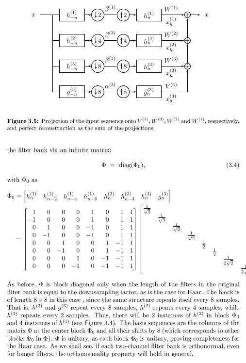
3.1. Introduction 97
x h(1)−n 2
h(2)−n 4
h(3)−n 8
g(3)−n 8
β(1)
β(2)
β(3)
α(3)
2 h(1)n
4 h(2)n
8 h(3)n
8 g(3)n
+
+
+W (1)
W (2)
W (3)
V (4)
x(1)h
x(2)h
x(3)h
x(3)g
x
Figure 3.5: Projection of the input sequence onto V (3),W (3),W (2) andW (1), respectively,and perfect reconstruction as the sum of the projections.
the filter bank via an infinite matrix:
Φ = diag(Φ0), (3.4)
with Φ0 as
Φ0 =[h(1)n h
(1)n−2 h
(1)n−4 h
(1)n−6 h
(2)n h
(2)n−4 h
(3)n g
(3)n
]
=
1 0 0 0 1 0 1 1−1 0 0 0 1 0 1 10 1 0 0 −1 0 1 10 −1 0 0 −1 0 1 10 0 1 0 0 1 −1 10 0 −1 0 0 1 −1 10 0 0 1 0 −1 −1 10 0 0 −1 0 −1 −1 1
1√2
1√2
1√2
1√2
12
12
12√2
12√2
.
As before, Φ is block diagonal only when the length of the filters in the originalfilter bank is equal to the downsampling factor, as is the case for Haar. The block isof length 8× 8 in this case , since the same structure repeats itself every 8 samples.That is, h(3) and g(3) repeat every 8 samples, h(2) repeats every 4 samples, whileh(1) repeats every 2 samples. Thus, there will be 2 instances of h(2) in block Φ0
and 4 instances of h(1) (see Figure 3.4). The basis sequences are the columns of thematrix Φ at the center block Φ0 and all their shifts by 8 (which corresponds to otherblocks Φ0 in Φ). Φ is unitary, as each block Φ0 is unitary, proving completeness forthe Haar case. As we shall see, if each two-channel filter bank is orthonormal, evenfor longer filters, the orthonormality property will hold in general.
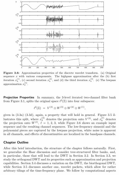
98 Chapter 3. Wavelet Bases on Sequences
−2
0
2x
−0.5
0
0.5x
h(1)
−0.5
0
0.5
xh(2)
−0.2
0
0.2
xh(3)
0 100 200 300 400 500 600 700 800 900 1000
−1
0
1x
g(3)
Figure 3.6: Approximation properties of the discrete wavelet transform. (a) Originalsequence x with various components. The highpass approximation after the (b) first
iteration x(1)h , (c) second iteration x
(2)h , and (d) the third iteration x
(3)h . (e) The lowpass
approximation x(3)g .
Projection Properties In summary, the 3-level iterated two-channel filter bankfrom Figure 3.1, splits the original space ℓ2(Z) into four subspaces:
ℓ2(Z) = V (3) ⊕W (3) ⊕W (2) ⊕W (1),
given in (3.3a)–(3.3d), again, a property that will hold in general. Figure 3.5 il-
lustrates this split, where x(3)g denotes the projection onto V (3), and x
(ℓ)h
denotesthe projection onto W (ℓ), ℓ = 1, 2, 3, while Figure 3.6 shows an example inputsequence and the resulting channel sequences. The low-frequency sinusoid and thepolynomial pieces are captured by the lowpass projection, white noise is apparentin all channels, and effects of discontinuities are localized in the bandpass channels.
Chapter Outline
After this brief introduction, the structure of the chapter follows naturally. First,we generalize the Haar discussion and consider tree-structured filter banks, and,in particular, those that will lead to the DWT in Section 3.2. In Section 3.3, westudy the orthogonal DWT and its properties such as approximation and projectioncapabilities. Section 3.4 discusses a variation on the DWT, the biorthogonal DWT,while Section 3.5 discusses another one, wavelet packets, which allow for ratherarbitrary tilings of the time-frequency plane. We follow by computational aspects
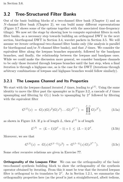
3.2. Tree-Structured Filter Banks 99
in Section 3.6.
3.2 Tree-Structured Filter Banks
Out of the basic building blocks of a two-channel filter bank (Chapter 1) and anN -channel filter bank (Chapter 2), we can build many different representations(Figure 3.7 shows some of the options together with the associated time-frequencytilings). We now set the stage by showing how to compute equivalent filters in suchfilter banks, as a necessary step towards building an orthogonal DWT in the nextsection, biorthogonal DWT in Section 3.4, wavelet packets in Section 3.5. We willassume we iterate orthogonal two-channel filter banks only (the analysis is parallelfor biorthogonal and/or N -channel filter banks), and that J times. We consider theequivalent filter along the lowpass branches separately, followed by the bandpassbranches, and finally, the relationship between the lowpass and bandpass ones.While we could make the discussion more general, we consider bandpass channelsto be only those iterated through lowpass branches until the last step, when a finaliteration is through a highpass one, as is the case for the DWT (iterations througharbitrary combinations of lowpass and highpass branches would follow similarly).
3.2.1 The Lowpass Channel and Its Properties
We start with the lowpass channel iterated J times, leading to g(J). Using the sameidentity to move the filter past the upsampler as in Figure 3.2, a cascade of J timesupsampling and filtering by G(z) leads to upsampling by 2J followed by filteringwith the equivalent filter
G(J)(z) = G(z)G(z2)G(z4) . . . G(z2J−1
) =
J−1∏
ℓ=0
G(z2ℓ
), (3.5a)
as shown in Figure 3.8. If g is of length L, then g(J) is of length
L(J) = (L− 1)(2J − 1) + 1 ≤ (L− 1) 2J . (3.5b)
Moreover, we see that
G(J)(z) = G(z)G(J−1)(z2) = G(J−1)(z)G(z2J−1
). (3.5c)
Some other recursive relations are given in Exercise ??.
Orthogonality of the Lowpass Filter We can use the orthogonality of the basictwo-channel synthesis building block to show the orthogonality of the synthesisoperator obtained by iterating. From this it must be true that the iterated lowpassfilter is orthogonal to its translates by 2J . As in Section 1.2.1, we summarize theorthogonality properties here (as the proof is just a straightforward, albeit tedious,
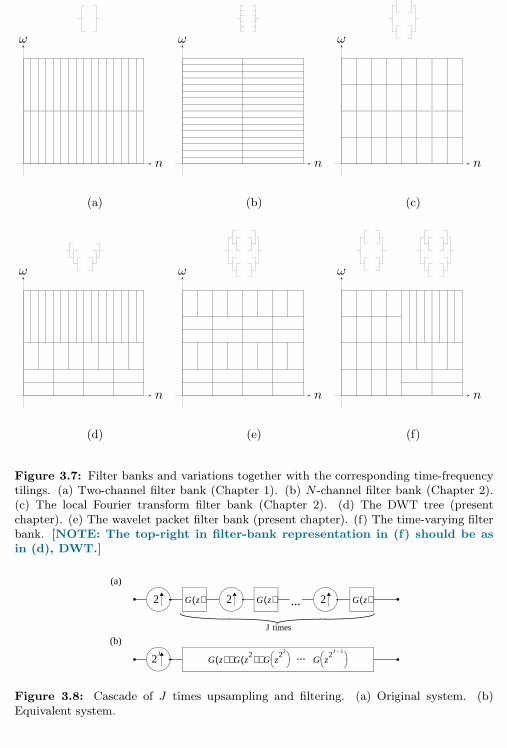
100 Chapter 3. Wavelet Bases on Sequences
n
ω
n
ω
n
ω
(a) (b) (c)
n
ω
n
ω
n
ω
(d) (e) (f)
Figure 3.7: Filter banks and variations together with the corresponding time-frequencytilings. (a) Two-channel filter bank (Chapter 1). (b) N-channel filter bank (Chapter 2).(c) The local Fourier transform filter bank (Chapter 2). (d) The DWT tree (presentchapter). (e) The wavelet packet filter bank (present chapter). (f) The time-varying filterbank. [NOTE: The top-right in filter-bank representation in (f) should be asin (d), DWT.]
2
(a)
(b)
...
J times
2 2 2G z( ) G z( ) G z( )
G z( ) G z2( ) G z
22
⋅ ⋅ G z
2J 1–
...J
Figure 3.8: Cascade of J times upsampling and filtering. (a) Original system. (b)Equivalent system.
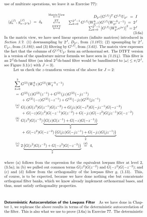
3.2. Tree-Structured Filter Banks 101
use of multirate operations, we leave it as Exercise ??):
〈g(J)n, g
(J)
n−2Jk〉 = δk
MatrixView←→ D2J (G(J))T G(J)U2J = I
ZT←→ ∑2J−1k=0 G(J)(W k
2J z)G(J)(W−k
2Jz−1) = 2J
DTFT←→ ∑2J−1k=0
∣∣G(J)(W k
2J ejω)∣∣2 = 2J
(3.6a)In the matrix view, we have used linear operators (infinite matrices) introduced inSection 3.7: (1) downsampling by 2J , D2J , from (3.187); (2) upsampling by 2J ,U2J , from (3.192); and (3) filtering by G(J), from (3.62). The matrix view expressesthe fact that the columns of G(J)U2J form an orthonormal set. The DTFT versionis a version of the quadrature mirror formula we have seen in (3.214). This filter isan 2Jth-band filter (an ideal 2Jth-band filter would be bandlimited to |ω| ≤ π/2J ,see Figure 3.1(c) with J = 3).
Let us check the z-transform version of the above for J = 2:
3∑
k=0
G(2)(W k
4 z)G(2)(W−k
4 z−1)
= G(2)(z)G(2)(z−1) +G(2)(jz)G(2)(−jz−1)
+ G(2)(−z)G(2)(−z−1) +G(2)(−jz)G(2)(jz−1)
(a)= G(z)G(z2)G(z−1)G(z−2) +G(jz)G(−z2)G(−jz−1)G(−z−2)
+ G(−z)G(z2)G(−z−1)G(z−2) +G(−jz)G(−z2)G(jz−1)G(−z−2)
(b)= G(z2)G(z−2)
(G(z)G(z−1) +G(−z)G(−z−1)
)︸ ︷︷ ︸
2
+ G(−z2)G(−z−2)(G(jz)G(−jz−1) +G(−jz)G(jz−1)
)︸ ︷︷ ︸
2
(c)= 2
(G(z2)G(z−2) +G(−z2)G(−z−2)
)︸ ︷︷ ︸
2
(d)= 4,
where (a) follows from the expression for the equivalent lowpass filter at level 2,(3.5a); in (b) we pulled out common terms G(z2)G(z−2) and G(−z2)G(−z−2); and(c) and (d) follow from the orthogonality of the lowpass filter g, (1.13). This,of course, is to be expected, because we have done nothing else but concatenateorthogonal filter banks, which we know already implement orthonormal bases, andthus, must satisfy orthogonality properties.
Deterministic Autocorrelation of the Lowpass Filter As we have done in Chap-ter 1, we rephrase the above results in terms of the deterministic autocorrelation ofthe filter. This is also what we use to prove (3.6a) in Exercise ??. The deterministic
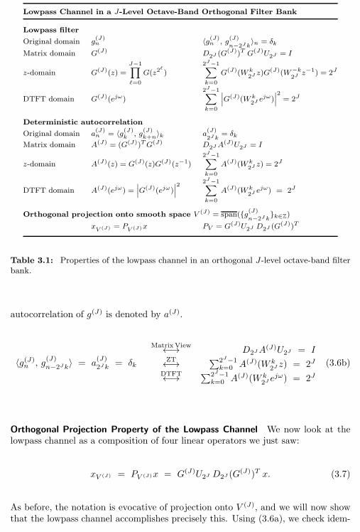
102 Chapter 3. Wavelet Bases on Sequences
Lowpass Channel in a J-Level Octave-Band Orthogonal Filter Bank
Lowpass filter
Original domain g(J)n 〈g(J)n , g
(J)
n−2Jk〉n = δk
Matrix domain G(J) D2J (G(J))T G(J)U2J = I
z-domain G(J)(z) =
J−1∏
ℓ=0
G(z2ℓ
)
2J−1∑
k=0
G(J)(W k2Jz)G(J)(W−k
2Jz−1) = 2J
DTFT domain G(J)(ejω)
2J−1∑
k=0
∣∣∣G(J)(W k2Jejω)
∣∣∣2= 2J
Deterministic autocorrelation
Original domain a(J)n = 〈g(J)k , g
(J)k+n〉k a
(J)
2Jk= δk
Matrix domain A(J) = (G(J))TG(J) D2JA(J)U2J = I
z-domain A(J)(z) = G(J)(z)G(J)(z−1)
2J−1∑
k=0
A(J)(W k2Jz) = 2J
DTFT domain A(J)(ejω) =∣∣∣G(J)(ejω)
∣∣∣2
2J−1∑
k=0
A(J)(W k2Jejω) = 2J
Orthogonal projection onto smooth space V (J) = span(g(J)n−2Jk
k∈Z)
xV (J) = PV (J)x PV = G(J)U2J D2J (G(J))T
Table 3.1: Properties of the lowpass channel in an orthogonal J-level octave-band filterbank.
autocorrelation of g(J) is denoted by a(J).
〈g(J)n, g
(J)
n−2Jk〉 = a(J)
2Jk = δk
MatrixView←→ D2JA(J)U2J = I
ZT←→ ∑2J−1k=0 A(J)(W k
2J z) = 2J
DTFT←→ ∑2J−1k=0 A(J)(W k
2J ejω) = 2J
(3.6b)
Orthogonal Projection Property of the Lowpass Channel We now look at thelowpass channel as a composition of four linear operators we just saw:
xV
(J) = PV
(J)x = G(J)U2J D2J (G(J))T x. (3.7)
As before, the notation is evocative of projection onto V (J), and we will now showthat the lowpass channel accomplishes precisely this. Using (3.6a), we check idem-
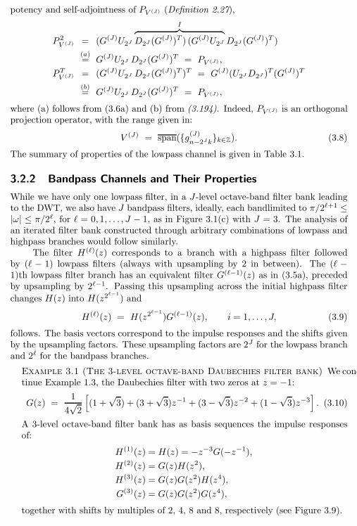
3.2. Tree-Structured Filter Banks 103
potency and self-adjointness of PV
(J) (Definition 2.27),
P 2V
(J) = (G(J)U2J
I︷ ︸︸ ︷D2J (G
(J))T ) (G(J)U2J D2J (G(J))T )
(a)= G(J)U2J D2J (G
(J))T = PV
(J) ,
PTV
(J) = (G(J)U2J D2J (G(J))T )T = G(J)(U2JD2J )
T (G(J))T
(b)= G(J)U2J D2J (G
(J))T = PV
(J) ,
where (a) follows from (3.6a) and (b) from (3.194). Indeed, PV
(J) is an orthogonalprojection operator, with the range given in:
V (J) = span(g(J)n−2Jk
k∈Z). (3.8)
The summary of properties of the lowpass channel is given in Table 3.1.
3.2.2 Bandpass Channels and Their Properties
While we have only one lowpass filter, in a J-level octave-band filter bank leadingto the DWT, we also have J bandpass filters, ideally, each bandlimited to π/2ℓ+1 ≤|ω| ≤ π/2ℓ, for ℓ = 0, 1, . . . , J − 1, as in Figure 3.1(c) with J = 3. The analysis ofan iterated filter bank constructed through arbitrary combinations of lowpass andhighpass branches would follow similarly.
The filter H(ℓ)(z) corresponds to a branch with a highpass filter followedby (ℓ − 1) lowpass filters (always with upsampling by 2 in between). The (ℓ −1)th lowpass filter branch has an equivalent filter G(ℓ−1)(z) as in (3.5a), precededby upsampling by 2ℓ−1. Passing this upsampling across the initial highpass filter
changes H(z) into H(z2ℓ−1
) and
H(ℓ)(z) = H(z2ℓ−1
)G(ℓ−1)(z), i = 1, . . . , J, (3.9)
follows. The basis vectors correspond to the impulse responses and the shifts givenby the upsampling factors. These upsampling factors are 2J for the lowpass branchand 2ℓ for the bandpass branches.
Example 3.1 (The 3-level octave-band Daubechies filter bank) We con-tinue Example 1.3, the Daubechies filter with two zeros at z = −1:
G(z) =1
4√2
[(1 +
√3) + (3 +
√3)z−1 + (3 −
√3)z−2 + (1−
√3)z−3
]. (3.10)
A 3-level octave-band filter bank has as basis sequences the impulse responsesof:
H(1)(z) = H(z) = −z−3G(−z−1),
H(2)(z) = G(z)H(z2),
H(3)(z) = G(z)G(z2)H(z4),
G(3)(z) = G(z)G(z2)G(z4),
together with shifts by multiples of 2, 4, 8 and 8, respectively (see Figure 3.9).
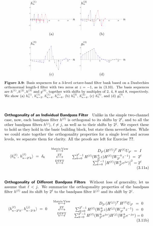
104 Chapter 3. Wavelet Bases on Sequences
5 10 15 20
-2
2
4
n
h(1)n
5 10 15 20
-2
2
4
n
h(2)n
(a) (b)
5 10 15 20
-2
2
4
n
h(3)n
5 10 15 20
-2
2
4
n
g(3)n
(c) (d)
Figure 3.9: Basis sequences for a 3-level octave-band filter bank based on a Daubechiesorthonormal length-4 filter with two zeros at z = −1, as in (3.10). The basis sequencesare h(1), h(2), h(3) and g(3), together with shifts by multiples of 2, 4, 8 and 8, respectively.We show (a) h
(1)n , h
(1)n−2, h
(1)n−4, h
(1)n−6, (b) h
(2)n , h
(2)n−4, (c) h
(3)n , and (d) g
(3)n .
Orthogonality of an Individual Bandpass Filter Unlike in the simple two-channelcase, now, each bandpass filter h(ℓ) is orthogonal to its shifts by 2ℓ, and to all theother bandpass filters h(j), ℓ 6= j, as well as to their shifts by 2j. We expect theseto hold as they hold in the basic building block, but state them nevertheless. Whilewe could state together the orthogonality properties for a single level and acrosslevels, we separate them for clarity. All the proofs are left for Exercise ??.
〈h(ℓ)n, h
(ℓ)
n−2ℓk〉 = δk
MatrixView←→ D2ℓ(H(ℓ))T H(ℓ)U2ℓ = I
ZT←→ ∑2ℓ−1k=0 H(ℓ)(W k
2ℓz)H(ℓ)(W−k
2ℓz−1) = 2ℓ
DTFT←→ ∑2ℓ−1k=0
∣∣H(ℓ)(W k
2ℓejω)∣∣2 = 2ℓ
(3.11a)
Orthogonality of Different Bandpass Filters Without loss of generality, let usassume that ℓ < j. We summarize the orthogonality properties of the bandpassfilter h(ℓ) and its shift by 2ℓ to the bandpass filter h(j) and its shift by 2j.
〈h(ℓ)n−2ℓk
, h(j)n−2jk〉 = 0
MatrixView←→ D2j (H(j))T H(ℓ)U2ℓ = 0
ZT←→∑2ℓ−1k=0 H(ℓ)(W k
2ℓz)H(j)(W−k
2ℓz−1) = 0
DTFT←→ ∑2ℓ−1k=0 H(ℓ)(W k
2ℓejω)H(j)(W k
2ℓe−jω) = 0
(3.11b)
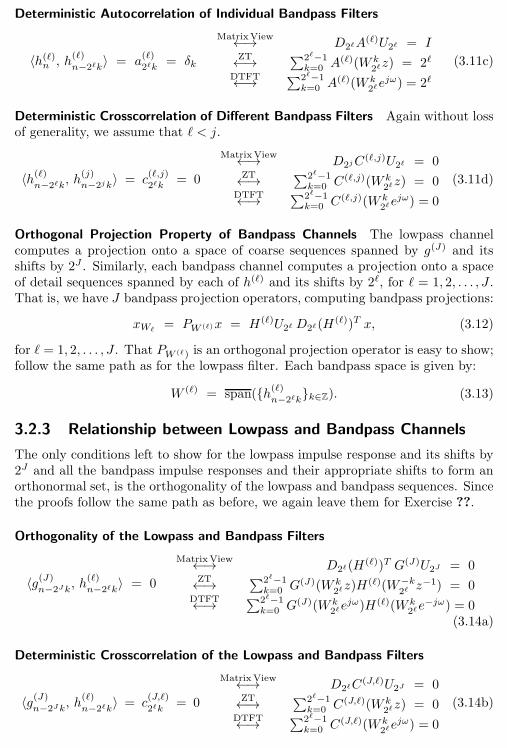
3.2. Tree-Structured Filter Banks 105
Deterministic Autocorrelation of Individual Bandpass Filters
〈h(ℓ)n, h
(ℓ)
n−2ℓk〉 = a
(ℓ)
2ℓk= δk
MatrixView←→ D2ℓA(ℓ)U2ℓ = I
ZT←→ ∑2ℓ−1k=0 A(ℓ)(W k
2ℓz) = 2ℓ
DTFT←→ ∑2ℓ−1k=0 A(ℓ)(W k
2ℓejω) = 2ℓ
(3.11c)
Deterministic Crosscorrelation of Different Bandpass Filters Again without lossof generality, we assume that ℓ < j.
〈h(ℓ)n−2ℓk
, h(j)n−2jk〉 = c
(ℓ,j)
2ℓk= 0
MatrixView←→ D2jC(ℓ,j)U2ℓ = 0
ZT←→ ∑2ℓ−1k=0 C(ℓ,j)(W k
2ℓz) = 0DTFT←→ ∑2ℓ−1
k=0 C(ℓ,j)(W k
2ℓejω) = 0
(3.11d)
Orthogonal Projection Property of Bandpass Channels The lowpass channelcomputes a projection onto a space of coarse sequences spanned by g(J) and itsshifts by 2J . Similarly, each bandpass channel computes a projection onto a spaceof detail sequences spanned by each of h(ℓ) and its shifts by 2ℓ, for ℓ = 1, 2, . . . , J .That is, we have J bandpass projection operators, computing bandpass projections:
xWℓ= P
W(ℓ)x = H(ℓ)U2ℓ D2ℓ(H
(ℓ))T x, (3.12)
for ℓ = 1, 2, . . . , J . That PW
(ℓ) is an orthogonal projection operator is easy to show;follow the same path as for the lowpass filter. Each bandpass space is given by:
W (ℓ) = span(h(ℓ)n−2ℓk
k∈Z). (3.13)
3.2.3 Relationship between Lowpass and Bandpass Channels
The only conditions left to show for the lowpass impulse response and its shifts by2J and all the bandpass impulse responses and their appropriate shifts to form anorthonormal set, is the orthogonality of the lowpass and bandpass sequences. Sincethe proofs follow the same path as before, we again leave them for Exercise ??.
Orthogonality of the Lowpass and Bandpass Filters
〈g(J)n−2Jk
, h(ℓ)
n−2ℓk〉 = 0
MatrixView←→ D2ℓ(H(ℓ))T G(J)U2J = 0
ZT←→ ∑2ℓ−1k=0 G(J)(W k
2ℓz)H(ℓ)(W−k
2ℓz−1) = 0
DTFT←→ ∑2ℓ−1k=0 G(J)(W k
2ℓejω)H(ℓ)(W k
2ℓe−jω) = 0
(3.14a)
Deterministic Crosscorrelation of the Lowpass and Bandpass Filters
〈g(J)n−2Jk, h
(ℓ)
n−2ℓk〉 = c
(J,ℓ)
2ℓk= 0
MatrixView←→ D2ℓC(J,ℓ)U2J = 0
ZT←→ ∑2ℓ−1k=0 C(J,ℓ)(W k
2ℓz) = 0DTFT←→ ∑2ℓ−1
k=0 C(J,ℓ)(W k
2ℓejω) = 0
(3.14b)
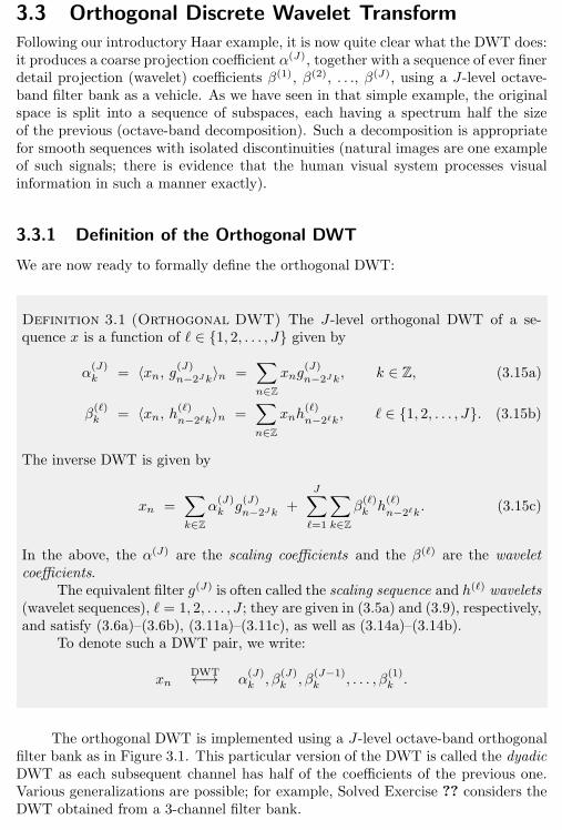
106 Chapter 3. Wavelet Bases on Sequences
3.3 Orthogonal Discrete Wavelet Transform
Following our introductory Haar example, it is now quite clear what the DWT does:it produces a coarse projection coefficient α(J), together with a sequence of ever finerdetail projection (wavelet) coefficients β(1), β(2), . . ., β(J), using a J-level octave-band filter bank as a vehicle. As we have seen in that simple example, the originalspace is split into a sequence of subspaces, each having a spectrum half the sizeof the previous (octave-band decomposition). Such a decomposition is appropriatefor smooth sequences with isolated discontinuities (natural images are one exampleof such signals; there is evidence that the human visual system processes visualinformation in such a manner exactly).
3.3.1 Definition of the Orthogonal DWT
We are now ready to formally define the orthogonal DWT:
Definition 3.1 (Orthogonal DWT) The J-level orthogonal DWT of a se-quence x is a function of ℓ ∈ 1, 2, . . . , J given by
α(J)k
= 〈xn, g(J)n−2Jk〉n =
∑
n∈Z
xng(J)
n−2Jk, k ∈ Z, (3.15a)
β(ℓ)k
= 〈xn, h(ℓ)n−2ℓk
〉n =∑
n∈Z
xnh(ℓ)
n−2ℓk, ℓ ∈ 1, 2, . . . , J. (3.15b)
The inverse DWT is given by
xn =∑
k∈Z
α(J)kg(J)n−2Jk +
J∑
ℓ=1
∑
k∈Z
β(ℓ)kh(ℓ)
n−2ℓk. (3.15c)
In the above, the α(J) are the scaling coefficients and the β(ℓ) are the waveletcoefficients.
The equivalent filter g(J) is often called the scaling sequence and h(ℓ) wavelets(wavelet sequences), ℓ = 1, 2, . . . , J ; they are given in (3.5a) and (3.9), respectively,and satisfy (3.6a)–(3.6b), (3.11a)–(3.11c), as well as (3.14a)–(3.14b).
To denote such a DWT pair, we write:
xnDWT←→ α
(J)k, β
(J)k, β
(J−1)k
, . . . , β(1)k.
The orthogonal DWT is implemented using a J-level octave-band orthogonalfilter bank as in Figure 3.1. This particular version of the DWT is called the dyadicDWT as each subsequent channel has half of the coefficients of the previous one.Various generalizations are possible; for example, Solved Exercise ?? considers theDWT obtained from a 3-channel filter bank.
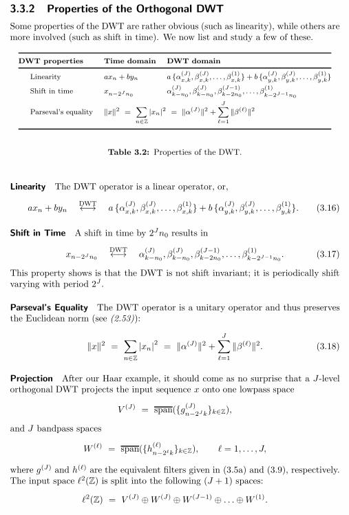
3.3. Orthogonal Discrete Wavelet Transform 107
3.3.2 Properties of the Orthogonal DWT
Some properties of the DWT are rather obvious (such as linearity), while others aremore involved (such as shift in time). We now list and study a few of these.
DWT properties Time domain DWT domain
Linearity axn + byn a α(J)x,k, β
(J)x,k , . . . , β
(1)x,k+ b α(J)
y,k , β(J)y,k , . . . , β
(1)y,k
Shift in time xn−2Jn0α(J)k−n0
, β(J)k−n0
, β(J−1)k−2n0
, . . . , β(1)
k−2J−1n0
Parseval’s equality ‖x‖2 =∑
n∈Z
|xn|2 = ‖α(J)‖2 +J∑
ℓ=1
‖β(ℓ)‖2
Table 3.2: Properties of the DWT.
Linearity The DWT operator is a linear operator, or,
axn + bynDWT←→ a α(J)
x,k, β
(J)x,k, . . . , β
(1)x,k+ b α(J)
y,k, β
(J)y,k, . . . , β
(1)y,k. (3.16)
Shift in Time A shift in time by 2Jn0 results in
xn−2Jn0
DWT←→ α(J)k−n0
, β(J)k−n0
, β(J−1)k−2n0
, . . . , β(1)k−2J−1
n0. (3.17)
This property shows is that the DWT is not shift invariant; it is periodically shiftvarying with period 2J .
Parseval’s Equality The DWT operator is a unitary operator and thus preservesthe Euclidean norm (see (2.53)):
‖x‖2 =∑
n∈Z
|xn|2 = ‖α(J)‖2 +J∑
ℓ=1
‖β(ℓ)‖2. (3.18)
Projection After our Haar example, it should come as no surprise that a J-levelorthogonal DWT projects the input sequence x onto one lowpass space
V (J) = span(g(J)n−2Jk
k∈Z),
and J bandpass spaces
W (ℓ) = span(h(ℓ)n−2ℓk
k∈Z), ℓ = 1, . . . , J,
where g(J) and h(ℓ) are the equivalent filters given in (3.5a) and (3.9), respectively.The input space ℓ2(Z) is split into the following (J + 1) spaces:
ℓ2(Z) = V (J) ⊕W (J) ⊕W (J−1) ⊕ . . .⊕W (1).
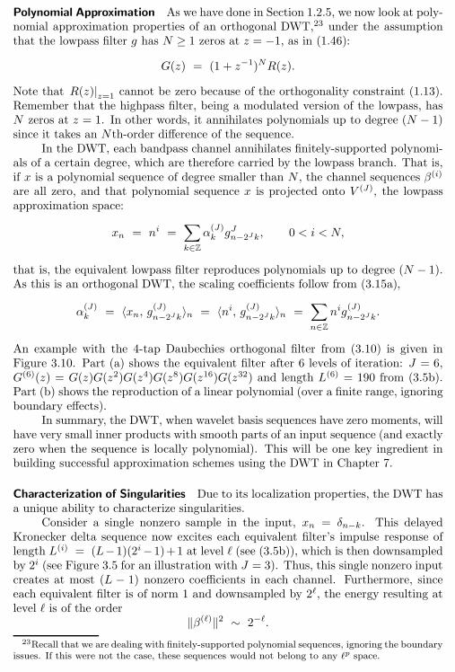
108 Chapter 3. Wavelet Bases on Sequences
Polynomial Approximation As we have done in Section 1.2.5, we now look at poly-nomial approximation properties of an orthogonal DWT,23 under the assumptionthat the lowpass filter g has N ≥ 1 zeros at z = −1, as in (1.46):
G(z) = (1 + z−1)NR(z).
Note that R(z)|z=1 cannot be zero because of the orthogonality constraint (1.13).
Remember that the highpass filter, being a modulated version of the lowpass, hasN zeros at z = 1. In other words, it annihilates polynomials up to degree (N − 1)since it takes an Nth-order difference of the sequence.
In the DWT, each bandpass channel annihilates finitely-supported polynomi-als of a certain degree, which are therefore carried by the lowpass branch. That is,if x is a polynomial sequence of degree smaller than N , the channel sequences β(i)
are all zero, and that polynomial sequence x is projected onto V (J), the lowpassapproximation space:
xn = ni =∑
k∈Z
α(J)kgJn−2Jk, 0 < i < N,
that is, the equivalent lowpass filter reproduces polynomials up to degree (N − 1).As this is an orthogonal DWT, the scaling coefficients follow from (3.15a),
α(J)k
= 〈xn, g(J)n−2Jk
〉n = 〈ni, g(J)n−2Jk
〉n =∑
n∈Z
nig(J)
n−2Jk.
An example with the 4-tap Daubechies orthogonal filter from (3.10) is given inFigure 3.10. Part (a) shows the equivalent filter after 6 levels of iteration: J = 6,G(6)(z) = G(z)G(z2)G(z4)G(z8)G(z16)G(z32) and length L(6) = 190 from (3.5b).Part (b) shows the reproduction of a linear polynomial (over a finite range, ignoringboundary effects).
In summary, the DWT, when wavelet basis sequences have zero moments, willhave very small inner products with smooth parts of an input sequence (and exactlyzero when the sequence is locally polynomial). This will be one key ingredient inbuilding successful approximation schemes using the DWT in Chapter 7.
Characterization of Singularities Due to its localization properties, the DWT hasa unique ability to characterize singularities.
Consider a single nonzero sample in the input, xn = δn−k. This delayedKronecker delta sequence now excites each equivalent filter’s impulse response oflength L(i) = (L−1)(2i−1)+1 at level ℓ (see (3.5b)), which is then downsampledby 2i (see Figure 3.5 for an illustration with J = 3). Thus, this single nonzero inputcreates at most (L − 1) nonzero coefficients in each channel. Furthermore, sinceeach equivalent filter is of norm 1 and downsampled by 2ℓ, the energy resulting atlevel ℓ is of the order
‖β(ℓ)‖2 ∼ 2−ℓ.
23Recall that we are dealing with finitely-supported polynomial sequences, ignoring the boundaryissues. If this were not the case, these sequences would not belong to any ℓp space.
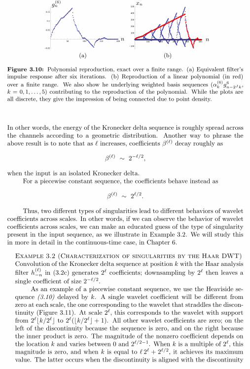
3.3. Orthogonal Discrete Wavelet Transform 109
50 100 150 200
-0.05
0.05
0.1
0.15
n
g(6)n
100 200 300 400 500
-100
100
200
300
400
500
n
xn
(a) (b)
Figure 3.10: Polynomial reproduction, exact over a finite range. (a) Equivalent filter’simpulse response after six iterations. (b) Reproduction of a linear polynomial (in red)
over a finite range. We also show he underlying weighted basis sequences (α(6)k g6n−2Jk,
k = 0, 1, . . . , 5) contributing to the reproduction of the polynomial. While the plots areall discrete, they give the impression of being connected due to point density.
In other words, the energy of the Kronecker delta sequence is roughly spread acrossthe channels according to a geometric distribution. Another way to phrase theabove result is to note that as ℓ increases, coefficients β(ℓ) decay roughly as
β(ℓ) ∼ 2−ℓ/2,
when the input is an isolated Kronecker delta.For a piecewise constant sequence, the coefficients behave instead as
β(ℓ) ∼ 2ℓ/2.
Thus, two different types of singularities lead to different behaviors of waveletcoefficients across scales. In other words, if we can observe the behavior of waveletcoefficients across scales, we can make an educated guess of the type of singularitypresent in the input sequence, as we illustrate in Example 3.2. We will study thisin more in detail in the continuous-time case, in Chapter 6.
Example 3.2 (Characterization of singularities by the Haar DWT)Convolution of the Kronecker delta sequence at position k with the Haar analysis
filter h(ℓ)−n in (3.2c) generates 2ℓ coefficients; downsampling by 2ℓ then leaves a
single coefficient of size 2−ℓ/2.As an example of a piecewise constant sequence, we use the Heaviside se-
quence (3.10) delayed by k. A single wavelet coefficient will be different fromzero at each scale, the one corresponding to the wavelet that straddles the discon-tinuity (Figure 3.11). At scale 2ℓ, this corresponds to the wavelet with supportfrom 2ℓ⌊k/2ℓ⌋ to 2ℓ(⌊k/2ℓ⌋ + 1). All other wavelet coefficients are zero; on theleft of the discontinuity because the sequence is zero, and on the right becausethe inner product is zero. The magnitude of the nonzero coefficient depends onthe location k and varies between 0 and 2ℓ/2−1. When k is a multiple of 2ℓ, thismagnitude is zero, and when k is equal to ℓ 2ℓ + 2ℓ/2, it achieves its maximumvalue. The latter occurs when the discontinuity is aligned with the discontinuity
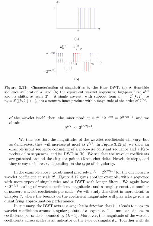
110 Chapter 3. Wavelet Bases on Sequences
n
1
k
xn
(a)
nn1 n2
2−ℓ/2
−2−ℓ/2
h(ℓ)n h
(ℓ)
n−2ℓ
(b)
Figure 3.11: Characterization of singularities by the Haar DWT. (a) A Heavisidesequence at location k, and (b) the equivalent wavelet sequences, highpass filter h(ℓ)
and its shifts, at scale 2ℓ. A single wavelet, with support from n1 = 2ℓ⌊k/2ℓ⌋ ton2 = 2ℓ(⌊k/2ℓ⌋+ 1), has a nonzero inner product with a magnitude of the order of 2ℓ/2.
of the wavelet itself; then, the inner product is 2ℓ−12−ℓ/2 = 2(ℓ/2)−1, and weobtain
β(ℓ) ∼ 2(ℓ/2)−1.
We thus see that the magnitudes of the wavelet coefficients will vary, butas ℓ increases, they will increase at most as 2ℓ/2. In Figure 3.12(a), we show anexample input sequence consisting of a piecewise constant sequence and a Kro-necker delta sequences, and its DWT in (b). We see that the wavelet coefficientsare gathered around the singular points (Kronecker delta, Heaviside step), andthey decay or increase, depending on the type of singularity.
In the example above, we obtained precisely β(ℓ) = 2(ℓ/2)−1 for the one nonzerowavelet coefficient at scale 2ℓ. Figure 3.12 gives another example, with a sequencewith more types of singularities and a DWT with longer filters. We again have∼ 2−ℓ/2 scaling of wavelet coefficient magnitudes and a roughly constant numberof nonzero wavelet coefficients per scale. We will study this effect in more detail inChapter 7, where the bounds on the coefficient magnitudes will play a large role inquantifying approximation performance.
In summary, the DWT acts as a singularity detector, that is, it leads to nonzerowavelet coefficients around singular points of a sequence. The number of nonzerocoefficients per scale is bounded by (L−1). Moreover, the magnitude of the waveletcoefficients across scales is an indicator of the type of singularity. Together with its
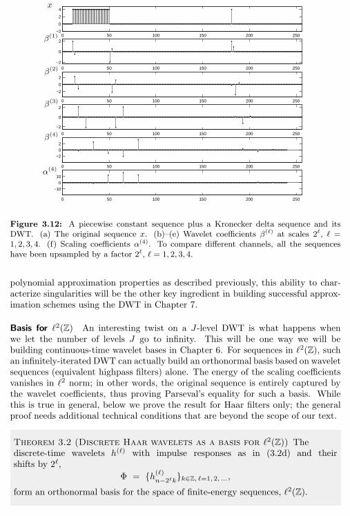
3.3. Orthogonal Discrete Wavelet Transform 111
0 50 100 150 200 250−2
0
2
4
0 50 100 150 200 250−2
0
2
0 50 100 150 200 250
−2
0
2
0 50 100 150 200 250
−2
0
2
0 50 100 150 200 250
−2
0
2
0 50 100 150 200 250
−10
0
10
x
β(1)
β(2)
β(3)
β(4)
α(4)
Figure 3.12: A piecewise constant sequence plus a Kronecker delta sequence and itsDWT. (a) The original sequence x. (b)–(e) Wavelet coefficients β(ℓ) at scales 2ℓ, ℓ =1, 2, 3, 4. (f) Scaling coefficients α(4). To compare different channels, all the sequenceshave been upsampled by a factor 2ℓ, ℓ = 1, 2, 3, 4.
polynomial approximation properties as described previously, this ability to char-acterize singularities will be the other key ingredient in building successful approx-imation schemes using the DWT in Chapter 7.
Basis for ℓ2(Z) An interesting twist on a J-level DWT is what happens whenwe let the number of levels J go to infinity. This will be one way we will bebuilding continuous-time wavelet bases in Chapter 6. For sequences in ℓ2(Z), suchan infinitely-iterated DWT can actually build an orthonormal basis based on waveletsequences (equivalent highpass filters) alone. The energy of the scaling coefficientsvanishes in ℓ2 norm; in other words, the original sequence is entirely captured bythe wavelet coefficients, thus proving Parseval’s equality for such a basis. Whilethis is true in general, below we prove the result for Haar filters only; the generalproof needs additional technical conditions that are beyond the scope of our text.
Theorem 3.2 (Discrete Haar wavelets as a basis for ℓ2(Z)) Thediscrete-time wavelets h(ℓ) with impulse responses as in (3.2d) and theirshifts by 2ℓ,
Φ = h(ℓ)n−2ℓk
k∈Z, ℓ=1, 2, ...,
form an orthonormal basis for the space of finite-energy sequences, ℓ2(Z).
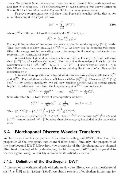
112 Chapter 3. Wavelet Bases on Sequences
Proof. To prove Φ is an orthonormal basis, we must prove it is an orthonormal setand that it is complete. The orthonormality of basis functions was shown earlier inSection 3.1 for Haar filters and in Section 3.2 for the more general ones.
To prove completeness, we will show that Parseval’s equality holds, that is, foran arbitrary input x ∈ ℓ2(Z), we have
‖x‖2 =
∞∑
ℓ=1
‖β(ℓ)‖2, (3.19)
where β(ℓ) are the wavelet coefficients at scales 2ℓ, ℓ = 1, 2, . . .:
β(ℓ)k = 〈xn, h(ℓ)
n−2ℓk〉n.
For any finite number of decomposition levels J , the Parseval’s equality (3.18) holds.Thus, our task is to show limJ→∞ ‖α(J)‖2 = 0. We show this by bounding two quan-tities: the energy lost in truncating x and the energy in the scaling coefficients thatrepresent the truncated sequence.
Without loss of generality, assume x has unit norm. For any ε > 0, we will showthat ‖α(J)‖2 < ε for sufficiently large J . First note that there exists a K such that therestriction of x to −2K , −2K + 1, . . . , 0, 1, . . . , 2K − 1 has energy at least 1 − ε/2;this follows from the convergence of the series defining the ℓ2 norm of x. Denote therestriction by x.
A K-level decomposition of x has at most two nonzero scaling coefficients α(K)−1
and α(K)0 . Each of these scaling coefficients satisfies |α(K)
k | ≤ 1 because ‖α(K)‖2 ≤‖x‖2 = 1 by Bessel’s inequality. We will now consider further levels of decompositionbeyond K. After one more level, the lowpass output α(K+1) has coefficients
α(K+1)0 = 1√
2α(K)0 and α
(K+1)−1 = 1√
2α(K)−1 .
Similarly, after K + j total levels of decomposition we have
α(K+j)k =
1
2j/2α(K)k ≤ 1
2j/2, for k = −1, 0.
Thus, ‖α(K+j)‖2 =(α(K+j)−1
)2
+(α(K+j)0
)2
≤ 2−(j−1).
Let J = K+j where 2−(j−1) < ε/2. Then ‖α(J)‖2 < ε because ‖α(J)‖2 < ε/2 and‖α(J)‖2 cannot exceed ‖α(J)‖2 by more than the energy ε/2 excluded in the truncationof x.
3.4 Biorthogonal Discrete Wavelet Transform
We have seen that the properties of the dyadic orthogonal DWT follow from theproperties of the orthogonal two-channel filter bank. Similarly, the properties ofthe biorthogonal DWT follow from the properties of the biorthogonal two-channelfilter bank. Instead of fully developing the biorthogonal DWT (as it is parallel tothe orthogonal one), we quickly summarize its salient elements.
3.4.1 Definition of the Biorthogonal DWT
If, instead of an orthogonal pair of highpass/lowpass filters, we use a biorthogonal
set h, g, h, g as in (1.64a)–(1.64d), we obtain two sets of equivalent filters, one for
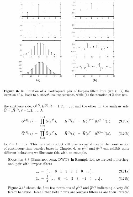
3.4. Biorthogonal Discrete Wavelet Transform 113
−1 0 1 2 3 4 5 60
1
2
3
−1 0 1 2 3 4 5 6−1
−0.5
0
0.5
1
0 2 4 6 8 10 120
5
10
0 2 4 6 8 10 12−1
−0.5
0
0.5
1
0 5 10 15 20 240
20
40
0 5 10 15 20 24−1
−0.5
0
0.5
1
0 10 20 30 40 480
50
100
150
200
0 10 20 30 40 48−1
−0.5
0
0.5
1
(a) (b)
Figure 3.13: Iteration of a biorthogonal pair of lowpass filters from (3.21): (a) theiteration of gn leads to a smooth-looking sequence, while (b) the iteration of g does not.
the synthesis side, G(J), H(ℓ), ℓ = 1, 2, . . . , J , and the other for the analysis side,G(J), H(ℓ), ℓ = 1, 2, . . . , J :
G(J)(z) =
J−1∏
k=0
G(z2k
), H(ℓ)(z) = H(z2ℓ−1
)G(ℓ−1)(z), (3.20a)
G(J)(z) =J−1∏
k=0
G(z2k
), H(ℓ)(z) = H(z2ℓ−1
)G(ℓ−1)(z), (3.20b)
for ℓ = 1, . . . , J . This iterated product will play a crucial role in the constructionof continuous-time wavelet bases in Chapter 6, as g(J) and g(J) can exhibit quitedifferent behaviors; we illustrate this with an example.
Example 3.3 (Biorthogonal DWT) In Example 1.4, we derived a biorthog-onal pair with lowpass filters
gn =[. . . 0 1 3 3 1 0 . . .
], (3.21a)
gn =1
4
[. . . 0 −1 3 3 −1 0 . . .
]. (3.21b)
Figure 3.13 shows the first few iterations of g(J) and g(J) indicating a very dif-ferent behavior. Recall that both filters are lowpass filters as are their iterated
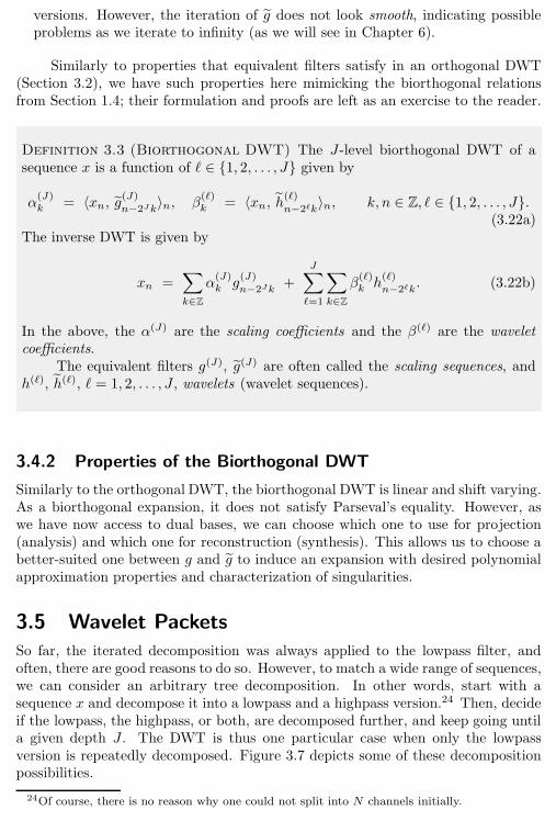
114 Chapter 3. Wavelet Bases on Sequences
versions. However, the iteration of g does not look smooth, indicating possibleproblems as we iterate to infinity (as we will see in Chapter 6).
Similarly to properties that equivalent filters satisfy in an orthogonal DWT(Section 3.2), we have such properties here mimicking the biorthogonal relationsfrom Section 1.4; their formulation and proofs are left as an exercise to the reader.
Definition 3.3 (Biorthogonal DWT) The J-level biorthogonal DWT of asequence x is a function of ℓ ∈ 1, 2, . . . , J given by
α(J)k
= 〈xn, g(J)n−2Jk〉n, β
(ℓ)k
= 〈xn, h(ℓ)n−2ℓk
〉n, k, n ∈ Z, ℓ ∈ 1, 2, . . . , J.(3.22a)
The inverse DWT is given by
xn =∑
k∈Z
α(J)kg(J)
n−2Jk+
J∑
ℓ=1
∑
k∈Z
β(ℓ)kh(ℓ)
n−2ℓk. (3.22b)
In the above, the α(J) are the scaling coefficients and the β(ℓ) are the waveletcoefficients.
The equivalent filters g(J), g(J) are often called the scaling sequences, andh(ℓ), h(ℓ), ℓ = 1, 2, . . . , J , wavelets (wavelet sequences).
3.4.2 Properties of the Biorthogonal DWT
Similarly to the orthogonal DWT, the biorthogonal DWT is linear and shift varying.As a biorthogonal expansion, it does not satisfy Parseval’s equality. However, aswe have now access to dual bases, we can choose which one to use for projection(analysis) and which one for reconstruction (synthesis). This allows us to choose abetter-suited one between g and g to induce an expansion with desired polynomialapproximation properties and characterization of singularities.
3.5 Wavelet Packets
So far, the iterated decomposition was always applied to the lowpass filter, andoften, there are good reasons to do so. However, to match a wide range of sequences,we can consider an arbitrary tree decomposition. In other words, start with asequence x and decompose it into a lowpass and a highpass version.24 Then, decideif the lowpass, the highpass, or both, are decomposed further, and keep going untila given depth J . The DWT is thus one particular case when only the lowpassversion is repeatedly decomposed. Figure 3.7 depicts some of these decompositionpossibilities.
24Of course, there is no reason why one could not split into N channels initially.
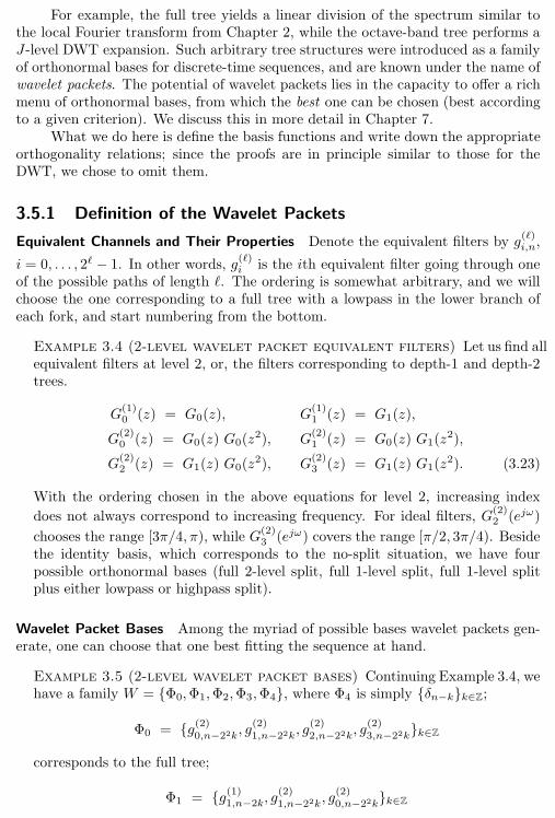
3.5. Wavelet Packets 115
For example, the full tree yields a linear division of the spectrum similar tothe local Fourier transform from Chapter 2, while the octave-band tree performs aJ-level DWT expansion. Such arbitrary tree structures were introduced as a familyof orthonormal bases for discrete-time sequences, and are known under the name ofwavelet packets. The potential of wavelet packets lies in the capacity to offer a richmenu of orthonormal bases, from which the best one can be chosen (best accordingto a given criterion). We discuss this in more detail in Chapter 7.
What we do here is define the basis functions and write down the appropriateorthogonality relations; since the proofs are in principle similar to those for theDWT, we chose to omit them.
3.5.1 Definition of the Wavelet Packets
Equivalent Channels and Their Properties Denote the equivalent filters by g(ℓ)i,n
,
i = 0, . . . , 2ℓ − 1. In other words, g(ℓ)i
is the ith equivalent filter going through oneof the possible paths of length ℓ. The ordering is somewhat arbitrary, and we willchoose the one corresponding to a full tree with a lowpass in the lower branch ofeach fork, and start numbering from the bottom.
Example 3.4 (2-level wavelet packet equivalent filters) Let us find allequivalent filters at level 2, or, the filters corresponding to depth-1 and depth-2trees.
G(1)0 (z) = G0(z), G
(1)1 (z) = G1(z),
G(2)0 (z) = G0(z) G0(z
2), G(2)1 (z) = G0(z) G1(z
2),
G(2)2 (z) = G1(z) G0(z
2), G(2)3 (z) = G1(z) G1(z
2). (3.23)
With the ordering chosen in the above equations for level 2, increasing index
does not always correspond to increasing frequency. For ideal filters, G(2)2 (ejω)
chooses the range [3π/4, π), while G(2)3 (ejω) covers the range [π/2, 3π/4). Beside
the identity basis, which corresponds to the no-split situation, we have fourpossible orthonormal bases (full 2-level split, full 1-level split, full 1-level splitplus either lowpass or highpass split).
Wavelet Packet Bases Among the myriad of possible bases wavelet packets gen-erate, one can choose that one best fitting the sequence at hand.
Example 3.5 (2-level wavelet packet bases) Continuing Example 3.4, wehave a family W = Φ0,Φ1,Φ2,Φ3,Φ4, where Φ4 is simply δn−kk∈Z;
Φ0 = g(2)0,n−22k, g(2)1,n−22k, g
(2)2,n−22k, g
(2)3,n−22kk∈Z
corresponds to the full tree;
Φ1 = g(1)1,n−2k, g(2)1,n−22k, g
(2)0,n−22kk∈Z
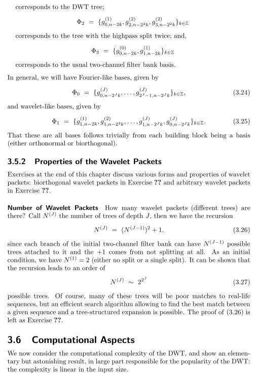
116 Chapter 3. Wavelet Bases on Sequences
corresponds to the DWT tree;
Φ2 = g(1)0,n−2k, g(2)2,n−22k, g
(2)3,n−22kk∈Z
corresponds to the tree with the highpass split twice; and,
Φ3 = g(0)0,n−2k, g(1)1,n−2kk∈Z
corresponds to the usual two-channel filter bank basis.
In general, we will have Fourier-like bases, given by
Φ0 = g(J)0,n−2Jk
, . . . , g(J)
2J−1,n−2Jkk∈Z, (3.24)
and wavelet-like bases, given by
Φ1 = g(1)1,n−2k, g(2)1,n−22k, . . . , g
(J)
1,n−2Jk, g
(J)
0,n−2Jkk∈Z. (3.25)
That these are all bases follows trivially from each building block being a basis(either orthonormal or biorthogonal).
3.5.2 Properties of the Wavelet Packets
Exercises at the end of this chapter discuss various forms and properties of waveletpackets: biorthogonal wavelet packets in Exercise ?? and arbitrary wavelet packetsin Exercise ??.
Number of Wavelet Packets How many wavelet packets (different trees) arethere? Call N (J) the number of trees of depth J , then we have the recursion
N (J) = (N (J−1))2 + 1, (3.26)
since each branch of the initial two-channel filter bank can have N (J−1) possibletrees attached to it and the +1 comes from not splitting at all. As an initialcondition, we have N (1) = 2 (either no split or a single split). It can be shown thatthe recursion leads to an order of
N (J) ∼ 22J
(3.27)
possible trees. Of course, many of these trees will be poor matches to real-lifesequences, but an efficient search algorithm allowing to find the best match betweena given sequence and a tree-structured expansion is possible. The proof of (3.26) isleft as Exercise ??.
3.6 Computational Aspects
We now consider the computational complexity of the DWT, and show an elemen-tary but astonishing result, in large part responsible for the popularity of the DWT:the complexity is linear in the input size.
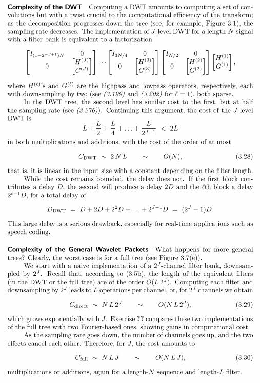
3.6. Computational Aspects 117
Complexity of the DWT Computing a DWT amounts to computing a set of con-volutions but with a twist crucial to the computational efficiency of the transform;as the decomposition progresses down the tree (see, for example, Figure 3.1), thesampling rate decreases. The implementation of J-level DWT for a length-N signalwith a filter bank is equivalent to a factorization
I(1−2−J+1)N 0
0
[H(J)
G(J)
] · · ·
I3N/4 0
0
[H(3)
G(3)
]IN/2 0
0
[H(2)
G(2)
][H(1)
G(1)
],
where H(ℓ)’s and G(ℓ) are the highpass and lowpass operators, respectively, eachwith downsampling by two (see (3.199) and (3.202) for ℓ = 1), both sparse.
In the DWT tree, the second level has similar cost to the first, but at halfthe sampling rate (see (3.276)). Continuing this argument, the cost of the J-levelDWT is
L+L
2+L
4+ . . .+
L
2J−1< 2L
in both multiplications and additions, with the cost of the order of at most
CDWT ∼ 2N L ∼ O(N), (3.28)
that is, it is linear in the input size with a constant depending on the filter length.While the cost remains bounded, the delay does not. If the first block con-
tributes a delay D, the second will produce a delay 2D and the ℓth block a delay2ℓ−1D, for a total delay of
DDWT = D + 2D + 22D + . . .+ 2J−1D = (2J − 1)D.
This large delay is a serious drawback, especially for real-time applications such asspeech coding.
Complexity of the General Wavelet Packets What happens for more generaltrees? Clearly, the worst case is for a full tree (see Figure 3.7(e)).
We start with a naive implementation of a 2J -channel filter bank, downsam-pled by 2J . Recall that, according to (3.5b), the length of the equivalent filters(in the DWT or the full tree) are of the order O(L 2J). Computing each filter anddownsampling by 2J leads to L operations per channel, or, for 2J channels we obtain
Cdirect ∼ N L 2J ∼ O(N L 2J), (3.29)
which grows exponentially with J . Exercise ?? compares these two implementationsof the full tree with two Fourier-based ones, showing gains in computational cost.
As the sampling rate goes down, the number of channels goes up, and the twoeffects cancel each other. Therefore, for J , the cost amounts to
Cfull ∼ N LJ ∼ O(N LJ), (3.30)
multiplications or additions, again for a length-N sequence and length-L filter.
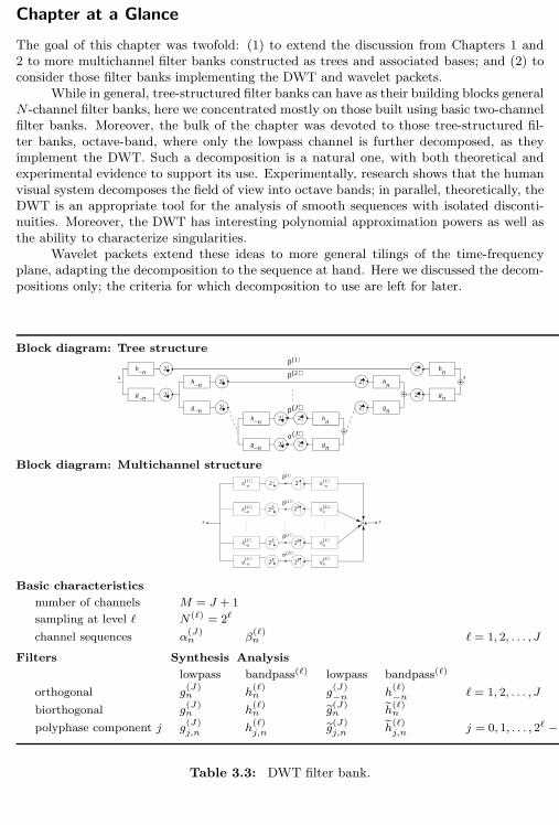
118 Chapter 3. Wavelet Bases on Sequences
Chapter at a Glance
The goal of this chapter was twofold: (1) to extend the discussion from Chapters 1 and2 to more multichannel filter banks constructed as trees and associated bases; and (2) toconsider those filter banks implementing the DWT and wavelet packets.
While in general, tree-structured filter banks can have as their building blocks generalN-channel filter banks, here we concentrated mostly on those built using basic two-channelfilter banks. Moreover, the bulk of the chapter was devoted to those tree-structured fil-ter banks, octave-band, where only the lowpass channel is further decomposed, as theyimplement the DWT. Such a decomposition is a natural one, with both theoretical andexperimental evidence to support its use. Experimentally, research shows that the humanvisual system decomposes the field of view into octave bands; in parallel, theoretically, theDWT is an appropriate tool for the analysis of smooth sequences with isolated disconti-nuities. Moreover, the DWT has interesting polynomial approximation powers as well asthe ability to characterize singularities.
Wavelet packets extend these ideas to more general tilings of the time-frequencyplane, adapting the decomposition to the sequence at hand. Here we discussed the decom-positions only; the criteria for which decomposition to use are left for later.
Block diagram: Tree structure
x
α J( )
β J( )
2
2
2
2
2
2
h n–
g n–
h n–
g n–h n–
g n–
x
β 1( )
β 2( )hn
gn
hn
gnhn
gn2
2
2
2
2
2
Block diagram: Multichannel structure
α J( )
β J( )
β 2( )
β 1( )
xx
h n–1( )
h n–2( )
h n–J( )
g n–J( )
h n–1( )
hn2( )
hnJ( )
gnJ( )
22
2J
22
2J
22
2J
2J
Basic characteristics
number of channels M = J + 1
sampling at level ℓ N(ℓ) = 2ℓ
channel sequences α(J)n β
(ℓ)n ℓ = 1, 2, . . . , J
Filters Synthesis Analysis
lowpass bandpass(ℓ) lowpass bandpass(ℓ)
orthogonal g(J)n h
(ℓ)n g
(J)−n h
(ℓ)−n ℓ = 1, 2, . . . , J
biorthogonal g(J)n h
(ℓ)n g
(J)n h
(ℓ)n
polyphase component j g(J)j,n h
(ℓ)j,n g
(J)j,n h
(ℓ)j,n j = 0, 1, . . . , 2ℓ − 1
Table 3.3: DWT filter bank.
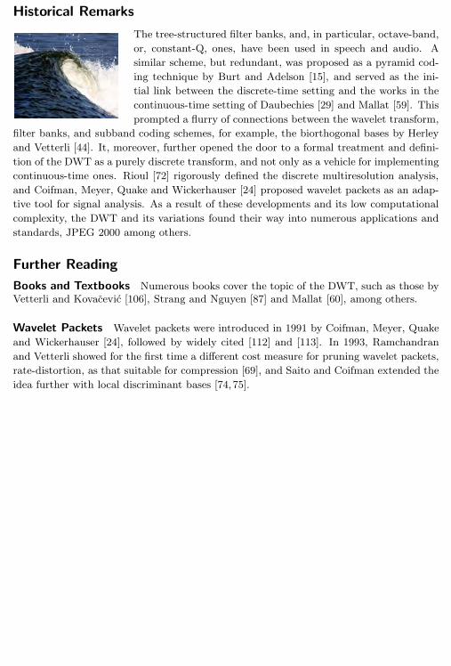
Historical Remarks 119
Historical Remarks
The tree-structured filter banks, and, in particular, octave-band,
or, constant-Q, ones, have been used in speech and audio. A
similar scheme, but redundant, was proposed as a pyramid cod-
ing technique by Burt and Adelson [15], and served as the ini-
tial link between the discrete-time setting and the works in the
continuous-time setting of Daubechies [29] and Mallat [59]. This
prompted a flurry of connections between the wavelet transform,
filter banks, and subband coding schemes, for example, the biorthogonal bases by Herley
and Vetterli [44]. It, moreover, further opened the door to a formal treatment and defini-
tion of the DWT as a purely discrete transform, and not only as a vehicle for implementing
continuous-time ones. Rioul [72] rigorously defined the discrete multiresolution analysis,
and Coifman, Meyer, Quake and Wickerhauser [24] proposed wavelet packets as an adap-
tive tool for signal analysis. As a result of these developments and its low computational
complexity, the DWT and its variations found their way into numerous applications and
standards, JPEG 2000 among others.
Further Reading
Books and Textbooks Numerous books cover the topic of the DWT, such as those byVetterli and Kovacevic [106], Strang and Nguyen [87] and Mallat [60], among others.
Wavelet Packets Wavelet packets were introduced in 1991 by Coifman, Meyer, Quake
and Wickerhauser [24], followed by widely cited [112] and [113]. In 1993, Ramchandran
and Vetterli showed for the first time a different cost measure for pruning wavelet packets,
rate-distortion, as that suitable for compression [69], and Saito and Coifman extended the
idea further with local discriminant bases [74,75].
Chapter 4
Local Fourier and Wavelet
Frames on Sequences
Contents
4.1 Introduction 122
4.2 Finite-Dimensional Frames 133
4.3 Oversampled Filter Banks 151
4.4 Local Fourier Frames 158
4.5 Wavelet Frames 165
4.6 Computational Aspects 171
Chapter at a Glance 173
Historical Remarks 174
Further Reading 174
Redundancy is a common tool in our daily lives; it helps remove doubt oruncertainty. Redundant signal representations follow the same idea to create ro-bustness. Given a sequence, we often represent it in another domain where itscharacteristics are more readily apparent in the expansion coefficients. If the repre-sentation in that other domain is achieved via a basis, corruption or loss of expansioncoefficients can be serious. If, on the other hand, that representation is achievedvia a redundant representation, such problems can be avoided.
As introduced in Chapter 2, Section 2.5.4, the redundant counterpart of basesare called frames. Frames are the topic of the present chapter. The building blocksof a representation can be seen as words in a dictionary; while a basis uses a min-imum number of such words, a frame uses an overcomplete set. This is similar tomultiple words with slight variations for similar concepts, allowing for very shortsentences describing complex ideas.25 While in most of the previous chapters, ouremphasis was on finding the best expansion/representation vectors (Fourier, wavelet,etc.), frames allow us even more freedom; not only do we look for the best expan-sion, we can also look for the best expansion coefficients given a fixed expansionand under desired constraints (sparsity as one example). This freedom is due to
25As the urban legend goes, Eskimos have a hundred words for snow.
121
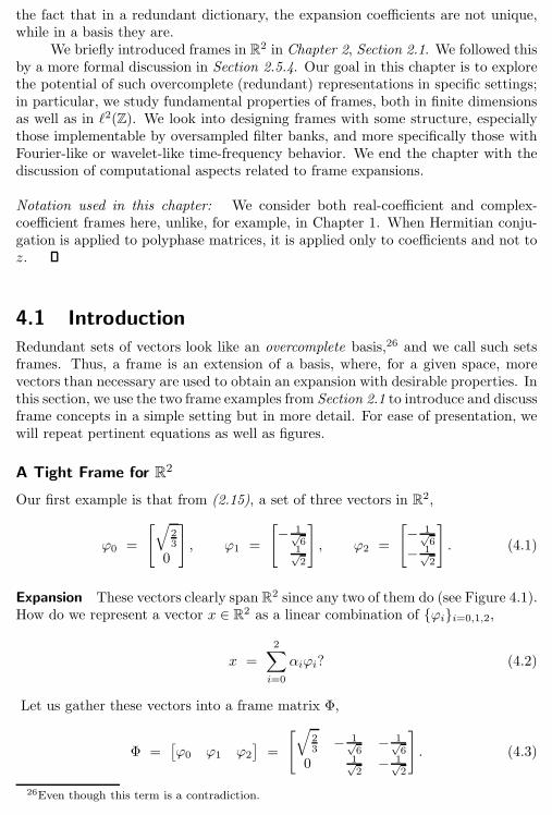
122 Chapter 4. Local Fourier and Wavelet Frames on Sequences
the fact that in a redundant dictionary, the expansion coefficients are not unique,while in a basis they are.
We briefly introduced frames in R2 in Chapter 2, Section 2.1. We followed thisby a more formal discussion in Section 2.5.4. Our goal in this chapter is to explorethe potential of such overcomplete (redundant) representations in specific settings;in particular, we study fundamental properties of frames, both in finite dimensionsas well as in ℓ2(Z). We look into designing frames with some structure, especiallythose implementable by oversampled filter banks, and more specifically those withFourier-like or wavelet-like time-frequency behavior. We end the chapter with thediscussion of computational aspects related to frame expansions.
Notation used in this chapter: We consider both real-coefficient and complex-coefficient frames here, unlike, for example, in Chapter 1. When Hermitian conju-gation is applied to polyphase matrices, it is applied only to coefficients and not toz.
4.1 Introduction
Redundant sets of vectors look like an overcomplete basis,26 and we call such setsframes. Thus, a frame is an extension of a basis, where, for a given space, morevectors than necessary are used to obtain an expansion with desirable properties. Inthis section, we use the two frame examples from Section 2.1 to introduce and discussframe concepts in a simple setting but in more detail. For ease of presentation, wewill repeat pertinent equations as well as figures.
A Tight Frame for R2
Our first example is that from (2.15), a set of three vectors in R2,
ϕ0 =
[√23
0
], ϕ1 =
[− 1√
61√2
], ϕ2 =
[− 1√
6
− 1√2
]. (4.1)
Expansion These vectors clearly span R2 since any two of them do (see Figure 4.1).How do we represent a vector x ∈ R2 as a linear combination of ϕii=0,1,2,
x =2∑
i=0
αiϕi? (4.2)
Let us gather these vectors into a frame matrix Φ,
Φ =[ϕ0 ϕ1 ϕ2
]=
[√23 − 1√
6− 1√
6
0 1√2− 1√
2
]. (4.3)
26Even though this term is a contradiction.
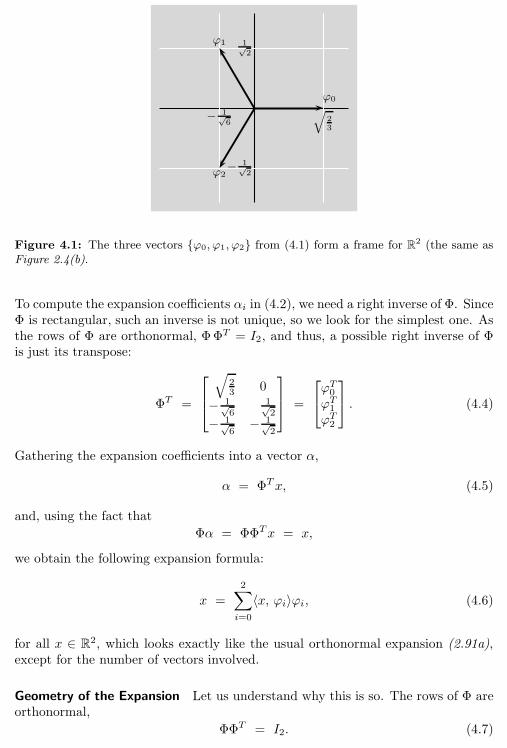
4.1. Introduction 123
√23
ϕ0
1√2
ϕ1
− 1√6
− 1√2ϕ2
Figure 4.1: The three vectors ϕ0, ϕ1, ϕ2 from (4.1) form a frame for R2 (the same as
Figure 2.4(b).
To compute the expansion coefficients αi in (4.2), we need a right inverse of Φ. SinceΦ is rectangular, such an inverse is not unique, so we look for the simplest one. Asthe rows of Φ are orthonormal, ΦΦT = I2, and thus, a possible right inverse of Φis just its transpose:
ΦT =
√23 0
− 1√6
1√2
− 1√6− 1√
2
=
ϕT0ϕT1ϕT2
. (4.4)
Gathering the expansion coefficients into a vector α,
α = ΦTx, (4.5)
and, using the fact that
Φα = ΦΦTx = x,
we obtain the following expansion formula:
x =
2∑
i=0
〈x, ϕi〉ϕi, (4.6)
for all x ∈ R2, which looks exactly like the usual orthonormal expansion (2.91a),except for the number of vectors involved.
Geometry of the Expansion Let us understand why this is so. The rows of Φ areorthonormal,
ΦΦT = I2. (4.7)
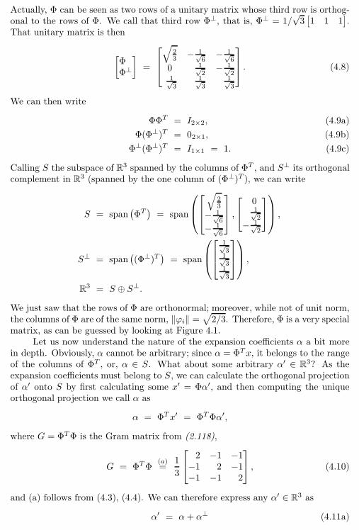
124 Chapter 4. Local Fourier and Wavelet Frames on Sequences
Actually, Φ can be seen as two rows of a unitary matrix whose third row is orthog-onal to the rows of Φ. We call that third row Φ⊥, that is, Φ⊥ = 1/
√3[1 1 1
].
That unitary matrix is then
[ΦΦ⊥
]=
√23 − 1√
6− 1√
6
0 1√2− 1√
21√3
1√3
1√3
. (4.8)
We can then write
ΦΦT = I2×2, (4.9a)
Φ(Φ⊥)T = 02×1, (4.9b)
Φ⊥(Φ⊥)T = I1×1 = 1. (4.9c)
Calling S the subspace of R3 spanned by the columns of ΦT , and S⊥ its orthogonalcomplement in R3 (spanned by the one column of (Φ⊥)T ), we can write
S = span(ΦT)
= span
√23
− 1√6
− 1√6
,
01√2
− 1√2
,
S⊥ = span((Φ⊥)T
)= span
1√31√31√3
,
R3 = S ⊕ S⊥.
We just saw that the rows of Φ are orthonormal; moreover, while not of unit norm,the columns of Φ are of the same norm, ‖ϕi‖ =
√2/3. Therefore, Φ is a very special
matrix, as can be guessed by looking at Figure 4.1.Let us now understand the nature of the expansion coefficients α a bit more
in depth. Obviously, α cannot be arbitrary; since α = ΦTx, it belongs to the rangeof the columns of ΦT , or, α ∈ S. What about some arbitrary α′ ∈ R3? As theexpansion coefficients must belong to S, we can calculate the orthogonal projectionof α′ onto S by first calculating some x′ = Φα′, and then computing the uniqueorthogonal projection we call α as
α = ΦTx′ = ΦTΦα′,
where G = ΦTΦ is the Gram matrix from (2.118),
G = ΦTΦ(a)=
1
3
2 −1 −1−1 2 −1−1 −1 2
, (4.10)
and (a) follows from (4.3), (4.4). We can therefore express any α′ ∈ R3 as
α′ = α+ α⊥ (4.11a)
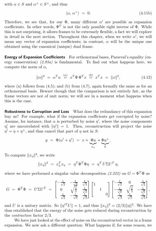
4.1. Introduction 125
with α ∈ S and α⊥ ∈ S⊥, and thus
〈α, α⊥〉 = 0. (4.11b)
Therefore, we see that, for our Φ, many different α′ are possible as expansioncoefficients. In other words, ΦT is not the only possible right inverse of Φ. Whilethis is not surprising, it allows frames to be extremely flexible, a fact we will explorein detail in the next section. Throughout this chapter, when we write α′, we willmean any vector of expansion coefficients; in contrast, α will be the unique oneobtained using the canonical (unique) dual frame.
Energy of Expansion Coefficients For orthonormal bases, Parseval’s equality (en-ergy conservation) (2.93a) is fundamental. To find out what happens here, wecompute the norm of α,
‖α‖2 = αTα(a)= xTΦΦTx
(b)= xTx = ‖x‖2, (4.12)
where (a) follows from (4.5); and (b) from (4.7), again formally the same as for anorthonormal basis. Beware though that the comparison is not entirely fair, as theframe vectors are not of unit norm; we will see in a moment what happens whenthis is the case.
Robustness to Corruption and Loss What does the redundancy of this expansionbuy us? For example, what if the expansion coefficients get corrupted by noise?Assume, for instance, that α is perturbed by noise η′, where the noise componentsη′iare uncorrelated with ‖η′‖ = 1. Then, reconstruction will project the noise
η′ = η + η⊥, and thus cancel that part of η not in S:
y = Φ(α′ + η′) = x+ Φη︸︷︷︸xη
+Φη⊥︸︷︷︸0
.
To compute ‖xη‖2, we write
‖xη‖2 = xTηxη = ηTΦTΦη = ηT UΣUT η,
where we have performed a singular value decomposition (2.222) on G = ΦTΦ as
G = ΦTΦ = UΣUT =
− 1√
2− 1√
61√3
0√
23
1√3
1√2− 1√
61√3
1
10
− 1√
20 1√
2
− 1√6
√23 − 1√
61√3
1√3
1√3
,
and U is a unitary matrix. So ‖η′TU‖ = 1, and thus ‖xη‖2 = (2/3)‖η‖2. We havethus established that the energy of the noise gets reduced during reconstruction bythe contraction factor 2/3.
We have just looked at the effect of noise on the reconstructed vector in a frameexpansion. We now ask a different question: What happens if, for some reason, we
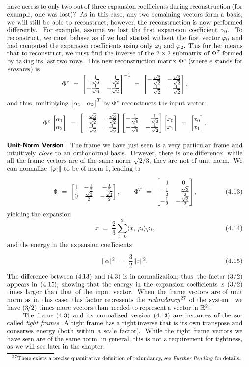
126 Chapter 4. Local Fourier and Wavelet Frames on Sequences
have access to only two out of three expansion coefficients during reconstruction (forexample, one was lost)? As in this case, any two remaining vectors form a basis,we will still be able to reconstruct; however, the reconstruction is now performeddifferently. For example, assume we lost the first expansion coefficient α0. Toreconstruct, we must behave as if we had started without the first vector ϕ0 andhad computed the expansion coefficients using only ϕ1 and ϕ2. This further meansthat to reconstruct, we must find the inverse of the 2 × 2 submatrix of ΦT formedby taking its last two rows. This new reconstruction matrix Φe (where e stands forerasures) is
Φe =
[− 1√
61√2
− 1√6− 1√
2
]−1
=
[−
√3√2−
√3√2
1√2− 1√
2
],
and thus, multiplying[α1 α2
]T
by Φe reconstructs the input vector:
Φe[α1
α2
]=
[−
√3√2−
√3√2
1√2− 1√
2
][− 1√
61√2
− 1√6− 1√
2
][x0x1
]=
[x0x1
].
Unit-Norm Version The frame we have just seen is a very particular frame andintuitively close to an orthonormal basis. However, there is one difference: whileall the frame vectors are of the same norm
√2/3, they are not of unit norm. We
can normalize ‖ϕi‖ to be of norm 1, leading to
Φ =
[1 − 1
2 − 12
0√32 −
√32
], ΦT =
1 0
− 12
√32
− 12 −
√32
, (4.13)
yielding the expansion
x =2
3
2∑
i=0
〈x, ϕi〉ϕi, (4.14)
and the energy in the expansion coefficients
‖α‖2 =3
2‖x‖2. (4.15)
The difference between (4.13) and (4.3) is in normalization; thus, the factor (3/2)appears in (4.15), showing that the energy in the expansion coefficients is (3/2)times larger than that of the input vector. When the frame vectors are of unitnorm as in this case, this factor represents the redundancy27 of the system—wehave (3/2) times more vectors than needed to represent a vector in R2.
The frame (4.3) and its normalized version (4.13) are instances of the so-called tight frames. A tight frame has a right inverse that is its own transpose andconserves energy (both within a scale factor). While the tight frame vectors wehave seen are of the same norm, in general, this is not a requirement for tightness,as we will see later in the chapter.
27There exists a precise quantitative definition of redundancy, see Further Reading for details.
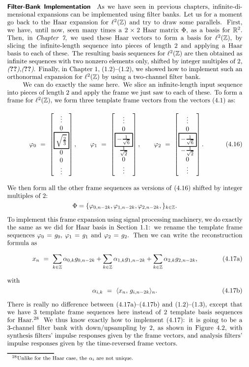
4.1. Introduction 127
Filter-Bank Implementation As we have seen in previous chapters, infinite-di-mensional expansions can be implemented using filter banks. Let us for a momentgo back to the Haar expansion for ℓ2(Z) and try to draw some parallels. First,we have, until now, seen many times a 2 × 2 Haar matrix Φ, as a basis for R
2.Then, in Chapter 7, we used these Haar vectors to form a basis for ℓ2(Z), byslicing the infinite-length sequence into pieces of length 2 and applying a Haarbasis to each of these. The resulting basis sequences for ℓ2(Z) are then obtained asinfinite sequences with two nonzero elements only, shifted by integer multiples of 2,(??),(??). Finally, in Chapter 1, (1.2)–(1.2), we showed how to implement such anorthonormal expansion for ℓ2(Z) by using a two-channel filter bank.
We can do exactly the same here. We slice an infinite-length input sequenceinto pieces of length 2 and apply the frame we just saw to each of these. To form aframe for ℓ2(Z), we form three template frame vectors from the vectors (4.1) as:
ϕ0 =
...0√
23
00...
, ϕ1 =
...0
− 1√6
1√2
0...
, ϕ2 =
...0
− 1√6
− 1√2
0...
. (4.16)
We then form all the other frame sequences as versions of (4.16) shifted by integermultiples of 2:
Φ = ϕ0,n−2k, ϕ1,n−2k, ϕ2,n−2k, k∈Z.
To implement this frame expansion using signal processing machinery, we do exactlythe same as we did for Haar basis in Section 1.1: we rename the template framesequences ϕ0 = g0, ϕ1 = g1 and ϕ2 = g2. Then we can write the reconstructionformula as
xn =∑
k∈Z
α0,kg0,n−2k +∑
k∈Z
α1,kg1,n−2k +∑
k∈Z
α2,kg2,n−2k, (4.17a)
with
αi,k = 〈xn, gi,n−2k〉n. (4.17b)
There is really no difference between (4.17a)–(4.17b) and (1.2)–(1.3), except thatwe have 3 template frame sequences here instead of 2 template basis sequencesfor Haar.28 We thus know exactly how to implement (4.17): it is going to be a3-channel filter bank with down/upsampling by 2, as shown in Figure 4.2, withsynthesis filters’ impulse responses given by the frame vectors, and analysis filters’impulse responses given by the time-reversed frame vectors.
28Unlike for the Haar case, the αi are not unique.
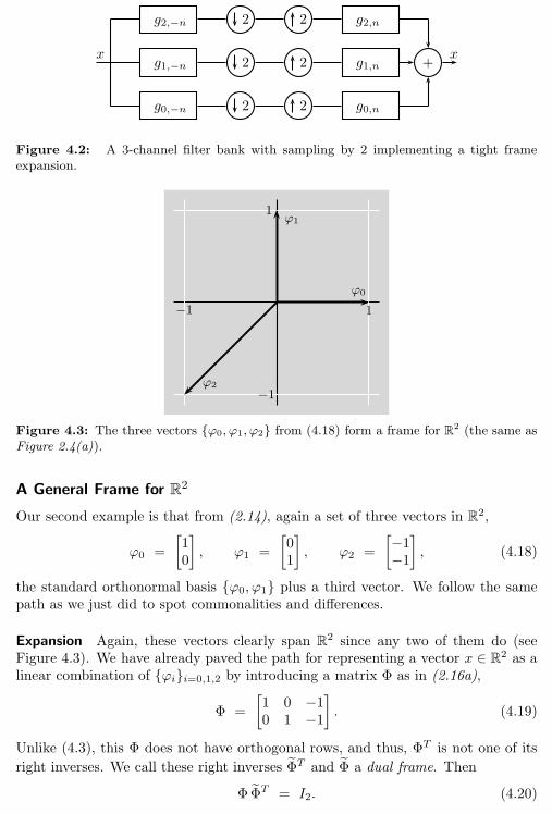
128 Chapter 4. Local Fourier and Wavelet Frames on Sequences
x
g2,−n
g1,−n
g0,−n
2
2
2
2
2
2
g2,n
g1,n
g0,n
+x
Figure 4.2: A 3-channel filter bank with sampling by 2 implementing a tight frameexpansion.
1
ϕ0
1ϕ1
−1
−1ϕ2
Figure 4.3: The three vectors ϕ0, ϕ1, ϕ2 from (4.18) form a frame for R2 (the same asFigure 2.4(a)).
A General Frame for R2
Our second example is that from (2.14), again a set of three vectors in R2,
ϕ0 =
[10
], ϕ1 =
[01
], ϕ2 =
[−1−1
], (4.18)
the standard orthonormal basis ϕ0, ϕ1 plus a third vector. We follow the samepath as we just did to spot commonalities and differences.
Expansion Again, these vectors clearly span R2 since any two of them do (see
Figure 4.3). We have already paved the path for representing a vector x ∈ R2 as alinear combination of ϕii=0,1,2 by introducing a matrix Φ as in (2.16a),
Φ =
[1 0 −10 1 −1
]. (4.19)
Unlike (4.3), this Φ does not have orthogonal rows, and thus, ΦT is not one of its
right inverses. We call these right inverses ΦT and Φ a dual frame. Then
Φ ΦT = I2. (4.20)
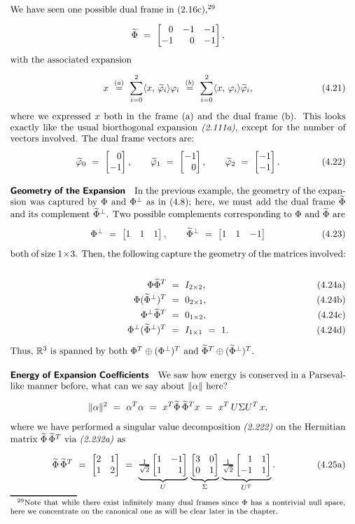
4.1. Introduction 129
We have seen one possible dual frame in (2.16c),29
Φ =
[0 −1 −1−1 0 −1
],
with the associated expansion
x(a)=
2∑
i=0
〈x, ϕi〉ϕi(b)=
2∑
i=0
〈x, ϕi〉ϕi, (4.21)
where we expressed x both in the frame (a) and the dual frame (b). This looksexactly like the usual biorthogonal expansion (2.111a), except for the number ofvectors involved. The dual frame vectors are:
ϕ0 =
[0−1
], ϕ1 =
[−10
], ϕ2 =
[−1−1
]. (4.22)
Geometry of the Expansion In the previous example, the geometry of the expan-sion was captured by Φ and Φ⊥ as in (4.8); here, we must add the dual frame Φ
and its complement Φ⊥. Two possible complements corresponding to Φ and Φ are
Φ⊥ =[1 1 1
], Φ⊥ =
[1 1 −1
](4.23)
both of size 1×3. Then, the following capture the geometry of the matrices involved:
ΦΦT = I2×2, (4.24a)
Φ(Φ⊥)T = 02×1, (4.24b)
Φ⊥ΦT = 01×2, (4.24c)
Φ⊥(Φ⊥)T = I1×1 = 1. (4.24d)
Thus, R3 is spanned by both ΦT ⊕ (Φ⊥)T and ΦT ⊕ (Φ⊥)T .
Energy of Expansion Coefficients We saw how energy is conserved in a Parseval-like manner before, what can we say about ‖α‖ here?
‖α‖2 = αTα = xT Φ ΦTx = xT UΣUT x,
where we have performed a singular value decomposition (2.222) on the Hermitian
matrix Φ ΦT via (2.232a) as
Φ ΦT =
[2 11 2
]= 1√
2
[1 −11 1
]
︸ ︷︷ ︸U
[3 00 1
]
︸ ︷︷ ︸Σ
1√2
[1 1−1 1
]
︸ ︷︷ ︸UT
. (4.25a)
29Note that while there exist infinitely many dual frames since Φ has a nontrivial null space,here we concentrate on the canonical one as will be clear later in the chapter.
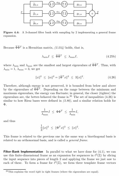
130 Chapter 4. Local Fourier and Wavelet Frames on Sequences
x
g2,n
g1,n
g0,n
2
2
2
α2
α1
α0
2
2
2
g2,n
g1,n
g0,n
+x
Figure 4.4: A 3-channel filter bank with sampling by 2 implementing a general frameexpansion.
Because ΦΦT is a Hermitian matrix, (2.234) holds, that is,
λminI ≤ ΦΦT ≤ λmaxI, (4.25b)
where λmin and λmax are the smallest and largest eigenvalues of ΦΦT . Thus, withλmin = 1, λmax = 3, we get
‖x‖2 ≤ ‖α‖2 = ‖ΦTx‖2 ≤ 3‖x‖2. (4.26)
Therefore, although energy is not preserved, it is bounded from below and aboveby the eigenvalues of ΦΦT . Depending on the range between the minimum andmaximum eigenvalues, the energy can fluctuate; in general, the closer (tighter) theeigenvalues are, the better-behaved the frame is.30 The set of inequalities (4.26) issimilar to how Riesz bases were defined in (2.86), and a similar relation holds forΦ,
1
λmaxI ≤ ΦΦT ≤ 1
λminI,
and thus
1
3‖x‖2 ≤ ‖ΦTx‖2 ≤ ‖x‖2.
This frame is related to the previous one in the same way a biorthogonal basis isrelated to an orthonormal basis, and is called a general frame.
Filter-Bank Implementation In parallel to what we have done for (4.1), we canuse this finite-dimensional frame as an expansion for sequences in ℓ2(Z) by slicingthe input sequence into pieces of length 2 and applying the frame we just saw toeach of these. To form a frame for ℓ2(Z), we form three template frame vectors
30This explains the word tight in tight frames (where the eigenvalues are equal).
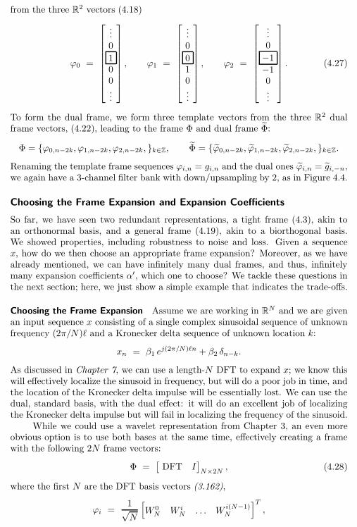
4.1. Introduction 131
from the three R2 vectors (4.18)
ϕ0 =
...0
100...
, ϕ1 =
...0
010...
, ϕ2 =
...0
−1−10...
. (4.27)
To form the dual frame, we form three template vectors from the three R2 dualframe vectors, (4.22), leading to the frame Φ and dual frame Φ:
Φ = ϕ0,n−2k, ϕ1,n−2k, ϕ2,n−2k, k∈Z, Φ = ϕ0,n−2k, ϕ1,n−2k, ϕ2,n−2k, k∈Z.
Renaming the template frame sequences ϕi,n = gi,n and the dual ones ϕi,n = gi,−n,we again have a 3-channel filter bank with down/upsampling by 2, as in Figure 4.4.
Choosing the Frame Expansion and Expansion Coefficients
So far, we have seen two redundant representations, a tight frame (4.3), akin toan orthonormal basis, and a general frame (4.19), akin to a biorthogonal basis.We showed properties, including robustness to noise and loss. Given a sequencex, how do we then choose an appropriate frame expansion? Moreover, as we havealready mentioned, we can have infinitely many dual frames, and thus, infinitelymany expansion coefficients α′, which one to choose? We tackle these questions inthe next section; here, we just show a simple example that indicates the trade-offs.
Choosing the Frame Expansion Assume we are working in RN and we are givenan input sequence x consisting of a single complex sinusoidal sequence of unknownfrequency (2π/N)ℓ and a Kronecker delta sequence of unknown location k:
xn = β1 ej(2π/N)ℓn + β2 δn−k.
As discussed in Chapter 7, we can use a length-N DFT to expand x; we know thiswill effectively localize the sinusoid in frequency, but will do a poor job in time, andthe location of the Kronecker delta impulse will be essentially lost. We can use thedual, standard basis, with the dual effect: it will do an excellent job of localizingthe Kronecker delta impulse but will fail in localizing the frequency of the sinusoid.
While we could use a wavelet representation from Chapter 3, an even moreobvious option is to use both bases at the same time, effectively creating a framewith the following 2N frame vectors:
Φ =[DFT I
]N×2N
, (4.28)
where the first N are the DFT basis vectors (3.162),
ϕi =1√N
[W 0N
W i
N. . . W
i(N−1)N
]T
,
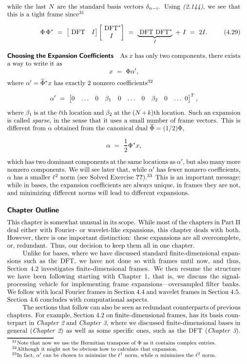
132 Chapter 4. Local Fourier and Wavelet Frames on Sequences
while the last N are the standard basis vectors δn−i. Using (2.144), we see thatthis is a tight frame since31
ΦΦ∗ =[DFT I
] [ DFT∗
I
]= DFT DFT∗︸ ︷︷ ︸
I
+ I = 2I. (4.29)
Choosing the Expansion Coefficients As x has only two components, there existsa way to write it as
x = Φα′,
where α′ = Φ∗x has exactly 2 nonzero coefficients32
α′ =[0 . . . 0 β1 0 . . . 0 β2 0 . . . 0
]T
,
where β1 is at the ℓth location and β2 at the (N +k)th location. Such an expansionis called sparse, in the sense that it uses a small number of frame vectors. This isdifferent from α obtained from the canonical dual Φ = (1/2)Φ,
α =1
2Φ∗x,
which has two dominant components at the same locations as α′, but also many morenonzero components. We will see later that, while α′ has fewer nonzero coefficients,α has a smaller ℓ2 norm (see Solved Exercise ??).33 This is an important message;while in bases, the expansion coefficients are always unique, in frames they are not,and minimizing different norms will lead to different expansions.
Chapter Outline
This chapter is somewhat unusual in its scope. While most of the chapters in Part IIdeal either with Fourier- or wavelet-like expansions, this chapter deals with both.However, there is one important distinction: these expansions are all overcomplete,or, redundant. Thus, our decision to keep them all in one chapter.
Unlike for bases, where we have discussed standard finite-dimensional expan-sions such as the DFT, we have not done so with frames until now, and thus,Section 4.2 investigates finite-dimensional frames. We then resume the structurewe have been following starting with Chapter 1, that is, we discuss the signal-processing vehicle for implementing frame expansions—oversampled filter banks.We follow with local Fourier frames in Section 4.4 and wavelet frames in Section 4.5.Section 4.6 concludes with computational aspects.
The sections that follow can also be seen as redundant counterparts of previouschapters. For example, Section 4.2 on finite-dimensional frames, has its basis coun-terpart in Chapter 2 and Chapter 3, where we discussed finite-dimensional bases ingeneral (Chapter 2) as well as some specific ones, such as the DFT (Chapter 3).
31Note that now we use the Hermitian transpose of Φ as it contains complex entries.32Although it might not be obvious how to calculate that expansion.33In fact, α′ can be chosen to minimize the ℓ1 norm, while α minimizes the ℓ2 norm.
4.2. Finite-Dimensional Frames 133
Section 4.3 on oversampled filter banks has its basis (critically-sampled filter bank)counterpart in Chapter 1 (two-channel critically-sampled filter banks), Chapter 2(N -channel critically-sampled filter banks) and Chapter 3 (tree-structured critically-sampled filter banks). Section 4.4 on local Fourier frames has its basis counterpartin Chapter 2 (local Fourier bases on sequences), while Section 4.5 on wavelet frameshas its basis counterpart in Chapter 3 (wavelet bases on sequences). Thus, this chap-ter also plays a unifying role in summarizing concepts on expansions of sequences.The two chapters that follow this one will deal with functions instead of sequences.
4.2 Finite-Dimensional Frames
We have just seen examples showing that finite-dimensional overcomplete sets ofvectors have properties similar to orthonormal and/or biorthogonal bases. We willnow look into general properties of such finite-dimensional frames in CN , with theunderstanding that RN is just a special case. We start with tight frames and followwith general frames. Since the representation in a frame is in general nonunique,we discuss how to compute expansion coefficients, and point out that, dependingon which norm is minimized, different solutions are obtained.
Finite-dimensional frames are represented via rectangular matrices; thus, allthe material in this section is basic linear algebra. We use this simplicity to developthe geometric intuition to be carried to infinite-dimensional frames that follow.
4.2.1 Tight Frames for CN
We work in a finite-dimensional space CN , where, a set of vectors Φ = ϕiM−1i=0 ,
M > N , is a frame represented (similarly to (4.3) and (4.19)) by the frame matrixΦ as
Φ =[ϕ0 ϕ1 . . . ϕM−1
]N×M . (4.30)
Assume that the rank(Φ) = N , that is, the column range of Φ is CN . Thus, anyx ∈ C
N can be written as a nonunique linear combination of ϕi’s.We impose a further constraint and start with frames that satisfy a Parseval-
like equality:
Definition 4.1 (Tight frame) A family Φ = ϕiM−1i=0 in CN is called a tight
frame, or, λ-tight frame when there exists a constant 0 < λ <∞ called the framebound, such that for all x ∈ CN ,
λ‖x‖2 =
M−1∑
i=0
|〈x, ϕi〉|2 = ‖Φ∗x‖2. (4.31)
134 Chapter 4. Local Fourier and Wavelet Frames on Sequences
Expansion
Equation (4.31) has a number of consequences. First, it means that
ΦΦ∗ = λI. (4.32)
Thus, Φ∗ is a right inverse of Φ. Calling Φ the dual frame as before, we see that
Φ =1
λΦ. (4.33)
Then:
x = Φα, α =1
λΦ∗x, (4.34a)
x =1
λ
M−1∑
i=0
〈x, ϕi〉ϕi. (4.34b)
This looks very similar to an orthonormal basis expansion, except for the scalingfactor (1/λ) and the fact that Φ = ϕiM−1
i=0 cannot be a basis since ϕi are notlinearly independent. We can pull the factor (1/λ) into the sum and renormalizethe frame vectors as ϕ′
i= (1/
√λ)ϕi leading to the expression that formally looks
identical to that of an orthonormal basis expansion:
x =
M−1∑
i=0
〈x, ϕ′i〉ϕ′i. (4.35)
We have already seen an example of such a renormalization in (4.1) and (4.13). Aframe normalized so that λ = 1 is called a Parseval tight frame or a 1-tight frame.
The expression for x is what is typically called a reconstruction or a repre-sentation of a sequence, or, in filter banks, synthesis, while the expression for theexpansion coefficients α is a decomposition, or, analysis in filter banks.
In the discussion above, we said nothing about the norms of the individualframe vectors. Since the analysis computes inner products αi = 〈x, ϕi〉, it oftenmakes sense for all ϕi to have the same norm, leading to an equal-norm frame (whichmay not be tight). When we combine equal norm with tightness, we get a framethat acts every bit like an orthonormal basis, except for the redundancy. That is,all inner products αi = 〈x, ϕi〉 are projections of x onto vectors of the same norm,allowing us to compare coefficients αi to each other. Moreover, because the frameis tight, the right inverse is simply its adjoint (within scaling). In finite dimensions,tightness corresponds to the rows of Φ being orthogonal. Because of this, it is hardin general to obtain an equal-norm frame starting from the tight one.
Geometry of the Expansion Let us explore the geometry of tight frames. Withthe frame matrix Φ as in (4.30), and as we did in (4.8), we introduce Φ⊥,
Φ⊥ =[ϕ⊥0 ϕ⊥
1 . . . ϕ⊥M−1
](M−N)×M (4.36)
4.2. Finite-Dimensional Frames 135
as one possible orthogonal complement of Φ in CM :
[ΦΦ⊥
]=
[ϕ0 ϕ1 . . . ϕM−1
ϕ⊥0 ϕ⊥
1 . . . ϕ⊥M−1
]
M×M(4.37)
that is, the rows of Φ⊥ are chosen to be orthogonal to the rows of Φ, orthogonal toeach other and of norm 1, or,
[ΦΦ⊥
] [Φ∗ (Φ⊥)∗
]=
[ΦΦ∗ Φ(Φ⊥)∗
Φ⊥Φ∗ Φ⊥(Φ⊥)∗
]
=
[IN×N 0
0 I(M−N)×(M−N)
]= IM×M . (4.38)
Note that each vector ϕi is in CN , while each vector ϕ⊥i
is in CM−N . We canrewrite (4.37) as
S = span(ΦT)⊂ C
M , (4.39a)
S⊥ = span((Φ⊥)T
)⊂ C
M , (4.39b)
CM = S ⊕ S⊥, (4.39c)
and, because of (4.38),
ΦΦ∗ = IN×N , (4.40a)
Φ(Φ⊥)∗ = 0N×(M−N), (4.40b)
Φ⊥(Φ⊥)∗ = I(M−N)×(M−N). (4.40c)
A vector of expansion coefficients α′ ∈ CM can be written as
α′ = α+ α⊥ (4.41a)
with α ∈ S and α⊥ ∈ S⊥, and thus
〈α, α⊥〉 = 0, (4.41b)
as we have already seen in the simple example in the previous section, (4.11b).
Relation to Orthonormal Bases
We now look into connections between tight frames and orthonormal bases.
Theorem 4.2 A 1-tight frame with unit-norm vectors is an orthonormal basis.
Proof. For a tight frame expansion with λ = 1,
T = ΦΦ∗ = I,
136 Chapter 4. Local Fourier and Wavelet Frames on Sequences
and thus, all the eigenvalues of T are equal to 1. Using one of the useful frame relationswe introduce later in (4.64a),
N(a)=
N−1∑
j=0
λj(b)=
M−1∑
i=0
‖ϕi‖2(c)= M,
where (a) follows from all eigenvalues being equal to 1; (b) from (4.64a); and (c) fromall frame vectors being of unit norm. We get that M = N , and thus, our frame is anorthonormal basis.
In this result, we see once more the tantalizing connection between tight frames andorthonormal bases. In fact, even more is true: tight frames and orthonormal basesarise from the minimization of the same quantity called the frame potential :
FP(Φ) =
M−1∑
i,j=0
|〈ϕi, ϕj〉|2. (4.42)
In fact, minimizing the frame potential has two possible outcomes:
(i) When M ≤ N , the minimum value of the frame potential is
FP(Φ) = N,
achieved when Φ is an orthonormal set.
(ii) When M > N , the minimum value of the frame potential is
FP(Φ) =M2
N,
achieved when Φ is a unit-norm tight frame.34
This tells us that unit-norm tight frames are a natural extension of orthonormalbases, that is, the theorem formalizes the intuitive notion that unit-norm tightframes are a generalization of orthonormal bases. Moreover, both orthonormal basesand unit-norm tight frames are results of the minimization of the frame potential,with different parameters (number of elements equal/larger than the dimension ofthe space). We give pointers to more details on this topic in Further Reading.
Example 4.1 (Tight frames and orthonormal bases) We illustrate thisresult with an example. Fix N = 2.
(i) We first consider the case when M = N = 2. Then, we have two vectorsonly, ϕ0 and ϕ1, both on the unit circle. According to (4.42), the framepotential is
FP(ϕ0, ϕ1) = ‖ϕ0‖2+‖ϕ1‖2+2|〈ϕ0, ϕ1〉|2(a)= 2(1+|〈ϕ0, ϕ1〉|2), (4.43)
where (a) follows from ϕ0, ϕ1, being of unit norm. The above expression isminimized when 〈ϕ0, ϕ1〉 = 0, that is, when ϕ0 and ϕ1 form an orthonormalbasis. In that case, the minimum of the frame potential is FP = 2 = N .
34This lower bound for frames is known as Welch bound arising when minimizing interuserinterference in a CDMA system (see Further Reading for pointers).
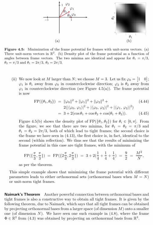
4.2. Finite-Dimensional Frames 137
1
−1 1
ϕ0
ϕ1
ϕ2
θ1θ2
0 Π
32Π
3Π
0
Π
3
2Π
3
Π
θ1
θ 2
(a) (b)
Figure 4.5: Minimization of the frame potential for frames with unit-norm vectors. (a)Three unit-norm vectors in R
2. (b) Density plot of the frame potential as a function ofangles between frame vectors. The two minima are identical and appear for θ1 = π/3,θ2 = π/3 and θ1 = 2π/3, θ2 = 2π/3.
(ii) We now look atM larger thanN ; we chooseM = 3. Let us fix ϕ0 =[1 0
];
ϕ1 is θ1 away from ϕ0 in counterclockwise direction; ϕ2 is θ2 away fromϕ1 in counterclockwise direction (see Figure 4.5(a)). The frame potentialis now
FP(θ1, θ2) = ‖ϕ0‖2 + ‖ϕ1‖2 + ‖ϕ2‖2 + (4.44)
2(|〈ϕ0, ϕ1〉|2 + |〈ϕ0, ϕ2〉|2 + |〈ϕ1, ϕ2〉|2)= 3 + 2(cos θ1 + cos θ2 + cos(θ1 + θ2)). (4.45)
Figure 4.5(b) shows the density plot of FP(θ1, θ2) for θi ∈ [0, π]. Fromthe figure, we see that there are two minima, for θ1 = θ2 = π/3 andθ1 = θ2 = 2π/3, both of which lead to tight frames; the second choice isthe frame we have seen in (4.13), the first choice is, in fact, identical to thesecond (within reflection). We thus see that the results of minimizing theframe potential in this case are tight frames, with the minimum of
FP(π3,π
3) = FP(2π
3, 2π
3) = 3 + 2(
1
4+
1
4+
1
4) =
9
2=
M2
N,
as per the theorem.
This simple example shows that minimizing the frame potential with differentparameters leads to either orthonormal sets (orthonormal bases when M = N)or unit-norm tight frames.
Naimark’s Theorem Another powerful connection between orthonormal bases andtight frames is also a constructive way to obtain all tight frames. It is given by thefollowing theorem, due to Naimark, which says that all tight frames can be obtainedby projecting orthonormal bases from a larger space (of dimensionM) onto a smallerone (of dimension N). We have seen one such example in (4.8), where the frameΦ ∈ R2 from (4.3) was obtained by projecting an orthonormal basis from R3.
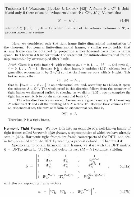
138 Chapter 4. Local Fourier and Wavelet Frames on Sequences
Theorem 4.3 (Naimark [3], Han & Larson [42]) A frame Φ ∈ CN is tightif and only if there exists an orthonormal basis Ψ ∈ CM , M ≥ N , such that
Φ∗ = Ψ[J ], (4.46)
where J ⊂ 0, 1, . . . , M − 1 is the index set of the retained columns of Ψ, aprocess known as seeding.
Here, we considered only the tight-frame finite-dimensional instantiation ofthe theorem. For general finite-dimensional frames, a similar result holds, thatis, any frame can be obtained by projecting a biorthogonal basis from a largerspace. In Theorem 4.8 we formulate the statement for infinite-dimensional framesimplementable by oversampled filter banks.
Proof. Given is a tight frame Φ, with columns ϕi, i = 0, 1, . . . , M − 1, and rows ψj ,j = 0, 1, . . . , N − 1. Because Φ is a tight frame, it satisfies (4.32); without loss ofgenerality, renormalize it by (1/
√λ) so that the frame we work with is 1-tight. This
further means that〈ψi, ψj〉 = δi−j ,
that is, ψ0, ψ1, . . . , ψN−1 is an orthonormal set, and, according to (4.39a), it spansthe subspace S ⊂ C
M . The whole proof in this direction follows from the geometry oftight frames we discussed earlier, by showing, as we did in (4.37), how to complete thetight frame matrix Φ to obtain an orthonormal basis Ψ∗.
The other direction is even easier. Assume we are given a unitary Ψ. Choose anyN columns of Ψ and call the resulting M ×N matrix Φ∗. Because these columns forman orthonormal set, the rows of Φ form an orthonormal set, that is,
ΦΦ∗ = I.
Therefore, Φ is a tight frame.
Harmonic Tight Frames We now look into an example of a well-known family oftight frames called harmonic tight frames, a representative of which we have alreadyseen in (4.3). Harmonic tight frames are frame counterparts of the DFT, and are,in fact, obtained from the DFT by seeding, a process defined in Theorem 4.3.
Specifically, to obtain harmonic tight frames, we start with the DFT matrixΨ = DFTM given in (3.161a) and delete its last (M −N) columns, yielding:
Φ =
1 1 1 . . . 1
1 WM W 2M
. . . WM−1M
1 W 2M
W 4M
. . . W2(M−1)M
......
.... . .
...
1 W(N−1)M
W(N−1)·2M
. . . W(N−1)(M−1)M
, (4.47a)
with the corresponding frame vectors
ϕi =[W 0M
W i
M. . . W
i(N−1)M
]T
, (4.47b)
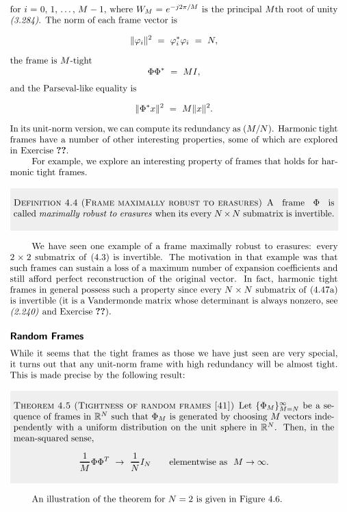
4.2. Finite-Dimensional Frames 139
for i = 0, 1, . . . , M − 1, where WM = e−j2π/M is the principal Mth root of unity(3.284). The norm of each frame vector is
‖ϕi‖2 = ϕ∗iϕi = N,
the frame is M -tightΦΦ∗ = MI,
and the Parseval-like equality is
‖Φ∗x‖2 = M‖x‖2.
In its unit-norm version, we can compute its redundancy as (M/N). Harmonic tightframes have a number of other interesting properties, some of which are exploredin Exercise ??.
For example, we explore an interesting property of frames that holds for har-monic tight frames.
Definition 4.4 (Frame maximally robust to erasures) A frame Φ iscalled maximally robust to erasures when its every N ×N submatrix is invertible.
We have seen one example of a frame maximally robust to erasures: every2 × 2 submatrix of (4.3) is invertible. The motivation in that example was thatsuch frames can sustain a loss of a maximum number of expansion coefficients andstill afford perfect reconstruction of the original vector. In fact, harmonic tightframes in general possess such a property since every N ×N submatrix of (4.47a)is invertible (it is a Vandermonde matrix whose determinant is always nonzero, see(2.240) and Exercise ??).
Random Frames
While it seems that the tight frames as those we have just seen are very special,it turns out that any unit-norm frame with high redundancy will be almost tight.This is made precise by the following result:
Theorem 4.5 (Tightness of random frames [41]) Let ΦM∞M=N be a se-quence of frames in RN such that ΦM is generated by choosing M vectors inde-pendently with a uniform distribution on the unit sphere in RN . Then, in themean-squared sense,
1
MΦΦT → 1
NIN elementwise as M →∞.
An illustration of the theorem for N = 2 is given in Figure 4.6.
140 Chapter 4. Local Fourier and Wavelet Frames on Sequences
-0.2
-0.1
0.1
0.2
M
∆00
-0.2
-0.1
0.1
0.2
M
∆01
-0.2
-0.1
0.1
0.2
M
∆10
-0.2
-0.1
0.1
0.2
M
∆11
Figure 4.6: Illustration of tightness of random frames for N = 2, andM = 2, 3 . . . , 1000.Since the convergence is elementwise, each graph plots the behavior ∆ij = [(1/M)ΦΦT −(1/2)I2]ij for i, j = 0, 1.
4.2.2 General Frames for CN
Tight frames are attractive the same way orthonormal bases are. They obey aParseval-like energy conservation equality, and the dual frame is equal to the frameitself (the right inverse of Φ is just its own Hermitian transpose, possibly withinscaling). Tightness, however, has sometimes to be relaxed, just as orthonormalitydoes (for example, when we wanted to design two-channel linear-phase filter banksin Chapter 1). Either a frame is given by a specific construction, and is not tight,or the constraints posed by tightness are too restrictive for a desired design.
Given a frame Φ as in (4.30) of rank(Φ) = N , we can find the canonical dual
frame Φ (formalized in Definition 4.7), also of size N × M , made of dual framevectors as
Φ = (ΦΦ∗)−1Φ, (4.48a)
=[ϕ0 ϕ1 . . . ϕM−1
]N×M , (4.48b)
ϕi = (ΦΦ∗)−1ϕi. (4.48c)
The above are all well-defined, since T = ΦΦ∗ is of rank N and can thus be in-verted. Therefore, Φ and Φ play the same roles for frames as their namesakes dofor biorthogonal bases, and, using (4.48a):
ΦΦ∗ = ΦΦ∗ (ΦΦ∗)−1 = IN , (4.49a)
ΦΦ∗ = (ΦΦ∗)−1 ΦΦ∗ = IN . (4.49b)
Note that the canonical dual frame Φ chosen here is a particular right inverse;we will formalize this in Definition 4.7. Note also that when Φ is tight, with thisdefinition of the dual, we indeed obtain Φ = Φ.
4.2. Finite-Dimensional Frames 141
Expansion
We know that Φ = ϕiM−1i=0 span CN , that is, any x ∈ CN can be written as
x =M−1∑
i=0
αiϕi (4.50a)
=
M−1∑
i=0
αiϕi, (4.50b)
both of which follow from (4.49) by writing
x(a)= ΦΦ∗x = Φα (4.51a)
(b)= ΦΦ∗x = Φα, (4.51b)
where (a) leads to (4.50a) and (b) to (4.50b), respectively. Again, these are recon-struction (representation) of a sequence, or, in filter banks, synthesis.
We have used αi and αi liberally, defining them implicitly. It comes as nosurprise that
αi = 〈x, ϕi〉 α = Φ∗x, (4.52a)
αi = 〈x, ϕi〉 α = Φ∗x; (4.52b)
they are interchangeable like the expansion expressions. As before, the expressionfor α is sometimes called decomposition (or, analysis, in filter banks).
Geometry of the Expansion Similarly to tight frames, let us explore the geometryof general frames. For tight frames, we dealt with Φ and Φ⊥ as in (4.30),(4.37);
here, we must add the dual frame Φ and its complement Φ⊥:
Φ Φ N ×MΦ⊥ Φ⊥ (M −N)×M
with, similarly to (4.38),
ΦΦ∗ = IN×N , (4.53a)
Φ(Φ⊥)∗ = 0N×(M−N), (4.53b)
Φ⊥Φ∗ = 0(M−N)×N , (4.53c)
Φ⊥(Φ⊥)∗ = I(M−N)×(M−N). (4.53d)
As in (4.39a), S is the subspace of CM spanned by the columns of Φ∗, while S⊥ is thesubspace of CM spanned by the columns of (Φ⊥)∗.35 We will see when discussingprojection operators shortly, that
span(Φ∗) = span(Φ∗), (4.54a)
span((Φ⊥)∗) = span((Φ⊥)∗), (4.54b)
35Note that the span(Φ∗) = span(ΦT ).
142 Chapter 4. Local Fourier and Wavelet Frames on Sequences
and thus, from now on, we will use that
S = span (Φ∗) . (4.55)
As before, an arbitrary vector of expansion coefficients α′ ∈ CM can be written as
α′ = α+ α⊥ (4.56a)
with α ∈ S and α⊥ ∈ S⊥, and thus
〈α, α⊥〉 = 0. (4.56b)
Frame Operator T When calculating the dual frame, the so-called canonical dualof Φ, the product ΦΦ∗ is central; we call it
TN×N = ΦΦ∗. (4.57)
It is a Hermitian and positive definite matrix (see (2.233), and thus, all of itseigenvalues are real and positive. According to (2.232a), T can be diagonalized as
T = ΦΦ∗ = UΛU∗, (4.58)
where Λ is a diagonal matrix of eigenvalues, and U a unitary matrix of eigenvectors.The largest λmax and smallest λmin eigenvalues play a special role. For tight frames,λmax = λmin = λ, and T is a scaled identity, T = λI, as it possesses a singleeigenvalue λ of multiplicity N .
Energy of Expansion Coefficients In the examples in the introduction as well asfor tight frames earlier, we have seen how the energy of the expansion coefficientsis conserved or bounded, (4.12), (4.26), and (4.31), respectively. We now look intoit for general frames by computing the energy of the expansion coefficients α as
‖α‖2 = α∗α(a)= x∗ΦΦ∗x
(b)= x∗ UΛU∗ x, (4.59)
where (a) follows from (4.51b) and (b) from (4.57). Thus, using (4.25b),
λmin‖x‖2 ≤ ‖α‖2 ≤ λmax‖x‖2. (4.60a)
Therefore, the energy, while not preserved, is bounded from below and above by theeigenvalues of T . How close (tight) these eigenvalues are will influence the qualityof the frame in question, as we will see later. The same argument above can berepeated for ‖α‖, leading to
1
λmax‖x‖2 ≤ ‖α‖2 ≤ 1
λmin‖x‖2. (4.60b)
Relation to Tight Frames Given a general frame Φ, we can easily transform itinto a tight frame Φ′. We do this by diagonalizing T as in (4.58). Then the tightframe is obtained as
Φ′ = UΛ−1/2U∗ Φ.
4.2. Finite-Dimensional Frames 143
Frame Operators
The pair of inequalities (4.60a) leads to an alternate definition of a frame, similarin spirit to Definition 2.43 for biorthogonal bases:
Definition 4.6 (Frame) A family Φ = ϕiM−1i=0 in CN is called a frame when
there exist two constants 0 < λmin ≤ λmax <∞, such that for all x ∈ CN ,
λmin‖x‖2 ≤M−1∑
i=0
|〈x, ϕi〉|2 ≤ λmax‖x‖2, (4.61)
where λmin, λmax are called lower and upper frame bounds.
Because of (4.60a), the frame bounds are clearly the eigenvalues of T as wehave seen previously. From the definition, we can also understand the meaning ofλ we have seen in (4.31); tight frames are obtained when the two frame bounds areequal, that is, when λmax = λmin = λ.
The operators we have seen so far are sometimes called: analysis frame oper-ator Φ∗, synthesis frame operator Φ, and frame operator T = ΦΦ∗. The analysisframe operator is one of many, as there exist infinitely many dual frames for a givenframe Φ. In our finite-dimensional setting, the analysis frame operator maps aninput x ∈ CN onto a subspace of CM , namely α = Φ∗x belongs to the subspace Sspanned by the columns of Φ∗ as we have seen in (4.55).36 These, together withother frame operators introduced shortly, are summarized in Table 4.1.
Given x ∈ CN , the frame operator T = ΦΦ∗ is a linear operator from CN toCN , guaranteed to be of full rank N since (4.61) ensures that λmin > 0. Also,
λminI ≤ T = ΦΦ∗ ≤ λmaxI. (4.62)
On the other hand, given x ∈ CM , the operator Φ∗Φ, which we have seenbefore as a projection operator (4.10) in our simple example, maps the input onto a
36Remember that S is spanned by either Φ∗ or Φ∗.
144 Chapter 4. Local Fourier and Wavelet Frames on Sequences
subspace S of CM . We called that operator a Gram operator in (2.118), G = Φ∗Φ:
G =
ϕ∗0
ϕ∗1...
ϕ∗M−1
[ϕ0 ϕ1 . . . ϕM−1
]
=
〈ϕ0, ϕ0〉 〈ϕ0, ϕ1〉 . . . 〈ϕ0, ϕM−1〉〈ϕ1, ϕ0〉 〈ϕ1, ϕ1〉 . . . 〈ϕ1, ϕM−1〉
......
. . ....
〈ϕM−1, ϕ0〉 〈ϕM−1, ϕ1〉 . . . 〈ϕM−1, ϕM−1〉
M×M
=
‖ϕ0‖2 〈ϕ0, ϕ1〉 . . . 〈ϕ0, ϕM−1〉〈ϕ0, ϕ1〉∗ ‖ϕ1‖2 . . . 〈ϕ1, ϕM−1〉
......
. . ....
〈ϕ0, ϕM−1〉∗ 〈ϕ1, ϕM−1〉∗ . . . ‖ϕM−1‖2
= G∗. (4.63)
This matrix G contains correlations between different frame vectors, and, while ofsize M ×M , it is of rank N only.
The frame operator T = ΦΦ∗ and the Gram operator G = Φ∗Φ have the samenonzero eigenvalues (see Section 2.B.2) and thus the same trace. This fact can beused to show that that the sum of eigenvalues of T is equal to the sum of the normsof the frame vectors. We state this and three further useful frame facts here; theirproofs are left for Exercise ??:
N−1∑
j=0
λj =
M−1∑
i=0
‖ϕi‖2, (4.64a)
Tx =M−1∑
i=0
〈x, ϕi〉ϕi, (4.64b)
〈x, Tx〉 =
M−1∑
i=0
|〈x, ϕi〉|2, (4.64c)
M−1∑
i=0
〈ϕi, Tϕi〉 =
M−1∑
i,j=0
|〈ϕi, ϕj〉|2. (4.64d)
Dual Frame Operators We have already discussed the dual frame operator in(4.48a); we now formalize it a bit more.
Definition 4.7 (Canonical dual frame) Given a frame satisfying (4.61), its
canonical dual frame Φ and dual frame vectors are:
Φ = (ΦΦ∗)−1Φ = T−1Φ, (4.65a)
ϕi = (ΦΦ∗)−1ϕi = T−1ϕi. (4.65b)

4.2. Finite-Dimensional Frames 145
From (4.60b), we can say that the dual frame Φ is a frame with frame bounds(1/λmax) and (1/λmin). We also see that
T = ΦΦ∗ = T−1ΦΦ∗︸︷︷︸T
(T−1)∗︸ ︷︷ ︸T
−1
= T−1. (4.66)
What is particular about this canonical dual frame is that among all rightinverses of Φ, Φ leads to the smallest expansion coefficients α in Euclidean norm, asshown in Solved Exercise ??. We will also see later in this section, that expansioncoefficients α′ other than the coefficients α obtained from the canonical dual mightbe more appropriate when minimizing other norms (such as ℓ1- or ℓ∞ norms).
From (4.65b), we see that to compute those dual frame vectors, we need toinvert T . While in finite dimensions, and for reasonable M and N , this is not aproblem, it becomes an issue as M and N grow. In that case, the inverse can becomputed via a series
T−1 =2
λmin + λmax
∞∑
k=0
(I − 2
λmin + λmaxT
)k
, (4.67)
which converges faster when the frame bounds λmin and λmax are close, that is,when the frame is close to being tight. Solved Exercise ?? sketches a proof of(4.67), and Solved Exercise ?? illustrates it with examples.
Projection Operators We have seen various versions of frame operators, mappingCN to CN , as well as the Gram operator that maps CM to CM . We now look attwo other operators, P = Φ∗Φ and P = Φ∗Φ. In fact, these are the same, as
P = Φ∗Φ = ((ΦΦ∗)−1Φ)∗Φ = Φ∗ (ΦΦ∗)−1 Φ = Φ∗Φ = P . (4.68)
Therefore, P maps CM to a subspace of CM , S, and is an orthogonal projectionoperator, as it is idempotent and self-adjoint (Definition 2.27):
P 2 = (Φ∗ Φ) (Φ∗︸ ︷︷ ︸
I
Φ)(a)= Φ∗Φ = P,
P ∗ = (Φ∗Φ)∗ = Φ∗Φ(b)= Φ∗(T−1Φ)
(c)= (T−1Φ)∗Φ = Φ∗Φ = P,
where (a) follows from (4.49a); (b) from (4.65a); and (c) from T being Hermitianand thus self-adjoint. This projection operator projects the input onto the columnspace of Φ∗, or, since P and P are the same, onto the column space of Φ∗. Table 4.1summarizes various operators we have seen until now, Table 4.2 does so for frameexpansions, Table 4.3 summarizes various classes of frames and their properties,while Figure 4.7 does so pictorially.
4.2.3 Choosing the Expansion Coefficients
Given a frame Φ and a vector x, we have seen in (4.52a) that the expansion coeffi-
cients are given by α = Φ∗x; for a tight frame, this reduces to α = Φ∗x.
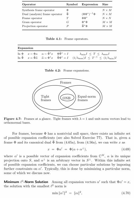
146 Chapter 4. Local Fourier and Wavelet Frames on Sequences
Operator Symbol Expression Size
Synthesis frame operator Φ N ×M
Dual (analysis) frame operator Φ (ΦΦ∗)−1Φ N ×M
Frame operator T ΦΦ∗ N ×N
Gram operator G Φ∗Φ M ×M
Projection operator P Φ∗Φ M ×M
Table 4.1: Frame operators.
Expansion
In Φ x = Φα α = Φ∗x ΦΦ∗ = I λminI ≤ T ≤ λmaxI
In Φ x = Φα α = Φ∗x ΦΦ∗ = I (1/λmax)I ≤ T−1 ≤ (1/λmin)I
Table 4.2: Frame expansions.
Frames
Tightframes
Equal-normframes
ONB
Figure 4.7: Frames at a glance. Tight frames with λ = 1 and unit-norm vectors lead toorthonormal bases.
For frames, because Φ has a nontrivial null space, there exists an infinite setof possible expansion coefficients (see also Solved Exercise ??). That is, given a
frame Φ and its canonical dual Φ from (4.65a), from (4.56a), we can write x as
x = Φα′ = Φ(α+ α⊥), (4.69)
where α′ is a possible vector of expansion coefficients from CM , α is its unique
projection onto S, and α⊥ is an arbitrary vector in S⊥. Within this infinite setof possible expansion coefficients, we can choose particular solutions by imposingfurther constraints on α′. Typically, this is done by minimizing a particular norm,some of which we discuss now.
Minimum ℓ2-Norm Solution Among all expansion vectors α′ such that Φα′ = x,the solution with the smallest ℓ2 norm is
min ‖α′‖2 = ‖α‖2, (4.70)
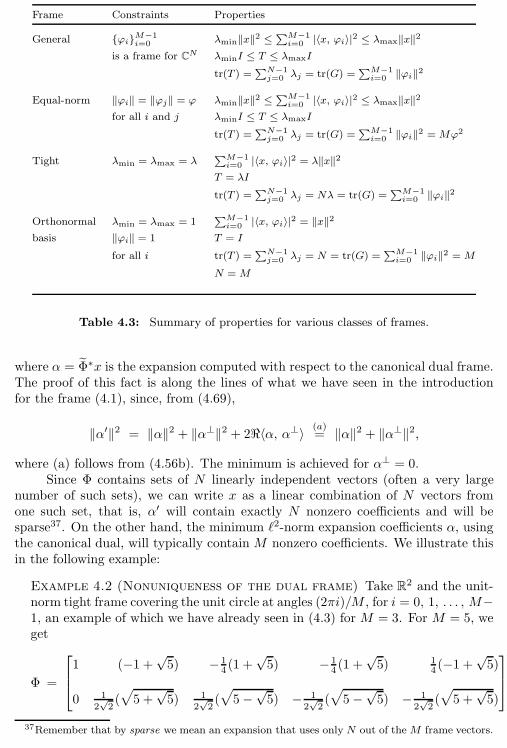
4.2. Finite-Dimensional Frames 147
Frame Constraints Properties
General ϕiM−1i=0 λmin‖x‖2 ≤
∑M−1i=0 |〈x, ϕi〉|2 ≤ λmax‖x‖2
is a frame for CN λminI ≤ T ≤ λmaxI
tr(T ) =∑N−1j=0 λj = tr(G) =
∑M−1i=0 ‖ϕi‖2
Equal-norm ‖ϕi‖ = ‖ϕj‖ = ϕ λmin‖x‖2 ≤∑M−1i=0 |〈x, ϕi〉|2 ≤ λmax‖x‖2
for all i and j λminI ≤ T ≤ λmaxI
tr(T ) =∑N−1j=0 λj = tr(G) =
∑M−1i=0 ‖ϕi‖2 =Mϕ2
Tight λmin = λmax = λ∑M−1i=0 |〈x, ϕi〉|2 = λ‖x‖2
T = λI
tr(T ) =∑N−1j=0 λj = Nλ = tr(G) =
∑M−1i=0 ‖ϕi‖2
Orthonormal λmin = λmax = 1∑M−1i=0 |〈x, ϕi〉|2 = ‖x‖2
basis ‖ϕi‖ = 1 T = I
for all i tr(T ) =∑N−1j=0 λj = N = tr(G) =
∑M−1i=0 ‖ϕi‖2 =M
N = M
Table 4.3: Summary of properties for various classes of frames.
where α = Φ∗x is the expansion computed with respect to the canonical dual frame.The proof of this fact is along the lines of what we have seen in the introductionfor the frame (4.1), since, from (4.69),
‖α′‖2 = ‖α‖2 + ‖α⊥‖2 + 2ℜ〈α, α⊥〉 (a)= ‖α‖2 + ‖α⊥‖2,
where (a) follows from (4.56b). The minimum is achieved for α⊥ = 0.Since Φ contains sets of N linearly independent vectors (often a very large
number of such sets), we can write x as a linear combination of N vectors fromone such set, that is, α′ will contain exactly N nonzero coefficients and will besparse37. On the other hand, the minimum ℓ2-norm expansion coefficients α, usingthe canonical dual, will typically contain M nonzero coefficients. We illustrate thisin the following example:
Example 4.2 (Nonuniqueness of the dual frame) Take R2 and the unit-norm tight frame covering the unit circle at angles (2πi)/M , for i = 0, 1, . . . , M−1, an example of which we have already seen in (4.3) for M = 3. For M = 5, weget
Φ =
1 (−1 +
√5) − 1
4 (1 +√5) − 1
4 (1 +√5) 1
4 (−1 +√5)
0 12√2(√5 +√5) 1
2√2(√5−√5) − 1
2√2(√5−√5) − 1
2√2(√5 +√5)
.
37Remember that by sparse we mean an expansion that uses only N out of theM frame vectors.
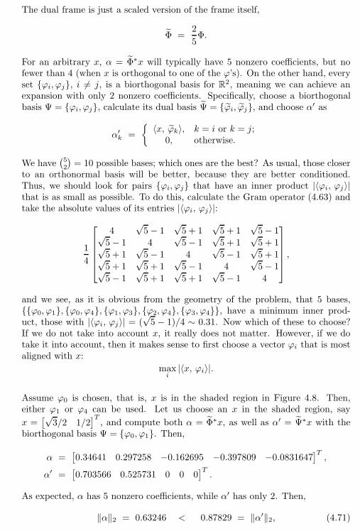
148 Chapter 4. Local Fourier and Wavelet Frames on Sequences
The dual frame is just a scaled version of the frame itself,
Φ =2
5Φ.
For an arbitrary x, α = Φ∗x will typically have 5 nonzero coefficients, but nofewer than 4 (when x is orthogonal to one of the ϕ’s). On the other hand, everyset ϕi, ϕj, i 6= j, is a biorthogonal basis for R2, meaning we can achieve anexpansion with only 2 nonzero coefficients. Specifically, choose a biorthogonalbasis Ψ = ϕi, ϕj, calculate its dual basis Ψ = ϕi, ϕj, and choose α′ as
α′k
=
〈x, ϕk〉, k = i or k = j;
0, otherwise.
We have(52
)= 10 possible bases; which ones are the best? As usual, those closer
to an orthonormal basis will be better, because they are better conditioned.Thus, we should look for pairs ϕi, ϕj that have an inner product |〈ϕi, ϕj〉|that is as small as possible. To do this, calculate the Gram operator (4.63) andtake the absolute values of its entries |〈ϕi, ϕj〉|:
1
4
4√5− 1
√5 + 1
√5 + 1
√5− 1√
5− 1 4√5− 1
√5 + 1
√5 + 1√
5 + 1√5− 1 4
√5− 1
√5 + 1√
5 + 1√5 + 1
√5− 1 4
√5− 1√
5− 1√5 + 1
√5 + 1
√5− 1 4
,
and we see, as it is obvious from the geometry of the problem, that 5 bases,ϕ0, ϕ1, ϕ0, ϕ4, ϕ1, ϕ3, ϕ2, ϕ4, ϕ3, ϕ4, have a minimum inner prod-uct, those with |〈ϕi, ϕj〉| = (
√5 − 1)/4 ∼ 0.31. Now which of these to choose?
If we do not take into account x, it really does not matter. However, if we dotake it into account, then it makes sense to first choose a vector ϕi that is mostaligned with x:
maxi
|〈x, ϕi〉|.
Assume ϕ0 is chosen, that is, x is in the shaded region in Figure 4.8. Then,either ϕ1 or ϕ4 can be used. Let us choose an x in the shaded region, say
x =[√
3/2 1/2]T
, and compute both α = Φ∗x, as well as α′ = Ψ∗x with thebiorthogonal basis Ψ = ϕ0, ϕ1. Then,
α =[0.34641 0.297258 −0.162695 −0.397809 −0.0831647
]T
,
α′ =[0.703566 0.525731 0 0 0
]T
.
As expected, α has 5 nonzero coefficients, while α′ has only 2. Then,
‖α‖2 = 0.63246 < 0.87829 = ‖α′‖2, (4.71)
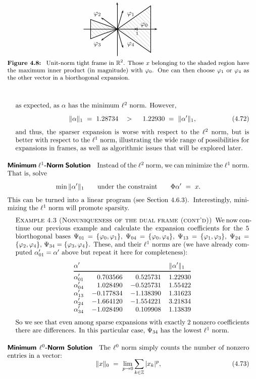
4.2. Finite-Dimensional Frames 149
1
ϕ0
ϕ1ϕ2
ϕ3 ϕ4
Figure 4.8: Unit-norm tight frame in R2. Those x belonging to the shaded region have
the maximum inner product (in magnitude) with ϕ0. One can then choose ϕ1 or ϕ4 asthe other vector in a biorthogonal expansion.
as expected, as α has the minimum ℓ2 norm. However,
‖α‖1 = 1.28734 > 1.22930 = ‖α′‖1, (4.72)
and thus, the sparser expansion is worse with respect to the ℓ2 norm, but isbetter with respect to the ℓ1 norm, illustrating the wide range of possibilities forexpansions in frames, as well as algorithmic issues that will be explored later.
Minimum ℓ1-Norm Solution Instead of the ℓ2 norm, we can minimize the ℓ1 norm.That is, solve
min ‖α′‖1 under the constraint Φα′ = x.
This can be turned into a linear program (see Section 4.6.3). Interestingly, mini-mizing the ℓ1 norm will promote sparsity.
Example 4.3 (Nonuniqueness of the dual frame (cont’d)) We now con-tinue our previous example and calculate the expansion coefficients for the 5biorthogonal bases Ψ01 = ϕ0, ϕ1, Ψ04 = ϕ0, ϕ4, Ψ13 = ϕ1, ϕ3, Ψ24 =ϕ2, ϕ4, Ψ34 = ϕ3, ϕ4. These, and their ℓ1 norms are (we have already com-puted α′
01 = α′ above but repeat it here for completeness):
α′ ‖α′‖1α′01 0.703566 0.525731 1.22930α′04 1.028490 −0.525731 1.55422α′13 −0.177834 −1.138390 1.31623α′24 −1.664120 −1.554221 3.21834α′34 −1.028490 0.109908 1.13839
So we see that even among sparse expansions with exactly 2 nonzero coefficientsthere are differences. In this particular case, Ψ34 has the lowest ℓ1 norm.
Minimum ℓ0-Norm Solution The ℓ0 norm simply counts the number of nonzeroentries in a vector:
‖x‖0 = limp→0
∑
k∈Z
|xk|p, (4.73)
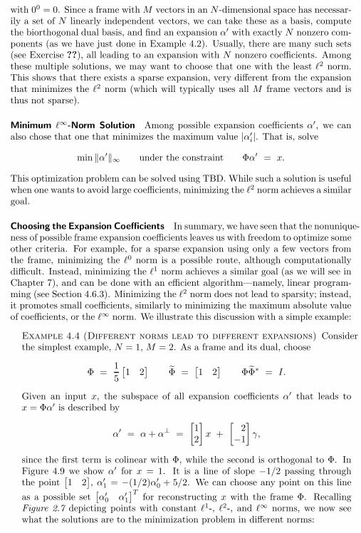
150 Chapter 4. Local Fourier and Wavelet Frames on Sequences
with 00 = 0. Since a frame withM vectors in an N -dimensional space has necessar-ily a set of N linearly independent vectors, we can take these as a basis, computethe biorthogonal dual basis, and find an expansion α′ with exactly N nonzero com-ponents (as we have just done in Example 4.2). Usually, there are many such sets(see Exercise ??), all leading to an expansion with N nonzero coefficients. Amongthese multiple solutions, we may want to choose that one with the least ℓ2 norm.This shows that there exists a sparse expansion, very different from the expansionthat minimizes the ℓ2 norm (which will typically uses all M frame vectors and isthus not sparse).
Minimum ℓ∞-Norm Solution Among possible expansion coefficients α′, we canalso chose that one that minimizes the maximum value |α′
i|. That is, solve
min ‖α′‖∞ under the constraint Φα′ = x.
This optimization problem can be solved using TBD. While such a solution is usefulwhen one wants to avoid large coefficients, minimizing the ℓ2 norm achieves a similargoal.
Choosing the Expansion Coefficients In summary, we have seen that the nonunique-ness of possible frame expansion coefficients leaves us with freedom to optimize someother criteria. For example, for a sparse expansion using only a few vectors fromthe frame, minimizing the ℓ0 norm is a possible route, although computationallydifficult. Instead, minimizing the ℓ1 norm achieves a similar goal (as we will see inChapter 7), and can be done with an efficient algorithm—namely, linear program-ming (see Section 4.6.3). Minimizing the ℓ2 norm does not lead to sparsity; instead,it promotes small coefficients, similarly to minimizing the maximum absolute valueof coefficients, or the ℓ∞ norm. We illustrate this discussion with a simple example:
Example 4.4 (Different norms lead to different expansions) Considerthe simplest example, N = 1, M = 2. As a frame and its dual, choose
Φ =1
5
[1 2
]Φ =
[1 2
]ΦΦ∗ = I.
Given an input x, the subspace of all expansion coefficients α′ that leads tox = Φα′ is described by
α′ = α+ α⊥ =
[12
]x +
[2−1
]γ,
since the first term is colinear with Φ, while the second is orthogonal to Φ. InFigure 4.9 we show α′ for x = 1. It is a line of slope −1/2 passing throughthe point
[1 2
], α′
1 = −(1/2)α′0 + 5/2. We can choose any point on this line
as a possible set[α′0 α′
1
]T
for reconstructing x with the frame Φ. RecallingFigure 2.7 depicting points with constant ℓ1-, ℓ2-, and ℓ∞ norms, we now seewhat the solutions are to the minimization problem in different norms:
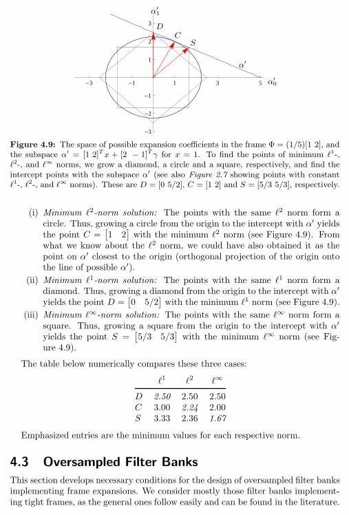
4.3. Oversampled Filter Banks 151
-3 -1 1 3 5
-3
-2
-1
1
2
3
α′0
α′1
α′
DC
S
Figure 4.9: The space of possible expansion coefficients in the frame Φ = (1/5)[1 2], andthe subspace α′ = [1 2]T x + [2 − 1]T γ for x = 1. To find the points of minimum ℓ1-,ℓ2-, and ℓ∞ norms, we grow a diamond, a circle and a square, respectively, and find theintercept points with the subspace α′ (see also Figure 2.7 showing points with constantℓ1-, ℓ2-, and ℓ∞ norms). These are D = [0 5/2], C = [1 2] and S = [5/3 5/3], respectively.
(i) Minimum ℓ2-norm solution: The points with the same ℓ2 norm form acircle. Thus, growing a circle from the origin to the intercept with α′ yieldsthe point C =
[1 2
]with the minimum ℓ2 norm (see Figure 4.9). From
what we know about the ℓ2 norm, we could have also obtained it as thepoint on α′ closest to the origin (orthogonal projection of the origin ontothe line of possible α′).
(ii) Minimum ℓ1-norm solution: The points with the same ℓ1 norm form adiamond. Thus, growing a diamond from the origin to the intercept with α′
yields the point D =[0 5/2
]with the minimum ℓ1 norm (see Figure 4.9).
(iii) Minimum ℓ∞-norm solution: The points with the same ℓ∞ norm form asquare. Thus, growing a square from the origin to the intercept with α′
yields the point S =[5/3 5/3
]with the minimum ℓ∞ norm (see Fig-
ure 4.9).
The table below numerically compares these three cases:
ℓ1 ℓ2 ℓ∞
D 2.50 2.50 2.50C 3.00 2.24 2.00S 3.33 2.36 1.67
Emphasized entries are the minimum values for each respective norm.
4.3 Oversampled Filter Banks
This section develops necessary conditions for the design of oversampled filter banksimplementing frame expansions. We consider mostly those filter banks implement-ing tight frames, as the general ones follow easily and can be found in the literature.
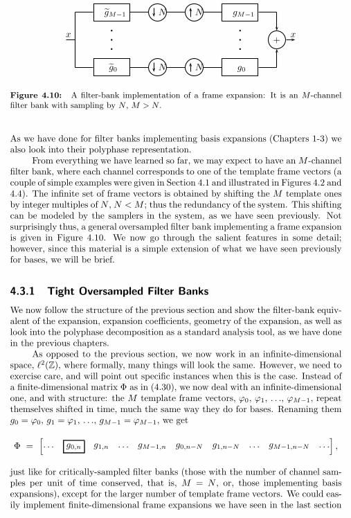
152 Chapter 4. Local Fourier and Wavelet Frames on Sequences
x
gM−1
g0
b
b
b
N
N
N
N
gM−1
g0
b
b
b
+x
Figure 4.10: A filter-bank implementation of a frame expansion: It is an M -channelfilter bank with sampling by N , M > N .
As we have done for filter banks implementing basis expansions (Chapters 1-3) wealso look into their polyphase representation.
From everything we have learned so far, we may expect to have anM -channelfilter bank, where each channel corresponds to one of the template frame vectors (acouple of simple examples were given in Section 4.1 and illustrated in Figures 4.2 and4.4). The infinite set of frame vectors is obtained by shifting the M template onesby integer multiples of N , N < M ; thus the redundancy of the system. This shiftingcan be modeled by the samplers in the system, as we have seen previously. Notsurprisingly thus, a general oversampled filter bank implementing a frame expansionis given in Figure 4.10. We now go through the salient features in some detail;however, since this material is a simple extension of what we have seen previouslyfor bases, we will be brief.
4.3.1 Tight Oversampled Filter Banks
We now follow the structure of the previous section and show the filter-bank equiv-alent of the expansion, expansion coefficients, geometry of the expansion, as well aslook into the polyphase decomposition as a standard analysis tool, as we have donein the previous chapters.
As opposed to the previous section, we now work in an infinite-dimensionalspace, ℓ2(Z), where formally, many things will look the same. However, we need toexercise care, and will point out specific instances when this is the case. Instead ofa finite-dimensional matrix Φ as in (4.30), we now deal with an infinite-dimensionalone, and with structure: the M template frame vectors, ϕ0, ϕ1, . . ., ϕM−1, repeatthemselves shifted in time, much the same way they do for bases. Renaming themg0 = ϕ0, g1 = ϕ1, . . ., gM−1 = ϕM−1, we get
Φ =[. . . g0,n g1,n . . . gM−1,n g0,n−N g1,n−N . . . gM−1,n−N . . .
],
just like for critically-sampled filter banks (those with the number of channel sam-ples per unit of time conserved, that is, M = N , or, those implementing basisexpansions), except for the larger number of template frame vectors. We could eas-ily implement finite-dimensional frame expansions we have seen in the last section
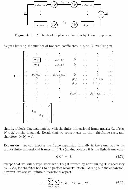
4.3. Oversampled Filter Banks 153
x
gM−1,−n
g0,−n
b
b
b
N
N
αM−1
α0
N
N
gM−1,n
g0,n
b
b
b
+x
Figure 4.11: A filter-bank implementation of a tight frame expansion.
by just limiting the number of nonzero coefficients in gi to N , resulting in
Φ =
. . ....
......
......
... . ..
. . . g0,0 . . . gM−1,0 0 . . . 0 . . .
. . . g0,1 . . . gM−1,1 0 . . . 0 . . .
. . ....
......
......
... . . .. . . g0,N−1 . . . gM−1,N−1 0 . . . 0 . . .. . . 0 . . . 0 g0,0 . . . gM−1,0 . . .. . . 0 . . . 0 g0,1 . . . gM−1,1 . . .
. . ....
......
......
... . . .. . . 0 . . . 0 g0,N−1 . . . gM−1,N−1 . . .
. .. ...
......
......
.... . .
=
. . ....
... . ..
. . . Φ0 . . .
. . . Φ0 . . .
. .. ...
.... . .
,
that is, a block-diagonal matrix, with the finite-dimensional frame matrix Φ0 of sizeN ×M on the diagonal. Recall that we concentrate on the tight-frame case, andtherefore, Φ0Φ
∗0 = I.
Expansion We can express the frame expansion formally in the same way as wedid for finite-dimensional frames in (4.32) (again, because it is the tight-frame case)
ΦΦ∗ = I, (4.74)
except that we will always work with 1-tight frames by normalizing Φ if necessaryby 1/
√λ, for the filter bank to be perfect reconstruction. Writing out the expansion,
however, we see its infinite-dimensional aspect:
x =
M−1∑
i=0
∑
k∈Z
〈x, gi,n−Nk〉 gi,n−Nk. (4.75)
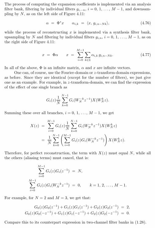
154 Chapter 4. Local Fourier and Wavelet Frames on Sequences
The process of computing the expansion coefficients is implemented via an analysisfilter bank, filtering by individual filters gi,−n, i = 0, 1, . . . , M − 1, and downsam-pling by N , as on the left side of Figure 4.11:
α = Φ∗x αi,k = 〈x, gi,n−Nk〉, (4.76)
while the process of reconstructing x is implemented via a synthesis filter bank,upsampling by N and filtering by individual filters gi,n, i = 0, 1, . . . , M − 1, as onthe right side of Figure 4.11:
x = Φα x =
M−1∑
i=0
∑
k∈Z
αi,k gi,n−Nk. (4.77)
In all of the above, Φ is an infinite matrix, α and x are infinite vectors.One can, of course, use the Fourier-domain or z-transform-domain expressions,
as before. Since they are identical (except for the number of filters), we just giveone as an example. For example, in z-transform-domain, we can find the expressionof the effect of one single branch as
Gi(z)1
N
N−1∑
k=0
Gi(W−kNz−1)X(W k
Nz).
Summing these over all branches, i = 0, 1, . . . , M − 1, we get
X(z) =
M−1∑
i=0
Gi(z)1
N
N−1∑
k=0
Gi(W−kNz−1)X(W k
Nz)
=1
N
N−1∑
k=0
(M−1∑
i=0
Gi(z)Gi(W−kNz−1)
)X(W k
Nz).
Therefore, for perfect reconstruction, the term with X(z) must equal N , while allthe others (aliasing terms) must cancel, that is:
M−1∑
i=0
Gi(z)Gi(z−1) = N,
M−1∑
i=0
Gi(z)Gi(W−kNz−1) = 0, k = 1, 2, . . . , M − 1.
For example, for N = 2 and M = 3, we get that:
G0(z)G0(z−1) +G1(z)G1(z
−1) +G2(z)G2(z−1) = 2,
G0(z)G0(−z−1) +G1(z)G1(−z−1) +G2(z)G2(−z−1) = 0.
Compare this to its counterpart expression in two-channel filter banks in (1.28).
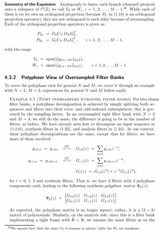
4.3. Oversampled Filter Banks 155
Geometry of the Expansion Analogously to bases, each branch (channel) projectsonto a subspace of ℓ2(Z) we call V0 or Wi, i = 1, 2, . . . , M − 1.38 While each ofthese is on its own an orthogonal projection (because PV in (1.18) is an orthogonalprojection operator), they are not orthogonal to each other because of oversampling.Each of the orthogonal projection operators is given as
PV0 = G0UN DNGT
0 ,
PWi= GiUN DNG
T
i, i = 1, 2, . . . , M − 1,
with the range
V0 = span(g0,n−Nkk∈Z),
Wi = span(gi,n−Nkk∈Z), i = 1, 2, . . . ,M − 1.
4.3.2 Polyphase View of Oversampled Filter Banks
To cover the polyphase view for general N and M , we cover it through an examplewith N = 2, M = 3; expressions for general N and M follow easily.
Example 4.5 (Tight oversampled 3-channel filter banks) For two-channelfilter banks, a polyphase decomposition is achieved by simply splitting both se-quences and filters into their even- and odd-indexed subsequences; this is gov-erned by the sampling factor. In an oversampled tight filter bank with N = 2and M = 3, we still do the same; the difference is going to be in the number offilters, as before. We have already seen how to decompose an input sequence in(3.216), synthesis filters in (1.32), and analysis filters in (1.34). In our context,these polyphase decompositions are the same, except that for filters, we havemore of them involved:
gi,0,n = gi,2nZT←→ Gi,0(z) =
∑
n∈Z
gi,2nz−n,
gi,1,n = gi,2n+1ZT←→ Gi,1(z) =
∑
n∈Z
gi,2n+1z−n,
Gi(z) = Gi,0(z2) + z−1Gi,1(z
2),
for i = 0, 1, 2 and synthesis filters. That is, we have 3 filters with 2 polyphasecomponents each, leading to the following synthesis polyphase matrix Φp(z):
Φp(z) =
[G0,0(z) G1,0(z) G2,0(z)G0,1(z) G1,1(z) G2,1(z)
].
As expected, the polyphase matrix is no longer square; rather, it is a (2 × 3)matrix of polynomials. Similarly, on the analysis side, since this is a filter bankimplementing a tight frame with Φ = Φ, we assume the same filters as on the
38We assume here that the space V0 is lowpass in nature, while the Wi are bandpass.
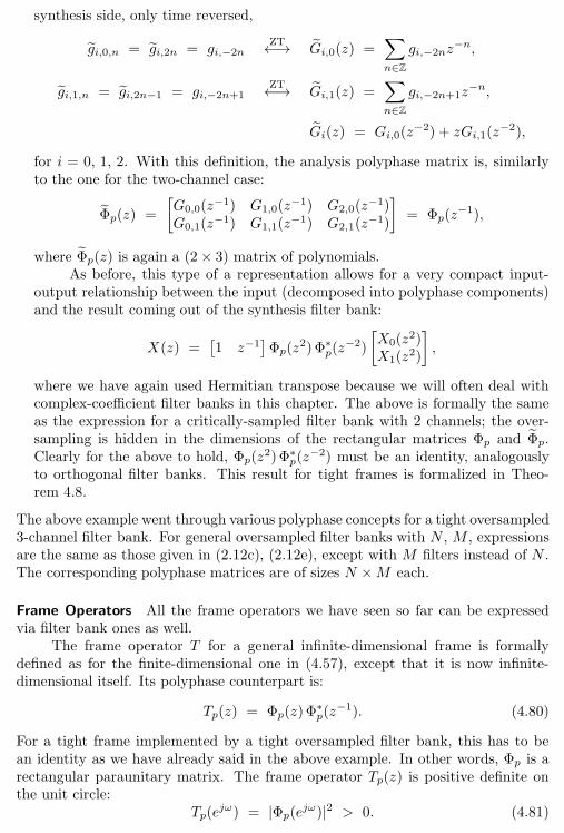
156 Chapter 4. Local Fourier and Wavelet Frames on Sequences
synthesis side, only time reversed,
gi,0,n = gi,2n = gi,−2nZT←→ Gi,0(z) =
∑
n∈Z
gi,−2nz−n,
gi,1,n = gi,2n−1 = gi,−2n+1ZT←→ Gi,1(z) =
∑
n∈Z
gi,−2n+1z−n,
Gi(z) = Gi,0(z−2) + zGi,1(z
−2),
for i = 0, 1, 2. With this definition, the analysis polyphase matrix is, similarlyto the one for the two-channel case:
Φp(z) =
[G0,0(z
−1) G1,0(z−1) G2,0(z
−1)G0,1(z
−1) G1,1(z−1) G2,1(z
−1)
]= Φp(z
−1),
where Φp(z) is again a (2× 3) matrix of polynomials.As before, this type of a representation allows for a very compact input-
output relationship between the input (decomposed into polyphase components)and the result coming out of the synthesis filter bank:
X(z) =[1 z−1
]Φp(z
2)Φ∗p(z−2)
[X0(z
2)X1(z
2)
],
where we have again used Hermitian transpose because we will often deal withcomplex-coefficient filter banks in this chapter. The above is formally the sameas the expression for a critically-sampled filter bank with 2 channels; the over-sampling is hidden in the dimensions of the rectangular matrices Φp and Φp.Clearly for the above to hold, Φp(z
2)Φ∗p(z−2) must be an identity, analogously
to orthogonal filter banks. This result for tight frames is formalized in Theo-rem 4.8.
The above example went through various polyphase concepts for a tight oversampled3-channel filter bank. For general oversampled filter banks with N , M , expressionsare the same as those given in (2.12c), (2.12e), except with M filters instead of N .The corresponding polyphase matrices are of sizes N ×M each.
Frame Operators All the frame operators we have seen so far can be expressedvia filter bank ones as well.
The frame operator T for a general infinite-dimensional frame is formallydefined as for the finite-dimensional one in (4.57), except that it is now infinite-dimensional itself. Its polyphase counterpart is:
Tp(z) = Φp(z)Φ∗p(z−1). (4.80)
For a tight frame implemented by a tight oversampled filter bank, this has to bean identity as we have already said in the above example. In other words, Φp is arectangular paraunitary matrix. The frame operator Tp(z) is positive definite onthe unit circle:
Tp(ejω) = |Φp(ejω)|2 > 0. (4.81)
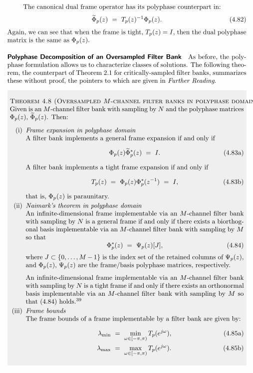
4.3. Oversampled Filter Banks 157
The canonical dual frame operator has its polyphase counterpart in:
Φp(z) = Tp(z)−1Φp(z). (4.82)
Again, we can see that when the frame is tight, Tp(z) = I, then the dual polyphasematrix is the same as Φp(z).
Polyphase Decomposition of an Oversampled Filter Bank As before, the poly-phase formulation allows us to characterize classes of solutions. The following theo-rem, the counterpart of Theorem 2.1 for critically-sampled filter banks, summarizesthese without proof, the pointers to which are given in Further Reading.
Theorem 4.8 (Oversampled M -channel filter banks in polyphase domain)Given is anM -channel filter bank with sampling by N and the polyphase matricesΦp(z), Φp(z). Then:
(i) Frame expansion in polyphase domainA filter bank implements a general frame expansion if and only if
Φp(z)Φ∗p(z) = I. (4.83a)
A filter bank implements a tight frame expansion if and only if
Tp(z) = Φp(z)Φ∗p(z−1) = I, (4.83b)
that is, Φp(z) is paraunitary.
(ii) Naimark’s theorem in polyphase domainAn infinite-dimensional frame implementable via an M -channel filter bankwith sampling by N is a general frame if and only if there exists a biorthog-onal basis implementable via an M -channel filter bank with sampling by Mso that
Φ∗p(z) = Ψp(z)[J ], (4.84)
where J ⊂ 0, . . . ,M − 1 is the index set of the retained columns of Ψp(z),and Φp(z), Ψp(z) are the frame/basis polyphase matrices, respectively.
An infinite-dimensional frame implementable via an M -channel filter bankwith sampling by N is a tight frame if and only if there exists an orthonormalbasis implementable via an M -channel filter bank with sampling by M sothat (4.84) holds.39
(iii) Frame boundsThe frame bounds of a frame implementable by a filter bank are given by:
λmin = minω∈[−π,π)
Tp(ejω), (4.85a)
λmax = maxω∈[−π,π)
Tp(ejω). (4.85b)

158 Chapter 4. Local Fourier and Wavelet Frames on Sequences
The last statement on eigenvalues stems from the fact that the frame operatorT and its polyphase counterpart Tp(e
jω) are related via a unitary transformation.If the eigenvalues of Tp(e
jω) are defined via Tp(ejω)v(ω) = λ(ω)v(ω), then the
eigenvalues of T and Tp(ejω) are the same, leading to (4.85).
Example 4.6 (Tight oversampled 3-channel filter banks cont’d) Wenow set M = 3, N = 2 and show how one can obtain a linear-phase tight framewith filters of length greater than 2, a solution not possible for critically-sampledfilter banks with sampling by 2, as was shown in Theorem 1.12. We know thatsuch a filter bank implementing a tight frame transform must be seeded from anorthogonal filter bank with a 3× 3 paraunitary matrix.
We use such a matrix in the example showing how to parameterize N -channel orthogonal filter banks, Example 2.2 with K = 2, that is, all polyphasecomponents will be first-degree polynomials in z−1. We form a tight frame bydeleting its last column and call the resulting frame polyphase matrix ΦT
p(z).
Since there are 5 angles involved, the matrix is too big to explicitly state here;instead, we start imposing the linear-phase conditions to reduce the number ofdegrees of freedom. A simple solution with θ00 = π/2, θ11 = π/2, θ02 = π/4 andθ10 = 3π/4, leads to the first two filters being symmetric of length 3 and the lastantisymmetric of length 3. The resulting polyphase matrix is (where we haverescaled the first and third columns by −1):
Φp(z) =
[12 cos θ01(1 + z−1) 1
2 sin θ01(1 + z−1) 12 (1 − z−1)
sin θ01 − cos θ01 0
]T
,
leading to the following three filters:
G0(z) =1
2cos θ01 + sin θ01z
−1 +1
2cos θ01z
−2,
G1(z) =1
2sin θ01 − cos θ01z
−1 +1
2sin θ01z
−2,
G2(z) =1
2− 1
2z−2.
For example, with θ01 = π/3, the three resulting filters have reasonable coverageof the frequency axis (see Figure 4.12).
4.4 Local Fourier Frames
Until now, the material in this chapter covered finite-dimensional frames (Sec-tion 4.2) and oversampled filter banks as a vehicle for implementing both finite-dimensional as well as certain infinite-dimensional frames (previous section). Wenow investigate a more specific class of frames; those obtained by modulating (shift-ing in frequency) a single prototype filter/frame vector, introduced in their basisform in Chapter 2. These are some of the oldest bases and frames, and some of themost widely used. The local Fourier expansions arose in response to the need to
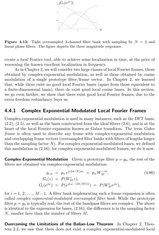
4.4. Local Fourier Frames 159
0Π
2Π
0.5
1.
1.5
ω
|Gi(ejω)|
Figure 4.12: Tight oversampled 3-channel filter bank with sampling by N = 2 andlinear-phase filters. The figure depicts the three magnitude responses.
create a local Fourier tool, able to achieve some localization in time, at the price ofworsening the known excellent localization in frequency.
As in Chapter 2, we will consider two large classes of local Fourier frames, thoseobtained by complex-exponential modulation, as well as those obtained by cosinemodulation of a single prototype filter/frame vector. In Chapter 2, we learnedthat, while there exist no good local Fourier bases (apart from those equivalent toa finite-dimensional basis), there do exist good local cosine bases. In this section,we go even farther; we show that there exist good local Fourier frames, due to theextra freedom redundancy buys us.
4.4.1 Complex Exponential-Modulated Local Fourier Frames
Complex-exponential modulation is used in many instances, such as the DFT basis,(2.2), (2.5), as well as the basis constructed from the ideal filters (2.6), and is at theheart of the local Fourier expansion known as Gabor transform. The term Gaborframe is often used to describe any frame with complex-exponential modulationand overlapping frame vectors (oversampled filter banks with filters of lengths longerthan the sampling factor N). For complex exponential-modulated bases, we definedthis modulation in (2.16); for complex exponential-modulated frames, we do it now.
Complex-Exponential Modulation Given a prototype filter p = g0, the rest of thefilters are obtained via complex-exponential modulation:
gi,n = pn ej(2π/N)in = pnW
−inM
, (4.86)
Gi(z) = P (W i
Mz),
Gi(ejω) = P (ej(ω−(2π/M)i)) = P (W i
Mejω),
for i = 1, 2, . . . , M −1. A filter bank implementing such a frame expansion is oftencalled complex exponential-modulated oversampled filter bank. While the prototypefilter p = g0 is typically real, the rest of the bandpass filters are complex. The aboveis identical to the expression for bases, (2.16); the difference is in the sampling factorN , smaller here than the number of filters M .
Overcoming the Limitations of the Balian-Low Theorem In Chapter 2, Theo-rem 2.2, we saw that there does not exist a complex exponential-modulated local
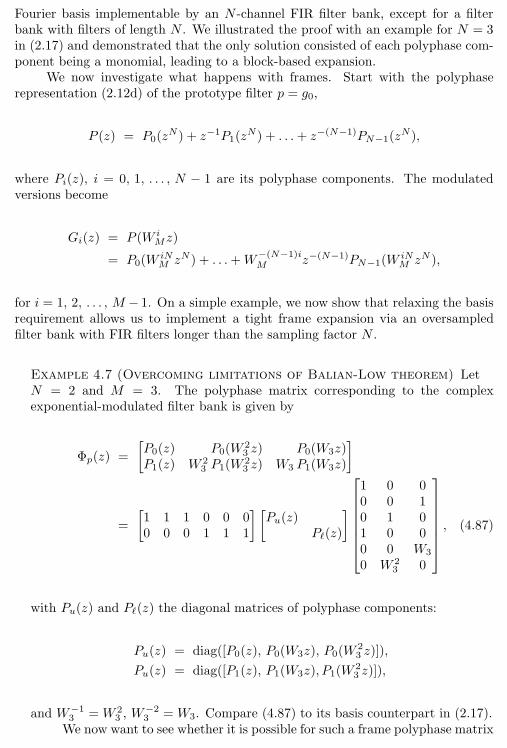
160 Chapter 4. Local Fourier and Wavelet Frames on Sequences
Fourier basis implementable by an N -channel FIR filter bank, except for a filterbank with filters of length N . We illustrated the proof with an example for N = 3in (2.17) and demonstrated that the only solution consisted of each polyphase com-ponent being a monomial, leading to a block-based expansion.
We now investigate what happens with frames. Start with the polyphaserepresentation (2.12d) of the prototype filter p = g0,
P (z) = P0(zN) + z−1P1(z
N) + . . .+ z−(N−1)PN−1(zN),
where Pi(z), i = 0, 1, . . . , N − 1 are its polyphase components. The modulatedversions become
Gi(z) = P (W i
Mz)
= P0(WiN
MzN) + . . .+W
−(N−1)iM
z−(N−1)PN−1(WiN
MzN ),
for i = 1, 2, . . . , M − 1. On a simple example, we now show that relaxing the basisrequirement allows us to implement a tight frame expansion via an oversampledfilter bank with FIR filters longer than the sampling factor N .
Example 4.7 (Overcoming limitations of Balian-Low theorem) LetN = 2 and M = 3. The polyphase matrix corresponding to the complexexponential-modulated filter bank is given by
Φp(z) =
[P0(z) P0(W
23 z) P0(W3z)
P1(z) W 23 P1(W
23 z) W3 P1(W3z)
]
=
[1 1 1 0 0 00 0 0 1 1 1
] [Pu(z)
Pℓ(z)
]
1 0 00 0 10 1 01 0 00 0 W3
0 W 23 0
, (4.87)
with Pu(z) and Pℓ(z) the diagonal matrices of polyphase components:
Pu(z) = diag([P0(z), P0(W3z), P0(W23 z)]),
Pu(z) = diag([P1(z), P1(W3z), P1(W23 z)]),
and W−13 =W 2
3 , W−23 =W3. Compare (4.87) to its basis counterpart in (2.17).
We now want to see whether it is possible for such a frame polyphase matrix
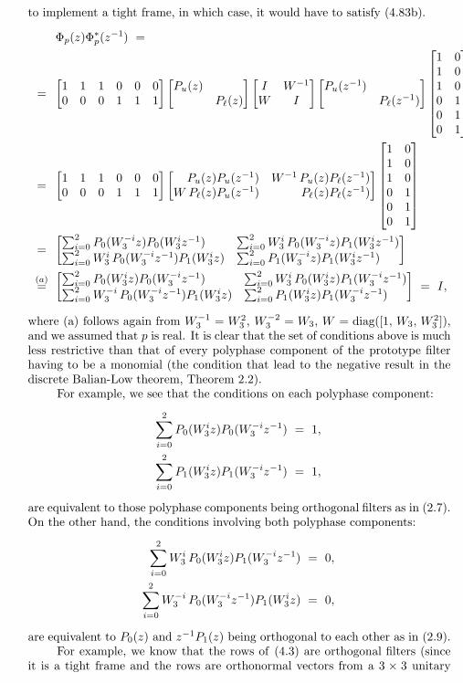
4.4. Local Fourier Frames 161
to implement a tight frame, in which case, it would have to satisfy (4.83b).
Φp(z)Φ∗p(z−1) =
=
[1 1 1 0 0 00 0 0 1 1 1
] [Pu(z)
Pℓ(z)
] [I W−1
W I
] [Pu(z
−1)Pℓ(z
−1)
]
1 01 01 00 10 10 1
=
[1 1 1 0 0 00 0 0 1 1 1
] [Pu(z)Pu(z
−1) W−1 Pu(z)Pℓ(z−1)
W Pℓ(z)Pu(z−1) Pℓ(z)Pℓ(z
−1)
]
1 01 01 00 10 10 1
=
[∑2i=0 P0(W
−i3 z)P0(W
i
3z−1)
∑2i=0W
i
3 P0(W−i3 z)P1(W
i
3z−1)∑2
i=0Wi
3 P0(W−i3 z−1)P1(W
i
3z)∑2
i=0 P1(W−i3 z)P1(W
i
3z−1)
]
(a)=
[∑2i=0 P0(W
i
3z)P0(W−i3 z−1)
∑2i=0W
i
3 P0(Wi
3z)P1(W−i3 z−1)∑2
i=0W−i3 P0(W
−i3 z−1)P1(W
i
3z)∑2
i=0 P1(Wi
3z)P1(W−i3 z−1)
]= I,
where (a) follows again from W−13 = W 2
3 , W−23 = W3, W = diag([1, W3, W
23 ]),
and we assumed that p is real. It is clear that the set of conditions above is muchless restrictive than that of every polyphase component of the prototype filterhaving to be a monomial (the condition that lead to the negative result in thediscrete Balian-Low theorem, Theorem 2.2).
For example, we see that the conditions on each polyphase component:
2∑
i=0
P0(Wi
3z)P0(W−i3 z−1) = 1,
2∑
i=0
P1(Wi
3z)P1(W−i3 z−1) = 1,
are equivalent to those polyphase components being orthogonal filters as in (2.7).On the other hand, the conditions involving both polyphase components:
2∑
i=0
W i
3 P0(Wi
3z)P1(W−i3 z−1) = 0,
2∑
i=0
W−i3 P0(W
−i3 z−1)P1(W
i
3z) = 0,
are equivalent to P0(z) and z−1P1(z) being orthogonal to each other as in (2.9).
For example, we know that the rows of (4.3) are orthogonal filters (sinceit is a tight frame and the rows are orthonormal vectors from a 3 × 3 unitary
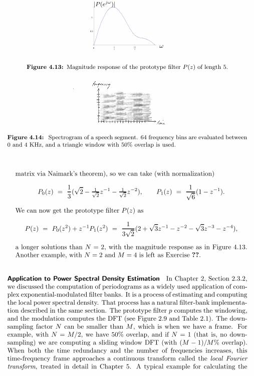
162 Chapter 4. Local Fourier and Wavelet Frames on Sequences
0Π
3
2Π
3
0.5
1.
ω
|P (ejω)|
Figure 4.13: Magnitude response of the prototype filter P (z) of length 5.
Figure 4.14: Spectrogram of a speech segment. 64 frequency bins are evaluated between0 and 4 KHz, and a triangle window with 50% overlap is used.
matrix via Naimark’s theorem), so we can take (with normalization)
P0(z) =1
3(√2− 1√
2z−1 − 1√
2z−2), P1(z) =
1√6(1− z−1).
We can now get the prototype filter P (z) as
P (z) = P0(z2) + z−1P1(z
2) =1
3√2(2 +
√3z−1 − z−2 −
√3z−3 − z−4),
a longer solutions than N = 2, with the magnitude response as in Figure 4.13.Another example, with N = 2 and M = 4 is left as Exercise ??.
Application to Power Spectral Density Estimation In Chapter 2, Section 2.3.2,we discussed the computation of periodograms as a widely used application of com-plex exponential-modulated filter banks. It is a process of estimating and computingthe local power spectral density. That process has a natural filter-bank implementa-tion described in the same section. The prototype filter p computes the windowing,and the modulation computes the DFT (see Figure 2.9 and Table 2.1). The down-sampling factor N can be smaller than M , which is when we have a frame. Forexample, with N = M/2, we have 50% overlap, and if N = 1 (that is, no down-sampling) we are computing a sliding window DFT (with (M − 1)/M% overlap).When both the time redundancy and the number of frequencies increases, thistime-frequency frame approaches a continuous transform called the local Fouriertransform, treated in detail in Chapter 5. A typical example for calculating the
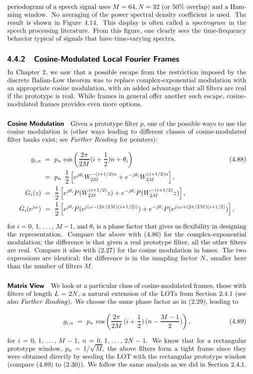
4.4. Local Fourier Frames 163
periodogram of a speech signal uses M = 64, N = 32 (or 50% overlap) and a Ham-ming window. No averaging of the power spectral density coefficient is used. Theresult is shown in Figure 4.14. This display is often called a spectrogram in thespeech processing literature. From this figure, one clearly sees the time-frequencybehavior typical of signals that have time-varying spectra.
4.4.2 Cosine-Modulated Local Fourier Frames
In Chapter 2, we saw that a possible escape from the restriction imposed by thediscrete Balian-Low theorem was to replace complex-exponential modulation withan appropriate cosine modulation, with an added advantage that all filters are realif the prototype is real. While frames in general offer another such escape, cosine-modulated frames provides even more options.
Cosine Modulation Given a prototype filter p, one of the possible ways to use thecosine modulation is (other ways leading to different classes of cosine-modulatedfilter banks exist; see Further Reading for pointers):
gi,n = pn cos
(2π
2M(i +
1
2)n+ θi
)(4.88)
= pn1
2
[ejθiW
−(i+1/2)n2M + e−jθiW (i+1/2)n
2M
],
Gi(z) =1
2
[ejθiP (W
(i+1/2)2M z) + e−jθiP (W−(i+1/2)
2M z)],
Gi(ejω) =
1
2
[ejθiP (ej(ω−(2π/2M)(i+1/2))) + e−jθiP (ej(ω+(2π/2M)(i+1/2))
],
for i = 0, 1, . . . , M −1, and θi is a phase factor that gives us flexibility in designingthe representation. Compare the above with (4.86) for the complex-exponentialmodulation; the difference is that given a real prototype filter, all the other filtersare real. Compare it also with (2.27) for the cosine modulation in bases. The twoexpressions are identical; the difference is in the sampling factor N , smaller herethan the number of filters M .
Matrix View We look at a particular class of cosine-modulated frames, those withfilters of length L = 2N , a natural extension of the LOTs from Section 2.4.1 (seealso Further Reading). We choose the same phase factor as in (2.29), leading to
gi,n = pn cos
(2π
2M(i+
1
2) (n− M − 1
2)
), (4.89)
for i = 0, 1, . . . , M − 1, n = 0, 1, . . . , 2N − 1. We know that for a rectangularprototype window, pn = 1/
√M , the above filters form a tight frame since they
were obtained directly by seeding the LOT with the rectangular prototype window(compare (4.89) to (2.30)). We follow the same analysis as we did in Section 2.4.1.
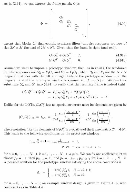
164 Chapter 4. Local Fourier and Wavelet Frames on Sequences
As in (2.34), we can express the frame matrix Φ as
Φ =
. . .
G0
G1 G0
G1 G0
G1
. . .
, (4.90)
except that blocks Gi that contain synthesis filters’ impulse responses are now ofsize 2N ×M (instead of 2N ×N). Given that the frame is tight (and real),
G0GT
0 +G1GT
1 = I, (4.91a)
G1GT
0 = G0GT
1 = 0. (4.91b)
Assume we want to impose a prototype window; then, as in (2.41), the windowedimpulse responses are G′
0 = P0G0 and G′1 = P1G1, where P0 and P1 are the N ×N
diagonal matrices with the left and right tails of the prototype window p on thediagonal, and if the prototype window is symmetric, P1 = JP0J . We can thussubstitute G′
0 and G′1 into (4.91) to verify that the resulting frame is indeed tight
G′0G
′T0 +G′
1G′T1 = P0G0G
T
0 P0 + P1G1GT
1 P1
= P0G0GT
0 P0 + JP0JG1GT
1 JP0J = I.
Unlike for the LOTs, G0GT
0 has no special structure now; its elements are given by
(G0GT
0 )i,n = ti,n =1
2M
sin(π(i+n+1)
2
)
sin(π(i+n+1)
2M
) +1
2M
sin(π(i−n)
2
)
sin(π(i−n)2M
) ,
where notation t for the elements ofG0GT
0 is evocative of the frame matrix T = ΦΦ∗.This leads to the following conditions on the prototype window:
tn,n p2n+ (1− tn,n) p2N−n−1 = 1,
pn pk = pN−n−1 pN−k−1,
for n = 0, 1, . . . , N−1, k = 0, 1, . . . , N−1, k 6= n. We can fix one coefficient; let uschoose p0 = −1, then pN−1 = ±1 and pk = −pN−1 pN−k−1 for k = 1, 2, . . . , N − 2.A possible solution for the prototype window satisfying the above conditions is
dn =
− cos( nπ
N−1), N = 2k + 1;
− cos( 2nπN−1), N = 2k,
for n = 0, 1, . . . , N − 1; an example window design is given in Figure 4.15, withcoefficients as in Table 4.4.
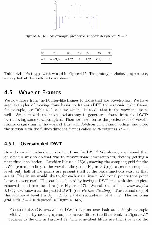
4.5. Wavelet Frames 165
2 4 6 8 10 12
-1.0
-0.5
0.5
1.0
n
pn
Figure 4.15: An example prototype window design for N = 7.
p0 p1 p2 p3 p4 p5 p6
−1 −√3/2 −1/2 0 1/2
√3/2 1
Table 4.4: Prototype window used in Figure 4.15. The prototype window is symmetric,so only half of the coefficients are shown.
4.5 Wavelet Frames
We now move from the Fourier-like frames to those that are wavelet-like. We haveseen examples of moving from bases to frames (DFT to harmonic tight frame,for example, see Table 4.7), and we would like to do that in the wavelet case aswell. We start with the most obvious way to generate a frame from the DWT:by removing some downsamplers. Then we move on to the predecessor of waveletframes originating in the work of Burt and Adelson on pyramid coding, and closethe section with the fully-redundant frames called shift-invariant DWT.
4.5.1 Oversampled DWT
How do we add redundancy starting from the DWT? We already mentioned thatan obvious way to do that was to remove some downsamplers, thereby getting afiner time localization. Consider Figure 4.16(a), showing the sampling grid for theDWT (corresponding to the wavelet tiling from Figure 3.7(d)): at each subsequentlevel, only half of the points are present (half of the basis functions exist at thatscale). Ideally, we would like to, for each scale, insert additional points (one pointbetween every two). This can be achieved by having a DWT tree with the samplersremoved at all free branches (see Figure 4.17). We call this scheme oversampledDWT, also known as the partial DWT (see Further Reading). The redundancy ofthis scheme at level ℓ is Aj = 2, for a total redundancy of A = 2. The samplinggrid with J = 4 is depicted in Figure 4.16(b).
Example 4.8 (Oversampled DWT) Let us now look at a simple examplewith J = 3. By moving upsamplers across filters, the filter bank in Figure 4.17reduces to the one in Figure 4.18. The equivalent filters are then (we leave the
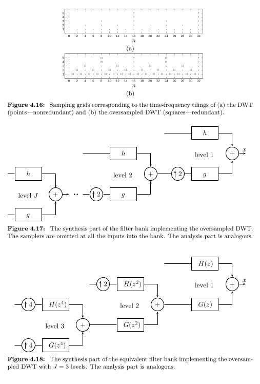
166 Chapter 4. Local Fourier and Wavelet Frames on Sequences
0 2 4 6 8 10 12 14 16 18 20 22 24 26 28 30 32
12345
n
(a)
0 2 4 6 8 10 12 14 16 18 20 22 24 26 28 30 32
12345
n
(b)
Figure 4.16: Sampling grids corresponding to the time-frequency tilings of (a) the DWT(points—nonredundant) and (b) the oversampled DWT (squares—redundant).
h
g
level J + b b 2
h
g
level 2 + 2
h
g
level 1 +x
Figure 4.17: The synthesis part of the filter bank implementing the oversampled DWT.The samplers are omitted at all the inputs into the bank. The analysis part is analogous.
4
4 H(z4)
G(z4)
level 3 +
2 H(z2)
G(z2)
level 2 +
H(z)
G(z)
level 1 +x
Figure 4.18: The synthesis part of the equivalent filter bank implementing the oversam-pled DWT with J = 3 levels. The analysis part is analogous.
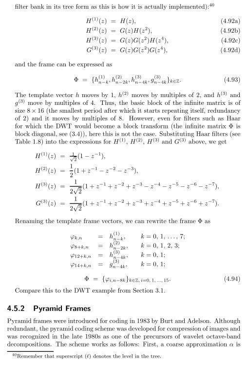
4.5. Wavelet Frames 167
filter bank in its tree form as this is how it is actually implemented):40
H(1)(z) = H(z), (4.92a)
H(2)(z) = G(z)H(z2), (4.92b)
H(3)(z) = G(z)G(z2)H(z4), (4.92c)
G(3)(z) = G(z)G(z2)G(z4), (4.92d)
and the frame can be expressed as
Φ = h(1)n−k, h
(2)n−2k, h
(3)n−4k, g
(3)n−4kk∈Z. (4.93)
The template vector h moves by 1, h(2) moves by multiples of 2, and h(3) andg(3) move by multiples of 4. Thus, the basic block of the infinite matrix is ofsize 8× 16 (the smallest period after which it starts repeating itself, redundancyof 2) and it moves by multiples of 8. However, even for filters such as Haarfor which the DWT would become a block transform (the infinite matrix Φ isblock diagonal, see (3.4)), here this is not the case. Substituting Haar filters (seeTable 1.8) into the expressions for H(1), H(2), H(3) and G(3) above, we get
H(1)(z) = 1√2(1− z−1),
H(2)(z) =1
2(1 + z−1 − z−2 − z−3),
H(3)(z) =1
2√2(1 + z−1 + z−2 + z−3 − z−4 − z−5 − z−6 − z−7),
G(3)(z) =1
2√2(1 + z−1 + z−2 + z−3 + z−4 + z−5 + z−6 + z−7).
Renaming the template frame vectors, we can rewrite the frame Φ as
ϕk,n = h(1)n−k, k = 0, 1, . . . , 7;
ϕ8+k,n = h(2)n−2k, k = 0, 1, 2, 3;
ϕ12+k,n = h(3)n−4k, k = 0, 1;
ϕ14+k,n = g(3)n−4k, k = 0, 1;
Φ = ϕi,n−8kk∈Z, i=0, 1, ..., 15. (4.94)
Compare this to the DWT example from Section 3.1.
4.5.2 Pyramid Frames
Pyramid frames were introduced for coding in 1983 by Burt and Adelson. Althoughredundant, the pyramid coding scheme was developed for compression of images andwas recognized in the late 1980s as one of the precursors of wavelet octave-banddecompositions. The scheme works as follows: First, a coarse approximation α is
40Remember that superscript (ℓ) denotes the level in the tree.
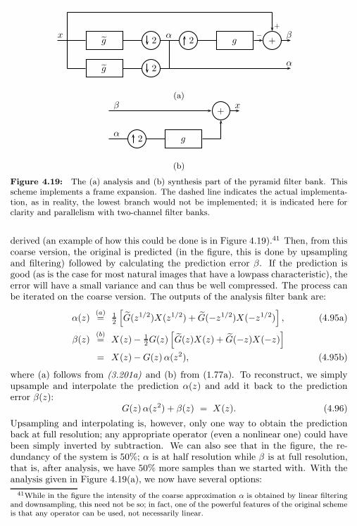
168 Chapter 4. Local Fourier and Wavelet Frames on Sequences
xg
g
2
2
α2 g
+
−+
β
α
(a)β
α2 g
+x
(b)
Figure 4.19: The (a) analysis and (b) synthesis part of the pyramid filter bank. Thisscheme implements a frame expansion. The dashed line indicates the actual implementa-tion, as in reality, the lowest branch would not be implemented; it is indicated here forclarity and parallelism with two-channel filter banks.
derived (an example of how this could be done is in Figure 4.19).41 Then, from thiscoarse version, the original is predicted (in the figure, this is done by upsamplingand filtering) followed by calculating the prediction error β. If the prediction isgood (as is the case for most natural images that have a lowpass characteristic), theerror will have a small variance and can thus be well compressed. The process canbe iterated on the coarse version. The outputs of the analysis filter bank are:
α(z)(a)= 1
2
[G(z1/2)X(z1/2) + G(−z1/2)X(−z1/2)
], (4.95a)
β(z)(b)= X(z)− 1
2G(z)[G(z)X(z) + G(−z)X(−z)
]
= X(z)−G(z)α(z2), (4.95b)
where (a) follows from (3.201a) and (b) from (1.77a). To reconstruct, we simplyupsample and interpolate the prediction α(z) and add it back to the predictionerror β(z):
G(z)α(z2) + β(z) = X(z). (4.96)
Upsampling and interpolating is, however, only one way to obtain the predictionback at full resolution; any appropriate operator (even a nonlinear one) could havebeen simply inverted by subtraction. We can also see that in the figure, the re-dundancy of the system is 50%; α is at half resolution while β is at full resolution,that is, after analysis, we have 50% more samples than we started with. With theanalysis given in Figure 4.19(a), we now have several options:
41While in the figure the intensity of the coarse approximation α is obtained by linear filteringand downsampling, this need not be so; in fact, one of the powerful features of the original schemeis that any operator can be used, not necessarily linear.
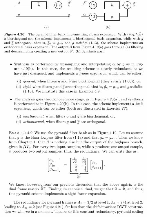
4.5. Wavelet Frames 169
β
α
h 2β′
α
(a)
β′
α
2
2
h
g
+x
(b)
Figure 4.20: The pyramid filter bank implementing a basis expansion. With g, g, h, ha biorthogonal set, the scheme implements a biorthogonal basis expansion, while with gand g orthogonal, that is, gn = g−n and g satisfies (1.13), the scheme implements anorthonormal basis expansion. The output β from Figure 4.19(a) goes through (a) filteringand downsampling creating a new output β′. (b) Synthesis part.
• Synthesis is performed by upsampling and interpolating α by g as in Fig-ure 4.19(b). In this case, the resulting scheme is clearly redundant, as wehave just discussed, and implements a frame expansion, which can be either:
(i) general, when filters g and g are biorthogonal (they satisfy (1.66)), or,
(ii) tight, when filters g and g are orthogonal, that is, gn = g−n and g satisfies(1.13). We illustrate this case in Example 4.9.
• The analysis goes through one more stage, as in Figure 4.20(a), and synthesisis performed as in Figure 4.20(b). In this case, the scheme implements a basisexpansion, which can be either (both are illustrated in Exercise ??):
(i) biorthogonal, when filters g and g are biorthogonal, or,
(ii) orthonormal, when filters g and g are orthogonal.
Example 4.9 We use the pyramid filter bank as in Figure 4.19. Let us assumethat g is the Haar lowpass filter from (1.1a) and that gn = g−n. Then we knowfrom Chapter 1, that β is nothing else but the output of the highpass branch,given in (??). For every two input samples, while α produces one output sample,β produces two output samples; thus, the redundancy. We can write this as:
αnβ2nβ2n+1
=
1√2
1√2
12 − 1
2− 1
212
︸ ︷︷ ︸ΦT
[x2nx2n+1
].
We know, however, from our previous discussion that the above matrix is thedual frame matrix ΦT . Finding its canonical dual, we get that Φ = Φ, and thus,this pyramid scheme implements a tight frame expansion.
The redundancy for pyramid frames is A1 = 3/2 at level 1, A2 = 7/4 at level 2,leading to A∞ = 2 (see Figure 4.21), far less than the shift-invariant DWT construc-tion we will see in a moment. Thanks to this constant redundancy, pyramid coding
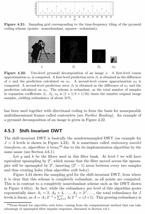
170 Chapter 4. Local Fourier and Wavelet Frames on Sequences
0 2 4 6 8 10 12 14 16 18 20 22 24 26 28 30 32
12345
n
Figure 4.21: Sampling grid corresponding to the time-frequency tiling of the pyramidcoding scheme (points—nonredundant, squares—redundant).
x β1 β2 α2
Figure 4.22: Two-level pyramid decomposition of an image x. A first-level coarseapproximation α1 is computed. A first-level prediction error β1 is obtained as the differenceof x and the prediction calculated on α1. A second-level coarse approximation α2 iscomputed. A second-level prediction error β2 is obtained as the difference of α1 and theprediction calculated on α2. The scheme is redundant, as the total number of samplesin expansion coefficients β1, β2, α2 is (1 + 1/4 + 1/16) times the number original imagesamples, yielding redundancy of about 31%.
has been used together with directional coding to form the basis for nonseparablemultidimensional frames called contourlets (see Further Reading). An example ofa pyramid decomposition of an image is given in Figure 4.22.
4.5.3 Shift-Invariant DWT
The shift-invariant DWT is basically the nondownsampled DWT (an example forJ = 3 levels is shown in Figure 4.23). It is sometimes called stationary wavelettransform, or, algorithme a trous,42 due to the its implementation algorithm by thesame name (see Section 4.6.1).
Let g and h be the filters used in this filter bank. At level ℓ we will haveequivalent upsampling by 2ℓ, which means that the filter moved across the upsam-pler will be upsampled by 2ℓ, inserting (2ℓ − 1) zeros between every two samplesand thus creating holes (thus algorithm with holes).
Figure 4.24 shows the sampling grid for the shift-invariant DWT, from whereit is clear that this scheme is completely redundant, as all points are computed.This is in contrast to a completely nonredundant scheme such as the DWT shownin Figure 4.16(a). In fact, while the redundancy per level of this algorithm growsexponentially since A1 = 2, A2 = 4, . . ., AJ = 2J , . . ., the total redundancy for Jlevels is linear, as A = AJ 2
−J+∑J
ℓ=1Aℓ 2−ℓ = (J+1). This growing redundancy is
42From French for algorithm with holes, coming from the computational method that can takeadvantage of upsampled filter impulse responses, discussed in Section 4.6.1.
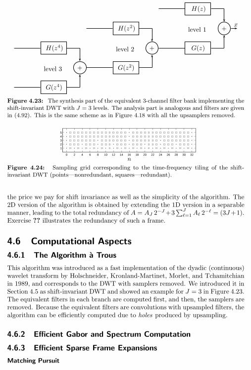
4.6. Computational Aspects 171
H(z4)
G(z4)
level 3 +
H(z2)
G(z2)
level 2 +
H(z)
G(z)
level 1 +x
Figure 4.23: The synthesis part of the equivalent 3-channel filter bank implementing theshift-invariant DWT with J = 3 levels. The analysis part is analogous and filters are givenin (4.92). This is the same scheme as in Figure 4.18 with all the upsamplers removed.
0 2 4 6 8 10 12 14 16 18 20 22 24 26 28 30 32
12345
n
Figure 4.24: Sampling grid corresponding to the time-frequency tiling of the shift-invariant DWT (points—nonredundant, squares—redundant).
the price we pay for shift invariance as well as the simplicity of the algorithm. The2D version of the algorithm is obtained by extending the 1D version in a separablemanner, leading to the total redundancy of A = AJ 2
−J+3∑J
ℓ=1Aℓ 2−ℓ = (3J+1).
Exercise ?? illustrates the redundancy of such a frame.
4.6 Computational Aspects
4.6.1 The Algorithm a Trous
This algorithm was introduced as a fast implementation of the dyadic (continuous)wavelet transform by Holschneider, Kronland-Martinet, Morlet, and Tchamitchianin 1989, and corresponds to the DWT with samplers removed. We introduced it inSection 4.5 as shift-invariant DWT and showed an example for J = 3 in Figure 4.23.The equivalent filters in each branch are computed first, and then, the samplers areremoved. Because the equivalent filters are convolutions with upsampled filters, thealgorithm can be efficiently computed due to holes produced by upsampling.
4.6.2 Efficient Gabor and Spectrum Computation
4.6.3 Efficient Sparse Frame Expansions
Matching Pursuit
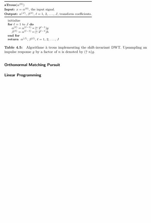
172 Chapter 4. Local Fourier and Wavelet Frames on Sequences
aTrous(α(0))
Input: x = α(0), the input signal.
Output: α(J), β(ℓ), ℓ = 1, 2, . . . , J , transform coefficients.
initializefor ℓ = 1 to J doα(ℓ) = α(ℓ−1) ∗ (↑ 2ℓ−1)gβ(ℓ) = α(ℓ−1) ∗ (↑ 2ℓ−1)h
end forreturn α(J), β(ℓ), ℓ = 1, 2, . . . , J
Table 4.5: Algorithme a trous implementing the shift-invariant DWT. Upsampling animpulse response g by a factor of n is denoted by (↑ n)g.
Orthonormal Matching Pursuit
Linear Programming
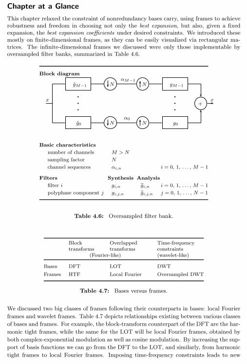
Chapter at a Glance 173
Chapter at a Glance
This chapter relaxed the constraint of nonredundancy bases carry, using frames to achieverobustness and freedom in choosing not only the best expansion, but also, given a fixedexpansion, the best expansion coefficients under desired constraints. We introduced thesemostly on finite-dimensional frames, as they can be easily visualized via rectangular ma-trices. The infinite-dimensional frames we discussed were only those implementable byoversampled filter banks, summarized in Table 4.6.
Block diagram
x
gM−1
g0
b
b
b
N
N
αM−1
α0
N
N
gM−1
g0
b
b
b
+x
Basic characteristics
number of channels M > N
sampling factor N
channel sequences αi,n i = 0, 1, . . . , M − 1
Filters Synthesis Analysis
filter i gi,n gi,n i = 0, 1, . . . , M − 1
polyphase component j gi,j,n gi,j,n j = 0, 1, . . . , N − 1
Table 4.6: Oversampled filter bank.
Block Overlapped Time-frequencytransforms transforms constraints
(Fourier-like) (wavelet-like)
Bases DFT LOT DWT
Frames HTF Local Fourier Oversampled DWT
Table 4.7: Bases versus frames.
We discussed two big classes of frames following their counterparts in bases: local Fourier
frames and wavelet frames. Table 4.7 depicts relationships existing between various classes
of bases and frames. For example, the block-transform counterpart of the DFT are the har-
monic tight frames, while the same for the LOT will be local Fourier frames, obtained by
both complex-exponential modulation as well as cosine modulation. By increasing the sup-
port of basis functions we can go from the DFT to the LOT, and similarly, from harmonic
tight frames to local Fourier frames. Imposing time-frequency constraints leads to new
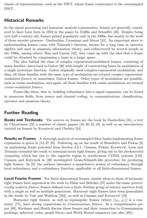
174 Chapter 4. Local Fourier and Wavelet Frames on Sequences
classes of representations, such as the DWT, whose frame counterpart is the oversampled
DWT.
Historical Remarks
In the signal processing and harmonic analysis communities, frames are generally consid-ered to have been born in 1952 in the paper by Duffin and Schaeffer [36]. Despite beingover half a century old, frames gained popularity only in the 1990s, due mostly to the workof three wavelet pioneers—Daubechies, Grossman and Meyer [32]. An important piece tounderstanding frames came with Naimark’s theorem, known for a long time in operatoralgebra and used in quantum information theory, and rediscovered by several people inthe 1990s, among others, Han and Larson [42]; they came up with the idea that a framecould be obtained by compressing a basis in a larger space.
The idea behind the class of complex exponential-modulated frames, consisting ofmany families, dates back to Gabor [40] with insight of constructing bases by modulation ofa single prototype function. Gabor originally used complex-exponential modulation, andthus, all those families with the same type of modulation are termed complex exponential-modulated frames, or sometimes, Gabor frames. Other types of modulation are possible,such as cosine modulation, and again, all those families with cosine modulation are termedcosine-modulated frames.
Frame-like ideas, that is, building redundancy into a signal expansion, can be found
in numerous fields, from source and channel coding, to communications, classification,
operator and quantum theory.
Further Reading
Books and Textbooks The sources on frames are the book by Daubechies [31], a textby Christensen [22] a number of classic papers [18, 30, 42, 43] as well as an introductorytutorial on frames by Kovacevic and Chebira [54].
Results on Frames A thorough analysis of oversampled filter banks implementing frameexpansions is given in [12, 27, 28]. Following up on the result of Benedetto and Fickus [8]on minimizing frame potential from Section 4.2.1, Cassaza, Fickus, Kovacevic, Leon andTremain extended the result to nonequal-norm tight frames, giving rise to the fundamentalinequality, which has ties to the capacity region in synchronous CDMA systems [110].Casazza and Kutyniok in [20] investigated Gram-Schmidt-like procedure for producingtight frames. In [9], the authors introduce a quantitative notion of redundancy throughlocal redundancy and a redundancy function, applicable to all finite-dimensional frames.
Local Fourier Frames For finite-dimensional frames, similar ideas to those of harmonictight frames have appeared in the work by Eldar and Bolcskei [37] under the name geomet-rically uniform frames, frames defined over a finite Abelian group of unitary matrices bothwith a single as well as multiple generators. Harmonic tight frames have been generalizedin the works by Vale and Waldron [102], as well as Casazza and Kovacevic [19].
Harmonic tight frames, as well as equiangular frames (where |〈ϕi, ϕj〉| is a con-stant) [71], have strong connections to Grassmannian frames. In a comprehensive pa-per [89], Strohmer and Heath discuss those frames and their connection to Grassmannianpackings, spherical codes, graph theory and Welch Bound sequences (see also [48]).
Further Reading 175
The lack of infinite-dimensional bases with good time and frequency localization,the result of the discrete Balian-Low theorem, prompted the development of oversampledfilter banks that use complex-exponential modulation. They are known under variousnames: oversampled DFT filter banks, complex exponential-modulated filter banks, short-time Fourier filter banks and Gabor filter banks and have been studied in [10–12,26,39,88].Bolcskei and Hlawatsch in [11] have studied the other type of modulation, cosine. Theconnection between these two classes is deep as there exists a general decomposition ofthe frame operator corresponding to a cosine-modulated filter bank as the sum of theframe operator of the underlying complex exponential-modulated frame and an additionaloperator, which vanishes under certain conditions [6]. The lapped tight frame transformswere proposed as a way to obtain a large number of frames by seeding from LOTs [21,76].
Wavelet Frames Apart from those already discussed, like pyramid frames [15], manyother wavelet-like frame families have been proposed, among them, the dual-tree complexwavelet transform, a nearly shift-invariant transform with redundancy of only 2, intro-duced by Kingsbury [51–53]. Selesnick in [77, 78] followed with the double-density DWTand variations, which can approximately be implemented using a 3-channel filter bank withsampling by 2, again nearly shift invariant with redundancy that tends towards 2 wheniterated. Some other variations include power-shiftable DWT [81] or partial DWT [85],which removes samplers at the first level but leaves them at all other levels, with redun-dancy Aj = 2 at each level and again near shift invariance. Bradley in [13] introduces theovercomplete DWT, the DWT with critical sampling for the first k levels followed by theshift-invariant DWT for the last j − k levels.
Multidimensional Frames Apart from obvious, tensor-like, constructions of multidi-mensional frames, true multidimensional solutions exist. The oldest multidimensionalframe seems to be the steerable pyramid introduced by Simoncelli, Freeman, Adelsonand Heeger in 1992 [81], following on the previous work by Burt and Adelson on pyra-mid coding [15]. The steerable pyramid possesses many nice properties, such as jointspace-frequency localization, approximate shift invariance, approximate tightness and ap-proximate rotation invariance. An excellent overview of the steerable pyramid and itsapplications is given on Simoncelli’s web page [80].
Another multidimensional example is the work of Do and Vetterli on contourlets [25,34], motivated by the need to construct efficient and sparse representations of intrinsicgeometric structure of information within an image. The authors combine the ideas ofpyramid filter banks [33] with directional processing, to obtain contourlets, expansionscapturing contour segments. These are almost critically sampled, with redundancy of1.33.
Some other examples include [58] where the authors build both critically-sampledand shift-invariant 2D DWT. Many ”-lets” are also multidimensional frames, such ascurvelets [16,17] and shearlets [56]. As the name implies, curvelets are used to approximatecurved singularities in an efficient manner [16, 17]. As opposed to wavelets, which usedilation and translation, shearlets use dilation, shear transformation and translation, andpossess useful properties such as directionality, elongated shapes and many others [56].
Applications of Frames Frames have become extremely popular and have been used in
many application fields. The text by Kovacevic and Chebira [54] contains an overview of
many of these and a number of relevant references. In some fields, frames have been used
for years, for example in CDMA systems, in the work of Massey and Mittelholzer [63] on

176 Chapter 4. Local Fourier and Wavelet Frames on Sequences
Welch bound and sequence sets for CDMA systems. It turns out that the Welch bound is
equivalent to the frame potential minimization inequality. The equivalence between unit-
norm tight frames and Welch bound sequences was shown in [89]. Waldron formalized that
equivalence for general tight frames in [111], and consequently, tight frames are referred
in some works as Welch bound sequences [92].
Chapter 5
Local Fourier Transforms,
Frames and Bases on
Functions
Contents
5.1 Introduction 178
5.2 Local Fourier Transform 178
5.3 Local Fourier Frame Series 188
5.4 Local Fourier Series 188
5.5 Computational Aspects 188
Chapter at a Glance 188
Historical Remarks 188
Further Reading 188
Dear Reader,
This chapter needs to be finished. The only existing section, Section 5.2has been proofread and integrated with the previous text. The rest of thesections are yet to be written.
Please read on. — MV, JK, and VKG
The aim of this chapter follows that of Chapter 2, but for functions. Welook for ways to localize the analysis Fourier transform provides by windowingthe complex exponentials. As before, this will improve the time localization ofthe corresponding transform at the expense of the frequency localization. Theoriginal idea dates back to Gabor, and thus Gabor transform is frequently used;windowed Fourier transform and short-time Fourier transform are as well. Wechoose the intuitive local Fourier transform, as a counterpart to local Fourier basesfrom Chapter 2 and local Fourier frames from Chapter 4.
We start with the most redundant one, local Fourier transform, and thensample to obtain local Fourier frames. With critical sampling we then try for localFourier bases, where, not surprisingly after what we have seen in Chapter 2, baseswith simultaneously good time and frequency localization do not exist, the result
177
178 Chapter 5. Local Fourier Transforms, Frames and Bases on Functions
known as Balian-Low theorem. Again as in Chapter 2, cosine local Fourier basesdo exist, as do wavelet ones we discuss in the next chapter.
5.1 Introduction
Fourier Series Basis Expansion
Localization Properties of the Fourier Series
Chapter Outline
We start with the most redundant one version of the local Fourier transform, thelocal Fourier transform in Section 5.2, and then sample to obtain local Fourierframes in Section 5.3. With critical sampling we then try for local Fourier bases inSection 5.4, where, not surprisingly after what we have seen in Chapter 2, complexexponential-modulated local Fourier bases with simultaneously good time and fre-quency localization do not exist, the result known as Balian-Low theorem. Againas in Chapter 2, cosine-modulated local Fourier bases do exist, as do wavelet oneswe discuss in the next chapter.
Notation used in this chapter: The prototype window function in this chapter isnamed p(t); this is for consistency with the prototype window sequences used inChapters 2 and 4; g(t) is more commonly seen in the literature.
5.2 Local Fourier Transform
Given a function x(t), we start with its Fourier transformX(ω) as in Definition 4.10.We analyze x(t) locally by using a prototype window function p(t). We will assumep(t) is symmetric, p(t) = p(−t), and real. The prototype function should be smoothas well, in particular, it should be smoother than the function to be analyzed.43
5.2.1 Definition of the Local Fourier Transform
We can look at our windowing with the prototype function p(t) in two ways:
(i) We window the function x(t) as
xτ (t) = p(t− τ)x(t), (5.1)
and then take its Fourier transform (4.42a),
Xτ (ω) = 〈xτ , vω〉 =
∫
t∈R
xτ (t) e−jωt dt =
∫
t∈R
x(t) p(t−τ)e−jωt dt, (5.2)
for ω ∈ R.
43Otherwise, it will interfere with the smoothness of the function to be analyzed; see Sec-tion 5.2.2.
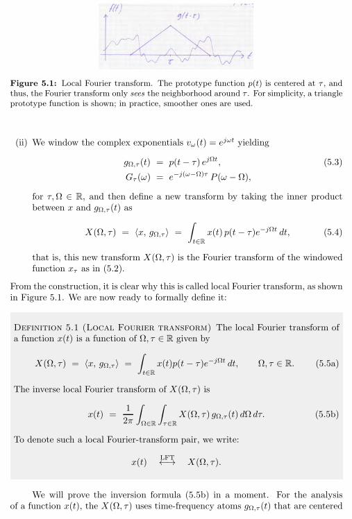
5.2. Local Fourier Transform 179
Figure 5.1: Local Fourier transform. The prototype function p(t) is centered at τ , andthus, the Fourier transform only sees the neighborhood around τ . For simplicity, a triangleprototype function is shown; in practice, smoother ones are used.
(ii) We window the complex exponentials vω(t) = ejωt yielding
gΩ,τ (t) = p(t− τ) ejΩt, (5.3)
Gτ (ω) = e−j(ω−Ω)τ P (ω − Ω),
for τ,Ω ∈ R, and then define a new transform by taking the inner productbetween x and gΩ,τ (t) as
X(Ω, τ) = 〈x, gΩ,τ 〉 =
∫
t∈R
x(t) p(t− τ)e−jΩt dt, (5.4)
that is, this new transform X(Ω, τ) is the Fourier transform of the windowedfunction xτ as in (5.2).
From the construction, it is clear why this is called local Fourier transform, as shownin Figure 5.1. We are now ready to formally define it:
Definition 5.1 (Local Fourier transform) The local Fourier transform ofa function x(t) is a function of Ω, τ ∈ R given by
X(Ω, τ) = 〈x, gΩ,τ 〉 =
∫
t∈R
x(t)p(t − τ)e−jΩt dt, Ω, τ ∈ R. (5.5a)
The inverse local Fourier transform of X(Ω, τ) is
x(t) =1
2π
∫
Ω∈R
∫
τ∈R
X(Ω, τ) gΩ,τ (t) dΩ dτ. (5.5b)
To denote such a local Fourier-transform pair, we write:
x(t)LFT←→ X(Ω, τ).
We will prove the inversion formula (5.5b) in a moment. For the analysisof a function x(t), the X(Ω, τ) uses time-frequency atoms gΩ,τ (t) that are centered
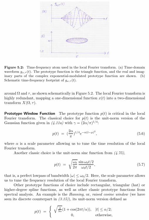
180 Chapter 5. Local Fourier Transforms, Frames and Bases on Functions
Figure 5.2: Time-frequency atom used in the local Fourier transform. (a) Time-domainwaveform gω,τ (t). The prototype function is the triangle function, and the real and imag-inary parts of the complex exponential-modulated prototype function are shown. (b)Schematic time-frequency footprint of gω,τ (t).
around Ω and τ , as shown schematically in Figure 5.2. The local Fourier transform ishighly redundant, mapping a one-dimensional function x(t) into a two-dimensionaltransform X(Ω, τ).
Prototype Window Function The prototype function p(t) is critical in the localFourier transform. The classical choice for p(t) is the unit-norm version of theGaussian function given in (4.11a) with γ = (2α/π)1/4:
p(t) = (2α
π)1/4e−α(t−µ)
2
, (5.6)
where α is a scale parameter allowing us to tune the time resolution of the localFourier transform.
Another classic choice is the unit-norm sinc function from (4.75),
p(t) =
√ω0
2π
sinω0t/2
ω0t/2, (5.7)
that is, a perfect lowpass of bandwidth |ω| ≤ ω0/2. Here, the scale parameter allowsus to tune the frequency resolution of the local Fourier transform.
Other prototype functions of choice include rectangular, triangular (hat) orhigher-degree spline functions, as well as other classic prototype functions fromspectral analysis. An example is the Hanning, or, raised cosine window (we haveseen its discrete counterpart in (3.15)), its unit-norm version defined as
p(t) =
√23α (1 + cos(2πt/α)), |t| ≤ α/2;
0, otherwise,
5.2. Local Fourier Transform 181
where α is a scale parameter.44
Inversion of the Local Fourier Transform While we have taken for granted thatthe inversion formula (5.5b) holds, this is not a given. However, given the redun-dancy present in the local Fourier transform, we expect such an inversion to bepossible, which we now prove.
We are going to apply the generalized Parseval’s equality to (5.5b), and wethus need the Fourier transform of X(Ω, τ) with respect to τ . We have that
X(Ω, τ) =
∫
t∈R
x(t) p(t− τ) e−jΩt dt,
(a)=
∫
t∈R
p(τ − t)x(t) e−jΩt dt (b)= (p ∗ xΩ)(τ),
where (a) follows from p(t) = p(−t), and in (b) we introduced xΩ(t) = x(t)e−jΩt.Using the shift-in-frequency property (4.54), the Fourier transform of xΩ(t) isX(ω+Ω). Then, using the convolution property (4.61), the Fourier transform of X(Ω, τ)with respect to τ becomes,
X(Ω, ω) = P (ω)X(ω +Ω). (5.8)
In (5.5b), the other term involving τ is gΩ,τ (t) = p(t − τ)ejΩt. Using theshift-in-time property (4.53) and because p(t) is symmetric, the Fourier transformof p(t− τ) with respect to τ is
p(t− τ) FT←→ e−jωtP (ω). (5.9)
We now apply the generalized Parseval’s equality (4.70b) to the right side of (5.5b):
1
2π
∫
Ω∈R
(∫
τ∈R
X(Ω, τ) p(t− τ) ejΩt dτ)dΩ
(a)=
1
2π
∫
Ω∈R
(1
2π
∫
ω∈R
X(ω +Ω)P (ω)P ∗(ω) ejωtejΩt dω
)dΩ
(b)=
1
2π
∫
ω∈R
|P (ω)|2(
1
2π
∫
Ω∈R
X(ω +Ω)ej(ω+Ω)t dΩ
)dω,
(c)= x(t)
1
2π
∫
ω∈R
|P (ω)|2 dω (d)= x(t).
where (a) follows from (5.8), (5.9) and generalized Parseval’s equality (4.70b); (b)from Fubini’s theorem (see Appendix 2.A.3) allowing for the exchange of the orderof integration; (c) from the inverse Fourier transform (4.42b); and (d) from p beingof unit norm and Parseval’s equality (4.70a).
44In the signal processing literature, the normalization factor is usually 1/2, such that p(0) = 1.
182 Chapter 5. Local Fourier Transforms, Frames and Bases on Functions
5.2.2 Properties of the Local Fourier Transform
We now look into the main properties of the local Fourier transform, includingenergy conservation, followed by basic characteristics such as localization propertiesand examples, including spectrograms, which are density plots of the magnitude ofthe local Fourier transform.
TBD: Table with properties.
Linearity The local Fourier transform operator is a linear operator, or,
αx(t) + β y(t)LFT←→ αX(Ω, τ) + β Y (Ω, τ). (5.10)
Shift in Time A shift in time by t0 results in
x(t− t0) LFT←→ e−jΩt0X(Ω, τ − t0). (5.11)
This is to be expected as it follows from the shift-in-time property of the Fouriertransform, (4.53). To see that,∫
t∈R
p(t− τ)x(t − t0) e−jΩt dt(a)= e−jΩt0
∫
t′∈R
p(t′ − (τ − t0))x(t′)e−jΩt′
dt′
(b)= e−jΩt0X(Ω, τ − t0),
where (a) follows from change of variable t′ = t− t0; and (b) from the definition ofthe local Fourier transform (5.5a). Thus, a shift by t0 simply shifts the local Fouriertransform and adds a phase factor. The former illustrates the locality of the localFourier transform, while the latter follows from the equivalent Fourier-transformproperty.
Shift in Frequency A shift in frequency by ω0 results in
ejω0t x(t)LFT←→ X(Ω− ω0, τ). (5.12)
To see this,∫
t∈R
p(t− τ) ejω0t x(t) e−jΩt dt
=
∫
t∈R
p(t− τ)x(t) e−j(Ω−ω0)t dt = X(Ω− ω0, τ),
the same as for the Fourier transform. As before, a shift in frequency is oftenreferred to as modulation, and is dual to the shift in time.
Parseval’s Equality The local Fourier-transform operator is a unitary operatorand thus preserves the Euclidean norm (see (2.53)):
‖x‖2 =
∫
t∈R
|x(t)|2 dt =1
2π
∫
Ω∈R
∫
τ∈R
|X(Ω, τ)|2 dΩ dτ =1
2π‖X‖2. (5.13)
5.2. Local Fourier Transform 183
We now prove Parseval’s equality for functions that are both in L1 and L2: Itshould come as no surprise that to derive Parseval’s equality for the local Fouriertransform, we use Parseval’s equality for the Fourier transform. Start with the rightside of (5.13) to get
1
2π
∫
τ∈R
∫
Ω∈R
|X(Ω, τ)|2 dΩ dτ
(a)=
1
2π
∫
Ω∈R
(1
2π
∫
ω∈R
|X(ω +Ω)P (ω)|2 dω)dΩ
(b)=
1
2π
∫
ω∈R
|P (ω)|2(
1
2π
∫
Ω∈R
|X(ω +Ω)|2dΩ)dω,
(c)= ‖x‖2 1
2π
∫
ω∈R
|P (ω)|2 dω (d)= ‖x‖2,
where (a) follows from Parseval’s equality (4.70a) and (5.8); (b) from Fubini’stheorem (see Appendix 2.A.3) allowing for the exchange of the order of integration;(c) from the inverse Fourier transform (4.42b); and (d) from p being of unit normand Parseval’s equality (4.70a).
Redundancy The local Fourier transform maps a function of one variable intoa function of two variables. It is thus highly redundant, and this redundancy isexpressed by the reproducing kernel :
K(Ω, τ, ω0, t0) = 〈gΩ,τ , gω0,t0〉
=
∫
t∈R
p(t− τ)p(t− t0) ej(ω0−Ω)t dt. (5.14)
While this is a four-dimensional object, its magnitude depends only on the twodifferences (ω0 − Ω) and (t0 − τ).45
Theorem 5.2 (Reproducing kernel formula for the local Fourier transform)A function X(ω0, t0) is the local Fourier transform of some function x(t) if andonly if it satisfies
X(Ω, τ) =1
2π
∫
t1∈R
∫
ω0∈R
X(ω0, t0)K(Ω, τ, ω0, t0) dω0 dt0. (5.15)
Proof. If X(ω0, t0) is a local Fourier transform, then there is a function x(t) such that
45This is expressed in a closely related function called the ambiguity function; see Exercise ??.
184 Chapter 5. Local Fourier Transforms, Frames and Bases on Functions
X(ω0, t0) = X(ω0, t0), or
X(Ω, τ ) =
∫
t∈R
x(t) g∗Ω,τ (t) dt,
(a)=
∫
t∈R
(1
2π
∫
t0∈R
∫
ω0∈R
X(ω0, t0)gω0,t0(t) dω0 dt0
)g∗Ω,τ (t) dt
=1
2π
∫
t0∈R
∫
ω0∈R
X(ω0, t0)
(∫
t∈R
gΩ,τ (t)gω0,t0(t) dt
)dω0 dt0,
(b)=
1
2π
∫
t0∈R
∫
ω0∈R
X(ω0, t0)K(Ω, τ, ω0, t0)dω0 dt0,
(5.5b) where (a) follows from the inversion formula (5.5b) and (b) from (5.15).For the converse, write (5.15) by making K(Ω, τ, ω0, t0) explicit as an integral
over t (see (5.14)):
X(Ω, τ ) =1
2π
∫
t1∈R
∫
ω1∈R
∫
t∈R
X(ω0, t0) gΩ,τ (t) gω,t(t) dt dω0 dt0
(a)=
∫
t∈R
gΩ,τ (t)
(1
2π
∫
t1∈R
∫
ω1∈R
X(ω0, t0) gω,t(t) dω0 dt0
)dt
(b)=
∫
t∈R
gΩ,τ (t)x(t) dt,
where (a) follows from Fubini’s theorem (see Appendix 2.A.3) allowing for the exchangeof the order of integration, and (b) from the inversion formula (5.5b). Therefore, X(Ω, τ )is indeed a local Fourier transform, namely the local Fourier transform of x(t).
The redundancy present in the local Fourier transform allows sampling and inter-polation, and the interpolation kernel depends on the reproducing kernel.
Characterization of Singularities and Smoothness To characterize singularities,we will take the view that the local Fourier transform is a Fourier transform of awindowed function xτ (t) as in (5.1). Since this is a product between the functionand the prototype function, using the convolution-in-frequency property (4.64), inthe Fourier domain this is a convolution. That is, singularities are smoothed by theprototype function.
We now characterization of singularities in time and frequency, depicted inFigure 5.3.
(i) Characterization of singularities in time: Take a function perfectly localizedin time, the Dirac delta function x(t) = δ(t− t0). Then
X(Ω, τ) =
∫
t∈R
p(t− τ) δ(t− t0) e−jΩt dt(a)= p(t0 − τ) e−jΩt0 ,
where (a) follows from Table 4.1. This illustrates the characterization of sin-gularities in time by the local Fourier transform: An event at time locationt0 will spread around t0 according to the prototype function, and this acrossall frequencies. If p(t) has compact support [−T/2, T/2], then X(Ω, τ) hassupport [−∞,∞]× [t0 − T/2, t0 + T/2].
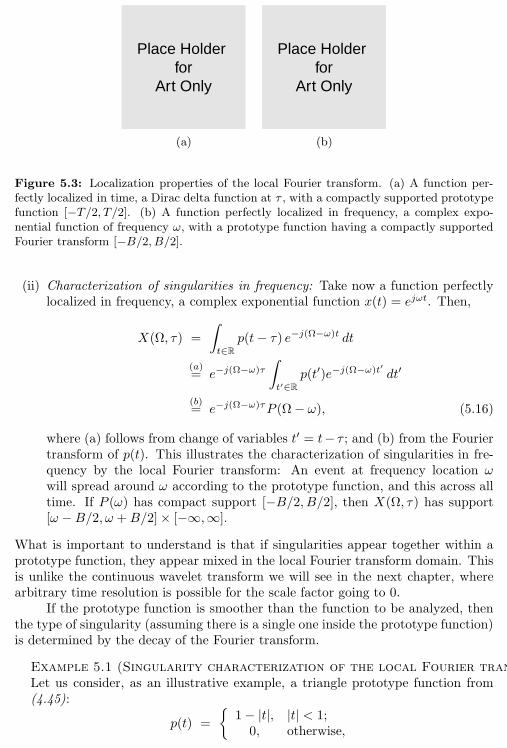
5.2. Local Fourier Transform 185
Place Holder for
Art Only
Place Holder for
Art Only
(a) (b)
Figure 5.3: Localization properties of the local Fourier transform. (a) A function per-fectly localized in time, a Dirac delta function at τ , with a compactly supported prototypefunction [−T/2, T/2]. (b) A function perfectly localized in frequency, a complex expo-nential function of frequency ω, with a prototype function having a compactly supportedFourier transform [−B/2, B/2].
(ii) Characterization of singularities in frequency: Take now a function perfectlylocalized in frequency, a complex exponential function x(t) = ejωt. Then,
X(Ω, τ) =
∫
t∈R
p(t− τ) e−j(Ω−ω)t dt
(a)= e−j(Ω−ω)τ
∫
t′∈R
p(t′)e−j(Ω−ω)t′ dt′
(b)= e−j(Ω−ω)τP (Ω− ω), (5.16)
where (a) follows from change of variables t′ = t− τ ; and (b) from the Fouriertransform of p(t). This illustrates the characterization of singularities in fre-quency by the local Fourier transform: An event at frequency location ωwill spread around ω according to the prototype function, and this across alltime. If P (ω) has compact support [−B/2, B/2], then X(Ω, τ) has support[ω −B/2, ω +B/2]× [−∞,∞].
What is important to understand is that if singularities appear together within aprototype function, they appear mixed in the local Fourier transform domain. Thisis unlike the continuous wavelet transform we will see in the next chapter, wherearbitrary time resolution is possible for the scale factor going to 0.
If the prototype function is smoother than the function to be analyzed, thenthe type of singularity (assuming there is a single one inside the prototype function)is determined by the decay of the Fourier transform.
Example 5.1 (Singularity characterization of the local Fourier transform)Let us consider, as an illustrative example, a triangle prototype function from(4.45):
p(t) =
1− |t|, |t| < 1;
0, otherwise,
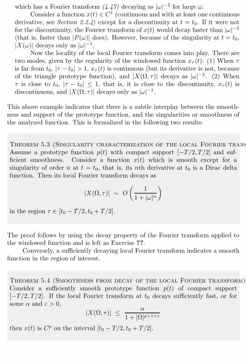
186 Chapter 5. Local Fourier Transforms, Frames and Bases on Functions
which has a Fourier transform (4.47) decaying as |ω|−2 for large ω.Consider a function x(t) ∈ C1 (continuous and with at least one continuous
derivative, see Section 2.2.4) except for a discontinuity at t = t0. If it were notfor the discontinuity, the Fourier transform of x(t) would decay faster than |ω|−2
(that is, faster than |P (ω)| does). However, because of the singularity at t = t0,|X(ω)| decays only as |ω|−1.
Now the locality of the local Fourier transform comes into play. There aretwo modes, given by the regularity of the windowed function xτ (t): (1) When τis far from t0, |τ − t0| > 1, xτ (t) is continuous (but its derivative is not, becauseof the triangle prototype function), and |X(Ω, τ)| decays as |ω|−2. (2) Whenτ is close to t0, |τ − t0| ≤ 1, that is, it is close to the discontinuity, xτ (t) isdiscontinuous, and |X(Ω, τ)| decays only as |ω|−1.
This above example indicates that there is a subtle interplay between the smooth-ness and support of the prototype function, and the singularities or smoothness ofthe analyzed function. This is formalized in the following two results:
Theorem 5.3 (Singularity characterization of the local Fourier transform)Assume a prototype function p(t) with compact support [−T/2, T/2] and suf-ficient smoothness. Consider a function x(t) which is smooth except for asingularity of order n at t = t0, that is, its nth derivative at t0 is a Dirac deltafunction. Then its local Fourier transform decays as
|X(Ω, τ)| ∼ O
(1
1 + |ω|n)
in the region τ ∈ [t0 − T/2, t0 + T/2].
The proof follows by using the decay property of the Fourier transform applied tothe windowed function and is left as Exercise ??.
Conversely, a sufficiently decaying local Fourier transform indicates a smoothfunction in the region of interest.
Theorem 5.4 (Smoothness from decay of the local Fourier transform)Consider a sufficiently smooth prototype function p(t) of compact support[−T/2, T/2]. If the local Fourier transform at t0 decays sufficiently fast, or forsome α and ε > 0,
|X(Ω, τ)| ≤ α
1 + |Ω|p+1+ε
then x(t) is Cp on the interval [t0 − T/2, t0 + T/2].
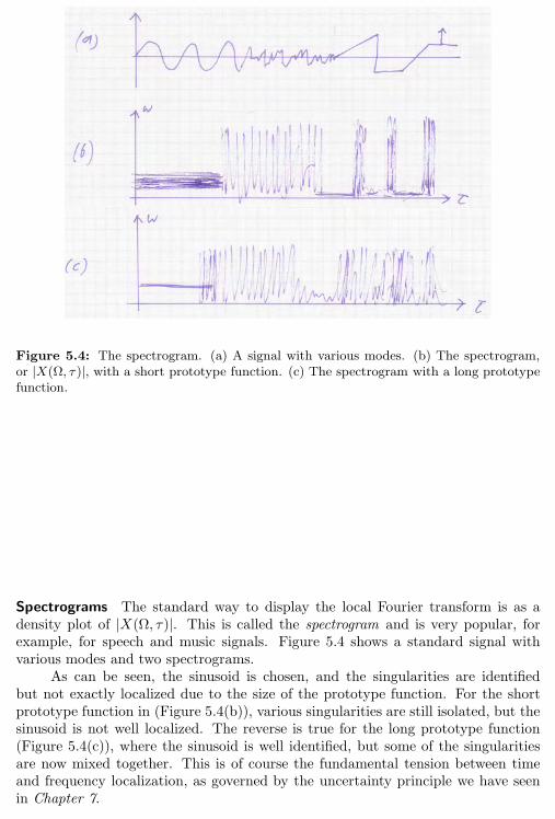
5.2. Local Fourier Transform 187
Figure 5.4: The spectrogram. (a) A signal with various modes. (b) The spectrogram,or |X(Ω, τ )|, with a short prototype function. (c) The spectrogram with a long prototypefunction.
Spectrograms The standard way to display the local Fourier transform is as adensity plot of |X(Ω, τ)|. This is called the spectrogram and is very popular, forexample, for speech and music signals. Figure 5.4 shows a standard signal withvarious modes and two spectrograms.
As can be seen, the sinusoid is chosen, and the singularities are identifiedbut not exactly localized due to the size of the prototype function. For the shortprototype function in (Figure 5.4(b)), various singularities are still isolated, but thesinusoid is not well localized. The reverse is true for the long prototype function(Figure 5.4(c)), where the sinusoid is well identified, but some of the singularitiesare now mixed together. This is of course the fundamental tension between timeand frequency localization, as governed by the uncertainty principle we have seenin Chapter 7.
188 Chapter 5. Local Fourier Transforms, Frames and Bases on Functions
5.3 Local Fourier Frame Series
5.3.1 Sampling Grids
5.3.2 Frames from Sampled Local Fourier Transform
5.4 Local Fourier Series
5.4.1 Complex Exponential-Modulated Local Fourier Bases
Complex-Exponential Modulation
Balian-Low Theorem
5.4.2 Cosine-Modulated Local Fourier Bases
Cosine Modulation
Local Cosine Bases
5.5 Computational Aspects
5.5.1 Complex Exponential-Modulated Local Fourier Bases
5.5.2 Cosine-Modulated Local Fourier Bases
Chapter at a Glance
TBD
Historical Remarks
TBD
Further Reading
TBD
Chapter 6
Wavelet Bases, Frames
and Transforms on
Functions
Contents
6.1 Introduction 189
6.2 Scaling Function and Wavelets from OrthogonalFilter Banks 208
6.3 Wavelet Series 222
6.4 Wavelet Frame Series 242
6.5 Continuous Wavelet Transform 242
6.6 Computational Aspects 254
Chapter at a Glance 259
Historical Remarks 259
Further Reading 259
The previous chapter started with the most redundant version of the localFourier expansions on functions: the local Fourier transform. We lowered its re-dundancy through sampling, leading to Fourier frames. Ultimately, we wanted tomake it nonredundant by trying to build local Fourier bases; however, we hit aroadblock, the Balian-Low theorem, prohibiting such bases with reasonable jointtime and frequency localization. While bases are possible with cosine, instead ofcomplex-exponential, modulation, we can do even better. In this chapter, we willstart by constructing wavelet bases, and then go in the direction of increasing re-dundancy, by building frames and finally the continuous wavelet transform.
6.1 Introduction
Iterated filter banks from Chapter 3 pose interesting theoretical and practical ques-tions, the key one quite simple: what happens if we iterate the DWT to infinity?While we need to make the question precise by indicating how this iterative processtakes place, when done properly, and under certain conditions on the filters used inthe filter bank, the limit leads to a wavelet basis for the space of square-integrable
189
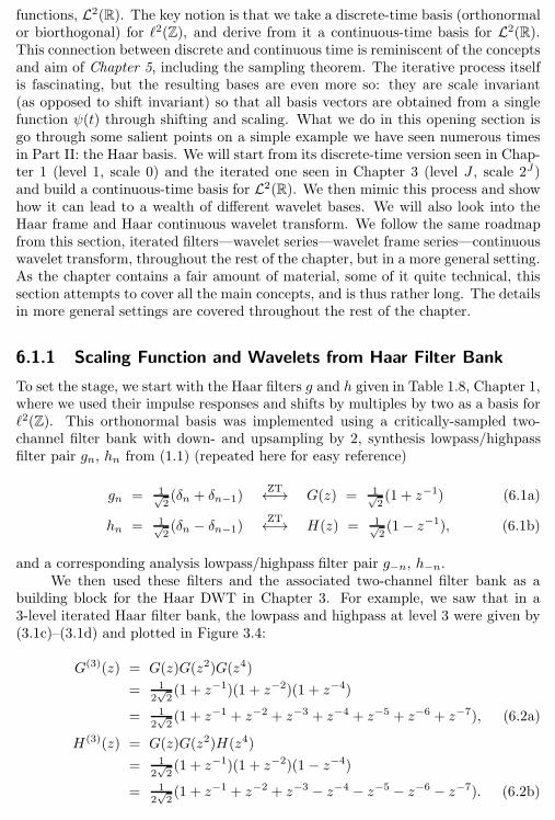
190 Chapter 6. Wavelet Bases, Frames and Transforms on Functions
functions, L2(R). The key notion is that we take a discrete-time basis (orthonormalor biorthogonal) for ℓ2(Z), and derive from it a continuous-time basis for L2(R).This connection between discrete and continuous time is reminiscent of the conceptsand aim of Chapter 5, including the sampling theorem. The iterative process itselfis fascinating, but the resulting bases are even more so: they are scale invariant(as opposed to shift invariant) so that all basis vectors are obtained from a singlefunction ψ(t) through shifting and scaling. What we do in this opening section isgo through some salient points on a simple example we have seen numerous timesin Part II: the Haar basis. We will start from its discrete-time version seen in Chap-ter 1 (level 1, scale 0) and the iterated one seen in Chapter 3 (level J , scale 2J)and build a continuous-time basis for L2(R). We then mimic this process and showhow it can lead to a wealth of different wavelet bases. We will also look into theHaar frame and Haar continuous wavelet transform. We follow the same roadmapfrom this section, iterated filters—wavelet series—wavelet frame series—continuouswavelet transform, throughout the rest of the chapter, but in a more general setting.As the chapter contains a fair amount of material, some of it quite technical, thissection attempts to cover all the main concepts, and is thus rather long. The detailsin more general settings are covered throughout the rest of the chapter.
6.1.1 Scaling Function and Wavelets from Haar Filter Bank
To set the stage, we start with the Haar filters g and h given in Table 1.8, Chapter 1,where we used their impulse responses and shifts by multiples by two as a basis forℓ2(Z). This orthonormal basis was implemented using a critically-sampled two-channel filter bank with down- and upsampling by 2, synthesis lowpass/highpassfilter pair gn, hn from (1.1) (repeated here for easy reference)
gn = 1√2(δn + δn−1)
ZT←→ G(z) = 1√2(1 + z−1) (6.1a)
hn = 1√2(δn − δn−1)
ZT←→ H(z) = 1√2(1− z−1), (6.1b)
and a corresponding analysis lowpass/highpass filter pair g−n, h−n.We then used these filters and the associated two-channel filter bank as a
building block for the Haar DWT in Chapter 3. For example, we saw that in a3-level iterated Haar filter bank, the lowpass and highpass at level 3 were given by(3.1c)–(3.1d) and plotted in Figure 3.4:
G(3)(z) = G(z)G(z2)G(z4)
= 12√2(1 + z−1)(1 + z−2)(1 + z−4)
= 12√2(1 + z−1 + z−2 + z−3 + z−4 + z−5 + z−6 + z−7), (6.2a)
H(3)(z) = G(z)G(z2)H(z4)
= 12√2(1 + z−1)(1 + z−2)(1 − z−4)
= 12√2(1 + z−1 + z−2 + z−3 − z−4 − z−5 − z−6 − z−7). (6.2b)
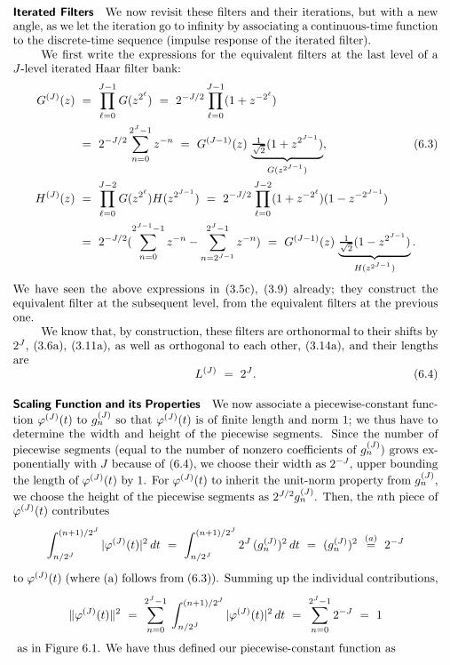
6.1. Introduction 191
Iterated Filters We now revisit these filters and their iterations, but with a newangle, as we let the iteration go to infinity by associating a continuous-time functionto the discrete-time sequence (impulse response of the iterated filter).
We first write the expressions for the equivalent filters at the last level of aJ-level iterated Haar filter bank:
G(J)(z) =
J−1∏
ℓ=0
G(z2ℓ
) = 2−J/2J−1∏
ℓ=0
(1 + z−2ℓ)
= 2−J/22J−1∑
n=0
z−n = G(J−1)(z) 1√2(1 + z2
J−1
)︸ ︷︷ ︸
G(z2J−1)
, (6.3)
H(J)(z) =
J−2∏
ℓ=0
G(z2ℓ
)H(z2J−1
) = 2−J/2J−2∏
ℓ=0
(1 + z−2ℓ)(1 − z−2J−1
)
= 2−J/2(2J−1−1∑
n=0
z−n −2J−1∑
n=2J−1
z−n) = G(J−1)(z) 1√2(1− z2J−1
)︸ ︷︷ ︸
H(z2J−1 )
.
We have seen the above expressions in (3.5c), (3.9) already; they construct theequivalent filter at the subsequent level, from the equivalent filters at the previousone.
We know that, by construction, these filters are orthonormal to their shifts by2J , (3.6a), (3.11a), as well as orthogonal to each other, (3.14a), and their lengthsare
L(J) = 2J . (6.4)
Scaling Function and its Properties We now associate a piecewise-constant func-
tion ϕ(J)(t) to g(J)n so that ϕ(J)(t) is of finite length and norm 1; we thus have to
determine the width and height of the piecewise segments. Since the number of
piecewise segments (equal to the number of nonzero coefficients of g(J)n ) grows ex-
ponentially with J because of (6.4), we choose their width as 2−J , upper bounding
the length of ϕ(J)(t) by 1. For ϕ(J)(t) to inherit the unit-norm property from g(J)n ,
we choose the height of the piecewise segments as 2J/2g(J)n . Then, the nth piece of
ϕ(J)(t) contributes
∫ (n+1)/2J
n/2J|ϕ(J)(t)|2 dt =
∫ (n+1)/2J
n/2J2J (g(J)
n)2 dt = (g(J)
n)2
(a)= 2−J
to ϕ(J)(t) (where (a) follows from (6.3)). Summing up the individual contributions,
‖ϕ(J)(t)‖2 =
2J−1∑
n=0
∫ (n+1)/2J
n/2J|ϕ(J)(t)|2 dt =
2J−1∑
n=0
2−J = 1
as in Figure 6.1. We have thus defined our piecewise-constant function as
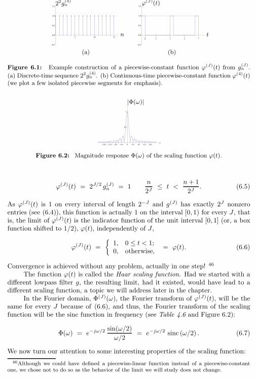
192 Chapter 6. Wavelet Bases, Frames and Transforms on Functions
5 10 15
-0.5
0.0
0.5
1.0
1.5
n
22g(4)n
1
16
1
4
1
2
3
41
-0.5
0.0
0.5
1.0
1.5
t
ϕ(J)(t)
(a) (b)
Figure 6.1: Example construction of a piecewise-constant function ϕ(J)(t) from g(J)n .
(a) Discrete-time sequence 22g(4)n . (b) Continuous-time piecewise-constant function ϕ(4)(t)
(we plot a few isolated piecewise segments for emphasis).
-16Π -12Π -8Π -4Π 0 4Π 8Π 12Π 16Πw
0.5
1
|Φ(ω)|
Figure 6.2: Magnitude response Φ(ω) of the scaling function ϕ(t).
ϕ(J)(t) = 2J/2 g(J)n
= 1n
2J≤ t <
n+ 1
2J. (6.5)
As ϕ(J)(t) is 1 on every interval of length 2−J and g(J) has exactly 2J nonzeroentries (see (6.4)), this function is actually 1 on the interval [0, 1) for every J , thatis, the limit of ϕ(J)(t) is the indicator function of the unit interval [0, 1] (or, a boxfunction shifted to 1/2), ϕ(t), independently of J ,
ϕ(J)(t) =
1, 0 ≤ t < 1;0, otherwise,
= ϕ(t). (6.6)
Convergence is achieved without any problem, actually in one step! 46
The function ϕ(t) is called the Haar scaling function. Had we started with adifferent lowpass filter g, the resulting limit, had it existed, would have lead to adifferent scaling function, a topic we will address later in the chapter.
In the Fourier domain, Φ(J)(ω), the Fourier transform of ϕ(J)(t), will be thesame for every J because of (6.6), and thus, the Fourier transform of the scalingfunction will be the sinc function in frequency (see Table 4.6 and Figure 6.2):
Φ(ω) = e−jω/2sin(ω/2)
ω/2= e−jω/2 sinc (ω/2) . (6.7)
We now turn our attention to some interesting properties of the scaling function:
46Although we could have defined a piecewise-linear function instead of a piecewise-constantone, we chose not to do so as the behavior of the limit we will study does not change.
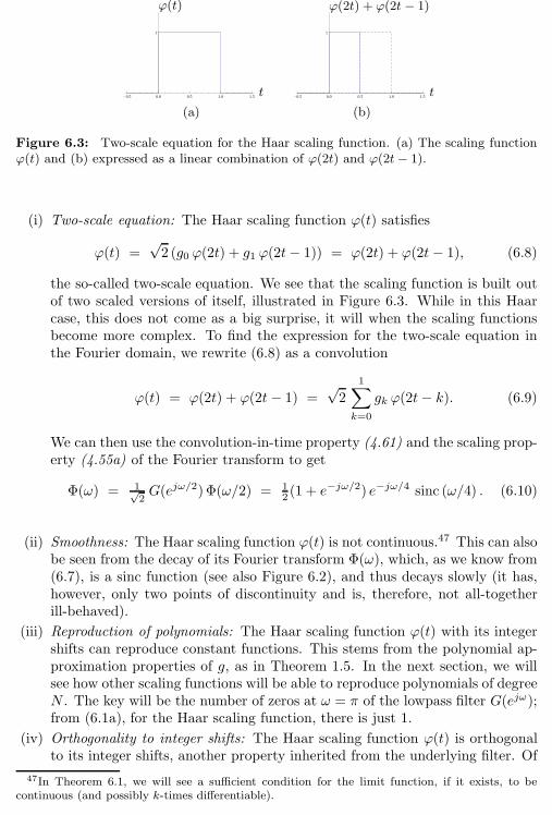
6.1. Introduction 193
-0.5 0.0 0.5 1.0 1.5
1
t
ϕ(t)
-0.5 0.0 0.5 1.0 1.5
1
t
ϕ(2t) + ϕ(2t − 1)
(a) (b)
Figure 6.3: Two-scale equation for the Haar scaling function. (a) The scaling functionϕ(t) and (b) expressed as a linear combination of ϕ(2t) and ϕ(2t− 1).
(i) Two-scale equation: The Haar scaling function ϕ(t) satisfies
ϕ(t) =√2 (g0 ϕ(2t) + g1 ϕ(2t− 1)) = ϕ(2t) + ϕ(2t− 1), (6.8)
the so-called two-scale equation. We see that the scaling function is built outof two scaled versions of itself, illustrated in Figure 6.3. While in this Haarcase, this does not come as a big surprise, it will when the scaling functionsbecome more complex. To find the expression for the two-scale equation inthe Fourier domain, we rewrite (6.8) as a convolution
ϕ(t) = ϕ(2t) + ϕ(2t− 1) =√2
1∑
k=0
gk ϕ(2t− k). (6.9)
We can then use the convolution-in-time property (4.61) and the scaling prop-erty (4.55a) of the Fourier transform to get
Φ(ω) = 1√2G(ejω/2)Φ(ω/2) = 1
2 (1 + e−jω/2) e−jω/4 sinc (ω/4) . (6.10)
(ii) Smoothness: The Haar scaling function ϕ(t) is not continuous.47 This can alsobe seen from the decay of its Fourier transform Φ(ω), which, as we know from(6.7), is a sinc function (see also Figure 6.2), and thus decays slowly (it has,however, only two points of discontinuity and is, therefore, not all-togetherill-behaved).
(iii) Reproduction of polynomials: The Haar scaling function ϕ(t) with its integershifts can reproduce constant functions. This stems from the polynomial ap-proximation properties of g, as in Theorem 1.5. In the next section, we willsee how other scaling functions will be able to reproduce polynomials of degreeN . The key will be the number of zeros at ω = π of the lowpass filter G(ejω);from (6.1a), for the Haar scaling function, there is just 1.
(iv) Orthogonality to integer shifts: The Haar scaling function ϕ(t) is orthogonalto its integer shifts, another property inherited from the underlying filter. Of
47In Theorem 6.1, we will see a sufficient condition for the limit function, if it exists, to becontinuous (and possibly k-times differentiable).
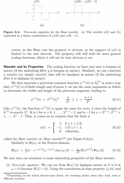
194 Chapter 6. Wavelet Bases, Frames and Transforms on Functions
-0.5 0.5 1.0 1.5
-1.0
-0.5
0.5
1.0
t
ϕ(t)
-0.5 0.5 1.0 1.5
1
t
ϕ(2t) − ϕ(2t − 1)
(a) (b)
Figure 6.4: Two-scale equation for the Haar wavelet. (a) The wavelet ψ(t) and (b)expressed as a linear combination of ϕ(2t) and ϕ(2t− 1).
course, in this Haar case the property is obvious, as the support of ϕ(t) islimited to the unit interval. The property will still hold for more generalscaling functions, albeit it will not be that obvious to see.
Wavelet and its Properties The scaling function we have just seen is lowpass innature (if the underlying filter g is lowpass in nature). Similarly, we can constructa wavelet (or, simply wavelet) that will be bandpass in nature (if the underlyingfilter h is highpass in nature).
We thus associate a piecewise-constant function ψ(J)(t) to h(J)n in such a way
that ψ(J)(t) is of finite length and of norm 1; we use the same arguments as beforeto determine the width and height of the piecewise segments, leading to
ψ(J)(t) = 2J/2 h(J)n
n
2J≤ t <
n+ 1
2J. (6.11)
Like ϕ(J)(t), the function ψ(J)(t) is again the same for every J since the length ofh(J) is exactly 2J . It is 1 for n = 0, 1, . . . , 2J−1−1, and is −1 for n = 2J−1, 2J−1+1, . . . , 2J − 1. Thus, it comes as no surprise that the limit is
ψ(t) =
1, 0 ≤ t < 1/2;−1, 1/2 ≤ t < 1;0, otherwise,
(6.12)
called the Haar wavelet, or, Haar wavelet,48 (see Figure 6.4(a)).Similarly to Φ(ω), in the Fourier-domain,
Ψ(ω) = 12 (1− e
−jω/2) e−jω/4 sinc (ω/4) = 1√2H(ejω/2)Φ(ω/2). (6.13)
We now turn our attention to some interesting properties of the Haar wavelet:
(i) Two-scale equation: We can see from Ψ(ω) its highpass nature as it is 0 atω = 0 (because H(1) = 0). Using the convolution-in-time property (4.61) and
48Depending on the initial discrete-time filters, the resulting limits, when they exist, lead todifferent wavelets.
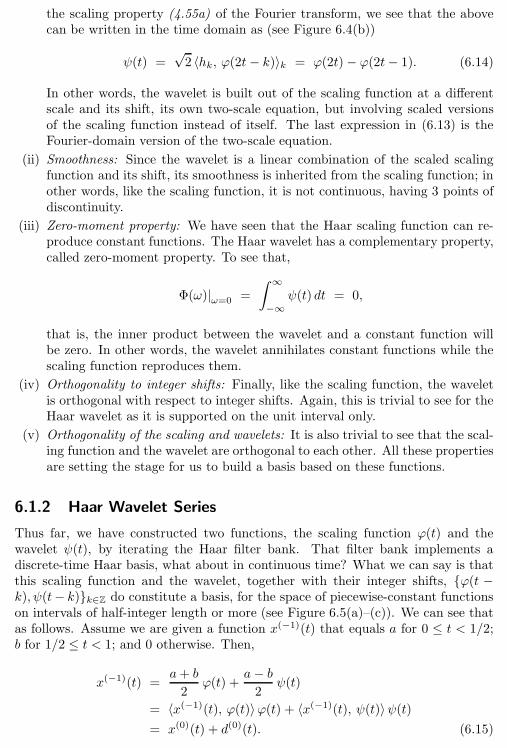
6.1. Introduction 195
the scaling property (4.55a) of the Fourier transform, we see that the abovecan be written in the time domain as (see Figure 6.4(b))
ψ(t) =√2 〈hk, ϕ(2t− k)〉k = ϕ(2t)− ϕ(2t− 1). (6.14)
In other words, the wavelet is built out of the scaling function at a differentscale and its shift, its own two-scale equation, but involving scaled versionsof the scaling function instead of itself. The last expression in (6.13) is theFourier-domain version of the two-scale equation.
(ii) Smoothness: Since the wavelet is a linear combination of the scaled scalingfunction and its shift, its smoothness is inherited from the scaling function; inother words, like the scaling function, it is not continuous, having 3 points ofdiscontinuity.
(iii) Zero-moment property: We have seen that the Haar scaling function can re-produce constant functions. The Haar wavelet has a complementary property,called zero-moment property. To see that,
Φ(ω)|ω=0 =
∫ ∞
−∞ψ(t) dt = 0,
that is, the inner product between the wavelet and a constant function willbe zero. In other words, the wavelet annihilates constant functions while thescaling function reproduces them.
(iv) Orthogonality to integer shifts: Finally, like the scaling function, the waveletis orthogonal with respect to integer shifts. Again, this is trivial to see for theHaar wavelet as it is supported on the unit interval only.
(v) Orthogonality of the scaling and wavelets: It is also trivial to see that the scal-ing function and the wavelet are orthogonal to each other. All these propertiesare setting the stage for us to build a basis based on these functions.
6.1.2 Haar Wavelet Series
Thus far, we have constructed two functions, the scaling function ϕ(t) and thewavelet ψ(t), by iterating the Haar filter bank. That filter bank implements adiscrete-time Haar basis, what about in continuous time? What we can say is thatthis scaling function and the wavelet, together with their integer shifts, ϕ(t −k), ψ(t− k)k∈Z do constitute a basis, for the space of piecewise-constant functionson intervals of half-integer length or more (see Figure 6.5(a)–(c)). We can see thatas follows. Assume we are given a function x(−1)(t) that equals a for 0 ≤ t < 1/2;b for 1/2 ≤ t < 1; and 0 otherwise. Then,
x(−1)(t) =a+ b
2ϕ(t) +
a− b2
ψ(t)
= 〈x(−1)(t), ϕ(t)〉ϕ(t) + 〈x(−1)(t), ψ(t)〉ψ(t)= x(0)(t) + d(0)(t). (6.15)
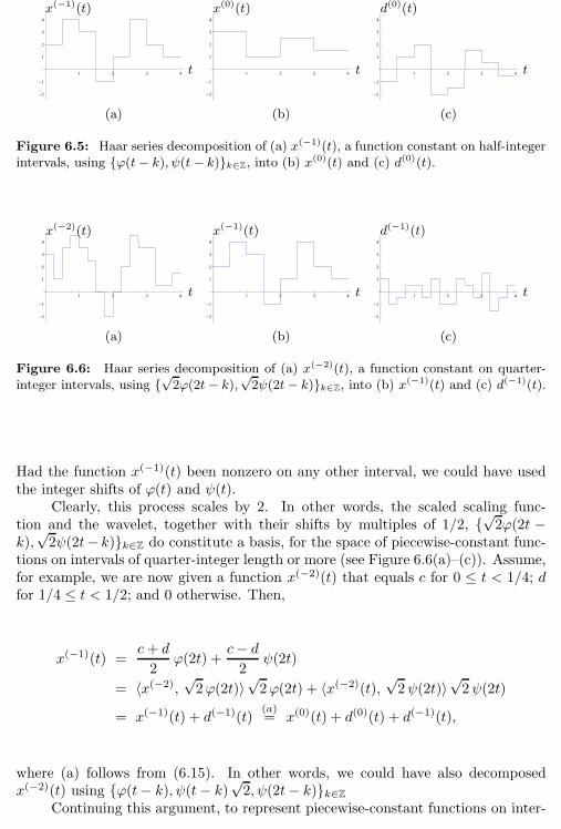
196 Chapter 6. Wavelet Bases, Frames and Transforms on Functions
1 2 3 4
-2
-1
1
2
3
4
t
x(−1)(t)
1 2 3 4
-2
-1
1
2
3
4
t
x(0)(t)
1 2 3 4
-2
-1
1
2
3
4
t
d(0)(t)
(a) (b) (c)
Figure 6.5: Haar series decomposition of (a) x(−1)(t), a function constant on half-integerintervals, using ϕ(t− k), ψ(t− k)k∈Z, into (b) x(0)(t) and (c) d(0)(t).
1 2 3 4
-2
-1
1
2
3
4
t
x(−2)(t)
1 2 3 4
-2
-1
1
2
3
4
t
x(−1)(t)
1 2 3 4
-2
-1
1
2
3
4
t
d(−1)(t)
(a) (b) (c)
Figure 6.6: Haar series decomposition of (a) x(−2)(t), a function constant on quarter-integer intervals, using
√2ϕ(2t− k),
√2ψ(2t− k)k∈Z, into (b) x(−1)(t) and (c) d(−1)(t).
Had the function x(−1)(t) been nonzero on any other interval, we could have usedthe integer shifts of ϕ(t) and ψ(t).
Clearly, this process scales by 2. In other words, the scaled scaling func-tion and the wavelet, together with their shifts by multiples of 1/2,
√2ϕ(2t −
k),√2ψ(2t− k)k∈Z do constitute a basis, for the space of piecewise-constant func-
tions on intervals of quarter-integer length or more (see Figure 6.6(a)–(c)). Assume,for example, we are now given a function x(−2)(t) that equals c for 0 ≤ t < 1/4; dfor 1/4 ≤ t < 1/2; and 0 otherwise. Then,
x(−1)(t) =c+ d
2ϕ(2t) +
c− d2
ψ(2t)
= 〈x(−2),√2ϕ(2t)〉
√2ϕ(2t) + 〈x(−2)(t),
√2ψ(2t)〉
√2ψ(2t)
= x(−1)(t) + d(−1)(t)(a)= x(0)(t) + d(0)(t) + d(−1)(t),
where (a) follows from (6.15). In other words, we could have also decomposedx(−2)(t) using ϕ(t− k), ψ(t− k)
√2, ψ(2t− k)k∈Z
Continuing this argument, to represent piecewise-constant functions on inter-
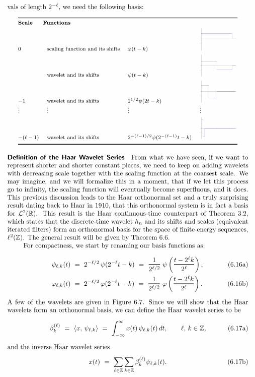
6.1. Introduction 197
vals of length 2−ℓ, we need the following basis:
Scale Functions
0 scaling function and its shifts ϕ(t − k)
-
wavelet and its shifts ψ(t − k)-
−1 wavelet and its shifts 21/2ψ(2t − k)-
......
......
−(ℓ− 1) wavelet and its shifts 2−(ℓ−1)/2ψ(2−(ℓ−1)t− k)-
Definition of the Haar Wavelet Series From what we have seen, if we want torepresent shorter and shorter constant pieces, we need to keep on adding waveletswith decreasing scale together with the scaling function at the coarsest scale. Wemay imagine, and we will formalize this in a moment, that if we let this processgo to infinity, the scaling function will eventually become superfluous, and it does.This previous discussion leads to the Haar orthonormal set and a truly surprisingresult dating back to Haar in 1910, that this orthonormal system is in fact a basisfor L2(R). This result is the Haar continuous-time counterpart of Theorem 3.2,which states that the discrete-time wavelet hn and its shifts and scales (equivalentiterated filters) form an orthonormal basis for the space of finite-energy sequences,ℓ2(Z). The general result will be given by Theorem 6.6.
For compactness, we start by renaming our basis functions as:
ψℓ,k(t) = 2−ℓ/2 ψ(2−ℓt− k) =1
2ℓ/2ψ
(t− 2ℓk
2ℓ
), (6.16a)
ϕℓ,k(t) = 2−ℓ/2 ϕ(2−ℓt− k) =1
2ℓ/2ϕ
(t− 2ℓk
2ℓ
). (6.16b)
A few of the wavelets are given in Figure 6.7. Since we will show that the Haarwavelets form an orthonormal basis, we can define the Haar wavelet series to be
β(ℓ)k
= 〈x, ψℓ,k〉 =
∫ ∞
−∞x(t)ψℓ,k(t) dt, ℓ, k ∈ Z, (6.17a)
and the inverse Haar wavelet series
x(t) =∑
ℓ∈Z
∑
k∈Z
β(ℓ)kψℓ,k(t). (6.17b)
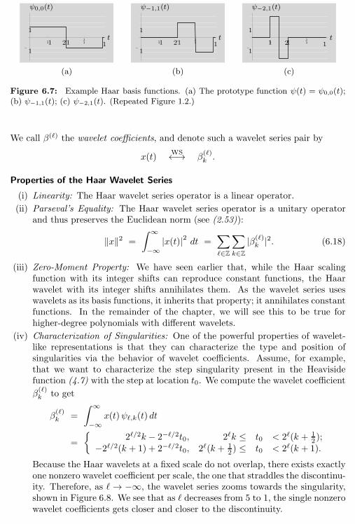
198 Chapter 6. Wavelet Bases, Frames and Transforms on Functions
434
-
t
ψ0,0(t)
2
1
1111 4
34
-
t
ψ−1,1(t)
2
1
1111 4
34
-
t
ψ−2,1(t)
1
1111 2
(a) (b) (c)
Figure 6.7: Example Haar basis functions. (a) The prototype function ψ(t) = ψ0,0(t);(b) ψ−1,1(t); (c) ψ−2,1(t). (Repeated Figure 1.2.)
We call β(ℓ) the wavelet coefficients, and denote such a wavelet series pair by
x(t)WS←→ β
(ℓ)k.
Properties of the Haar Wavelet Series
(i) Linearity: The Haar wavelet series operator is a linear operator.
(ii) Parseval’s Equality: The Haar wavelet series operator is a unitary operatorand thus preserves the Euclidean norm (see (2.53)):
‖x‖2 =
∫ ∞
−∞|x(t)|2 dt =
∑
ℓ∈Z
∑
k∈Z
|β(ℓ)k|2. (6.18)
(iii) Zero-Moment Property: We have seen earlier that, while the Haar scalingfunction with its integer shifts can reproduce constant functions, the Haarwavelet with its integer shifts annihilates them. As the wavelet series useswavelets as its basis functions, it inherits that property; it annihilates constantfunctions. In the remainder of the chapter, we will see this to be true forhigher-degree polynomials with different wavelets.
(iv) Characterization of Singularities: One of the powerful properties of wavelet-like representations is that they can characterize the type and position ofsingularities via the behavior of wavelet coefficients. Assume, for example,that we want to characterize the step singularity present in the Heavisidefunction (4.7) with the step at location t0. We compute the wavelet coefficient
β(ℓ)k
to get
β(ℓ)k
=
∫ ∞
−∞x(t)ψℓ,k(t) dt
=
2ℓ/2k − 2−ℓ/2t0, 2ℓk ≤ t0 < 2ℓ(k + 1
2 );
−2ℓ/2(k + 1) + 2−ℓ/2t0, 2ℓ(k + 12 ) ≤ t0 < 2ℓ(k + 1).
Because the Haar wavelets at a fixed scale do not overlap, there exists exactlyone nonzero wavelet coefficient per scale, the one that straddles the discontinu-ity. Therefore, as ℓ → −∞, the wavelet series zooms towards the singularity,shown in Figure 6.8. We see that as ℓ decreases from 5 to 1, the single nonzerowavelet coefficients gets closer and closer to the discontinuity.
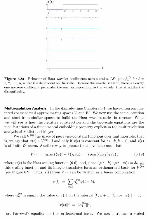
6.1. Introduction 199
0 5 10 15 20 25 30
1
x(t)
t
0
5
4
3
2
1
k
ℓ
Figure 6.8: Behavior of Haar wavelet coefficients across scales. We plot β(ℓ)k for ℓ =
1, 2, . . . , 5, where k is dependent on the scale. Because the wavelet is Haar, there is exactlyone nonzero coefficient per scale, the one corresponding to the wavelet that straddles thediscontinuity.
Multiresolution Analysis In the discrete-time Chapters 1-4, we have often encoun-tered coarse/detail approximating spaces V andW . We now use the same intuitionand start from similar spaces to build the Haar wavelet series in reverse. Whatwe will see is how the iterative construction and the two-scale equations are themanifestations of a fundamental embedding property explicit in the multiresolutionanalysis of Mallat and Meyer.
We call V (0) the space of piecewise-constant functions over unit intervals, thatis, we say that x(t) ∈ V (0), if and only if x(t) is constant for t ∈ [k, k+ 1), and x(t)is of finite L2 norm. Another way to phrase the above is to note that
V (0) = span (ϕ(t− k)k∈Z) = span (ϕ0,kk∈Z) , (6.19)
where ϕ(t) is the Haar scaling function (6.6), and, since 〈ϕ(t−k), ϕ(t−m)〉 = δk−m,this scaling function and its integer translates form an orthonormal basis for V (0)
(see Figure 6.9). Thus, x(t) from V (0) can be written as a linear combination
x(t) =∑
k∈Z
α(0)kϕ(t− k),
where α(0)k
is simply the value of x(t) on the interval [k, k + 1). Since ‖ϕ(t‖ = 1,
‖x(t)‖2 = ‖α(0)k‖2,
or, Parseval’s equality for this orthonormal basis. We now introduce a scaled
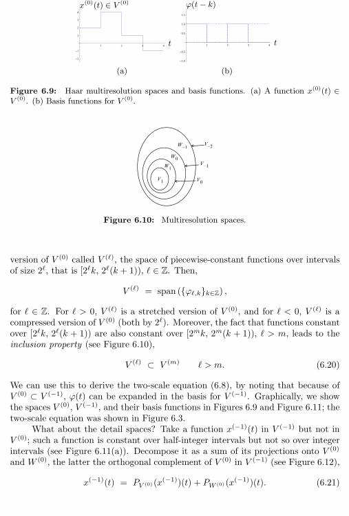
200 Chapter 6. Wavelet Bases, Frames and Transforms on Functions
1 2 3 4
-2
-1
1
2
3
4
t
x(0)(t) ∈ V (0)
1 2 3 4
-1.0
-0.5
0.5
1.0
1.5
t
ϕ(t− k)
(a) (b)
Figure 6.9: Haar multiresolution spaces and basis functions. (a) A function x(0)(t) ∈V (0). (b) Basis functions for V (0).
Figure 6.10: Multiresolution spaces.
version of V (0) called V (ℓ), the space of piecewise-constant functions over intervalsof size 2ℓ, that is [2ℓk, 2ℓ(k + 1)), ℓ ∈ Z. Then,
V (ℓ) = span (ϕℓ,kk∈Z) ,
for ℓ ∈ Z. For ℓ > 0, V (ℓ) is a stretched version of V (0), and for ℓ < 0, V (ℓ) is acompressed version of V (0) (both by 2ℓ). Moreover, the fact that functions constantover [2ℓk, 2ℓ(k + 1)) are also constant over [2mk, 2m(k + 1)), ℓ > m, leads to theinclusion property (see Figure 6.10),
V (ℓ) ⊂ V (m) ℓ > m. (6.20)
We can use this to derive the two-scale equation (6.8), by noting that because ofV (0) ⊂ V (−1), ϕ(t) can be expanded in the basis for V (−1). Graphically, we showthe spaces V (0), V (−1), and their basis functions in Figures 6.9 and Figure 6.11; thetwo-scale equation was shown in Figure 6.3.
What about the detail spaces? Take a function x(−1)(t) in V (−1) but not inV (0); such a function is constant over half-integer intervals but not so over integerintervals (see Figure 6.11(a)). Decompose it as a sum of its projections onto V (0)
and W (0), the latter the orthogonal complement of V (0) in V (−1) (see Figure 6.12),
x(−1)(t) = PV
(0)(x(−1))(t) + PW
(0)(x(−1))(t). (6.21)
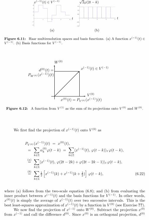
6.1. Introduction 201
1 2 3 4
-2
-1
1
2
3
4
t
x(−1)(t) ∈ V (−1)
1 2 3 4
-1.0
-0.5
0.5
1.0
1.5
t
√2ϕ(2t− k)
(a) (b)
Figure 6.11: Haar multiresolution spaces and basis functions. (a) A function x(−1)(t) ∈V (−1). (b) Basis functions for V (−1).
d(0)(t) =PW
(0)(x(−1))(t)
x(0)(t) = PV
(0)(x(−1))(t)
x(−1)(t) ∈ V (−1)
V (0)
W (0)
Figure 6.12: A function from V (1) as the sum of its projections onto V (0) and W (0).
We first find the projection of x(−1)(t) onto V (0) as
PV
(0)(x(−1))(t) = x(0)(t),
=∑
k∈Z
α(0)kϕ(t− k) =
∑
k∈Z
〈x(−1)(t), ϕ(t− k)〉t ϕ(t− k),
(a)=∑
k∈Z
〈x(−1)(t), ϕ(2t− 2k) + ϕ(2t− 2k − 1)〉t ϕ(t− k),
(b)=∑
k∈Z
12
[x(−1)(k) + x(−1)(k + 1
2 )]ϕ(t− k), (6.22)
where (a) follows from the two-scale equation (6.8); and (b) from evaluating theinner product between x(−1)(t) and the basis functions for V (−1). In other words,x(0)(t) is simply the average of x(−1)(t) over two successive intervals. This is thebest least-squares approximation of x(−1)(t) by a function in V (0) (see Exercise ??).
We now find the projection of x(−1) onto W (0). Subtract the projection x(0)
from x(−1) and call the difference d(0). Since x(0) is an orthogonal projection, d(0)
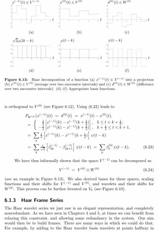
202 Chapter 6. Wavelet Bases, Frames and Transforms on Functions
1 2 3 4
-2
-1
1
2
3
4
t
x(−1)(t) ∈ V (−1)
1 2 3 4
-2
-1
1
2
3
4
t
x(0)(t) ∈ V (0)
1 2 3 4
-2
-1
1
2
3
4
t
d(0)(t) ∈ W (0)
(a) (b) (c)
1 2 3 4
-1.0
-0.5
0.5
1.0
1.5
t
√2ϕ(2t− k)
1 2 3 4
-1.0
-0.5
0.5
1.0
1.5
t
ϕ(t− k)
1 2 3 4
-1.0
-0.5
0.5
1.0
1.5
t
ψ(t− k)
(d) (e) (f)
Figure 6.13: Haar decomposition of a function (a) x(−1)(t) ∈ V (−1) into a projection(b) x(0)(t) ∈ V (0) (average over two successive intervals) and (c) d(0)(t) ∈W (0) (differenceover two successive intervals). (d)–(f) Appropriate basis functions.
is orthogonal to V (0) (see Figure 6.12). Using (6.22) leads to
PW
(0)(x(−1))(t) = d(0)(t) = x(−1)(t)− x(0)(t),
=
12
[x(−1)(k)− x(−1)(k + 1
2 )], k ≤ t < k + 1
2 ;
− 12
[x(−1)(k)− x(−1)(k + 1
2 )], k + 1
2 ≤ t < k + 1,
=∑
k
12
[x(−1)(k)− x(−1)(k + 1
2 )]ψ(t− k)
=∑
k
1√2
[β(−1)2k − β(−1)
2k+1
]ψ(t− k) =
∑
k
β(0)kψ(t− k). (6.23)
We have thus informally shown that the space V (−1) can be decomposed as
V (−1) = V (0) ⊕W (0) (6.24)
(see an example in Figure 6.13). We also derived bases for these spaces, scalingfunctions and their shifts for V (−1) and V (0), and wavelets and their shifts forW (0). This process can be further iterated on V0 (see Figure 6.10).
6.1.3 Haar Frame Series
The Haar wavelet series we just saw is an elegant representation, and completelynonredundant. As we have seen in Chapters 4 and 5, at times we can benefit fromrelaxing this constraint, and allowing some redundancy in the system. Our aimwould then be to build frames. There are many ways in which we could do that.For example, by adding to the Haar wavelet basis wavelets at points halfway in
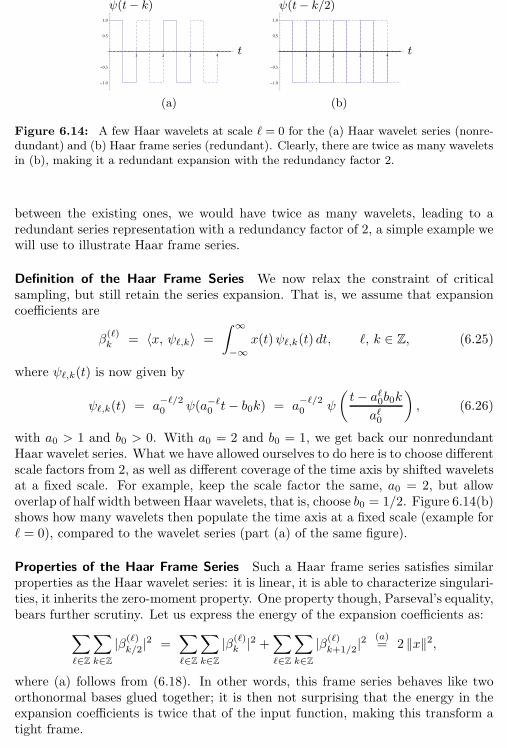
6.1. Introduction 203
1 2 3 4
-1.0
-0.5
0.5
1.0
t
ψ(t− k)
1 2 3 4
-1.0
-0.5
0.5
1.0
t
ψ(t− k/2)
(a) (b)
Figure 6.14: A few Haar wavelets at scale ℓ = 0 for the (a) Haar wavelet series (nonre-dundant) and (b) Haar frame series (redundant). Clearly, there are twice as many waveletsin (b), making it a redundant expansion with the redundancy factor 2.
between the existing ones, we would have twice as many wavelets, leading to aredundant series representation with a redundancy factor of 2, a simple example wewill use to illustrate Haar frame series.
Definition of the Haar Frame Series We now relax the constraint of criticalsampling, but still retain the series expansion. That is, we assume that expansioncoefficients are
β(ℓ)k
= 〈x, ψℓ,k〉 =
∫ ∞
−∞x(t)ψℓ,k(t) dt, ℓ, k ∈ Z, (6.25)
where ψℓ,k(t) is now given by
ψℓ,k(t) = a−ℓ/20 ψ(a−ℓ0 t− b0k) = a
−ℓ/20 ψ
(t− aℓ0b0k
aℓ0
), (6.26)
with a0 > 1 and b0 > 0. With a0 = 2 and b0 = 1, we get back our nonredundantHaar wavelet series. What we have allowed ourselves to do here is to choose differentscale factors from 2, as well as different coverage of the time axis by shifted waveletsat a fixed scale. For example, keep the scale factor the same, a0 = 2, but allowoverlap of half width between Haar wavelets, that is, choose b0 = 1/2. Figure 6.14(b)shows how many wavelets then populate the time axis at a fixed scale (example forℓ = 0), compared to the wavelet series (part (a) of the same figure).
Properties of the Haar Frame Series Such a Haar frame series satisfies similarproperties as the Haar wavelet series: it is linear, it is able to characterize singulari-ties, it inherits the zero-moment property. One property though, Parseval’s equality,bears further scrutiny. Let us express the energy of the expansion coefficients as:
∑
ℓ∈Z
∑
k∈Z
|β(ℓ)k/2|2 =
∑
ℓ∈Z
∑
k∈Z
|β(ℓ)k|2 +
∑
ℓ∈Z
∑
k∈Z
|β(ℓ)k+1/2|2
(a)= 2 ‖x‖2,
where (a) follows from (6.18). In other words, this frame series behaves like twoorthonormal bases glued together; it is then not surprising that the energy in theexpansion coefficients is twice that of the input function, making this transform atight frame.
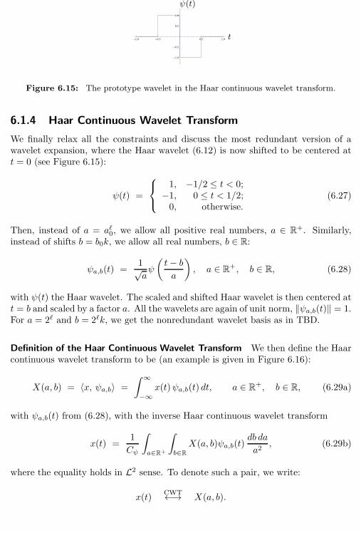
204 Chapter 6. Wavelet Bases, Frames and Transforms on Functions
-1.0 -0.5 0.5 1.0
-1.0
-0.5
0.5
1.0
t
ψ(t)
Figure 6.15: The prototype wavelet in the Haar continuous wavelet transform.
6.1.4 Haar Continuous Wavelet Transform
We finally relax all the constraints and discuss the most redundant version of awavelet expansion, where the Haar wavelet (6.12) is now shifted to be centered att = 0 (see Figure 6.15):
ψ(t) =
1, −1/2 ≤ t < 0;−1, 0 ≤ t < 1/2;0, otherwise.
(6.27)
Then, instead of a = aℓ0, we allow all positive real numbers, a ∈ R+. Similarly,instead of shifts b = b0k, we allow all real numbers, b ∈ R:
ψa,b(t) =1√aψ
(t− ba
), a ∈ R
+, b ∈ R, (6.28)
with ψ(t) the Haar wavelet. The scaled and shifted Haar wavelet is then centered att = b and scaled by a factor a. All the wavelets are again of unit norm, ‖ψa,b(t)‖ = 1.For a = 2ℓ and b = 2ℓk, we get the nonredundant wavelet basis as in TBD.
Definition of the Haar Continuous Wavelet Transform We then define the Haarcontinuous wavelet transform to be (an example is given in Figure 6.16):
X(a, b) = 〈x, ψa,b〉 =
∫ ∞
−∞x(t)ψa,b(t) dt, a ∈ R
+, b ∈ R, (6.29a)
with ψa,b(t) from (6.28), with the inverse Haar continuous wavelet transform
x(t) =1
Cψ
∫
a∈R+
∫
b∈R
X(a, b)ψa,b(t)db da
a2, (6.29b)
where the equality holds in L2 sense. To denote such a pair, we write:
x(t)CWT←→ X(a, b).
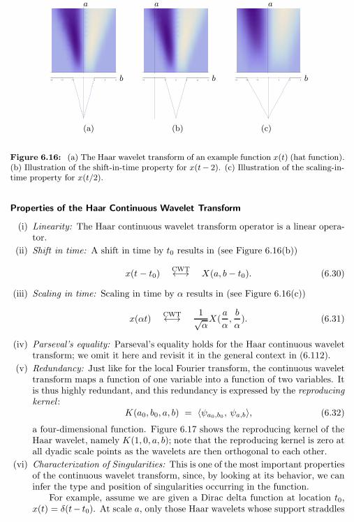
6.1. Introduction 205
a a a
-3 -2 -1 1 2 3 b -1 1 2 3 4 5 b -3 -2 -1 1 2 3 b
(a) (b) (c)
Figure 6.16: (a) The Haar wavelet transform of an example function x(t) (hat function).(b) Illustration of the shift-in-time property for x(t− 2). (c) Illustration of the scaling-in-time property for x(t/2).
Properties of the Haar Continuous Wavelet Transform
(i) Linearity: The Haar continuous wavelet transform operator is a linear opera-tor.
(ii) Shift in time: A shift in time by t0 results in (see Figure 6.16(b))
x(t − t0) CWT←→ X(a, b− t0). (6.30)
(iii) Scaling in time: Scaling in time by α results in (see Figure 6.16(c))
x(αt)CWT←→ 1√
αX(
a
α,b
α). (6.31)
(iv) Parseval’s equality: Parseval’s equality holds for the Haar continuous wavelettransform; we omit it here and revisit it in the general context in (6.112).
(v) Redundancy: Just like for the local Fourier transform, the continuous wavelettransform maps a function of one variable into a function of two variables. Itis thus highly redundant, and this redundancy is expressed by the reproducingkernel :
K(a0, b0, a, b) = 〈ψa0,b0 , ψa,b〉, (6.32)
a four-dimensional function. Figure 6.17 shows the reproducing kernel of theHaar wavelet, namely K(1, 0, a, b); note that the reproducing kernel is zero atall dyadic scale points as the wavelets are then orthogonal to each other.
(vi) Characterization of Singularities: This is one of the most important propertiesof the continuous wavelet transform, since, by looking at its behavior, we caninfer the type and position of singularities occurring in the function.
For example, assume we are given a Dirac delta function at location t0,x(t) = δ(t− t0). At scale a, only those Haar wavelets whose support straddles
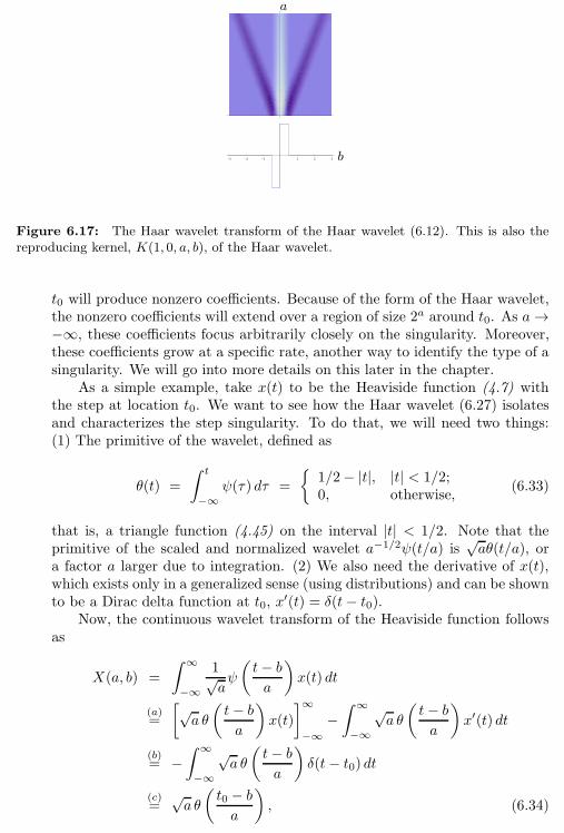
206 Chapter 6. Wavelet Bases, Frames and Transforms on Functions
a
-3 -2 -1 1 2 3 b
Figure 6.17: The Haar wavelet transform of the Haar wavelet (6.12). This is also thereproducing kernel, K(1, 0, a, b), of the Haar wavelet.
t0 will produce nonzero coefficients. Because of the form of the Haar wavelet,the nonzero coefficients will extend over a region of size 2a around t0. As a→−∞, these coefficients focus arbitrarily closely on the singularity. Moreover,these coefficients grow at a specific rate, another way to identify the type of asingularity. We will go into more details on this later in the chapter.
As a simple example, take x(t) to be the Heaviside function (4.7) withthe step at location t0. We want to see how the Haar wavelet (6.27) isolatesand characterizes the step singularity. To do that, we will need two things:(1) The primitive of the wavelet, defined as
θ(t) =
∫t
−∞ψ(τ) dτ =
1/2− |t|, |t| < 1/2;0, otherwise,
(6.33)
that is, a triangle function (4.45) on the interval |t| < 1/2. Note that theprimitive of the scaled and normalized wavelet a−1/2ψ(t/a) is
√aθ(t/a), or
a factor a larger due to integration. (2) We also need the derivative of x(t),which exists only in a generalized sense (using distributions) and can be shownto be a Dirac delta function at t0, x
′(t) = δ(t− t0).Now, the continuous wavelet transform of the Heaviside function follows
as
X(a, b) =
∫ ∞
−∞
1√aψ
(t− ba
)x(t) dt
(a)=
[√a θ
(t− ba
)x(t)
]∞
−∞−∫ ∞
−∞
√a θ
(t− ba
)x′(t) dt
(b)= −
∫ ∞
−∞
√a θ
(t− ba
)δ(t− t0) dt
(c)=√a θ
(t0 − ba
), (6.34)
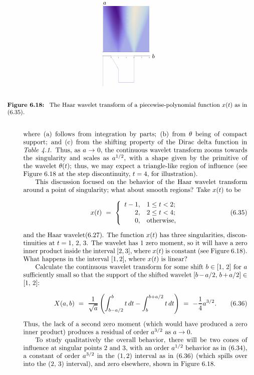
6.1. Introduction 207
a
1 2 3 4 5 6 b
Figure 6.18: The Haar wavelet transform of a piecewise-polynomial function x(t) as in(6.35).
where (a) follows from integration by parts; (b) from θ being of compactsupport; and (c) from the shifting property of the Dirac delta function inTable 4.1. Thus, as a → 0, the continuous wavelet transform zooms towardsthe singularity and scales as a1/2, with a shape given by the primitive ofthe wavelet θ(t); thus, we may expect a triangle-like region of influence (seeFigure 6.18 at the step discontinuity, t = 4, for illustration).
This discussion focused on the behavior of the Haar wavelet transformaround a point of singularity; what about smooth regions? Take x(t) to be
x(t) =
t− 1, 1 ≤ t < 2;2, 2 ≤ t < 4;0, otherwise,
(6.35)
and the Haar wavelet(6.27). The function x(t) has three singularities, discon-tinuities at t = 1, 2, 3. The wavelet has 1 zero moment, so it will have a zeroinner product inside the interval [2, 3], where x(t) is constant (see Figure 6.18).What happens in the interval [1, 2], where x(t) is linear?
Calculate the continuous wavelet transform for some shift b ∈ [1, 2] for asufficiently small so that the support of the shifted wavelet [b−a/2, b+a/2] ∈[1, 2]:
X(a, b) =1√a
(∫b
b−a/2t dt−
∫b+a/2
b
t dt
)= −1
4a3/2. (6.36)
Thus, the lack of a second zero moment (which would have produced a zeroinner product) produces a residual of order a3/2 as a→ 0.
To study qualitatively the overall behavior, there will be two cones ofinfluence at singular points 2 and 3, with an order a1/2 behavior as in (6.34),a constant of order a3/2 in the (1, 2) interval as in (6.36) (which spills overinto the (2, 3) interval), and zero elsewhere, shown in Figure 6.18.
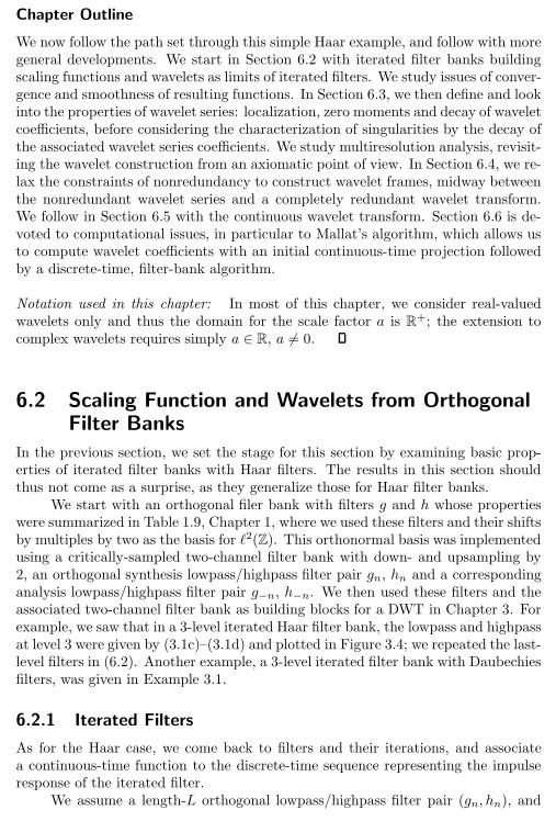
208 Chapter 6. Wavelet Bases, Frames and Transforms on Functions
Chapter Outline
We now follow the path set through this simple Haar example, and follow with moregeneral developments. We start in Section 6.2 with iterated filter banks buildingscaling functions and wavelets as limits of iterated filters. We study issues of conver-gence and smoothness of resulting functions. In Section 6.3, we then define and lookinto the properties of wavelet series: localization, zero moments and decay of waveletcoefficients, before considering the characterization of singularities by the decay ofthe associated wavelet series coefficients. We study multiresolution analysis, revisit-ing the wavelet construction from an axiomatic point of view. In Section 6.4, we re-lax the constraints of nonredundancy to construct wavelet frames, midway betweenthe nonredundant wavelet series and a completely redundant wavelet transform.We follow in Section 6.5 with the continuous wavelet transform. Section 6.6 is de-voted to computational issues, in particular to Mallat’s algorithm, which allows usto compute wavelet coefficients with an initial continuous-time projection followedby a discrete-time, filter-bank algorithm.
Notation used in this chapter: In most of this chapter, we consider real-valuedwavelets only and thus the domain for the scale factor a is R+; the extension tocomplex wavelets requires simply a ∈ R, a 6= 0.
6.2 Scaling Function and Wavelets from OrthogonalFilter Banks
In the previous section, we set the stage for this section by examining basic prop-erties of iterated filter banks with Haar filters. The results in this section shouldthus not come as a surprise, as they generalize those for Haar filter banks.
We start with an orthogonal filer bank with filters g and h whose propertieswere summarized in Table 1.9, Chapter 1, where we used these filters and their shiftsby multiples by two as the basis for ℓ2(Z). This orthonormal basis was implementedusing a critically-sampled two-channel filter bank with down- and upsampling by2, an orthogonal synthesis lowpass/highpass filter pair gn, hn and a correspondinganalysis lowpass/highpass filter pair g−n, h−n. We then used these filters and theassociated two-channel filter bank as building blocks for a DWT in Chapter 3. Forexample, we saw that in a 3-level iterated Haar filter bank, the lowpass and highpassat level 3 were given by (3.1c)–(3.1d) and plotted in Figure 3.4; we repeated the last-level filters in (6.2). Another example, a 3-level iterated filter bank with Daubechiesfilters, was given in Example 3.1.
6.2.1 Iterated Filters
As for the Haar case, we come back to filters and their iterations, and associatea continuous-time function to the discrete-time sequence representing the impulseresponse of the iterated filter.
We assume a length-L orthogonal lowpass/highpass filter pair (gn, hn), and
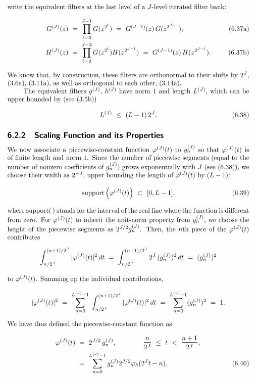
6.2. Scaling Function and Wavelets from Orthogonal Filter Banks 209
write the equivalent filters at the last level of a J-level iterated filter bank:
G(J)(z) =
J−1∏
ℓ=0
G(z2ℓ
) = G(J−1)(z)G(z2J−1
), (6.37a)
H(J)(z) =
J−2∏
ℓ=0
G(z2ℓ
)H(z2J−1
) = G(J−1)(z)H(z2J−1
). (6.37b)
We know that, by construction, these filters are orthonormal to their shifts by 2J ,(3.6a), (3.11a), as well as orthogonal to each other, (3.14a).
The equivalent filters g(J), h(J) have norm 1 and length L(J), which can beupper bounded by (see (3.5b))
L(J) ≤ (L− 1) 2J . (6.38)
6.2.2 Scaling Function and its Properties
We now associate a piecewise-constant function ϕ(J)(t) to g(J)n so that ϕ(J)(t) is
of finite length and norm 1. Since the number of piecewise segments (equal to the
number of nonzero coefficients of g(J)n ) grows exponentially with J (see (6.38)), we
choose their width as 2−J , upper bounding the length of ϕ(J)(t) by (L − 1):
support(ϕ(J)(t)
)⊂ [0, L− 1], (6.39)
where support( ) stands for the interval of the real line where the function is different
from zero. For ϕ(J)(t) to inherit the unit-norm property from g(J)n , we choose the
height of the piecewise segments as 2J/2g(J)n . Then, the nth piece of the ϕ(J)(t)
contributes
∫ (n+1)/2J
n/2J|ϕ(J)(t)|2 dt =
∫ (n+1)/2J
n/2J2J (g(J)
n)2 dt = (g(J)
n)2
to ϕ(J)(t). Summing up the individual contributions,
|ϕ(J)(t)|2 =
L(J)−1∑
n=0
∫ (n+1)/2J
n/2J|ϕ(J)(t)|2 dt =
L(J)−1∑
n=0
(g(J)n
)2 = 1.
We have thus defined the piecewise-constant function as
ϕ(J)(t) = 2J/2 g(J)n,
n
2J≤ t <
n+ 1
2J,
=
L(J)−1∑
n=0
g(J)n
2J/2ϕh(2J t− n), (6.40)
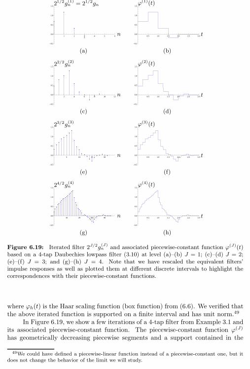
210 Chapter 6. Wavelet Bases, Frames and Transforms on Functions
1 2 3 4 5 6
-0.5
0.0
0.5
1.0
1.5
n
21/2g(1)n = 21/2gn
0.5 1.0 1.5 2.0 2.5 3.0
-0.5
0.0
0.5
1.0
1.5
t
ϕ(1)(t)
(a) (b)
2 4 6 8 10 12
-0.5
0.0
0.5
1.0
1.5
n
22/2g(2)n
0.5 1.0 1.5 2.0 2.5 3.0
-0.5
0.0
0.5
1.0
1.5
t
ϕ(2)(t)
(c) (d)
5 10 15 20
-0.5
0.0
0.5
1.0
1.5
n
23/2g(3)n
0.5 1.0 1.5 2.0 2.5 3.0
-0.5
0.0
0.5
1.0
1.5
t
ϕ(3)(t)
(e) (f)
10 20 30 40
-0.5
0.0
0.5
1.0
1.5
n
24/2g(4)n
0.5 1.0 1.5 2.0 2.5 3.0
-0.5
0.0
0.5
1.0
1.5
t
ϕ(4)(t)
(g) (h)
Figure 6.19: Iterated filter 2J/2g(J)n and associated piecewise-constant function ϕ(J)(t)
based on a 4-tap Daubechies lowpass filter (3.10) at level (a)–(b) J = 1; (c)–(d) J = 2;(e)–(f) J = 3; and (g)–(h) J = 4. Note that we have rescaled the equivalent filters’impulse responses as well as plotted them at different discrete intervals to highlight thecorrespondences with their piecewise-constant functions.
where ϕh(t) is the Haar scaling function (box function) from (6.6). We verified thatthe above iterated function is supported on a finite interval and has unit norm.49
In Figure 6.19, we show a few iterations of a 4-tap filter from Example 3.1 andits associated piecewise-constant function. The piecewise-constant function ϕ(J)
has geometrically decreasing piecewise segments and a support contained in the
49We could have defined a piecewise-linear function instead of a piecewise-constant one, but itdoes not change the behavior of the limit we will study.
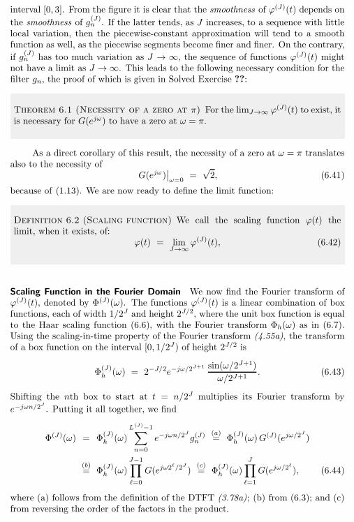
6.2. Scaling Function and Wavelets from Orthogonal Filter Banks 211
interval [0, 3]. From the figure it is clear that the smoothness of ϕ(J)(t) depends on
the smoothness of g(J)n . If the latter tends, as J increases, to a sequence with little
local variation, then the piecewise-constant approximation will tend to a smoothfunction as well, as the piecewise segments become finer and finer. On the contrary,
if g(J)n has too much variation as J → ∞, the sequence of functions ϕ(J)(t) might
not have a limit as J →∞. This leads to the following necessary condition for thefilter gn, the proof of which is given in Solved Exercise ??:
Theorem 6.1 (Necessity of a zero at π) For the limJ→∞ ϕ(J)(t) to exist, itis necessary for G(ejω) to have a zero at ω = π.
As a direct corollary of this result, the necessity of a zero at ω = π translatesalso to the necessity of
G(ejω)∣∣ω=0
=√2, (6.41)
because of (1.13). We are now ready to define the limit function:
Definition 6.2 (Scaling function) We call the scaling function ϕ(t) thelimit, when it exists, of:
ϕ(t) = limJ→∞
ϕ(J)(t), (6.42)
Scaling Function in the Fourier Domain We now find the Fourier transform ofϕ(J)(t), denoted by Φ(J)(ω). The functions ϕ(J)(t) is a linear combination of boxfunctions, each of width 1/2J and height 2J/2, where the unit box function is equalto the Haar scaling function (6.6), with the Fourier transform Φh(ω) as in (6.7).Using the scaling-in-time property of the Fourier transform (4.55a), the transformof a box function on the interval [0, 1/2J) of height 2J/2 is
Φ(J)h
(ω) = 2−J/2e−jω/2J+1 sin(ω/2J+1)
ω/2J+1. (6.43)
Shifting the nth box to start at t = n/2J multiplies its Fourier transform by
e−jωn/2J
. Putting it all together, we find
Φ(J)(ω) = Φ(J)h
(ω)L
(J)−1∑
n=0
e−jωn/2J
g(J)n
(a)= Φ
(J)h
(ω)G(J)(ejω/2J
)
(b)= Φ
(J)h
(ω)
J−1∏
ℓ=0
G(ejω2ℓ/2J )
(c)= Φ
(J)h
(ω)
J∏
ℓ=1
G(ejω/2ℓ
), (6.44)
where (a) follows from the definition of the DTFT (3.78a); (b) from (6.3); and (c)from reversing the order of the factors in the product.
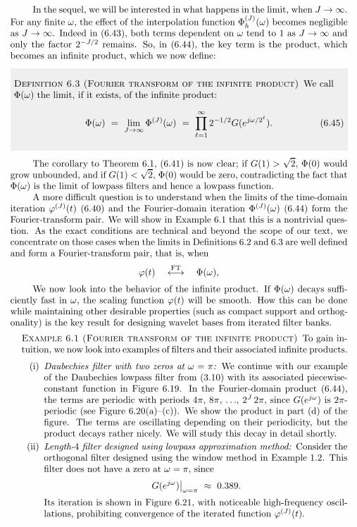
212 Chapter 6. Wavelet Bases, Frames and Transforms on Functions
In the sequel, we will be interested in what happens in the limit, when J →∞.
For any finite ω, the effect of the interpolation function Φ(J)h
(ω) becomes negligibleas J → ∞. Indeed in (6.43), both terms dependent on ω tend to 1 as J → ∞ andonly the factor 2−J/2 remains. So, in (6.44), the key term is the product, whichbecomes an infinite product, which we now define:
Definition 6.3 (Fourier transform of the infinite product) We callΦ(ω) the limit, if it exists, of the infinite product:
Φ(ω) = limJ→∞
Φ(J)(ω) =
∞∏
ℓ=1
2−1/2G(ejω/2ℓ
). (6.45)
The corollary to Theorem 6.1, (6.41) is now clear; if G(1) >√2, Φ(0) would
grow unbounded, and if G(1) <√2, Φ(0) would be zero, contradicting the fact that
Φ(ω) is the limit of lowpass filters and hence a lowpass function.A more difficult question is to understand when the limits of the time-domain
iteration ϕ(J)(t) (6.40) and the Fourier-domain iteration Φ(J)(ω) (6.44) form theFourier-transform pair. We will show in Example 6.1 that this is a nontrivial ques-tion. As the exact conditions are technical and beyond the scope of our text, weconcentrate on those cases when the limits in Definitions 6.2 and 6.3 are well definedand form a Fourier-transform pair, that is, when
ϕ(t)FT←→ Φ(ω),
We now look into the behavior of the infinite product. If Φ(ω) decays suffi-ciently fast in ω, the scaling function ϕ(t) will be smooth. How this can be donewhile maintaining other desirable properties (such as compact support and orthog-onality) is the key result for designing wavelet bases from iterated filter banks.
Example 6.1 (Fourier transform of the infinite product) To gain in-tuition, we now look into examples of filters and their associated infinite products.
(i) Daubechies filter with two zeros at ω = π: We continue with our exampleof the Daubechies lowpass filter from (3.10) with its associated piecewise-constant function in Figure 6.19. In the Fourier-domain product (6.44),the terms are periodic with periods 4π, 8π, . . ., 2J 2π, since G(ejω) is 2π-periodic (see Figure 6.20(a)–(c)). We show the product in part (d) of thefigure. The terms are oscillating depending on their periodicity, but theproduct decays rather nicely. We will study this decay in detail shortly.
(ii) Length-4 filter designed using lowpass approximation method: Consider theorthogonal filter designed using the window method in Example 1.2. Thisfilter does not have a zero at ω = π, since
G(ejω)∣∣ω=π
≈ 0.389.
Its iteration is shown in Figure 6.21, with noticeable high-frequency oscil-lations, prohibiting convergence of the iterated function ϕ(J)(t).
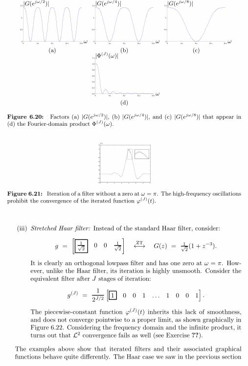
6.2. Scaling Function and Wavelets from Orthogonal Filter Banks 213
0 4Π 8Π 12Π 16Π0
0.5
1.
1.5
ω
|G(ejω/2)|
0 4Π 8Π 12Π 16Π0
0.5
1.
1.5
ω
|G(ejω/4)|
0 4Π 8Π 12Π 16Π0
0.5
1.
1.5
ω
|G(ejω/8)|
(a) (b) (c)
0 4Π 8Π 12Π 16Π0.0
0.2
0.4
0.6
0.8
1.0
1.2
ω
|Φ(J)(ω)|
(d)
Figure 6.20: Factors (a) |G(ejω/2)|, (b) |G(ejω/4)|, and (c) |G(ejω/8)| that appear in(d) the Fourier-domain product Φ(J)(ω).
0 1 2 3 4 5 6 7−0.4
−0.2
0
0.2
0.4
0.6
0.8
1
1.2
1.4φ(J)(t)
Figure 6.21: Iteration of a filter without a zero at ω = π. The high-frequency oscillationsprohibit the convergence of the iterated function ϕ(J)(t).
(iii) Stretched Haar filter: Instead of the standard Haar filter, consider:
g =
[1√2
0 0 1√2
]ZT←→ G(z) = 1√
2(1 + z−3).
It is clearly an orthogonal lowpass filter and has one zero at ω = π. How-ever, unlike the Haar filter, its iteration is highly unsmooth. Consider theequivalent filter after J stages of iteration:
g(J) =1
2J/2
[1 0 0 1 . . . 1 0 0 1
].
The piecewise-constant function ϕ(J)(t) inherits this lack of smoothness,and does not converge pointwise to a proper limit, as shown graphically inFigure 6.22. Considering the frequency domain and the infinite product, itturns out that L2 convergence fails as well (see Exercise ??).
The examples above show that iterated filters and their associated graphicalfunctions behave quite differently. The Haar case we saw in the previous section
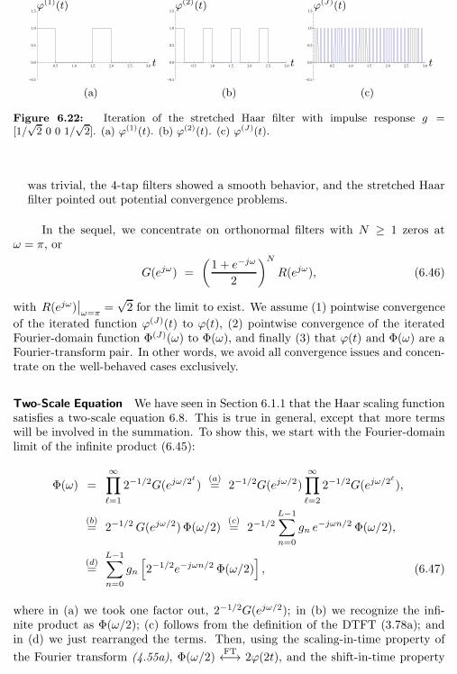
214 Chapter 6. Wavelet Bases, Frames and Transforms on Functions
0.5 1.0 1.5 2.0 2.5 3.0
-0.5
0.0
0.5
1.0
1.5
t
ϕ(1)(t)
0.5 1.0 1.5 2.0 2.5 3.0
-0.5
0.0
0.5
1.0
1.5
t
ϕ(2)(t)
0.5 1.0 1.5 2.0 2.5 3.0
-0.5
0.0
0.5
1.0
1.5
t
ϕ(J)(t)
(a) (b) (c)
Figure 6.22: Iteration of the stretched Haar filter with impulse response g =[1/√2 0 0 1/
√2]. (a) ϕ(1)(t). (b) ϕ(2)(t). (c) ϕ(J)(t).
was trivial, the 4-tap filters showed a smooth behavior, and the stretched Haarfilter pointed out potential convergence problems.
In the sequel, we concentrate on orthonormal filters with N ≥ 1 zeros atω = π, or
G(ejω) =
(1 + e−jω
2
)NR(ejω), (6.46)
with R(ejω)∣∣ω=π
=√2 for the limit to exist. We assume (1) pointwise convergence
of the iterated function ϕ(J)(t) to ϕ(t), (2) pointwise convergence of the iteratedFourier-domain function Φ(J)(ω) to Φ(ω), and finally (3) that ϕ(t) and Φ(ω) are aFourier-transform pair. In other words, we avoid all convergence issues and concen-trate on the well-behaved cases exclusively.
Two-Scale Equation We have seen in Section 6.1.1 that the Haar scaling functionsatisfies a two-scale equation 6.8. This is true in general, except that more termswill be involved in the summation. To show this, we start with the Fourier-domainlimit of the infinite product (6.45):
Φ(ω) =
∞∏
ℓ=1
2−1/2G(ejω/2ℓ
)(a)= 2−1/2G(ejω/2)
∞∏
ℓ=2
2−1/2G(ejω/2ℓ
),
(b)= 2−1/2G(ejω/2)Φ(ω/2)
(c)= 2−1/2
L−1∑
n=0
gn e−jωn/2 Φ(ω/2),
(d)=
L−1∑
n=0
gn
[2−1/2e−jωn/2 Φ(ω/2)
], (6.47)
where in (a) we took one factor out, 2−1/2G(ejω/2); in (b) we recognize the infi-nite product as Φ(ω/2); (c) follows from the definition of the DTFT (3.78a); andin (d) we just rearranged the terms. Then, using the scaling-in-time property of
the Fourier transform (4.55a), Φ(ω/2)FT←→ 2ϕ(2t), and the shift-in-time property
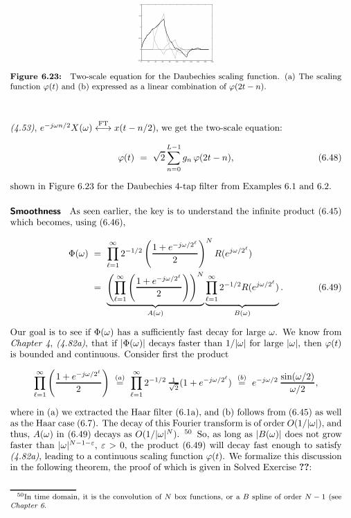
6.2. Scaling Function and Wavelets from Orthogonal Filter Banks 215
0 20 40 60 80 100 120 140 160 180 200−0.5
0
0.5
1
1.5
2
Figure 6.23: Two-scale equation for the Daubechies scaling function. (a) The scalingfunction ϕ(t) and (b) expressed as a linear combination of ϕ(2t − n).
(4.53), e−jωn/2X(ω)FT←→ x(t− n/2), we get the two-scale equation:
ϕ(t) =√2L−1∑
n=0
gn ϕ(2t− n), (6.48)
shown in Figure 6.23 for the Daubechies 4-tap filter from Examples 6.1 and 6.2.
Smoothness As seen earlier, the key is to understand the infinite product (6.45)which becomes, using (6.46),
Φ(ω) =
∞∏
ℓ=1
2−1/2
(1 + e−jω/2
ℓ
2
)N
R(ejω/2ℓ
)
=
( ∞∏
ℓ=1
(1 + e−jω/2
ℓ
2
))N
︸ ︷︷ ︸A(ω)
∞∏
ℓ=1
2−1/2R(ejω/2ℓ
)
︸ ︷︷ ︸B(ω)
. (6.49)
Our goal is to see if Φ(ω) has a sufficiently fast decay for large ω. We know fromChapter 4, (4.82a), that if |Φ(ω)| decays faster than 1/|ω| for large |ω|, then ϕ(t)is bounded and continuous. Consider first the product
∞∏
ℓ=1
(1 + e−jω/2
ℓ
2
)(a)=
∞∏
ℓ=1
2−1/2 1√2(1 + e−jω/2
ℓ
)(b)= e−jω/2
sin(ω/2)
ω/2,
where in (a) we extracted the Haar filter (6.1a), and (b) follows from (6.45) as wellas the Haar case (6.7). The decay of this Fourier transform is of order O(1/|ω|), andthus, A(ω) in (6.49) decays as O(1/|ω|N ). 50 So, as long as |B(ω)| does not growfaster than |ω|N−1−ε, ε > 0, the product (6.49) will decay fast enough to satisfy(4.82a), leading to a continuous scaling function ϕ(t). We formalize this discussionin the following theorem, the proof of which is given in Solved Exercise ??:
50In time domain, it is the convolution of N box functions, or a B spline of order N − 1 (seeChapter 6.
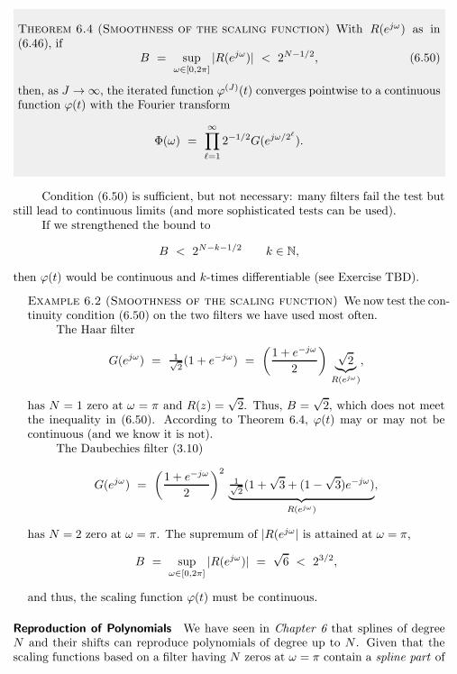
216 Chapter 6. Wavelet Bases, Frames and Transforms on Functions
Theorem 6.4 (Smoothness of the scaling function) With R(ejω) as in(6.46), if
B = supω∈[0,2π]
|R(ejω)| < 2N−1/2, (6.50)
then, as J →∞, the iterated function ϕ(J)(t) converges pointwise to a continuousfunction ϕ(t) with the Fourier transform
Φ(ω) =
∞∏
ℓ=1
2−1/2G(ejω/2ℓ
).
Condition (6.50) is sufficient, but not necessary: many filters fail the test butstill lead to continuous limits (and more sophisticated tests can be used).
If we strengthened the bound to
B < 2N−k−1/2 k ∈ N,
then ϕ(t) would be continuous and k-times differentiable (see Exercise TBD).
Example 6.2 (Smoothness of the scaling function) We now test the con-tinuity condition (6.50) on the two filters we have used most often.
The Haar filter
G(ejω) = 1√2(1 + e−jω) =
(1 + e−jω
2
) √2︸︷︷︸
R(ejω)
,
has N = 1 zero at ω = π and R(z) =√2. Thus, B =
√2, which does not meet
the inequality in (6.50). According to Theorem 6.4, ϕ(t) may or may not becontinuous (and we know it is not).
The Daubechies filter (3.10)
G(ejω) =
(1 + e−jω
2
)21√2(1 +
√3 + (1 −
√3)e−jω)
︸ ︷︷ ︸R(ejω)
,
has N = 2 zero at ω = π. The supremum of |R(ejω | is attained at ω = π,
B = supω∈[0,2π]
|R(ejω)| =√6 < 23/2,
and thus, the scaling function ϕ(t) must be continuous.
Reproduction of Polynomials We have seen in Chapter 6 that splines of degreeN and their shifts can reproduce polynomials of degree up to N . Given that thescaling functions based on a filter having N zeros at ω = π contain a spline part of
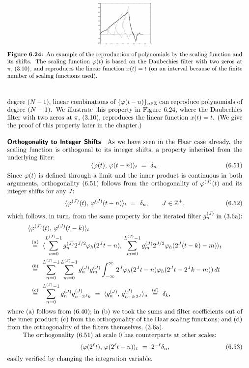
6.2. Scaling Function and Wavelets from Orthogonal Filter Banks 217
0 50 100 150 200 250 300 350 400 450−100
−50
0
50
100
150
200
250
300
350
Figure 6.24: An example of the reproduction of polynomials by the scaling function andits shifts. The scaling function ϕ(t) is based on the Daubechies filter with two zeros atπ, (3.10), and reproduces the linear function x(t) = t (on an interval because of the finitenumber of scaling functions used).
degree (N − 1), linear combinations of ϕ(t− n)n∈Z can reproduce polynomials ofdegree (N − 1). We illustrate this property in Figure 6.24, where the Daubechiesfilter with two zeros at π, (3.10), reproduces the linear function x(t) = t. (We givethe proof of this property later in the chapter.)
Orthogonality to Integer Shifts As we have seen in the Haar case already, thescaling function is orthogonal to its integer shifts, a property inherited from theunderlying filter:
〈ϕ(t), ϕ(t− n)〉t = δn. (6.51)
Since ϕ(t) is defined through a limit and the inner product is continuous in botharguments, orthogonality (6.51) follows from the orthogonality of ϕ(J)(t) and itsinteger shifts for any J :
〈ϕ(J)(t), ϕ(J)(t− n)〉t = δn, J ∈ Z+, (6.52)
which follows, in turn, from the same property for the iterated filter g(J)n in (3.6a):
〈ϕ(J)(t), ϕ(J)(t− k)〉t
(a)= 〈
L(J)−1∑
n=0
g(J)n
2J/2ϕh(2J t− n),
L(J)−1∑
m=0
g(J)m
2J/2ϕh(2J(t− k)−m)〉t
(b)=
L(J)−1∑
n=0
L(J)−1∑
m=0
g(J)ng(J)m
∫ ∞
−∞2Jϕh(2
J t− n)ϕh(2J t− 2Jk −m)) dt
(c)=
L(J)−1∑
n=0
g(J)ng(J)
n−2Jk = 〈g(J)n, g
(J)
n−k 2J 〉n(d)= δk,
where (a) follows from (6.40); in (b) we took the sums and filter coefficients out ofthe inner product; (c) from the orthogonality of the Haar scaling functions; and (d)from the orthogonality of the filters themselves, (3.6a).
The orthogonality (6.51) at scale 0 has counterparts at other scales:
〈ϕ(2ℓt), ϕ(2ℓt− n)〉t = 2−ℓδn, (6.53)
easily verified by changing the integration variable.
218 Chapter 6. Wavelet Bases, Frames and Transforms on Functions
6.2.3 Wavelet Function and its Properties
The scaling function we have just seen is lowpass in nature (if the underlying filterg is lowpass in nature). Similarly to what we have done for the scaling function,we can construct a wavelet function (or, simply wavelet) that will be bandpass innature (if the underlying filter h is highpass in nature).
We thus associate a piecewise-constant function ψ(J)(t) to h(J)n , the impulse
response of (6.37b), in such a way that ψ(J)(t) is of finite length and of norm 1;we use the same arguments as before to determine the width and height of thepiecewise segments, leading to
ψ(J)(t) = 2J/2 h(J)n
n
2J≤ t <
n+ 1
2J. (6.54)
Unlike ϕ(J)(t), our new object of interest ψ(J)(t) is a bandpass function. In partic-ular, because H(ejω)
∣∣ω=π
= 0, its Fourier transform Ψ(ω) satisfies
Ψ(ω)|ω=0 = 0.
Again, we are interested in what happens when J →∞. Clearly, this involvesan infinite product, but it is the same infinite product we studied for the convergenceof ϕ(J)(t) towards ϕ(t). In short, we assume this question to be settled. Thedevelopment parallels the one for the scaling function, with the important twist of
consistently replacing the lowpass filter G(z2J−1
) by the highpass filter H(z2J−1
).We do not repeat the details, but rather indicate the main points. Equation (6.44)becomes
Ψ(J)(ω) = Φ(J)h
(ω)H(ejω/2)
J∏
ℓ=2
G(ejω/2ℓ
). (6.55)
Similarly to the scaling function, we define the wavelet as the limit of ψ(J)(t)or Ψ(J)(ω), where we now assume that both are well defined and form a Fourier-transform pair.
Definition 6.5 (Wavelet) Assuming the limit to exist, we define the waveletin time and frequency domains to be
ψ(t) = limJ→∞
ψ(J)(t), (6.56a)
Ψ(ω) = limJ→∞
Ψ(J)(ω). (6.56b)
From (6.55) and using the steps leading to (6.45), we can write
Ψ(ω) = 2−1/2H(ejω/2)
∞∏
ℓ=2
2−1/2G(ejω/2ℓ
). (6.57)
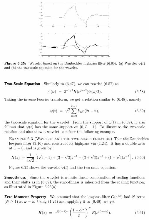
6.2. Scaling Function and Wavelets from Orthogonal Filter Banks 219
0 0.5 1 1.5 2 2.5 3−1.5
−1
−0.5
0
0.5
1
1.5
2
0 20 40 60 80 100 120 140 160 180 200−1.5
−1
−0.5
0
0.5
1
1.5
2
Figure 6.25: Wavelet based on the Daubechies highpass filter (6.60). (a) Wavelet ψ(t)and (b) the two-scale equation for the wavelet.
Two-Scale Equation Similarly to (6.47), we can rewrite (6.57) as
Ψ(ω) = 2−1/2H(ejω/2)Φ(ω/2). (6.58)
Taking the inverse Fourier transform, we get a relation similar to (6.48), namely
ψ(t) =√2L−1∑
n=0
hnϕ(2t− n), (6.59)
the two-scale equation for the wavelet. From the support of ϕ(t) in (6.39), it alsofollows that ψ(t) has the same support on [0, L − 1]. To illustrate the two-scalerelation and also show a wavelet, consider the following example.
Example 6.3 (Wavelet and the two-scale equation) Take the Daubechieslowpass filter (3.10) and construct its highpass via (1.24). It has a double zeroat ω = 0, and is given by:
H(z) =1
4√2
[(√3− 1) + (3−
√3)z−1 − (3 +
√3)z−2 + (1 +
√3)z−3
]. (6.60)
Figure 6.25 shows the wavelet ψ(t) and the two-scale equation.
Smoothness Since the wavelet is a finite linear combination of scaling functionsand their shifts as in (6.59), the smoothness is inherited from the scaling function,as illustrated in Figure 6.25(a).
Zero-Moment Property We assumed that the lowpass filter G(ejω) had N zeros(N ≥ 1) at ω = π. Using (1.24) and applying it to (6.46), we get
H(z) = ej(L−1)ω
(1− ejω
2
)NR(ej(ω+π)). (6.61)
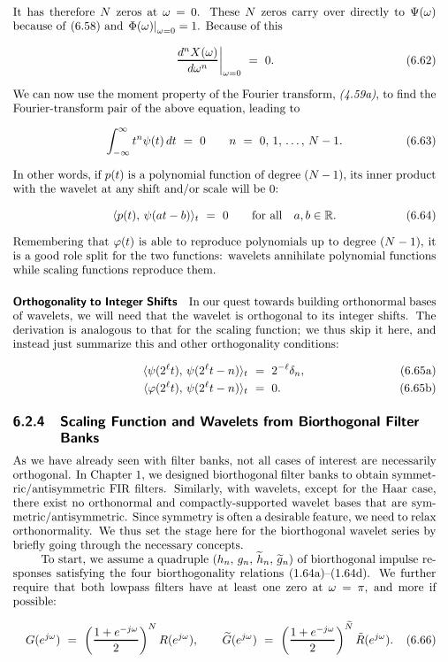
220 Chapter 6. Wavelet Bases, Frames and Transforms on Functions
It has therefore N zeros at ω = 0. These N zeros carry over directly to Ψ(ω)because of (6.58) and Φ(ω)|
ω=0 = 1. Because of this
dnX(ω)
dωn
∣∣∣∣ω=0
= 0. (6.62)
We can now use the moment property of the Fourier transform, (4.59a), to find theFourier-transform pair of the above equation, leading to
∫ ∞
−∞tnψ(t) dt = 0 n = 0, 1, . . . , N − 1. (6.63)
In other words, if p(t) is a polynomial function of degree (N − 1), its inner productwith the wavelet at any shift and/or scale will be 0:
〈p(t), ψ(at− b)〉t = 0 for all a, b ∈ R. (6.64)
Remembering that ϕ(t) is able to reproduce polynomials up to degree (N − 1), itis a good role split for the two functions: wavelets annihilate polynomial functionswhile scaling functions reproduce them.
Orthogonality to Integer Shifts In our quest towards building orthonormal basesof wavelets, we will need that the wavelet is orthogonal to its integer shifts. Thederivation is analogous to that for the scaling function; we thus skip it here, andinstead just summarize this and other orthogonality conditions:
〈ψ(2ℓt), ψ(2ℓt− n)〉t = 2−ℓδn, (6.65a)
〈ϕ(2ℓt), ψ(2ℓt− n)〉t = 0. (6.65b)
6.2.4 Scaling Function and Wavelets from Biorthogonal Filter
Banks
As we have already seen with filter banks, not all cases of interest are necessarilyorthogonal. In Chapter 1, we designed biorthogonal filter banks to obtain symmet-ric/antisymmetric FIR filters. Similarly, with wavelets, except for the Haar case,there exist no orthonormal and compactly-supported wavelet bases that are sym-metric/antisymmetric. Since symmetry is often a desirable feature, we need to relaxorthonormality. We thus set the stage here for the biorthogonal wavelet series bybriefly going through the necessary concepts.
To start, we assume a quadruple (hn, gn, hn, gn) of biorthogonal impulse re-sponses satisfying the four biorthogonality relations (1.64a)–(1.64d). We furtherrequire that both lowpass filters have at least one zero at ω = π, and more ifpossible:
G(ejω) =
(1 + e−jω
2
)NR(ejω), G(ejω) =
(1 + e−jω
2
)N
R(ejω). (6.66)
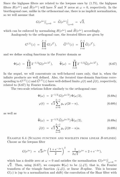
6.2. Scaling Function and Wavelets from Orthogonal Filter Banks 221
Since the highpass filters are related to the lowpass ones by (1.75), the highpass
filters H(ejω) and H(ejω) will have N and N zeros at ω = 0, respectively. In thebiorthogonal case, unlike in the orthonormal one, there is no implicit normalization,so we will assume that
G(ejω)∣∣ω=0
= G(ejω)∣∣∣ω=0
=√2,
which can be enforced by normalizing H(ejω) and H(ejω) accordingly.Analogously to the orthogonal case, the iterated filters are given by
G(J)(z) =
J−1∏
ℓ=0
G(z2ℓ
), G(J)(z) =
J−1∏
ℓ=0
G(z2ℓ
),
and we define scaling functions in the Fourier domain as
Φ(ω) =
∞∏
ℓ=0
2−1/2G(ejω/2ℓ
), Φ(ω) =
∞∏
ℓ=0
2−1/2G(ejω/2ℓ
). (6.67)
In the sequel, we will concentrate on well-behaved cases only, that is, when theinfinite products are well defined. Also, the iterated time-domain functions corre-sponding to G(J)(z) and G(J)(z) have well-defined limits ϕ(t) and ϕ(t), respectively,related to (6.67) by Fourier transform.
The two-scale relations follow similarly to the orthogonal case:
Φ(ω) = 2−1/2G(ejω/2)Φ(ω/2), (6.68a)
ϕ(t) =√2
L−1∑
n=0
gn ϕ(2t− n), (6.68b)
as well as
Φ(ω) = 2−1/2 G(ejω/2) Φ(ω/2), (6.69a)
ϕ(t) =√2
L−1∑
n=0
gn ϕ(2t− n)a. (6.69b)
Example 6.4 (Scaling function and wavelets from linear B-splines)Choose as the lowpass filter
G(ejω) =√2ejω
(1 + e−jω
2
)2
=1
2√2(ejω + 2 + e−jω),
which has a double zero at ω = 0 and satisfies the normalization G(ejω)∣∣ω=0
=√2. Then, using (6.67), we compute Φ(ω) to be (4.47), that is, the Fourier
transform of the triangle function (4.45), or linear B-spline. This is becauseG(z) is (up to a normalization and shift) the convolution of the Haar filter with
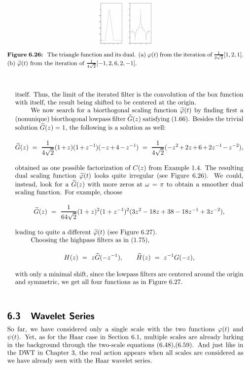
222 Chapter 6. Wavelet Bases, Frames and Transforms on Functions
−1 0 1 2 3
0
0.2
0.4
0.6
0.8
1
0 1 2 3−2
−1
0
1
2
3
4
5
Figure 6.26: The triangle function and its dual. (a) ϕ(t) from the iteration of 1
2√
2[1, 2, 1].
(b) ϕ(t) from the iteration of 1
4√
2[−1, 2, 6, 2,−1].
itself. Thus, the limit of the iterated filter is the convolution of the box functionwith itself, the result being shifted to be centered at the origin.
We now search for a biorthogonal scaling function ϕ(t) by finding first a
(nonunique) biorthogonal lowpass filter G(z) satisfying (1.66). Besides the trivial
solution G(z) = 1, the following is a solution as well:
G(z) =1
4√2(1+z)(1+z−1)(−z+4−z−1) =
1
4√2(−z2+2z+6+2z−1−z−2),
obtained as one possible factorization of C(z) from Example 1.4. The resultingdual scaling function ϕ(t) looks quite irregular (see Figure 6.26). We could,
instead, look for a G(z) with more zeros at ω = π to obtain a smoother dualscaling function. For example, choose
G(z) =1
64√2(1 + z)2(1 + z−1)2(3z2 − 18z + 38− 18z−1 + 3z−2),
leading to quite a different ϕ(t) (see Figure 6.27).Choosing the highpass filters as in (1.75),
H(z) = zG(−z−1), H(z) = z−1G(−z),
with only a minimal shift, since the lowpass filters are centered around the originand symmetric, we get all four functions as in Figure 6.27.
6.3 Wavelet Series
So far, we have considered only a single scale with the two functions ϕ(t) andψ(t). Yet, as for the Haar case in Section 6.1, multiple scales are already lurkingin the background through the two-scale equations (6.48),(6.59). And just like inthe DWT in Chapter 3, the real action appears when all scales are considered aswe have already seen with the Haar wavelet series.
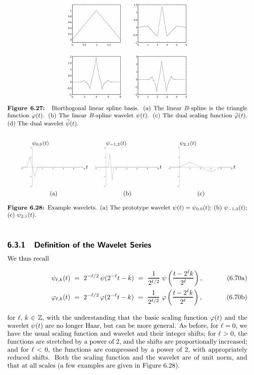
6.3. Wavelet Series 223
0 0.5 1 1.5
0
0.2
0.4
0.6
0.8
1
0 1 2 3 4 5−1
−0.5
0
0.5
1
1.5
0 2 4 6 8−1
−0.5
0
0.5
1
1.5
2
0 1 2 3 4 5−2
−1
0
1
2
3
Figure 6.27: Biorthogonal linear spline basis. (a) The linear B-spline is the trianglefunction ϕ(t). (b) The linear B-spline wavelet ψ(t). (c) The dual scaling function ϕ(t).
(d) The dual wavelet ψ(t).
-2 2 4 6 8 10
-2
-1
1
2
t
ψ0,0(t)
-2 2 4 6 8 10
-2
-1
1
2
t
ψ−1,2(t)
-2 2 4 6 8 10
-2
-1
1
2
t
ψ2,1(t)
(a) (b) (c)
Figure 6.28: Example wavelets. (a) The prototype wavelet ψ(t) = ψ0,0(t); (b) ψ−1,2(t);(c) ψ2,1(t).
6.3.1 Definition of the Wavelet Series
We thus recall
ψℓ,k(t) = 2−ℓ/2 ψ(2−ℓt− k) =1
2ℓ/2ψ
(t− 2ℓk
2ℓ
), (6.70a)
ϕℓ,k(t) = 2−ℓ/2 ϕ(2−ℓt− k) =1
2ℓ/2ϕ
(t− 2ℓk
2ℓ
), (6.70b)
for ℓ, k ∈ Z, with the understanding that the basic scaling function ϕ(t) and thewavelet ψ(t) are no longer Haar, but can be more general. As before, for ℓ = 0, wehave the usual scaling function and wavelet and their integer shifts; for ℓ > 0, thefunctions are stretched by a power of 2, and the shifts are proportionally increased;and for ℓ < 0, the functions are compressed by a power of 2, with appropriatelyreduced shifts. Both the scaling function and the wavelet are of unit norm, andthat at all scales (a few examples are given in Figure 6.28).
224 Chapter 6. Wavelet Bases, Frames and Transforms on Functions
Two-Scale Equations at Nonconsecutive Scales Since we want to deal with mul-tiple scales (not just two), we extend the two-scale equations for ϕ(t) and ψ(t) acrossarbitrary scales that are powers of 2:
Φ(ω)(a)= 2−1/2G(ejω/2)Φ(ω/2),
(b)= 2−1G(ejω/2)G(ejω/4)Φ(ω/4),
(c)= 2−1G(2)(ejω/4)Φ(ω/4),
...
= 2−k/2G(k)(ejω/2k
)Φ(ω/2k), (6.71a)
ϕ(t) = 2k/2L−1∑
n=0
g(k)n
ϕ(2kt− n), (6.71b)
for k ∈ Z+, where both (a) and (b) follow from the two-scale equation in the Fourierdomain, (6.47); (c) from the expression for the equivalent filter, (6.37a); and (d) byrepeatedly applying the same (see Exercise ??). The last expression is obtained byapplying the inverse DTFT to (6.71a).
Using an analogous derivation for the wavelet, we get
Ψ(ω) = 2−k/2H(k)(ejω/2k
)Φ(ω/2k), (6.72a)
ψ(t) = 2k/2L−1∑
n=0
h(k)nϕ(2kt− n), (6.72b)
for k = 2, 3, . . .. The attractiveness of the above expressions lies in their abilityto express any ϕℓ,k(t), ψℓ,k(t), in terms of a linear combination of an appropriatelyscaled ϕ(t), where the linear combination is given by the coefficients of an equivalent
filter g(k)n or h
(k)n . We are now ready for the main result of this chapter:
Theorem 6.6 (Orthonormal basis for L2(R)) The continuous-time waveletψ(t) satisfying (6.59) and its shifts and scales,
ψℓ,k(t) = 1√2ℓψ
(t− 2ℓk
2ℓ
), ℓ, k ∈ Z, (6.73)
form an orthonormal basis for the space of square-integrable functions, L2(R).
Proof. To prove the theorem, we must prove that (i) ψℓ,k(t)ℓ, k∈Z is an orthonormalset and (ii) it is complete. The good news is that most of the hard work has alreadybeen done while studying the DWT in Theorem 3.2, Chapter 3.
6.3. Wavelet Series 225
(i) We have already shown that the wavelets and their shifts are orthonormal at asingle scale, (6.65a), and need to show the same across scales:
〈ψℓ,k(t), ψm,n(t)〉t(a)= 2−ℓ〈ψ0,k(τ ), ψ−i,n(τ )〉τ ,(b)= 2−ℓ〈2i/2
∑
n
h(i)n ϕ−i,2ik+n(τ ), ψ−i,n(τ )〉τ ,
(c)= 2−ℓ+i/2
∑
n
h(i)n 〈ϕ−i,2ik+n(τ ), ψ−i,n(τ )〉τ = 0,
where (a) follows from assuming (without loss of generality) ℓ = m+ i, i > 0, andchange of variable t = 2ℓτ ; (b) from two-scale equation for the wavelet (6.72b);and (c) from the linearity of the inner product as well as orthogonality of thewavelet and scaling function (6.65a).
(ii) The proof of completeness is more involved, and thus, we show it only for theHaar case. Further Reading gives pointers to texts with the full proof. Consider aunit-norm function x(t) such that x(t) = 0 for t < 0 with finite length at most 2J
for some J ∈ Z.51 We approximate x(t) by a piecewise-constant approximationat scale ℓ, (where ℓ≪ J), or
x(ℓ)(t) = 2−ℓ∫ 2ℓ(k+1)
2ℓk
x(τ ) dτ, 2ℓk ≤ t < 2ℓ(k + 1),
(a)=
∑
k∈Z
(∫
τ∈R
x(τ )ϕℓ,k(τ ) dτ
)ϕℓ,k(t),
(b)=
∑
k∈Z
〈x, ϕℓ,k〉ϕℓ,k(t)(c)=
∑
k∈Z
α(ℓ)k ϕℓ,k(t), (6.74a)
where (a) follows from (6.16b); (b) from the definition of the inner product; and
in (c) we introduced α(ℓ)k = 〈x, ϕℓ,k〉.
Because of the finite-length assumption of x(t), the sequence α(ℓ)k is also of
finite length (of degree 2J−ℓ). Since x(t) is of norm 1 and the approximation in
(6.74a) is a projection, ‖α(ℓ)k ‖ ≤ 1. Thus, we can apply Theorem 3.2 and represent
the sequence α(ℓ)k by discrete Haar wavelets only
α(ℓ)k =
∑
n∈Z
∑
i∈Z+
β(i)n h
(i)
k−2in.
Since the expression (6.74a) is the piecewise-constant interpolation of the sequence
α(ℓ)k , together with proper scaling and normalization, by linearity, we can apply
this interpolation to the discrete Haar wavelets used to represent α(ℓ)k , which leads
51Both of these restrictions are inconsequential; the former because a general function can bedecomposed into a function nonzero on t > 0 and t ≤ 0, the latter because the fraction of theenergy of x(t) outside of the interval under consideration can be made arbitrarily small by makingJ arbitrarily large.
226 Chapter 6. Wavelet Bases, Frames and Transforms on Functions
to a continuous-time Haar wavelet representation of x(ℓ)(t):
x(ℓ)(t) =∑
k∈Z
α(ℓ)k ϕℓ,k(t),
=∑
k∈Z
∑
n∈Z
∑
i∈Z+
β(i)n h
(i)
k−2inϕℓ,k(t),
=∑
n∈Z
∑
i∈Z+
β(i)n ψℓ+i,n2i(t).
This last statement follows from h(i) being of length 2i. Thus, for a fixed n andi,
∑k∈Z
h(i)
k−2inϕℓ,k(t) will equal the Haar wavelet of length 2i2ℓ = 2i+ℓ at shift
n2i. Again by Theorem 3.2, this representation is exact.What remains to be shown is that x(ℓ)(t) can be made arbitrarily close, in
L2 norm, to x(t). This is achieved by letting ℓ → −∞ and using the fact thatpiecewise-constant functions are dense in L2(R);52 we get
limi→−∞
‖x(t)− x(ℓ)(t)‖ = 0.
TBD: Might be expanded.
The proof once more shows the intimate relation between the DWT from Chapter 3and the wavelet series from this chapter.
Definition We can now formally define the wavelet series:
Definition 6.7 (Wavelet series) The wavelet series of a function x(t) is afunction of ℓ, k ∈ Z given by
β(ℓ)k
= 〈x, ψℓ,k〉 =
∫ ∞
−∞x(t)ψℓ,k(t) dt, ℓ, k ∈ Z, (6.75a)
with ψℓ,k(t) the prototype wavelet. The inverse wavelet series is given by
x(t) =∑
ℓ∈Z
∑
k∈Z
β(ℓ)kψℓ,k(t). (6.75b)
In the above, β(ℓ) are the wavelet coefficients.To denote such a wavelet series pair, we write:
x(t)WS←→ β
(ℓ)k.
We derived such bases already and we will see other constructions when wetalk about multiresolution analysis.
52 That is, any L2 function can be approximated arbitrarily closely by a piecewise-constantfunction over intervals that tend to 0. This is a standard result but technical, and thus we justuse it without proof.
6.3. Wavelet Series 227
6.3.2 Properties of the Wavelet Series
We now consider some of the properties of the wavelet series. Many follow from theproperties of the wavelet (Section 6.2.3) or of the DWT (Chapter 3), and thus ourtreatment will be brief.
Linearity The wavelet series operator is a linear operator, or,
a x(t) + b y(t)WS←→ a β
(ℓ)k
+ b β(ℓ)k. (6.76)
Shift in Time A shift in time by 2mn, m, n ∈ Z, results in
x(t− 2mn)WS←→ β
(ℓ)k−2mn, ℓ ≤ m. (6.77)
This is a restrictive condition as it holds only for scales smaller than m. In otherwords, only a function x(t) that has a scale-limited expansion, that is, it can bewritten as
x(t) =
m∑
ℓ=−∞
∑
k∈Z
β(ℓ)kψℓ,k(t),
will possess the shift-in-time property for all (of its existing) scales. This is acounterpart to the shift-in-time property of the DWT, (3.17), and the fact that theDWT is periodically shift varying.
Scaling in Time Scaling in time by 2−m, m ∈ Z, results in
x(2−mt)WS←→ 2m/2β
(ℓ−m)k
. (6.78)
Parseval’s Equality The wavelet series operator is a unitary operator and thuspreserves the Euclidean norm (see (2.53)):
‖x‖2 =
∫ ∞
−∞|x(t)|2 dt =
∑
ℓ∈Z
∑
k∈Z
|β(ℓ)k|2. (6.79)
Time-Frequency Localization Assume that the wavelet ψ(t) is centered aroundt = 0 in time and ω = 3π/4 in frequency (that is, it is a bandpass filter with thesupport of approximately [π/2, π]). Then, from (6.70a), ψℓ,0(t) is centered aroundω = 2−ℓ(3π/4) in frequency (see Figure 6.29).
With our assumption of g being a causal FIR filter of length L, the support intime of the wavelets is easy to characterize. Since the support of ψ(t) is [0, L− 1],
support(ψℓ,k(t)) ⊆ [2ℓk, 2ℓ(k + L− 1)). (6.80)
Because of the FIR assumption, the frequency localization is less precise (no com-pact support in frequency), but the center frequency is around 2−ℓ(3π/4) and thepassband is mostly in an octave band,
support(Ψℓ,k(ω)) ∼ [2−ℓπ
2, 2−ℓπ]. (6.81)
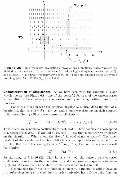
228 Chapter 6. Wavelet Bases, Frames and Transforms on Functions
Figure 6.29: Time-frequency localization of wavelet basis functions. Three wavelets arehighlighted: at scale ℓ = 0, ψ(t); at scale ℓ = −1, a higher-frequency wavelet ψ−1,7(t);and at scale ℓ = 2, a lower-frequency wavelet ψ2,1(t). These are centered along the dyadicsampling grid [2ℓk 2−ℓ(3π/4)], for ℓ, k ∈ Z.
Characterization of Singularities As we have seen with the example of Haarwavelet series (see Figure 6.8), one of the powerful features of the wavelet seriesis its ability to characterize both the position and type of singularities present in afunction.
Consider a function with the simplest singularity, a Dirac delta function at alocation t0, that is, x(t) = δ(t− t0). At scale ℓ, only wavelets having their support(6.80) straddling t0 will produce nonzero coefficients,
β(ℓ)k6= 0 for ⌊t0/2ℓ⌋ − L < k ≤ ⌊t0/2ℓ⌋. (6.82)
Thus, there are L nonzero coefficients at each scale. These coefficients correspondto a region of size 2ℓ(L−1) around t0, or, as ℓ→ −∞, they focus arbitrarily closelyon the singularity. What about the size of the coefficients at scale ℓ? The innerproduct of the wavelet with a Dirac delta function simply picks out a value of thewavelet. Because of the scaling factor 2−ℓ/2 in (6.70a), the nonzero coefficients willbe of order
|β(ℓ)k| ∼ O(2−ℓ/2) (6.83)
for the range of k in (6.82). That is, as ℓ → −∞, the nonzero wavelet seriescoefficients zoom in onto the discontinuity, and they grow at a specific rate givenby (6.83). An example for the Haar wavelet was shown in Figure 6.8.
Generalizing the Dirac delta function singularity, a function is said to have annth-order singularity at t0 when its nth-order derivative has a Dirac delta function
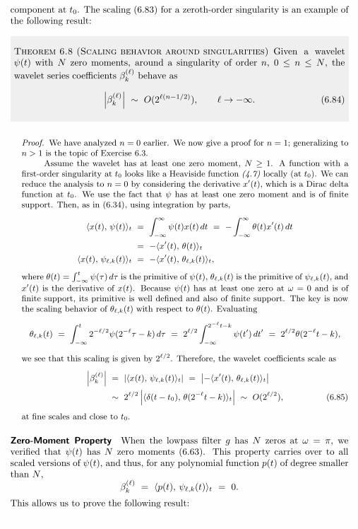
6.3. Wavelet Series 229
component at t0. The scaling (6.83) for a zeroth-order singularity is an example ofthe following result:
Theorem 6.8 (Scaling behavior around singularities) Given a waveletψ(t) with N zero moments, around a singularity of order n, 0 ≤ n ≤ N , the
wavelet series coefficients β(ℓ)k
behave as
∣∣∣β(ℓ)k
∣∣∣ ∼ O(2ℓ(n−1/2)), ℓ→ −∞. (6.84)
Proof. We have analyzed n = 0 earlier. We now give a proof for n = 1; generalizing ton > 1 is the topic of Exercise 6.3.
Assume the wavelet has at least one zero moment, N ≥ 1. A function with afirst-order singularity at t0 looks like a Heaviside function (4.7) locally (at t0). We canreduce the analysis to n = 0 by considering the derivative x′(t), which is a Dirac deltafunction at t0. We use the fact that ψ has at least one zero moment and is of finitesupport. Then, as in (6.34), using integration by parts,
〈x(t), ψ(t)〉t =
∫ ∞
−∞ψ(t)x(t)dt = −
∫ ∞
−∞θ(t)x′(t) dt
= −〈x′(t), θ(t)〉t〈x(t), ψℓ,k(t)〉t = −〈x′(t), θℓ,k(t)〉t,
where θ(t) =∫ t−∞ ψ(τ ) dτ is the primitive of ψ(t), θℓ,k(t) is the primitive of ψℓ,k(t), and
x′(t) is the derivative of x(t). Because ψ(t) has at least one zero at ω = 0 and is offinite support, its primitive is well defined and also of finite support. The key is nowthe scaling behavior of θℓ,k(t) with respect to θ(t). Evaluating
θℓ,k(t) =
∫ t
−∞2−ℓ/2ψ(2−ℓτ − k) dτ = 2ℓ/2
∫ 2−ℓt−k
−∞ψ(t′) dt′ = 2ℓ/2θ(2−ℓt− k),
we see that this scaling is given by 2ℓ/2. Therefore, the wavelet coefficients scale as∣∣∣β(ℓ)k
∣∣∣ = |〈x(t), ψℓ,k(t)〉t| =∣∣−〈x′(t), θℓ,k(t)〉t
∣∣
∼ 2ℓ/2∣∣∣〈δ(t− t0), θ(2−ℓt− k)〉t
∣∣∣ ∼ O(2ℓ/2), (6.85)
at fine scales and close to t0.
Zero-Moment Property When the lowpass filter g has N zeros at ω = π, weverified that ψ(t) has N zero moments (6.63). This property carries over to allscaled versions of ψ(t), and thus, for any polynomial function p(t) of degree smallerthan N ,
β(ℓ)k
= 〈p(t), ψℓ,k(t)〉t = 0.
This allows us to prove the following result:
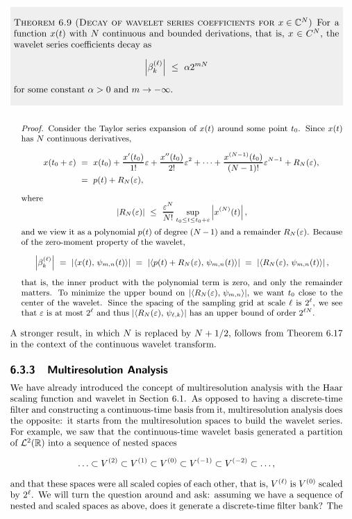
230 Chapter 6. Wavelet Bases, Frames and Transforms on Functions
Theorem 6.9 (Decay of wavelet series coefficients for x ∈ CN) For afunction x(t) with N continuous and bounded derivations, that is, x ∈ CN , thewavelet series coefficients decay as
∣∣∣β(ℓ)k
∣∣∣ ≤ α2mN
for some constant α > 0 and m→ −∞.
Proof. Consider the Taylor series expansion of x(t) around some point t0. Since x(t)has N continuous derivatives,
x(t0 + ε) = x(t0) +x′(t0)
1!ε+
x′′(t0)
2!ε2 + · · ·+ x(N−1)(t0)
(N − 1)!εN−1 +RN (ε),
= p(t) +RN(ε),
where
|RN (ε)| ≤ εN
N !sup
t0≤t≤t0+ε
∣∣∣x(N)(t)∣∣∣ ,
and we view it as a polynomial p(t) of degree (N − 1) and a remainder RN (ε). Becauseof the zero-moment property of the wavelet,
∣∣∣β(ℓ)k
∣∣∣ = |〈x(t), ψm,n(t)〉| = |〈p(t) +RN (ε), ψm,n(t)〉| = |〈RN (ε), ψm,n(t)〉| ,
that is, the inner product with the polynomial term is zero, and only the remaindermatters. To minimize the upper bound on |〈RN (ε), ψm,n〉|, we want t0 close to thecenter of the wavelet. Since the spacing of the sampling grid at scale ℓ is 2ℓ, we seethat ε is at most 2ℓ and thus |〈RN (ε), ψℓ,k〉| has an upper bound of order 2ℓN .
A stronger result, in which N is replaced by N + 1/2, follows from Theorem 6.17in the context of the continuous wavelet transform.
6.3.3 Multiresolution Analysis
We have already introduced the concept of multiresolution analysis with the Haarscaling function and wavelet in Section 6.1. As opposed to having a discrete-timefilter and constructing a continuous-time basis from it, multiresolution analysis doesthe opposite: it starts from the multiresolution spaces to build the wavelet series.For example, we saw that the continuous-time wavelet basis generated a partitionof L2(R) into a sequence of nested spaces
. . . ⊂ V (2) ⊂ V (1) ⊂ V (0) ⊂ V (−1) ⊂ V (−2) ⊂ . . . ,
and that these spaces were all scaled copies of each other, that is, V (ℓ) is V (0) scaledby 2ℓ. We will turn the question around and ask: assuming we have a sequence ofnested and scaled spaces as above, does it generate a discrete-time filter bank? The
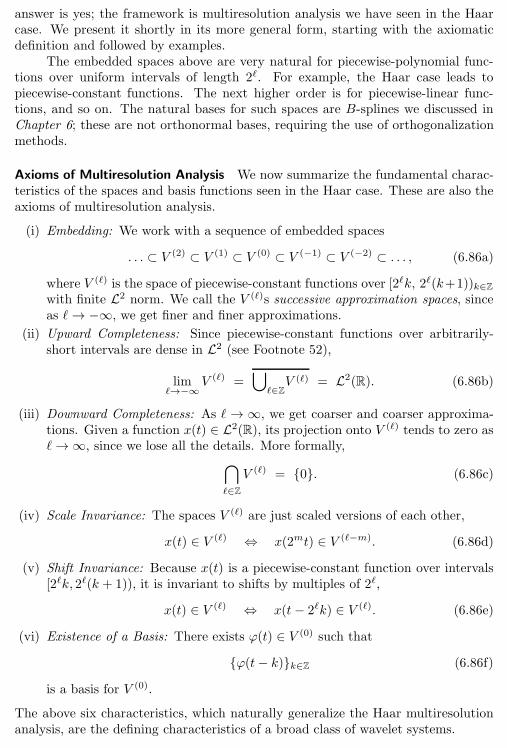
6.3. Wavelet Series 231
answer is yes; the framework is multiresolution analysis we have seen in the Haarcase. We present it shortly in its more general form, starting with the axiomaticdefinition and followed by examples.
The embedded spaces above are very natural for piecewise-polynomial func-tions over uniform intervals of length 2ℓ. For example, the Haar case leads topiecewise-constant functions. The next higher order is for piecewise-linear func-tions, and so on. The natural bases for such spaces are B-splines we discussed inChapter 6; these are not orthonormal bases, requiring the use of orthogonalizationmethods.
Axioms of Multiresolution Analysis We now summarize the fundamental charac-teristics of the spaces and basis functions seen in the Haar case. These are also theaxioms of multiresolution analysis.
(i) Embedding: We work with a sequence of embedded spaces
. . . ⊂ V (2) ⊂ V (1) ⊂ V (0) ⊂ V (−1) ⊂ V (−2) ⊂ . . . , (6.86a)
where V (ℓ) is the space of piecewise-constant functions over [2ℓk, 2ℓ(k+1))k∈Z
with finite L2 norm. We call the V (ℓ)s successive approximation spaces, sinceas ℓ→ −∞, we get finer and finer approximations.
(ii) Upward Completeness: Since piecewise-constant functions over arbitrarily-short intervals are dense in L2 (see Footnote 52),
limℓ→−∞
V (ℓ) =⋃
ℓ∈Z
V (ℓ) = L2(R). (6.86b)
(iii) Downward Completeness: As ℓ → ∞, we get coarser and coarser approxima-tions. Given a function x(t) ∈ L2(R), its projection onto V (ℓ) tends to zero asℓ→∞, since we lose all the details. More formally,
⋂
ℓ∈Z
V (ℓ) = 0. (6.86c)
(iv) Scale Invariance: The spaces V (ℓ) are just scaled versions of each other,
x(t) ∈ V (ℓ) ⇔ x(2mt) ∈ V (ℓ−m). (6.86d)
(v) Shift Invariance: Because x(t) is a piecewise-constant function over intervals[2ℓk, 2ℓ(k + 1)), it is invariant to shifts by multiples of 2ℓ,
x(t) ∈ V (ℓ) ⇔ x(t− 2ℓk) ∈ V (ℓ). (6.86e)
(vi) Existence of a Basis: There exists ϕ(t) ∈ V (0) such that
ϕ(t− k)k∈Z (6.86f)
is a basis for V (0).
The above six characteristics, which naturally generalize the Haar multiresolutionanalysis, are the defining characteristics of a broad class of wavelet systems.
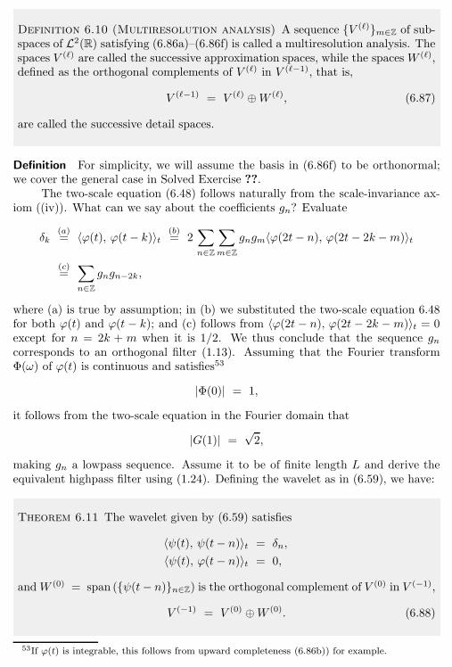
232 Chapter 6. Wavelet Bases, Frames and Transforms on Functions
Definition 6.10 (Multiresolution analysis) A sequence V (ℓ)m∈Z of sub-spaces of L2(R) satisfying (6.86a)–(6.86f) is called a multiresolution analysis. Thespaces V (ℓ) are called the successive approximation spaces, while the spacesW (ℓ),defined as the orthogonal complements of V (ℓ) in V (ℓ−1), that is,
V (ℓ−1) = V (ℓ) ⊕W (ℓ), (6.87)
are called the successive detail spaces.
Definition For simplicity, we will assume the basis in (6.86f) to be orthonormal;we cover the general case in Solved Exercise ??.
The two-scale equation (6.48) follows naturally from the scale-invariance ax-iom ((iv)). What can we say about the coefficients gn? Evaluate
δk(a)= 〈ϕ(t), ϕ(t− k)〉t
(b)= 2
∑
n∈Z
∑
m∈Z
gngm〈ϕ(2t− n), ϕ(2t− 2k −m)〉t
(c)=∑
n∈Z
gngn−2k,
where (a) is true by assumption; in (b) we substituted the two-scale equation 6.48for both ϕ(t) and ϕ(t − k); and (c) follows from 〈ϕ(2t − n), ϕ(2t − 2k −m)〉t = 0except for n = 2k + m when it is 1/2. We thus conclude that the sequence gncorresponds to an orthogonal filter (1.13). Assuming that the Fourier transformΦ(ω) of ϕ(t) is continuous and satisfies53
|Φ(0)| = 1,
it follows from the two-scale equation in the Fourier domain that
|G(1)| =√2,
making gn a lowpass sequence. Assume it to be of finite length L and derive theequivalent highpass filter using (1.24). Defining the wavelet as in (6.59), we have:
Theorem 6.11 The wavelet given by (6.59) satisfies
〈ψ(t), ψ(t− n)〉t = δn,
〈ψ(t), ϕ(t− n)〉t = 0,
andW (0) = span (ψ(t− n)n∈Z) is the orthogonal complement of V (0) in V (−1),
V (−1) = V (0) ⊕W (0). (6.88)
53If ϕ(t) is integrable, this follows from upward completeness (6.86b)) for example.
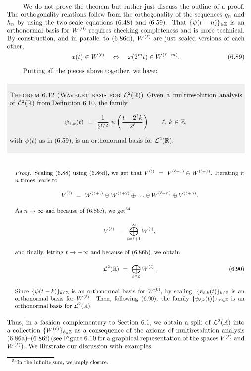
6.3. Wavelet Series 233
We do not prove the theorem but rather just discuss the outline of a proof.The orthogonality relations follow from the orthogonality of the sequences gn andhn by using the two-scale equations (6.48) and (6.59). That ψ(t − n)∈Z is anorthonormal basis for W (0) requires checking completeness and is more technical.By construction, and in parallel to (6.86d), W (ℓ) are just scaled versions of eachother,
x(t) ∈W (ℓ) ⇔ x(2mt) ∈W (ℓ−m). (6.89)
Putting all the pieces above together, we have:
Theorem 6.12 (Wavelet basis for L2(R)) Given a multiresolution analysisof L2(R) from Definition 6.10, the family
ψℓ,k(t) =1
2ℓ/2ψ
(t− 2ℓk
2ℓ
)ℓ, k ∈ Z,
with ψ(t) as in (6.59), is an orthonormal basis for L2(R).
Proof. Scaling (6.88) using (6.86d), we get that V (ℓ) = V (ℓ+1) ⊕W (ℓ+1). Iterating itn times leads to
V (ℓ) = W (ℓ+1) ⊕W (ℓ+2) ⊕ . . .⊕W (ℓ+n) ⊕ V (ℓ+n).
As n→∞ and because of (6.86c), we get54
V (ℓ) =
∞⊕
i=ℓ+1
W (i),
and finally, letting ℓ→ −∞ and because of (6.86b), we obtain
L2(R) =⊕
ℓ∈Z
W (ℓ). (6.90)
Since ψ(t − k)k∈Z is an orthonormal basis for W (0), by scaling, ψℓ,k(t)k∈Z is anorthonormal basis for W (ℓ). Then, following (6.90), the family ψℓ,k(t)ℓ,n∈Z is anorthonormal basis for L2(R).
Thus, in a fashion complementary to Section 6.1, we obtain a split of L2(R) intoa collection W (ℓ)ℓ∈Z as a consequence of the axioms of multiresolution analysis(6.86a)–(6.86f) (see Figure 6.10 for a graphical representation of the spaces V (ℓ) andW (ℓ)). We illustrate our discussion with examples.
54In the infinite sum, we imply closure.
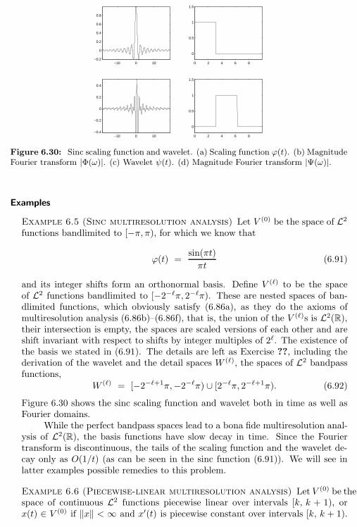
234 Chapter 6. Wavelet Bases, Frames and Transforms on Functions
−10 0 10−0.2
0
0.2
0.4
0.6
0.8
0 2 4 6 8
0
0.5
1
1.5
−10 0 10−0.4
−0.2
0
0.2
0.4
0 2 4 6 8
0
0.5
1
1.5
Figure 6.30: Sinc scaling function and wavelet. (a) Scaling function ϕ(t). (b) MagnitudeFourier transform |Φ(ω)|. (c) Wavelet ψ(t). (d) Magnitude Fourier transform |Ψ(ω)|.
Examples
Example 6.5 (Sinc multiresolution analysis) Let V (0) be the space of L2functions bandlimited to [−π, π), for which we know that
ϕ(t) =sin(πt)
πt(6.91)
and its integer shifts form an orthonormal basis. Define V (ℓ) to be the spaceof L2 functions bandlimited to [−2−ℓπ, 2−ℓπ). These are nested spaces of ban-dlimited functions, which obviously satisfy (6.86a), as they do the axioms ofmultiresolution analysis (6.86b)–(6.86f), that is, the union of the V (ℓ)s is L2(R),their intersection is empty, the spaces are scaled versions of each other and areshift invariant with respect to shifts by integer multiples of 2ℓ. The existence ofthe basis we stated in (6.91). The details are left as Exercise ??, including thederivation of the wavelet and the detail spaces W (ℓ), the spaces of L2 bandpassfunctions,
W (ℓ) = [−2−ℓ+1π,−2−ℓπ) ∪ [2−ℓπ, 2−ℓ+1π). (6.92)
Figure 6.30 shows the sinc scaling function and wavelet both in time as well asFourier domains.
While the perfect bandpass spaces lead to a bona fide multiresolution anal-ysis of L2(R), the basis functions have slow decay in time. Since the Fouriertransform is discontinuous, the tails of the scaling function and the wavelet de-cay only as O(1/t) (as can be seen in the sinc function (6.91)). We will see inlatter examples possible remedies to this problem.
Example 6.6 (Piecewise-linear multiresolution analysis) Let V (0) be thespace of continuous L2 functions piecewise linear over intervals [k, k + 1), orx(t) ∈ V (0) if ‖x‖ < ∞ and x′(t) is piecewise constant over intervals [k, k + 1).
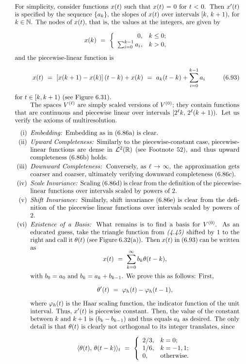
6.3. Wavelet Series 235
For simplicity, consider functions x(t) such that x(t) = 0 for t < 0. Then x′(t)is specified by the sequence ak, the slopes of x(t) over intervals [k, k + 1), fork ∈ N. The nodes of x(t), that is, the values at the integers, are given by
x(k) =
0, k ≤ 0;∑
k−1i=0 ai, k > 0,
and the piecewise-linear function is
x(t) = [x(k + 1)− x(k)] (t− k) + x(k) = ak(t− k) +k−1∑
i=0
ai (6.93)
for t ∈ [k, k + 1) (see Figure 6.31).The spaces V (ℓ) are simply scaled versions of V (0); they contain functions
that are continuous and piecewise linear over intervals [2ℓk, 2ℓ(k + 1)). Let usverify the axioms of multiresolution.
(i) Embedding: Embedding as in (6.86a) is clear.
(ii) Upward Completeness: Similarly to the piecewise-constant case, piecewise-linear functions are dense in L2(R) (see Footnote 52), and thus upwardcompleteness (6.86b) holds.
(iii) Downward Completeness: Conversely, as ℓ → ∞, the approximation getscoarser and coarser, ultimately verifying downward completeness (6.86c).
(iv) Scale Invariance: Scaling (6.86d) is clear from the definition of the piecewise-linear functions over intervals scaled by powers of 2.
(v) Shift Invariance: Similarly, shift invariance (6.86e) is clear from the defi-nition of the piecewise linear functions over intervals scaled by powers of2.
(vi) Existence of a Basis: What remains is to find a basis for V (0). As aneducated guess, take the triangle function from (4.45) shifted by 1 to theright and call it θ(t) (see Figure 6.32(a)). Then x(t) in (6.93) can be writtenas
x(t) =∞∑
k=0
bkθ(t− k),
with b0 = a0 and bk = ak + bk−1. We prove this as follows: First,
θ′(t) = ϕh(t)− ϕh(t− 1),
where ϕh(t) is the Haar scaling function, the indicator function of the unitinterval. Thus, x′(t) is piecewise constant. Then, the value of the constantbetween k and k+1 is (bk − bk−1) and thus equals ak as desired. The onlydetail is that θ(t) is clearly not orthogonal to its integer translates, since
〈θ(t), θ(t− k)〉t =
2/3, k = 0;1/6, k = −1, 1;0, otherwise.
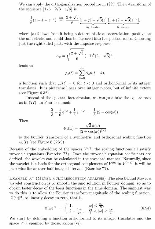
236 Chapter 6. Wavelet Bases, Frames and Transforms on Functions
We can apply the orthogonalization procedure in (??). The z-transform ofthe sequence
[1/6 2/3 1/6
]is
1
6(z + 4 + z−1)
(a)=
2 +√3
6[1 + (2 −
√3)z]︸ ︷︷ ︸
right sided
[1 + (2−√3)z−1]︸ ︷︷ ︸
left sided
,
where (a) follows from it being a deterministic autocorrelation, positive onthe unit circle, and could thus be factored into its spectral roots. Choosingjust the right-sided part, with the impulse response
αk =
√2 +√3
6(−1)k(2−
√3)k,
leads to
ϕc(t) =
∞∑
k=0
αkθ(t− k),
a function such that ϕc(t) = 0 for t < 0 and orthonormal to its integertranslates. It is piecewise linear over integer pieces, but of infinite extent(see Figure 6.32).
Instead of the spectral factorization, we can just take the square rootas in (??). In Fourier domain,
2
3+
1
6ejω +
1
6e−jω =
1
3(2 + cos(ω)).
Then,
Φs(ω) =
√3 θ(ω)
(2 + cos(ω))1/2
is the Fourier transform of a symmetric and orthogonal scaling functionϕs(t) (see Figure 6.32(c)).
Because of the embedding of the spaces V (ℓ), the scaling functions all satisfytwo-scale equations (Exercise ??). Once the two-scale equation coefficients arederived, the wavelet can be calculated in the standard manner. Naturally, sincethe wavelet is a basis for the orthogonal complement of V (0) in V (−1), it will bepiecewise linear over half-integer intervals (Exercise ??).
Example 6.7 (Meyer multiresolution analysis) The idea behind Meyer’swavelet construction is to smooth the sinc solution in Fourier domain, so as toobtain faster decay of the basis functions in the time domain. The simplest wayto do this is to allow the Fourier transform magnitude of the scaling function,|Φ(ω)|2, to linearly decay to zero, that is,
|Φ(ω)|2 =
1, |ω| < 2π
3 ;
2− 3|ω|2π ,
2π3 < |ω| < 4π
3 .(6.94)
We start by defining a function orthonormal to its integer translates and thespace V (0) spanned by those, axiom (vi).
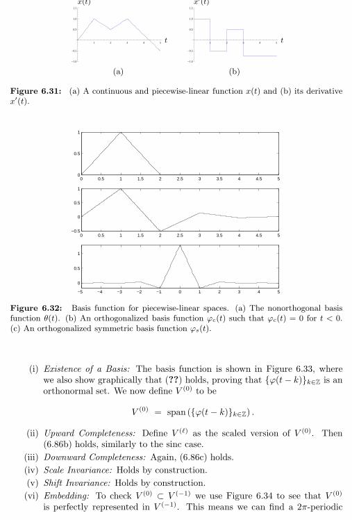
6.3. Wavelet Series 237
1 2 3 4 5
-1.0
-0.5
0.5
1.0
1.5
t
x(t)
1 2 3 4 5
-1.0
-0.5
0.5
1.0
1.5
t
x′(t)
(a) (b)
Figure 6.31: (a) A continuous and piecewise-linear function x(t) and (b) its derivativex′(t).
0 0.5 1 1.5 2 2.5 3 3.5 4 4.5 50
0.5
1
0 0.5 1 1.5 2 2.5 3 3.5 4 4.5 5−0.5
0
0.5
1
−5 −4 −3 −2 −1 0 1 2 3 4 5
0
0.5
1
Figure 6.32: Basis function for piecewise-linear spaces. (a) The nonorthogonal basisfunction θ(t). (b) An orthogonalized basis function ϕc(t) such that ϕc(t) = 0 for t < 0.(c) An orthogonalized symmetric basis function ϕs(t).
(i) Existence of a Basis: The basis function is shown in Figure 6.33, wherewe also show graphically that (??) holds, proving that ϕ(t− k)k∈Z is anorthonormal set. We now define V (0) to be
V (0) = span (ϕ(t− k)k∈Z) .
(ii) Upward Completeness: Define V (ℓ) as the scaled version of V (0). Then(6.86b) holds, similarly to the sinc case.
(iii) Downward Completeness: Again, (6.86c) holds.
(iv) Scale Invariance: Holds by construction.
(v) Shift Invariance: Holds by construction.
(vi) Embedding: To check V (0) ⊂ V (−1) we use Figure 6.34 to see that V (0)
is perfectly represented in V (−1). This means we can find a 2π-periodic
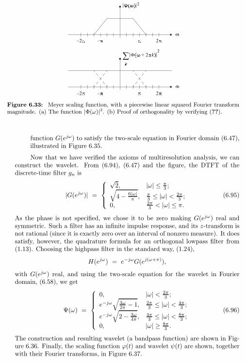
238 Chapter 6. Wavelet Bases, Frames and Transforms on Functions
Figure 6.33: Meyer scaling function, with a piecewise linear squared Fourier transformmagnitude. (a) The function |Φ(ω)|2. (b) Proof of orthogonality by verifying (??).
function G(ejω) to satisfy the two-scale equation in Fourier domain (6.47),illustrated in Figure 6.35.
Now that we have verified the axioms of multiresolution analysis, we canconstruct the wavelet. From (6.94), (6.47) and the figure, the DTFT of thediscrete-time filter gn is
|G(ejω)| =
√2, |ω| ≤ π
3 ;√4− 6|ω|
π, π
3 ≤ |ω| < 2π3 ;
0, 2π3 < |ω| ≤ π.
(6.95)
As the phase is not specified, we chose it to be zero making G(ejω) real andsymmetric. Such a filter has an infinite impulse response, and its z-transform isnot rational (since it is exactly zero over an interval of nonzero measure). It doessatisfy, however, the quadrature formula for an orthogonal lowpass filter from(1.13). Choosing the highpass filter in the standard way, (1.24),
H(ejω) = e−jωG(ej(ω+π)),
with G(ejω) real, and using the two-scale equation for the wavelet in Fourierdomain, (6.58), we get
Ψ(ω) =
0, |ω| < 2π3 ;
e−jω√
3ω2π − 1, 2π
3 ≤ |ω| < 4π3 ;
e−jω√2− 3ω
4π ,4π3 ≤ |ω| < 8π
3 ;
0, |ω| ≥ 8π3 .
(6.96)
The construction and resulting wavelet (a bandpass function) are shown in Fig-ure 6.36. Finally, the scaling function ϕ(t) and wavelet ψ(t) are shown, togetherwith their Fourier transforms, in Figure 6.37.
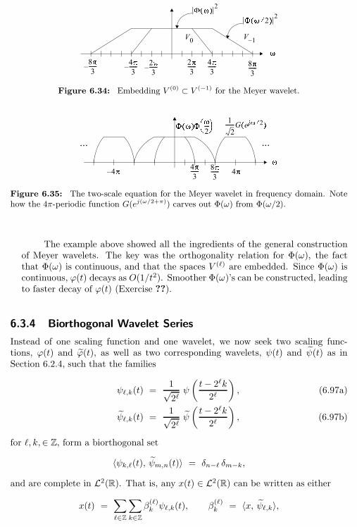
6.3. Wavelet Series 239
Figure 6.34: Embedding V (0) ⊂ V (−1) for the Meyer wavelet.
Figure 6.35: The two-scale equation for the Meyer wavelet in frequency domain. Notehow the 4π-periodic function G(ej(ω/2+π)) carves out Φ(ω) from Φ(ω/2).
The example above showed all the ingredients of the general constructionof Meyer wavelets. The key was the orthogonality relation for Φ(ω), the factthat Φ(ω) is continuous, and that the spaces V (ℓ) are embedded. Since Φ(ω) iscontinuous, ϕ(t) decays as O(1/t2). Smoother Φ(ω)’s can be constructed, leadingto faster decay of ϕ(t) (Exercise ??).
6.3.4 Biorthogonal Wavelet Series
Instead of one scaling function and one wavelet, we now seek two scaling func-tions, ϕ(t) and ϕ(t), as well as two corresponding wavelets, ψ(t) and ψ(t) as inSection 6.2.4, such that the families
ψℓ,k(t) =1√2ℓψ
(t− 2ℓk
2ℓ
), (6.97a)
ψℓ,k(t) =1√2ℓψ
(t− 2ℓk
2ℓ
), (6.97b)
for ℓ, k,∈ Z, form a biorthogonal set
〈ψk,ℓ(t), ψm,n(t)〉 = δn−ℓ δm−k,
and are complete in L2(R). That is, any x(t) ∈ L2(R) can be written as either
x(t) =∑
ℓ∈Z
∑
k∈Z
β(ℓ)kψℓ,k(t), β
(ℓ)k
= 〈x, ψℓ,k〉,
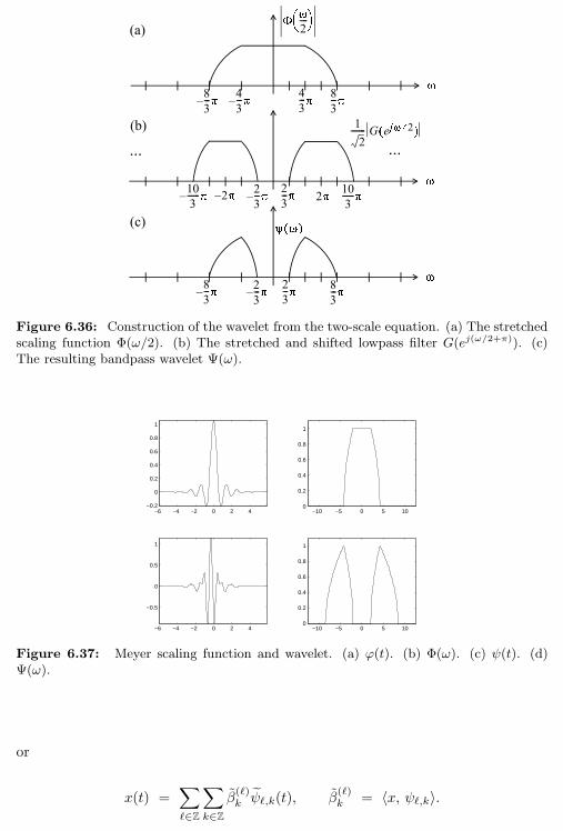
240 Chapter 6. Wavelet Bases, Frames and Transforms on Functions
Figure 6.36: Construction of the wavelet from the two-scale equation. (a) The stretchedscaling function Φ(ω/2). (b) The stretched and shifted lowpass filter G(ej(ω/2+π)). (c)The resulting bandpass wavelet Ψ(ω).
−6 −4 −2 0 2 4−0.2
0
0.2
0.4
0.6
0.8
1
−10 −5 0 5 100
0.2
0.4
0.6
0.8
1
−6 −4 −2 0 2 4
−0.5
0
0.5
1
−10 −5 0 5 100
0.2
0.4
0.6
0.8
1
Figure 6.37: Meyer scaling function and wavelet. (a) ϕ(t). (b) Φ(ω). (c) ψ(t). (d)Ψ(ω).
or
x(t) =∑
ℓ∈Z
∑
k∈Z
β(ℓ)kψℓ,k(t), β
(ℓ)k
= 〈x, ψℓ,k〉.
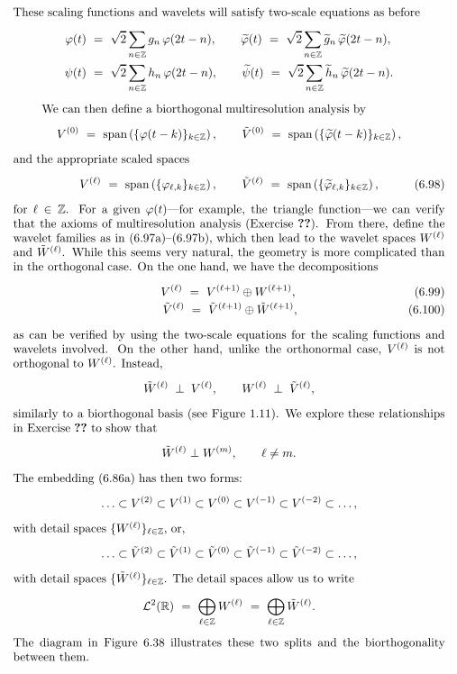
6.3. Wavelet Series 241
These scaling functions and wavelets will satisfy two-scale equations as before
ϕ(t) =√2∑
n∈Z
gn ϕ(2t− n), ϕ(t) =√2∑
n∈Z
gn ϕ(2t− n),
ψ(t) =√2∑
n∈Z
hn ϕ(2t− n), ψ(t) =√2∑
n∈Z
hn ϕ(2t− n).
We can then define a biorthogonal multiresolution analysis by
V (0) = span (ϕ(t− k)k∈Z) , V (0) = span (ϕ(t− k)k∈Z) ,
and the appropriate scaled spaces
V (ℓ) = span (ϕℓ,kk∈Z) , V (ℓ) = span (ϕℓ,kk∈Z) , (6.98)
for ℓ ∈ Z. For a given ϕ(t)—for example, the triangle function—we can verifythat the axioms of multiresolution analysis (Exercise ??). From there, define thewavelet families as in (6.97a)–(6.97b), which then lead to the wavelet spaces W (ℓ)
and W (ℓ). While this seems very natural, the geometry is more complicated thanin the orthogonal case. On the one hand, we have the decompositions
V (ℓ) = V (ℓ+1) ⊕W (ℓ+1), (6.99)
V (ℓ) = V (ℓ+1) ⊕ W (ℓ+1), (6.100)
as can be verified by using the two-scale equations for the scaling functions andwavelets involved. On the other hand, unlike the orthonormal case, V (ℓ) is notorthogonal to W (ℓ). Instead,
W (ℓ) ⊥ V (ℓ), W (ℓ) ⊥ V (ℓ),
similarly to a biorthogonal basis (see Figure 1.11). We explore these relationshipsin Exercise ?? to show that
W (ℓ) ⊥W (m), ℓ 6= m.
The embedding (6.86a) has then two forms:
. . . ⊂ V (2) ⊂ V (1) ⊂ V (0) ⊂ V (−1) ⊂ V (−2) ⊂ . . . ,
with detail spaces W (ℓ)ℓ∈Z, or,
. . . ⊂ V (2) ⊂ V (1) ⊂ V (0) ⊂ V (−1) ⊂ V (−2) ⊂ . . . ,
with detail spaces W (ℓ)ℓ∈Z. The detail spaces allow us to write
L2(R) =⊕
ℓ∈Z
W (ℓ) =⊕
ℓ∈Z
W (ℓ).
The diagram in Figure 6.38 illustrates these two splits and the biorthogonalitybetween them.
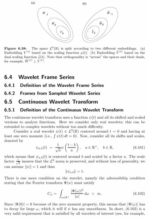
242 Chapter 6. Wavelet Bases, Frames and Transforms on Functions
Figure 6.38: The space L2(R) is split according to two different embeddings. (a)Embedding V (ℓ) based on the scaling function ϕ(t). (b) Embedding V (ℓ) based on thedual scaling function ϕ(t). Note that orthogonality is “across” the spaces and their duals,for example, W (ℓ) ⊥ V (ℓ).
6.4 Wavelet Frame Series
6.4.1 Definition of the Wavelet Frame Series
6.4.2 Frames from Sampled Wavelet Series
6.5 Continuous Wavelet Transform
6.5.1 Definition of the Continuous Wavelet Transform
The continuous wavelet transform uses a function ψ(t) and all its shifted and scaledversions to analyze functions. Here we consider only real wavelets; this can beextended to complex wavelets without too much difficulty.
Consider a real wavelet ψ(t) ∈ L2(R) centered around t = 0 and having atleast one zero moment (i.e.,
∫ψ(t) dt = 0). Now, consider all its shifts and scales,
denoted by
ψa,b(t) =1√aψ
(t− ba
), a ∈ R
+, b ∈ R, (6.101)
which means that ψa,b(t) is centered around b and scaled by a factor a. The scalefactor 1√
ainsures that the L2 norm is preserved, and without loss of generality, we
can assume ‖ψ‖ = 1 and thus‖ψa,b‖ = 1.
There is one more condition on the wavelet, namely the admissibility conditionstating that the Fourier transform Ψ(w) must satisfy
Cψ =
∫
ω∈R+
|Ψ(ω)|2|ω| dω < ∞. (6.102)
Since |Ψ(0)| = 0 because of the zero moment property, this means that |Ψ(ω)| hasto decay for large ω, which it will if ψ has any smoothness. In short, (6.102) is avery mild requirement that is satisfied by all wavelets of interest (see, for example,
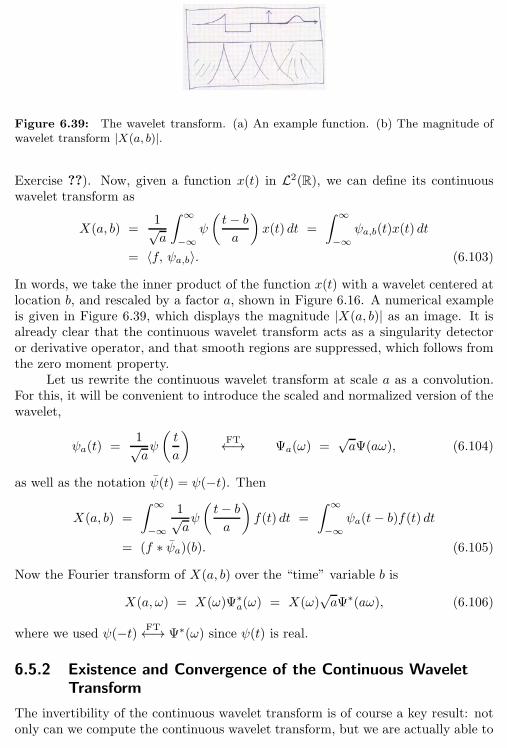
6.5. Continuous Wavelet Transform 243
Figure 6.39: The wavelet transform. (a) An example function. (b) The magnitude ofwavelet transform |X(a, b)|.
Exercise ??). Now, given a function x(t) in L2(R), we can define its continuouswavelet transform as
X(a, b) =1√a
∫ ∞
−∞ψ
(t− ba
)x(t) dt =
∫ ∞
−∞ψa,b(t)x(t) dt
= 〈f, ψa,b〉. (6.103)
In words, we take the inner product of the function x(t) with a wavelet centered atlocation b, and rescaled by a factor a, shown in Figure 6.16. A numerical exampleis given in Figure 6.39, which displays the magnitude |X(a, b)| as an image. It isalready clear that the continuous wavelet transform acts as a singularity detectoror derivative operator, and that smooth regions are suppressed, which follows fromthe zero moment property.
Let us rewrite the continuous wavelet transform at scale a as a convolution.For this, it will be convenient to introduce the scaled and normalized version of thewavelet,
ψa(t) =1√aψ
(t
a
)FT←→ Ψa(ω) =
√aΨ(aω), (6.104)
as well as the notation ψ(t) = ψ(−t). Then
X(a, b) =
∫ ∞
−∞
1√aψ
(t− ba
)f(t) dt =
∫ ∞
−∞ψa(t− b)f(t) dt
= (f ∗ ψa)(b). (6.105)
Now the Fourier transform of X(a, b) over the “time” variable b is
X(a, ω) = X(ω)Ψ∗a(ω) = X(ω)
√aΨ∗(aω), (6.106)
where we used ψ(−t) FT←→ Ψ∗(ω) since ψ(t) is real.
6.5.2 Existence and Convergence of the Continuous Wavelet
Transform
The invertibility of the continuous wavelet transform is of course a key result: notonly can we compute the continuous wavelet transform, but we are actually able to
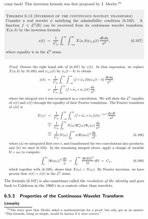
244 Chapter 6. Wavelet Bases, Frames and Transforms on Functions
come back! This inversion formula was first proposed by J. Morlet.55
Theorem 6.13 (Inversion of the continuous wavelet transform)Consider a real wavelet ψ satisfying the admissibility condition (6.102). Afunction f ∈ L2(R) can be recovered from its continuous wavelet transformX(a, b) by the inversion formula
x(t) =1
Cψ
∫ ∞
0
∫ ∞
−∞X(a, b)ψa,b(t)
db da
a2, (6.107)
where equality is in the L2 sense.
Proof. Denote the right hand side of (6.107) by x(t). In that expression, we replaceX(a, b) by (6.105) and ψa,b(t) by ψa(t− b) to obtain
x(t) =1
Cψ
∫ ∞
0
∫ ∞
−∞(f ∗ ψa)(b)ψa(t− b) db da
a2
=1
Cψ
∫ ∞
0
(f ∗ ψa ∗ ψa)(t) daa2,
where the integral over b was recognized as a convolution. We will show the L2 equalityof x(t) and x(t) through the equality of their Fourier transforms. The Fourier transformof x(t) is
X(ω) =1
Cψ
∫ ∞
−∞
∫ ∞
0
(f ∗ ψa ∗ ψa)(t)e−jωt da dta2
(a)=
1
Cψ
∫ ∞
0
X(ω)Ψ∗a(ω)Ψa(ω)
da
a2
(b)=
1
CψX(ω)
∫ ∞
0
a|Ψ(aω)|2 daa2, (6.108)
where (a) we integrated first over t, and transformed the two convolutions into products;and (b) we used (6.104). In the remaining integral above, apply a change of variableΩ = aω to compute:
∫ ∞
0
|Ψ(aω)|2 daa
=
∫ ∞
0
|Ψ(Ω)|2Ω
dΩ = Cψ, (6.109)
which together with (6.108), shows that X(ω) = X(ω). By Fourier inversion, we haveproven that x(t) = x(t) in the L2 sense.
The formula (6.107) is also sometimes called the resolution of the identity and goesback to Calderon in the 1960’s in a context other than wavelets.
6.5.3 Properties of the Continuous Wavelet Transform
Linearity
55The story goes that Morlet asked a mathematician for a proof, but only got as an answer:“This formula, being so simple, would be known if it were correct.”
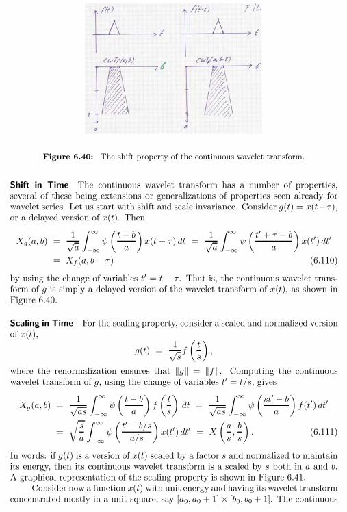
6.5. Continuous Wavelet Transform 245
Figure 6.40: The shift property of the continuous wavelet transform.
Shift in Time The continuous wavelet transform has a number of properties,several of these being extensions or generalizations of properties seen already forwavelet series. Let us start with shift and scale invariance. Consider g(t) = x(t−τ),or a delayed version of x(t). Then
Xg(a, b) =1√a
∫ ∞
−∞ψ
(t− ba
)x(t− τ) dt =
1√a
∫ ∞
−∞ψ
(t′ + τ − b
a
)x(t′) dt′
= Xf (a, b− τ) (6.110)
by using the change of variables t′ = t − τ . That is, the continuous wavelet trans-form of g is simply a delayed version of the wavelet transform of x(t), as shown inFigure 6.40.
Scaling in Time For the scaling property, consider a scaled and normalized versionof x(t),
g(t) =1√sf
(t
s
),
where the renormalization ensures that ‖g‖ = ‖f‖. Computing the continuouswavelet transform of g, using the change of variables t′ = t/s, gives
Xg(a, b) =1√as
∫ ∞
−∞ψ
(t− ba
)f
(t
s
)dt =
1√as
∫ ∞
−∞ψ
(st′ − ba
)f(t′) dt′
=
√s
a
∫ ∞
−∞ψ
(t′ − b/sa/s
)x(t′) dt′ = X
(a
s,b
s
). (6.111)
In words: if g(t) is a version of x(t) scaled by a factor s and normalized to maintainits energy, then its continuous wavelet transform is a scaled by s both in a and b.A graphical representation of the scaling property is shown in Figure 6.41.
Consider now a function x(t) with unit energy and having its wavelet transformconcentrated mostly in a unit square, say [a0, a0 + 1]× [b0, b0 + 1]. The continuous
246 Chapter 6. Wavelet Bases, Frames and Transforms on Functions
Figure 6.41: The scaling property of the continuous wavelet transform.
wavelet transform of g(t) is then mostly concentrated in a square [sa0, s(a0 + 1)]×[sb0, s(b0+1)], a cell of area s2. But remember that g(t) has still unit energy, whileits continuous wavelet transform now covers a surface increased by s2. Therefore,when evaluating an energy measure in the continuous wavelet transform domain,we need to renormalize by a factor a2, as was seen in both the inversion formula(6.107) and the energy conservation formula (6.112).
When comparing the above properties with the equivalent ones from waveletseries, the major difference is that shift and scale are arbitrary real variables, ratherthan constrained, dyadic rationals (powers of 2 for the scale, multiples of the scalefor shifts). Therefore, we obtain true time scale and shift properties.
Parseval’s Equality Closely related to the resolution of the identity is an energyconservation formula, an analogue to Parseval’s equality.
Theorem 6.14 (Energy conservation of the continuous wavelet transform)Consider a function f ∈ L2(R) and its continuous wavelet transform X(a, b) withrespect to a real wavelet ψ satisfying the admissibility condition (6.102). Then,the following energy conservation holds:
∫ ∞
−∞|x(t)|2 dt =
1
Cψ
∫
a∈R+
∫
b∈R
|X(a, b)|2 db da
a2. (6.112)
6.5. Continuous Wavelet Transform 247
Proof. Expand the right hand side (without the leading constant) as∫
a∈R+
∫
b∈R
|X(a, b)|2 db da
a2(a)=
∫
a∈R+
∫
b∈R
∣∣(f ∗ ψa)(b)∣∣2 db da
a2
(b)=
∫
a∈R+
1
2π
∫
b∈R
∣∣X(ω)√aΨ∗(aω)
∣∣2 dω daa2
=
∫
a∈R+
1
2π
∫
b∈R
|X(ω)|2 |Ψ(aω)|2 dω daa,
where (a) uses (6.105); and (b) uses Parseval’s equality for the Fourier transform withrespect to b, also transforming the convolution into a product. Changing the order ofintegration and in (c) using the change of variables Ω = aω allows us to write the aboveas
∫
a∈R+
∫
b∈R
|X(a, b)|2 db da
a2=
∫ ∞
−∞
1
2π|X(ω)|2
∫
a∈R+
|Ψ(aω)| daa2
dω
(c)=
∫
ω∈R
1
2π|F (ω)|2
∫
ω∈R+
|Ψ(Ω)|2 dΩ
Ω︸ ︷︷ ︸
Cψ
dω.
Therefore1
Cψ
∫
a∈R+
∫
b∈R
|X(a, b)|2 db da
a2=
1
2π
∫
ω∈R
|X(ω)|2 dω,
and applying Parseval’s equality to the right side proves (6.112).
Both the inversion formula and the energy conservation formula use da db/a2
as an integration measure. This is related to the scaling property of the continuouswavelet transform as will be shown below. Note that the extension to a complexwavelet is not hard; the integral over da has to go from −∞ to ∞, and Cψ has tobe defined accordingly.
Redundancy The continuous wavelet transform maps a one-dimensional functioninto a two-dimensional one: this is clearly very redundant. In other words, onlya small subset of two-dimensional functions correspond to wavelet transforms. Weare thus interested in characterizing the image of one-dimensional functions in thecontinuous wavelet transform domain.
A simple analogue is in order. Consider an M by N matrix T having or-thonormal columns (i.e., T TT = I) with M > N . Suppose y is the image of anarbitrary vector x ∈ RN through the operator T , or y = Tx. Clearly y belongs toa subspace S of RM , namely the span of the columns of T .
There is a simple test to check if an arbitrary vector z ∈ RM belongs to S.Introduce the kernel matrix K,
K = TT T , (6.113)
which is the M by M matrix of outer products of the columns of T . Then, a vectorz belong to S if and only if it satisfies
Kz = z. (6.114)
248 Chapter 6. Wavelet Bases, Frames and Transforms on Functions
Indeed, if z is in S, then it can be written as z = Tx for some x. Substituting thisinto the left side of (6.114) leads to
Kz = TT TTx = Tx = z.
Conversely, if (6.114) holds then z = Kz = TT Tz = Tx, showing that z belongs toS.
If z is not in S, then Kz = z is the orthogonal projection of z onto S ascan be verified. See Exercise ?? for a discussion of this, as well as the case ofnon-orthonormal columns in T .
We now extend the test given in (6.114) to the case of the continuous wavelettransform. For this, let us introduce the reproducing kernel of the wavelet ψ(t),defined as
K(a0, b0, a, b) = 〈ψa0,b0 , ψa,b〉. (6.115)
This is the deterministic crosscorrelation of two wavelets at scale and shifts (a0, b0)and (a, b), respectively, and is the equivalent of the matrix K in (6.113).
Call V the space of functions X(a, b) that are square integrable with respectto the measure (db da)/a2 (see also Theorem 6.14). In this space, there exists asubspace S that corresponds to bona fide continuous wavelet transforms. Similarlyto what we just did in finite dimensions, we give a test to check whether a functionX(a, b) in V actually belongs to S, that is, if it is the continuous wavelet transformof some one-dimensional function x(t).
Theorem 6.15 (Reproducing kernel property of the continuous wavelet transform)A function X(a, b) is the continuous wavelet transform of a function x(t) if andonly if it satisfies
X(a0, b0) =1
Cψ
∫ ∞
0
∫ ∞
−∞K(a0, b0, a, b)X(a, b)
db da
a2. (6.116)
Proof. We show that if X(a, b) is a continuous wavelet transform of some function x(t),then (6.116) holds. Completing the proof by showing that the converse is also true isleft as Exercise ??.
By assumption,
X(a0, b0) =
∫ ∞
−∞ψa0,b0(t)x(t)dt.
Replace x(t) by its inversion formula (6.107), or
F (a0, b0) =
∫ ∞
−∞ψa0,b0(t)
1
Cψ
∫ ∞
0
∫ ∞
−∞ψa,b(t)X(a, b)
db da
a2dt
(a)=
1
Cψ
∫ ∞
0
∫ ∞
−∞
∫ ∞
−∞ψa0,b0(t)ψa,b(t)X(a, b) dt
db da
a2
(b)=
1
Cψ
∫ ∞
0
∫ ∞
−∞K(a0, b0, a, b)X(a, b)
db da
a2,
where (a) we interchanged the order of integration; and (b) we integrated over t to getthe reproducing kernel (6.115).
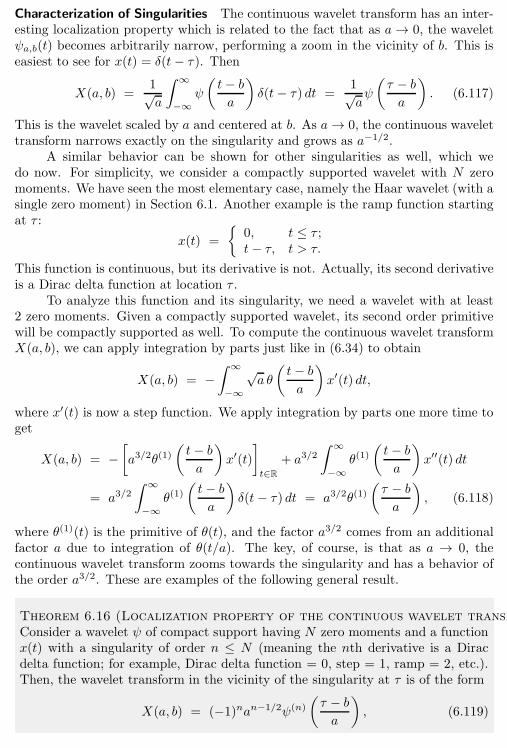
6.5. Continuous Wavelet Transform 249
Characterization of Singularities The continuous wavelet transform has an inter-esting localization property which is related to the fact that as a→ 0, the waveletψa,b(t) becomes arbitrarily narrow, performing a zoom in the vicinity of b. This iseasiest to see for x(t) = δ(t− τ). Then
X(a, b) =1√a
∫ ∞
−∞ψ
(t− ba
)δ(t− τ) dt =
1√aψ
(τ − ba
). (6.117)
This is the wavelet scaled by a and centered at b. As a→ 0, the continuous wavelettransform narrows exactly on the singularity and grows as a−1/2.
A similar behavior can be shown for other singularities as well, which wedo now. For simplicity, we consider a compactly supported wavelet with N zeromoments. We have seen the most elementary case, namely the Haar wavelet (with asingle zero moment) in Section 6.1. Another example is the ramp function startingat τ :
x(t) =
0, t ≤ τ ;t− τ, t > τ.
This function is continuous, but its derivative is not. Actually, its second derivativeis a Dirac delta function at location τ .
To analyze this function and its singularity, we need a wavelet with at least2 zero moments. Given a compactly supported wavelet, its second order primitivewill be compactly supported as well. To compute the continuous wavelet transformX(a, b), we can apply integration by parts just like in (6.34) to obtain
X(a, b) = −∫ ∞
−∞
√a θ
(t− ba
)x′(t) dt,
where x′(t) is now a step function. We apply integration by parts one more time toget
X(a, b) = −[a3/2θ(1)
(t− ba
)x′(t)
]
t∈R
+ a3/2∫ ∞
−∞θ(1)
(t− ba
)x′′(t) dt
= a3/2∫ ∞
−∞θ(1)
(t− ba
)δ(t− τ) dt = a3/2θ(1)
(τ − ba
), (6.118)
where θ(1)(t) is the primitive of θ(t), and the factor a3/2 comes from an additionalfactor a due to integration of θ(t/a). The key, of course, is that as a → 0, thecontinuous wavelet transform zooms towards the singularity and has a behavior ofthe order a3/2. These are examples of the following general result.
Theorem 6.16 (Localization property of the continuous wavelet transform)Consider a wavelet ψ of compact support having N zero moments and a functionx(t) with a singularity of order n ≤ N (meaning the nth derivative is a Diracdelta function; for example, Dirac delta function = 0, step = 1, ramp = 2, etc.).Then, the wavelet transform in the vicinity of the singularity at τ is of the form
X(a, b) = (−1)nan−1/2ψ(n)
(τ − ba
), (6.119)
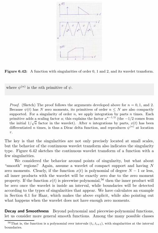
250 Chapter 6. Wavelet Bases, Frames and Transforms on Functions
Figure 6.42: A function with singularities of order 0, 1 and 2, and its wavelet transform.
where ψ(n) is the nth primitive of ψ.
Proof. (Sketch) The proof follows the arguments developed above for n = 0, 1, and 2.Because ψ(t) has N zero moments, its primitives of order n ≤ N are also compactlysupported. For a singularity of order n, we apply integration by parts n times. Eachprimitive adds a scaling factor a; this explains the factor an−1/2 (the −1/2 comes fromthe initial 1/
√a factor in the wavelet). After n integrations by parts, x(t) has been
differentiated n times, is thus a Dirac delta function, and reproduces ψ(n) at locationτ .
The key is that the singularities are not only precisely located at small scales,but the behavior of the continuous wavelet transform also indicates the singularitytype. Figure 6.42 sketches the continuous wavelet transform of a function with afew singularities.
We considered the behavior around points of singularity, but what about“smooth” regions? Again, assume a wavelet of compact support and having Nzero moments. Clearly, if the function x(t) is polynomial of degree N − 1 or less,all inner products with the wavelet will be exactly zero due to the zero momentproperty. If the function x(t) is piecewise polynomial,56 then the inner product willbe zero once the wavelet is inside an interval, while boundaries will be detectedaccording to the types of singularities that appear. We have calculates an examplein Section 6.1 for Haar, which makes the above explicit, while also pointing outwhat happens when the wavelet does not have enough zero moments.
Decay and Smoothness Beyond polynomial and piecewise-polynomial functions,let us consider more general smooth functions. Among the many possible classes
56That is, the function is a polynomial over intervals (ti, ti+1), with singularities at the intervalboundaries.
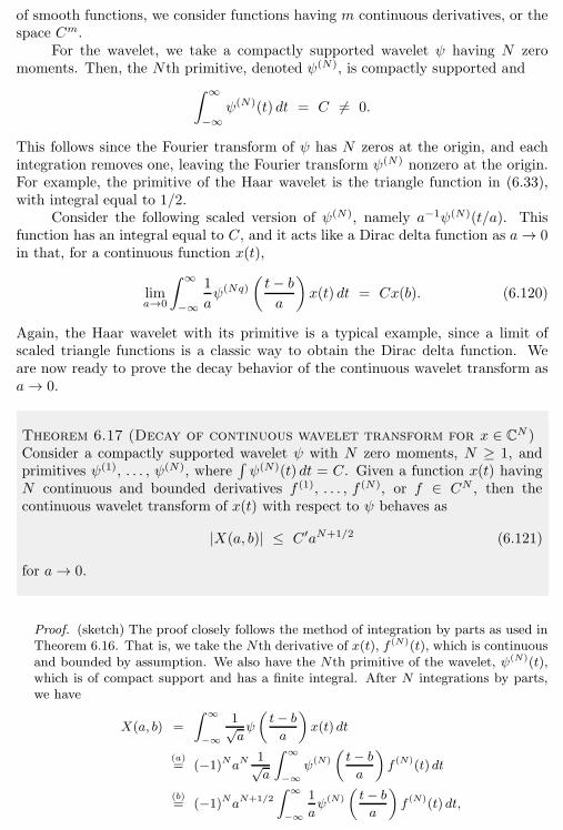
6.5. Continuous Wavelet Transform 251
of smooth functions, we consider functions having m continuous derivatives, or thespace Cm.
For the wavelet, we take a compactly supported wavelet ψ having N zeromoments. Then, the Nth primitive, denoted ψ(N), is compactly supported and
∫ ∞
−∞ψ(N)(t) dt = C 6= 0.
This follows since the Fourier transform of ψ has N zeros at the origin, and eachintegration removes one, leaving the Fourier transform ψ(N) nonzero at the origin.For example, the primitive of the Haar wavelet is the triangle function in (6.33),with integral equal to 1/2.
Consider the following scaled version of ψ(N), namely a−1ψ(N)(t/a). Thisfunction has an integral equal to C, and it acts like a Dirac delta function as a→ 0in that, for a continuous function x(t),
lima→0
∫ ∞
−∞
1
aψ(Nq)
(t− ba
)x(t) dt = Cx(b). (6.120)
Again, the Haar wavelet with its primitive is a typical example, since a limit ofscaled triangle functions is a classic way to obtain the Dirac delta function. Weare now ready to prove the decay behavior of the continuous wavelet transform asa→ 0.
Theorem 6.17 (Decay of continuous wavelet transform for x ∈ CN)Consider a compactly supported wavelet ψ with N zero moments, N ≥ 1, andprimitives ψ(1), . . . , ψ(N), where
∫ψ(N)(t) dt = C. Given a function x(t) having
N continuous and bounded derivatives f (1), . . . , f (N), or f ∈ CN , then thecontinuous wavelet transform of x(t) with respect to ψ behaves as
|X(a, b)| ≤ C′aN+1/2 (6.121)
for a→ 0.
Proof. (sketch) The proof closely follows the method of integration by parts as used inTheorem 6.16. That is, we take the Nth derivative of x(t), f (N)(t), which is continuousand bounded by assumption. We also have the Nth primitive of the wavelet, ψ(N)(t),which is of compact support and has a finite integral. After N integrations by parts,we have
X(a, b) =
∫ ∞
−∞
1√aψ
(t− ba
)x(t) dt
(a)= (−1)NaN 1√
a
∫ ∞
−∞ψ(N)
(t− ba
)f (N)(t) dt
(b)= (−1)NaN+1/2
∫ ∞
−∞
1
aψ(N)
(t− ba
)f (N)(t) dt,
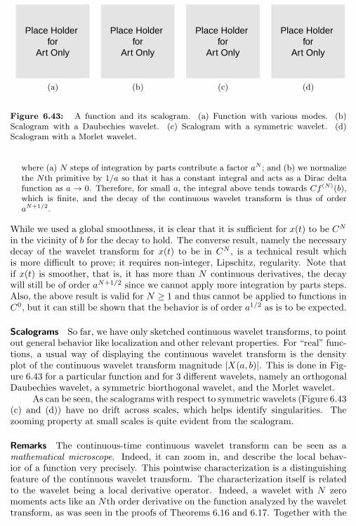
252 Chapter 6. Wavelet Bases, Frames and Transforms on Functions
Place Holder for
Art Only
Place Holder for
Art Only
Place Holder for
Art Only
Place Holder for
Art Only
(a) (b) (c) (d)
Figure 6.43: A function and its scalogram. (a) Function with various modes. (b)Scalogram with a Daubechies wavelet. (c) Scalogram with a symmetric wavelet. (d)Scalogram with a Morlet wavelet.
where (a) N steps of integration by parts contribute a factor aN ; and (b) we normalizethe Nth primitive by 1/a so that it has a constant integral and acts as a Dirac deltafunction as a → 0. Therefore, for small a, the integral above tends towards Cf (N)(b),which is finite, and the decay of the continuous wavelet transform is thus of orderaN+1/2.
While we used a global smoothness, it is clear that it is sufficient for x(t) to be CN
in the vicinity of b for the decay to hold. The converse result, namely the necessarydecay of the wavelet transform for x(t) to be in CN , is a technical result whichis more difficult to prove; it requires non-integer, Lipschitz, regularity. Note thatif x(t) is smoother, that is, it has more than N continuous derivatives, the decaywill still be of order aN+1/2 since we cannot apply more integration by parts steps.Also, the above result is valid for N ≥ 1 and thus cannot be applied to functions inC0, but it can still be shown that the behavior is of order a1/2 as is to be expected.
Scalograms So far, we have only sketched continuous wavelet transforms, to pointout general behavior like localization and other relevant properties. For “real” func-tions, a usual way of displaying the continuous wavelet transform is the densityplot of the continuous wavelet transform magnitude |X(a, b)|. This is done in Fig-ure 6.43 for a particular function and for 3 different wavelets, namely an orthogonalDaubechies wavelet, a symmetric biorthogonal wavelet, and the Morlet wavelet.
As can be seen, the scalograms with respect to symmetric wavelets (Figure 6.43(c) and (d)) have no drift across scales, which helps identify singularities. Thezooming property at small scales is quite evident from the scalogram.
Remarks The continuous-time continuous wavelet transform can be seen as amathematical microscope. Indeed, it can zoom in, and describe the local behav-ior of a function very precisely. This pointwise characterization is a distinguishingfeature of the continuous wavelet transform. The characterization itself is relatedto the wavelet being a local derivative operator. Indeed, a wavelet with N zeromoments acts like an Nth order derivative on the function analyzed by the wavelettransform, as was seen in the proofs of Theorems 6.16 and 6.17. Together with the
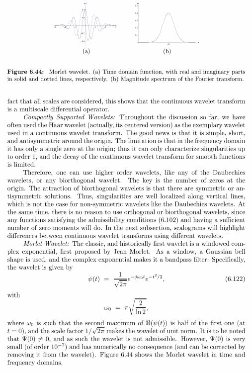
6.5. Continuous Wavelet Transform 253
-3 -2 -1 1 2 3t
-0.4
-0.2
0.2
0.4
psi
w0w
0.1
0.2
0.3
0.4
0.5Psi
(a) (b)
Figure 6.44: Morlet wavelet. (a) Time domain function, with real and imaginary partsin solid and dotted lines, respectively. (b) Magnitude spectrum of the Fourier transform.
fact that all scales are considered, this shows that the continuous wavelet transformis a multiscale differential operator.
Compactly Supported Wavelets: Throughout the discussion so far, we haveoften used the Haar wavelet (actually, its centered version) as the exemplary waveletused in a continuous wavelet transform. The good news is that it is simple, short,and antisymmetric around the origin. The limitation is that in the frequency domainit has only a single zero at the origin; thus it can only characterize singularities upto order 1, and the decay of the continuous wavelet transform for smooth functionsis limited.
Therefore, one can use higher order wavelets, like any of the Daubechieswavelets, or any biorthogonal wavelet. The key is the number of zeros at theorigin. The attraction of biorthogonal wavelets is that there are symmetric or an-tisymmetric solutions. Thus, singularities are well localized along vertical lines,which is not the case for non-symmetric wavelets like the Daubechies wavelets. Atthe same time, there is no reason to use orthogonal or biorthogonal wavelets, sinceany functions satisfying the admissibility conditions (6.102) and having a sufficientnumber of zero moments will do. In the next subsection, scalograms will highlightdifferences between continuous wavelet transforms using different wavelets.
Morlet Wavelet: The classic, and historically first wavelet is a windowed com-plex exponential, first proposed by Jean Morlet. As a window, a Gaussian bellshape is used, and the complex exponential makes it a bandpass filter. Specifically,the wavelet is given by
ψ(t) =1√2πe−jω0te−t
2/2, (6.122)
with
ω0 = π
√2
ln 2,
where ω0 is such that the second maximum of ℜ(ψ(t)) is half of the first one (att = 0), and the scale factor 1/
√2π makes the wavelet of unit norm. It is to be noted
that Ψ(0) 6= 0, and as such the wavelet is not admissible. However, Ψ(0) is verysmall (of order 10−7) and has numerically no consequence (and can be corrected byremoving it from the wavelet). Figure 6.44 shows the Morlet wavelet in time andfrequency domains.
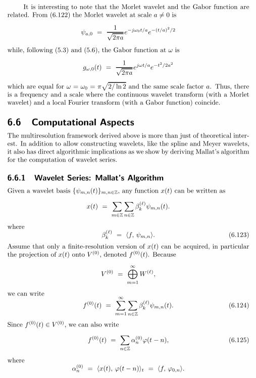
254 Chapter 6. Wavelet Bases, Frames and Transforms on Functions
It is interesting to note that the Morlet wavelet and the Gabor function arerelated. From (6.122) the Morlet wavelet at scale a 6= 0 is
ψa,0 =1√2πa
e−jω0t/ae−(t/a)2/2
while, following (5.3) and (5.6), the Gabor function at ω is
gω,0(t) =1√2πa
ejωt/ae−t2/2a2
which are equal for ω = ω0 = π√2/ ln 2 and the same scale factor a. Thus, there
is a frequency and a scale where the continuous wavelet transform (with a Morletwavelet) and a local Fourier transform (with a Gabor function) coincide.
6.6 Computational Aspects
The multiresolution framework derived above is more than just of theoretical inter-est. In addition to allow constructing wavelets, like the spline and Meyer wavelets,it also has direct algorithmic implications as we show by deriving Mallat’s algorithmfor the computation of wavelet series.
6.6.1 Wavelet Series: Mallat’s Algorithm
Given a wavelet basis ψm,n(t)m,n∈Z, any function x(t) can be written as
x(t) =∑
m∈Z
∑
n∈Z
β(ℓ)kψm,n(t).
whereβ(ℓ)k
= 〈f, ψm,n〉. (6.123)
Assume that only a finite-resolution version of x(t) can be acquired, in particularthe projection of x(t) onto V (0), denoted f (0)(t). Because
V (0) =
∞⊕
m=1
W (ℓ),
we can write
f (0)(t) =
∞∑
m=1
∑
n∈Z
β(ℓ)kψm,n(t). (6.124)
Since f (0)(t) ∈ V (0), we can also write
f (0)(t) =∑
n∈Z
α(0)nϕ(t − n), (6.125)
whereα(0)n
= 〈x(t), ϕ(t− n)〉t = 〈f, ϕ0,n〉.

6.6. Computational Aspects 255
Given these two ways of expressing f (0)(t), how to go from one to the other? Theanswer, as to be expected, lies in the two-scale equation, and leads to a filter bankalgorithm. Consider f (1)(t), the projection of f (0)(t) onto V (1). This involvescomputing the inner products
α(1)n
= 〈f (0)(t), 1√2ϕ(t/2− n)〉t, n ∈ Z. (6.126)
From (6.48), we can write
1√2ϕ(t/2− n) =
∑
k∈Z
gkϕ(t− 2n− k). (6.127)
Replacing this and (6.125) into (6.126) leads to
α(1)n
=∑
k∈Z
∑
ℓ∈Z
gkα(0)ℓ〈ϕ(t− 2n− k), ϕ(t− ℓ)〉t
(a)=∑
ℓ∈Z
gℓ−2nα(0)ℓ
(b)= (g ∗ α(0))2n, (6.128)
where (a) follows because the inner product is 0 unless ℓ = 2n+ k; and (b) simplyrewrites the sum as a convolution, with
gn = g−n.
The upshot is that the sequence α(1)n is obtained from convolving α
(0)n with g (the
time-reversed impulse response of g) and downsampling by 2. The same develop-ment for the wavelet series coefficients
β(1)k
= 〈f (0)(t), 1√2ψ(t/2− n)〉t
yields
β(1)k
= (h ∗ α(0))2n, (6.129)
wherehn = h−n
is the time-reversed impulse response of the highpass filter h. The argument justdeveloped holds irrespectively of the scale at which we start, thus allowing to split afunction f (ℓ) in V (ℓ) into its components f (m+1) in V (m+1) and d(m+1) in W (m+1).This split is achieved by filtering and downsampling α(ℓ) with g and h, respectively.Likewise, this process can be iterated k times, to go from V (ℓ) to V (m+k), whilesplitting off W (m+1), W (m+2), . . . , W (m+k), or
V (ℓ) = W (m+1) ⊕W (m+1) ⊕ . . .⊕W (m+k) ⊕ V (m+k).
The key insight is of course that once we have an initial projection, for exam-
ple, f (0)(t) with expansion coefficients α(0)n , then all the other expansion coefficients
can be computed using discrete-time filtering. This is shown in Figure 6.46, where
the sequence α(0)n , corresponding to an initial projection of x(t) onto V (0), is decom-
posed into the expansion coefficients in W (1), W (2), W (3) and V (3). This algorithmis known as Mallat’s algorithm, since it is directly related to the multiresolutionanalysis of Mallat and Meyer.
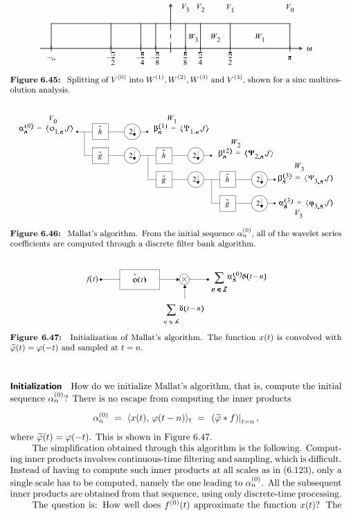
256 Chapter 6. Wavelet Bases, Frames and Transforms on Functions
Figure 6.45: Splitting of V (0) intoW (1),W (2),W (3) and V (3), shown for a sinc multires-olution analysis.
Figure 6.46: Mallat’s algorithm. From the initial sequence α(0)n , all of the wavelet series
coefficients are computed through a discrete filter bank algorithm.
Figure 6.47: Initialization of Mallat’s algorithm. The function x(t) is convolved withϕ(t) = ϕ(−t) and sampled at t = n.
Initialization How do we initialize Mallat’s algorithm, that is, compute the initial
sequence α(0)n ? There is no escape from computing the inner products
α(0)n
= 〈x(t), ϕ(t− n)〉t = (ϕ ∗ f)|t=n ,
where ϕ(t) = ϕ(−t). This is shown in Figure 6.47.The simplification obtained through this algorithm is the following. Comput-
ing inner products involves continuous-time filtering and sampling, which is difficult.Instead of having to compute such inner products at all scales as in (6.123), only a
single scale has to be computed, namely the one leading to α(0)n . All the subsequent
inner products are obtained from that sequence, using only discrete-time processing.The question is: How well does f (0)(t) approximate the function x(t)? The
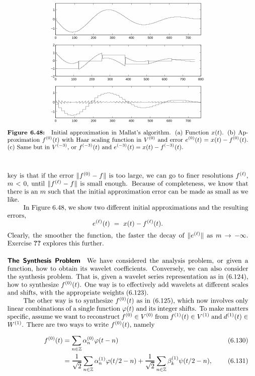
6.6. Computational Aspects 257
0 100 200 300 400 500 600 700
−1
0
1
0 100 200 300 400 500 600 700 800−2
−1
0
1
2
0 100 200 300 400 500 600 700
−1
0
1
Figure 6.48: Initial approximation in Mallat’s algorithm. (a) Function x(t). (b) Ap-proximation f (0)(t) with Haar scaling function in V (0) and error e(0)(t) = x(t) − f (0)(t).(c) Same but in V (−3), or f (−3)(t) and e(−3)(t) = x(t)− f (−3)(t).
key is that if the error ‖f (0) − f‖ is too large, we can go to finer resolutions f (ℓ),m < 0, until ‖f (ℓ) − f‖ is small enough. Because of completeness, we know thatthere is an m such that the initial approximation error can be made as small as welike.
In Figure 6.48, we show two different initial approximations and the resultingerrors,
e(ℓ)(t) = x(t) − f (ℓ)(t).
Clearly, the smoother the function, the faster the decay of ‖e(ℓ)‖ as m → −∞.Exercise ?? explores this further.
The Synthesis Problem We have considered the analysis problem, or given afunction, how to obtain its wavelet coefficients. Conversely, we can also considerthe synthesis problem. That is, given a wavelet series representation as in (6.124),how to synthesize f (0)(t). One way is to effectively add wavelets at different scalesand shifts, with the appropriate weights (6.123).
The other way is to synthesize f (0)(t) as in (6.125), which now involves onlylinear combinations of a single function ϕ(t) and its integer shifts. To make mattersspecific, assume we want to reconstruct f (0) ∈ V (0) from f (1)(t) ∈ V (1) and d(1)(t) ∈W (1). There are two ways to write f (0)(t), namely
f (0)(t) =∑
n∈Z
α(0)nϕ(t− n) (6.130)
=1√2
∑
n∈Z
α(1)nϕ(t/2− n) + 1√
2
∑
n∈Z
β(1)kψ(t/2− n), (6.131)
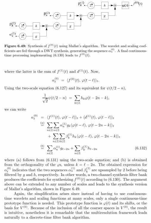
258 Chapter 6. Wavelet Bases, Frames and Transforms on Functions
Figure 6.49: Synthesis of f (0)(t) using Mallat’s algorithm. The wavelet and scaling coef-
ficients are fed through a DWT synthesis, generating the sequence α(0)n . A final continuous-
time processing implementing (6.130) leads to f (0)(t).
where the latter is the sum of f (1)(t) and d(1)(t). Now,
α(0)ℓ
= 〈f (0)(t), ϕ(t− ℓ)〉t.
Using the two-scale equation (6.127) and its equivalent for ψ(t/2− n),1√2ψ(t/2− n) =
∑
k∈Z
hkϕ(t− 2n− k),
we can write
α(0)ℓ
= 〈f (1)(t), ϕ(t− ℓ)〉t + 〈d(1)(t), ϕ(t− ℓ)〉t(a)=∑
n∈Z
∑
n∈Z
α(1)ngk〈ϕ(t − ℓ), ϕ(t− 2n− k)〉t
+∑
n∈Z
∑
k∈Z
β(1)khk〈ϕ(t− ℓ), ϕ(t− 2n− k)〉t
(b)=∑
n∈Z
α(1)ngℓ−2n +
∑
n∈Z
β(1)khℓ−2n (6.132)
where (a) follows from (6.131) using the two-scale equation; and (b) is obtainedfrom the orthogonality of the ϕs, unless k = ℓ − 2n. The obtained expression for
α(0)ℓ
indicates that the two sequences α(1)n and β
(1)k
are upsampled by 2 before beingfiltered by g and h, respectively. In other words, a two-channel synthesis filter bankproduces the coefficients for synthesizing f (0)(t) according to (6.130). The argumentabove can be extended to any number of scales and leads to the synthesis versionof Mallat’s algorithm, shown in Figure 6.49.
Again, the simplification arises since instead of having to use continuous-time wavelets and scaling functions at many scales, only a single continuous-timeprototype function is needed. This prototype function is ϕ(t) and its shifts, or thebasis for V (0). Because of the inclusion of all the coarser spaces in V (0), the resultis intuitive, nonetheless it is remarkable that the multiresolution framework leadsnaturally to a discrete-time filter bank algorithm.
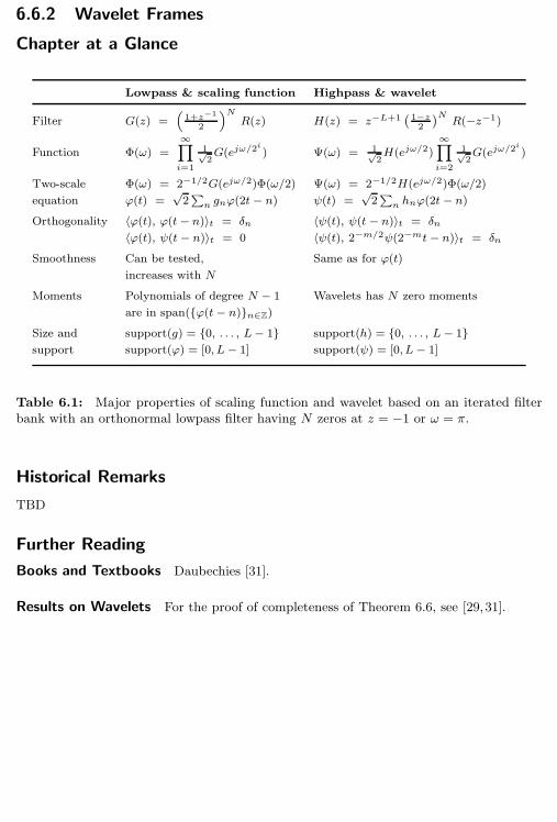
Chapter at a Glance 259
6.6.2 Wavelet Frames
Chapter at a Glance
Lowpass & scaling function Highpass & wavelet
Filter G(z) =(
1+z−1
2
)NR(z) H(z) = z−L+1
(1−z2
)NR(−z−1)
Function Φ(ω) =∞∏
i=1
1√2G(ejω/2
i
) Ψ(ω) = 1√2H(ejω/2)
∞∏
i=2
1√2G(ejω/2
i
)
Two-scale Φ(ω) = 2−1/2G(ejω/2)Φ(ω/2) Ψ(ω) = 2−1/2H(ejω/2)Φ(ω/2)
equation ϕ(t) =√2∑n gnϕ(2t − n) ψ(t) =
√2∑n hnϕ(2t − n)
Orthogonality 〈ϕ(t), ϕ(t − n)〉t = δn 〈ψ(t), ψ(t − n)〉t = δn
〈ϕ(t), ψ(t − n)〉t = 0 〈ψ(t), 2−m/2ψ(2−mt − n)〉t = δn
Smoothness Can be tested, Same as for ϕ(t)
increases with N
Moments Polynomials of degree N − 1 Wavelets has N zero moments
are in span(ϕ(t − n)n∈Z)
Size and support(g) = 0, . . . , L− 1 support(h) = 0, . . . , L− 1support support(ϕ) = [0, L− 1] support(ψ) = [0, L− 1]
Table 6.1: Major properties of scaling function and wavelet based on an iterated filterbank with an orthonormal lowpass filter having N zeros at z = −1 or ω = π.
Historical Remarks
TBD
Further Reading
Books and Textbooks Daubechies [31].
Results on Wavelets For the proof of completeness of Theorem 6.6, see [29,31].
Bibliography
[1] T. Aach. New criteria for shift variance and wide-sense cyclostationarity inmultirate filter banks. In Proc. IEEE Int. Workshop on Spectral Methods andMultirate Signal Proc., pages 7–13, Florence, Italy, 2006.
[2] T. Aach. Comparative analysis of shift variance and cyclostationarity in mul-tirate filter banks. IEEE Trans. Circ. and Syst., 54(5):1077–1087, May 2007.
[3] N. I. Akhiezer and I. M. Glazman. Theory of Linear Operators in HilbertSpaces, volume 1. Frederick Ungar Publishing, 1966.
[4] S. Akkarakaran and P. P. Vaidyanathan. Bifrequency and bispectrum maps:A new look at multirate systems with stochastic inputs. IEEE Trans. SignalProc., 48(3):723–736, March 2000.
[5] M. Antonini, M. Barlaud, P. Mathieu, and I. Daubechies. Image coding usingwavelet transform. IEEE Trans. Image Proc., 1(2):205–220, April 1992.
[6] P. Auscher. Wavelets: Mathematics and Applications, chapter Remarks onthe local Fourier bases, pages 203–218. CRC Press, 1994.
[7] M. G. Bellanger and J. L. Daguet. TDM-FDM transmultiplexer: Digitalpolyphase and FFT. IEEE Trans. Commun., 22(9):1199–1204, September1974.
[8] J. J. Benedetto and M. C. Fickus. Finite normalized tight frames. Adv. Comp.Math., sp. iss. Frames, 18:357–385, 2003.
[9] B. G. Bodmann, P. G. Casazza, and G. Kutyniok. A quantitative notionof redundancy for finite frames. In Journ. Appl. and Comput. HarmonicAnalysis, 2010.
[10] H. Bolcskei and F. Hlawatsch. Gabor Analysis and Algorithms: Theory andApplications, chapter Oversampled modulated filter banks, pages 295–322.Birkhauser, Boston, MA, 1998.
[11] H. Bolcskei and F. Hlawatsch. Oversampled cosine modulated filter bankswith perfect reconstruction. IEEE Trans. Circ. and Syst. II: Analog andDigital Signal Proc., 45(8):1057–1071, August 1998.
265

266 Bibliography
[12] H. Bolcskei, F. Hlawatsch, and H. G. Feichtinger. Frame-theoretic analysisof oversampled filter banks. IEEE Trans. Signal Proc., 46(12):3256–3269,December 1998.
[13] A. P. Bradley. Shift invariance in the discrete wavelet transform. In Proc.Digit. Image Comp., December 2003.
[14] A. A. M. L. Bruckens and A. W. M. van den Enden. New networks for perfectinversion and perfect reconstruction. IEEE Journ. Sel. Areas in Commun.,10(1), September 1992.
[15] P. J. Burt and E. H. Adelson. The Laplacian pyramid as a compact imagecode. IEEE Trans. Commun., 31(4):532–540, April 1983.
[16] E. J. Candes. Curvelet Web Site. http://www.curvelet.org/papers.html.
[17] E. J. Candes, L. Demanet, D. L. Donoho, and L. Ying. Fast discrete curvelettransforms. Preprint, 2005.
[18] P. G. Casazza. The art of frame theory. Taiwanese Journ. Math., 4(2):129–202, 2000.
[19] P. G. Casazza and J. Kovacevic. Equal-norm tight frames with erasures. Adv.Comp. Math., sp. iss. Frames, 18:387–430, 2002.
[20] P. G. Casazza and G. Kutyniok. A generalization of Gram-Schmidt orthogo-nalization generating all Parseval frames. Adv. Comp. Math., 27:65–78, 2007.Preprint.
[21] A. Chebira and J. Kovacevic. Lapped tight frame transforms. In Proc. IEEEInt. Conf. Acoust., Speech and Signal Proc., volume III, pages 857–860, Hon-olulu, HI, April 2007.
[22] O. Christensen. An Introduction to Frames and Riesz Bases. Birkhauser,2002.
[23] A. Cohen, I. Daubechies, and J.-C. Feauveau. Biorthogonal bases of compactlysupported wavelets. Commun. Pure and Appl. Math., 45:485–560, 1992.
[24] R. R. Coifman, Y. Meyer, S. Quake, and M. V. Wickerhauser. Signal pro-cessing and compression with wavelet packets. Technical report, Yale Univ.,1991.
[25] A. L. Cunha, J. Zhou, and M. N. Do. The nonsubsampled contourlettransform: Theory, design, and applications. IEEE Trans. Image Proc.,15(10):3089–3101, October 2006.
[26] Z. Cvetkovic. Oversampled modulated filter banks and tight Gabor framesin ℓ2(Z). In Proc. IEEE Int. Conf. Acoust., Speech and Signal Proc., pages1456–1459, Detroit, MI, May 1995.
Bibliography 267
[27] Z. Cvetkovic and M. Vetterli. Oversampled filter banks. IEEE Trans. SignalProc., 46(5):1245–1255, May 1998.
[28] Z. Cvetkovic and M. Vetterli. Tight Weyl-Heisenberg frames in ℓ2(Z). IEEETrans. Signal Proc., 46(5):1256–1259, May 1998.
[29] I. Daubechies. Orthonormal bases of compactly supported wavelets. Commun.Pure and Appl. Math., 41:909–996, November 1988.
[30] I. Daubechies. The wavelet transform, time-frequency localization and signalanalysis. IEEE Trans. Inform. Th., 36(5):961–1005, September 1990.
[31] I. Daubechies. Ten Lectures on Wavelets. SIAM, Philadelphia, PA, 1992.
[32] I. Daubechies, A. Grossman, and Y. Meyer. Painless nonorthogonal expan-sions. Journ. Math. Phys., 27:1271–1283, November 1986.
[33] M. N. Do and M. Vetterli. The finite ridgelet transform for image represen-tation. IEEE Trans. Image Proc., 12(1):16–28, January 2003.
[34] M. N. Do and M. Vetterli. The contourlet transform: An efficient directionalmultiresolution image representation. IEEE Trans. Image Proc., 14(12):2091–2106, December 2005.
[35] E. Dubois. The sampling and reconstruction of time-varying imagery withapplication in video systems. Proc. IEEE, 73(4):502–522, April 1985.
[36] R. J. Duffin and A. C. Schaeffer. A class of nonharmonic Fourier series. Trans.Amer. Math. Soc., 72:341–366, 1952.
[37] Y. Eldar and H. Bolcskei. Geometrically uniform frames. IEEE Trans. Inform.Th., 49(4):993–1006, April 2003.
[38] D. Esteban and C. Galand. Applications of quadrature mirror filters to splitband voice coding schemes. In Proc. IEEE Int. Conf. Acoust., Speech andSignal Proc., pages 191–195, 1995.
[39] H. G. Feichtinger and T. Strohmer, editors. Gabor Analysis and Algorithms:Theory and Applications. Birkhauser, Boston, MA, 1998.
[40] D. Gabor. Theory of communication. Journ. IEE, 93:429–457, 1946.
[41] V. K. Goyal, M. Vetterli, and N. T. Thao. Quantized overcomplete expan-sions in RN : Analysis, synthesis, and algorithms. IEEE Trans. Inform. Th.,44(1):16–31, January 1998.
[42] D. Han and D. R. Larson. Frames, bases and group representations. Number697 in Memoirs AMS. AMS Press, Providence, RI, 2000.
[43] C. Heil and D. Walnut. Continuous and discrete wavelet transforms. SIAMReview, 31:628–666, 1989.
268 Bibliography
[44] C. Herley and M. Vetterli. Biorthogonal bases of symmetric compactly sup-ported wavelets. In M. Farge and et al., editors, Proc. Wavelets, Fractals andFourier Transforms. Oxford Univ. Press, 1991.
[45] C. Herley and M. Vetterli. Wavelets and recursive filter banks. IEEE Trans.Signal Proc., August 1993.
[46] C. Herley and M. Vetterli. Orthogonal time-varying filter banks and waveletpackets. IEEE Trans. Signal Proc., 42(10):2650–2663, October 1994.
[47] O. Herrmann. On the approximation problem in nonrecursive digital filterdesign. IEEE Trans. Circ. Theory, 18:411–413, 1971.
[48] R. B. Holmes and V. I. Paulsen. Optimal frames for erasures. Linear Algebraand Its Appl., 377:31–51, 2004.
[49] J. D. Johnston. A filter family designed for use in Quadrature Mirror FilterBanks. In Proc. IEEE Int. Conf. Acoust., Speech and Signal Proc., pages291–294, Denver, CO, 1980.
[50] G. Karlsson and M. Vetterli. Theory of two - dimensional multirate filterbanks. IEEE Trans. Acoust., Speech, and Signal Proc., 38(6):925–937, June1990.
[51] N. G. Kingsbury. The dual-tree complex wavelet transform: A new efficienttool for image restoration and enhancement. In Proc. Eur. Signal Proc. Conf.,pages 319–322, 1998.
[52] N. G. Kingsbury. Image processing with complex wavelets. Phil. Trans. RoyalSoc. London A, September 1999.
[53] N. G. Kingsbury. Complex wavelets for shift invariant analysis and filtering ofsignals. Journ. Appl. and Comput. Harmonic Analysis, 10(3):234–253, May2001.
[54] J. Kovacevic and A. Chebira. An Introduction to Frames. Foundations andTrends in Signal Proc. Now Publishers, 2008.
[55] J. Kovacevic and M. Vetterli. Nonseparable multidimensional perfect recon-struction filter banks and wavelet bases forRn . IEEE Trans. Inform. Th., sp.iss. Wavelet Transforms and Multiresolution Signal Analysis, 38(2):533–555,March 1992. Chosen for inclusion in Fundamental Papers in Wavelet Theory.
[56] D. Labate, W-Q. Lim, G. Kutyniok, and G. Weiss. Sparse multidimensionalrepresentation using shearlets. In Proc. SPIE Conf. Wavelet Appl. in Signaland Image Proc., pages 254–262, Bellingham, WA, 2005.
[57] D. J. LeGall and A. Tabatabai. Subband coding of digital images using sym-metric short kernel filters and arithmetic coding techniques. In Proc. IEEEInt. Conf. Acoust., Speech and Signal Proc., pages 761–765, New York, NY,1988.
Bibliography 269
[58] Y. Lu and M. N. Do. The finer directional wavelet transform. In Proc.IEEE Int. Conf. Acoust., Speech and Signal Proc., volume 4, pages 573–576,Philadelphia, PA, March 2005.
[59] S. Mallat. Multiresolution approximations and wavelet orthonormal bases ofL2(R). Trans. Amer. Math. Soc., 315:69–87, September 1989.
[60] S. Mallat. A Wavelet Tour of Signal Processing. Academic Press, secondedition, 1999.
[61] H. S. Malvar. Signal Processing with Lapped Transforms. Artech House,Norwood, MA, 1992.
[62] T. G. Marshall. U-L block-triangular matrix and ladder realizations of sub-band codes. In Proc. IEEE Int. Conf. Acoust., Speech and Signal Proc.,volume 3, pages 177–180, 1993.
[63] J. L. Massey and T. Mittelholzer. Sequences II: Methods in Communication,Security and Computer Sciences, chapter Welch’s bound and sequence setsfor code-division multiple-access systems, pages 63–78. Springer-Verlag, NewYork, NY, 1993.
[64] F. Mintzer. Filters for distortion-free two-band multirate filter banks. IEEETrans. Acoust., Speech, and Signal Proc., 33(3):626–630, June 1985.
[65] I. Newton. Opticks or A Treatise of the Reflections, Refractions, Inflectionsand Colours of Light. Royal Society, 1703.
[66] H. J. Nussbaumer. Complex quadrature mirror filters. In Proc. IEEE Int.Conf. Acoust., Speech and Signal Proc., volume II, pages 221–223, Boston,MA, 1983.
[67] B. Porat. Digital Processing of Random Signals. Prentice Hall, EnglewoodCliffs, NJ, 1994.
[68] B. Porat. A Course in Digital Signal Processing. John Wiley & Sons, NewYork, NY, 1996.
[69] K. Ramchandran and M. Vetterli. Best wavelet packet bases in a rate-distortion sense. IEEE Trans. Image Proc., 2(2):160–175, April 1993.
[70] T. A. Ramstad. IIR filter bank for subband coding of images. In Proc. IEEEInt. Symp. Circ. and Syst., pages 827–830, 1988.
[71] J. M. Renes, R. Blume-Kohout, A. J. Scot, and C. M. Caves. Symmet-ric informationally complete quantum measurements. Journ. Math. Phys.,45(6):2171–2180, 2004.
[72] O. Rioul. A discrete-time multiresolution theory. IEEE Trans. Signal Proc.,41(8):2591–2606, August 1993.
270 Bibliography
[73] O. Rioul and P. Duhamel. Fast algorithms for discrete and continuous wavelettransforms. IEEE Trans. Inform. Th., sp. iss. Wavelet Transforms and Mul-tiresolution Signal Analysis, 38(2):569–586, March 1992.
[74] N. Saito and R. R. Coifman. Local discriminant bases. In Proc. SPIE Conf.Vis. Commun. and Image Proc., pages 2–14, 1994.
[75] N. Saito and R. R. Coifman. Local discriminant bases and their applications.Journ. Math. Imag. Vis., 5:337–358, 1995.
[76] A. Sandryhaila, A. Chebira, C. Milo, J. Kovacevic, and M. Puschel. System-atic construction of real lapped tight frame transforms. IEEE Trans. SignalProc., 58(5):2256–2567, May 2010.
[77] I. W. Selesnick. Wavelets in Signal and Image Analysis, chapter The doubledensity DWT. Kluwer Academic Publishers, 2001.
[78] I. W. Selesnick. The double-density dual-tree DWT. IEEE Trans. SignalProc., 52(5):1304–1314, May 2004.
[79] I. Shah and T. A. C. M. Kalker. On ladder structures and linear phaseconditions for bi-orthogonal filter banks. In Proc. IEEE Int. Conf. Acoust.,Speech and Signal Proc., pages 181–184, 1994.
[80] E. P. Simoncelli. Simoncelli Web Site.http://www.cns.nyu.edu/∼eero/steerpyr/.
[81] E. P. Simoncelli, W. T. Freeman, E. H. Adelson, and D. J. Heeger. Shiftablemultiscale transforms. IEEE Trans. Inform. Th., sp. iss. Wavelet Transformsand Multiresolution Signal Analysis, 38(2):587–607, March 1992.
[82] M. J. T. Smith. IIR analysis/synthesis systems, chapter in Subband ImageCoding. Kluwer Academic Press, Boston, MA, 1991. J. W. Woods ed.
[83] M. J. T. Smith and T. P. Barnwell III. Exact reconstruction for tree-structuredsubband coders. IEEE Trans. Acoust., Speech, and Signal Proc., 34(3):431–441, June 1986.
[84] A. K. Soman, P. P. Vaidyanathan, and T. Q. Nguyen. Linear phase parauni-tary filter banks: Theory, factorizations and applications. IEEE Trans. SignalProc., sp. iss. Wavelets and Signal Proc., 41(12), December 1993.
[85] J.-L. Starck, M. Elad, and D. L. Donoho. Redundant multiscale transformsand their application for morphological component separation. Advances inImaging and Electron Physics, 132, 2004.
[86] P. Stoica and R. Moses. Introduction to Spectral Analysis. Prentice Hall,Englewood Cliffs, NJ, 2000.
[87] G. Strang and T. Nguyen. Wavelets and Filter Banks. Wellesley CambridgePress, Boston, MA, 1996.
Bibliography 271
[88] T. Strohmer. Modern Sampling Theory: Mathematics and Applications, chap-ter Finite and infinite-dimensional models for oversampled filter banks, pages297–320. Birkhauser, Boston, MA, 2000.
[89] T. Strohmer and R. Heath. Grassmannian frames with applications to cod-ing and communications. Journ. Appl. and Comput. Harmonic Analysis,14(3):257–175, 2003.
[90] W. Sweldens. The lifting scheme: A custom-design construction of biorthog-onal wavelets. Journ. Appl. and Comput. Harmonic Analysis, 1996.
[91] C. W. Therrien. Issues in multirate statistical signal processing. In Proc.Asilomar Conf. Signal, Syst. and Comp., volume 1, pages 573–576, PacificGrove, CA, 2001.
[92] J. A. Tropp, I. S. Dhillon, R. W. Heath, Jr., and T. Strohmer. Designingstructured tight frames via an alternating projection method. IEEE Trans.Inform. Th., 51(1):188–209, January 2005.
[93] M. K. Tsatsanis and G. B. Giannakis. Principal component filter banks foroptimal multiresolution analysis. IEEE Trans. Signal Proc., 43(8):1766–1777,August 1995.
[94] M. Unser. An extension of the Karhunen-Loeve transform for wavelets andperfect reconstruction filterbanks. In Proc. SPIE Conf. Wavelet Appl. inSignal and Image Proc., volume 2034, pages 45–56, San Diego, CA, July1993.
[95] M. Unser. Wavelets, filterbanks, and the Karhunen-Loeve transform. In Proc.Eur. Conf. Signal Proc., volume III, pages 1737–1740, Rhodes, Greece, 1998.
[96] P. P. Vaidyanathan. Quadrature mirror filter banks, M-band extensions andperfect reconstruction techniques. IEEE Acoust., Speech, and Signal Proc.Mag., 4(3):4–20, July 1987.
[97] P. P. Vaidyanathan. Theory and design of M-channel maximally decimatedquadrature mirror filters with arbitrary M, having the perfect reconstructionproperty. IEEE Trans. Acoust., Speech, and Signal Proc., 35(4):476–492, April1987.
[98] P. P. Vaidyanathan. Multirate Systems and Filter Banks. Prentice Hall,Englewood Cliffs, NJ, 1992.
[99] P. P. Vaidyanathan and S. Akkarakaran. A review of the theory and ap-plications of principal component filter banks. Journ. Appl. and Comput.Harmonic Analysis, 10(3):254–289, May 2001.
[100] P. P. Vaidyanathan and P.-Q. Hoang. Lattice structures for optimal designand robust implementation of two-channel perfect reconstruction filter banks.IEEE Trans. Acoust., Speech, and Signal Proc., 36(1):81–94, January 1988.

272 Bibliography
[101] P. P. Vaidyanathan and Z. Doganata. The role of lossless systems in mod-ern digital signal processing: A tutorial. IEEE Trans. Educ., 32(3):181–197,August 1989.
[102] R. Vale and S. Waldron. Tight frames and their symmetries. Const. Approx.,21:83–112, 2005.
[103] M. Vetterli. Filter banks allowing perfect reconstruction. Signal Proc.,10(3):219–244, April 1986.
[104] M. Vetterli. A theory of multirate filter banks. IEEE Trans. Acoust., Speech,and Signal Proc., 35(3):356–372, March 1987.
[105] M. Vetterli and C. Herley. Wavelets and filter banks: Theory and design.IEEE Trans. Signal Proc., 40(9):2207–2232, September 1992.
[106] M. Vetterli and J. Kovacevic. Wavelets and Subband Coding.Signal Processing. Prentice Hall, Englewood Cliffs, NJ, 1995.http://waveletsandsubbandcoding.org/.
[107] M. Vetterli, J. Kovacevic, and V. K. Goyal. Foundations of Signal Processing.Cambridge Univ. Press, 2013.
[108] M. Vetterli and D. J. LeGall. Perfect reconstruction FIR filter banks: Someproperties and factorizations. IEEE Trans. Acoust., Speech, and Signal Proc.,37(7):1057–1071, July 1989.
[109] E. Viscito and J. P. Allebach. The analysis and design of multidimensionalFIR perfect reconstruction filter banks for arbitrary sampling lattices. IEEETrans. Circ. and Syst., 38(1):29–42, January 1991.
[110] P. Viswanath and V. Anantharam. Optimal sequences and sum capacity ofsynchronous CDMA systems. IEEE Trans. Inform. Th., 45(6):1984–1991,September 1999.
[111] S. Waldron. Generalised Welch bound equality sequences are tight frames.IEEE Trans. Inform. Th., 49(9):2307–2309, September 2003.
[112] M. V. Wickerhauser. INRIA lectures on wavelet packet algorithms. Technicalreport, Yale Univ., March 1991.
[113] M. V. Wickerhauser. Lectures on wavelet packet algorithms, 1992.