BOSTON UNIVERSITY

GRADUATE SCHOOL OF ARTS AND SCIENCES

Thesis

BIOME LEVEL CLASSIFICATION OF LAND COVER AT

CONTINENTAL SCALES USING DECISION TREES

by

ALEXANDER LOTSCH

Vordiplom, Free University of Berlin, 1996

Submitted in partial ful�llment of the

requirements for the degree of

Master of Arts

1999

Approved by

First ReaderMark Friedl, Ph.D.Assistant Professor of Geography

Second ReaderRanga Myneni, Ph.D.Associate Professor of Geography

Third ReaderSucharita Gopal, Ph.D.Associate Professor of Geography

Acknowledgments

I would like to thank the people at the Department of Geography at Boston Univer-

sity, who made my time as a graduate student a rewarding and enriching experience.

Particular thanks goes to Mark Friedl, who guided me through this thesis with dedi-

cation and an extraordinary combination of rigour, exibility and academic support.

His attitude and openness helped foster a fruitful atmosphere, that enhanced my

academic experience. I would like to thank Ranga Myneni, who initially encouraged

me to pursue a degree in physical geography. He provided me the �nancial and

academic opportunity to integrate and participate in on-going research, which gave

me many critical insights. Also, I am grateful for the academic advice I received

from Sucharita Gopal. I especially appreciate her holistic view on geography, which

provided me orientation at several stages of my studies.

Many things I achieved during the two years in the Department of Geography were

only possible with the support of other graduate students. I am especially grateful to

Doug McIver, who has been extremely helpful throughout my thesis and coursework.

Many thanks to all my o�ce-mates, who assisted me numerous times with computer

problems and John Hodges for his imaginary support.

Finally, I would like to express my sincere gratitude to Chung Yi Lung for her

patience, advice and unyielding support as well as the German Fulbright Commission,

which funded my �rst year and allowed me to broaden my horizons in many ways.

iii

BIOME LEVEL CLASSIFICATION OF LAND COVER AT

CONTINENTAL SCALES USING DECISION TREES

ALEXANDER LOTSCH

Abstract

Land cover plays a key role in terrestrial biogeochemical processes. There-

fore many problems require accurate information on the distribution and prop-

erties of land cover. A decision tree classi�cation algorithm is used to generate

a land cover map of North America from remotely sensed data with 1 km

resolution in a 6-biome classi�cation scheme. To do this, the normalized di�er-

ence vegetation index (NDVI) data from the Advanced Very High Resolution

Radiometer (AVHRR) is used in association with ancillary data sources. Train-

ing sites required for this approach were generated by the Boston University

Land Cover and Land-Cover Change Research Group and improved in �ve pre-

processing steps. Accuracy assessment of the map produced via decision tree

classi�cation yields a site-based map accuracy of 73%. The map is compared

with maps generated from the same data, but classi�ed using the International

Geosphere Biosphere Program (IGBP) classi�cation scheme. Biome classes are

mapped with approximately 5% higher overall accuracies than IGBP classes.

The biome map will be useful for remote sensing-based retrievals of leaf area

index (LAI) and the fraction of absorbed photosynthetically active radiation

(FAPAR).

iv

Contents

1 Introduction 1

2 Background 5

2.1 The Role of Land Cover in Biogeochemical Modeling . . . . . . . . . 5

2.2 Global Land Cover Classi�cation Approaches . . . . . . . . . . . . . . 7

2.2.1 Conventional Approaches . . . . . . . . . . . . . . . . . . . . . 7

2.2.2 Remote Sensing-Based Approaches . . . . . . . . . . . . . . . 8

2.2.3 Biome-Based Classi�cation . . . . . . . . . . . . . . . . . . . . 11

2.3 Radiative Transfer Modeling of Vegetation Canopies . . . . . . . . . . 13

2.4 Tree-Based Classi�cation Algorithms . . . . . . . . . . . . . . . . . . 17

3 Methodology 21

3.1 Land Cover Classi�cation Algorithms . . . . . . . . . . . . . . . . . . 21

3.1.1 Data . . . . . . . . . . . . . . . . . . . . . . . . . . . . . . . . 22

3.1.2 Site Data Extraction and Classi�cation Estimation . . . . . . 23

3.1.3 Decision Tree Parameters . . . . . . . . . . . . . . . . . . . . 27

3.2 Cross-Walking from IGBP Classes to Biomes . . . . . . . . . . . . . . 29

3.3 Comparison of UMD, EDC and BU Maps . . . . . . . . . . . . . . . 31

3.4 Accuracy Assessment . . . . . . . . . . . . . . . . . . . . . . . . . . . 33

3.5 Improving Training Data Quality . . . . . . . . . . . . . . . . . . . . 37

v

4 Results 39

4.1 Classi�cation Performance . . . . . . . . . . . . . . . . . . . . . . . . 39

4.1.1 IGBP Scheme . . . . . . . . . . . . . . . . . . . . . . . . . . . 41

4.1.2 Biome Scheme . . . . . . . . . . . . . . . . . . . . . . . . . . . 46

4.2 Comparison between Classi�cation Schemes . . . . . . . . . . . . . . 52

4.3 Map Comparisons . . . . . . . . . . . . . . . . . . . . . . . . . . . . . 53

4.3.1 Accuracy Coe�cients for the UMD and EDC Maps . . . . . . 53

4.3.2 Pixel-Based Comparisons . . . . . . . . . . . . . . . . . . . . . 56

5 Discussion 60

5.1 Training Data Improvement . . . . . . . . . . . . . . . . . . . . . . . 60

5.2 IGBP Classi�cation Performance . . . . . . . . . . . . . . . . . . . . 65

5.3 Biome-Level Classi�cation Performance . . . . . . . . . . . . . . . . . 67

5.4 Separability of Land Cover Classes . . . . . . . . . . . . . . . . . . . 68

5.5 Map Comparison . . . . . . . . . . . . . . . . . . . . . . . . . . . . . 70

6 Conclusions 71

A Appendix 85

vi

List of Tables

1 Visible, red, near-infrared (NIR) and shortwave infrared bands (SWIR)

for AVHRR and MODIS . . . . . . . . . . . . . . . . . . . . . . . . . 11

2 Canopy structural attributes of global land covers from the viewpoint

of radiative transfer modeling . . . . . . . . . . . . . . . . . . . . . . 16

3 Comparison of the IGBP and biome classi�cation scheme . . . . . . . 30

4 Recoded UMD classes . . . . . . . . . . . . . . . . . . . . . . . . . . 32

5 Arrangement of reference and test data in a confusion matrix . . . . . 34

6 Overview of site-based classi�cation performance improvement . . . . 41

7 Errors of omission for selected classes in the IGBP scheme. . . . . . . 43

8 Errors of commission for selected classes in the IGBP scheme. . . . . 44

9 Error matrix for biome classes and site-based accuracy coe�cients for

the uncleaned training data set (I). . . . . . . . . . . . . . . . . . . . 47

10 Error matrix for biome classes and site-based accuracy coe�cients for

the cleaned data set (II). . . . . . . . . . . . . . . . . . . . . . . . . . 48

11 Error matrix for biome classes and site-based accuracy coe�cients us-

ing SLCR labels (III). . . . . . . . . . . . . . . . . . . . . . . . . . . 49

12 Error matrix for biome classes and site-based accuracy coe�cients with

additional training sites (IV). . . . . . . . . . . . . . . . . . . . . . . 50

vii

13 Error matrix for biome classes and site-based accuracy coe�cients for

proportional sampling (V). . . . . . . . . . . . . . . . . . . . . . . . . 51

14 Test of signi�cant di�erences between accuracy coe�cients . . . . . . 52

15 Accuracy coe�cients for aggregated IGBP maps into a 7-class scheme. 53

16 Error matrix and site-based accuracy coe�cients for the UMD map in

the IGBP scheme. . . . . . . . . . . . . . . . . . . . . . . . . . . . . . 54

17 Error matrix and site-based accuracy coe�cients for the EDC map in

the IGBP scheme. . . . . . . . . . . . . . . . . . . . . . . . . . . . . . 55

18 Error matrix and site-based accuracy coe�cients for the UMD map in

the biome scheme. . . . . . . . . . . . . . . . . . . . . . . . . . . . . 56

19 Error matrix and site-based accuracy coe�cients for the EDC map in

the biome scheme. . . . . . . . . . . . . . . . . . . . . . . . . . . . . 57

20 Frequency of classes in the IGBP scheme for the UMD, EDC and BU

maps. . . . . . . . . . . . . . . . . . . . . . . . . . . . . . . . . . . . 58

21 Frequency of classes in the biome scheme for the UMD, EDC and BU

maps. . . . . . . . . . . . . . . . . . . . . . . . . . . . . . . . . . . . 59

22 Overall agreement of the UMD, EDC and BU maps in the IGBP and

biome classi�cation scheme. . . . . . . . . . . . . . . . . . . . . . . . 59

23 IGBP class de�nitions . . . . . . . . . . . . . . . . . . . . . . . . . . 85

24 Error matrix for IGBP classes and site-based accuracy coe�cients for

the uncleaned training data set (I). . . . . . . . . . . . . . . . . . . . 86

viii

25 Error matrix for IGBP classes and site-based accuracy coe�cients for

the cleaned data set (II). . . . . . . . . . . . . . . . . . . . . . . . . . 87

26 Error matrix for IGBP classes and site-based accuracy coe�cients us-

ing SLCR labels (III) . . . . . . . . . . . . . . . . . . . . . . . . . . . 88

27 Error matrix for IGBP classes and site-based accuracy coe�cients with

additional training sites (IV). . . . . . . . . . . . . . . . . . . . . . . 89

28 Error matrix for IGBP classes and site-based accuracy coe�cients for

proportional sampling (V). . . . . . . . . . . . . . . . . . . . . . . . . 90

29 Pixel-based comparison of UMD and BU maps in the IGBP scheme. . 91

30 Pixel-based comparison of UMD and EDC maps in the IGBP scheme. 92

31 Pixel-based comparison of BU and EDC maps in the IGBP scheme. . 93

32 Pixel-based comparison of UMD and EDC maps in the biome scheme. 94

33 Pixel-based comparison of UMD and BU maps in the biome scheme. . 95

34 Pixel-based comparison of BU and EDC maps in the biome scheme. . 96

ix

List of Figures

1 Relationships of NDVI/LAI and NDVI/FAPAR . . . . . . . . . . . . 14

2 Decision tree structure . . . . . . . . . . . . . . . . . . . . . . . . . . 19

3 Data processing ow . . . . . . . . . . . . . . . . . . . . . . . . . . . 25

4 Examples of multivariate statistical outliers. . . . . . . . . . . . . . . 26

5 Supervised classi�cation of IGBP classes for North America. . . . . . 97

6 Supervised classi�cation of biome classes for North America. . . . . . 98

7 Map comparison in the biome scheme between EDC and BU. . . . . . 99

8 Map comparison in the biome scheme between UMD and BU. . . . . 100

x

List of Abbreviations

AVHRR Advanced Very High Resolution Radiometer

BU Boston University

CART Classi�cation and Regression Tree

DAAC Distributed Active Archive Center

EROS Earth Resources Observation System

EDC EROS Data Center

EOS Earth Observing System

ET Evapo-Transpiration

FAPAR Fraction of Absorbed Photosynthetically Active Radiation

GLCC Global Land Cover Characterization

IGBP International Geosphere Biosphere Program

IR Infra-Red

ISG Integerized Sinosoidal Grid

LAI Leaf Area Index

LUT Look-Up Table

MISR Multiangle Imaging Spectroradiometer

MODIS Moderate Imaging Spectroradiometer

MLRC Multiresolution Land Characterization

xi

NASA National Aeronautics Space Administration

NIR Near-Infrared

NDVI Normalized Di�erence Vegetation Index

NPP Net Primary Productivity

NOAA National Oceanic and Atmospheric Administration

POLDER Polarization and Directionality of Earth's Re ectances

RTM Radiative Transfer Model

SLCR Seasonal Land Cover Regions

SPOT Systeme Probatoire d`Observation de la Terre

SVI Spectral Vegetation Index

SWIR Shortwave Infra-Red

TM Thematic Mapper

UMD University of Maryland, College Park

UTM Universe Transverse Mercator

xii

1 Introduction

Land cover plays a key role in terrestrial biogeochemical processes and is related in

a number of ways to the dynamics of global climate. Further, changes in land cover

induced by human activity have profound implications for climate, the functioning of

ecosystems, and biogeochemical uxes at regional and global scales [Lean and War-

ilow 1989; Dickinson and Henderson-Sellers 1988]. As a consequence, a wide range of

problems require reliable and accurate information on global land cover, most impor-

tantly the distribution and properties of vegetation. Mapping techniques from the

remote sensing domain are superior to conventional ground-based methods of vegeta-

tion mapping [Townshend et al. 1991]. The data source most commonly used in the

mapping of global vegetation cover is the Advanced Very High Resolution Radiometer

(AVHRR) with a spatial resolution of 1.1 km at nadir. In particular, the normalized

di�erence vegetation index (NDVI) has been used to map vegetation as well as to

infer the amount of photosynthetically active vegetation on the ground [Tucker 1979].

With the implementation of NASA's Earth Observing System (NASA-EOS) a

new generation of satellite data will be available for scienti�c research. The Moderate

Resolution Imaging Spectroradiometer (MODIS) is expected to provide substantially

better data for future land cover mapping [Justice et al. 1998]. Further, the Multi-

Angle Imaging Spectroradiometer (MISR) will obtain multiple view angles on the

earth's surface, which will be particularly useful for retrieving more accurate infor-

mation about structural properties of vegetation canopies [Knyazikhin et al. 1998].

2

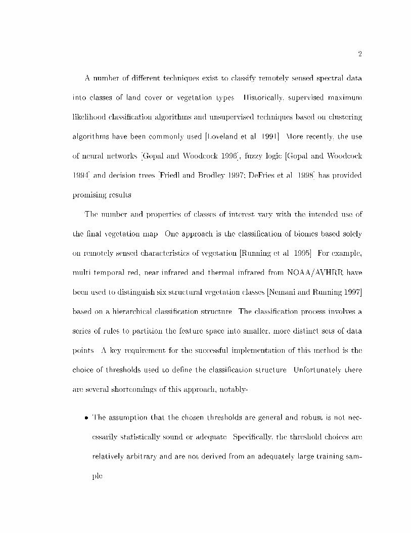
A number of di�erent techniques exist to classify remotely sensed spectral data

into classes of land cover or vegetation types. Historically, supervised maximum

likelihood classi�cation algorithms and unsupervised techniques based on clustering

algorithms have been commonly used [Loveland et al. 1991]. More recently, the use

of neural networks [Gopal and Woodcock 1996], fuzzy logic [Gopal and Woodcock

1994] and decision trees [Friedl and Brodley 1997; DeFries et al. 1998] has provided

promising results.

The number and properties of classes of interest vary with the intended use of

the �nal vegetation map. One approach is the classi�cation of biomes based solely

on remotely sensed characteristics of vegetation [Running et al. 1995]. For example,

multi-temporal red, near-infrared and thermal infrared from NOAA/AVHRR have

been used to distinguish six structural vegetation classes [Nemani and Running 1997]

based on a hierarchical classi�cation structure. The classi�cation process involves a

series of rules to partition the feature space into smaller, more distinct sets of data

points. A key requirement for the successful implementation of this method is the

choice of thresholds used to de�ne the classi�cation structure. Unfortunately there

are several shortcomings of this approach, notably-

� The assumption that the chosen thresholds are general and robust is not nec-

essarily statistically sound or adequate. Speci�cally, the threshold choices are

relatively arbitrary and are not derived from an adequately large training sam-

ple.

3

� The thresholds are speci�c to a particular data set.

� The method does not allow a reliable and systematic validation and assessment

of the classi�cation performance unless an independent validation dataset is

available.

One common approach to create a map in a desired classi�cation scheme is to

collapse an existing map with �ner class de�nitions into one with broader classes,

or alternatively to relabel class values according to a cross-walking rule set. This

approach has the following short-comings:

� The class de�nitions in the di�erent classi�cation schemes may not be compat-

ible, e.g., di�erent thresholds for the discrimination of vegetation density may

be used.

� It is often impossible to unambiguously cross-walk broad classes to a �ner res-

olution (e.g., forest to needleleaf forest and broadleaf forest).

� The cross-walking process can introduce confusion and errors which may then

be propagated through algorithms that use land cover as input.

The spectral information about the earth's surface to be measured by MODIS

and MISR will be the basis for a wide range of biophysical algorithms and products

(e.g., net primary productivity or leaf area index). For many of these algorithms land

cover is one of the most important input parameters. Therefore, inaccuracies in land

cover classi�cation will propagate through downstream algorithms.

4

The primary objective of this research is to generate a biome-based land cover

map for North America and compare its accuracy and properties with existing land

cover maps at the same scale and resolution. To this end, a decision tree classi-

�cation algorithm is used to create land cover maps in a 6-biome scheme and the

International Geosphere-Biosphere Program (IGBP) classi�cation scheme. The pri-

mary data source to train the classi�cation algorithm is a 12 month time series of

AVHRR NDVI in conjunction with ancillary data sources. Issues relating to cross-

walking between classi�cation schemes are addressed as well as methods to generate

a training sample for a supervised classi�cation of biomes.

This research speci�cally employs the biome based land cover classi�cation scheme

suggested by Myneni et al. [1997]. The underlying assumption of this classi�cation

scheme is that the earth's vegetation can be categorized in 6 structurally distinct

classes. Vegetation canopy structure is de�ned by plant geometry and distribution.

The classi�cation scheme is designed to complement an algorithm to retrieve global

leaf area index (LAI) and the fraction of absorbed photosynthetically active radiation

(FAPAR) from spectral re ectances from MODIS and MISR [Knyazikhin et al. 1998].

Speci�cally, radiative transer models (RTM) simulate the transport and interactions

of photons in vegetation canopies to retrieve information about plant structure from

re ected solar radiation. However, the parameterization of the RTM is dependent on

the structural characteristics of the plant canopy, which can be categorized in biomes.

The availability of high quality biome level maps of vegetation will be very useful to

this MODIS/MISR LAI/FAPAR retrieval algorithm.

5

2 Background

2.1 The Role of Land Cover in Biogeochemical Modeling

The importance of vegetation in global climate and biogeochemical cycles is well rec-

ognized [Sellers and Schimel 1993]. This is particularly true with respect to carbon,

which is �xed via primary production by terrestrial vegetation [Myneni et al. 1995].

The estimation of carbon �xation by terrestrial vegetation and the prescription of

accurate land surface properties requires variables descriptive of radiation absorp-

tion, plant physiology, climatology and surface assimilation area. As a consequence,

global biogeochemical models require accurate parameterization of the structural and

functional properties of plant canopies.

Hydro-meteorological conditions determine plant growth and structure in the

sense that plants adapt and grow by optimizing the use of resources like water, nu-

trients and solar radiation. These adaption processes can a�ect vegetation attributes

including plant size, leaf type, leaf longevity, density, and are fundamental mecha-

nisms for optimizing the energy absorption and dissipation under water availability

constraints [Woodward 1987].

Because of the diversity of global vegetation, there is an in�nite variety of plant

canopy shapes, sizes and attributes. In order to characterize plant canopies in a

useful way, leaf area index (LAI) and the fraction of absorbed photosynthetically

active radiation (FAPAR) have proven to be powerful parameters representing the

basic structural characteristics of vegetation canopies and their interaction with in-

6

coming solar radiation [Ruimy et al. 1994; Sellers et al. 1986]. LAI is de�ned as the

one-sided leaf area per unit ground area in broadleaf canopies and the projected or

total leaf area in needleleaf canopies and ignores the complexities of canopy geom-

etry. The characterization of vegetation by LAI, rather than species composition,

is a critical simpli�cation used to make global comparisons of terrestrial ecosystems

possible. LAI provides a measure of the physiology that is most directly involved in

energy, H2O and CO2 exchange processes. Strong correlation across di�erent vege-

tation types between LAI and net primary production (NPP), site water availability

and evapotranspiration (ET) have been found [Gholz 1982; Webb et al. 1983; Grier

and Running 1977; Jarvis and McNaughton 1986]. The fraction of absorbed photo-

synthetically active radiation by vegetation (FAPAR) exhibits diurnal variation and

therefore requires appropriate time integration for models with time steps longer than

one day [Myneni et al. 1997].

Remote sensing has established the relationship between LAI, FAPAR and spec-

tral vegetation indices, in particular the normalized di�erence vegetation index (NDVI)

(reviewed in Myneni et al. [1995]). The NDVI is de�ned as the ratio of the di�erence

in near-infrared and red re ectance normalized by their sum.

NDV I =NIR� RED

NIR +RED(1)

Asrar et al. [1992] found that under speci�c canopy conditions FAPAR was

linearly related to NDVI, whereas LAI exhibited a curvilinear relationship. Other

7

studies have shown that the relation between FAPAR and NDVI is similar for one-

dimensional and three-dimensional canopies [Myneni et al. 1992; Myneni andWilliams

1994]. The theoretical basis for the existence of those relations is described in Myneni

et al. [1995] and summarized in Myneni et al. [1997]. FAPAR is frequently used to

translate satellite data into simple estimates of primary production and photosyn-

thetic activity. However, it is important to note that di�erent biomes exhibit distinct

di�erences in their NDVI/LAI and NDVI/FAPAR relationships. Essentially, these

di�erences are used in the MODIS/MISR algorithm [Knyazikhin et al. 1998]. To

do this, a priori knowledge is required regarding the global distribution of biomes.

This thesis seeks to support the MODIS/MISR LAI/FAPAR algorithm by developing

improved methods to map biomes in an accurate and repeatable fashion at global

scales.

2.2 Global Land Cover Classi�cation Approaches

2.2.1 Conventional Approaches

Because of the diversity of vegetation at a global scale, the accurate mapping and

representation of terrestrial vegetation has been a challenge for many years. The

compilation of reliable databases at global scales involves both the generalization of

vegetation types into a smaller set of critical attributes and the development of means

for measuring vegetation globally in a meaningful timespan [Running et al. 1995].

Current global climate models, however, rely on land-cover data sets which are

8

typically derived from pre-existing maps and atlases [Olson andWatts 1982; Matthews

1983; Wilson and Henderson-Sellers 1985; Prentice et al. 1992]. This approach has a

number of limitations regarding model parameterization. First, the reference sources

themselves often represent a range of di�erent scales, dates and classi�cation schemes,

and the translation of mapping units into the classi�cation system and scale of in-

terest may introduce signi�cant new errors. Second, some datasets are derived from

maps of potential vegetation, which is usually inferred from climate variables rather

than the actual vegetation type. A third limitation is that many datasets are static

and are therefore prone to the perpetuation of errors in the source from which they

were derived [Loveland et al. 1991; DeFries et al. 1995].

A good illustration of the problems presented in this regard is given by Town-

shend et al. [1991], who compared existing maps of global vegetation and showed

that the estimates of vegetation distribution from common sources varied consider-

ably. The lack of consistency among the various map sources was attributed to both

the vegetation classi�cation and resolutions used in spatial sampling. While such

databases have obvious limitations, they represent the state of the science for driving

large scale process models.

2.2.2 Remote Sensing-Based Approaches

There is wide consensus that remotely sensed data can provide an accurate and re-

peatable means of land cover mapping and monitoring, especially with respect to

areas with rapidly changing landuse and land management activities [Running et al.

9

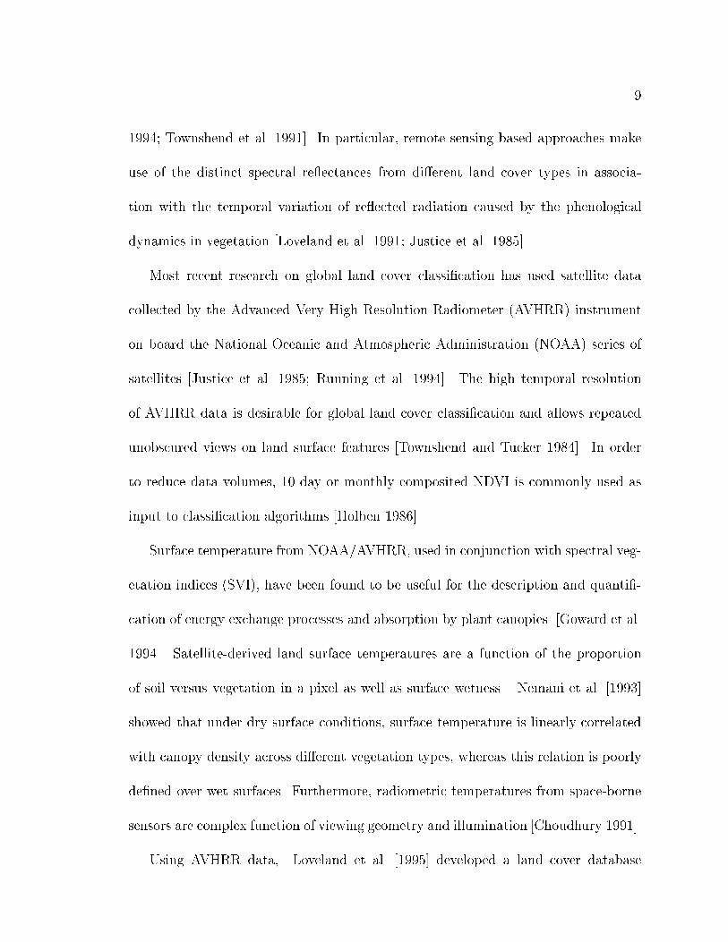
1994; Townshend et al. 1991]. In particular, remote sensing based approaches make

use of the distinct spectral re ectances from di�erent land cover types in associa-

tion with the temporal variation of re ected radiation caused by the phenological

dynamics in vegetation [Loveland et al. 1991; Justice et al. 1985].

Most recent research on global land cover classi�cation has used satellite data

collected by the Advanced Very High Resolution Radiometer (AVHRR) instrument

on board the National Oceanic and Atmospheric Administration (NOAA) series of

satellites [Justice et al. 1985; Running et al. 1994]. The high temporal resolution

of AVHRR data is desirable for global land cover classi�cation and allows repeated

unobscured views on land surface features [Townshend and Tucker 1984]. In order

to reduce data volumes, 10-day or monthly composited NDVI is commonly used as

input to classi�cation algorithms [Holben 1986].

Surface temperature from NOAA/AVHRR, used in conjunction with spectral veg-

etation indices (SVI), have been found to be useful for the description and quanti�-

cation of energy exchange processes and absorption by plant canopies [Goward et al.

1994]. Satellite-derived land surface temperatures are a function of the proportion

of soil versus vegetation in a pixel as well as surface wetness. Nemani et al. [1993]

showed that under dry surface conditions, surface temperature is linearly correlated

with canopy density across di�erent vegetation types, whereas this relation is poorly

de�ned over wet surfaces. Furthermore, radiometric temperatures from space-borne

sensors are complex function of viewing geometry and illumination [Choudhury 1991].

Using AVHRR data, Loveland et al. [1995] developed a land cover database

10

using an unsupervised classi�cation algorithm in conjunction with extensive ancillary

data. The unsupervised classi�cation yielded spectrally similar clusters of vegetation.

Ancillary data was then used to label those clusters. The �nal classi�cation included

205 classes for North America, which may be collapsed into fewer and broader set

of classes in a straightforward manner. However, their algorithm involves signi�cant

amounts of ancillary data and requires substantial manual post processing.

Most current classi�cation schemes designed for application at continental to

global scales are based on the magnitude and temporal dynamic of spectral vege-

tation indices such as NDVI [Justice et al. 1985; Loveland et al. 1991; Loveland et al.

1995; DeFries and Townshend 1994]. More recently, Nemani and Running [1997]

have demonstrated the potential of a combination of both spectral vegetation indices

(SVI) and surface temperature observations. Their methodology is based on known

energy exchange processes rather than statistical associations of vegetation types and

spectral properties.

The use of additional information in the training process, such as thermal bands

or seasonal metrics has also been suggested by DeFries et al. [1998]. Friedl et al.

[1999], however, showed that the use of additional phenological metrics provided little

improvement in classi�cation accuracy relative to using an annual time series of NDVI

data. Also, the use of geographic location as an input feature yielded substantially

better accuracies than using only NDVI. However, this does not re ect the true

accuracies and can be explained by interaction between the decision tree algorithm

and the bias introduced by the geographic distribution of training data.

11

Although the approaches described above provide promising results, it must be

noted that AVHRR data is limited in several regards including a high level of at-

mospheric noise (especially in channel 2), lack of onboard calibration, and only �ve

spectral bands [Zhu and Yang 1996; Cihlar et al. 1997; Moody and Strahler 1994]. As

a consequence, AVHRR data is insu�cient to discriminate subtle di�erences among

many vegetation types. The MODIS instrument is expected to overcome these limita-

tions for global land cover classi�cation. Speci�cally, it will provide superior spectral

and spatial resolution as well as better facilities for atmospheric correction and instru-

ment calibration. The speci�c properties of the MODIS instrument are documented

in Running et al. [1994] and Barnes et al. [1998].

Band AVHRR MODIS

Blue NA 0.459-0.479

Green NA 0.545-0.565

Red 0.580-0.680 0.620-0.670

NIR 0.720-1.10 0.841-0.876

SWIR NA 1.23-1.25

SWIR NA 1.63-1.65

SWIR NA 2.11-2.16

Table 1: Visible, red, near-infrared (NIR) and shortwave infrared bands (SWIR) for

AVHRR and MODIS

2.2.3 Biome-Based Classi�cation

As described above, climate and biogeochemical models require accurate input and

data on land cover [DeFries et al. 1995]. For example, Running and Hunt [1993]

introduced an ecosystem model (BIOME-BGC) designed to capture the essential

12

physio-morphological factors that regulate energy exchange processes in vegetation.

Within Biome-BGC, global vegetation is represented by six di�erent biome classes.

The ecological foundation for this classi�cation approach was given in Running et al.

[1995] and the classi�cation is based on three primary attributes of plant canopy

structure: (i) permanence of above ground biomass, (ii) leaf longevity and (iii) leaf

type or shape.

The �rst attribute, aboveground biomass, discriminates between permanent respir-

ing biomass, such as forests and woody shrubs, and annual crops and grasses. It is an

important determinant of carbon cycles and is controlled primarily by climate. Leaf

longevity, on the other hand, separates evergreen from deciduous canopies and plays

a major role in carbon and energy exchange processes. Finally, the leaf type criteria

distinguishes broadleaf and needleleaf plants as well as grasses. It also determines

the radiation and gas exchange characteristics of canopies.

The combination of these three criteria yields the following six biome classes: (1)

evergreen needleleaf, (2) evergreen broadleaf, (3) deciduous needleleaf, (4) deciduous

broadleaf, (5) broadleaf annual and (6) grasses. This classi�cation scheme has three

advantages over earlier classi�cation e�orts. First, it uses only plant attributes,

therefore other variables, such as climate, are excluded from the class de�nition.

Second, it is tailored to the information content of remotely sensed observations. Most

importantly, it provides a relatively stable and unambiguous classi�cation scheme for

the purpose of global biogeochemical modeling [Nemani and Running 1997].

Nemani and Running [1997] implemented this logic using a hierarchical classi�ca-

13

tion structure based on di�erent thresholds for NDVI, surface temperature and their

seasonality. However, the choice of thresholds is somewhat arbitrary and estimation

of the accuracy and performance of this algorithm can only be done using pre-existing

land cover maps. A somewhat similar biome classi�cation scheme based on canopy

architecture will be described in the next section in the context of radiative transfer

modeling of vegetation canopies.

2.3 Radiative Transfer Modeling of Vegetation Canopies

Canopy radiative transfer models (RTM) simulate radiation absorption and scatter-

ing in vegetation canopies. A review of canopy radiative transfer models can be found

in Myneni et al. [1995]. Myneni et al. [1997] suggested an algorithm for the esti-

mation of LAI and FAPAR at a global scale using such models. For a more detailed

description of three-dimensional radiative transfer modeling e�orts refer to Myneni

et al. [1990]. A synergistic algorithm for the estimation of vegetation canopy LAI

and FAPAR from MODIS and MISR data is described in Knyazikhin et al. [1998].

The relationship between NDVI and LAI/FAPAR has been established theoret-

ically. However, the utility of this relationship depends on the sensitivity of these

variables to canopy characteristics [Myneni et al. 1997]. While FAPAR exhibits a pos-

itive linear relationship with increasing NDVI, LAI is curvi-linearly related and shows

saturation with increasing NDVI (Figure 1). In order to estimate LAI/FAPAR from

remotely sensed data, canopy structural types must be de�ned that exhibit di�erent

14

0 2 4 6 8LAI

0.0

0.2

0.4

0.6

0.8

1.0

ND

VI

Broadleaf ForestsBroadleaf ForestsBroadleaf ForestsBroadleaf ForestsBroadleaf ForestsNeedle ForestsNeedle ForestsNeedle ForestsNeedle ForestsNeedle Forests

0.0 0.2 0.4 0.6 0.8 1.0NDVI

0.0

0.2

0.4

0.6

0.8

1.0

FPA

R

Broadleaf ForestsBroadleaf ForestsBroadleaf ForestsBroadleaf ForestsBroadleaf ForestsNeedle ForestsNeedle ForestsNeedle ForestsNeedle ForestsNeedle Forests

Figure 1: Relationships of NDVI/LAI and NDVI/FAPAR: Results for broadleaf

forests and needleleaf forests from prototyping e�orts with POLDER data (Zhang

et al., BU MODIS/MISR LAI/FAPAR team at Boston University).

NDVI-LAI or FAPAR relations from one another. If the canopy types have similar

NDVI-LAI/FAPAR relations, information on land cover is redundant for the esti-

mation of LAI/FAPAR. Therefore many classi�cation schemes, which are based on

ecological, botanical or functional metrics are not necessarily suitable for LAI/FAPAR

estimation.

The planned algorithm for the retrieval of LAI and FAPAR from MODIS/MISR

data is based on six distinct plant structural types (biomes), which can be parame-

terized with variables that many radiative transfer models employ [Knyazikhin et al.

1998].

This implies that a land cover classi�cation scheme that is compatible with radia-

tive transfer and LAI/FAPAR algorithms is needed. Myneni et al. [1997] de�ne the

following six biomes based on their canopy structure, which invoke di�erent radiative

transfer models to estimate LAI/FAPAR from remote sensing data.

15

Grasses and Cereal Crops (Biome 1): This land cover type is characterized by

vertical and lateral homogeneity, full ground cover and plant height less than about

a meter. The plants have erect leaf inclination, no woody material, minimal leaf

clumping and intermediate soil brightness.

Shrubs (Biome 2): Unlike biome 1, canopies are laterally heterogeneous and show

sparse to intermediate vegetation ground cover (20-60 percent). The plants have small

leaves, woody material, and bright backgrounds. This land cover type is typically

found in semi-arid regions with extreme temperature regimes and poor soils.

Broadleaf Crops (Biome 3): These canopies are laterally heterogeneous and ex-

hibit large variations in vegetation ground cover, ranging from about 10 percent after

planting to 100 percent at full maturity. They are characterized by regular leaf spa-

tial dispersion, a high level of photosynthetic activity in both leaves and stems, and

dark background soil.

Savannas (Biome 4): Savanna canopies have two distinct vertical layers, an un-

derstory of grass (biome 1) and an overstory of trees with about 20 percent ground

cover. Savannas in the tropical and sub-tropical regions are described as mixtures of

broadleaf trees and warm grasses, whereas in the cooler regimes of higher latitudes,

they are characterized as mixtures of cool grasses and needleleaf trees.

Broadleaf Forests (Biome 5): Broadleaf forests are characterized by both vertical

and horizontal heterogeneity, i.e. high ground cover, green understory, mutual crown

shadowing and foliage clumping. Trunks and branches are included in the radiative

transfer models, which means that canopy structure and optical properties di�er

16

spatially. Trunks are modeled as erect structures and branches as randomly oriented.

Needleleaf Forests (Biome 6): Needleleaf forests represent the most complex

canopy structure. They are characterized by needle clumping on shoots, shoot clump-

ing in whorls, dark vertical trunks, sparse green understory and mutual crown shad-

owing. Branches are modeled as randomly oriented and trunks as erect structures.

Needles are assumed to be clumped in the shoots, and the shoots clumped in the

crown space.

The de�nitions and properties of the six biomes as they relate to radiative transfer

are shown in table 2.

Grasses/

Cereal

Crops

Shrubs Broadleaf

Crops

Savannas Broadleaf

Forests

Needleleaf

Forests

Horizontal

Heterogene-

ity (Ground

Cover)

No

gc=100%

Yes

gc = 10-

60%

Variable

gc = 10-

100%

Yes

gc < 20%

Yes

gc > 70%

Yes

gc > 70%

Vertical

Heterogeneity

No No No Yes Yes Yes

Stems/

Trunks

No No Green

Stems

Yes Yes Yes

Understory No No No Grasses Yes Yes

Foliage

Dispersion

Minimal

Clumping

Random Regular Minimal

Clumping

Clumped Severe

Clumping

Crown

Shadowing

No NotMutual No No Yes Mutual Yes Mutual

Background

Brightness

Medium Bright Dark Medium Dark Dark

Table 2: Canopy structural attributes of global land covers from the viewpoint of

radiative transfer modeling [Myneni et al. 1997].

17

2.4 Tree-Based Classi�cation Algorithms

A suite of techniques are currently used to classify remotely sensed data into classes of

land cover. Traditionally, the vast majority of land cover mapping approaches have

used parametric supervised classi�cation algorithms or unsupervised classi�cation

algorithms. The latter use clustering techniques to identify spectrally distinct groups

of data [Schoewengerdt 1997]. These techniques have generally been used for high

resolution imagery, such as Landsat or SPOT.

Global land cover classi�cation e�orts, however, have mostly employed coarse

resolution data from NOAA/AVHRR [DeFries and Townshend 1994]. The literature

provides various examples of global land cover classi�cation e�orts. The more tradi-

tional approaches include unsupervised clustering in conjunction with ancillary data

and manual labeling of clusters [Loveland et al. 1991], maximum likelihood classi�ca-

tion [DeFries and Townshend 1994], and simple classi�cation logic based on structural

and biophysical parameters [Running et al. 1995].

More recent approaches include applications of neural networks [Gopal and Wood-

cock 1996], including fuzzy neural networks [Carpenter et al. 1992]. Neural networks

can handle relatively complex relations among the class properties, whereas tradi-

tional classi�cation algorithms are somewhat limited in their statistical and theo-

retical sophistication. However, neural nets need an understanding of theory and a

parallel processor to run real-time. They may not be a viable solution to all applica-

tions.

18

More recently, decision tree algorithms have been used for the classi�cation of

global datasets with promising results [Friedl and Brodley 1997; Friedl et al. 1999;

DeFries et al. 1998; Hansen et al. 1999]. Decision tree techniques have been used

successfully for a wide spectrum of classi�cation problems in various �elds [Safavian

and Landgrebe 1991]. They are computationally e�cient and exible, and also have

an intuitive simplicity. They therefore have substantial advantages in remote sensing

applications [Friedl and Brodley 1997].

A decision tree is a classi�cation algorithm which recursively partitions the feature

space of the data set into increasingly homogeneous subsets based on a set of splitting

rules. The tree has a root, which represents the entire data set, a set of internal nodes

(splits), and a set of terminal nodes (leaves). The nodes represent subsets of the data

set, while the terminal nodes at the bottom of the tree represent the predictions of

the tree. Every node in the tree (except the terminal nodes) has one parent node and

two or more descendant nodes. Each observation is labeled according to the majority

class of the leaf in which it falls [Breiman et al. 1984].

Running et al. [1995] and Nemani and Running [1997] applied a tree-based

decision structure to a global data set of NDVI values. The data set is both well

understood and well behaved and the classi�cation tree was de�ned solely on analyst

expertise, where the threshold values are de�ned based on ecological knowledge. This

algorithm, however, is somewhat di�cult to implement since signi�cant spatial, tem-

poral and spectral variation make globally robust user de�ned threshold speci�cation

almost impossible.

19

Figure 2: Decision tree structure

More commonly, tree-based algorithms use statistical procedures, which estimate

the classi�cation rules from a training sample. A classic example is the classi�ca-

tion and regression tree (CART) model described by [Breiman et al. 1984]. These

algorithms combine the advantages of statistically based techniques and learning al-

gorithms, which have their origin in the machine-learning and pattern-recognition

communities. Tree-based methods are supervised techniques and therefore a training

set is required from which the classes can be learned.

A critical step in the estimation of a decision tree is to prune the tree back in

20

order to avoid over�tting. By convention a tree is constructed in such a way that all

(or nearly all) training samples are correctly classi�ed, i.e. the training classi�cation

accuracy is 100%. If the training data contains errors the tree will be over�tted

and will generate poor results when applied to unseen data. Common methods for

pruning decision trees are described in [Mingers 1989] and brie y discussed in the

next section.

21

3 Methodology

The analysis for this thesis involved three main methodological components, each of

which is described in the sections below. Section 3.1 describes in detail the algorithm

that was used to generate land cover maps using both the IGBP and the 6-biome

classi�cation schemes. Section 3.2 explains the steps that were taken to translate

(cross-walk) the IGBP classes into biomes throughout the analysis. Section 3.3 dis-

cusses how the maps of UMD, EDC and BU were compared. Section 3.4 describes

the methodology used for map accuracy assessment.

3.1 Land Cover Classi�cation Algorithms

This section speci�cally focuses on the data used for the analysis, the major data

processing steps, the methods used for classi�cation performance evaluation, and the

decision tree parameters used for the classi�cation algorithm. Also, steps that were

undertaken to improve shortcomings in the training data are described.

The land cover classi�cation algorithm pursued in this research is based on the

concept of combining remotely sensed re ected and emitted radiation through time

and over space with ancillary data and information collected on the ground. The

underlying assumption is that the spectral information measured by satellites con-

tains information about plant canopy properties. NDVI is assumed to be a powerful

metric to represent these properties. The validity of this assumption is supported by

numerous studies in the past two decades [Tucker et al. 1986; Townshend et al. 1991].

22

The algorithm's goal is to distinguish land cover types on the basis of the spectral

and spatial properties of features on the Earth's land surface and their temporal

trajectories.

3.1.1 Data

The most commonly used source of satellite imagery for continental to global scale

studies is provided by the Advanced Very High Resolution Radiometer (AVHRR)

on board the NOAA series of satellites. The major advantage of AVHRR data over

other sources of satellite imagery is its high temporal resolution and global coverage.

Further, it provides su�ciently high spatial resolution (1.1km at nadir) for global

studies. However, its spectral properties are substantially less useful for land cover

classi�cation problems than Landsat Thematic Mapper (TM) data, for instance.

The classi�cation analyses presented below were based on a 12 month NDVI time

series. The data set is composed of monthly composited NDVI data covering the

time span between February 1995 and January 1996. In addition, seasonal land

cover regions (SLCR) labels [Loveland et al. 1991; Loveland et al. 1995] were also

tested as a predictive variable.

For supervised classi�cation approaches, a training sample is required to train the

classi�cation algorithm. To this end, a database of global land cover training sites has

been compiled and is currently being improved and extended by the MODIS Land

Cover and Land-Cover Change group at BU [Strahler et al. 1996]. The database

currently contains approximately 1000 sites distributed over the North American

23

continent (including sites in Central America) and has undergone several iterations

of reevaluation. Each site polygon in the database has an areal extent ranging be-

tween 2 and 100 km2 and a label assignment de�ned by the IGBP classi�cation

scheme (Loveland and Belward, 1997). Where possible, a set of biophysical parame-

ters has been assigned by the analyst to each training site. The label and attribute

assignments were performed using recent TM imagery from the multiresolution land

resource characterization database [Loveland and Shaw 1996] along with ancillary

data sources such as existing paper or digital maps, literature sources, aerial imagery

as well as veri�ed ground information from collaborating science teams. The suite of

site attributes is described in Muchoney et al. (1998).

3.1.2 Site Data Extraction and Classi�cation Estimation

The biome based classi�cation and map production essentially follows the algorithmic

steps developed by the MODIS Land Cover and Land-Cover Change group at Boston

University [Strahler et al. 1996]. These steps are:

1. Extraction of AVHRR NDVI pixel values for each training site and assignment

of class labels from training site database.

2. Manual detection and removal of multivariate outliers in the training data.

3. Tree estimation and pruning.

4. Cross-validation evaluation of classi�cation performance using independent train

and test datasets.

24

5. Analysis of classi�cation performance.

To extract the respective NDVI values for each training and test site from the

AVHRR imagery, careful and accurate registration of each site to geographic coordi-

nates needs to be assured. To this end, each training site polygon was registered to

coordinates in the Universal Transverse Mercator Projection (UTM), converted to a

raster image format with a 30m resolution, aggregated to a 1km resolution and repro-

jected to the Integerized Sinosoidal Grid (ISG) Projection used for MODIS products.

In this projection the globe is tiled into a grid of 25x17 cells, of which 326 contain

land mass. Each tile has an extent of approximately 1200x1200 km 1 .

A key step in the training database development is to remove statistical outliers

in order to avoid unwanted confusion in the classi�cation algorithm. To do this, a

two step generalized gap test for multivariate outlier detection was performed [Rohlf

1975]. In the �rst step, the largest pixel outliers in each training site were removed

from the training data with the intent of increasing the homogeneity in each site. In

the second step, sites were identi�ed as outliers within each class to decrease within-

class heterogeneity. Examples of an outliers in shown in Figure 4. A total of 35 sites

(768 pixels) were removed from the training data based on this analysis.

Classi�cation performance was assessed using cross-validation procedures. Specif-

ically, the population of the training data was randomly split into 5 mutually exclusive

training samples consisting of 80 percent of the data and an independent test sample

1For a detailed description of the Hierarchical Data Format (HDF) used by the Earth ObservingSystem and MODIS data storage and gridding, the reader may refer to http://daac.gsfc.nasa.gov/and [Wolfe et al. 1998]

25

Figure 3: Data processing ow

consisting of the remaining 20 percent. For each 80/20 split a decision tree was esti-

mated using the training sample and its performance evaluated on the independent

test sample. In this way, the information contained in the test sample was previously

unseen (independent) and not used to build the tree. The classi�cation accuracies

herein are reported as averages across the �ve cross-validation runs.

Since the training sites were de�ned in a way such that the within-site homogeneity

is maximized, substantial spatial autocorrelation was present in the AVHRR data

26

Month

ND

VI

2 4 6 8 10 12

100

120

140

160

180

200

NDVI Trajectory for Max Outlier Class: 2 #Sites = 38 Site ID = 340

Month

ND

VI

2 4 6 8 10 12

100

120

140

160

180

200

NDVI Trajectory for Max Outlier Class: 1 #Sites = 45 Site ID = 419

Month

ND

VI

2 4 6 8 10 12

100

120

140

160

180

200

NDVI Trajectory for Max Outlier Class: 14 #Sites = 61 Site ID = 424

Month

ND

VI

2 4 6 8 10 12

100

120

140

160

180

200

NDVI Trajectory for Max Outlier Class: 4 #Sites = 51 Site ID = 793

1

Figure 4: Examples of multivariate statistical outliers in the training database. The

solid line represents the trajectory of the mean maximum NDVI value for a class.

The diamonds show the monthly mean maximum NDVI values for the largest outlier

in a site.

within sites 2 . Spatial autocorrelation can have a signi�cant impact on accuracy

assessment measures [Congalton 1988] and in uence accuracy coe�cients. That is,

two features in space are likely to be autocorrelated, when they are close to each

other. Conceptually speaking, the prediction of a pixel's value becomes \easier" for

the classi�cation algorithm based on prior information about adjacent pixels [Friedl

2Spatial autocorrelation occurs when the presence, absence, or degree of a certain characteristica�ects the presence, absence, or degree of the same characteristic in neighbouring units [Cli� andOrd 1973]

27

et al. 1999]. Therefore, both pixel-based and site-based accuracies are reported here.

For pixel-based accuracies the training data was randomly split on a per-pixel level.

That is, pixels used to estimate the decision tree may be used to predict other pixels

from the same site. For site-based accuracies on the other hand, the splits were

constrained by the site membership, which means that pixels from 80% of the sites

were used to predict the remaining 20% of the sites, which are spatially separated.

The processing steps described above allow a statistically sound evaluation of the

classi�cation performance on a given data set. To produce the �nal map, all the

training data were pooled and a �nal tree was built based on the entire training data

set. This tree was then used to classify the NDVI image dataset.

3.1.3 Decision Tree Parameters

For this analysis C5.0, a widely used and tested univariate decision tree algorithm, was

used. A detailed description of the algorithm can be found in [Quinlan 1993]. The

most important elements, however will be discussed brie y here. The method used by

C5.0 to estimate the splits at each internal node of the tree is called the information

gain ratio. This metric measures the reduction in entropy in the data produced by

a split, and the split which maximizes the reduction in entropy in descendant nodes

is selected. The algorithm is terminated when no more gain is yielded by further

splitting [Quinlan 1993]. Unlike other trees used in global land cover classi�cations

(e.g. DeFries et al. 1998) the �nal tree is often very complex and large, and the tree

may be over�t to noise in the data. Errors in the training data can therefore lead

28

to poor performance on unseen (independent) cases. C5.0 addresses this problem by

using error-based pruning, i.e. the tree is \cut back" until all parts of the tree are

removed that have a high predicted error rate based on unseen cases [Mingers 1989;

Quinlan 1987]. For this analysis a conservative value of 5 percent pruning con�dence

was used.

A second important concept used in the C5.0 classi�cation algorithm is boosting,

a technique developed in the machine learning research community [Shapire 1990].

Boosting attempts to increase the classi�cation accuracy of a given learning algo-

rithm by iteratively estimating a number of classi�cations from the same data using

the same algorithm. At each iteration, weights are assigned to each training obser-

vation, where observations that were misclassi�ed in the previous iteration obtain a

higher weight than correctly classi�ed ones. This allows the algorithm to concen-

trate on cases that are more di�cult to classify. Friedl et al. [1999] demonstrated

that boosting can increase classi�cation accuracy in global land cover classi�cation

problems. When applied to di�erent datasets, boosting has been shown to increase

classi�cation accuracy with di�ering numbers of iterations. Based on the results

of Quinlan [1996] and Friedl et al. [1999], this research applied boosting with ten

iterations.

29

3.2 Cross-Walking from IGBP Classes to Biomes

Cross-walking between di�erent classi�cation schemes if interest can not necessarily

be done in an unambiguous fashion and may introduce unwanted errors and inaccu-

racies. A critical step for the work presented here was to translate the training data

from the International Geosphere-Biosphere Program (IGBP) classi�cation scheme

into the biome classi�cation scheme (section 2.3). In particular, direct translation of

the 17 IGBP classes into the six biome classes is not possible for the IGBP classes

5, 6, 8, 12, 14 (mixed forest, closed shrublands, woody savanna, croplands and crop-

lands mosaic, respectively; for detailed de�nition of the classes refer to Table 23 in

the appendix).

To resolve these ambiguities, the seasonal land cover region characterization (SLCR)

[Loveland et al. 1995] was used as an ancillary data source. This map possesses sig-

ni�cantly more classes than the IGBP scheme and therefore much narrower class

de�nitions. The SLCR project de�ned approximately 200 classes for each of the �ve

continents (205 classes for North America, 963 globally). The narrow de�nition of

the SLCR classes allows their aggregation into broader classes of other classi�cation

schemes, e.g., the IGBP scheme. Look up tables (LUT) for the aggregation of SLCR

classes into various existing classi�cation schemes are provided by EDC and used as a

guideline for the translation to 6 biomes performed for this work. For a more detailed

description of the SLCR map product and its classi�cation scheme the reader may

refer to Loveland et al. [1995].

30

IGBP Biomes

1 Evergreen Needleleaf Forests (ENF) Grasses and Cereal Crops (Biome 1)

2 Evergreen Broadleaf Forests (EBF) Shrubs (Biome 2)

3 Deciduous Needleleaf Forests (DNF) Broadleaf Crops (Biome 3)

4 Deciduous Broadleaf Forests (DBF) Savannas (Biome 4)

5 Mixed Forests (MXF) Broadleaf Forests (Biome 5)

6 Closed Shrubland (CSH) Needleleaf Forests (Biome 6)

7 Open Shrubland (OSH) Non-Vegetated (Biome 7)

8 Woody Savannas (WSA)

9 Savannas (SAV)

10 Grasslands (GRL)

11 Permanent Wetlands (PWL)

12 Croplands (CRL)

13 Urban and Built-up (URB)

14 Cropland Mosaics (CRM)

15 Snow and Ice (SNI)

16 Barren or Sparsely Vegetated (BSV)

17 Water Bodies (WAT)

Table 3: Comparison of the IGBP and biome classi�cation scheme [Loveland et al.

1995; Myneni et al. 1997]

For this work a LUT based on those provided by EDC were used to assign a biome

label to each training site for those cases where the training site possessed an ambigu-

ous IGBP label (classes 5, 6, 8, 12, 14, 16). The relabeled training sites were then

used as input to the classi�cation process as described above (pre-classi�cation ag-

gregation). To accomplish this task, a SLCR label for each training site was obtained

by overlaying training site polygons with the SLCR map. The most common class

within the training site polygon was used as a SLCR label. The SLCR and IGBP

labels were then compared and examined for agreement. In 40 cases the training site

label and the corresponding SLCR label were not in agreement and were therefore

31

removed from further analysis.

Note that the use of the SLCR labels introduces a bias to the EDC map, which is

based on the SLCR map. That is, the training site label assignment was not directly

done by an expert, but was based on an ancillary data source, which was evaluated

later using the same data. Unfortunately, no other independent map with narrow

class de�nitions is available at this point which could be used as an independent data

source for this purpose.

3.3 Comparison of UMD, EDC and BU Maps

In the second part of the analysis a quantitative comparison of land cover map prod-

ucts provided by the EROS Data Center (EDC) and University of Maryland College

Park (UMD) was performed. This served two purposes. First, it provided an ad-

ditional way to assess the properties of the maps produced with the decision tree

classi�cation algorithm. Second, it highlighted the strengths and weaknesses of each

map and helped to decide, which map to use for global retrieval of LAI and FAPAR

by the Vegetation and Climate Research Group (section 5.4). While the map pro-

duced by EDC was created using a classi�cation approach based on an unsupervised

algorithm with subsequent labeling of spectral classes, UMD uses an approach sim-

ilar to BU. For detailed description of the respective classi�cation algorithms, refer

to [Hansen et al. 1999] and [Loveland et al. 1995].

The classi�cation scheme used by UMD follows essentially the IGBP classi�cation

32

logic. However, three IGBP classes are not included in the UMD scheme: snow and ice

(IGBP 15), permanent wetland (IGBP 11) and cropland mosaic (IGBP 14). Therefore

these three classes were excluded from further analysis. Furthermore, the UMD class

names and class numbers do not always correspond to the IGBP class names, even

though the class de�nitions are the same. For the purpose of this analysis, the UMD

map was recoded to correspond to the IGBP class numbers (Table 4).

Class Original UMD class number Recoded UMD class numbers

Water 0 17

ENF 1 1

EBF 2 2

DNF 3 3

DBF 4 4

MXF 5 5

WSA 6 8

SAV 7 9

CSH 8 6

OSH 9 7

GRL 10 10

CRL 11 12

BSV 12 16

URB 14 13

Table 4: Recoded UMD classes

The impact of misregistration on accuracy assessment and image analysis has been

previously demonstrated [Townshend et al. 1992]. Therefore, in order to perform a

meaningful comparison of the UMD, EDC and BUmaps, it was necessary to coregister

them accurately. To do this, the data and maps were analyzed and processed in the

Interrupted Goode's Homolosine map projection, which is commonly used for global

scale studies, and allows one-to-one mapping at global scales. That is, each pixel of

33

a continental to global scale map can be related to a corresponding pixels in another

map using the same pixel coordinates. A global map in the Goode's projection is

composed of a mosaic of 12 tiles in the Mollweide and the Sinusoidal projections,

which meet approximately at 40 degrees latitude [Steinwand 1994]. Reprojection of

source maps into other projections was avoided since it would have introduced errors.

The three map products were compared both qualitatively and quantitatively.

First, the areal extents of each class in the respective classi�cation scheme were com-

pared. Next, to provide a more rigorous analysis of the EDC and UMD maps, the

training site data from BU was used as reference data (\ground truth") to generate

accuracy statistics. Finally, by overlaying the maps, areas of agreement and disagree-

ment were identi�ed.

3.4 Accuracy Assessment

Classi�cation accuracy is typically assessed using an error or confusion matrix. This

matrix documents errors of omission and errors of commission by cross-tabulating per-

pixel labels output by the classi�cation algorithm with labels obtained from ground

truth mapping [Congalton 1991]. Errors of omission are calculated as the sum of all

o�-diagonal values in a row divided by the row total. They indicate the proportion

of sites or pixels in a particular class of the reference data that were not classi�ed

correctly by the algorithm. Errors of commission are calculated as the sum of all o�-

diagonal values in a column divided by the column total. They indicate the proportion

34

of sites or pixels in the map that were misclassi�ed by the algorithm. The total error

is calculated as the sum of all o�-diagonal values divided by the total of samples in

the matrix. Overall accuracies as well as conditional (i.e., class-speci�c) accuracies

can be computed by dividing the correctly classi�ed samples by the column, row or

matrix total, respectively. For this analysis the reference data are presented in rows,

whereas the test samples are presented in columns.

Error Matrix

#R/C! 1 2 ... q xk+ PAi

1 x11 x12 ... x1q x1+ x11=x1+

2 x21 x22 ... x2q x2+ x22=x2+

: : : ... : : :

q xq1 xq2 ... xqq xq+ xqq=xq+

x+k x+1 x+2 ... x+q

PUj x11=x+1 x22=x+2 ... xqq=x+q

Table 5: Arrangement of reference and test data in confusion matrix. #R refers to

the reference data, C! to the classi�ed (test) data.

The accuracy parameters used for this analysis are described below. Upper case

(P ) is used to denote summary parameters and lower case (x) denotes individual cell

values. Row and column totals are referred to as xk+ and x+k, respectively. The

total number of classes is q and the total number of pixels in the matrix is p. Using

this notation we have:

1. The overall proportion of area correctly classi�ed:

Po =1

p

qXk=1

xkk (2)

35

2. The Kappa coe�cient [Cohen 1960]:

� =

pqX

k=1

xkk �qX

k=1

xk+x+k

p2 �qX

k=1

xk+x+k

(3)

where

Pc =1

q2

qXk=1

xk+x+k (4)

Therefore � can be rewritten as:

� =Po � Pc1� Pc

(5)

3. User's accuracy PUj and commission error EUj for cover type j:

PUj =xjjx+j

EUj = 1� PUj (6)

4. Producer's accuracy PAiand omission error EAi

for cover type i:

PAi=

xiixi+

EAi= 1� PAi

(7)

The kappa coe�cient was introduced by [Cohen 1960] and provides a more re-

alistic estimation than a simple percentage agreement value because it considers all

cells in the error matrix and provides a correction for the proportion of chance agree-

ment between reference and test data [Rosen�eld and Fitzpatrick-Lins 1986]. PUj

describes the probability that a pixel classi�ed as class j in the map is labeled as

36

class j in the reference data. PAidescribes the probability that a pixel labeled as

class i in the reference data is classi�ed as class i in the map.

Each parameter uses di�erent information contained in the confusion matrix and

therefore summarizes the matrix in di�erent ways. While Pc and � provide a single

summary measure for the entire matrix, PUj and PAisummarize columns and rows,

respectively. However, since each of them obscures important details of the error

matrix, the full matrix is also reported [Stehman 1997].

It is important to note that error matrices with di�erent row and column totals

and a di�erent distribution of cell values may have the same overall accuracy or �

[Stehman 1997]. In order measure whether two matrices are signi�cantly di�erent,

the Z statistic is employed. This statistic allows to rank maps based on accuracy

coe�cients. Following the notation of Ma and Redmond [1995], Z for overall accuracy

is used as:

Z(Po) =Po2 � Po1q�2o2 + �2o1

(8)

For �, Z is used as:

Z(�) =�2 � �1q�2�2 + �2�1

(9)

The database of training sites compiled by BU provides extensive ground truth

for North America and can therefore also be used as an independent data set in

order to evaluate the EDC and UMD map. To compare maps, the same method can

37

be applied, except that each pixel of each map is compared rather than individual

polygons.

3.5 Improving Training Data Quality

Before the �nal analysis was performed, shortcomings in the training were improved

based on preliminary results and exploratory data analysis. This was accomplished

in three steps.

First, missing values in the AVHRR NDVI data (data dropout) introduced addi-

tional confusion in the classi�cation algorithm. This was in particularly a problem in

northern latitudes. In order to account for this problem, a set of temporal smoothing

and interpolation routines were applied to the dataset.

Second, due to misregistration of some of the TM scenes used in the training site

generation, not all sites could be used in the analysis. Out of the approximately 1000

sites only 665 were used. This had the consequence that areas in the northern part of

the continent were undersampled. In order to compensate for undersampled regions a

total of 32 new training sites was generated, based on areas of agreement between the

UMD and EDC map. This approach stems from the assumption that the con�dence

about the correct assignment of a class label is high where two independently gener-

ated maps agree. The sites were chosen randomly across the undersampled regions

with su�cient distance between each other in order to account for e�ects of spatial

autocorrelation. This method was also employed by Friedl and Brodley [1997].

38

Third, some categories were oversampled and introduced a bias in the classi�cation

algorithm to more frequent classes. In order to compensate for oversampled classes

the training data were resampled to re ect the expected proportions of land cover

classes on the North American continent. To do this, the proportions of each class

in the UMD and EDC maps were used as a guideline. In cases where the number of

training pixels available in a class was below the threshold required to characterize

the properties of the class, all the pixels were kept. In cases where the class size was

too large, a random sample proportional to the estimated frequency of this class on

the ground was generated and used for further analysis.

39

4 Results

This section discusses results from the analysis described above. Section 4.1 presents

results from the map generation in the IGBP and 6-biome classi�cation scheme. Sec-

tion 4.2 compares the accuracy coe�cients of the two maps, and section 4.3 includes

the results from the comparison of the EDC, UMD and BU maps.

4.1 Classi�cation Performance

The training data that were input to the classi�cation algorithm was processed in �ve

distinct iterations. Each iteration attempted to improve the quality of the maps and

increase accuracy coe�cients. The same methods and routines were applied to the

training data in both the IGBP and biome classi�cation schemes. In this section, the

iterations are refered to as I, II, III, IV and V. Each iteration has a particular training

data set and map associated with it. For each of iterations I-V accuracy assessments

were performed and the associated accuracy coe�cients are reported herein. The

estimated Z statistics demonstrate statistically signi�cant di�erences in classi�cation

accuracy between iterations.

Training set I represents the raw training data, without any data manipulation.

Training set II was manually cleaned for multivariate statistical outliers. Training

set III contains SLCR labels as an additional feature. Training set IV represents

the extended set with additional training sites added to it (i.e., SLCR labels in-

cluded). Training set V is training set IV with resampled proportions of land cover

40

and biome classes, respectively. Note that the reported accuracies are averages across

�ve-fold cross-validations. The results and the subsequent discussion mostly focus on

site-based accuracies, since these values were considered to provide a more rigorous

assessment of the classi�cation performance. The main results for the classi�cation

in the IGBP scheme are summarized in this section (Tables 6, 7 and 8). The full

error matrices from which the summary statistics are derived can be found in the

appendix (Tables 24, 25, 26, 27 and 28). The results for the classi�cation in the

biome scheme are also fully reported below.

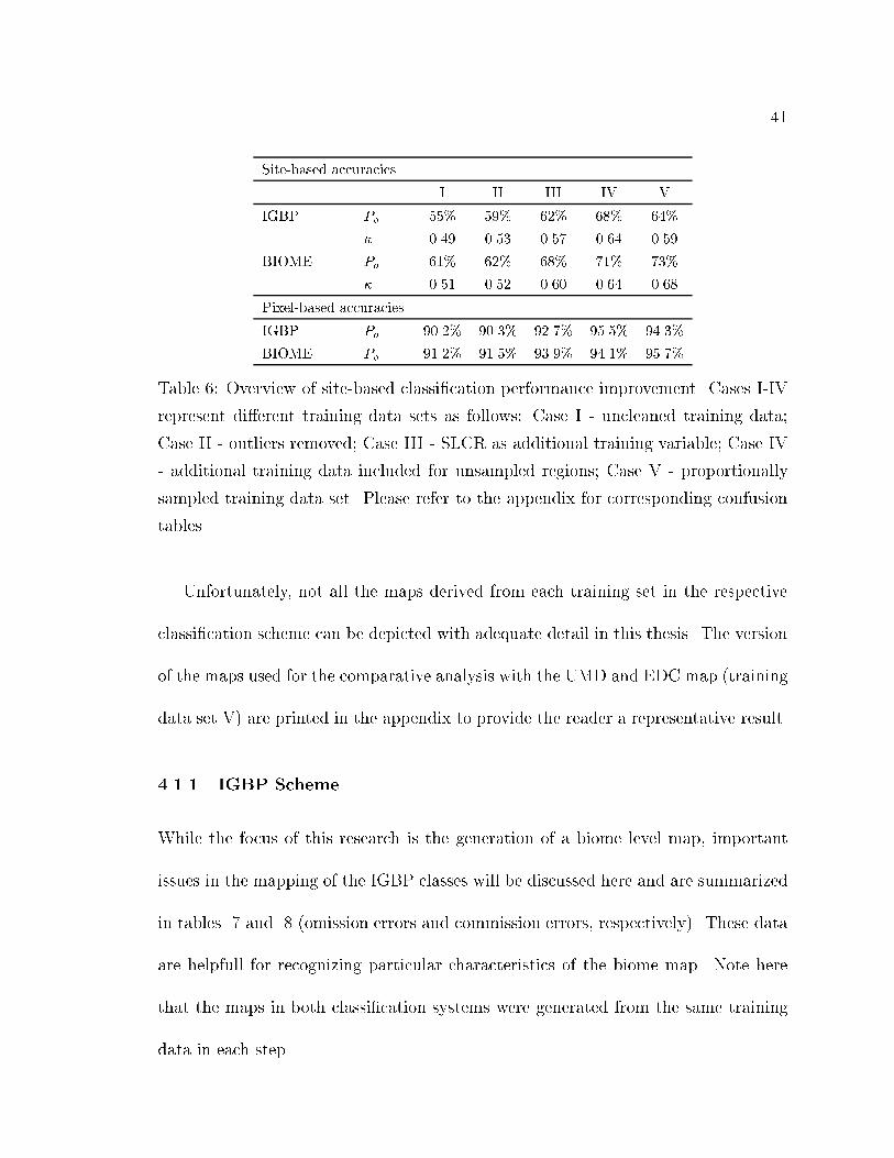
The results presented in table 6 show an increase in overall classi�cation accuracy

with each iteration. For the IGBP scheme, the overall accuracy was improved from

55% to 64%. The accuracies for the biome scheme are generally 5% higher and range

from 61% to 73%, respectively (Table 6). As expected, � is generally smaller than

Po since it accounts for chance agreement. However, the same trend is observed for

� with values ranging from 0.49 to 0.59 for IGBP classes and 0.51 to 0.68 for biome

classes.

Visual inspection of the class maps was a crucial step required to assess the

reliability of these results. Speci�cally each map was checked for overall patterns

and the distribution of land cover classes. This was particularly important since the

accuracy statistics do not necessarily re ect a meaningful or expected distribution of

land cover patterns. The results for two dominant land cover classes which control

much of the overall patterns of the maps, namely the forest and cropland classes, are

shown below and discussed in the next section.

41

Site-based accuracies

I II III IV V

IGBP Po 55% 59% 62% 68% 64%

� 0.49 0.53 0.57 0.64 0.59

BIOME Po 61% 62% 68% 71% 73%

� 0.51 0.52 0.60 0.64 0.68

Pixel-based accuracies

IGBP Po 90.2% 90.3% 92.7% 95.5% 94.3%

BIOME Po 91.2% 91.5% 93.9% 94.1% 95.7%

Table 6: Overview of site-based classi�cation performance improvement. Cases I-IV

represent di�erent training data sets as follows: Case I - uncleaned training data;

Case II - outliers removed; Case III - SLCR as additional training variable; Case IV

- additional training data included for unsampled regions; Case V - proportionally

sampled training data set. Please refer to the appendix for corresponding confusion

tables.

Unfortunately, not all the maps derived from each training set in the respective

classi�cation scheme can be depicted with adequate detail in this thesis. The version

of the maps used for the comparative analysis with the UMD and EDC map (training

data set V) are printed in the appendix to provide the reader a representative result.

4.1.1 IGBP Scheme

While the focus of this research is the generation of a biome level map, important

issues in the mapping of the IGBP classes will be discussed here and are summarized

in tables 7 and 8 (omission errors and commission errors, respectively). These data

are helpfull for recognizing particular characteristics of the biome map. Note here

that the maps in both classi�cation systems were generated from the same training

data in each step.

42

Needleleaf forests (IGBP class 1), deciduous broadleaf forests (IGBP class 4),

grasslands (IGBP class 10) and croplands (IGBP class 12) are the main land cover

classes on the North American continent and possess relatively distinct geographic

distributions. Independent source maps generally agree on the overall distribution

of these [Knapp 1965; Brown et al. 1998; Omernik 1987] classes. Therefore, visual

inspection concentrated on these classes. The results for these four IGBP classes are

shown below.

Needleleaf forests (class 1): Visual inspection of the maps produced by supervised

classi�cation revealed relatively poor results from the classi�cation algorithm for

training sample I. The error of omission for needleleaf forests was 59% (Table 7)

and a signi�cant portion of the pixels was incorrectly assigned to classes 12, 5, and 2

(croplands, mixed forest and broadleaf forests, respectively). Also, the same classes

contributed the majority of the total error of commission of 58% (Table 8). At the

same time, PAiincreased to 84% for steps I-V and the corresponding omission error

was reduced to 16% . The inclusion of additional training pixels for class 1 resulted

in a signi�cantly higher classi�cation performance and a better map with less obvious

confusions. Note that the contribution to the error of commission for class 1 by the

cropland classes were lowered from 10% to 1% (Tables 24 and 28 in the appendix).

Deciduous broadleaf forests (class 4): For deciduous broadleaf forests, omission

errors improved from 48% to 31% (Table 7) and commission errors from 48% to 28%

(Table 8) from steps I-V. In particular, the contribution to the error of omission by

class 12 was reduced from 7% to less than 0.5%. However, the added training sites

43

IGBP Total Omis- Contribution by individual classes

sion Error

Set I

ENF (1) 59% EBF(21%), MXF(16%), CRL(11%)

DBF (4) 48% MXF(13%), CRL(7%), CRM(8%)

GRL (10) 76% EBF(14%), CRL(23%), BSV(20%)

CRL (12) 37% GRL(5%), CRM(15%)

Set II

ENF (1) 48% EBF(12%), MXF(16%), CRL(9%)

DBF (4) 47% ENF(7%), MXF(10%), CRM(8%)

GRL (10) 68% EBF(13%), CRL(25%)

CRL (12) 28% ENF(4%), CRM(10%)

Set III

ENF (1) 39% MXF(15%), CRL(9%)

DBF (4) 44% MXF(16%), CRM(10%)

GRL (10) 71% EBF(15%), CRM(20%), BSV(14%)

CRL (12) 27% CRM(10%)

Set IV

ENF (1) 28% CRL(14%), MXF(6%)

DBF (4) 52% ENF(20%), GRL(5%)

GRL (10) 67% CRL(20%), BSV(14%)

CRL (12) 26% ENF(4%), CRM(9%)

Set V

ENF (1) 16% EBF(3%), MXF(6%)

DBF (4) 31% ENF(5%), EBF(7%), MXF(5%)

GRL (10) 47% OSH(10%), CRL(10%)

CRL (12) 53% GRL(10%), CRM(18%)

Table 7: Errors of omission for selected classes in the IGBP scheme.

introduced confusion with classes 1 and 2.

Note that these results do not distinguish the severity of the errors made. For

example, it can be argued that the confusion between croplands and forests is more

severe than confusion among forest classes. The relatively poor appearance of the

map based on training sample I is largely attributed to these types of commission

and omission errors.

44

IGBP Total Comis- Contribution by individual classes

sion Error

Set I

ENF (1) 58% EBF(10%), MXF(21%), CRL(10%)

DBF (4) 48% MXF(14%), CRM(13%)

GRL (10) 47% CRL(18%), BSV(14%)

CRL (12) 40% ENF(4%), GRL(9%), CRM(11%)

Set II

ENF (1) 52% DBF(5%), MXF(17%), CRL(9%)

DBF (4) 46% MXF(13%), CRM(10%)

GRL (10) 60% OSH(11%), CRL(10%) BSV(9%)

CRL (12) 39% GRL(9%), CRM(11%)

Set III

ENF (1) 43% EBF(6%), MXF(21%), CRL(6%)

DBF (4) 30% MXF(11%), CRM(5%)

GRL (10) 62% OSH(16%), CRL(12%), BSV(13%)

CRL (12) 36% GRL(8%), CRM(8%)

Set IV

ENF (1) 28% DBF(10%), CRL(4%), MXF(7%)

DBF (4) 29% MXF(8%), CRM(7%)

GRL (10) 52% DBF(9%), SAV(8%), BSV(9%)

CRL (12) 43% ENF(12%), GRL(7%), CRM(9%)

Set V

ENF (1) 18% MXF(9%)

DBF (4) 28% ENF(7%), MXF(8%)

GRL (10) 49% OSH(21%), BSV(10%)

CRL (12) 63% CSH(9%), GRL(16%), CRM(14%)

Table 8: Errors of commission for selected classes in the IGBP scheme.

In general, the confusion between both the needleleaf and broadleaf forest classes

with the mixed forest class was consistently high. This is not surprising since mixed

forest is a continuum of forest classes and is subject to analyst error. Further, spectral

information was not included in the classi�cation process and may have provided an

additional feature to resolve these misclassi�cations.

Grasslands (class 10): The grassland class exhibits signi�cant misclassi�cation

45

errors with respect to croplands and the sparsely vegetated/barren class. Also high

misclassi�cation rates were found with respect to broadleaf forests (14% for training

sample I, Table 7). Errors of both omission and commission with respect to classes

12, 14 and 16 improved. PAiimproved from 24% to 53%, and PUj from 33% to 51%

(Tables 24 and 28). The confusion with broadleaf forest was reduced in training

samples III and IV. The confusion of grassland with classes 12, 14 and 16 may be

explained as a function of their similar spectral signal, whereas the confusion with

broadleaf forest is probably due to a similar temporal signal.

Croplands (class 12): The distribution of croplands on the North American con-

tinent is very distinct due to ecological constraints and settlement structure and can

therefore be used to assess map properties in a qualitative way. Generally the mis-

classi�cation rates for other classes as croplands or cropland mosaic were very high

and was veri�ed by a quick visual assessment of each map. In particular, the occur-

rence of croplands in northern latitudes was a common weakness of all class maps and

could not entirely be solved. Oversampling of cropland in the initial training data is

assumed to be the major source of misclassi�cation. This assumption is supported

by visual inspection of the maps.

Decision tree algorithms are optimized to maximize classi�cation accuracy. As

a result, predictions are biased to more frequent classes. That is, the classi�cation

will tend to predict cropland for ambiguous cases, since this class is over-represented

in the training data. This observation was the motivation for applying proportional

sampling to the training data. The e�ect of proportional sampling is re ected in

46

PAiand PUj for class 12 (Tables 24- 28), where the initial accuracies were relatively

high, but dropped drastically for training sample V (63% to 47% and 60% to 37%,

respectively). Rescaling the proportion of cropland pixels in the training data had the

e�ect that confusion between class 12 and class 14 (cropland mosaic) became more

signi�cant and resulted in a drop. In the accuracies for these classes misclassi�cation

as grassland was also relatively high. This can be explained by the similarity of

NDVI trajectory between cereal croplands and grasses, which are most common in

the mid-western US. The over-representation of croplands in the training data base

can be likely attributed to the fact that they are easily discernible on TM images

and airphotos and are therefore frequently picked by analysts to designate a training

polygon.

4.1.2 Biome Scheme

The classi�cation performance for the biome classes was generally better than for

the IGBP classes (Table 6). Both producer's and user's accuracies improved for all

classes for steps I-V. Misclassi�cation of forest and cropland classes was found to be

the most signi�cant problem.

Grasses and Cereal Crops (Biome 1): Throughout the analysis, biome 1 exhibited

the highest errors of omission with respect to both needleleaf and broadleaf forests.

The contribution to the total omission error by broadleaf forest decreased from 14%

(Table 9) to 5% (Table 13). The magnitude of omission errors for classes 2, 3, 5 and

6 was generally only slightly lower. However, the degree of confusion is highest for the

47

Error matrix for uncleaned training data (I)

#R/C! 1 2 3 4 5 6 7 xk+ PAi

1 1213 212 193 163 350 192 189 2520 0.48

2 285 477 22 52 54 8 67 965 0.49

3 106 0 1286 81 107 134 9 1723 0.75

4 136 37 128 137 153 176 82 849 0.16

5 151 15 130 110 3745 330 69 4550 0.82

6 226 26 114 160 664 929 78 2197 0.42

7 188 31 12 90 23 51 602 998 0.60

x+k 2305 798 1885 793 5096 1820 1096 13793

PUj0.53 0.60 0.68 0.17 0.74 0.51 0.55

Trace = 8389 Po = 0.61 Pc = 0.20Pq

k=1 xk+x+k = 38759394 � = 0.51

Table 9: Error matrix for biome classes and site-based accuracy coe�cients for the

uncleaned training data set (I).

forest classes, which are structurally distinctly di�erent from biome 1. The misclassi-

�cation rate for biome 4 (savannas, e.g., in training set V, Table 13) of 6% compared

to 5% for broadleaf forests, very likely relates to the spectral properties of savannas,

which by de�nition possess up to 80% grass understory. Shrubs and needleleaf forest

exhibited the highest commission errors for biome 1. Shrubs contributed 14% to the

total commission error of 35% for training set V, needleleaf forests contributed 7%

(Table 13).

Shrubs (Biome 2): Shrubs showed the highest omission errors for biome 1 for

training set I-III. With the addition of supplemental training sites (V), misclassi-

�cation of shrubs as savannas increased drastically (33%, Table 12). This results

from the fact that the training samples previously did not contain samples of shrubs

from northern latitudes (tundra). Whereas the shrublands in the western part of

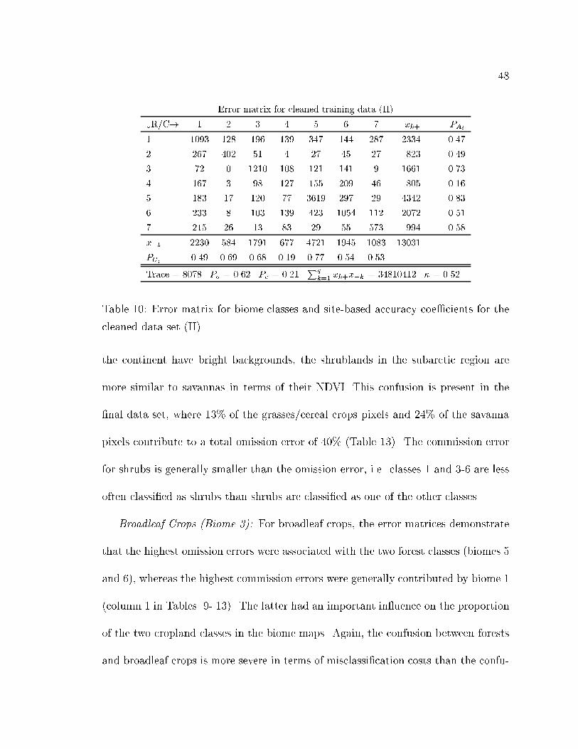
48

Error matrix for cleaned training data (II)

#R/C! 1 2 3 4 5 6 7 xk+ PAi

1 1093 128 196 139 347 144 287 2334 0.47

2 267 402 51 4 27 45 27 823 0.49

3 72 0 1210 108 121 141 9 1661 0.73

4 167 3 98 127 155 209 46 805 0.16

5 183 17 120 77 3619 297 29 4342 0.83

6 233 8 103 139 423 1054 112 2072 0.51

7 215 26 13 83 29 55 573 994 0.58

x+k 2230 584 1791 677 4721 1945 1083 13031

PUj0.49 0.69 0.68 0.19 0.77 0.54 0.53

Trace = 8078 Po = 0.62 Pc = 0.21Pq

k=1 xk+x+k = 34810412 � = 0.52

Table 10: Error matrix for biome classes and site-based accuracy coe�cients for the

cleaned data set (II).

the continent have bright backgrounds, the shrublands in the subarctic region are

more similar to savannas in terms of their NDVI. This confusion is present in the

�nal data set, where 13% of the grasses/cereal crops pixels and 24% of the savanna

pixels contribute to a total omission error of 40% (Table 13). The commission error

for shrubs is generally smaller than the omission error, i.e. classes 1 and 3-6 are less

often classi�ed as shrubs than shrubs are classi�ed as one of the other classes.

Broadleaf Crops (Biome 3): For broadleaf crops, the error matrices demonstrate

that the highest omission errors were associated with the two forest classes (biomes 5

and 6), whereas the highest commission errors were generally contributed by biome 1

(column 1 in Tables 9- 13). The latter had an important in uence on the proportion

of the two cropland classes in the biome maps. Again, the confusion between forests

and broadleaf crops is more severe in terms of misclassi�cation costs than the confu-

49

Error matrix for training data with SLCR as additional variable (III)

#R/C! c-> 1 2 3 4 5 6 7 xk+ PAi

1 1426 85 168 94 264 160 137 2334 0.61

2 318 346 36 7 18 16 82 823 0.42

3 152 1 1296 68 79 46 19 1661 0.78

4 183 0 95 180 144 150 53 805 0.22

5 188 5 98 49 3672 303 27 4342 0.85

6 207 24 71 89 330 1335 16 2072 0.64

7 171 21 17 61 71 16 637 994 0.64

x+k 2645 482 1781 548 4578 2026 971 13031

PUj0.54 0.72 0.73 0.33 0.80 0.66 0.66

Trace = 8892 Po = 0.68 Pc = 0.21Pq

k=1 xk+x+k = 35010219 � = 0.60

Table 11: Error matrix for biome classes and site-based accuracy coe�cients using

SLCR labels (III).

sion with biome 1. The best results were obtained for training sample V, where the

commission error for broadleaf and needleleaf forest was as low as 3% (Table 13).

Savannas (Biome 4): The accuracies for savannas improved from 16% to 52% for

PAiand from 17% to 32% for PUj (Tables 9 - 13, row 4 and column 4, respectively).

In the training sets I-III savanna pixels were largely misclassi�ed as one of the forest

classes or as grasses. This is clearly related to the properties of this class; speci�cally

the mixtures of both grasses and woodlands. Also, savannas represent a small portion

of the training data and were penalized by the classi�cation algorithm.

Broadleaf forests (Biome 5): Broadleaf forests had both the highest PAiand

PUj throughout the 5 iterations. The highest errors were observed with respect to

needleleaf forests and grasses/cereal crops. The latter is probably caused by a similar

temporal pattern of NDVI. The misclassi�cation of biome 5 as needleleaf forests can

50

Error matrix for training data with additional training sites (IV)

#R/C! 1 2 3 4 5 6 7 xk+ PAi

1 2107 130 223 74 231 259 128 3152 0.67

2 344 1736 39 1135 34 30 133 3451 0.50

3 70 3 1206 153 132 83 14 1661 0.73

4 143 5 117 510 128 179 105 1187 0.43

5 151 36 99 57 4706 278 37 5364 0.88

6 265 36 76 64 326 3148 36 3951 0.80

7 142 308 13 65 92 42 930 1592 0.58

x+k 3222 2254 1773 2058 5649 4019 1383 20358

PUj0.65 0.77 0.68 0.25 0.83 0.78 0.67

Trace = 14343 Po = 0.71 Pc = 0.17Pq

k=1 xk+x+k = 71726426 � = 0.64

Table 12: Error matrix for biome classes and site-based accuracy coe�cients with

additional training sites (IV).

be explained by naturally occuring mixtures of both classes.

Needleleaf forests (Biome 6): The major improvement in classi�cation perfor-

mance for needleleaf forests can be attributed to the addition of training sites, which

resolved the bias of broadleaf forest pixels in the previous training sets and the

undersampling of needleleaf forests in northern latitudes. The severest source of mis-

classi�cation are the classi�cation of needleleaf forests as grasses, which amounts to

11% in the uncleaned training sample (Table 9) and 6% in the last training sample

(Table 13). This problem could not be entirely resolved and is evident in the �nal

biome map (see Appendix).

The non-vegetated class showed an interesting interaction with the 6 biome classes.

In particular, biome 1 was frequently assigned to the non-vegetated class and vice

versa. This is not too surprising since many agricultural �elds are actually non-

51

Error matrix for training data with proportional sampling (V)

#R/C! 1 2 3 4 5 6 7 xk+ PAi

1 2089 197 122 188 151 256 85 3088 0.68

2 448 2091 27 839 24 34 36 3499 0.60

3 91 2 1240 126 90 91 7 1647 0.75

4 150 3 114 620 110 130 60 1187 0.52

5 53 16 42 63 2079 199 18 2470 0.84

6 241 21 45 68 220 3311 45 3951 0.84

7 153 45 16 64 21 45 1422 1766 0.81

x+k 3225 2375 1606 1968 2695 4066 1673 17608

PUj0.65 0.88 0.77 0.32 0.77 0.81 0.85

Trace = 12852 Po = 0.73 Pc = 0.16Pq

k=1 xk+x+k = 48961277 � = 0.68

Table 13: Error matrix for biome classes and site-based accuracy coe�cients for

proportional sampling (V).

vegetated for a number of months a year. Some misclassi�cation of class 7 as shrubs

was observed as well. Note that shrubs are de�ned by low vegetation density and

bright backgrounds, which is very similar to just bare ground. Supplementing addi-

tional training sites resolved these issues for the most part (Table 12).

The Z-statistic was used to test for signi�cant di�erences between the accuracy

coe�cients Po and � for the training sets I-V. These results are summarized in table

14. At a 5% con�dence level, error matrices are statistically signi�cantly di�erent if

Z > � 1.96 [Ma and Redmond 1995]. The table shows that each iteration's accuracy

coe�cients were signi�cantly di�erent from the previous iteration, respectively. For

the IGBP scheme the coe�cients for training set V were lower than for IV, which

resulted in a negative Z-score.

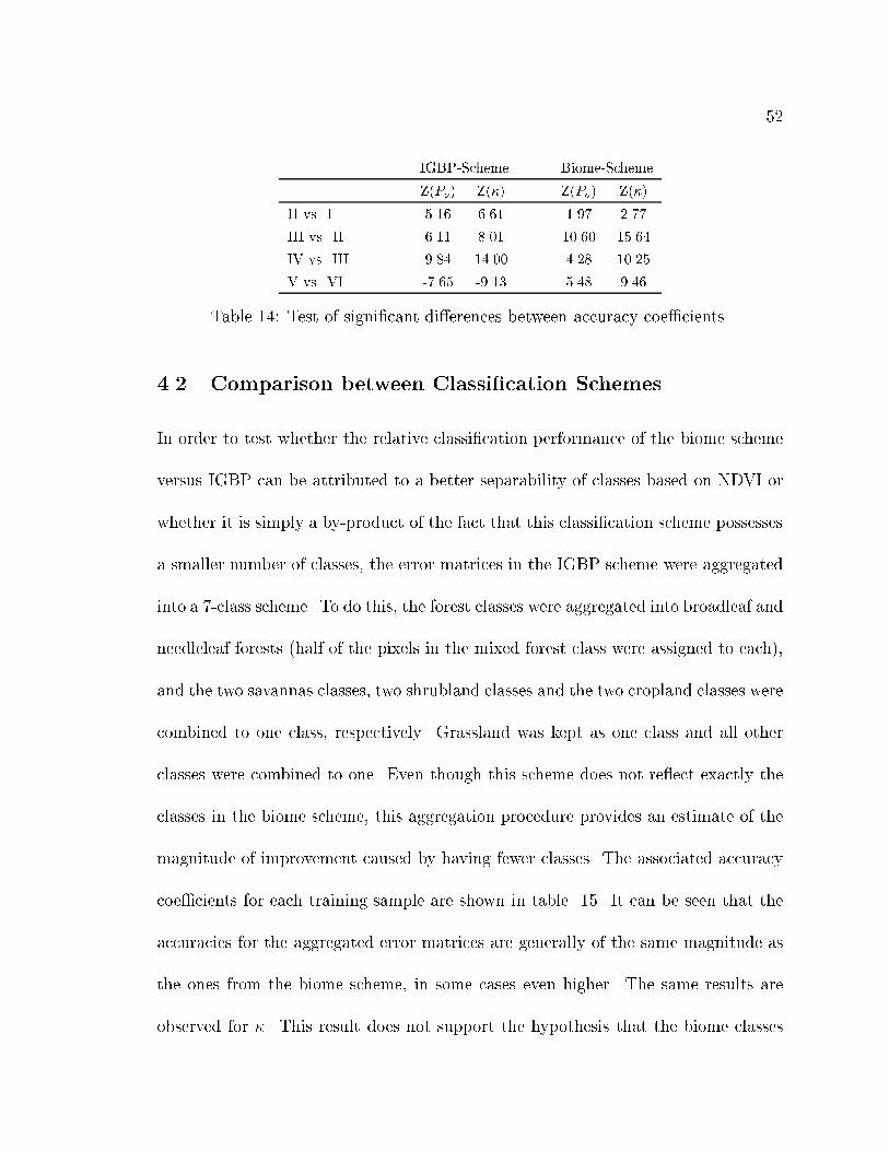
52

IGBP-Scheme Biome-Scheme

Z(Po) Z(�) Z(Po) Z(�)

II vs. I 5.16 6.61 1.97 2.77

III vs. II 6.11 8.01 10.60 15.64

IV vs. III 9.84 14.00 4.28 10.25

V vs. VI -7.65 -9.13 5.48 9.46

Table 14: Test of signi�cant di�erences between accuracy coe�cients.

4.2 Comparison between Classi�cation Schemes

In order to test whether the relative classi�cation performance of the biome scheme

versus IGBP can be attributed to a better separability of classes based on NDVI or

whether it is simply a by-product of the fact that this classi�cation scheme possesses

a smaller number of classes, the error matrices in the IGBP scheme were aggregated

into a 7-class scheme. To do this, the forest classes were aggregated into broadleaf and

needleleaf forests (half of the pixels in the mixed forest class were assigned to each),

and the two savannas classes, two shrubland classes and the two cropland classes were

combined to one class, respectively. Grassland was kept as one class and all other

classes were combined to one. Even though this scheme does not re ect exactly the

classes in the biome scheme, this aggregation procedure provides an estimate of the

magnitude of improvement caused by having fewer classes. The associated accuracy

coe�cients for each training sample are shown in table 15. It can be seen that the

accuracies for the aggregated error matrices are generally of the same magnitude as

the ones from the biome scheme, in some cases even higher. The same results are

observed for �. This result does not support the hypothesis that the biome classes

53

exhibit a stronger separability than the IGBP classes based on a time series of NDVI.

I II III IV V

Biome Scheme Po 61% 62% 68% 70% 73%

� 0.49 0.53 0.58 0.61 0.62

Aggregated IGBP classes Po 63% 66% 68% 73% 0.68%

� 0.52 0.56 0.58 0.67 0.62

Table 15: Accuracy coe�cients for aggregated IGBP maps into a 7-class scheme.

4.3 Map Comparisons

In this section, an accuracy assessment of the UMD and the EDC maps is presented,

using the training sites from the analysis above as reference data. The areal distri-

butions of land cover classes in the biome and IGBP are then compared with each

other. Error matrices are used to identify confusion among particular classes in both

classi�cation schemes. Maps of areal agreement are provided in the appendix.

4.3.1 Accuracy Coe�cients for the UMD and EDC Maps

In order to perform a site-based accuracy assessment for the UMD and EDCmaps, the

BU training sites were overlayed with each of the maps. However, not all of the sites

were used in the error matrices, because some sites were not entirely covered by one

class. The most frequent class of the respective map in each polygon was associated

with the site. For the IGBP scheme, only those sites were used in the comparison that

were covered with at least 75% of one class in both maps. For the biome scheme, those

sites that covered at least 90% of one biome. These thresholds were chosen because

54

they maximized the area covered by one class, while still maintaining a su�ciently

large sample in each category. Also, the sites that were detected as outliers in the

analysis above were not used in the error matrix. Unfortunately, this reduced the

number of available sites for the analysis.

Error matrix for UMD, 75% covered

#R/C! 1 2 4 5 6 7 8 9 10 12 16 xk+ PAi

1 24 0 2 13 0 0 3 0 0 0 0 42 0.57

2 0 26 2 0 0 0 2 0 0 0 0 30 0.87

4 4 1 13 30 1 2 5 1 1 1 1 60 0.22

5 2 0 6 16 0 0 2 0 0 0 0 26 0.62

6 0 0 1 1 0 1 2 0 1 0 0 6 0.00

7 0 0 0 0 1 1 0 0 1 0 0 3 0.33

8 0 3 0 0 0 3 0 1 2 0 0 9 0.00

9 0 0 0 1 0 0 1 0 0 0 0 2 0.00

10 0 0 0 0 1 2 1 1 6 3 0 14 0.43

12 0 0 1 4 0 0 0 3 2 11 0 21 0.52

16 2 0 0 0 0 1 2 0 2 0 1 8 0.13

x+k 32 30 25 65 3 10 18 6 15 15 2 221

PUj0.75 0.87 0.52 0.25 0.00 0.10 0.00 0.00 0.40 0.73 0.50

Trace = 98 Po = 0.44 Pc = 0.13Pq

k=1xk+x+k = 6197 � = 0.36

Table 16: Error matrix and site-based accuracy coe�cients for the UMD map in the

IGBP scheme.

It is important to note that the sites used for the analysis in the biome scheme

have a bias, since the SLCR labels were used to overcome ambiguities in cross-walking

the IGBP class labels to biome labels in the training site generation (section 3). Both

the EDC and UMD map were cross-walked using the SLCR-biome LUT.

EDC map: 254 sites were used for the accuracy assessment of the EDC map in

the IGBP scheme (Table 16). The overall accuracy was 47% and � was 0.38. Open

shrubland (class 7) and evergreen broadleaf forest (class 1) were found to have the

highest producer's accuracies (100% and 93%, respectively). Classes 5, 6, 8, 9, 11,

55

14 and 16 showed poor PAi(13% and less). In terms of user's accuracies most of the

classes performed relatively poorly, with exception of classes 1, 2, 3, 10, 12 and 16,

which showed at least 39% for PUj . Note that deciduous needleleaf forest (class 3) is

excluded in the table, since it was not classi�ed in either of the maps. Also, class 13

is not shown since an ancillary urban mask was used.

Table 19 shows the analysis for the EDC map in the biome scheme for 306 sites.

The overall accuracy was 84% and � was 0.76. Shrubs (biome 2) and broadleaf crops

(biome 3) had a PAiof 100%. Broadleaf forests were classi�ed with 96% accuracy,

whereas needleleaf forests showed only 59% for PAi. The table also shows high user

accuracies, in particular for biome 1, 3 and the non-vegetated category.

Error matrix for EDC using training data, 75% covered

#R/C! 1 2 4 5 6 7 8 9 10 12 14 16 xk+ PAi

1 26 0 13 4 0 0 0 0 0 0 0 0 43 0.60

2 1 28 1 0 0 0 0 0 0 0 0 0 30 0.93

4 4 1 39 6 1 2 3 1 1 1 1 1 61 0.64

5 3 0 19 3 0 0 1 0 0 0 0 0 26 0.12

6 1 0 3 0 0 1 0 0 1 0 0 0 6 0.00

7 0 0 0 0 0 3 0 0 0 0 0 0 3 1.00

8 0 3 0 0 0 3 1 0 1 0 1 0 9 0.11

9 0 0 1 0 0 0 0 0 0 0 1 0 2 0.00

10 0 0 0 0 0 3 1 3 6 0 1 0 14 0.43

12 0 1 5 0 0 0 0 0 1 13 1 0 21 0.62

14 0 0 6 0 0 1 0 0 5 18 1 0 31 0.03

16 3 0 0 0 0 3 0 0 0 0 1 1 8 0.13

x+k 38 33 87 13 1 16 6 4 15 32 7 2 254

PUj0.68 0.85 0.45 0.23 0.00 0.19 0.17 0.00 0.40 0.40 0.14 0.50

Trace = 121 Po = 0.47 Pc = 0.15Pq

k=1xk+x+k = 8883 � = 0.38

Table 17: Error matrix and site-based accuracy coe�cients for the EDC map in the

IGBP scheme.

UMD map: 221 sites were used for the accuracy assessment of the UMD map in

the IGBP scheme. Overall accuracy and � were 44% and 0.36, respectively. PAiwas

56

higher than 40% for classes 1, 2, 5, 10 an 12. User's accuracy was poor (25% and

less) for classes 5, 6, 7, 8 and 9. The other classes showed PUj greater than 40%.

Classes 3, 11 and 13 through 15 were not used (Table 16).

The results from the analysis of the UMD in the biome scheme are shown in table

19. Overall accuracy and � are 83% and 0.75, respectively. High PAiis shown for

biome 3 and 5. Biome 3 also shows the highest PUi of 100% as well as the non-

vegetated category.

Error matrix for UMD, 90% covered

#R/C! 1 2 3 4 5 6 7 xk+ PAi

1 24 3 0 5 0 2 0 34 0.71

2 2 5 0 0 0 0 0 7 0.71

3 0 0 18 0 0 0 0 18 1.00

4 0 0 0 5 1 0 0 6 0.83

5 0 1 0 1 143 5 0 150 0.95

6 0 0 0 1 27 39 0 67 0.00

7 1 0 0 1 1 0 19 22 0.86

x+k 27 9 18 13 172 46 19 304

PUj0.89 0.56 1.00 0.38 0.83 0.85 1.00

Trace = 253.00 Po = 0.83 Pc = 0.33Pq

k=1xk+x+k = 30683 � = 0.75

Table 18: Error matrix and site-based accuracy coe�cients for the UMD map in the

biome scheme.

4.3.2 Pixel-Based Comparisons

Tables 29- 31 and 32- 34 (Appendix) show pixel-based comparisons between these

two classmaps in the IGBP scheme and the biome scheme, respectively. The dif-

ferences between two class maps is represented best by a confusion matrix. This

representation shows the confusion of one class in map A with all other classes in

map B in one table. Note that in this case rows and columns do not refer to reference

57

Error matrix for EDC, 90% covered

#R/C! 1 2 3 4 5 6 7 xk+ PAi

1 24 3 0 5 0 2 0 34 0.71

2 0 7 0 0 0 0 0 7 1.00

3 0 0 18 0 0 0 0 18 1.00

4 0 0 0 5 1 0 0 6 0.83

5 0 1 0 0 144 5 0 150 0.96

6 0 0 0 1 27 40 0 68 0.59

7 1 1 0 1 1 0 19 23 0.83

x+k 25 12 18 12 173 47 19 306

PUj0.96 0.58 1.00 0.42 0.83 0.85 1.00

Trace = 257 Po = 0.84 Pc = 0.33Pq

k=1xk+x+k = 30913 � = 0.76

Table 19: Error matrix and site-based accuracy coe�cients for the EDC map in the

biome scheme.

and classi�ed data, but simply to di�erent maps in the same classi�cation scheme.

The diagonal values show the pixels that were classi�ed to the same class in both

maps. The sum of all diagonal values divided by the matrix total gives the overall

agreement of the two maps. PCiand PCj

refer to the proportion of pixels in agreement

in each row and column, respectively.

In tables 29 and 30 the UMD map is represented in rows and the BU and EDC

map in columns. Table 31 shows the BU map in rows and the EDC map in columns.

Note that the row and column totals do not exactly correspond to the histogram in

table 20. This is because classes that were excluded in the map comparison, e.g.

class 13 (urban and built-up) were masked in the analysis. The overall agreement

between the maps in all three classi�cation schemes is summarized in table 22.

The frequency of IGBP classes in the EDC, UMD and BU maps are shown in

table 20, the frequency of biome classes in table 21. The tables show that the areal

proportions in the three maps di�er signi�cantly. Note the high percentage of crop-

58

Frequency of IGBP classes in the EDC, UMD and BU maps

EDC UMD BU

Class Pixels % Pixels % Pixels %

1 3736947 17.0 2306360 10.5 3472296 15.9

2 354661 1.6 338431 1.5 356568 1.6

4 1488111 6.8 778641 3.6 1574119 7.2

5 2854132 13.0 1196545 5.5 948452 4.3

6 579582 2.6 1656401 7.6 398707 1.8

7 2306720 10.5 2970955 13.6 5047635 23.0

8 1571191 7.2 3263042 14.9 1469668 6.7

9 73694 0.3 3111528 14.2 316218 1.4

10 1658740 7.6 1977154 9.0 963878 4.4

11 359708 1.6

12 1852240 8.5 1818480 8.3 3693475 16.9

13 84539 0.4 84539 0.4 84539 0.4

14 1510139 6.9 1497631 6.8

15 1472376 6.7 1555290 7.1

16 1998884 9.2 2399588 11.0 605572 2.8

Total land mass = 21899509

Table 20: Frequency of classes in the IGBP scheme for the UMD, EDC and BU maps.

lands in the BU map. The distortion in proportion for the comparison in the biome

scheme are largely explained by the fact that these maps were generated using a

simple aggregation scheme (see maps in the Appendix). This demonstrates how sig-

ni�cant the errors may be if a map is aggregated to the biome scheme using simple

cross-walking rules.

59

Frequency of IGBP classes in the EDC, UMD and BU maps

EDC UMD BU

Class Pixels % Pixels % Pixels %

1 1658740 7.5 1647527 7.5 3686851 16.8

2 2306720 10.5 2947821 13.4 4896929 22.4

3 1852240 8.5 1429950 6.5 1378206 6.3

4 1644885 7.5 5627713 25.7 1847457 8.4

5 5276486 24.1 3632644 16.6 2006770 9.1

6 3736947 17.1 2262153 10.3 5337426 24.4

7 3555799 16.2 2484009 11.3 2748025 12.5

Total land mass = 21899509

Table 21: Frequency of classes in the biome scheme for the UMD, EDC and BU

maps.

IGBP Biome

UMD vs. EDC 38.8% 45.5%

UMD vs. BU 36.3% 42.7%

EDC vs. BU 38.3% 47.6%

Table 22: Overall agreement of the UMD, EDC and BU maps in the IGBP and biome

classi�cation scheme.

60

5 Discussion

The analysis involved four main components: training data improvement, classi�-

cation performance in the IGBP scheme, classi�cation performance in the biome

scheme, and map comparison. These four components will be discussed in the sub-

sequent section.

5.1 Training Data Improvement

The initial generation of maps in both classi�cation schemes provided important

insights into shortcomings of the training data. In particular, maps derived from the

extracted training data without any further pre-processing yielded poor results. The

associated site-based map accuracies were 55% for the IGBP scheme and 61% for the

biome scheme. Major types of misclassi�cation errors were observed for IGBP classes

12 and 14 (cropland and cropland mosaics) and biome classes 1 and 3 (grasses/cereal

crops and broadleaf crops). In higher latitudes, these classes were frequently confused

with needleleaf forests. These errors were attributed to four main factors.

First, mislabeled or noisy training sites were found to introduce errors in the

classi�cation algorithm. These problems were generally related to errors made in the

training site database generation. Some sites were too heterogeneous in their NDVI

signal, and others were likely to be mislabeled or incorrectly georeferenced. Also,

dropouts in the AVHRR data caused problems.

Second, seasonal trajectories of NDVI data were limited in their ability to predict

61

and discriminate certain classes from the given training data provided. For example,

the trajectories of certain cropland training sites were not distinct from grassland

sites.

Third, the representation of certain land cover classes in the training data was

insu�cient. In particular, regions in northern latitudes were undersampled, because a

number of training sites could not be used in the analysis due to misregistration errors.

This particularly a�ected predictions of tundra (shrublands) and boreal needleleaf

forest.

Fourth, cropland classes were oversampled in the training data and C5.0 tended

to overpredict these classes. This was mainly a problem in high latitudes, where

needleleaf forest were misclassi�ed as croplands.

These issues were addressed in four steps of training data improvement and are

re ected in the training sets I-V. Manual removal of within-site and within-class

outliers (step I) resulted in an improvement of 4% in overall accuracy for the IGBP

scheme, but only 1% for the biome scheme. Note that the outlier detection was

performed for IGBP classes, i.e., if a pixel or a site was identi�ed as a multivariate

outlier in the IGBP scheme, the same pixel or site was removed from the training

data in the biome scheme. In this context, the smaller improvement produced for the

biome classi�cation scheme was probably caused by the narrower de�nition of the

IGBP classes, i.e., an outlier that was identi�ed within an IGBP class, may not be

an outlier within biome classes. Even though this method involved a certain degree

of subjectivity, con�dence was high that mislabeled and extremely heterogeneous

62

sites were removed from the training data. Unfortunately, the improvement due to

temporal smoothing of the AVHRR data was not quanti�ed in this analysis. However,

signi�cantly less artifacts were detected upon visual inspection of the maps.

The baseline dataset (step I) was not adequate to classify major ecological re-

gions. Visual comparison of each of the maps produced with existing vegetation

maps [Omernik 1987; Bailey 1996; Knapp 1965; Brown et al. 1998] revealed weak-

nesses regarding the overall pattern and distribution of land cover types. The use

of SLCR labels improved the maps signi�cantly and the patterns were generally in

better agreement with other map sources and expert knowledge. Note that the SLCR

labels were produced using extensive ancillary data in a labor intensive fashion [Love-

land et al. 1995] and provided high quality input to the classi�cation algorithm. The

analysis of the decision tree created from the training data in association with SLCR

labels showed that the SLCR labels were frequently selected as a decision feature,

but did not outweigh NDVI. The percentage of SLCR labels chosen as a feature in

the decision tree ranged from 20-25%. This number can only be estimated from mul-

tiple trees that were generated by boosting. This indicates the magnitude of the bias

introduced by using the SLCR labels in the training process.

Unfortunately, a signi�cant portion of the training sites could not be used in the

analysis due to misregistration errors (approximately 400 out of 1000 sites). The gen-

eration of additional training sites using the EDC and UMD maps was therefore an

important step in improving the properties of the �nal maps. Undersampled regions

were mostly located in northern latitudes where land cover is generally homogeneous.

63

Even though no outlier detection was performed on these sites, con�dence was high

that these sites were of good quality, since the EDC and UMD were in agreement.

This observation is underscored by the improvement in overall accuracy from 62% to

68% for the IGBP map and 68% to 71% for the biome map in step IV. It is acknowl-

edged that the use the UMD and EDC to generate new training sites introduces an

additional source of uncertainty that can not be accounted for. Nonetheless, this step

was important to supplement the classi�cation algorithm with undersampled regions.

Proportional sampling of classes in step V was particularly important since the

frequency distribution of land cover types in the training data did not re ect the

proportions of land cover types in other maps. The overall accuracy of 68% for the

IGBP class in step IV is partly attributed to a bias towards overpredicting class

12 (which was oversampled in the training data). Once this bias was removed the

accuracy dropped 4% in step V. This e�ect was not observed for the biome classes,

because the training data were rescaled to account for the smallest class in the dataset.

Therefore, the bias in the IGBP results was more pronounced than in the biome data.

It must be noted that shortcomings in the sampling design will a�ect the accu-

racy statistics derived from the training data [Congalton 1991; Stehman 1996]. The

sample of training sites is biased in three ways with respect to the SLCR map. First,

the SLCR labels were used to cross-walk the IGBP labels in the training data to

biome labels. Second, the SLCR were also used as a feature in the estimation of the

tree. Third, the generation of training sites used the SLCR map as a guideline for

a strati�ed sampling scheme. Unfortunately, only few alternative map sources are

64

available at continental scales that could serve as sampling strata. For example, the

maps generated by Omernik [1987] and Bailey [1996] provide an alternative for an in-

dependent sampling stratum. The accuracies reported herein are therefore expected

to contain errors and do not necessarily represent the exact accuracies. However, it is

di�cult to quantify the magnitude of this bias. The issues relating to shortcomings

in the sampling scheme could not be addressed in this work and need to be assessed

in the future. But it also has to be kept in mind, that the generation of a statistically

sound training site sample at global scales is extremely expensive and labor intensive.

Visual inspection was a very important tool in the production of land cover maps

and allowed identi�cation of weaknesses in the training data. This is a very com-

mon approach in supervised classi�cation and is frequently reported in the literature

[DeFries et al. 1998].

The land cover maps from EDC and UMD are the only comparable land cover

map products at a global to continental scale derived from 1 km AVHRR data. Un-

fortunately, accuracy coe�cients associated with these maps are yet to be published.

Therefore, the accuracies reported herein can only be benchmarked against results

from classi�cation e�orts at a di�erent spatial resolution. Also, pixel-based accu-

racies are generally reported in the literature. This research, however, focused on

site-based accuracies.

DeFries et al. [1998], for example, reported pixel-based overall accuracies ranging

from 81.4% to 90.3% using di�erent phenological metrics for a global land cover

classi�cation using 8km AVHRR data. However, validation of these map products

65

was based on the same data that was used to train their supervised classi�cation

algorithm. Therefore, these accuracies are expected to be biased. Friedl et al. [1999]

assessed the impact of boosting, phenological metrics and geographic location in

an supervised classi�cation process using the 1 degree land cover set compiled by

DeFries and Townshend [1994] and the EDC IGBP land cover map for North America

[Loveland et al. 1995]. The associated accuracies ranged from 78.7 to 96.6% and from

67.4 to 79.5%, respectively. The 96.6% overall accuracy associated with the 1 degree

dataset, however, was mostly attributed to the e�ect of using geographic location in

the classi�cation process and was not considered to be representative for the true

accuracy of the dataset. Also, non-independent splits of train and test data are

expected to cause a bias in the accuracy assessment.

5.2 IGBP Classi�cation Performance

The major improvement in the results from the IGBP classi�cation scheme across

steps I-V can be attributed to the reduction in errors of omission and commission with

respect to class 1 (evergreen needleleaf forest) and class 4 (deciduous broadleaf forest).

In particular, the confusion with croplands was signi�cantly reduced and was limited

to other forest classes in training set V. At this time the prediction of croplands in

northern latitudes could not be removed. Misclassi�cation of croplands was limited

to class 1 (grasslands) and class 14 (cropland mosaics). Further, misclassi�cation

of class 10 (grasslands) as class 7 (open shrubland) and class 16 (barren/sparsely

66

vegetated) was still present in training set V, but is considered to be a relatively

minor and expected error. The temporal signal and geographic occurrence of these

classes are very similar.

These results suggest that some of the IGBP classes are not separable using time

series of NDVI. The use of SLCR labels helped to separate some of these classes a

little better. However, major confusions are consistently observed for classes that

are mixtures by de�nition or which possess a continuum of fractional cover. More

speci�cally, high values of errors of omission and commission for mixed forests (class

5) are found throughout training sets I-V. Also, confusion of croplands (class 12) and

cropland mosaics (class 14) are consistently observed as well as confusion of grasslands

(class 10) with open shrubland (class 7) and barren/sparsely vegetated (class 16).

Finally, confusion of savannas (class 9) with forest classes (1, 2, 4) and grassland

(class 10) can be attributed to the continuum of fractional cover for savannas.

A signi�cant amount of post-classi�cation processing would be required to remove

these misclassi�cations entirely ( e.g., manually pruning decision trees and removing

misclassi�ed leafs from the estimated tree). This process is very labor intensive and

cannot be performed on a routine basis. Also, manual pruning of trees generated by

C5.0 is more complicated since the trees are generally more complex and larger than

those generated by Splus, for instance.

67

5.3 Biome-Level Classi�cation Performance

Error matrices produced for the biome scheme show that the improvement in overall

accuracy can be attributed largely to the improvement in accuracy for needleleaf

forest. In training set I the producer's and user's accuracies were 42% and 51%,

respectively. These statistics were improved to 84% and 81% in training data set V.

Even though the accuracies for savannas improved for I-V, it remained the class with

the lowest accuracies. User's accuracy for biome 2 (shrubs) is generally higher than

the producer's accuracy. This is largely caused by the confusion with savannas. A

constant number of pixels in the broadleaf and needleleaf forest class is misclassi�ed

as one of the other forest classes, respectively. This can be explained by the absence

of a mixed forest class in the IGBP scheme. Note that there were a number of mixed

forest training sites that needed to be assigned to either biome 5 or 6. This confusion

could not be resolved.

Surprisingly, the confusion between cereal crops (biome 1) and broadleaf crops

(biome 3) was not more pronounced than for the other biomes. Note that the training

sites that were previously labeled as IGBP class 12 (croplands) were translated to

the biome label using a SLCR-to-biome LUT. This suggests that the use of SLCR

labels to cross-walk the training data resolved the issues of ambiguous translation of

IGBP classes relatively well.

Examination of table 2 shows that a wide spectrum of naturally occuring vegeta-

tion is not captured by the 6-biome classi�cation scheme. In particular the de�nition

68

of fractional cover is not consistent, i.e. broadleaf forests and needleleaf forests are

de�ned by ground cover greater than 70%, whereas savannas are de�ned by less than

20% overstory. A signi�cant amount of naturally occuring land cover, however, falls

in the category of 20-70% ground cover [DeFries et al. 1998]. This caused prob-

lems cross-walking the IGBP classes to biomes and the use of the SLCR-to-biome

LUT could only partially resolve these issues. This is re ected in the accuracies for

savannas ( 32% user's accuracy and 52% producer's accuracy in training set V).

5.4 Separability of Land Cover Classes

The overall accuracies produced for the biome scheme were generally higher than

those produced for the IGBP scheme. Under the assumption that the features se-

lected in the classi�cation process were adequate for the classi�cation of IGBP and

biome classes, this may be theoretically be attributed to two e�ects. First, it may

suggest that the biome classes are more separable than IGBP classes in the 12 month

NDVI data space. Second, this result may be attributed to a statistical e�ect, i.e.,

the likelihood of misclassi�cation is smaller when there are fewer classes in the classi-

�cation system. In order to assess the validity of these two alternatives, the confusion

matrices in the IGBP scheme were aggregated to a 7-class scheme similar to the biome

scheme. The comparison showed the accuracies of the the aggregated scheme were

of about the same magnitude as the accuracies associated with the biome scheme.

The results from this aggregation suggest that the improvement in accuracy may be

69

largely attributed to the e�ect that there are fewer classes in the biome scheme than

in the IGBP scheme.

However, it is important to note the classi�cation algorithm used solely a one

year time series of NDVI in association with ancillary data in order to separate both

IGBP and biome classes. Even though time series of NDVI are generally used for

the purpose of land cover classi�cation [DeFries et al. 1998; Loveland et al. 1995], it

can be argued that a classi�cation based on the temporal trajectory of NDVI may

not be a su�cient metric to di�erentiate land cover types. This is particularly the

case for biomes, which are de�ned by structural properties rather than phenological

attributes. It is indeed questionable, whether the de�nition of the IGBP land cover

classes is suitable for remote sensing applications. The confusion among classes in the

IGBP scheme may be explained by the inseparability based on the temporal pro�le

of NDVI.

As a consequence it would be reasonable to consider to include additional met-

rics in the classi�cation process that account for the structural properties of biomes.

Radiative transfer theory of vegetation canopies supports the hypothesis that a de�-

nition of land cover types based on structural properties is more adequate for remote

sensing applications, since the geometric properties directly translate into particu-

lar radiative transfer regime for di�erent biomes [Myneni et al. 1990; Myneni et al.

1997]. The introduction of AVHRR channel data and directional information into the

classi�cation process may therefore provide a potential to improve classi�cation ac-

curacies with respect to biomes. Unfortunately, directional measurements are not yet

70

available at continental scales. MISR will therefore be an important source of data

for future classi�cation e�orts. The information contained in AVHRR channel data

has been used by DeFries et al. [1998] in a supervised classi�cation and was found to

improve classi�cation accuracies. The algorithm applied for this research, however,

is very sensitive to noise and it is very crucial to reduce the amount of noise in the

training data in order to achieve reasonable results. The use of AVHRR channel data

was therefore considered an insu�cient source of additional classi�cation features.

5.5 Map Comparison

The reference data used to estimate accuracy coe�cients for the EDC and UMD map

sampled all the classes with approximately the correct proportions. However, it must

be noted that many sites could not be used in the analysis because they were either

misregistered or not entirely covered by one class. Therefore, the set of reference sites

was considerably reduced and some class-speci�c accuracies are based on a relatively

small sample. The sites used for accuracy assessment, however, were considered the

best sub-set available to evaluate the EDC and UMD map without having signi�cant

bias and inaccuracies. Also, note that the accuracy coe�cients derived from the cross-

validation trials are not directly comparable with those estimated by overlaying the

sites with the EDC and UMD maps. Nonetheless, the estimated accuracies generally

re ect the accuracies obtained from the decision tree algorithm as well as the class

speci�c weaknesses. Even though the estimated biome level accuracies may be biased,

71

the associated accuracies are not unreasonably in ated. This can be explained by

the fact that both teams at EDC and UMD performed extensive manual labeling and

editing of the �nal map product and resolved many errors that are still present in

the BU map.

6 Conclusions

The general objective of this research was to generate a biome-based land cover map

for North America using decision trees. The more speci�c objectives were to use

multi-source data to generate land cover maps in the IGBP and biome classi�cation

scheme, and to compare the resultant maps with existing maps at the same scale and

resolution.

Training data for the supervised classi�cation algorithm were only available in the

IGBP classi�cation scheme, which is not consistent with the land surface parameter-

ization used by radiative transfer models to retrieve LAI and FAPAR from spectral

re ectances. Therefore, SLCR labels were used to cross-walk the training data to

biome classes. The training data was pre-processed and improved in 5 steps. Final

maps in both the IGBP and biome classi�cation schemes were then generated. These

maps were compared with other maps at the same scale and resolution in both clas-

si�cation schemes (biome and IGBP). The results from this analysis point to three

major conclusions:

First, the decision tree algorithm implemented in this research provides a powerful

72

technique to map biomes at continental scales using a time series of AVHRR NDVI

data in association with ancillary data sources. However, human interaction plays a

very important role at several stages of the mapping process.

Second, using AVHRR NDVI and SLCR labels as features in the classi�cation

process, biomes can not be mapped with signi�cantly higher accuracies than IGBP

classes. Lower accuracies are generally associated with transitional land cover types

and types that occur in mixtures with other classes. In this context, it needs to be

noted that the features used for this work (i.e., NDVI) do not necessarily represent

the best metrics to characterize the structural properties of biomes.

Third, the utilization of multiple data sources was e�ective in generating a biome-

based land cover map. SLCR labels can help reduce ambiguities in cross-walking

IGBP classes to biome classes. The SLCR labels also represent a powerful variable in

estimating decision trees for the mapping of IGBP classes and biomes at a continental

scale. Further, areas of agreement between the UMD and EDC maps are useful for

generating additional reference data for a supervised classi�cation approach using

decision trees.

Besides these general conclusions, additional lessons were learned in the mapping

process. In particular, exploratory data analysis involving the detection of multivari-

ate outliers in the training data is a crucial step. Even though the e�ect of removing

outliers is not directly re ected in the overall accuracy coe�cients, class speci�c mis-

classi�cations were a�ected. Also, speci�c misclassi�cation errors in the maps were

corrected by the removal of outliers. For this analysis the removal was performed

73

interactively in a manual fashion. For routine mapping of global land cover this step

needs to be automated in a rigorous way.

Visual inspection of the maps produced through this work, demonstrated that

the accuracy coe�cients did not necessarily represent the particular properties of the

maps. This is particularly true for overall accuracy and �, but is also true for class

speci�c user's and producer's accuracies. For instance, an error matrix may show

confusion between evergreen needleleaf forest and evergreen broadleaf forest. If this

confusion occurs in Florida this may not be of concern. However, if this kind of

confusion is observed in Alaska, it is a much more serious type of error.

The analysis also identi�ed areas to be addressed through future research. First,

the given set of training site samples had shortcomings in several respects. Current

e�orts in the context of the EOS validation program will provide substantially better

resources to set up more su�cient sampling designs for global scale studies. Second,

machine learning techniques are a new tool in land cover classi�cation research and

current research will provide a better understanding of the capabilities of these tech-

niques. Third, the availability of more high quality data sources at high resolution

and at a global scale will provide better ways to validate global scale products. Fi-

nally, the source data that will be available for global land cover classi�cation from

MODIS and MISR will be dramatically superior to AVHRR data due to higher spa-

tial resolution, higher signal to noise ratios, better calibration, and the synergism

inherent to these two instruments.

74

References

Asrar, G., Myneni, R., and Choudhury, B. 1992. Spatial heterogeneity in

vegetation canopies and remote sensing of absorbed photosynthetically active ra-

diation: A modeling study. Remote Sensing of Environment 41, 85{103.

Bailey, R. G. 1996. Ecosystem Geography. Springer, New York.

Barnes, W., Pagano, T., and Salomonson, V. 1998. Prelaunch Characteristics

of the Moderate Resolution Imaging Spectroradiometer (MODIS) on EOS-AM1.

IEEE Transactions on Geoscience and Remote Sensing 36, 1088{1100.

Breiman, L., Friedman, J., Olshen, R., and Stone, C. 1984. Classi�cation

and Regression Trees. Wadsworth International Group, Belmont, CA.

Brown, D., Reichenbacher, F., and Franson, S. 1998. A classi�cation of

North American biotic communities. The University of Utah, Salt Lake City.

Carpenter, G., Grossberg, S., Markuxon, N., Reynolds, J., and Rosen,

D. 1992. Fuzzy ARTMAP: A neural network architecture for incremental super-

vised learning of analog multidimensional maps. IEEE Transactions on Neural

Networks 3, 698{713.

Choudhury, B. 1991. Multispectral satellite data in the context of land surface

heat balance. Review of Geophysics 29, 217{236.

Cihlar, J., Ly, H., Chen, Z., Pokrant, H., and Huang, F. 1997. Multi-

temporal, multichannel AVHRR datasets for land biosphere studies-artifacts and

75

corrections. Remote Sensing of Environment 60, 35{37.

Cliff, A. and Ord, J. 1973. Spatial Autocorrelation. Pion Limited, London (Eng-

land).

Cohen, J. 1960. A coe�cient of agreement for nominal scales. Educational and

Psychological Measurement 20(1), 37{46.

Congalton, R. 1988. Using Spatial Autocorrelation Analysis to Explore the Errors

in Maps Generated from Remotely Sensed Data. Photogrammetric Engineering

and Remote Sensing 54(5), 587{592.

Congalton, R. 1991. A review of assessing the accuracy of classi�cations of re-

motely sensed data. Remote Sensing of Environment 37, 35{46.

DeFries, R., Field, C., Fung, I., Justice, C., Los, S., Matson, P. A.,

Matthews, E., Mooney, H., Potter, C., prentice, K., Sellers, P.,

Townshend, J., Tucker, C., Ustin, S., and Vitousek, P. 1995. Map-

ping the land surface for global atmosphere-biosphere models: Towards contin-

uous distributions of vegetation's functional properties. Journal of Geophysical

Research 100, D10, 20,867{20,882.

DeFries, R., Hansen, M., and Townshend, J. 1998. Continuous �elds of vege-

tation properties from multiyear, 8km AVHRR data, training data derived from

Landsat Imagery in decision tree classi�ers. International Journal of Remote Sens-

ing . (Submitted).

DeFries, R., Hansen, M., Townshend, J., and Sohlberg, R. 1998. Global

76

land cover classi�cation at 8Km spatial resolution: the use of training data derived

from Landsat imagery in decision tree classi�ers. International Journal of Remote

Sensing 19, 3141{3168.

DeFries, R. and Townshend, J. 1994. NDVI-derived land cover classi�cations

at a global scale. International Journal of Remote Sensing 15, 3567{3586.

Dickinson, R. and Henderson-Sellers, A. 1988. Modeling deforestation: A

study of GCM Land-Surface parameterization. Q.J.R. Meteorological Society 114,

439{462.

Friedl, M. and Brodley, C. 1997. Decision tree classi�cation of land cover from

remotely sensed data. Remote Sensing of Environment 61, 399{409.

Friedl, M., Brodley, C., and Strahler, A. 1999. Maximizing land cover clas-

si�cation accuracies produced by decision trees at continental to global scales.

IEEE Transactions on Geoscience and Remote Sensing, In Press.

Gholz, H. 1982. Environmental limits on aboveground net primary production,

leaf area, and biomass in vegetation zones of the Paci�c Northwest. Ecology 63,

469{481.

Gopal, S. and Woodcock, C. 1994. Theory and methods for accuracy assessment

of thematic maps using fuzzy sets. Photogrammetric Engineering and Remote

Sensing 60, 181{188.

Gopal, S. and Woodcock, C. 1996. Remote sensing of forest change using arti�-

cial neural networks. IEEE Transactions on Geoscience and Remote Sensing 34, 2,

77

398{404.

Goward, S., Waring, R., Dye, D., and Yang, Y. 1994. Ecological remote

sensing at OTTER: satellite macroscale observations. Ecological Applications 4,

322{343.

Grier, C. and Running, S. 1977. Leaf area of mature northwestern coniferous

forests: relations to site water balance. Ecology 58, 893{899.

Hansen, M., DeFries, R., Townshend, J., and Sohlberg, R. 1999. Global

land cover classi�cation at 1km spatial resolution using a classi�cation tree ap-

proach. International Journal of Remote Sensing . (Submitted).

Holben, B. 1986. Characteristics of maximum-value composite images from tem-

poral AVHRR data. International Journal of Remote Sensing 5, 145{160.

Jarvis, P. and McNaughton, K. 1986. Stomatal control of transpiration: scaling

up from leaf to region. Advances in Ecological Research 15, 1{49.

Justice, C., Hall, D., Salomonson, V., Privette, J., Riggs, G., Strahler,

A., Lucht, W., Myneni, R., Knjazihhin, Y., Running, S., Nemani, R.,

Vermote, E., Townshend, J., Defries, R., Roy, D., Wan, Z., Huete,

A., van Leeuwen, W., Wolfe, R., Giglio, L., Muller, J.-P., Lewis, P.,

and Barnsley, M. 1998. The Moderate Resolution Imaging Spectroradiometer

(MODIS): Land remote sensing for global change research. IEEE Transactions on

Geoscience and Remote Sensing 36(4), 1228{1249.

Justice, C., Townshend, J., Holben, B., and Tucker, C. 1985. Analysis of the

78

phenology of global vegetation using meteorological satellite data. International

Journal of Remote Sensing 6, 1271{1318.

Knapp, R. 1965. Die Vegetation von Nord-und Mittelamerika und der Hawaii-Inseln.

Gustav Fischer.

Knyazikhin, Y., Martonchik, J., Myneni, R., Diner, D., and Running, S.

1998. Synergistic algorithm for estimating vegetation canopy leaf area index and

fraction of absorbed photosynthetically active radiation from MODIS and MISR

data. Journal of Geophysical Research 103, 32,257{32,279.

Lean, J. and Warilow, D. 1989. Simulation of the regional climatic impact of

Amazon deforestation. Nature 342, 411{413.

Loveland, T. and Shaw, D. 1996. Multiresolution Land Characterization: Build-

ing Collaborative Partnerships. In Technologies for Biodiversity Gap Analysis:

Proceedings of the ASPRS/GAP Symposium, Charlotte, NC in press.

Loveland, T. R., Merchant, J. W., Brown, J. F., Ohlen, D. O., Reed,

B. C., Olsen, P., and Hutchinson, J. 1995. Seasonal land cover of the United

States. Annals of the Association of American Geographers 85, 2, 339{355.

Loveland, T. R., Merchant, J. W., Ohlen, D. O., and Brown, J. F. 1991.

Development of a land cover characteristics data base for the conterminuous U.S.

Photogrammetric Engineering and Remote Sensing 57, 1453{1463.

Ma, Z. and Redmond, R. 1995. Tau Coe�cients for Accuracy Assessment of Classi-

�cation of Remote Sensing Data. Photogrammetric Engineering and Remote Sens-

79

ing 61(4), 435{439.

Matthews, E. 1983. Global vegetation and land use: New high resolution databases

for climate studies. Journal of Climate and Applied Meteorology 22, 474{487.

Mingers, J. 1989. An empirical comparison of pruning methods for decision tree

induction. Machine Learning 4, 227{243.

Moody, A. and Strahler, A. 1994. Characteristics of composited AVHRR

data and problems in their classi�cation. International Journal of Remote Sens-

ing 15(17), 3473{3491.

Myneni, R., Asrar, G., and Hall, F. 1992. A three dimensional radiative trans-

fer method for optical remote sensing of vegetated land surfaces. Remote Sensing

of Environment 41, 105{121.

Myneni, R., Hall, F., Sellers, P., and Marshak, A. 1995. The interpreta-

tion of spectral vegetation indices. IEEE Transactions on Geoscience and Remote

Sensing 33, 481{486.

Myneni, R., Los, S., G., and Asrar 1995. Potential gross primary production

of terrestrial vegetation from 1982-1990. Geophysical Research Letters 22, 2617{

2620.

Myneni, R., Maggion, S., Iaquinta, J., Privette, J., Gobron, N., Pinty,

B., Verstraete, M., Kimes, D., and Williams, D. 1995. Optical remote

sensing of vegetation: Modeling, caveats and algorithms. Remote Sensing of En-

vironment 51, 169{188.

80

Myneni, R., Nemani, R., and Running, S. 1997. Estimation of global leaf area

index and absorbed par using radiative transfer models. IEEE Transactions on

Geoscience and Remote Sensing 35, 1380{1393.

Myneni, R. and Williams, D. 1994. On the relationship between FAPAR and

NDVI. Remote Sensing of Environment 49, 200{211.

Myneni, R. B., Asrar, G., and Gerstl, S. A. W. 1990. Radiative transfer

in three dimensional leaf canopies. Transport Theory and Statistical Physics 19,

205{250.

Nemani, R., Pierce, L., Running, S., and Goward, S. 1993. Developing satel-

lite derived estimates of surface moisture status. Journal of Applied Meteorol-

ogy 32, 548{557.

Nemani, R. and Running, S. 1997. Land Cover Characterization Using Multitem-

poral Red, Near-IR, And Thermal -IR Data From NOAA/AVHRR. Ecological

Applications (7)1, 79{90.

Olson, J. and Watts, J. 1982. Major world ecosystem comlexes. Oak Ridge Na-

tional Lab, Oak Ridge, TN .

Omernik, J. 1987. Ecoregions of the conterminous United States. Annals of the

Association of American Geographers 77, 118{125.

Prentice, C., Cramer, W., Harrison, S., Leemans, R., Monserud, R.,

and Solomon, R. 1992. A global biome model based on plant physiology and

dominance, soil properties and climate. Journal of Biogeography 19, 117{134.

81

Quinlan, J. 1987. Simplifying decision trees. International Journal of Man-machine

Studies 27, 221{234.

Quinlan, J. 1993. C4.5: Programs for Machine Learning. Morgan Kaufmann, San

Mateo, CA.

Quinlan, J. 1996. Bagging, boosting, and C4.5. Proceedings of the Thirteenth Na-

tional Conference on Arti�cial Intelligence Portland, OR, AAAI Press, 725{730.

Rohlf, F. 1975. Generalization of the Gap Test for the Detection of Multivariate

Outliers. Biometrics 31, 93{101.

Rosenfield and Fitzpatrick-Lins 1986. A coe�cient of agreement as a measure

of thematic classi�cation accuracy. Photogrammetric Enginieering and Remote

Sensing 52(2), 223{227.

Ruimy, A., Saugier, B., and Dedieu, G. 1994. Methodology for the estimation

of net primary production from remotely sensed data. Journal of Geophysical

Research 99, 5263{5283.

Running, S. and Hunt, E. 1993. Generalization of a forest ecosystem process

model for other biomes, BIOME-BGC, and an application for global-scale model.

In: Scaling Physiological Processes: Leaf to Globe, Ehleringer, J. and Field, C.

Running, S., Justice, C., Salomonson, V., Hall, D., Barker, J., Kauf-

mann, Y., Strahler, A., Huete, A., Vanderbilt, J. M. V., Wan, Z.,

Teillet, P., and Carneggie, D. 1994. Terrestrial remote sensing science

82

and algorithms planned for EOS/MODIS. International Journal of Remote Sens-

ing 15, 3587{3620.

Running, S. W., Loveland, T. R., Pierce, L. L., Nemani, R. R., and

Hunt Jr., E. R. 1995. A remote sensing based vegetation classi�cation logic

for global land cover analysis. Remote Sensing of Environment 51, 39{48.

Safavian, S. R. and Landgrebe, D. 1991. A survey of decision tree classi�er

methodology. IEEE Transactions on Systems, Man, and Cybernetics 21, 3, 660{

674.

Schoewengerdt, R. 1997. Remote Sensing, models and methods for image pro-

cessing. Academic Press.

Sellers, P., Mintz, Y., Sud, Y., and Dalcher, A. 1986. A simple biosphere

model (SiB) for use within general circulation models. Journal of Atmospheric

Science 43, 505{531.

Sellers, P. and Schimel, D. 1993. Remote Sensing of the land biosphere and

biogeochemistry in the EOS era: Science priorities, methods and implementation

- EOS land biosphere and biogeochemical cycles panels. Global and Planetary

Change 7, 279{297.

Shapire, R. 1990. The strength of weak learnability. Machine Learning 5, 2, 197{

227.

Stehman, S. 1996. Estimating the Kappa Coe�cient and its Variance under Strati-

�ed Random Sampling. Photogrammetric Engineering and Remote Sensing 62(4),

83

401{402.

Stehman, S. 1997. Selecting and Interpreting Measures of Thematic Classi�cation

Accuracy. Remote Sensing Environment 62, 77{89.

Steinwand, D. 1994. Mapping raster imagery to the Interrupted Goode Homolosine

projection. International Journal of Remote Sensing 15(17), 3463{3471.

Strahler, A., Townshend, J., Muchoney, D., Borak, J., Friedl, M.,

Gopal, S., Hyman, A., Moody, A., and Lambin, E. 1996. MODIS Land

Cover Product Algorithm Theoretical Basis Document (ATBD), V4.1. Boston Uni-

versity Center for Remote Sensing.

Townshend, J., Jusitce, C., Gurney, C., and McManus, J. 1992. The impact

of misregistration on change detection. IEEE Transactions on Geoscience and

Remote Sensing 30(5), 1054{1060.

Townshend, J., Justice, C., Li, W., Gurney, C., and McManus, J. 1991.

Global land cover classi�cation by remote sensing: Present capabilities and future

possibilities. Remote Sensing of Environment 35, 243{255.

Townshend, J. and Tucker, C. 1984. Objective assessment of Advanced Very

High Resolution Radiometer data for land cover mapping. International Journal

of Remote Sensing 5, 497{504.

Tucker, C. 1979. Red and photographic infrared linear combination for monitoring

vegetation. Remote Sensing of Environment 8, 127{150.

84

Tucker, C., Justice, C., and Prince, S. 1986. Monitoring the grasslands of the

Sahel 1984-1985. International Journal of Remote Sensing 7, 1571{1782.

Webb, W., Lauenroth, W., Szareck, S., R.S., and Kinerson 1983. Primary

production and abiotic controls in forests, grassland, and desert ecosystems in the

Unites States. Ecology 64, 134{151.

Wilson, M. and Henderson-Sellers, A. 1985. A global archive of land cover

and soils data for use in general circulation models. Journal of Climatology 5,

119{143.

Wolfe, R., Roy, P., and Vermote, E. 1998. MODIS Land Data Storage, Grid-

ding, and Compositing Methodology: Level 2 Grid. IEEE Transactions on Geo-

science and Remote Sensing 36, 1324{1338.

Woodward, F. 1987. Climate and plant distribution. Cambridge University Press,

Cambridge.

Zhu, Z. and Yang, L. 1996. Characteristics of the 1-km AVHRR data set for North

America. International Journal of Remote Sensing 17, 1915{1924.

85

A Appendix

IGBP Land Cover Classes

Class Ground

Cover

Canopy

Height

Description

1 Evergreen Needleleaf

Forest (ENF)

> 60% > 2m woody, green year-round

2 Evergreen Broadleaf

Forest (EBF)

> 60% > 2m woody, green year-round

3 Deciduous Needle-

leaf Forest (DNF)

> 60% > 2m woody, shed leaves during dry

season

4 Deciduous Broadleaf

Forest (DBF)

> 60% > 2m woody, shed leaves in annual

cycle

5 Mixed Forest (MXF) > 60% > 2m woody, needleleaf/broadleaf mix-

ture, neither component > 60%

6 Closed Shrubland

(CSH)

> 60% < 2m woody, herbaceous understory,

evergreen or deciduous

7 Open Shrubland

(OSH)

< 60% < 2m woody, sparse herbaceous under-

story, evergreen or deciduous

8 Woody Savannas

(WSA)

30�60% > 2m tree/shrub, herbaceous under-

story, evergreen or deciduous

9 Savannas (SAV) 10�30% > 2m tree/shrub, herbaceous under-

story, evergreen or deciduous

10 Grasslands (GRL) < 10% < 2m herbaceous

11 PermanentWetlands

(PWL)

water mosaic, herbaceous/woody,

salt, brackish or fresh water

12 Croplands (CRL) > 60% < 2m broadleaf crops, cereal crops

13 Urban and Built-Up

(URB)

man-made structures, buildings

14 Cropland Mosaics

(CRM)

> 60% croplands/nat. vegetation mo-

saic, neither component > 60%

15 Snow and Ice (SNI) snow/ice covered most of the year

16 Barren/Sparsely

Vegetated (BSV)

exposed soil, sand, rocks

17 Water Bodies

(WAT)

oceans, lakes, reservoirs, rivers

Table 23: IGBP class de�nitions

86

Errormatrixforuncleanedtrainingdata(I)

#R/C!

1

2

3

4

5

6

7

8

9

10

11

12

13

14

15

16

17

xk+

PAi

1

446

222

0

16

171

20

6

5

21

14

0

116

0

44

0

0

0

1081

0.41

2

106

1628

0

0

70

16

0

25

36

43

0

60

0

8

0

0

0

1992

0.82

3

0

0

0

0

0

0

0

0

0

0

0

0

0

0

0

0

0

NA

NA

4

37

1

0

442

106

37

10

2

0

57

0

60

0

64

0

19

0

845

0.52

5

222

74

0

123

439

33

3

22

4

8

0

82

0

46

0

0

0

1056

0.42

6

38

13

0

46

51

189

27

0

32

31

0

43

0

9

0

0

0

479

0.39

7

6

0

0

45

5

65

186

3

4

83

0

44

0

38

0

29

0

508

0.37

8

7

94

0

9

38

9

17

12

10

23

0

99

0

1

0

6

0

325

0.04

9

11

26

0

0

4

15

1

3

57

29

0

91

0

5

0

0

0

242

0.24

10

35

149

0

28

16

41

22

7

48

278

0

264

0

41

0

238

0

1167

0.24

11

0

0

0

0

0

0

0

0

0

0

0

0

0

0

0

0

0

NA

NA

12

103

38

0

22

107

43

36

27

36

155

0

1805

0

433

0

49

0

2854

0.63

13

0

0

0

0

0

0

0

0

0

0

0

0

0

0

0

0

0

NA

NA

14

40

72

0

107

74

3

2

4

14

13

0

325

0

1171

0

0

0

1825

0.64

15

0

0

0

0

0

0

1

0

0

0

0

0

0

0

1

32

0

34

0.03

16

1

1

0

12

0

0

6

0

0

115

0

13

0

6

1

705

0

860

0.82

17

0

0

0

0

0

0

0

0

0

0

0

0

0

0

0

0

0

0

0.00

x+k

1052

2318

NA

850

1081

471

317

120

262

849

NA

3002

NA

1866

2

1078

2

13268

PUj

0.42

0.70

NA

0.52

0.41

0.40

0.59

0.10

0.22

0.33

NA

0.60

NA

0.63

0.50

0.65

0.00

Trace=7359

Po

=

0.55

Pc

=0.12

Pq k=1xk+

x+k

=21994592

�

=0.49

Table 24: Error matrix for IGBP classes and site-based accuracy coe�cients for the

uncleaned training data set (I).

87

Errormatrixforcleanedtrainingdata(II)

#R/C!

1

2

3

4

5

6

7

8

9

10

11

12

13

14

15

16

17

xk+

PAi

1

528

119

0

35

164

7

9

1

23

7

0

91

0

25

0

0

0

1009

0.52

2

94

1549

0

0

63

3

0

24

49

47

0

45

0

5

0

0

0

1879

0.82

3

0

0

0

0

0

0

0

0

0

0

0

0

0

0

0

0

0

NA

NA

4

57

0

0

435

80

35

7

10

0

70

0

52

0

64

0

8

0

818

0.53

5

191

93

0

103

388

27

13

40

5

17

0

93

0

35

0

0

0

1005

0.39

6

22

11

0

55

27

156

43

0

30

59

0

69

0

1

0

0

0

473

0.33

7

11

0

0

8

5

54

186

0

8

100

0

64

0

46

0

23

0

505

0.37

8

34

94

0

4

15

12

0

32

11

15

0

83

0

0

0

0

0

300

0.11

9

10

4

0

0

5

24

3

6

61

49

0

65

0

0

0

0

0

227

0.27

10

17

155

0

45

17

37

43

13

47

371

0

288

0

34

0

84

0

1151

0.32

11

0

0

0

0

0

0

0

0

0

0

0

0

0

0

0

0

0

NA

NA

12

103

61

0

26

58

44

38

20

34

89

0

1902

0

272

0

9

0

2656

0.72

13

0

0

0

0

0

0

0

0

0

0

0

0

0

0

0

0

0

NA

NA

14

26

29

0

77

79

3

8

0

0

15

0

334

0

1131

0

6

0

1708

0.66

15

0

0

0

0

0

0

0

0

0

0

0

0

0

0

0

33

0

33

0.00

16

0

2

0

13

0

0

21

0

0

82

0

16

0

6

4

592

0

736

0.80

17

0

0

0

0

0

0

0

0

0

0

0

0

0

0

0

0

0

0

0.00

x+k

1093

2117

NA

801

901

402

371

146

268

921

NA

3102

NA

1619

4

755

0

12500

PUj

0.48

0.73

NA

0.54

0.43

0.39

0.50

0.22

0.23

0.40

NA

0.61

NA

0.70

0.00

0.78

0.00

Trace=7331

Po

=

0.59

Pc

=0.13

Pq k=1xk+

x+k

=19745828

�

=0.53

Table 25: Error matrix for IGBP classes and site-based accuracy coe�cients for the

cleaned data set (II).

88

ErrormatrixfortrainingdatawithSLCRasadditionalvariable(III)

#R/C!

1

2

3

4

5

6

7

8

9

10

11

12

13

14

15

16

17

xk+

PAi

1

615

55

0

25

156

6

4

1

22

10

0

90

0

25

0

0

0

1009

0.61

2

64

1603

0

0

27

5

0

36

6

25

0

102

0

11

0

0

0

1879

0.85

3

0

0

0

0

0

0

0

0

0

0

0

0

0

0

0

0

0

NA

NA

4

42

0

0

461

131

1

0

3

0

53

0

28

0

79

0

20

0

818

0.56

5

227

50

0

74

430

41

12

46

2

15

0

51

0

57

0

0

0

1005

0.43

6

5

13

0

5

93

187

1

2

35

36

0

90

0

6

0

0

0

473

0.40

7

15

1

0

5

9

2

254

0

2

140

0

63

0

13

0

1

0

505

0.50

8

7

96

0

2

20

3

0

32

10

23

0

106

0

1

0

0

0

300

0.11

9

17

3

0

0

3

8

0

3

118

8

0

66

0

1

0

0

0

227

0.52

10

11

169

0

30

15

16

55

17

65

330

0

231

0

48

0

164

0

1151

0.29

11

0

0

0

0

0

0

0

0

0

0

0

0

0

0

0

0

0

NA

NA

12

60

59

0

16

62

28

41

33

62

103

0

1932

0

259

0

1

0

2656

0.73

13

0

0

0

0

0

0

0

0

0

0

0

0

0

0

0

0

0

NA

NA

14

20

23

0

36

96

4

1

0

0

8

0

253

0

1267

0

0

0

1708

0.74

15

0

0

0

0

0

0

0

0

0

0

0

0

0

0

2

30

0

32

0.06

16

3

0

0

2

1

0

13

0

0

114

0

3

0

4

25

571

0

736

0.78

17

0

0

0

0

0

0

0

0

0

0

0

0

0

0

0

0

0

0

0.00

x+k

1086

2072

NA

656

1043

301

381

173

322

865

NA

3015

NA

1771

27

787

0

12499

PUj

0.57

0.77

NA

0.70

0.41

0.62

0.67

0.18

0.37

0.38

NA

0.64

NA

0.72

0.07

0.73

0.00

Trace=7802

Po

=

0.62

Pc

=0.13

Pq k=1xk+

x+k

=19642076

�

=0.57

Table 26: Error matrix for IGBP classes and site-based accuracy coe�cients using

SLCR labels (III)

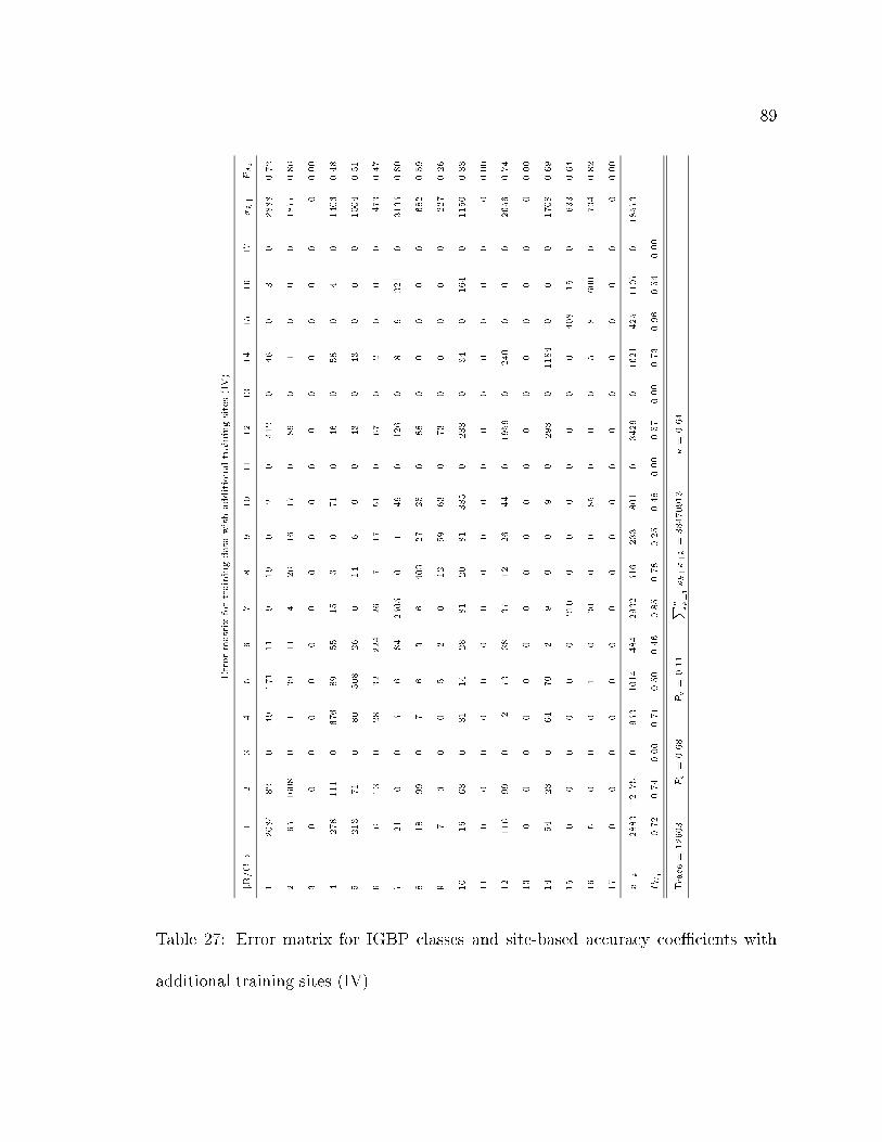
89

Errormatrixfortrainingdatawithadditionaltrainingsites(IV)

#R/C!

1

2

3

4

5

6

7

8

9

10

11

12

13

14

15

16

17

xk+

PAi

1

2084

82

0

49

171

11

9

19

0

2

0

412

0

46

0

3

0

2888

0.72

2

65

1608

0

1

39

11

4

26

16

17

0

89

0

1

0

0

0

1877

0.86

3

0

0

0

0

0

0

0

0

0

0

0

0

0

0

0

0

0

0

0.00

4

278

111

0

676

89

55

15

3

0

71

0

46

0

58

0

4

0

1406

0.48

5

213

71

0

80

508

26

0

14

6

0

0

43

0

43

0

0

0

1004

0.51

6

6

13

0

28

32

224

26

7

17

51

0

67

0

2

0

0

0

473

0.47

7

21

0

0

5

6

84

2505

0

1

49

0

126

0

8

9

321

0

3135

0.80

8

18

99

0

7

6

3

6

403

27

25

0

88

0

0

0

0

0

682

0.59

9

7

6

0

0

5

2

0

12

59

63

0

73

0

0

0

0

0

227

0.26

10

16

63

0

31

14

28

81

20

81

385

0

233

0

34

0

164

0

1150

0.33

11

0

0

0

0

0

0

0

0

0

0

0

0

0

0

0

0

0

0

0.00

12

116

99

0

12

73

38

37

12

26

44

0

1959

0

240

0

0

0

2656

0.74

13

0

0

0

0

0

0

0

0

0

0

0

0

0

0

0

0

0

0

0.00

14

54

23

0

64

70

2

9

0

0

9

0

293

0

1184

0

0

0

1708

0.69

15

0

0

0

0

0

0

210

0

0

0

0

0

0

0

408

15

0

633

0.64

16

5

0

0

0

1

0

30

0

0

85

0

0

0

5

8

600

0

734

0.82

17

0

0

0

0

0

0

0

0

0

0

0

0

0

0

0

0

0

0

0.00

x+k

2883

2175

0

953

1014

484

2932

516

233

801

0

3429

0

1621

425

1107

0

18573

PUj

0.72

0.74

0.00

0.71

0.50

0.46

0.85

0.78

0.25

0.48

0.00

0.57

0.00

0.73

0.96

0.54

0.00

Trace=12603

Po

=

0.68

Pc

=

0.11

Pq k=1

xk+

x+k

=38470913

�

=

0.64

Table 27: Error matrix for IGBP classes and site-based accuracy coe�cients with

additional training sites (IV).

90

Errormatrixfortrainingdatawithproportionalsampling(V)

#R/C!

1

2

3

4

5

6

7

8

9

10

11

12

13

14

15

16

17xk+

PAi

1

2434

74

0

101

180

9

10

3

16

14

0

27

0

19

1

0

0

2888

0.84

2

27

451

0

0

14

1

4

28

11

10

0

9

0

2

0

0

0

557

0.81

3

0

0

0

0

0

0

0

0

0

0

0

0

0

0

0

0

0

0

0.00

4

73

99

0

973

67

48

31

5

0

39

0

7

0

56

0

8

0

1406

0.69

5

271

32

0

106

458

42

5

4

4

3

0

54

0

25

0

0

0

1004

0.46

6

11

12

0

34

19

189

5

9

83

49

0

62

0

0

0

0

0

473

0.40

7

16

0

0

16

4

34

801

817

5

254

0

6

0

19

50

21

0

2043

0.39

8

24

91

0

3

17

4

5

429

26

25

0

56

0

2

0

0

0

682

0.63

9

7

10

0

0

5

29

2

10

92

18

0

13

0

0

0

0

0

186

0.49

10

18

63

0

47

14

29

120

12

74

609

0

110

0

25

0

29

0

1150

0.53

11

0

0

0

0

0

0

0

0

0

0

0

0

0

0

0

0

0

0

0.00

12

32

19

0

4

20

27

13

11

18

53

0

261

0

99

0

0

0

557

0.47

13

0

0

0

0

0

0

0

0

0

0

0

0

0

0

0

0

0

0

0.00

14

39

10

0

66

55

3

10

4

0

7

0

101

0

634

0

0

0

929

0.68

15

0

0

0

0

0

0

7

0

0

0

0

0

0

0

562

64

0

633

0.89

16

6

0

0

0

0

0

38

0

0

124

0

0

0

5

16

545

0

734

0.74

17

0

0

0

0

0

0

0

0

0

0

0

0

0

0

0

0

0

0

0.00

x+k

2958

861

0

1350

853

415

1051

1332

329

1205

0

706

0

886

629

667

0

13242

PUj

0.82

0.52

0.00

0.72

0.54

0.46

0.76

0.32

0.28

0.51

0.00

0.37

0.00

0.72

0.89

0.82

0.00

Trace=8438

Po

=

0.64

Pc

=0.11

Pq k=1xk+

x+k

=18579720

�

=0.59

Table 28: Error matrix for IGBP classes and site-based accuracy coe�cients for

proportional sampling (V).

91

ArealComparisonofUMDandBUmapinIGBPscheme

BU!

1

2

4

5

6

7

8

9

10

12

16

Total

PCi

#UMD

1

1385316

13722

185728

155501

5802

181328

84878

6884

29202

171261

21062

2240684

61.8%

2

48527

154835

2106

71081

2412

4859

16700

4757

16600

12587

1652

336116

46.1%

4

46856

73969

305819

84923

730

9048

15780

1872

25116

186921

2007

753041

40.6%

5

268495

5183

298802

141310

1307

63053

23296

783

15905

295515

15942

1170945

12.5%

6

30183

1302

15672

4604

66288

691290

300417

9040

94618

248476

82204

1589447

4.3%

7

9449

21

159900

343

19585

2160696

78013

588

110747

85964

296910

2922216

73.9%

8

1098828

42658

269229

258276

46098

258893

389455

94259

138578

475822

20443

3092539

12.6%

9

425311

37694

222658

163857

138116

379342

389795

126403

194052

764514

28855

3111528

4.4%

10

98885

8230

34971

22533

81779

305998

122217

36980

214042

598352

59101

1583088

13.5%

12

56867

17912

69222

43376

34204

214789

46931

31521

119056

815392

12664

1461934

55.8%

16

21

0

5220

0

8

774368

68

1

110

241

1617459

2397496

67.5%

Total

3468738

355526

1569327

945804

396329

5043664

1467550

313088

958026

3655045

2158299

PCj

39.9%

3.6%

19.5%

14.9%

16.7%

42.8%

26.5%

40.4%

22.3%

22.3%

74.9%

Totalpixels=20331396

Overallagreement=36.3%

Table 29: Pixel-based comparison of UMD and BU maps in the IGBP scheme.

92

ArealComparisonofUMDandEDCmapinIGBPscheme

EDC!

1

2

4

5

6

7

8

9

10

12

16

Total

PCi

#UMD

1

1475583

5755

63780

656089

16743

1360

15430

842

7409

19038

124

2262153

65.2%

2

50142

153551

435

44776

3

46

3501

3485

11450

56214

5

323608

47.4%

4

38255

98151

324741

212453

1375

22

716

740

7299

34731

0

718483

45.2%

5

282721

2935

238753

580452

5540

226

3195

189

433

9806

7

1124257

51.6%

6

22003

0

74476

95744

79565

327081

449075

5343

285121

14584

113304

1466296

5.4%

7

284

0

456

55685

29236

1257460

240405

174

52138

4829

1307154

2947821

42.7%

8

1233402

50651

345829

715377

159932

13524

182368

10713

52118

201328

11578

2976820

6.1%

9

451056

36932

324148

379340

179208

70031

449741

25695

245613

470994

18135

2650893

1.0%

10

110098

1607

23574

86279

105152

246162

131203

6824

792029

141670

2929

1647527

48.1%

12

73403

5079

91919

27893

2828

9480

95523

19689

205130

898985

21

1429950

62.9%

16

0

0

0

44

0

381328

34

0

0

61

2018003

2399470

84.1%

Total

3736947

354661

1488111

2854132

579582

2306720

1571191

73694

1658740

1852240

3471260

PCj

39.5%

43.3%

21.8%

20.3%

13.7%

54.5%

11.6%

34.9%

47.7%

48.5%

58.1%

Totalpixels=19947278

Overallagreement=38.8%

Table 30: Pixel-based comparison of UMD and EDC maps in the IGBP scheme.

93

ArealComparisonofBU

andEDCmapinIGBPscheme

EDC!

1

2

4

5

6

7

8

9

10

11

12

14

15

16

Total

PCi

#BU

1

2878390

18737

38227

406213

22532

932

21405

5082

8425

2998

48686

17111

0

0

3468738

83.0%

2

29337

175851

4360

13721

323

99

7462

3458

22522

2170

65290

30933

0

0

355526

49.5%

4

86811

2682

915706

291041

5450

180675

66468

1440

5534

9

7441

6070

0

0

1569327

58.4%

5

316191

70461

97734

236556

19164

242

51990

3858

14881

592

98386

35749

0

0

945804

25.0%

6

32585

1841

26025

11529

1076

43479

91533

2062

117367

3223

55370

10239

0

0

396329

0.3%

7

37369

633

157155

261646

296634

1053231

745072

457

230055

1422

144100

150013

162480

1803397

5043664

20.9%

8

45048

27674

18965

682215

22157

37835

256689

3882

39864

231720

49001

52500

0

0

1467550

17.5%

9

41029

6078

21421

42585

4984

522

49859

8103

22851

3618

44700

67338

0

0

313088

2.6%

10

27607

30537

51897

75971

64214

169949

86648

23451

202092

9219

68496

147945

0

0

958026

21.1%

11

0

0

0

0

0

0

0

0

0

0

0

0

0

0

0

0.00%

12

125078

16722

101135

619864

99757

156570

158232

19259

646445

97030

960257

654696

0

0

3655045

26.3%

14

113581

448

39861

168355

29709

114555

32573

1066

341511

4746

301841

335328

0

0

1483574

22.6%

15

0

0

0

0

0

73642

646

0

0

0

15

0

1308142

172794

1555239

84.1%

16

3921

2997

15625

44436

13582

474923

2614

1576

7193

2961

8657

2217

0

22358

603060

3.7%

Total

3736947

354661

1488111

2854132

579582

2306654

1571191

73694

1658740

359708

1852240

1510139

1470622

1998549

PCj

77.0%

49.6%

61.5%

8.3%

0.2%

45.7%

16.3%

11.0%

12.2%

0.0%

51.8%

22.2%

89.0%

1.1%

totalpixels=

21814970

Overallagreement=

38.3%

Table 31: Pixel-based comparison of BU and EDC maps in the IGBP scheme.

94

Areal Comparison of UMD and EDC map in biome scheme

EDC! 1 2 3 4 5 6 7 Total PCi

#UMD

1 792029 246162 141670 138027 216612 110098 2929 1647527 48.1%

2 52138 1257460 4829 240579 85377 284 1307154 2947821 42.7%

3 205130 9480 898985 115212 127719 73403 21 1429950 62.9%

4 297731 83555 672322 668517 2191417 1684458 29713 5627713 11.9%

5 304303 327375 115335 466244 1912950 393121 113316 3632644 52.7%

6 7409 1360 19038 16272 742367 1475583 124 2262153 65.2%

7 0 381328 61 34 44 0 2102542 2484009 84.6%

Total 1658740 2306720 1852240 1644885 5276486 3736947 3555799

PCj47.7% 54.5% 48.5% 40.6% 36.3% 39.55% 59.1%

Total pixels = 20031817 Overall agreement = 45.5%

Table 32: Pixel-based comparison of UMD and EDC maps in the biome scheme.

95

Areal Comparison of UMD and BU map in biome scheme

BU! 1 2 3 4 5 6 7 total PCi

#UMD

1 652144 176637 53541 153166 33515 357383 221141 1647527 39.6%

2 151806 2461179 2014 26648 63532 47257 195385 2947821 83.5%

3 520201 21282 358357 208611 123468 136137 61894 1429950 25.1%

4 1097453 364515 328838 694396 535548 2341016 265947 5627713 12.3%

5 562538 726865 161065 239013 1017841 708270 217052 3632644 28.0%

6 201336 105241 125620 65614 110138 1636584 17620 2262153 72.3%

7 24457 681678 9845 15218 11015 10880 1730916 2484009 69.7%

Total 3686851 4896929 1378206 1847457 2006770 5337426 2748025

PCj20.3% 54.2% 34.5% 49.5% 53.7% 31.2% 63.9%

Total pixels = 20031817 Overall agreement = 42.7%

Table 33: Pixel-based comparison of UMD and BU maps in the biome scheme.

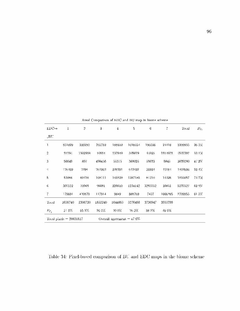
96

Areal Comparison of EDC and BU map in biome scheme

EDC! 1 2 3 4 5 6 7 Total PCi

#BU

1 851029 239292 705732 188682 1010254 190536 24410 3209935 26.5%

2 81794 1502988 10884 737049 345679 44025 1814978 4537397 33.1%

3 56649 897 490456 55375 368025 58033 9845 1039280 47.2%

4 126469 2294 261062 328291 612432 56934 15184 1402666 23.4%

5 55986 69410 168111 105829 1397185 84210 14326 1895057 73.7%

6 307122 70969 98081 220610 1234142 3295752 10851 5237527 62.9%

7 179691 420870 117914 9049 308769 7457 1666205 2709955 61.5%

Total 1658740 2306720 1852240 1644885 5276486 3736947 3555799

PCj51.3% 65.2% 26.5% 20.0% 26.5% 88.2% 46.9%

Total pixels = 20031817 Overall agreement = 47.6%

Table 34: Pixel-based comparison of BU and EDC maps in the biome scheme.

97

Figure 5: Supervised classi�cation of IGBP classes for North America.

98

Figure 6: Supervised classi�cation of biome classes for North America.

99

Figure 7: Map comparison in the biome scheme between EDC and BU.

100

Figure 8: Map comparison in the biome scheme between UMD and BU.