box modeling: unsteady, uniform conservation of mass
TRANSCRIPT

CHAPTER
3
Box Modeling: Unsteady, Uniform Conservation of Mass
We start our discussion of model derivations with systems that are best considered in terms of macroscopic control volumes, or “boxes”; that is, large reservoirs of mass or energy that are effectively homogeneous (well mixed) and evolve in time in response to imbalances between input and output. A familiar example is the global carbon cycle, which one typically envisions as a set of carbon reservoirs, ocean, atmosphere, living organisms, sediments, soils, and sedimentary rocks, among which carbon is transferred by a host of physical and biological processes. In such prob-lems we are generally uninterested in spatial distributions within the reservoirs, although we may wish to study the coupled response of many such reservoirs to internally or externally driven perturbations. In the case of the carbon cycle, we may wish to separate the global ocean into sur-face, deep, and high- latitude boxes; if we do, however, we must specify the water fluxes that advect carbon from one oceanic reservoir to the next.
Consideration of conservation of mass or energy in systems of reservoirs leads to a set of coupled ordinary differential equations. The process of constructing and solving such systems is often called box modeling. In this chapter, we describe the process of box modeling through a number of examples, including an assessment of the controls on the radiocarbon content of the biosphere, a

40 • Chapter 3
simplified version of the global carbon cycle, a method for interpreting excursions in the carbon isotopic composition of the ocean in deep time, and a simple climate model. Along the way we will introduce the important concepts of residence and response time, steady state, coupled systems, and nonlinear systems. We then present methods for the solution of the ODEs that arise. For further examples and an alternative introduction to box modeling for geochemi-cal cycles, see Walker (1991).
Translations
Example I: Radiocarbon Content of the Biosphere as a One- Box Model
Physical PictureCosmic ray bombardment of the atmosphere leads to
the production of radioactive 14C from the abundant 14N nucleus. The rate of production thus varies as a function of the cosmic- ray neutron flux to the atmosphere, which varies in time, and the abundance of nitrogen, which is effectively constant over the time scales of interest (millen-nia). 14C is radioactive and thus is lost from its Earth sur-face reservoirs through radioactive decay. Radiocarbon’s abundance, M, is often characterized in terms of “radio-carbon units” (RCU = 1026 14C atoms). Accordingly, the rate of decay (D) and the rate of production (P) are ex-pressed in units of RCU y−1. Radiocarbon produced in the atmosphere rapidly combines with oxygen to form CO2 and then gets photosynthesized or stirred into the ocean; most radiocarbon (92%) resides in the deep ocean. We de-fine the biosphere (after Vernadsky, 1997 reprint) as the atmosphere, ocean, and living and decomposing biomass. The radiocarbon content of the biosphere, M, can be mod-eled with a box model (fig. 3.1).
Physical LawsRadiocarbon decays with a known rate that is linearly
proportional to its abundance (fig. 3.2), that is,

Box Modeling • 41
,DdtdM kM= = − (3.1)
where the minus sign indicates decay, and k is the decay constant (k = 1.209 10−4 y−1). If a sample is isolated from its source of production, for example, when photosynthe-sis by a cotton plant leads to incorporation of radiocarbon into the cotton, equation 3.1 can be integrated to yield
,eM M kt0= − (3.2)
where M0 is the initial amount of radiocarbon in the sample (RCU), and t is the time (in years). This equation
Rate of production(P; RCU y–1 )
Rate of decay(D; RCU y–1 )
Radiocarbon contentof the biosphere
M (RCU)
Figure 3.1. Radiocarbon balance for the biosphere; M changes with time in response to imbalances between rate of produc-tion, P, and rate of decay, D.
Time (thousands of years)
Perc
ent R
emai
ning
100
80
60
20
40
00 5 10 15 20 25
Figure 3.2. Decay of an initial amount of radiocarbon isolated from the atmospheric source. The half- life (the time it takes for half of the material to decay), 5,730 years, is shown.

42 • Chapter 3
indicates that the radiocarbon content simply decreases with time according to the well- known exponential decay law. Our ODE and its solution will be a bit more compli-cated because of the continuous production term P.
Restrictive AssumptionsWe are assuming that the biosphere is homogeneous
with respect to its radiocarbon content and that all other processes in the carbon cycle are either unimportant or balanced so that we can justifiably focus on the balance between production via cosmic rays and consumption via radioactive decay. For now, also assume that the rate of production is constant in time. Finally, we acknowledge that decay rate constants are constant in time and indepen-dent of any other physical condition of the environment.
Perform the BalanceHaving defined the processes that introduce or remove
radiocarbon from the atmosphere, we can perform the mass balance, first in words, and then symbolically. We write:
TROCM MRI MRO SOURCE/SINK.= − +
TROCM is shorthand for “the time rate of change of mass in the control volume” (in our case, a macroscopic reser-voir of mass), MRI stands for “mass rate into the control volume,” and MRO stands for “mass rate out.” Sources and sinks reflect any internal production and destruction. In this example, there is no transport in or out of radio-carbon, so we only have internal sources and sinks.
The time rate of change of mass of radiocarbon in the biosphere is equal to the source (production by cosmic rays from nitrogen) minus the sink (radioactive decay):
.dtdM P D
P kM
= −
= − (3.3)
Check UnitsAll terms in the equation above are expressed in units
of RCU y–1.

Box Modeling • 43
Define Interval, Specify Initial and Boundary ConditionsFor time- dependent ODEs (even systems of ODEs),
we only need to provide initial conditions, because there are no explicit spatial boundaries to the reservoirs. We do have to provide initial conditions for each reservoir being simulated. In this case, for heuristic purposes, we could consider a biosphere that is suddenly exposed to cos-mic rays, with an initial biospheric radiocarbon content of zero, so that we could observe its temporal evolution toward a constant value consistent with modern rates of production and its known decay constant.
A reservoir is said to be in steady state, that is, un-changing in time, when its inputs and outputs are balanced:
0.dt
dM input rate output rate= − = (3.4)
In this case, at steady state:
0.dt
dM P kM= − = (3.5)
Rearranging terms, we can solve for the steady- state radio-carbon abundance of the biosphere, Mss:
.MkPss = (3.6)
The abundance of radiocarbon (and any radionuclide with a simple production and decay scheme as shown here) at steady state is thus directly proportional to production rate and inversely proportional to its decay constant.
Often in modeling global cycles of the elements, we use the concept of steady state to estimate terms in the mass balance that are otherwise difficult to measure. For example, in this case we could use the measured abun-dance of radiocarbon in the biosphere and the known decay constant for radiocarbon to determine its average production rate. So, for a steady- state abundance Mss = 20,300 RCU and a decay constant of 1.209 10–4 y–1, equation 3.6 yields a production rate P = 2.45 RCU y–1 (Lassey and Enting, 1996).

44 • Chapter 3
There is a known analytic solution to equation 3.5 for a specified initial condition, M0:
.MkP
kP M e kt0= − − −d n (3.7)
Note that as
, .t MkP Mss" "3 = (3.8)
Thus, the system evolves to the steady state predicted on the basis of a balance between input and output (fig. 3.3). The characteristic time it takes for an initial perturbation from steady state (M 0 M ss) to diminish (i.e., its response time) can be characterized by 1/k (the inverse of the decay constant, expressed in years). For exponentially decaying reservoirs, the response time is sometimes referred to as the e- folding time, because it is the time it takes for the perturbation to diminish by a factor of e–1, or ~37% of its initial value.
Figure 3.3. The growth of the radiocarbon content of the atmosphere from an initially depleted atmosphere, expressed in e- folding times. For radiocarbon, the e- folding time (1/k) is 8,271 years.
e-Folding Times
M (%
of s
tead
y st
ate)
100
80
60
20
40
00 1 2 3 4 5

Box Modeling • 45
For reservoirs at steady state, one can determine the av-erage amount of time a unit of material spends in the reser-voir by dividing the reservoir size by either the input or the output (because they are equal at steady state). The result is referred to as the residence time (t). In the case above,
.P
Mk1ss
/ τ= (3.9)
Note here that the residence and response times are the same. This is not generally true, especially for reservoirs that have multiple inputs and outputs. In such cases, the residence time can only be defined with respect to a par-ticular input or output, and the response time is different from any of these residence times.
Periodic ForcingA more interesting situation arises if the input to the
reservoir varies in time (Holland, 1978). For example, the radiocarbon production rate varies periodically in time with the sunspot cycle (11- year period). We can represent this with a production rate function that varies about our canonical value of P = 2.45 RCU y–1 with an amplitude b = 1 RCU and a frequency
112ω π= (3.10)
as
( ),sinP P b tω= +l (3.11)
where t is time in years. The differential equation is now:
( ) ,sindt
dM P b t kMω= + −l (3.12)
which has an analytic solution (for an initial value of M0)
( ) .sin
MkP
kP M
kb e
k
b t
kt02 2
2 2
ωω
ωω δ
= − − −+
++
−
−l ld n (3.13)
46 • Chapter 3
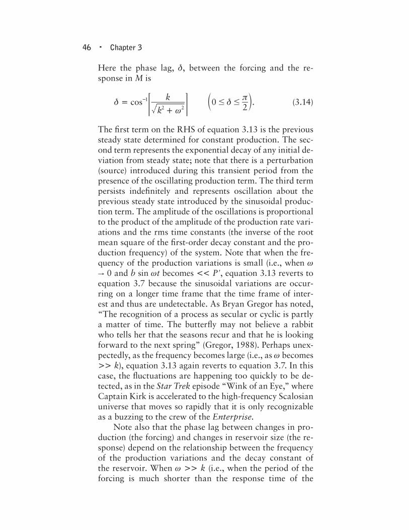
Here the phase lag, , between the forcing and the re-sponse in M is
.cosk
k 022 2
1 # #δω
δ π=+
− c mf p (3.14)
The first term on the RHS of equation 3.13 is the previous steady state determined for constant production. The sec-ond term represents the exponential decay of any initial de-viation from steady state; note that there is a perturbation (source) introduced during this transient period from the presence of the oscillating production term. The third term persists indefinitely and represents oscillation about the previous steady state introduced by the sinusoidal produc-tion term. The amplitude of the oscillations is proportional to the product of the amplitude of the production rate vari-ations and the rms time constants (the inverse of the root mean square of the first- order decay constant and the pro-duction frequency) of the system. Note that when the fre-quency of the production variations is small (i.e., when w " 0 and b sin wt becomes << P , equation 3.13 reverts to equation 3.7 because the sinusoidal variations are occur-ring on a longer time frame that the time frame of inter-est and thus are undetectable. As Bryan Gregor has noted, “The recognition of a process as secular or cyclic is partly a matter of time. The butterfly may not believe a rabbit who tells her that the seasons recur and that he is looking forward to the next spring” (Gregor, 1988). Perhaps unex-pectedly, as the frequency becomes large (i.e., as w becomes >> k), equation 3.13 again reverts to equation 3.7. In this case, the fluctuations are happening too quickly to be de-tected, as in the Star Trek episode “Wink of an Eye,” where Captain Kirk is accelerated to the high- frequency Scalosian universe that moves so rapidly that it is only recognizable as a buzzing to the crew of the Enterprise.
Note also that the phase lag between changes in pro-duction (the forcing) and changes in reservoir size (the re-sponse) depend on the relationship between the frequency of the production variations and the decay constant of the reservoir. When w >> k (i.e., when the period of the forcing is much shorter than the response time of the

Box Modeling • 47
reservoir), the reservoir responds with a phase lag of p/2, or a quarter phase lag of the period of the forcing. This is the maximum lag possible between forcing and response in a simple, linear system (Richter and Turekian, 1993). For sinusoidal forcing, this means that the reservoir responds with its first derivative to the forcing (i.e., it increases most rapidly when the forcing has the largest positive value, and vice versa). In contrast, when the period of the forcing is long with respect to the response time of the reservoir, the phase lag is 0; the reservoir rises and falls in concert with the forcing.
So, in the case of radiocarbon in the biosphere, sun-spot cycles (11- year period) have a significant effect on production rates but, once the transient effect of impos-ing a sinusoidal production term has vanished, we are left with a barely noticeable effect on the radiocarbon abun-dance (fig. 3.4). The radiocarbon abundance responds as predicted with its first derivative to the forcing.
Time (y)
Periodic Production120
100
80
60
20
40
0
5
4
3
1
2
00 10 20 30
M (% of steady state)P (RCU per year)
P (R
CU p
er y
ear)
M (%
of s
tead
y st
ate)
40 50
Figure 3.4. Response of the radiocarbon abundance of the atmosphere (left ordinate, expressed as a percentage of the average steady- state abundance) to the 11- year sunspot cycle, presuming an amplitude of 1 RCU to the variation in produc-tion rate (right ordinate).

48 • Chapter 3
Example II: The Carbon Cycle as a Multibox Model
In the example above, only one reservoir was considered —the radiocarbon content of the atmosphere. More com-monly, we are interested in the transfer of matter or energy between two or among multiple reservoirs. In such cases, we end up with a system of coupled ordinary differential equations. Here we explore two example cases, one of matter transfer (the global carbon cycle) and another of energy transfer (a simple 1- D climate model).
Physical PictureFor simplicity, we begin by considering an isolated part
of the global carbon cycle, one that involves only two res-ervoirs, the atmosphere and the living biomass (after Hol-land, 1978). The atmosphere contains carbon in the form of gaseous carbon dioxide, whereas living biomass contains carbon in multiple organic forms. Let’s call the amount of carbon in the atmosphere and the biomass M1 and M2, re-spectively, with units of gigatons (1015 g) of carbon. F12, the flux of carbon from reservoir 1 to 2 due to photosynthesis, removes carbon from the atmosphere and incorporates it into biomass. During respiration and decomposition (F21), the carbon is returned to the atmosphere. The rates of these processes can be expressed in gigatons carbon per year (GtC y–1). If we assume homogeneity in these two res-ervoirs, we can represent this carbon cycle as a box model with two boxes, coupled by two transfers (fig. 3.5).
It is clear from this diagram that the cycle is closed: carbon is recycled between the two reservoirs but is nei-ther added to nor lost from the system (a gross simplifica-tion, of course).
Physical LawsFor this simple consideration, let’s assume that the rate
of removal of carbon from each reservoir is simply propor-tional to its mass, as in the first example. In other words, the rate of photosynthesis is
,F kM12 1 1= (3.15)

Box Modeling • 49
and the rate of respiration and decomposition is
F21 = k2M2. (3.16)
Here, k1 is the rate constant for photosynthesis, and k2 is the rate constant for respiration and decay, both in units of y–1. We can estimate these rate constants by setting up a steady- state model with specified reservoir sizes and fluxes. Some representative values for today are M1 = 800 GtC, M2 = 600 GtC, and F12 = F21 = 60 GtC y–1. With these values, k1 becomes 0.075 y–1 and k2 becomes 0.1 y–1. The residence time for reservoir 1 (t1) is 1/k1 = 13.3 years and for reservoir 2 (t2) is 1/k2 = 10 years. It’s a remark-able fact that the biota process the entire mass of C in the atmosphere in a matter of decades.
Restrictive AssumptionsWe are assuming that the atmosphere and biomass are
homogeneous in their carbon content and that all other processes in the carbon cycle are either unimportant or balanced so that we can justifiably focus on the balance between photosynthesis and respiration/decomposition.
Perform the BalanceStated in words, the time rate of change of mass of car-
bon in the atmosphere is equal to the mass rate in (through respiration and decay) minus the mass rate out (through photosynthesis), or
.dt
dMF F
k M k M
121 12
21 2 12 1
= −
= − (3.17)
Rate of photosynthesis(F12; GtC y–1 )
Rate of respiration and decay(F21; GtC y–1 )
Carbon contentof the atmosphere
M1 (GtC)
Biomass
M2 (GtC)
Figure 3.5. Simple representation of the exchange of carbon between the global living biomass and the atmosphere.

50 • Chapter 3
The time rate of change of mass of carbon in the biomass is simply the negative of equation 3.17, which of course it must be, as we are treating this as a closed system:
.dt
dMF F
k M k M
21
12 1 21
212
2
= −
= − (3.18)
Check UnitsAll terms in the equation above are expressed in units
of GtC y–1.
Define Interval, Specify Initial and Boundary ConditionsHere we have two ODEs, so we need to provide initial
conditions for M1 and M2. Let’s assume that at some time (say during an asteroid impact), half of the carbon origi-nally in the biomass is transferred instantaneously to the atmosphere (i.e., 1M1
0 = ,100 GtC and 300M20 = GtC).
Under these ICs , the simple, linear, coupled system of equations (equation 3.17 and equation 3.18) has analytic solutions:
Mk k
k M Mk k
k M k Me ( )t k k t
112 21
21 10
20
12 21
12 10
21 20
12 21=++
++− − +_ i
and
.Mk k
k M Mk k
k M k Me ( )t k k t
12 21
12 10
20
12 21
12 10
21 20
212 21=
++
+−
− − +_ iNotably, now the response time is 1/(k1 + k2), which in our case is 1/(0.075 + 0.1) = 5.71 years (fig. 3.6). Thus, by coupling the two reservoirs, the response time has become shorter than the residence time of either reservoir. This tells us that it is unwise to use residence times as an indi-cator of reservoir response in even slightly complex box models.
One may argue that it would be more reasonable to specify that the photosynthetic rate depends not only on the atmospheric carbon content but also on the amount of biomass itself. In other words, we might want to express F12 as:

Box Modeling • 51
.F k M M12 12 1 2= (3.19)
The rates of change of the two reservoirs now become
dtdM
k M k M M2 21
21 12 1= − (3.20)
and
.dt
dMk M M k M212 1 2 21 2= − (3.21)
Note that k12 no longer has intuitive units (GtC–1 y–1). Find-ing analytic solutions for nonlinear systems of equations is difficult, and often impossible. In the next chapter, we will explore numerical solutions to nonlinear ordinary differ-ential equations. Here we simply present the results of the numerical integration (fig. 3.7). Note the interesting dif-ference between this result and the previous simulation of the linear system. Now the response time is considerably
Figure 3.6. Response of the linear C cycle to an initial transfer of 300 GtC from the biomass to the atmosphere. Note that the perturbation from steady state has an e- folding time of 5.7 years, the calculated response time of the system (see text).
Time (y)
1200
1000
800
600
200
400
00 5 10 15
M1M2
20 25
Gto
ns C

52 • Chapter 3
longer (~23 years) than that calculated for the linear system (5.7 years) or for either reservoir’s residence time (10–13 years). This extended response time arises because one of the two fluxes is sensitive to both reservoirs. Whereas in the linear model the flux from the atmosphere to the biomass increased to more than 80 GtC y−1 immediately after the transfer of 300 GtC to the atmosphere, here it decreased from the steady- state value of 60 GtC y−1 to just slightly over 40 GtC y−1, much closer to the rate of trans-fer of C from the biomass to the atmosphere (30 GtC y−1), which has been reduced to half the original steady- state value with a halving of the biomass reservoir. The reser-voirs evolve back to steady state more slowly then, respond-ing to this much smaller flux imbalance between input and output for each reservoir. In general, if the fluxes are de-pendent on both reservoir sizes in a coupled system such as this, and if the residence times of the two reservoirs is vastly different, the response time can greatly exceed either of the two residence times (cf. Rothman et al., 2003).
Figure 3.7. Response of the nonlinear C cycle to the sudden transfer of 300 GtC from the biomass to the atmosphere. Con-trast with response of linear system in figure 3.6.
Time (y)
Gto
ns C
1200
1000
800
600
200
400
00 25 50 75
M1M2
100

Box Modeling • 53
Example III: One- Dimensional Energy Balance Climate Model
Most serious climate modeling is done on supercomputers that solve large systems of partial differential equations simultaneously. However, “toy” climate models, the sort that can easily run on your PC, are sometimes of use in exploring the basics of climate system operation. One ver-sion of a toy climate model treats Earth’s surface energy as being enclosed in a series of reservoirs that encircle the earth but extend a finite distance in latitude. These “zonal” reservoirs are linked by the exchange of energy between adjacent reservoirs. Although we said above that transport modeling is typically not appropriately treated with box models, in cases like this, where we can specify that the transport of material or energy is dependent on reservoir size, box modeling can be performed. In this example, we draw heavily on the model description by Walker (1991).
Physical PictureIn our one- dimensional energy balance climate model,
we separate the earth surface into n zonal bands (180/n) degrees wide spanning from pole to pole (fig. 3.8). Each of these reservoirs contains heat energy, characterized by its temperature. When we go to solve this problem, we will need to remember that the volume of each reservoir di-minishes with the cosine of latitude, as do the boundaries between adjacent reservoirs across which they exchange en-ergy. Energy is received from the sun at all latitudes, and a fraction (the albedo, a) is reflected back to space. Each reser-voir radiates heat to space, and the efficiency of this transfer depends on atmospheric composition (i.e., the greenhouse effect). Temperature differences between adjacent reservoirs drives heat transfer (generally from equator to pole).
Physical LawsEnergy input into each box j (Fin,j), typically in units of
W m–2, is calculated as the product of the solar constant (S) and the fraction of this energy absorbed (not reflected, i.e., 1 a):

54 • Chapter 3
(1 ) .F S ain #= − (3.22)
Note that both S and a are functions of latitude because of variations in average solar angle and differences in land and cloud cover. With simple climate models such as pre-sented here, these values are typically constants obtained from the literature. Outgoing radiation is calculated ac-cording to the Stefan–Boltzmann law of blackbody radia-tion; that is,
,F T j4
ou t εσ= (3.23)
where s is the Stefan–Boltzmann constant (5.67 10–8 W m–2 K–4), and e is the emissivity (i.e., the efficiency with which the surface is able to emit radiation to space). The
Figure 3.8. Gridded representation of the global climate system. We divide Earth into latitudinal zones of width dx and perform an energy balance for each macroscopic control volume. Note that the circumference of the boundaries between adjacent zones ( ) diminish with the cosine of latitude.
x
dx Tj
Tj–1
Tj+1λj,j+1
Box Modeling • 55
emissivity diminishes as the greenhouse effect intensifies (i.e., as CO2 and other greenhouse gases accumulate in the atmosphere).
The transfer of heat energy from one reservoir to the next occurs as a result of complicated processes of atmo-spheric circulation. For our purpose, we will assume that the first- order rate law called Fourier’s law applies here; that is, that the heat transfer is proportional to the temper-ature difference between adjacent reservoirs and inversely proportional to the distance between the (centers of) the two reservoirs:
.F Ddx
T TC, ,x j j
j jp1
1 ρ= −−
−− (3.24)
Here, D is the proportionality constant (in units of m2 s–1), which, when multiplied by the density (r; kg m–3) and heat capacity (Cp; J K
–1 kg–1) relates the energy flux (in W m–2) to the temperature gradient. The distance between the cen-ters of the boxes is dx, and T is temperature in Kelvin (K). One typically calculates the heat capacity of each zonal reservoir based on the relative proportions of land and sea in that zone and their different heat capacities.
Restrictive AssumptionsThis simple climate model ignores a host of processes
that affect Earth’s climate. In keeping the albedo con-stant in each box we ignore any and all feedbacks associ-ated with changing cloud, ice, and vegetation cover. The heat transfer relationship we adopted basically ignores all transfers associated with the general circulation of the atmosphere and with the advection of latent heat (water vapor) by the winds. We also ignore the important effects of topography and other factors that vary longitudinally. The results we obtain can only be interpreted in terms of the model’s very basic representation of meridional gradi-ents in temperature.
Perform the BalanceThe time rate of change of energy in each reservoir is
the difference in the rates of input and output of energy

56 • Chapter 3
from each reservoir. The energy content of each reservoir is the product of its temperature, density, heat capacity, and volume. Volume is obtained by the product of the surface area of each reservoir j (Aj) and a “radiatively active” thick-ness H, generally thought of as a depth in the ocean that exchanges heat on a seasonal timescale. The input flux of energy from the sun is through the reservoir area Aj, as is the outgoing infrared radiation Fout, but the exchange of energy across latitudinal bands (i.e., from box to box) is through a cross- sectional area that is the product of the depth H and the length of the border between the two adja-cent reservoirs, a function of latitude ( j,j−1). In other words,
( ) ( )
.dtd C HAT F F A F
F H
, ,
, , ,
p j j j x j j
x j j j j
1
1 1
in ou tρ
λ
= − +
+
−
+ +
(3.25)
Substituting the expressions for the fluxes (equation 3.22 to equation 3.24) into equation 3.25 gives:
( ) (1 )
.
dtd C HAT S a T A
Ddx
T TC H D
dxT T
C H, ,
p j j j j
j jp j j
j jp j j
4
11
11
#ρ εσ
ρ λ ρ λ
= − −
−−
−−−
−+
+
` j (3.26)
This equation can be simplified by dividing through by the factors that are independent of time (Cp, r, H, and Aj) to yield
( )(1 )
.
dtd T
C HS a T
Ddx
T TA
Ddx
T TA
4,
,
jp
j j j
j
j j
j j
j
j j
1 1
1 1
#
ρεσ λ
λ
=− −
−−
−−
− −
+ +
` j (3.27)
Check UnitsAll terms in the equation above are expressed in units
of K y−1.
Define Interval, Specify Initial and Boundary ConditionsA typical initial condition would be to specify a uni-
form temperature for all reservoirs. Temperatures would then evolve (“spin up”) toward the steady state as the

Box Modeling • 57
result of differential energy input to the various latitudes. Two boundary conditions must be satisfied. Usually, one could either specify the temperature for the two most pole-ward boxes or, recognizing that there is no flux poleward of these boxes, remove the second term on the RHS of equation 3.27 for reservoir 1 and the first term on the RHS of equation 3.27 for reservoir n.
Once these steps have been completed, we have a well- posed 1- D climate model. The system of equations is highly coupled, nonlinear, and thus not amenable to ana-lytic solution. Instead we turn to numerical solutions.
Finite Difference Solutions of Box Models
As we’ve seen in past examples, interesting and useful models of Earth systems tend to be nonlinear and highly coupled. To study these models quantitatively usually re-quires numerical solutions of the system of differential equations. In box models, we have a system of ordinary differential equations to solve beginning from a specified set of initial conditions. As discussed in chapter 2, the gen-eral approach is to convert these differential equations to algebraic equations using finite differences and then use techniques from linear algebra to solve the equations.
The Forward Euler Method
Conceptually, this approach uses the known derivative of the dependent variable (e.g., y) evaluated at an initial value (e.g., yn) to extrapolate over a finite increment of the inde-pendent variable (e.g., t). In other words,
,y ydtdy tn n
y
1
nD= ++ (3.28)
which can readily be generalized in vector notation for systems of equations representing the coupled evolution of multiple reservoirs:
,ty F y tn n
D
D= lv v_ i (3.29)

58 • Chapter 3
.y y y Fdt
dywhere andn nn
1D = − =+ lv v v v (3.30)
This approach, sometimes referred to as the forward Euler method, as well as its shortcomings, are obvious from figure 3.9.
Here it is clear that by picking a large time increment for the extrapolation, we have introduced a large error into our estimate of y at the future time. This error arises be-cause we have implicitly neglected the higher- order terms in the Taylor series approximation used in equation 3.28. If we use the forward Euler approach, we must use very small time steps to avoid large errors. The error is O(Dt), so reducing the size of Dt only provides a linear improve-ment in accuracy.
Notice that if we ignore insolation and infrared radia-tion, equation 3.27 is similar in form to the FTCS discreti-zation of the one- dimensional diffusion equation (equation 2.18). In fact, if we ignore the variation of with latitude, then A/ = dx, and we can recast the simplified version of equation 3.27 (diffusion only) as:
t
yyn
yn+1
tn
Δt
yn
dy___dt
tn+1
Estimatedsolution
Truesolution
Figure 3.9. The forward Euler method of numerical approxima-tion extrapolates the solution from a known position yn over a given interval t using the known derivative of the solution (i.e., the tangent to the solution) at that position.

Box Modeling • 59
( )
.
dtd T D
dxT T
Ddx
T T
Ddx
T T T2
jj j j j
j j j
21
21
21 1
= −−
−−
=− +
− +
− +
(3.31)
Then if we apply the forward Euler method to the solution of equation 3.31, we obtain:
.T Tx
D t T T T2jn
jn
jn
jn
jn1
2 1 1D
D= + − ++− +` j (3.32)
Equation 3.32 is indeed identical to equation 2.18. In other words, the FTCS solution scheme for the partial dif-ferential equation representing one- dimensional diffusion is the same as the forward Euler method of solving the same problem using box modeling. The difference is that in the former we treat Dx as a very small increment in x, whereas in box modeling we consider Dx to be a macro-scopic property of the system.
Predictor–Corrector Methods
We could improve on the forward Euler method if we had a way of “anticipating” the curvature of the real solution (i.e., if we could estimate the derivative of the function at a future time). If so, then we could average these two derivatives to obtain a better estimate of the slope of the solution in the interval of extrapolation; that is to say, we want
.y y dtdy
dtdy
t2
n n y y1 n n1
D= ++
+ +f p (3.33)
Of course, we don’t know dtdy
1 1n n+ +,t y , so let’s first “predict” yn+1 using Euler’s method, and then correct the value by using equation 3.33. The exponential decay equation pro-vides a simple example:
.dtdy yλ= − (3.34)
From equation 3.28,

60 • Chapter 3
(1 ) .y y y t
y t
n n n
n
1 λ
λ
D
D
= −
= −
+
(3.35)
This is the Euler predictor step for yn+1. In equation 3.33, call the derivatives two new terms, k1 and k2:
kdtdy
1 n=
y (3.36)
and
kdtdy
2 n 1=
+y (3.37)
such that
.y yk k
t2
n n1 1 2 D= +++ d n (3.38)
For example, if Dt = 1, = 0.25, and y0 = 16, then for the predictor step, using equation 3.34, y1 = 16 (1 0.25 1) = 12. We use this value to calculate k2 = 0.25 12 = 3; k1 = 0.25 16 = 4. Then for the corrector step we use equation 3.38 to improve on our previous estimate of y1:
16 ( ) 1 12.5.y2
4 31 = + − + − =c m (3.39)
This method provides an improved estimate of the actual solution; in fact, it coincidentally is the actual solution after the first time step. The method is called second- order Runge–Kutta after Carl Runge (1856–1927), a German mathematician and astronomer who has a crater on the moon named after him, and another German mathemati-cian, M. W. Kutta (1867–1944), a pioneer in the field of aerodynamics. At subsequent times the approximation is not perfect, but the accuracy is improved over the Euler method (table 3.1); it is now O(Dt2).
Higher- order Runge–Kutta methods add terms (k3, k4) that improve the accuracy even more but have addi-tional computational overhead.
Stiff Systems
We have seen that in developing box models for natural systems (e.g., the carbon cycle), we encountered reservoirs
Box Modeling • 61
coupled by exchange of material that had vastly differ-ent time constants (response or residence times). Such instances revealed interesting behaviors in terms of gen-erating much longer period responses to forcings than one would anticipate based on residence times alone.
Mathematicians refer to systems of equations with wide- ranging time constants as stiff systems. These sys-tems present particular challenges to numerical solution using the “explicit” methods discussed so far, because sta-bility constraints require that we keep our time increment Dt small with respect to the residence time of the fastest cycling reservoir. In other words, even if we are primarily interested only in the long- term behavior of the system, we must take short time steps (i.e., perform many more calculations than would seem to be necessary to study the system).
One example of a stiff system is the set of equations describing what has been called the “Rothman ocean” (Rothman et al., 2003).
Example IV: Rothman Ocean
Physical PictureConsider the following model of the oceanic carbon
cycle, including two reservoirs: one, the dissolved inor-ganic carbon reservoir (DIC; M1), and the second, a large reservoir of dissolved organic carbon (DOC; M2) thought to have characterized the Proterozoic Era ocean more than
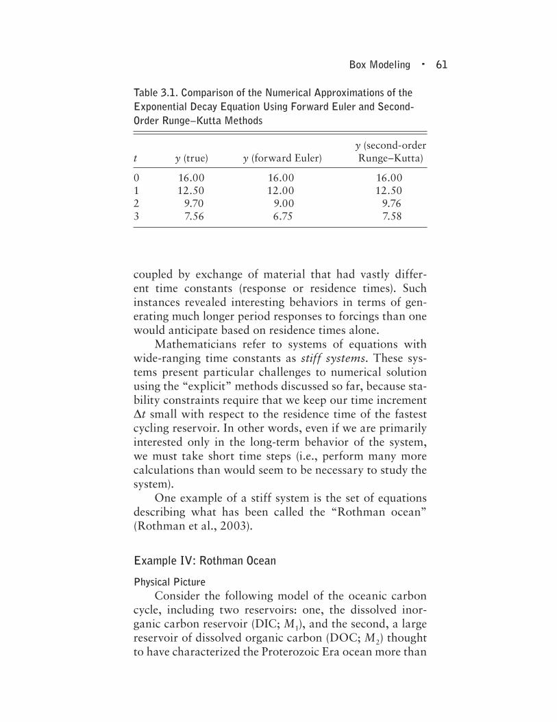
Table 3.1. Comparison of the Numerical Approximations of the Exponential Decay Equation Using Forward Euler and Second-Order Runge–Kutta Methods
y (second-ordert y (true) y (forward Euler) Runge–Kutta)
0 16.00 16.00 16.001 12.50 12.00 12.502 9.70 9.00 9.763 7.56 6.75 7.58
62 • Chapter 3
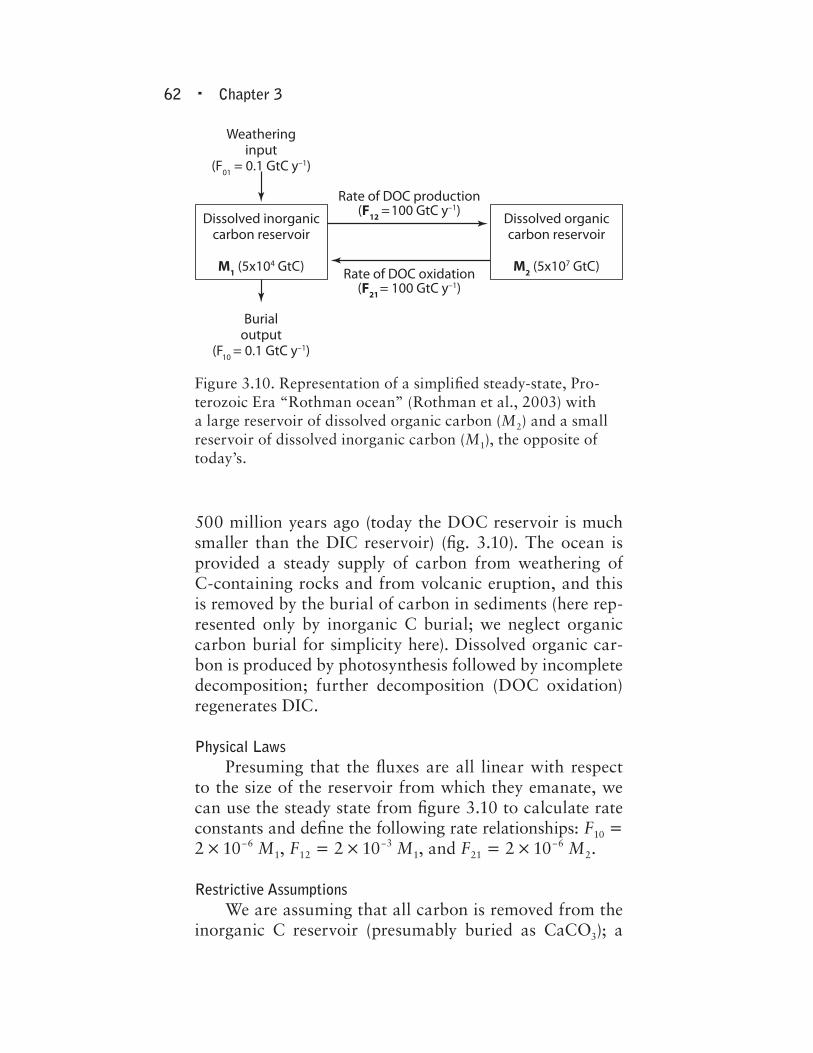
500 million years ago (today the DOC reservoir is much smaller than the DIC reservoir) (fig. 3.10). The ocean is provided a steady supply of carbon from weathering of C- containing rocks and from volcanic eruption, and this is removed by the burial of carbon in sediments (here rep-resented only by inorganic C burial; we neglect organic carbon burial for simplicity here). Dissolved organic car-bon is produced by photosynthesis followed by incomplete decomposition; further decomposition (DOC oxidation) regenerates DIC.
Physical LawsPresuming that the fluxes are all linear with respect
to the size of the reservoir from which they emanate, we can use the steady state from figure 3.10 to calculate rate constants and define the following rate relationships: F10 = 2 10−6 M1, F12 = 2 10−3 M1, and F21 = 2 10−6 M2.
Restrictive AssumptionsWe are assuming that all carbon is removed from the
inorganic C reservoir (presumably buried as CaCO3); a
Figure 3.10. Representation of a simplified steady- state, Pro-terozoic Era “Rothman ocean” (Rothman et al., 2003) with a large reservoir of dissolved organic carbon (M2) and a small reservoir of dissolved inorganic carbon (M1), the opposite of today’s.
Rate of DOC production(F12 = 100 GtC y–1)
Rate of DOC oxidation(F21 = 100 GtC y–1)
Weatheringinput
(F01 = 0.1 GtC y–1)
Burialoutput
(F10 = 0.1 GtC y–1)
Dissolved organiccarbon reservoir
M2 (5x10⁷ GtC)
Dissolved inorganiccarbon reservoir
M1 (5x10⁴ GtC)

Box Modeling • 63
more complete treatment would also consider the burial of organic matter. We are also neglecting the multitude of factors other than reservoir size that control these fluxes.
Perform the BalanceThe time rate of change of carbon in the DIC and
DOC reservoirs is the mass rate in minus the mass rate out; that is,
0.1 2 10 2 10
2 10dt
dMM M
M
1 62
61
31
# #
#
= + −
−
− −
− (3.40)
and
.dt
dMM M2 10 2 10 62 3
1 2# #= −− − (3.41)
Check UnitsAll terms in the equation above are expressed in units
of GtC y−1.
Define Interval, Specify Initial and Boundary ConditionsWe can solve for the steady state of the system by set-
ting equation 3.40 and equation 3.41 to zero, giving us two equations and two unknowns. The resulting steady states are
5 10M GtCss1
4#=
5 10 .M GtCss2
7#=
The DOC reservoir is 1,000 times larger than the DIC reservoir at steady state. Of course, we already knew the steady- state values because we used them to calculate the rate constants.
Let us presume we are interested in the response of the oceanic carbon cycle to a doubling of the riverine input F10 (from 0.1 to 0.2 GtC y−1). We use the forward Euler method with a time step (Dt) of 100 years (fig. 3.11).
In 10,000 years, reservoir 1 (the DIC reservoir) has adjusted to a new, apparent steady state, whereas the large

64 • Chapter 3
DOC reservoir (reservoir 2) is increasing. We know that the new steady- state sizes of M1 and M2 are going to be twice the initial sizes. The doubling of M2 will take some several hundred million years, though, so we need to per-form a longer simulation. However, to reduce the number of computations, we increase the step size (Dt) to 1,000 years and compare this result for the first 10,000 with that shown in figure 3.11. The result is shown in figure 3.12.
No, we haven’t discovered a natural behavior worthy of further investigation. We simply revealed numerical instability. This behavior is referred to as “sawtoothing” for obvious reasons. The solution has become unstable, oscillating about the exact solution, with the estimate of the derivative changing signs back and forth introducing large inaccuracies. The source of this problem is more eas-ily seen in the simple case of exponential decay, where the Euler solutions scheme is
(1 ) .y y tn n1 λD= −+ (3.42)
Figure 3.11. Solution to the Rothman ocean perturbation ( doubling of river C input) over the first 10,000 years. Note that the DIC reservoir (M1) has reached quasi- steady- state. Forward Euler method, 100- year time step.
Time (y)
50,06050,001,000
50,03050,000,500
50,00050,000,000
0 2,500 5,000 7,500
M1M2
10,000
Gto
ns C

Box Modeling • 65
Note here that if Dt > 2/ , the estimate of y changes sign every time step. Increasing the time step even further leads to even more erratic behavior with huge errors. If we wish to use this method, then, we are forced to use small, century- long time increments. But we want to integrate over 100 million years, thereby requiring a million time steps. Is there a more efficient way to perform this calcu-lation that allows larger time steps without jeopardizing stability?
Backward Euler Method
What if we could evaluate the derivative of the function at a future time step? Would knowing that derivative and using it to extrapolate forward in time improve the stabil-ity of the solution? To do so, we rewrite equation 3.28 as
.y ydtdy tn n1
n 1D= ++
+y (3.43)
For the problem of exponential decay (equation 3.34), this becomes
Time (y)
50,15050,002,000
50,05050,001,000
49,95050,000,000
0 2,500 5,000 7,500
M1M2
10,000
Gto
ns C
Figure 3.12. Same as figure 3.11, except now a step size of 1,000 years was specified, revealing “sawtoothing” behavior.

66 • Chapter 3
( ).
y y y t
ty
1
n n n
n
1 1λ
λ
D
D
= −
=+
+ +
(3.44)
Comparing equation 3.44 with equation 3.45, we note that now there is no apparent instability, and as Dt " ∞, the approximation converges on the true solution. Thus this method, known as the backward Euler method, is stable and gives accurate solutions at long times (although not on short times, but that is okay because we don’t care about the short timescales in this problem).
Of course, we don’t know the value of the derivative in the future a priori; equation 3.43, and the backward Euler method it represents, are implicit. However, we can approximate it using Taylor series,
,dtdy
dtdy
y dtdy y
1n n n22
. D++y y y
d n (3.45)
ignoring the higher- order terms in the series, and where Dy = yn+1 yn. Substituting equation 3.45 into equation 3.43 yields
.ydtdy
y dtdy y t
n n22
D D D= +y y
d n> H (3.46)
Now, gather terms to solve for Dy, because Dy gives us the increment in y that we need to calculate yn+1. After rearranging,
,yt y dt
dydtdy1
n n22
DD
− =y y
f d pnor
y
t y dtdy
dtdy
1n
n
22
D
D
=−
y
y
d n (3.47)
This is the backward Euler method for a single ODE. We can generalize this for a system of equations by defining the Jacobian matrix J as

Box Modeling • 67
( )Jy
F yn
22/
l v
and recognizing that I is the identity matrix:
( ) .JIt
y F y1 n
DD− = lv vd n (3.48)
Note that equation 3.48 is similar to the matrix form of the forward Euler method, except for the presence of the Jacobian matrix. Thus, we can imagine intermediate so-lution schemes between the forward and backward Euler methods and implement these in our codes by incorporat-ing a parameter q:
( ) .JIt
y F y1 nθD
D− = lv vd n (3.49)
When q = 0, we have the forward Euler method; when q = 1, we have the backward Euler method; and when q = 0.5, we have the Crank–Nicolson method. Crank– Nicolson blends the two methods and in doing so achieves a higher- order accuracy than either method without seri-ously compromising the stability attributes of the back-ward Euler method.
Returning to the Rothman ocean example, the F vec-tor is
0.1 2 10 2 10 2 102 10 2 10 ,F
M M MM M
62
61
31
31
61
# # #
# #=
+ − −−
− − −
− −l > H (3.50)
and the Jacobian matrix is
,J 2 10 2 102 10
2 102 10
6 3
3
6
6# #
###
= − −−
− −
−
−
−< F (3.51)
so equation 3.49 becomes:
..
It
y
M M MM M
1 2 10 2 102 10
2 102 10
0 1 2 10 2 10 2 102 10 2 10
6 3
3
6
6
62
61
31
31
61
# ##
##
# # #
# #
θD
D− − −−
=+ − −
−
− −
−
−
−
− − −
− −
vd n<>
FH
(3.52)

68 • Chapter 3
This algebraic equation is readily solved using MATLAB or any other linear algebra software that can do matrix inversion. Figure 3.13 compares the short- term (from a ge-ologist’s perspective, over 10,000 years) response of the DIC reservoir of the Rothman ocean to a doubling of the riverine input, computed with the forward Euler method (100- year time step) and the backward Euler method (1,000- year time step). Recall that the forward Euler ap-proach exhibited sawtoothing with a time step of 1,000 years (fig. 3.12). The backward Euler method does not sawtooth, but it consistently underestimates the true solu-tion (closely reflected in the forward Euler solution) over the first several thousand years.
However, by the time the DIC reservoir has reached quasi- steady- state (i.e., a slowly evolving steady state), the two solutions have converged. The great advantage of the implicit method (backward Euler) is shown in figure
50,060
50,030
50,040
50,050
50,020
50,010
50,0000 2,500 5,000 7,500
∆t = 100 y∆t = 1,000 y
10,000
Gto
ns C
Time (y)
Figure 3.13. Comparison between the forward and backward Euler solutions to the Rothman ocean perturbation over the first 10,000 years, with 100- year and 1,000- year time steps, respectively, for reservoir 1 (the DIC reservoir). Compare with figure 3.11.

Box Modeling • 69
3.14, which displays the evolution of the DIC and DOC reservoirs over 2 billion years. This same result is ob-tained with a time step of 1 million years, reflecting the method’s stability and convergence on the true solution on long times.
Model Enhancements
A computer code that incorporates the forward and back-ward Euler methods is quite flexible and can solve most problems of interest in box modeling. The methods as pre-sented do have some limitations, though. For example, the step size must be specified, and the Jacobian matrix must be obtained analytically. Of course, these problems can be overcome.
x 109
100
70
80
90
60
500 0.4 0.8 1.2 1.6 2
Figure 3.14. Evolution of the Rothman ocean DIC (×103 GtC) and DOC (×106 GtC) in response to a doubling of the riverine C input, calculated using a time step of 100,000 years and the backwards Euler method. The solution is essentially identical with a time step of 1 million years.

70 • Chapter 3
Automatic Step- Size AdjustmentFor stiff problems, in particular, it may be advisable
to adjust the time step as the simulation proceeds, keeping it short at first and then longer as the fast- response reser-voirs come to quasi- steady- state. Incorporating automatic step- size adjustment is quite simple. One simply assesses the change in reservoir size from one time step to the next relative to the initial reservoir size (j):
.y
y yn
n n1
ϕ =−+
(3.53)
If j is less than a tolerance limit (e, often set at 0.001), the step size is increased by an amplification factor, and the next time step is computed. If j is greater than e, the step size is diminished by a reduction factor and the time- step recomputed. One can also specify a maximum and mini-mum value of Dt to prevent round- off and truncation error accumulation. The logic here is that we are trying to keep the change in the solution from one time step to the next small relative to the magnitude of the solution to avoid large errors in the numerical approximation. There are no particular values of the amplification and retardation fac-tors that work for every application, but 0.5 and 2 (halving and doubling) are commonly used.
Numerical Approximation to the Jacobian Matrix (After Walker, 1991)
Finally, it is sometimes advantageous to make a nu-merical approximation to the Jacobian matrix when the ordinary differential equations are complex and nonlinear (i.e., when it is difficult or impossible to find the partial derivatives). To do so, first calculate the derivative vector F for the current values of yn
1v . Then increment yn
1v by a
small amount, typically a small multiplier of yn1v (e.g., yn
1ev , where e is typically 0.001), and recalculate the derivatives. Divide these numbers by e yi
n , change their sign, and to the diagonal term add 1/Dt. This gives you the first column in the Jacobian. Restore the value of yn
1v and then repeat
the procedure for yn2v , and so forth, to fill the Jacobian.

Box Modeling • 71
Summary
In this chapter, we explored the translation of simple geologic problems of conservation of mass or energy into systems of ordinary differential equations (i.e., box models). Such models are often called “toy” models, be-cause they are based on significant simplifications of the natural world. However, because they are based on the conservation equations, the results they produce are con-sistent with these laws, more than can often be said for the “arm waving” conclusions one might make in inter-preting data. Thus, they have real value for the geosci-entist interested in the big picture and/or in advance of more sophisticated modeling. One shortcoming of box modeling is that it generally specifies, rather than calcu-lates, the physics of flows. For that we turn to spatially dependent systems of equations, partial differential equa-tions, and their solutions: the topics of the remainder of this book.
Modeling Exercises
1. Runge–Kutta Scheme Write a simple code to solve the problem of radio active
decay numerically using a second- order Runge–Kutta solver (e.g., equation 3.38). Graph the analytic and numerical solutions using the initial condition and decay constant that generated table 3.1. Extra Credit: Find and code a fourth- order Runge–Kutta scheme, and compare its accuracy with that of the second- order scheme here.
2. The Oceanic Phosphate (P) Cycle a. Construct a simple box model (single ODE) of
the P cycle. Follow the proper steps of model building. Use the following information:
• Average concentration of P in ocean [PO4] = 2.1 10–6 mol kg–1 seawater.
• Mass of the ocean = 14 1020 kg.

72 • Chapter 3
• Average residence time of P in ocean (with respect to river input or sediment output) = 40,000 years.
• Assume that the sediment output is propor-tional to the average concentration.
b. Human activity has approximately doubled the input of phosphate to the ocean. Plot the re-sponse of the ocean’s P content to a doubling of the rate of riverine input. Be sure to carry the calculation out far enough to show the new steady state.
c. Now create a more sophisticated two- box model of the ocean’s P cycle. Divide the ocean into a surface box and a deep box. The surface box will have 2.5% of the mass of the deep box and a steady- state concentration 10% of the deep box. The total phosphate content of the ocean (i.e., the average concentration of phosphate) will be identical to that of part 1a, as will the total mass of the ocean. River input will be to the surface box. Use the following additional information to complete the model:
• The removal of phosphate from the surface box with biological productivity is propor-tional to the concentration of phosphate in that box.
• Ninety- nine percent of this flux is released to the deep ocean during decomposition, and 1% is removed to the sediments (balancing the river input at steady state).
• Water is mixed (upwelled and downwelled) between the surface and deep boxes at a rate of 14 1017 kg y–1, creating a net transfer of phosphate from deep to surface that is propor-tional to this rate, and the concentration dif-ference between deep and surface—that is, the rate (mol y–1) of phosphate added to the surface box—is (14 1017 kg y–1) ([PO4]d [PO4]s).
d. Finally, plot the response of the ocean’s phos-phate concentration (surface and deep) to a

Box Modeling • 73
doubling of the mixing rate between surface and deep. Be sure to carry the calculation out far enough to show the new steady state.
3. Stiff Systems and Implicit Solvers Use the forward and backward Euler scheme to
integrate the following set of ODEs (attributed to C. W. Gear) for 0 ≤ t ≤ 1 for an initial condition of y1(0) = 1, y2(0) = 0, and for time steps (Dt) of 0.001, 0.0018, 0.002, and 0.1, and compare the re-sults with the analytic solutions:
dtdy
y y998 199811 2= +
.dtdy
y y998 19991 22 = − −
The analytical solutions are
2y e e ,t t1
1 000= −− −
.y e e ,t t2
1 000= − +− −